ACTIVE VIBRATION CONTROL OF COMPLEX STRUCTURES IN

MODAL SPACE

A THESIS SUBMITTED TO

THE GRADUATE SCHOOL OF NATURAL AND APPLIED SCIENCES

OF

MIDDLE EAST TECHNICAL UNIVERSITY

BY

KEMAL MERSİN

IN PARTIAL FULFILLMENT OF THE

REQUIREMENTS

FOR

THE DEGREE OF MASTER OF SCIENCE

IN

MECHANICAL ENGINEERING

DECEMBER 2014

Approval of the thesis:

ACTIVE VIBRATION CONTROL OF COMPLEX STRUCTURES IN

MODAL SPACE

submitted by KEMAL MERSİN in partial fulfillment of the requirements for

the degree of Master of Science in Mechanical Engineering Department,

Middle East Technical University by,

Prof. Dr. Gülbin Dural Ünver

Dean, Graduate School of Natural and Applied Sciences

Prof. Dr. R. Tuna Balkan

Head of Department, Mechanical Engineering

Assist. Prof. Dr. Yiğit Yazıcıoğlu

Supervisor, Mechanical Engineering Dept., METU

Assoc. Prof. Dr. Melin Şahin

Co-Supervisor, Aerospace Engineering Dept., METU

Examining Committee Members:

Prof. Dr. Mehmet Çalışkan

Mechanical Engineering Dept., METU

Assist. Prof. Dr. Yiğit Yazıcıoğlu

Mechanical Engineering Dept., METU

Assoc. Prof. Dr. Melik Dölen

Mechanical Engineering Dept., METU

Assoc. Prof. Dr. Ender Ciğeroğlu

Mechanical Engineering Dept., METU

Assist. Prof. Dr. A. Türker Kutay

Aerospace Engineering Dept., METU

Date: 03.12.2014

iv

I hereby declare that all information in this document has been obtained

and presented in accordance with academic rules and ethical conduct. I also

declare that, as required by these rules and conduct, I have full cited and

referenced all material and results that are not original to this work.

Name, Last Name: Kemal Mersin

Signature:

v

ABSTRACT

ACTIVE VIBRATION CONTROL OF COMPLEX STRUCTURES IN

MODAL SPACE

Mersin, Kemal

M.S., Department of Mechanical Engineering

Supervisor: Assist. Prof. Dr. Yiğit Yazıcıoğlu

Co-Supervisor: Assoc. Prof. Dr. Melin Şahin

December 2014, 89 pages

Aerospace structures are designed to be light-weight to obtain high performance.

Reduction in weight makes the structure flexible and lower frequency modes can

be easily excited. Moreover those modes have low damping and vibrations do

not attenuate immediately. Passive systems are effective to control the vibrations

but they can be heavy and most of the time they do not respond to changing

environment conditions. An active system is necessary for low-weight adaptive

vibration reduction system.

Modal Space Control is used for large flexible aerospace structures due to the

advantage of reducing the complexity of control system. In this study a

generalized formulation of modal space control is proposed for three dimensions

where each node is modeled with six degrees of freedom.

Keywords: Active vibration control, state space control, modal control, finite

element analysis.

vi

ÖZ

MODAL UZAYDA KARMAŞIK YAPILARIN AKTİF TİTREŞİM

KONTROLÜ

Mersin, Kemal

Yüksek Lisans, Makina Mühendisliği Bölümü

Tez Yöneticisi: Yrd.Doç.Dr. Yiğit Yazıcıoğlu

Ortak Tez Yöneticisi: Doç.Dr. Melin Şahin

Aralık 2014, 89 sayfa

Yüksek performans elde etmek için havacılık ve uzay yapıları hafif olarak

tasarlanmaktadır. Ağırlığın azaltılması yapıyı daha esnek hale getirmekte ve

düşük frekanstaki modlar kolaylıkla tahrik edilebilmektedirler. Ayrıca bu

modlardaki sönümleme oranı düşüktür ve titreşimler hemen kaybolmamaktadır.

Pasif sistemler titreşimin sönümlenmesinde etkili olsalarda, ağır olabilirler ve

değişen çevre şartlarına çoğu zaman uyum sağlayamazlar. Hafif ve çevre

şartlarına uyum sağlayabilen titreşim azaltma sistemi için aktif titreşim kontrolü

gereklidir.

Kontrol sisteminin karmaşıklığını azaltması sebebiyle büyük ve esnek havacılık

ve uzay yapılarında Modal Uzay Kontrolü kullanılmaktadır. Bu çalışmada her

noktanın altı serbestlik derecesi ile modellendiği üç boyutlu yapılar için modal

uzay kontrolünün genel formülasyon önerilmiştir.

Anahtar Kelimeler: Aktif titreşim kontrolü, durum uzay kontrolü, modal control,

sonlu elemanlar analizi.

vii

To My Family

viii

ACKNOWLEDGMENTS

I would like to express my deep gratitude to my thesis supervisor Dr. Yiğit

Yazıcıoğlu for his motivation, encouragement and guidance during my thesis

work.

I am particularly grateful to my thesis co-supervisor Dr. Melin Şahin for his

support and advices on my theses.

I would like to thank to Dr. Buğra Koku for enlightening my way in

undergraduate courses and encouraging me through the graduate studies.

I would like to express my sincere appreciation to TAI and colleagues for

supporting me on vibration control studies topic.

Finally I would like to thank to my mother, father, sister, grandfather and

grandmother for their support, patience and assistance in this long period.

ix

TABLE OF CONTENTS

ABSTRACT ....................................................................................................... v

ÖZ ...................................................................................................................... vi

ACKNOWLEDGMENTS ............................................................................ viii

TABLE OF CONTENTS ................................................................................. ix

LIST OF TABLES ........................................................................................... xi

LIST OF FIGURES ....................................................................................... xii

ABBREVIATIONS ........................................................................................ xiv

CHAPTERS

1.INTRODUCTION .......................................................................................... 1

1.1 General Introduction ............................................................................. 1

1.2 Literature Review ................................................................................. 3

1.3 Problem Definition ............................................................................... 9

1.4 Motivation ............................................................................................ 9

1.5 Objective and Scope of This Thesis ..................................................... 9

2.MODAL SPACE REPRESENTATION OF A 1D STRUCTURE .......... 11

2.1 Introduction ........................................................................................ 11

2.2 Simply supported beam natural frequency and mode shapes ............. 11

2.3 Orthogonality of Modes and Expansion Theorem ............................. 14

2.4 Modal Domain Representation ........................................................... 17

2.5 Response to External Excitation ......................................................... 18

2.6 Systems with Proportional Modal Damping ...................................... 19

2.7 Transient and steady state response .................................................... 19

2.8 State Space Representation of a 1D Structure with Point Force ........ 20

2.9 Numerical Example ............................................................................ 23

2.9.1 Problem Definition ............................................................................... 23

2.9.2 Results .................................................................................................. 24

2.10 Numerical Example II ..................................................................... 25

3.DISCRETIZATION AND GENERALIZATION OF STATE SPACE

MODEL ............................................................................................................ 27

3.1 Introduction ........................................................................................ 27

3.2 Discretizing the 1D State Space Model .............................................. 27

3.3 Generalized State Space Approach in 3D .......................................... 28

3.4 Reducing the size of B, C, D Matrices ............................................... 31

x

3.5 Discrete Simply Supported Beam Compared With the Continuous

Model 32

3.6 Numerical Example for Complex Structure ....................................... 37

3.7 Comparison of FEA and State Space Model for Complex Structure. 42

4.MODAL SPACE CONTROL IN STATE SPACE ................................... 47

4.1 Introduction ........................................................................................ 47

4.2 Controller Design ............................................................................... 48

4.2.1 Pole Placement ..................................................................................... 48

4.2.2 Optimal Control .................................................................................... 50

4.2.3 Controllability ....................................................................................... 52

4.3 Observer Design ................................................................................. 53

4.3.1 Introduction ......................................................................................... 53

4.3.2 Observability ........................................................................................ 53

4.3.3 Observer Design ................................................................................... 54

4.4 Controlling Selected Modes ............................................................... 55

5.CASE STUDIES ........................................................................................... 57

5.1 Introduction ........................................................................................ 57

5.2 Simply Supported Beam .................................................................... 57

5.2.1 Model Definition .................................................................................. 57

5.2.2 Case Studies ......................................................................................... 59

5.3 Complex Structure ............................................................................. 65

5.3.1 Model Definition .................................................................................. 65

5.3.2 Case Studies ......................................................................................... 67

6.CONCLUSION ............................................................................................ 81

6.1 Discussion .......................................................................................... 81

6.2 Conclusion.......................................................................................... 82

6.3 Future Work ....................................................................................... 83

REFERENCES ................................................................................................ 85

APPENDICES

A.MATLAB CODE FOR FAST FOURIER TRANSFORM ....................... 89

xi

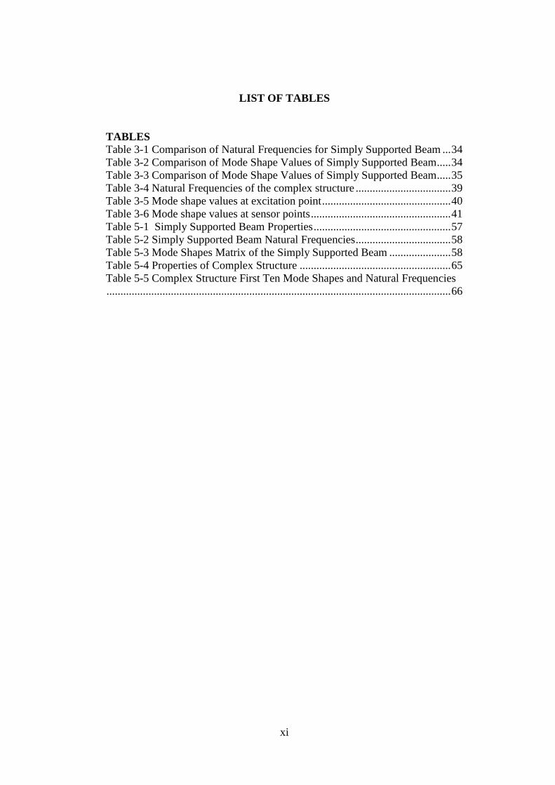
LIST OF TABLES

TABLES

Table 3-1 Comparison of Natural Frequencies for Simply Supported Beam ... 34 Table 3-2 Comparison of Mode Shape Values of Simply Supported Beam..... 34 Table 3-3 Comparison of Mode Shape Values of Simply Supported Beam..... 35 Table 3-4 Natural Frequencies of the complex structure .................................. 39 Table 3-5 Mode shape values at excitation point .............................................. 40

Table 3-6 Mode shape values at sensor points .................................................. 41 Table 5-1 Simply Supported Beam Properties ................................................. 57 Table 5-2 Simply Supported Beam Natural Frequencies .................................. 58 Table 5-3 Mode Shapes Matrix of the Simply Supported Beam ...................... 58

Table 5-4 Properties of Complex Structure ...................................................... 65 Table 5-5 Complex Structure First Ten Mode Shapes and Natural Frequencies

........................................................................................................................... 66

xii

LIST OF FIGURES

FIGURES

Figure 1-1 – Helicopter AVC Trend [1] ............................................................. 2 Figure 1-2 – International Space Station ............................................................ 3 Figure 1-3 Spaceraft Model ................................................................................ 6 Figure 1-4 Rotor Model ...................................................................................... 7 Figure 1-5 Experimental mode shapes, natural frequencies and damping ratio

of curved panels of car, ....................................................................................... 8 Figure 1-6 Adjusted Mode Shapes ...................................................................... 8 Figure 2-1 Euler Bernoulli Beam ...................................................................... 12 Figure 2-2 First three modes of simply supported beam .................................. 14

Figure 2-3 - Simulink Model of Open Loop State Space System .................... 24 Figure 2-4 Simply Supported Beam Response to 10 Hz Excitation ................. 24 Figure 2-5 Simply Supported Beam Response to 50 Hz Excitation ................. 25

Figure 2-6 Simply Supported Beam Intermediate Load Static Deflection ....... 25 Figure 2-7 Simply Supported Beam Response to Step Input and Steady State

Result ................................................................................................................ 26 Figure 3-1 Simply Supported Beam Model and Node Numbers ...................... 33

Figure 3-2 First Mode Shape ............................................................................ 33 Figure 3-3 Second Mode Shape ........................................................................ 33 Figure 3-4 Third Mode Shape ........................................................................... 33

Figure 3-5 Simply Supported Beam Response to 10 Hz sinusoidal excitation 36 Figure 3-6 Simply Supported Beam Response to 50 Hz sinusoidal excitation 36

Figure 3-7 Three dimensional complex structure with node numbers ............. 37 Figure 3-8 First three mode shapes of complex structure ................................. 38

Figure 3-9 Complex Structure Step Input from Y Axis ................................... 42 Figure 3-10 – Comparison of FEA and SS Responses to Step Input ............... 43

Figure 3-11 Error Percentage between FEA and SS Response to Step Input... 43 Figure 3-12 Complex Structure Sinusoidal Input from Y Axis ........................ 44 Figure 3-13 Comparison of SS and FEA Responses to Sinusoidal Disturbance

.......................................................................................................................... 44

Figure 3-14 Error Percentage between FEA and SS Response to Sinusoidal

Input .................................................................................................................. 45 Figure 4-1 Feedback Gain Controller in State Space ....................................... 47 Figure 4-2 Placement of Poles [35] .................................................................. 50 Figure 4-3 Uncontrollable and Controllable Systems [32] ............................... 53

Figure 4-4 Observer and Plant [38] .................................................................. 55 Figure 5-1 Node Numbers of Simply Supported Beam .................................... 58

Figure 5-2 Simply Supported Beam Response to Step Input ........................... 59 Figure 5-3 Simply Supported Beam Force Comparison to Step Response

Disturbance ....................................................................................................... 60 Figure 5-4 SSB Step Response Coupled Optimal Control for Different R values

(displacement) ................................................................................................... 61

Figure 5-5 SSB Step Response Coupled Optimal Control for Different R values

(Force) ............................................................................................................... 61

xiii

Figure 5-6 SSB Step Response Independent Optimal Control for Different R

values (displacement) ........................................................................................ 62 Figure 5-7 SSB Step Response Independent Optimal Control for Different R

values (displacement) ........................................................................................ 62

Figure 5-8 Simply Supported Beam, Frequency Response Function between 0-

100 Hz, One Mode Control ............................................................................... 63 Figure 5-9 Simply Supported Beam, Frequency Response Function between 0-

100 Hz, Two Mode Control, Sensor at 7th Node. .............................................. 64 Figure 5-10 Simply Supported Beam, Frequency Response Function between

0-100 Hz, Two Mode Control, Sensor at 14th Node. ........................................ 65 Figure 5-11 Complex Structure with Finite Element Node Numbers............... 66 Figure 5-12 Complex Structure response to Step Input. Sensor Z axis, Actuator

Z axis, Co-placed. ............................................................................................. 68

Figure 5-13 Complex Structure response to Step Input. Sensor Y axis, Actuator

Z axis, Co-placed .............................................................................................. 69 Figure 5-14 Complex Structure response to Step Input. Sensor Z axis, Actuator

Z axis, Not Co-placed ....................................................................................... 70 Figure 5-15 Complex Structure response to Step Input. Sensor Y axis, Actuator

Z axis, Not Co-placed ....................................................................................... 71 Figure 5-16 Complex Structure response to Chirp Signal from 2 Hz to 100 Hz.

Sensor Y axis, Actuator Z axis, Not Co-placed ................................................ 72 Figure 5-17 Complex Structure, response to step input X axis results. ............ 73 Figure 5-18 Complex Structure, response to step input Y axis results ............. 73

Figure 5-19 Complex Structure, response to step input X axis results. Non Co-

placed sensor and actuator ................................................................................ 74

Figure 5-20 Complex Structure, response to step input Y axis results. Non Co-

placed sensor and actuator ................................................................................ 75

Figure 5-21 Complex Structure, X axis sensor frequency response function.

Non Co-placed sensor and actuator................................................................... 76

Figure 5-22 Complex Structure, Y axis sensor frequency response function.

Non Co-placed sensor and actuator................................................................... 77 Figure 5-23 Local Mode Control Results to Step Input .................................... 78 Figure 5-24 Frequency Response Function of Local Mode Control to A Chirp

Excitation .......................................................................................................... 79 Figure 5-25 Frequency Response Function of Local Mode Control to A Chirp

Excitation Close Up View First and Second Mode .......................................... 79 Figure 5-26 Frequency Response Function of Local Mode Control to A Chirp

Excitation Close Up View Third Mode ............................................................ 80

Figure 5-27 Frequency Response Function of Local Mode Control to A Chirp

Excitation Close Up View Fifth Mode.............................................................. 80

xiv

ABBREVIATIONS

SDOF : Single Degree of Freedom

FEA : Finite Element Analysis

FEM : Finite Element Method

IMSC : Independent Modal Space Control

N : Number of nodes

m : Number of modes

mc : Number of controlled modes

mr : Number of residual modes

d : Number of degrees of freedom

DOF : Degrees of Freedom

η : Modal displacement

ϕ : Mode shape vector

Φ : Mode shape matrix

I : Identity matrix

Ω : Natural frequency in rad/sec

ζ : Modal damping ratio

1

CHAPTER 1

INTRODUCTION

1.1 General Introduction

Rigidity and weight are often competing objectives for high performance

structures such as the ones in aerospace applications. In these structures, first

natural frequencies and damping ratios at those frequencies are usually quite

low. Therefore, they are prone to high vibration levels during normal operation.

Excessive vibration may cause the following problems in these applications:

Disturbs the crew through vibration and noise

Decreases service life

Damages electronic components

Damages the structure

Reduces the accuracy of precise structures

Helicopter applications can be taken as an example for such high performance

structures where rotor is the main vibration source. N/rev frequency vibration in

the helicopter is dominant excitation. For the constant rotor speed helicopter’s

passive vibration isolation systems are effective in forward flight / hover

conditions. Those systems are heavy and ineffective at maneuvering flight and

requires continuous maintenance. Their performance degrade due to the

changing properties of system. Furthermore they are not adaptive for rotor

rotation speed changes. Active systems can overcome the weight problem, and

they can adapt to changing conditions. [1, 2]. The current trend in helicopter

vibration control is given in Figure 1-1 where weight reduction with increased

efficiency is required.

2

Figure 1-1 – Helicopter AVC Trend [1]

Satellites are another type of high performance lightweight and underdamped

structures that can be excited due to the maneuvers in space. Solar panels and

antennas can oscillate for extended periods with those excitations. This type of

vibrations reduce the accuracy of the sensors such as telescopes or synthetic

aperture radars. [3, 4, 5], Vibrations also degrade the performance of cameras on

board [6]. An image of international space station is presented in Figure 1-2 to

show the solar panels. Each panel length is 33 meters and width is 4.6 meters.

Their first two modes are 0.6 and 0.8 Hz. In addition to operational vibrations in

space, satellites are affected by high vibrations during launch due to the

combustion instability [7, 8] which produce longitudinal vibrations. For example

Apollo 13 was subject to 34g vibration level at 16 Hz.

3

Figure 1-2 – International Space Station

1.2 Literature Review

Controlling vibrations of large flexible structures in physical domain is a high

degree of freedom problem. Meirovitch and Balas proposed a new control

algorithm called modal space control, where vibrations are controlled in modal

domain [9, 10]. Therefore degrees of freedom of the system model reduce to the

number of modelled modes.

Optimal control strategies such as Linear Quadratic Regulator (LQR) and Linear

Quadratic Gaussian (LQG) has been studied for modal space control. . Optimal

control is also applied to damped gyroscopic systems [11, 12, 13].

Modal space control is first designed for distributed systems. It is expanded to

discrete systems for point acted sensors and actuators. Modal filters and

interpolation functions are used for this expansion [14].

In the distributed system, considering infinity modes, there are no observer or

control spillover problems. However in reality it is necessary to truncate

modelled modes where observation spillover can be a problem. By increasing

number of modelled modes, observation spillover can be solved [15].

4

Active vibration control is used to control low frequency vibrations. The effects

of controller to higher modes create control spillover problem. However exciting

higher modes requires more energy, those modes have lower amplitudes and due

their random nature they cancel each other [14].

It is observed in the literature that optimal placement of sensors and actuators

for modal space control is studied for plate type structures [16, 17, 18].

Integrated structural design with active vibration control has also been

investigated with modal space control to optimize actuator and sensor locations

while minimizing the mass of the structure [19, 20].

Modal space control is divided into two sub divisions called coupled control and

Independent Modal Space Control (IMSC). In IMSC each mode is controlled

separately and every modal equation is decoupled. Designing control systems

for IMSC is easy and finding global minimum is possible. In coupled control

less number of actuators can be used however the performance is sensitive to

actuator locations and finding global minimum is not always possible [21].

Meirovitch and Baruh shown that independent modal space control close loop

system is guaranteed to be stable. It is stated that any error in mass or stiffness

matrices does not create any instabilities in the closed loop system where an

appropriate feedback matrix is chosen [22].

In normal IMSC approach, a separate actuator is required for controlling each

mode. In [16] a new formulation is proposed to optimal control law to control

same number of modes with less actuators. In spite of this advantages, now the

quadratic cost function does not reflect one-to-one correspondence between

adjustable parameters and actuators control effort and the connection between

state penalty and state performance is indirect. Therefore, tuning of the controller

is more troublesome. The third problem is that in this approach stability is not

assured and one must take care of stability during the adjustment of controller

parameters.

5

Baz, Poh and Studer suggested a modified independent modal space control

(MIMSC) method to overcome spillover problem in IMSC [23]. They also

offered an optimal actuator placement technique, uni-variate search method

which varies the location of one actuator at a time in order to minimize a cost

function. It is stated that optimal controller solves the problem in modal domain,

an optimal location is necessary to minimize control forces in actual domain.

Thirdly, a time sharing methodology is studied where small number of actuators

suppress large number of modes. Two strategies are suggested, first is sequential

which every mode is given a fixed amount of time to suppress vibrations. Second

method is based on modal energy where the highest energy n number of modes

are suppressed with n number of actuators. The drawback of time sharing is

actuators are required to have wide bandwidth.

Singh proposes an efficient modal control algorithm which improves the

MIMSC algorithm. In MIMSC when energy in each mode is equal, controller

chatters. With the proposed algorithm the chatter is prevented where each mode

weight is proportional to its displacement or energy content. Also in this paper

it is shown that one piezo-electric actuator can be used to control more than one

mode [24].

In Öz’s paper it is stated that the main criticism of IMSC is that it requires many

actuators and sensors to be implemented in real structures [25]. Öz has made the

connection between the piezoelectric patches with independent modal space

control approach in his paper. It is shown that one piezoelectric patch can be

used to reduce vibrations of more than one mode [24].

Fang et al. proposed a modified independent modal space control algorithm to

solve spillover problem for uncontrolled modes [26]. They have suggested a new

feedback algorithm where uncontrolled modeled modes spillover can be

prevented as long as controller design follows the given rules in the paper. The

effects of residual modes and their connection with optimal controller law is

shown mathematically and nullifying them solves the spillover problem.

6

Silva and Inman has studied IMSC on internal variable based viscoelastic bar

considering the internal variables [23]. A finite element model for longitudinal

vibrations of viscoelastic elements are built. The model is one-dimensional with

one degrees of freedom. IMSC is tested numerically and the reduction of

vibration is satisfactory. It is stated that viscoelastic material have high damping

at higher frequencies and IMSC can be used for only suppressing lower modes

which makes IMSC an attractive approach to be used with viscoelastic systems.

Raja et al. studied the effects of one and two dimensional piezoelectric actuation

on smart panels where IMSC is used as the controller. Directional piezoelectric

and isotropic piezoelectric actuation behavior is compared numerically on

aluminum plates. Plates are modeled with four-node Mindlin-Reissner plate

element. The model is three dimensional containing five degrees of freedom.

Mode shapes are found with finite element analysis.

In a study by Meirovitch and Oz, a flexible spacecraft is considered with 12

modes of two cantilever appendages in three dimensions shown in Figure 1-3.

Assumed functions are used as mode shapes. Moreover rigid modes of the

spacecraft both translation and rotation were controlled with the actuators

located at the center [11].

Figure 1-3 Spaceraft Model

7

In [27] a non-classically damped gyroscopic system is studied by Lin and Yu.

Mode shapes are calculated by mode shape functions. The system is one

dimensional where degrees of freedom of each node is four with two translations

and two rotations. IMSC is effectively applied on the system.

Figure 1-4 Rotor Model

Houlstan et al. presented a novel modal control method that can be applied to

the non-classically damped systems. A similar model shown in Figure 1-4 is

numerically tested with the new control algorithm [28].

Hurlebaus et al studied IMSC on curved panels. In the study they have found

mode shapes with experimental modal analysis. They modeled the structure in

three dimensions x, y, z and used three degrees of freedom in each orthogonal

translation axis. An experimental modal control study is carried out and it is

shown that IMSC can be applied on curved panels. Mode shapes of the curved

panel is shown in Figure 1-5 [29].

8

Figure 1-5 Experimental mode shapes, natural frequencies and damping

ratio of curved panels of car,

Serra, Resta and Ripamonti proposed a new method called dependent modal

space controller where in addition to IMSC, mode shapes can be altered to create

nodes at wanted locations [30]. However to alter mode shapes more control force

is required. A cantilever beam with mode shapes taken from finite element

analysis is numerically tested. In Figure 1-6 the adjusted first three mode shapes

of the cantilever beam are shown.

Figure 1-6 Adjusted Mode Shapes

9

1.3 Problem Definition

Large flexible structures have low frequency and low damping in the first modes

which requires attention to prevent excessive vibration levels. Passive solutions

are too heavy to be implemented on to aerospace structures. Therefore an active

vibration control solution is required.

1.4 Motivation

Controlling the first modes of large flexible structures is necessary due to the

points stated in the problem definition. An implementation on complex shapes

is not frequently encountered in literature. In this study, implementation of

modal space control approach will be extended to an arbitrary 3-D complex

shape.

1.5 Objective and Scope of This Thesis

The objective of this study is to propose a generalized formulation in three

dimensions and show that modal space control can be applied to complex

structures. The outline of the thesis is as follows; a general introduction and

literature survey is presented in Chapter 1. Modal space representation of a one

dimensional structure is given in the Chapter 2. Discretization and generalization

of a three dimensional structure in modal space is studied in Chapter 3. In

Chapter 4 controller and observer design is shown. Case studies for simply

supported beam and a three dimensional shape is presented in Chapter 5.

Discussion, conclusion and future work is given in the Chapter 6.

10

11

CHAPTER 2

MODAL SPACE REPRESENTATION OF A 1D STRUCTURE

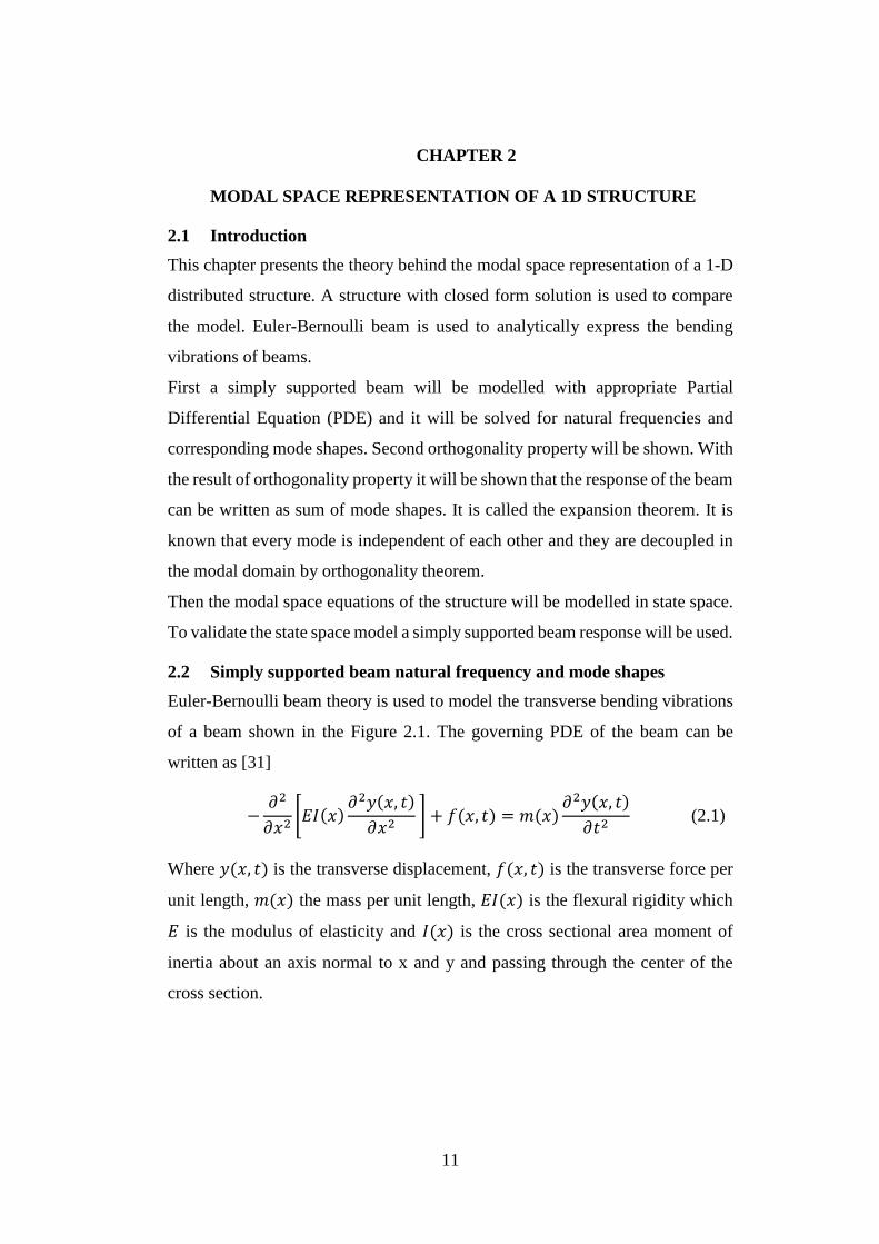
2.1 Introduction

This chapter presents the theory behind the modal space representation of a 1-D

distributed structure. A structure with closed form solution is used to compare

the model. Euler-Bernoulli beam is used to analytically express the bending

vibrations of beams.

First a simply supported beam will be modelled with appropriate Partial

Differential Equation (PDE) and it will be solved for natural frequencies and

corresponding mode shapes. Second orthogonality property will be shown. With

the result of orthogonality property it will be shown that the response of the beam

can be written as sum of mode shapes. It is called the expansion theorem. It is

known that every mode is independent of each other and they are decoupled in

the modal domain by orthogonality theorem.

Then the modal space equations of the structure will be modelled in state space.

To validate the state space model a simply supported beam response will be used.

2.2 Simply supported beam natural frequency and mode shapes

Euler-Bernoulli beam theory is used to model the transverse bending vibrations

of a beam shown in the Figure 2.1. The governing PDE of the beam can be

written as [31]

−𝜕2

𝜕𝑥2[𝐸𝐼(𝑥)

𝜕2𝑦(𝑥, 𝑡)

𝜕𝑥2 ] + 𝑓(𝑥, 𝑡) = 𝑚(𝑥)

𝜕2𝑦(𝑥, 𝑡)

𝜕𝑡2 (2.1)

Where 𝑦(𝑥, 𝑡) is the transverse displacement, 𝑓(𝑥, 𝑡) is the transverse force per

unit length, 𝑚(𝑥) the mass per unit length, 𝐸𝐼(𝑥) is the flexural rigidity which

𝐸 is the modulus of elasticity and 𝐼(𝑥) is the cross sectional area moment of

inertia about an axis normal to x and y and passing through the center of the

cross section.

12

Figure 2-1 Euler Bernoulli Beam

It is known that the spatial solution is independent from the temporal solution

which implies that the 𝑦 and 𝑡 are separable variables. Then the displacement

can be expressed as

𝑦(𝑥, 𝑡) = 𝑌(𝑥)𝐹(𝑡) (2.2)

Placing (2.2) into (2.1), neglecting the force term and dividing both sides by

F(t) , equation (2.1) reduces to

𝑑2

𝑑𝑥2[𝐸𝐼(𝑥)

𝑑2𝑌(𝑥)

𝑑𝑥2] = 𝜔2𝑚(𝑥)𝑌(𝑥), 0 < 𝑥 < (2.3)

Simply supported beam is pinned from two ends. The boundary conditions for

pinned end are zero displacement and zero moment at the pinned point. It can be

written as

𝑌(𝑥) = 0, 𝑀(𝑥, 𝑡) = 𝐸𝐼(𝑥)𝑑2𝑌(𝑥)

𝑑𝑥2= 0 (2.4)

For demonstration a beam with constant cross section area and material

properties with length 𝐿 will be used. No external force is given. Then the

equation (2.1) reduces to

𝑑4𝑌(𝑥)

𝑑𝑥4− 𝛽4𝑦 = 0, 0 < 𝑥 < 𝐿; , 𝛽4 =

𝜔2𝑚

𝐸𝐼 (2.5)

And boundary conditions are

13

𝑌(𝑥) = 0,𝑑2𝑌(𝑥)

𝑑𝑥2= 0, 𝑥 = 0, 𝐿 (2.6)

Assume a solution for equation (2.5) as

𝑌(𝑥) = 𝐴𝑠𝑖𝑛𝛽𝑥 + 𝐵𝑐𝑜𝑠𝛽𝑥 + 𝐶𝑠𝑖𝑛ℎ𝛽𝑥 + 𝐷𝑐𝑜𝑠ℎ𝛽𝑥 (2.7)

The 𝐴, 𝐵, 𝐶, 𝐷 constants will be evaluated from the boundary conditions. Only

three constants can be found and the fourth will be written to derive the

characteristic equation for 𝛽. From the boundary conditions,

𝑑2𝑌(𝑥)

𝑑𝑥2= 𝛽2[−𝐴𝑠𝑖𝑛𝛽𝑥 − 𝐵𝑐𝑜𝑠𝛽𝑥 + 𝐶𝑠𝑖𝑛ℎ𝛽𝑥 + 𝐷𝑐𝑜𝑠ℎ𝛽𝑥] (2.8)

At x = 0 it can be written that

𝑌(0) = 𝐵 + 𝐷 = 0 (2.9)

And

𝑑2𝑌(𝑥)

𝑑𝑥2𝑥=0

= −𝐵 + 𝐷 = 0 (2.10)

Which implies that 𝐵 = 𝐷 = 0. At 𝑥 = 𝐿 it can be written that

𝑌(𝐿) = 𝐴𝑠𝑖𝑛𝛽𝐿 + 𝐶𝑠𝑖𝑛ℎ𝛽𝐿 = 0 (2.11)

And

𝑑2𝑌(𝑥)

𝑑𝑥2𝑥=𝐿

= 𝛽2(−𝐴𝑠𝑖𝑛𝛽𝐿 + 𝐶𝑠𝑖𝑛ℎ𝛽𝐿) = 0 (2.12)

𝛽 = 0 is a trivial solution so it is not a solution. It implies that 𝐶 = 0 and

𝑠𝑖𝑛𝛽𝐿 = 0 (2.13)

(2.13) is the characteristic equation for simply supported beam. The solution of

this equation consists of infinite number of eigenvalues

𝐵𝑟𝐿 = 𝑟𝜋, 𝑟 = 1,2, … (2.14)

Then the eigenfunctions can be written by equating 𝐵, 𝐶, 𝐷 to 0 and re-writing

the equation (2.7) with (2.14);

14

𝑌𝑟(𝑥) = 𝐴𝑟𝑠𝑖𝑛𝛽𝑟𝑥 = 𝐴𝑟𝑠𝑖𝑛𝑟𝜋𝑥

𝐿 , 𝑟 = 1,2, … (2.15)

The natural frequencies of the system can be found from

𝛽4 =𝜔2𝑚

𝐸𝐼 (2.16)

Then using equation (2.14) and rewriting (2.16) will yield

𝜔𝑟 = 𝑟2𝜋2√𝐸𝐼

𝑚𝐿4 , 𝑟 = 1,2, … (2.17)

First three modes of simply supported beam are drawn below in Figure 2-2.

Figure 2-2 First three modes of simply supported beam

2.3 Orthogonality of Modes and Expansion Theorem

Consider two distinct solutions for equation (2.15) and (2.17) as

𝑌𝑟(𝑥), 𝜔𝑟2 𝑎𝑛𝑑 𝑌𝑠(𝑥),𝜔𝑠

2 and write the governing beam equation

15

𝑑2

𝑑𝑥2[𝐸𝐼(𝑥)

𝑑2𝑌𝑟(𝑥)

𝑑𝑥2] = 𝜔𝑟

2𝑚(𝑥)𝑌𝑟(𝑥) , 0 < 𝑥 < 𝐿 (2.18)

And

𝑑2

𝑑𝑥2[𝐸𝐼(𝑥)

𝑑2𝑌𝑠(𝑥)

𝑑𝑥2] = 𝜔𝑠

2𝑚(𝑥)𝑌𝑠(𝑥) , 0 < 𝑥 < 𝐿 (2.19)

Then multiply (2.18) with 𝑌𝑠(𝑥) and integrate over 𝐿. Then rewrite it,

∫𝑌𝑠(𝑥)𝑑2

𝑑𝑥2[𝐸𝐼(𝑥)

𝑑2𝑌𝑟(𝑥)

𝑑𝑥2] 𝑑𝑥

𝐿

0

= 𝜔𝑟2 ∫ 𝑚(𝑥)𝑌𝑠(𝑥)𝑌𝑟(𝑥)

𝐿

0

𝑑𝑥 (2.20)

Integrating by parts the left side twice we obtain the following equation

∫𝑌𝑠(𝑥)𝑑2

𝑑𝑥2[𝐸𝐼(𝑥)

𝑑2𝑌𝑟(𝑥)

𝑑𝑥2] 𝑑𝑥

𝐿

0

= 𝑌𝑠(𝑥)𝑑

𝑑𝑥[𝐸𝐼(𝑥)

𝑑2𝑌𝑟(𝑥)

𝑑𝑥2]𝐿 0

− [𝑑𝑌𝑠(𝑥)

𝑑𝑥𝐸𝐼(𝑥)

𝑑2𝑌𝑟(𝑥)

𝑑𝑥2]𝐿 0

+ ∫ 𝐸𝐼(𝑥)𝑑2𝑌𝑟(𝑥)

𝑑𝑥2

𝑑2𝑌𝑠(𝑥)

𝑑𝑥2

𝐿

0

(2.21)

For pinned case, the boundary conditions from (2.6) imply that

𝑑2𝑌(𝑥)

𝑑𝑥2= 0, 𝑥 = 0, 𝐿

Then (2.21) is reduced to

∫ 𝐸𝐼(𝑥)𝑑2𝑌𝑟(𝑥)

𝑑𝑥2

𝑑2𝑌𝑠(𝑥)

𝑑𝑥2

𝐿

0

(2.22)

Putting (2.22) into (2.18) gives

∫ 𝐸𝐼(𝑥)𝑑2𝑌𝑟(𝑥)

𝑑𝑥2

𝑑2𝑌𝑠(𝑥)

𝑑𝑥2

𝐿

0

= 𝜔𝑟2 ∫ 𝑚(𝑥)𝑌𝑠(𝑥)𝑌𝑟(𝑥)

𝐿

0

𝑑𝑥 (2.23)

Similarly multiplying 2.19 with 𝑌𝑟(𝑥) and integrating over 𝐿 with same

procedures (2.20) becomes

16

∫ 𝐸𝐼(𝑥)𝑑2𝑌𝑟(𝑥)

𝑑𝑥2

𝑑2𝑌𝑠(𝑥)

𝑑𝑥2

𝐿

0

= 𝜔𝑠2 ∫ 𝑚(𝑥)𝑌𝑠(𝑥)𝑌𝑟(𝑥)

𝐿

0

𝑑𝑥 (2.24)

Subtracting (2.24) from (2.23)

(𝑤𝑟2 − 𝑤𝑠

2)∫ 𝑚(𝑥)𝑌𝑠(𝑥)𝑌𝑟(𝑥)𝐿

0

𝑑𝑥 = 0 (2.25)

So for distinct solutions, 𝑤𝑟 ≠ 𝑤𝑠 then this states that

∫ 𝑚(𝑥)𝑌𝑠(𝑥)𝑌𝑟(𝑥)𝐿

0

𝑑𝑥 = 0, 𝑟 ≠ 𝑠 (2.26)

And from (2.18) it can be written that

∫𝑌𝑠(𝑥)𝑑2

𝑑𝑥2[𝐸𝐼(𝑥)

𝑑2𝑌𝑟(𝑥)

𝑑𝑥2] 𝑑𝑥

𝐿

0

= 0, 𝑟 ≠ 𝑠 (2.27)

When r=s, equation (2.26) and (2.27) are not zero, and 𝑌(𝑥) can be such that

(2.26) and (2.27) becomes

∫ 𝑚(𝑥)𝑌𝑟(𝑥)𝑌𝑟(𝑥)𝐿

0

𝑑𝑥 = 1, 𝑟 = 1,2, … (2.28)

∫𝑌𝑟(𝑥)𝑑2

𝑑𝑥2[𝐸𝐼(𝑥)

𝑑2𝑌𝑟(𝑥)

𝑑𝑥2] 𝑑𝑥

𝐿

0

= 𝜔𝑟2 , 𝑟 = 1,2, … (2.29)

Then it is possible to write from equations (2.28) and (2.29) the expansion

theorem as

“Any function Y(x) representing a possible displacement of the beam, which

implies that Y(x) satisfies boundary conditions of the problem and is such that

(d2/dx2)(EI(x)d2Y(x)/dx2] is continuous, can be expanded in the absolutely and

uniformly convergent series of the eigenfunctions

𝑌(𝑥) = ∑𝑐𝑟𝑌𝑟(𝑥)

∞

𝑟=1

(2.30)

Where the constant coefficients cr are defined by

17

𝑐𝑟 = ∫ 𝑚(𝑥)𝑌𝑠(𝑥)𝑌(𝑥)𝐿

0

𝑑𝑥, 𝑟 = 1,2, … (2.31)

And

𝜔𝑟2𝑐𝑟 = ∫𝑌𝑟(𝑥)

𝑑2

𝑑𝑥2[𝐸𝐼(𝑥)

𝑑2𝑌(𝑥)

𝑑𝑥2] 𝑑𝑥

𝐿

0

, 𝑟 = 1,2, … " (2.32)

This states that any arbitrary displacement of the beam can be written as a sum

of its eigenfunctions and its response to initial conditions or external forces can

be calculated.

2.4 Modal Domain Representation

The expansion theorem does not cover time response of the beam. For the beam

equation assume a solution for 𝑦(𝑥, 𝑡) in the following form

𝑦(𝑥, 𝑡) = ∑𝜙𝑟(𝑥)𝜂𝑟(𝑡)

∞

𝑟=1

(2.33)

Where 𝜙𝑟 is the mass normalized modes of the system and 𝜂𝑟(𝑡) are time

dependent functions. Then placing (2.33) into (2.1) yields

−∑

𝑑2

𝑑𝑥2[𝐸𝐼(𝑥)

𝑑2𝜙𝑟(𝑥)

𝑑𝑥2 ] 𝜂𝑟(𝑡) = ∑𝑚(𝑥)𝜙𝑟(𝑥)

𝑑2𝜂𝑟(𝑡)

𝑑𝑡2

∞

𝑟=1

,

∞

𝑟=1

0 < 𝑥 < 𝐿

(2.34)

Then multiply (2.34) by 𝜙𝑠 and integrate over 𝐿

−∑ ∫{𝜙𝑠(𝑥)𝑑2

𝑑𝑥2[𝐸𝐼(𝑥)

𝑑2𝜙𝑟(𝑥)

𝑑𝑥2 ] 𝑑𝑥}

𝐿

0

𝜂𝑟(𝑡)

∞

𝑟=1

= ∑[∫𝑚(𝑥)𝜙𝑠(𝑥)𝜙𝑟(𝑥)𝑑𝑥

𝐿

0

]𝑑2𝜂𝑟(𝑡)

𝑑𝑡2

∞

𝑟=1

(2.35)

From the orthonormality equations (2.26)-(2.29) we obtain the independent set

of modal equations.

�̈�𝑟(𝑡) + 𝜔𝑟2𝜂𝑟(𝑡) = 0, 𝑟 = 1,2… (2.36)

Here, r represents the modal coordinate index. And the transformation between

real coordinates and modal coordinates are defined with the equation (2.33).

18

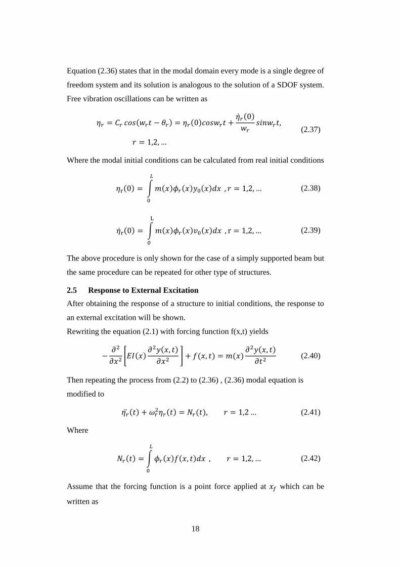
Equation (2.36) states that in the modal domain every mode is a single degree of

freedom system and its solution is analogous to the solution of a SDOF system.

Free vibration oscillations can be written as

𝜂𝑟 = 𝐶𝑟 𝑐𝑜𝑠(𝑤𝑟𝑡 − 𝜃𝑟) = 𝜂𝑟(0)𝑐𝑜𝑠𝑤𝑟𝑡 +

�̇�𝑟(0)

𝑤𝑟𝑠𝑖𝑛𝑤𝑟𝑡,

𝑟 = 1,2, …

(2.37)

Where the modal initial conditions can be calculated from real initial conditions

𝜂r(0) = ∫𝑚(𝑥)𝜙𝑟(𝑥)𝑦0(𝑥)𝑑𝑥

𝐿

0

, 𝑟 = 1,2, … (2.38)

�̇�r(0) = ∫𝑚(𝑥)𝜙𝑟(𝑥)𝑣0(𝑥)𝑑𝑥

L

0

, r = 1,2, … (2.39)

The above procedure is only shown for the case of a simply supported beam but

the same procedure can be repeated for other type of structures.

2.5 Response to External Excitation

After obtaining the response of a structure to initial conditions, the response to

an external excitation will be shown.

Rewriting the equation (2.1) with forcing function f(x,t) yields

−𝜕2

𝜕𝑥2[𝐸𝐼(𝑥)

𝜕2𝑦(𝑥, 𝑡)

𝜕𝑥2 ] + 𝑓(𝑥, 𝑡) = 𝑚(𝑥)

𝜕2𝑦(𝑥, 𝑡)

𝜕𝑡2 (2.40)

Then repeating the process from (2.2) to (2.36) , (2.36) modal equation is

modified to

𝜂�̈�(𝑡) + 𝜔𝑟2𝜂𝑟(𝑡) = 𝑁𝑟(𝑡), 𝑟 = 1,2… (2.41)

Where

𝑁𝑟(𝑡) = ∫𝜙𝑟(𝑥)𝑓(𝑥, 𝑡)𝑑𝑥

𝐿

0

, 𝑟 = 1,2, … (2.42)

Assume that the forcing function is a point force applied at 𝑥𝑓 which can be

written as

19

𝑓(𝑥, 𝑡) = 𝛿(𝑥 − 𝑥𝑓)𝐹(𝑡) (2.43)

Where

𝛿(𝑥 − 𝑥𝑓) = 1 𝑤ℎ𝑒𝑛 𝑥 = 𝑥𝑓 (2.44)

𝛿(𝑥 − 𝑥𝑓) = 0 𝑤ℎ𝑒𝑛 𝑥 ≠ 𝑥𝑓 (2.45)

Then the integration at (2.42) reduces to

𝑁𝑟(𝑡) = 𝜙𝑟(𝑥𝑓)𝐹(𝑡) (2.46)

And for point force modal equation can be written as

𝜂�̈�(𝑡) + 𝜔𝑟2𝜂𝑟(𝑡) = 𝜙𝑟(𝑥𝑓)𝐹(𝑡), 𝑟 = 1,2… (2.47)

This concludes the undamped equation for the state space representation of a

structure with a point force acting at point f.

2.6 Systems with Proportional Modal Damping

To complete the formulation, damping needs to be added to the model. Up to

this point, it is shown that a structure can be modelled as a sum of infinite number

of single degree of freedom systems in modal domain with modal mass and

modal stiffness.

For an SDOF system, a damping ratio of 𝜁𝑟 for the rth mode can be implemented

into the equation (2.47) analogous to SDOF vibratory systems as

𝜂�̈�(𝑡) + 2𝜔𝑟𝜁𝑟�̇�(𝑡) + 𝜔𝑟

2𝜂𝑟(𝑡) = 𝜙𝑟(𝑥𝑓)𝐹(𝑡),

𝑟 = 1,2…

(2.48)

Damping of a structure can be found experimentally or it can be based the

material properties of the structure and obtained from the literature.

2.7 Transient and steady state response

To compare the state space model with analytical model an analytical solution

is necessary. Every mode is decoupled from each other therefore each modes

response can be calculated as SDOF system and summed up to find the final

response. It is not possible to sum up infinite modes so it is truncated to finite

number of modes.

20

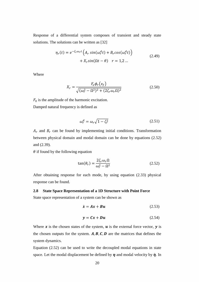
Response of a differential system composes of transient and steady state

solutions. The solutions can be written as [32]

𝜂𝑟(𝑡) = 𝑒−𝜁𝑟𝜔𝑟𝑡 (𝐴𝑟 𝑠𝑖𝑛(𝜔𝑟

𝑑𝑡) + 𝐵𝑟𝑐𝑜𝑠(𝜔𝑟𝑑𝑡))

+ 𝑋𝑟𝑠𝑖𝑛(Ω𝑡 − 𝜃) 𝑟 = 1,2…

(2.49)

Where

𝑋𝑟 =𝐹𝑜𝜙𝑟(𝑥𝑓)

√(𝜔𝑟2 − Ω2)2 + (2𝜁𝑟𝜔𝑟Ω)2

(2.50)

𝐹0 is the amplitude of the harmonic excitation.

Damped natural frequency is defined as

𝜔𝑟𝑑 = 𝜔𝑟√1 − 𝜁𝑟

2 (2.51)

𝐴𝑟 and 𝐵𝑟 can be found by implementing initial conditions. Transformation

between physical domain and modal domain can be done by equations (2.52)

and (2.39).

𝜃 if found by the following equation

tan(𝜃𝑟) =2𝜁𝑟𝜔𝑟Ω

𝜔𝑟2 − Ω2

(2.52)

After obtaining response for each mode, by using equation (2.33) physical

response can be found.

2.8 State Space Representation of a 1D Structure with Point Force

State space representation of a system can be shown as

�̇� = 𝑨𝒙 + 𝑩𝒖 (2.53)

𝒚 = 𝑪𝒙 + 𝑫𝒖 (2.54)

Where 𝒙 is the chosen states of the system, 𝒖 is the external force vector, 𝒚 is

the chosen outputs for the system. 𝑨,𝑩, 𝑪,𝑫 are the matrices that defines the

system dynamics.

Equation (2.52) can be used to write the decoupled modal equations in state

space. Let the modal displacement be defined by 𝜼 and modal velocity by �̇�. In

21

the previous analysis it is shown that the response of a structure is infinite sum

of its modal domain SDOF responses. However, in real case it is necessary to

truncate it to a finite number of modes. Let the number of modes used in the

series summation is 𝑚 and number of forces are 𝑓. Then, states and their

derivatives can be written respectively as

𝒙 = [𝜂1 𝜂2 …𝜂𝑚 �̇�1 �̇�2 … �̇�𝑚]2𝑚𝑥1𝑇 (2.55)

�̇� = [�̇�1 �̇�2 … �̇�𝑚 �̈�1 �̈�2 … �̈�𝑚 ]2𝑚𝑥1𝑇 (2.56)

The normalized mode shape functions are defined as

𝚽(𝒙) = [𝝓𝟏(𝒙) 𝝓𝟐(𝒙) … 𝝓𝒎(𝒙)]1𝑥𝑚 (2.57)

Considering equation (2.52) and re-writing it in the appropriate format

𝜂�̈�(𝑡) = −2𝜔𝑟𝜁𝑟�̇�(𝑡) − 𝜔𝑟

2𝜂𝑟(𝑡) + 𝜙𝑟(𝑥1)𝐹1(𝑡) + 𝜙𝑟(𝑥2)𝐹2(𝑡)

+ ⋯+ 𝜙𝑟(𝑥𝑓)𝐹𝑓(𝑡), 𝑟 = 1,2 (2.58)

Then the A and B matrices can be written as

𝑨 = [𝟎𝑚𝑥𝑚 𝑰𝑚𝑥𝑚

−𝝎𝒎𝒙𝒎𝟐 −𝟐𝜻𝝎𝒎𝒙𝒎

]2𝑚𝑥2𝑚

(2.59)

𝑩 = [𝟎𝑚𝑥𝑓

𝛷𝑇(𝑥1) 𝛷𝑇(𝑥2)…𝛷𝑇(𝑥𝑓)

]2𝑚𝑥𝑓

(2.60)

And 𝜔2 , −2𝜁𝜔 and u can be written as

𝒖 = [𝐹1(𝑡) 𝐹2(𝑡)…𝐹𝑓(𝑡)]𝑓𝑥1

𝑇 (2.61)

𝝎𝟐 =

[ 𝜔1

2 0 … 0

0 𝜔22 … …

… … … 00 … 0 𝑤𝑚

2 ]

𝑚𝑥𝑚

(2.62)

−𝟐𝜻𝝎 = [

−2𝜁1𝜔1 0 … 00 −2𝜁2𝜔2 … …… … … 00 … 0 −2𝜁𝑚𝑤𝑚

]

𝑚𝑥𝑚

(2.63)

22

This concludes the definition of 𝑨 and 𝑩 matrices. Outputs are the displacement,

velocity or acceleration of an arbitrary point defined in the domain of the

structure. Then to find the displacements, equation (2.33) is re-written.

𝑦(𝑥, 𝑡) = ∑𝜙𝑟(𝑥)𝜂𝑟(𝑡)

∞

𝑟=1

(2.64)

Taking the derivative with respect to time will yield the velocity of a point.

�̇�(𝑥, 𝑡) = ∑𝜙𝑟(𝑥)�̇�𝑟(𝑡)

∞

𝑟=1

(2.65)

It is possible to write y(x,t) and �̇�(𝑥, 𝑡) in terms of the states 𝜂, �̇�. To find the

acceleration one more derivative is taken with respect to time.

�̈�(𝑥, 𝑡) = ∑𝜙𝑟(𝑥)�̈�𝑟(𝑡)

∞

𝑟=1

(2.66)

�̈� is not one of the states. Then it is necessary to write it in terms of 𝜼 𝑎𝑛𝑑 �̇� .

From equation (2.53) it is known that

𝜂�̈�(𝑡) = −2𝜁𝑟𝜔𝑟 − 𝜔𝑟

2𝜂𝑟(𝑡) + 𝜙𝑟(𝑥1)𝐹1(𝑡) + 𝜙𝑟(𝑥2)𝐹2(𝑡) + ⋯

+ 𝜙𝑟(𝑥𝑓)𝐹𝑓(𝑡), 𝑟 = 1,2 (2.67)

Then placing (2.58) into (2.66) the acceleration can be found in terms of our

states and external excitations. To find the 𝑦 given below, the 𝑪 and 𝑫 matrix

can be written in general form as

𝒚𝒌 = [𝑦(𝑥𝑘, 𝑡) �̇�(𝑥𝑘, 𝑡) �̈�(𝑥𝑘, 𝑡)]𝑇 (2.68)

𝐂 = [

𝚽(𝐱𝐤)𝟏𝐱𝐦 𝟎𝟏𝐱𝐦

𝟎𝟏𝐱𝐦 𝚽(𝐱𝐤)𝟏𝐱𝐦

−𝛚𝟐𝚽(𝐱𝐤)𝟏𝐱𝐦 −𝟐𝛇𝛚𝚽(𝐱𝐤)𝟏𝐱𝐦

]

𝟑x2m

(2.69)

𝑫 = [

𝟎𝟏𝒙𝒇

𝟎𝟏𝒙𝒇

𝛷(𝑥𝑘)1𝑥𝑚[𝛷𝑇(𝑥1) 𝛷𝑇(𝑥2)…𝛷𝑇(𝑥𝑓)]𝑚𝑥𝑓

]

3𝑥𝑓

(2.70)

23

2.9 Numerical Example

2.9.1 Problem Definition

The state space representation with 5 modes will be compared with the analytical

formulation result with 5 modes of a simply supported beam with the following

properties

Length: 1 meter

Width: 0.1 meters

Height: 0.01 meters

Excitation point, xf = 0.3 meter

Excitation frequency: Ω = 10 Hz, 50 Hz

Required response is at x = 0.5 meter

Damping: 5% to each mode

Number of modes: 5

Then the required parameters can be calculated as

L = 1 m

E = 70 GPa

I = 8.33x 10-9 m4

m = 2.7 kg/m

The normalized mode shapes for simply supported beam are

𝜙𝑟(𝑥) = √2

𝑚𝐿𝑠𝑖𝑛

𝑟𝜋𝑥

𝐿, 𝑟 = 1,2, … ,𝑚

The natural frequencies are

𝜔𝑟 = (𝑟𝜋)2√𝐸𝐼

𝑚𝐿4

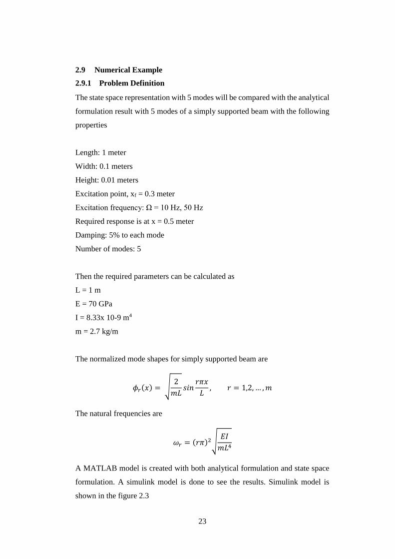
A MATLAB model is created with both analytical formulation and state space

formulation. A simulink model is done to see the results. Simulink model is

shown in the figure 2.3

24

Figure 2-3 - Simulink Model of Open Loop State Space System

As 5 modes are modelled in the simulation, one should determine the step size

accordingly. 5th mode is at 577 Hz, then a step size of 10-4 is selected. For

analytical model directly MATLAB is used. For state space model fixed-step

size ode8 solver is used.

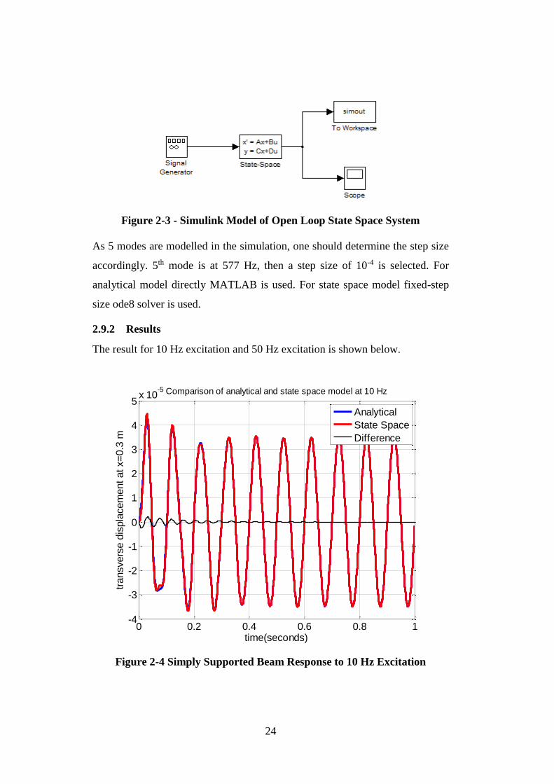
2.9.2 Results

The result for 10 Hz excitation and 50 Hz excitation is shown below.

Figure 2-4 Simply Supported Beam Response to 10 Hz Excitation

0 0.2 0.4 0.6 0.8 1-4

-3

-2

-1

0

1

2

3

4

5x 10

-5

time(seconds)

transvers

e d

ispla

cem

ent at x=

0.3

m

Comparison of analytical and state space model at 10 Hz

Analytical

State Space

Difference

25

Figure 2-5 Simply Supported Beam Response to 50 Hz Excitation

2.10 Numerical Example II

By applying step input and waiting appropriate time to damp out transient

response one should obtain steady state static deflection. Also static deflection

of a simply supported beam is also analytically known From [33] for an

intermediate load the scheme is

Figure 2-6 Simply Supported Beam Intermediate Load Static Deflection

0 0.2 0.4 0.6 0.8 1-2

-1.5

-1

-0.5

0

0.5

1

1.5

2

2.5x 10

-5

time(seconds)

transvers

e d

ispla

cem

ent at x=

0.3

m

Comparison of analytical and state space model at 50 Hz

Analytical

State Space

Difference

26

And for the deflection between B and C is defined as

𝑦 =𝐹𝑎(𝑙 − 𝑥)

6𝐸𝐼𝑙(𝑥2 + 𝑎2 − 2𝑙𝑥) (2.71)

The geometry, boundary conditions and material is same as the Section 2.8. A

step force is applied at 0.3 meters and the deflection at 0.5 meters is sought. Then

𝑎 = 0.3 𝑚, 𝑥 = 0.5 𝑚, 𝐹 = 1𝑁, 𝑙 = 1 𝑚, 𝐸𝐼 = 583.1 𝑁𝑚2

Then by placing the values the deflection is found as

𝑦 = −2.8297 ∗ 10−5 𝑚

Simply supported beam with same properties and same force properties is

modelled in Matlab and simulated by Simulink. The state space result is given

in Figure 2-6. The steady state response is 2.828 ∗ 10−5 𝑚 and error between

analytical formulation and state space representation is 0.06%.

Figure 2-7 Simply Supported Beam Response to Step Input and Steady

State Result

0 0.1 0.2 0.3 0.4 0.5 0.6 0.7 0.8 0.9 1-1

0

1

2

3

4

5

6x 10

-5

time(seconds)

transvers

e d

ispla

cem

ent

at

x=

0.5

m

27

CHAPTER 3

DISCRETIZATION AND GENERALIZATION OF STATE SPACE

MODEL

3.1 Introduction

In Chapter 2 it is shown that a distributed structure can be modelled in state space

as the sum of its normalized modes. It is possible to model rods, strings, beams

and plates with the analytical models that are available in the literature.

However, most of the structures that are used in real life does not have any

analytical model. To overcome this problem, Finite Element Analysis (FEA) is

widely used. In FEA a structure is divided into finite number of structural

elements and the solution for displacement, velocity, temperature etc. is found

numerically. In our case it is required to find mode shape vectors, natural

frequencies, modal masses and modal stiffnesses.

3.2 Discretizing the 1D State Space Model

Only difference between distributed model and discrete model is in terms of

mode shape definition. In continuous analysis mode shapes are functions that are

expressed analytically. In the discretized structures mode shape vectors are used.

The vectors are analogous to continuous shape functions, in fact the values are

pre-calculated at nodes of the structure.

In Chapter 2, it is shown that for the case with excitation using point forces it is

possible to obtain a state space model. To prevent interpolations in discrete

modelling, it is assumed that forces are applied to the nodes of the FEM.

Furthermore, the responses are also calculated at the nodes. With the above

differences in mind, 𝑨,𝑩, 𝑪,𝑫 matrices should be rewritten for a discrete case.

The definition for the mode shape vector for rth mode is given as

𝝓𝒓 = [𝜙𝑟(1) 𝜙𝑟(2)…𝜙𝑟(𝑛)]𝑛𝑥1𝑇 (3.1)

Where 𝑛 is the number of nodes in the structure. The mode shape matrix is

written as

𝚽 = [𝝓𝟏 𝝓𝟐 …𝝓𝒎]𝑛𝑥𝑚 (3.2)

28

Where m is the number of modes included in the model. Then considering the

same process given in Section 2.7 𝑨, 𝑩, 𝑪,𝑫 are the same. However it is

necessary to choose the points such that they are coincident with the nodes of

the FEA. Also it should be noted that

𝚽(𝒙) = [𝝓𝟏(𝒙) 𝝓𝟐(𝒙)…𝝓𝒎(𝒙)]1𝑥𝑚 (3.3)

And 𝑥 is the selected node number. Therefore instead of using physical

coordinates to evaluate mode shape function now the values directly at the

selected node is used the equations.

3.3 Generalized State Space Approach in 3D

In the literature survey it is shown that modal space approach is used on

cantilever beams and plate type structures. However it is not common to use this

approach for three dimensional structures. The formulation given in Section 3-1

and 3.3 will be expanded for three dimensional structures in this section.

In addition to m and n, the number of modes included in the model and number

of nodes of FEA, a new abbreviation d is added to the formulation which is the

number of degrees of freedom of a structure. It is taken as six in the formulation

as a point can translate in three directions and can rotate about three axes.

Mode shape vector is written in the form given in Eqn. 3.4. Subscripts denote

the mode number and superscripts denotes the mode shape vector at that degree

of freedom.

𝝓𝒊 =

[

𝜙𝑖𝑥

𝜙𝑖𝑦

𝜙𝑖𝑧

𝜙𝑖𝑟𝑜𝑡𝑥

𝜙𝑖𝑟𝑜𝑡𝑦

𝜙𝑖𝑟𝑜𝑡𝑧]

(𝑑∗𝑛)𝑥1

(3.4)

And the mode shape matrix is written as

𝚽 = [𝝓𝟏 𝝓𝟐 …𝝓𝒎−𝟏𝝓𝒎](𝑑∗𝑛)𝑥𝑚 (3.5)

States are same as before, modal displacements and modal velocities.

29

𝒙 = [𝜂1 𝜂2 …𝜂𝑚 �̇�1 �̇�2 … �̇�𝑚]2𝑚𝑥1𝑇 (3.6)

𝑨 matrix is same as before as it does not include any mode shapes term. Only

natural frequencies and modal damping ratios are included.

𝑩 matrix is expanded to include all the information about every node. To find 𝑩

matrix we need to first obtain input vector 𝒖. At every node, three forces and

three moments can be applied. Therefore the size of the matrix is d*n x 1.

Subscripts denote the node number and superscripts denote the degree of

freedom. 𝐹 is for forces and 𝑀 is for moments.

𝒖

= [𝐹1𝑥. . 𝐹𝑛

𝑥 𝐹1𝑦. . 𝐹𝑛

𝑦 𝐹1

𝑧 . . 𝐹𝑛𝑧 𝑀1

𝑥. . 𝑀𝑛𝑥 𝑀1

𝑦. . 𝑀𝑛

𝑦. . 𝑀1

𝑧 . . 𝑀𝑛𝑧]

𝑑𝑛 𝑥 1

𝑇

(3.7)

𝑩 =

[ 𝟎𝒎𝒙𝟏

𝝓𝟏𝑻

𝝓𝟐𝑻

…𝝓𝒎−𝟏

𝑻

𝝓𝒎𝑻 ]

(2𝑚) 𝑥 (𝑑𝑛)

(3.8)

𝒚 vector is the output vector. It contains the information of displacement,

velocity and acceleration of every node in every direction. (6 degrees of

freedom). Therefore the number of elements in it is 3*n*d. Its dimensions are

(3*n*d) x 1. The coding is given below. Subscripts are used for node number.

𝒙 = [𝑥1 𝑥2 …𝑥𝑛]𝑇𝑛𝑥1

�̇� = [𝑥1̇ 𝑥2̇ …𝑥�̇�]𝑇𝑛𝑥1

�̈� =

[𝑥1̈ 𝑥2̈ …𝑥�̈�]𝑛𝑥1

𝒚 = [𝑦1 𝑦2 …𝑦𝑛]𝑇𝑛𝑥1

�̇� = [𝑦1̇ 𝑦2̇ …𝑦�̇�]𝑇𝑛𝑥1

�̈� =

[𝑦1̈ 𝑦2̈ …𝑦�̈�]𝑛𝑥1

𝒛 = [𝑧1 𝑧2 …𝑧𝑛]𝑇𝑛𝑥1

�̇� = [𝑧1̇ 𝑧2̇ …𝑧�̇�]𝑇𝑛𝑥1

�̈� =

[𝑧1̈ 𝑧2̈ …𝑧�̈�]𝑛𝑥1

(3.9a-3.9i)

30

𝒓𝒐𝒕𝒙 = [𝑟𝑜𝑡𝑥1 𝑟𝑜𝑡𝑥2 …𝑟𝑜𝑡𝑥𝑛]𝑇𝑛𝑥1

(3.10a)

𝒓𝒐𝒕𝒙̇ = [𝑟𝑜𝑡𝑥1̇ 𝑟𝑜𝑡𝑥2̇ … 𝑟𝑜𝑡𝑥𝑛̇ ]𝑇𝑛𝑥1

(3.10b)

𝒓𝒐𝒕𝒙̈ = [𝑟𝑜𝑡𝑥1̈ 𝑟𝑜𝑡𝑥2̈ … 𝑟𝑜𝑡𝑥𝑛̈ ]𝑛𝑥1 (3.10c)

𝒓𝒐𝒕𝒚 = [𝑟𝑜𝑡𝑦1 𝑟𝑜𝑡𝑦2 …𝑟𝑜𝑡𝑦𝑛]𝑇𝑛𝑥1

(3.10d)

𝒓𝒐𝒕𝒚̇ = [𝑟𝑜𝑡𝑦1̇ 𝑟𝑜𝑡𝑦2̇ … 𝑟𝑜𝑡𝑦𝑛̇ ]𝑇𝑛𝑥1

(3.10e)

𝒓𝒐𝒕𝒚̈ = [𝑟𝑜𝑡𝑦1̈ 𝑟𝑜𝑡𝑦2̈ … 𝑟𝑜𝑡𝑦𝑛̈ ]𝑛𝑥1 (3.10f)

𝒓𝒐𝒕𝒛 = [𝑟𝑜𝑡𝑧1 𝑟𝑜𝑡𝑧2 …𝑟𝑜𝑡𝑧𝑛]𝑇𝑛𝑥1

(3.10g)

𝒓𝒐𝒕𝒛̇ = [𝑟𝑜𝑡𝑧1̇ 𝑟𝑜𝑡𝑧2̇ … 𝑟𝑜𝑡𝑧𝑛̇ ]𝑇𝑛𝑥1

(3.10h)

𝒓𝒐𝒕𝒛̈ = [𝑟𝑜𝑡𝑧1̈ 𝑟𝑜𝑡𝑧2̈ … 𝑟𝑜𝑡𝑧𝑛̈ ]𝑛𝑥1 (3.10i)

𝒀 =

[

𝒙𝒚𝒛

𝒓𝒐𝒕𝒙𝒓𝒐𝒕𝒚𝒓𝒐𝒕𝒛]

(𝑑∗𝑛) 𝑥 1

�̇� =

[

�̇��̇��̇�

𝒓𝒐𝒕𝒙̇

𝒓𝒐𝒕𝒚̇

𝒓𝒐𝒕𝒛̇ ]

(𝑑∗𝑛) 𝑥 1

�̈� =

[

�̈��̈��̈�

𝒓𝒐𝒕𝒙̈

𝒓𝒐𝒕𝒚̈

𝒓𝒐𝒕𝒛̈ ]

(𝑑∗𝑛) 𝑥 1

(3.11)

𝒚 = [𝒀�̇��̈�]

(3∗𝑑∗𝑛) 𝑥 1

(3.12)

With the given 𝒚 vector 𝑪 and 𝑫 matrices can be revised. The total

displacements, velocities and accelerations can be obtained by modal

superposition. Superposition is shown below.

𝑦(𝑥1, 𝑡) = 𝜙1(𝑥1)𝜂1(𝑡) + 𝜙2(𝑥1)𝜂2(𝑡) + ⋯+ 𝜙𝑚−1(𝑥1)𝜂𝑚−1(𝑡)

+ 𝜙𝑚(𝑥1)𝜂𝑚(𝑡)

�̇�(𝑥1, 𝑡) = 𝜙1(𝑥1)𝜂1̇(𝑡) + 𝜙2(𝑥1)𝜂2̇(𝑡) + ⋯+ 𝜙𝑚−1(𝑥1)𝜂𝑚−1̇ (𝑡)

+ 𝜙𝑚(𝑥1)𝜂�̇�(𝑡)

31

�̈�(𝑥1, 𝑡) = 𝜙1(𝑥1)𝜂1̈(𝑡) + 𝜙2(𝑥1)𝜂2̈(𝑡) + ⋯+ 𝜙𝑚−1(𝑥1)𝜂𝑚−1̈ (𝑡)

+ 𝜙𝑚(𝑥1)𝜂�̈�(𝑡)

(3.13a-3.13c)

By expanding this to matrix form

𝒀 = 𝝓[𝜂1 𝜂2 …𝜂𝑚]𝑇 (3.14)

As velocities are also out states

�̇� = 𝝓[𝜂𝑚+1 𝜂𝑚+2 …𝜂2𝑚]𝑇 (3.15)

To find accelerations firstly rewrite the modal equation

�̈�𝑟(𝑡) = −2𝜔𝑟𝜁𝜂�̇�(𝑡) − 𝜔𝑟2𝜂𝑟(𝑡) + 𝜙𝑟(𝑥𝑓)𝐹𝑟(𝑡) (3.16)

Revise the forcing section to be general similar to u vector at (3.7) contains all

the forces and moments.

�̈�𝑟(𝑡) = −2𝜔𝑟𝜁𝜂�̇�(𝑡) − 𝜔𝑟2𝜂𝑟(𝑡) + 𝜙𝑟

𝑇𝑢(𝑡) (3.17)

Then multiplying (3.17) with 𝝓 will give the accelerations. From here 𝑪 and 𝑫

matrices can be obtained as following.

𝑪 = [

𝚽 𝟎𝒅𝒏𝒙𝒎

𝟎𝒅𝒏𝒙𝒎 𝚽

−𝚽𝝎𝟐 −𝟐𝚽𝜻𝝎]

3𝑑𝑛𝑥2𝑚

(3.18)

𝑫 = [𝟎𝒅𝒏𝒙𝒅𝒏

𝟎𝒅𝒏𝒙𝒅𝒏

𝚽𝚽𝑻

]

3𝑑𝑛𝑥𝑑𝑛

(3.19)

With those 𝑨,𝑩, 𝑪, and 𝑫 matrices any structure with 3D FEA can be modeled

in state space.

3.4 Reducing the size of B, C, D Matrices

Calculated 𝑩, 𝑪,𝑫 matrices obtain data about every node. However in real case

information on 𝑩 matrix should only contain the actuated node and 𝑪 & 𝑫

matrices should only contain information of the nodes with sensors. Then

controllability and observability matrices can be correctly found.

32

Assuming there are 𝑓 number of actuators. 𝑩 matrix should reduce from (2m

x dn) to (2m x f) size such that 𝒖 vector is size of (f x 1). Then to eliminate the

unnecessary information from 𝑩 matrix, lower side of 𝑩 matrix is multiplied

with a matrix 𝑬𝒇 size of (dn x f). 𝑬𝒇 is a 0 matrix except 1 is placed at

(d(w)*n(w),w), where w stands for point forces starting from 1 to f. d(w) stands

for the corresponding degree of freedom of the actuator and n is the

corresponding node number. 𝑩 matrix is written as

𝑩 = [𝟎𝒎𝒙𝟏

𝚽𝑻 ∗ 𝑬𝒇](2𝑚) 𝑥 (𝑓)

(3.20)

Similar approach can be done for 𝑪 and 𝑫 matrices. Assume that 𝑑𝑖𝑠 is the

number of displacement sensors, 𝑣𝑒𝑙 is the number of velocity sensors and 𝑎𝑐𝑐

is the number of acceleration sensors. 𝑬𝒅, 𝑬𝒗, 𝑬𝒂 are the corresponding matrices

with size of (dis x d*n), (vel x d*n), (acc x d*n). 𝑪 and 𝑫 matrices can be written

at reduced form as

𝑪 = [

𝐄𝐝𝚽 𝟎𝒅𝒏𝒙𝒎

𝟎𝒅𝒏𝒙𝒎 𝐄𝐯𝚽

−𝑬𝒂𝚽𝝎𝟐 −𝑬𝒂𝟐𝚽𝜻𝝎]

(𝑑𝑖𝑠+𝑣𝑒𝑙+𝑎𝑐𝑐)𝑥2𝑚

(3.21)

𝑫 = [

𝟎𝒅𝒊𝒔𝒙𝒅𝒏

𝟎𝒗𝒆𝒍𝒙𝒅𝒏

𝐄𝐝𝚽𝚽𝑻𝑬𝒂

]

(𝑑𝑖𝑠+𝑣𝑒𝑙+𝑎𝑐𝑐)𝑥𝑑𝑛

(3.22)

𝑬𝒅 is a zero matrix except (@dis, d(@dis)*n(@dis)) = 1. @dis corresponds for

the number of the sensor from 1 to dis and d(@dis) gives the degree of freedom

displacement sensor and n(@dis) gives the node of displacement sensor. 𝑬𝒗 and

𝑬𝒂 sensors can be found with same procedure for velocity and acceleration

sensors.

3.5 Discrete Simply Supported Beam Compared With the Continuous

Model

For the same beam given in Section 2.8 a finite element analysis has been done

using NASTRAN/PATRAN. Beam is discretized into 20 one dimensional beam

33

elements with 21 nodes. Each node is uniformly distributed from each other.

Length of the beam is 1 meter. Distance between nodes are 0.05 m. This suggests

that one must choose the actuator points or sensor points at those intervals. The

nodes of the beam are shown in Figure 3.1 below.

Figure 3-1 Simply Supported Beam Model and Node Numbers

One dimensional modal analysis is performed using FEM and the resulting mode

shapes for first three modes are shown in the Figures 3-2 to 3-4. The number on

each figure indicates the maximum value for displacement ratio. The mode

shapes are mass normalized.

Figure 3-2 First Mode Shape

Figure 3-3 Second Mode Shape

Figure 3-4 Third Mode Shape

For the first eight modes, the natural frequencies are compared with the

distributed model in the Table 3.1.

34

Table 3-1 Comparison of Natural Frequencies for Simply Supported Beam

Discrete Model (Hz) Distributed Model (Hz)

1st mode 23.086 23.088

2nd mode 92.306 92.354

3rd mode 207.55 207.80

4th mode 368.6 369.4

5th mode 575.12 577.2

6th mode 826.57 831.2

7th mode 1122.11 1131.33

8th mode 1460.6 1477.66

The error is increasing as the modes increase however up to seventh mode

absolute error is below 1% and at eighth mode absolute error is 1.15%. In the

previous corresponding example, excitation was applied at x=0.3m and response

was measured at x=0.5m. Then the mode shape values at those points should be

compared with each other before comparing the results. Then for x=0.3m values

at seventh node will be taken and compared with continuous model.

Table 3-2 Comparison of Mode Shape Values of Simply Supported Beam

Discrete Model - 𝜙(7) Distributed Model

𝜙(0.3)

1st mode 0.696291 0.696290

2nd mode 0.818539 0.818539

3rd mode 0.26596 0.26595

4th mode -0.505885 -0.505884

5th mode -0.86066 -0.86066

6th mode -0.50589 -0.50588

7th mode 0.26596 0.26595

8th mode 0.81854 0.81853

35

Results are accurate up to 4 digits. Then the same procedure is repeated for

x=0.5m. The results are shown in the Table 3.3

Table 3-3 Comparison of Mode Shape Values of Simply Supported Beam

Discrete Model - 𝜙(11) Distributed Model

𝜙(0.5)

1st mode -0.860663 - 0.860662

2nd mode 0 0

3rd mode 0.860663 0.860662

4th mode 0 0

5th mode 0.860663 0.860662

6th mode 0 0

7th mode -0.86066 -0.860662

8th mode 0 0

The natural frequencies and mode shapes at the given locations are very close to

each other. Then it is expected to have similar results. MATLAB and Simulink

is used for simulations. 10-4 fixed step size is given. For Simulink solution ode5

solver is used. 5% damping is added to the every mode. 8 modes are used, which

is up to 1477 Hz.

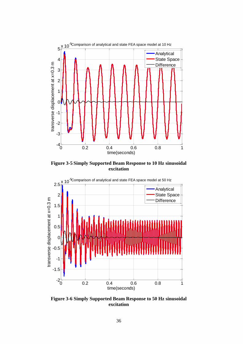
10 Hz and 50 Hz excitations are considered separately. The results are given

below. Difference is the error between Analytical Response and State Space

Response

36

Figure 3-5 Simply Supported Beam Response to 10 Hz sinusoidal

excitation

Figure 3-6 Simply Supported Beam Response to 50 Hz sinusoidal

excitation

0 0.2 0.4 0.6 0.8 1-4

-3

-2

-1

0

1

2

3

4

5x 10

-5

time(seconds)

transvers

e d

ispla

cem

ent at x=

0.3

m

Comparison of analytical and state FEA space model at 10 Hz

Analytical

State Space

Difference

0 0.2 0.4 0.6 0.8 1-2

-1.5

-1

-0.5

0

0.5

1

1.5

2

2.5x 10

-5

time(seconds)

transvers

e d

ispla

cem

ent at x=

0.3

m

Comparison of analytical and state FEA space model at 50 Hz

Analytical

State Space

Difference

37

In Figure 3-6 it can be seen that FEA result transient and steady state part is in

good agreement with analytical response.

3.6 Numerical Example for Complex Structure

To better evaluate the performance of the state space model, a three dimensional

complex shape will be used as a case study. The structure is shown below with

the node numbers. The selection of the shape is due to its three dimensional

nature. It is modelled with five modes (m=5) 236 nodes (n=236) and three

translational degrees of freedom (d=3). It is fixed from the edge of nodes

between 1 and 11.

Figure 3-7 Three dimensional complex structure with node numbers

The structure is an aluminum with Young’s modulus 70 GPa, density 2700 kg/m3

and it has a thickness of 2 mm. The long sides are 100 mm and short sides are

50 mm. The first three mode shapes are given below to better visualize the

dynamics of the system.

38

1st mode

2nd mode

3rd mode

Figure 3-8 First three mode shapes of complex structure

Then assuming that there is an excitation from node 120 in Z direction and

accelerometers are located at node 130 in Y direction and at 235 in X direction.

The natural frequencies of the system is given in Table 3.4.

39

Table 3-4 Natural Frequencies of the complex structure

1st mode 48.917 Hz

2nd mode 98.345 Hz

3rd mode 156.46 Hz

4th mode 324.06 Hz

5th mode 619.55 Hz

From here state space matrices 𝑨,𝑩, 𝑪, and 𝑫 can be constructed.

A matrix

Assuming that there exists 1% damping for first mode, 2% for second mode and

m% for mth mode, diagonal natural frequency and diagonal damping sub-

matrices will be defined first.

The natural frequencies of the structure from FEA is shown in Table 3.4 in the

form of Hz. It is necessary to convert them to rad/sec and square them. Then the

diagonal natural frequency matrix can be found and written below as

𝝎𝟐

=

[ 9.4467𝑒 + 004 0 0 0 0

0 3.8182𝑒 + 005 0 0 00 0 9.6642𝑒 + 005 0 00 0 0 4.1458𝑒 + 006 00 0 0 0 1.5153𝑒 + 007]

Also,

𝟐𝝎𝜻 =

[ 6.1471 0 0 0 0

0 24.7168 0 0 00 0 58.9840 0 00 0 0 162.8903 00 0 0 0 389.2747]

and I is 5x5 identity matrix and 0 is 5x5 null matrix. Then A is

𝑨 = [𝟎 𝑰

−𝝎𝟐 −𝟐𝝎𝜻]

B matrix

To define the 𝑩 matrix, the mode shape values at the 120th node in Z direction

must be known first.

40

Table 3-5 Mode shape values at excitation point

Mode Number Mode Shape Value at node 120 in Z

direction

1st mode -2.013535

2nd mode 2.597269

3rd mode 3.264399

4th mode 1.182970

5th mode 14.493186

The forcing function u(t) is defined as

𝑢(𝑡) = 𝑓1(𝑡)

As f1 is an arbitrary input force. B matrix can be written considering Table 3.5.

𝑩 =

[

00000

−2.0135352.5972693.2643991.18297014.493186]

C matrix

To define the 𝑪 matrix, the mode shape values of node 130 in Y direction and

node 235 in X direction should be written.

41

Table 3-6 Mode shape values at sensor points

Mode Number Mode Shape Value at

130th node Y

direction

Mode Shape Value at

235th node X direction

1st mode 4.758248 -0.303674

2nd mode -0.188935 -7.200803

3rd mode 4.694722 -0.890994

4th mode 8.892684 8.593676

5th mode -2.919328 1.375139

𝝓𝒄 = [4.76 −0.19 4.69 8.89 −2.91

−0.30 −7.20 −0.89 8.59 1.38]

Then to find the C matrix one should multiply 𝝓𝒄 with −𝝎𝟐 𝑎𝑛𝑑 − 𝟐𝝎𝜻 which

are given in the A matrix formulation. Formulation of 𝑪 matrix can be shown for

accelerometer type sensors as

𝑪 = [−𝝓𝒄𝝎𝟐 −𝝓𝒄(𝟐𝝎𝜻)]

Then the result for this case is

𝑪𝟏 = −𝝓𝒄𝝎𝟐 = 1𝑒7 [

−0.0450 0.0073 −0.4533 −3.6856 4.40970.0028 0.2749 0.0860 −3.5613 −2.0912

]

𝑪𝟐 = −𝝓𝒄(𝟐𝝎𝜻)

= 1𝑒3 [−0.0293 0.0047 −0.2766 −1.4481 1.13280.0018 0.1780 0.0525 −1.3992 −0.5372

]

𝑪 = [𝑪𝟏 𝑪𝟐]

D matrix

The mode shape functions necessary for 𝑫 matrix calculations are already given.

𝑫 matrix is mathematically defined for accelerometer sensors as

𝑫 = [𝝓𝒔𝝓𝒇𝑻]

Where 𝝓𝒔 is the mode shape values at the sensor locations which are given at

𝝓𝒄 actually, and 𝝓𝒇𝑻 is the mode shape values at the excitation locations which

42

is actually lower half of the B matrix. Then D matrix is calculated for our case

as

𝑫 = [−26.459.11

]

3.7 Comparison of FEA and State Space Model for Complex Structure

To verify the model state space representation of 3D structure is compared with

the transient response results of NATRAN/PATRAN software. 10 modes are

modelled and 5% damping is given to each mode. Then step input of 1N is

applied to the given locations. Response from the same point is measured and

compared. A step input is given in the Y axis. The structure is fixed from the

lower side shown with filled rectangle.

The results and errors are drawn in the figure 10 and figure 11. It can be seen

that error is around 0.1%. Also a sine input of 10Hz with 1N amplitude is given

from node 235 in X axis shown in figure 12. The results and error rate can be

found in the figure 13 and figure 14 respectively. Error is around 3%.

Figure 3-9 Complex Structure Step Input from Y Axis

43

Figure 3-10 – Comparison of FEA and SS Responses to Step Input

Figure 3-11 Error Percentage between FEA and SS Response to Step

Input

0 0.1 0.2 0.3 0.4 0.5 0.6 0.7 0.8 0.9 10

1

2

3

4

5

6x 10

-4

time(seconds)

Response (

mete

rs)

Response to Step Input

FEA

SS

0 0.1 0.2 0.3 0.4 0.5 0.6 0.7 0.8 0.9 1-0.1

-0.05

0

0.05

0.1

0.15

time(seconds)

Err

or

%

Relative Error between FEA and State Space Model

44

Figure 3-13 Comparison of SS and FEA Responses to Sinusoidal

Disturbance

0 0.2 0.4 0.6 0.8 1 1.2 1.4 1.6 1.8 2-2

-1

0

1

2x 10

-4

time(seconds)

Response (

mete

rs)

Response to 10 Hz Input

FEA

SS

Figure 3-12 Complex Structure Sinusoidal Input from Y Axis

45

Figure 3-14 Error Percentage between FEA and SS Response to

Sinusoidal Input

0 0.5 1 1.5 2 2.5 3-4

-3

-2

-1

0

1

2

3

4

time(seconds)

Err

or

%

Relative Error between FEA and State Space Model

46

47

CHAPTER 4

MODAL SPACE CONTROL IN STATE SPACE

4.1 Introduction

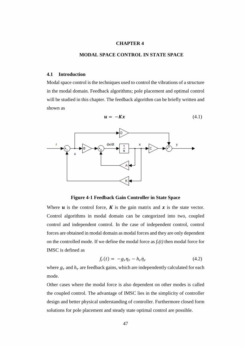
Modal space control is the techniques used to control the vibrations of a structure

in the modal domain. Feedback algorithms; pole placement and optimal control

will be studied in this chapter. The feedback algorithm can be briefly written and

shown as

𝒖 = −𝑲𝒙 (4.1)

Figure 4-1 Feedback Gain Controller in State Space

Where 𝒖 is the control force, 𝑲 is the gain matrix and 𝒙 is the state vector.

Control algorithms in modal domain can be categorized into two, coupled

control and independent control. In the case of independent control, control

forces are obtained in modal domain as modal forces and they are only dependent

on the controlled mode. If we define the modal force as fr(t) then modal force for

IMSC is defined as

𝑓𝑟(𝑡) = −𝑔𝑟𝜂𝑟 − ℎ𝑟�̇�𝑟 (4.2)

where 𝑔𝑟 and ℎ𝑟 are feedback gains, which are independently calculated for each

mode.

Other cases where the modal force is also dependent on other modes is called

the coupled control. The advantage of IMSC lies in the simplicity of controller

design and better physical understanding of controller. Furthermore closed form

solutions for pole placement and steady state optimal control are possible.

48

The coefficients g and h will be found separately for pole placement and optimal

control. Before that, the connection between modal force and real forces will be

shown. For point forces the relation between modal force and real force is

𝒇(𝒕) = 𝑩𝑳𝑭(𝒕) (4.3)

Where 𝑩𝑳 is the lower half of 𝑩 matrix, 𝒇(𝒕)is modal force and 𝑭(𝒕) is real

force. Having 𝑓 number of actuators and 𝑚 modes the size of the matrix 𝑩𝑳 is

(fxm). 𝑩𝑳 does not have to be a square matrix but if that is the case a pseudo-

inverse will be necessary to calculate the real forces 𝑭(𝒕).

𝑭(𝒕) = 𝑩𝑳+𝒇(𝒕) (4.4)

And placing (4.2) into (4.4) K can be obtained as

𝑲 = 𝑩𝑳+[−𝑮𝜼(𝒕) − 𝑯�̇�(𝒕)] (4.5)

Where G and H are diagonal gain matrices with the respective coefficients for

each mode. In the above expression + is used for pseudo inverse operation. If the

number of modes is equal to number of actuators (i.e. m=f) then the pseudo-

inverse can be changed with the real inverse. Pseudo inverse will not generate

genuine result if f<m which is a limitation for independent modal space control.

It is advised that one should at least use one separate actuator for each mode.

For coupled control the feedback gain matrix 𝑲 is directly calculated without

any transformation between modal domain and physical domain.

4.2 Controller Design

4.2.1 Pole Placement

Pole placement is a technique where the closed loop poles of the dynamic system

is placed to desired locations. To be able to control a system with pole placement

following criterion must be satisfied [34].

The system is completely state controllable

The state variables are measurable and are available for feedback.

Control inputs are unconstrained.

The controllability criterion will be shown at the Section 4.2.4. In modal control,

state variables are not physical variables but they are in the modal domain. To

access the states, an observer must be used as will be discussed in Section 4.3.

Control inputs will be unconstrained in the simulation environment. However

49

maximum values can be read from the simulation and poles can be located

considering the required peak forces and limits of the actuator employed.

Modal equation will be rewritten to demonstrate the controller design

�̈�𝑟(𝑡) + 2𝜔𝑟𝜁𝑟�̇�(𝑡) + 𝜔𝑟2𝜂𝑟(𝑡) = 𝑓𝑟(𝑡), 𝑟 = 1,2… (4.6)

For IMSC, to find the 𝑲 matrix, equation (4.2) is substituted into (4.6) and all

the terms are collected at one side

�̈�𝑟(𝑡) + (2𝜔𝑟𝜁𝑟 + ℎ𝑠))�̇�(𝑡) + (𝜔𝑟

2 + 𝑔𝑠)𝜂𝑟(𝑡) = 0,

𝑟 = 1,2… (4.7)

Assume that it is required to place the poles of rth mode at −𝑎𝑟 + 𝑖𝛽𝑟 then the

response of the mode can be written as

𝜂𝑟(𝑡) = 𝑐𝑟𝑒(−𝑎𝑟+𝑖𝛽𝑟)𝑡 (4.8)

Place equation (4.8) into (4.7) to find the 𝑔𝑟 and ℎ𝑟.as

𝑔𝑟 = 𝑎𝑟2 + 𝛽𝑟

2 − 𝑤𝑟2 (4.9)

ℎ𝑟 = 2𝑎𝑟 − 2𝜔𝑟𝜁𝑟 (4.10)

𝛼, β are shown in the figure 4-2. 𝛼 is the real part and 𝛽 is the imaginary part of

the pole which are defined by equations (4.11.-4.12) respectively and shown in

the figure (4.2)

𝛼𝑟 = −𝜁𝑟𝑑𝑒𝑠𝑖𝑟𝑒𝑑𝑤𝑟 (4.11)

𝛽𝑟 = 𝑤𝑟√1 − 𝜁𝑟𝑑𝑒𝑠𝑖𝑟𝑒𝑑2 (4.12)

50

Figure 4-2 Placement of Poles [35]

It is not necessary to change the natural frequency of the system for most cases,

therefore 𝛽𝑟 should be equal to 𝜔𝑟 then 𝑔𝑟 and ℎ𝑟 can be defined as

𝑔𝑟 = 𝛼𝑟2 = 𝜁𝑟𝑑𝑒𝑠𝑖𝑟𝑒𝑑

2 𝜔𝑟2 (4.13)

ℎ𝑟 = 2𝜔𝑟(𝜁𝑟𝑑𝑒𝑠𝑖𝑟𝑒𝑑− 𝜁𝑟) (4.14)

From 𝑔𝑟 , ℎ𝑟 and locations of actuators one can calculate the real forces to place

the poles of the system at required positions.

For coupled control a closed form solution is not available. One needs to solve

the characteristic equation. Characteristic equation for open loop system can be

written as

𝑑𝑒𝑡|𝑠𝑰 − 𝑨| = (𝑠 − 𝜇1)(𝑠 − 𝜇2)… (𝑠 − 𝜇3) (4.15)

Where 𝜇1, 𝜇2, … , 𝜇𝑚 are the open loop poles of the system. Then considering

feedback matrix 𝑲, closed loop characteristic equation can be written as

𝑑𝑒𝑡 |𝑠𝑰 − (𝑨 − 𝑩𝑲)| = (𝑠 − 𝜆1)(𝑠 − 𝜆2)… (𝑠 − 𝜆𝑚) (4.16)

Where 𝑨 and 𝑩 are state space matrices and 𝜆1 …𝜆𝑚 are the pre-defined poles

of the system. One should solve (4.16) to find the feedback gain values.

4.2.2 Optimal Control

Despite the fact that poles can be located at any arbitrary point with pole location

technique, it does not guarantee the optimal solution for control. Optimal control

51

suggest a solution such that there is a special 𝒖∗(𝒕) control function which

minimizes the cost function comparing with any other𝒖(𝒕). Minimization of cost

function maximizes the performance. The cost function can be chosen for

minimum time such as

𝑱 = 𝑡𝑓 − 𝑡0 = ∫ 𝑑𝑡

𝑡𝑓

𝑡0

(4.17)

Another option for cost function is called linear regulator problem. The aim is to

return the states of the system to 0. It is defined as

𝑱 =1

2∫(𝒙𝑻𝑸𝒙 + 𝒖𝑻𝑹𝒖)𝑑𝑡

𝑡𝑓

𝑡0

(4.18)

Where 𝑸 and 𝑹 are positive definite symmetric weighting matrices. The

regulator type cost function is appropriate for vibration suppression applications.

Then continuing with the regulator problem, 𝑸 can be selected such that 𝒙𝑻𝑸𝒙

defines the total energy in the system. If states are defined in the form

𝒙 = [𝜼 �̇�]𝑇 (4.19)

Then 𝑸 matrix can be written as

𝑸 =1

2[𝝎

𝟐 𝟎𝟎 𝑰

] (4.20)

The 𝑹 matrix should be chosen by the designer. Increasing the value of 𝑹 puts

more importance to controller which reduces the force values. If there is a limit

for force values then designer should find a 𝑹 matrix iteratively such that

maximum 𝒖(𝒕) is lower than the available peak force. 𝑹 can be chosen such that

different importance can be given to different actuators. As 𝑹 value increases

importance of force or energy supplied to the system increases, therefore more

oscillations are seen. On the other hand when 𝑹 value decreases, oscillations

attenuate quickly but peak force is increased.

The feedback matrix 𝑲 can be found by

𝐊 = 𝐑−𝟏𝐁𝐓𝐏(𝐭) (4.21)

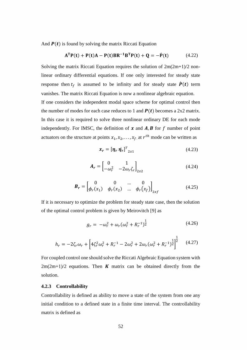
52

And 𝑷(𝒕) is found by solving the matrix Riccati Equation

𝐀𝐓𝐏(𝐭) + 𝐏(𝐭)𝐀 − 𝐏(𝐭)𝐁𝐑−𝟏𝐁𝐓𝐏(𝐭) + 𝐐 = −�̇�(𝐭) (4.22)

Solving the matrix Riccati Equation requires the solution of 2m(2m+1)/2 non-

linear ordinary differential equations. If one only interested for steady state

response then 𝑡𝑓 is assumed to be infinity and for steady state �̇�(𝒕) term

vanishes. The matrix Riccati Equation is now a nonlinear algebraic equation.

If one considers the independent modal space scheme for optimal control then

the number of modes for each case reduces to 1 and 𝑷(𝒕) becomes a 2x2 matrix.

In this case it is required to solve three nonlinear ordinary DE for each mode

independently. For IMSC, the definition of 𝒙 and 𝑨, 𝑩 for 𝑓 number of point

actuators on the structure at points 𝑥1, 𝑥2, . . . , 𝑥𝑓 . at 𝑟𝑡ℎ mode can be written as

𝒙𝒓 = [𝜼𝒓 𝜼�̇�]𝑇

2𝑥1 (4.23)

𝑨𝒓 = [0 1

−𝜔𝑟2 −2𝜔𝑟𝜁𝑟

]2𝑥2

(4.24)

𝑩𝒓 = [0 0 … 0

𝜙𝑟(𝑥1) 𝜙𝑟(𝑥2) … 𝜙𝑟(𝑥𝑓)]2𝑥𝑓

(4.25)

If it is necessary to optimize the problem for steady state case, then the solution

of the optimal control problem is given by Meirovitch [9] as

𝑔𝑟 = −𝜔𝑟2 + 𝜔𝑟(𝜔𝑟

2 + 𝑅𝑟−1)

12 (4.26)

ℎ𝑟 = −2𝜁𝑟𝜔𝑟 + [4𝜁𝑟2𝜔𝑟

2 + 𝑅𝑟−1 − 2𝜔𝑟

2 + 2𝜔𝑟(𝜔𝑟2 + 𝑅𝑟

−1)12]

12 (4.27)

For coupled control one should solve the Riccati Algebraic Equation system with

2m(2m+1)/2 equations. Then 𝑲 matrix can be obtained directly from the

solution.

4.2.3 Controllability

Controllability is defined as ability to move a state of the system from one any

initial condition to a defined state in a finite time interval. The controllability

matrix is defined as

53

𝑪 = [𝑩 𝑨𝑩 𝑨𝟐𝑩…𝑨𝟐𝒎−𝟏𝑩] (4.28)

And if the C matrix has the rank 2m then the system is deemed as controllable.

Figure 4-3 Uncontrollable and Controllable Systems [32]

Figure 4-3 shows uncontrollable and controllable system examples.

4.3 Observer Design

4.3.1 Introduction

Modal space control requires the modal displacement and velocity values to

calculate the necessary control input for the structure. However, it is not possible

to measure the modal coordinates physically. Therefore, either by using

displacement, velocity and acceleration measurements the modal states must be

estimated by using an observer.

Kalman has proposed an optimal observer that contains measurement and

actuator noise [36]. Luenberger has summed up observers for systems without

noise [37]. Luenberger observer is selected for the simulations in this study due

to its simplicity.

Placing the sensors to arbitrary nodes are not enough to find all the states. They

must be located such that observability matrix has full rank. Then, all the states

can be obtained and the selected control algorithm can be used.

4.3.2 Observability

Observability can be defined as the ability to obtain the every state of the plant

in finite time by using only the outputs of the system. The observability is based

on the rank of the matrix given below

54

𝑶 =

[

𝑪𝑪𝑨𝑪𝑨𝟐

…𝑪𝑨𝟐𝒎−𝟏]

(4.29)

If rank of 𝑶 equals to 2m, it is said that the plant is observable for our case.

4.3.3 Observer Design

The state space form of the plant is rewritten as

�̇� = 𝑨𝒙 + 𝑩𝒖 (4.30)

𝒚 = 𝑪𝒙 + 𝑫𝒖 (4.31)

Then an observer is designed to estimate the values of states and correcting itself

with the outputs taken from the exact system. The ~ mark is used to distinguish

observer from plant. 𝑲𝒆 is the observer feedback gain. The observer dynamics

can be written as

(�̃�)̇ = 𝑨𝒙 + 𝑩𝒖 + 𝑲𝒆[𝒚 − (𝑪�̃� + 𝑫𝒖)] (4.32)

(�̃�)̇ = 𝑨�̃� + 𝑩𝒖 + 𝑲𝒆𝒚 − 𝑲𝒆𝑪�̃� − 𝑲𝒆𝑫𝒖 (4.33)

Error is defined as the difference between the real states and estimated states

shown in the equation below

𝒆 = 𝒙 − (�̂�) (4.34)

Putting equation (4.31) into (4.33), and subtracting (4.33 from (4.30)

−[(�̃�)̇ = 𝑨�̃� + 𝑩𝒖 + 𝑲𝒆𝑪𝒙 + 𝑲𝒆𝑫𝒖 − 𝑲𝒆𝑪�̃� − 𝑲𝒆𝑫𝒖] (4.35)

+�̇� = 𝑨𝒙 + 𝑩𝒖 (4.36)

Will give the error rate between states.

�̇� − (�̃�)̇ = 𝑨(𝒙 − �̃�) − 𝑲𝒆𝑪(𝒙 − �̃�) (4.37)

�̇� = (𝑨 − 𝑲𝒆𝑪)𝒆 (4.38)

𝑲𝒆 is selected such that the poles of the observer are five to ten times larger than

the actual system. Observer model is shown in the figure below.

55

Figure 4-4 Observer and Plant [38]

4.4 Controlling Selected Modes

It is not always necessary to control all modelled modes of the structure. Then

one should modify the previous equations to control the selected modes of the

system. If 𝑚 is the total number of modelled modes, it can be divided as 𝑚𝑐 and

𝑚𝑟, number of controlled modes and number of residual modes respectively.

Also the states can be re-written as

𝑥 = [𝜼𝒄 �̇�𝒄 𝜼𝒓 �̇�𝒓]𝑇

where 𝜼𝒄 is the controlled mode vector and 𝜼𝒓 is the residual mode vector.

With the new states 𝑨 and 𝑩 matrices is required to be redefined. 𝑨 matrix is

separated into 𝑨𝒄 and 𝑨𝒓 matrices with the same structure of the original 𝑨

matrix. However they only contain their respective modes. It can be formulated

as

𝑨 = [𝑨𝒄 𝟎𝟎 𝑨𝒓

]

𝑩 = [𝑩𝒄

𝑩𝒓]

56

Where 𝑨𝒄 is 2mcx2mc and 𝑨𝒓 is 2mrx2mr sized matrix. 𝑩𝒄 matrix only contains

the mode shape values of controlled modes and 𝑩𝒓 contains the mode shape

values of residual modes.

One should also redefine the 𝑪 matrix to adapt the changed state vector.

𝐂 = [𝐂𝐜 𝐂𝐫]

Where 𝑪𝒄 is for controlled modes and 𝑪𝒓 for residual modes. 𝑫 matrix remains

unchanged.

The controller and estimator equations also require modification. Less number

of modes are controlled therefore less number of modes are necessary for

estimation. Now the controller defined in equation (4.1) is changed into

𝒖 = −𝑲𝒙𝒄

To find the controller gain 𝑲, same algorithms are used however instead of 𝑨 and

𝑩, 𝑨𝒄 and 𝑩𝒄 matrices are used. One can see that 𝒖 vector is multiplied by both

𝑩𝒄 and 𝑩𝒓. The controlled modes are contributing to the control of the system.

On the other hand residual modes are also contributing to the system response

and create unwanted oscillations. This is called control spillover. Meirovitch

stated that control spillover reduces the system performance but does not

destabilize the system.

Observer is modified such a way that only the modal states that are needed for

the controlled modes are estimated. Residual modes are not estimated therefore

their effect cannot be put into the observer equation. Then equations (4.32) can

be written as

�̇̃�𝒄 = 𝑨𝑪�̃�𝒄 + 𝑩𝒄𝒖 + 𝑲𝒆[𝒚 − (𝑪𝒄�̃�𝒄 + 𝑫𝒖)] (4.39)

However in the real case the output is sum of both controlled modes and residual

modes. Modes that are not contributed into the observer create an error and it is

called observation spillover. Meirovitch stated that observation spillover can

destabilize the system. To overcome the problem it is stated that active vibration

control is mostly used on lower modes and upper modes are selected as residual

modes. One can filter out the higher frequencies to prevent observer spillover.

57

CHAPTER 5

CASE STUDIES

5.1 Introduction

In this chapter case studies will be demonstrated. Two models will be used;

simply supported beam with transverse vibrations and a three dimensional

complex shape shown in Chapter 3 with three translational degrees of freedom

at each node.

Number of controlled modes, location of sensors, actuators and disturbances are

changed to show the applicability of control algorithms. For applicable

conditions independent modal space control and coupled control is shown. For

other cases only coupled control is used.

Matlab and Simulink are used to simulate the models. Response of the each

controller and controller force is compared with each other. For optimal control

different R (weight of the actuator) is used.

5.2 Simply Supported Beam

5.2.1 Model Definition

A simply supported beam shown in Chapter 3 is used in the case study. Its

properties are shown in Table 5.1

Table 5-1 Simply Supported Beam Properties

Length 1000 mm

Width 100 mm

Height 10 mm

Young’s Modulus of Elasticity 70 Gpa

Density 2700 kg/m3

Boundary Conditions Pinned from both ends

Number of Nodes 21

Number of modelled Modes 6

It was shown that the results of the finite element model results are in good

agreement the analytical case. Actually, error of natural frequencies and mode

shapes are less than 1% for the first six modes. First six natural frequencies are

shown in Table 5.2.

58

Table 5-2 Simply Supported Beam Natural Frequencies

1st Mode 2nd Mode 3rd Mode 4th Mode 5th Mode 6th Mode

23.086 Hz 92.306 Hz 207.550

Hz

368.600

Hz

575.120

Hz

826.570

Hz

The mode shape matrix is given in Table 5.3. It is necessary to display it here to

show how to locate the sensors and actuators. The numbering of nodes are shown

in Figure 5.1.

Table 5-3 Mode Shapes Matrix of the Simply Supported Beam

Node 1st Mode 2nd Mode 3rd Mode 4th Mode 5th Mode 6th Mode

1 0 0 0 0 0 0

2 -0.134637 0.265959 -0.39073 -0.50589 0.608581 0.696291

3 -0.265959 0.505885 -0.69629 -0.81854 0.860663 0.818539

4 -0.390733 0.696291 -0.85007 -0.81854 0.608581 0.265959

5 -0.505885 0.818539 -0.81854 -0.50589 0 -0.50589

6 -0.608581 0.860663 -0.60858 0 -0.60858 -0.86066

7 -0.696291 0.818539 -0.26596 0.505885 -0.86066 -0.50589

8 -0.766856 0.696291 0.134637 0.818539 -0.60858 0.265959

9 -0.818539 0.505885 0.505885 0.818539 0 0.818539

10 -0.850067 0.26596 0.766856 0.505885 0.608581 0.696291

11 -0.860663 0 0.860663 0 0.860663 0

12 -0.850067 -0.26596 0.766856 -0.50589 0.608581 -0.69629

13 -0.818539 -0.50589 0.505885 -0.81854 0 -0.81854

14 -0.766856 -0.69629 0.134638 -0.81854 -0.60858 -0.26596

15 -0.696291 -0.81854 -0.26596 -0.50589 -0.86066 0.505885

16 -0.608581 -0.86066 -0.60858 0 -0.60858 0.860663

17 -0.505885 -0.81854 -0.81854 0.505885 0 0.505885

18 -0.390733 -0.69629 -0.85007 0.818539 0.608581 -0.26596

19 -0.26596 -0.50589 -0.69629 0.818539 0.860663 -0.81854

20 -0.134637 -0.26596 -0.39073 0.505885 0.608581 -0.69629

21 0 0 0 0 0 0

Figure 5-1 Node Numbers of Simply Supported Beam

Beam is vibrating in the Y direction and pinned at the nodes 1 and 21.

59

5.2.2 Case Studies

5.2.2.1 First Mode Control

In this case study only first mode will be controlled with one sensor and one

actuator and one disturbance force. Step input and a sinusoidal input will be

given to the system. Force response function will be obtained for selected cases.

1% damping is introduced into the model for each mode. As the number of

actuator is equal to the number of controlled mode, independent modal space

control is applicable in this case. The aim is to re-locate the damping of first

mode to 1/√2.

For the first sub-case, disturbance will be put at 6th node with 1 Newton

amplitude, displacement sensor at 10th node and actuator at 11th node. Also R

is taken as 0.001. Then for step input the results are shown in the figure 5.2. The

required force for each case is given in the figures 5.3

Figure 5-2 Simply Supported Beam Response to Step Input

0.1 0.2 0.3 0.4 0.5

0

0.005

0.01

0.015

0.02

0.025

0.03

0.035

0.04

0.045

time(seconds)

dis

pla

cem

ent(

mm

)

SSB Step Input Response

Open Loop

Coupled Pole Placement

Coupled Optimal Control

Independent Pole Placement

Independent Optimal Control

60

Figure 5-3 Simply Supported Beam Force Comparison to Step Response

Disturbance

The response to step input is satisfactory such that vibrations are reduced in less

than 0.05 seconds for pole placement case. For optimal control different R

values are compared in the Figure 5.4. In the figure 5.5 force required to control

the system is shown. To compare them easily, their absolute value is taken. One

can select an appropriate R value for the available maximum force output of the

actuator.

0 0.1 0.2 0.3 0.4 0.5 0.6 0.7 0.8-0.6

-0.5

-0.4

-0.3

-0.2

-0.1

0

0.1

0.2

time(seconds)

Forc

e(N

)

Coupled Pole Placement

Coupled Optimal Control

Independent Pole Placement

Independent Optimal Control

61

Figure 5-4 SSB Step Response Coupled Optimal Control for Different R

values (displacement)

Figure 5-5 SSB Step Response Coupled Optimal Control for Different R

values (Force)

0 0.2 0.4 0.6 0.8 1 1.2

0.005

0.01

0.015

0.02

0.025

0.03

0.035

0.04

0.045

0.05

time(seconds)

dis

pla

cem

ent(

mm

)

SSB Coupled Optimal Control R value Effect

Open Loop

R=1e-2

R=1e-3

R=1e-4

R=1e-5

0 0.1 0.2 0.3 0.4 0.5

-0.6

-0.4

-0.2

0

0.2

0.4

0.6

time(seconds)

Forc

e(N

)

SSB Coupled Optimal Control R value Effect

R=1e-2

R=1e-3

R=1e-4

R=1e-5

62

Figure 5-6 SSB Step Response Independent Optimal Control for Different

R values (displacement)

Figure 5-7 SSB Step Response Independent Optimal Control for Different

R values (displacement)

0 0.2 0.4 0.6 0.8

0

0.005

0.01

0.015

0.02

0.025

0.03

0.035

0.04

0.045

0.05

time(seconds)

dis

pla

cem

ent(

mm

)SSB Independent Optimal Control R value Effect

Open Loop

R=1e-2

R=1e-3

R=1e-4

R=1e-5

0 0.1 0.2 0.3 0.4 0.5

-0.6

-0.4

-0.2

0

0.2

0.4

0.6

time(seconds)

Forc

e(N

)

SSB Independent Optimal Control R value Effect

R=1e-2

R=1e-3

R=1e-4

R=1e-5

63

It is seen that as R increases the required force decreases, however in the same

time the oscillations continue longer.

Now the response of the system to sinusoidal input will be shown. A chirp signal

from 2 Hz to 100 Hz is given in 100 seconds. In Simulink ode8 is used as fixed

time step solver. Time step is given as 1/10000 seconds. Then Fast Fourier

Transform(FFT) is made in Matlab. The Matlab Code for FFT is given in

Appendix A The results are shown in figure 5.8.

It is seen that there is more than 20 dB decrease at the first mode for optimal

control(R=0.001) and more than 30 dB decrease for pole placement. As we only

control the first mode there is no change at the second mode response at the

frequency around 92 Hz.

Figure 5-8 Simply Supported Beam, Frequency Response Function

between 0-100 Hz, One Mode Control

5.2.2.2 First and Second Mode Control

In the previous sub-case it is shown that first mode is controlled. If it is necessary

to control the second mode also, we need to increase the number of controlled

modes to 2. In the simulation it is seen that another sensor is necessary to obtain

convergence. It is probably due to observation spillover. Then the sensor

10 20 30 40 50 60 70 80 90 100-120

-110

-100

-90

-80

-70

-60

-50

-40

-30

Frequency (Hz)

dB

SSB FRF to Chirp Signal 2-100Hz

Open Loop

Coupled Pole Placement

Coupled Optimal Control

Independent Pole Placement

Indepedendent Optimal Control

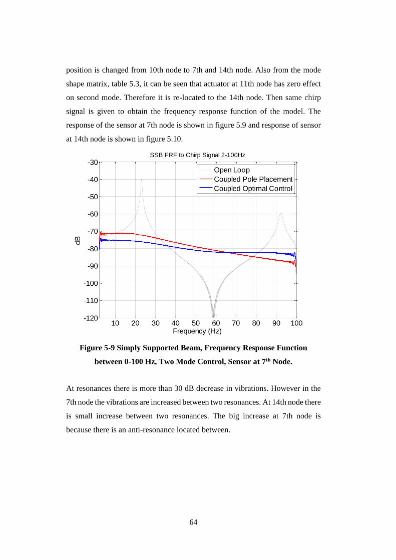
64

position is changed from 10th node to 7th and 14th node. Also from the mode

shape matrix, table 5.3, it can be seen that actuator at 11th node has zero effect

on second mode. Therefore it is re-located to the 14th node. Then same chirp

signal is given to obtain the frequency response function of the model. The

response of the sensor at 7th node is shown in figure 5.9 and response of sensor

at 14th node is shown in figure 5.10.

Figure 5-9 Simply Supported Beam, Frequency Response Function

between 0-100 Hz, Two Mode Control, Sensor at 7th Node.

At resonances there is more than 30 dB decrease in vibrations. However in the

7th node the vibrations are increased between two resonances. At 14th node there

is small increase between two resonances. The big increase at 7th node is

because there is an anti-resonance located between.

10 20 30 40 50 60 70 80 90 100-120

-110

-100

-90

-80

-70

-60

-50

-40

-30

Frequency (Hz)

dB

SSB FRF to Chirp Signal 2-100Hz

Open Loop

Coupled Pole Placement

Coupled Optimal Control

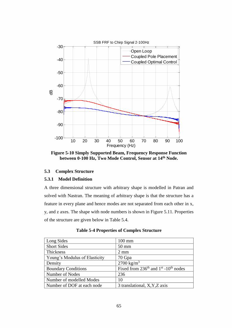
65

Figure 5-10 Simply Supported Beam, Frequency Response Function

between 0-100 Hz, Two Mode Control, Sensor at 14th Node.

5.3 Complex Structure

5.3.1 Model Definition

A three dimensional structure with arbitrary shape is modelled in Patran and

solved with Nastran. The meaning of arbitrary shape is that the structure has a

feature in every plane and hence modes are not separated from each other in x,

y, and z axes. The shape with node numbers is shown in Figure 5.11. Properties

of the structure are given below in Table 5.4.

Table 5-4 Properties of Complex Structure

Long Sides 100 mm

Short Sides 50 mm

Thickness 2 mm

Young’s Modulus of Elasticity 70 Gpa

Density 2700 kg/m3

Boundary Conditions Fixed from 236th and 1st -10th nodes

Number of Nodes 236

Number of modelled Modes 10

Number of DOF at each node 3 translational, X,Y,Z axis

10 20 30 40 50 60 70 80 90 100-100

-90

-80

-70

-60

-50

-40

-30

Frequency (Hz)

dB

SSB FRF to Chirp Signal 2-100Hz

Open Loop

Coupled Pole Placement

Coupled Optimal Control

66

Figure 5-11 Complex Structure with Finite Element Node Numbers

It is modelled with 10 modes, 236 nodes and three translational degrees of

freedom at each node. The 10 mode shapes and natural frequencies are shown in

Table 5.5.

Table 5-5 Complex Structure First Ten Mode Shapes and Natural

Frequencies

67

5.3.2 Case Studies

At first, 1st mode shape will be controlled. Secondly 1st and 2nd mode shapes

will be controlled. In the third case only 5th mode shape will be controlled to

show that higher local modes can be controlled with modal control approach.

5.3.2.1 First Mode Control

From Table 5.5 it can be seen that at first mode the structure is vibrating in ZY

plane (around X axis). It is seen that there is displacement in both Y direction

and Z direction. Therefore sensor and actuator can be put in those directions. A

disturbance will be put such that it has a significant effect on 1st mode. For

different locations and directions of sensor, actuator and disturbance, the

resultant open loop and closed loop responses are shown.

i) From table 5.5 it can be seen that most displacement on first mode is at the

node 235. Then sensor and actuator is co-placed at that point. Disturbance is

68

given at the node 130, which also have an effect on first mode. Ode23t solver

with 0.5 simulation time is used. R value for optimal control is taken as 0.001.

The results are shown in the figure 5.12.

Sensor Location -

Axis

Actuator Location -

Axis

Disturbance Location -

Axis

235th node Z axis 235th node Z axis 130th node Z axis

Figure 5-12 Complex Structure response to Step Input. Sensor Z axis,

Actuator Z axis, Co-placed.

ii) In this case sensor direction is changed from Z axis to Y axis. The actuator

and sensor are still co-placed. The result is shown in the figure 5.13

Sensor Location -

Axis

Actuator Location -

Axis

Disturbance Location -

Axis

235th node Y axis 235th node Z axis 130th node Z axis

0 0.1 0.2 0.3 0.4 0.50

0.05

0.1

0.15

0.2

0.25

time(seconds)

dis

pla

cem

ent(

mm

)

Step Response of 3D Structure

Open Loop

Coupled Pole Placement

Coupled Optimal Control

Independent Pole Placement

Independent Optimal Control

69

Figure 5-13 Complex Structure response to Step Input. Sensor Y axis,

Actuator Z axis, Co-placed

iii) Sensor is relocated such that it is now sensing the Z axis displacement from

the node 170. The results are shown in the Figure 5.14

Sensor Location -

Axis

Actuator Location -

Axis

Disturbance Location -

Axis

170th node Z axis 235th node Z axis 130th node Z axis

0 0.05 0.1 0.15 0.2

-0.2

-0.15

-0.1

-0.05

0

time(seconds)

dis

pla

cem

ent(

mm

)

Step Response of 3D Structure

Open Loop

Coupled Pole Placement

Coupled Optimal Control

Independent Pole Placement

Independent Optimal Control

70

Figure 5-14 Complex Structure response to Step Input. Sensor Z axis,

Actuator Z axis, Not Co-placed

iv) In the fourth case the sensor is placed such that it is not co-placed and senses

the displacement in Y axis. The results are shown in Figure 5.15.

Sensor Location -

Axis

Actuator Location -

Axis

Disturbance Location -

Axis

170th node Y axis 235th node Z axis 130th node Z axis

0 0.1 0.2 0.3 0.4 0.50

0.02

0.04

0.06

0.08

0.1

0.12

0.14

time(seconds)

dis

pla

cem

ent(

mm

)Step Response of 3D Structure

Open Loop

Coupled Pole Placement

Coupled Optimal Control

Independent Pole Placement

Independent Optimal Control

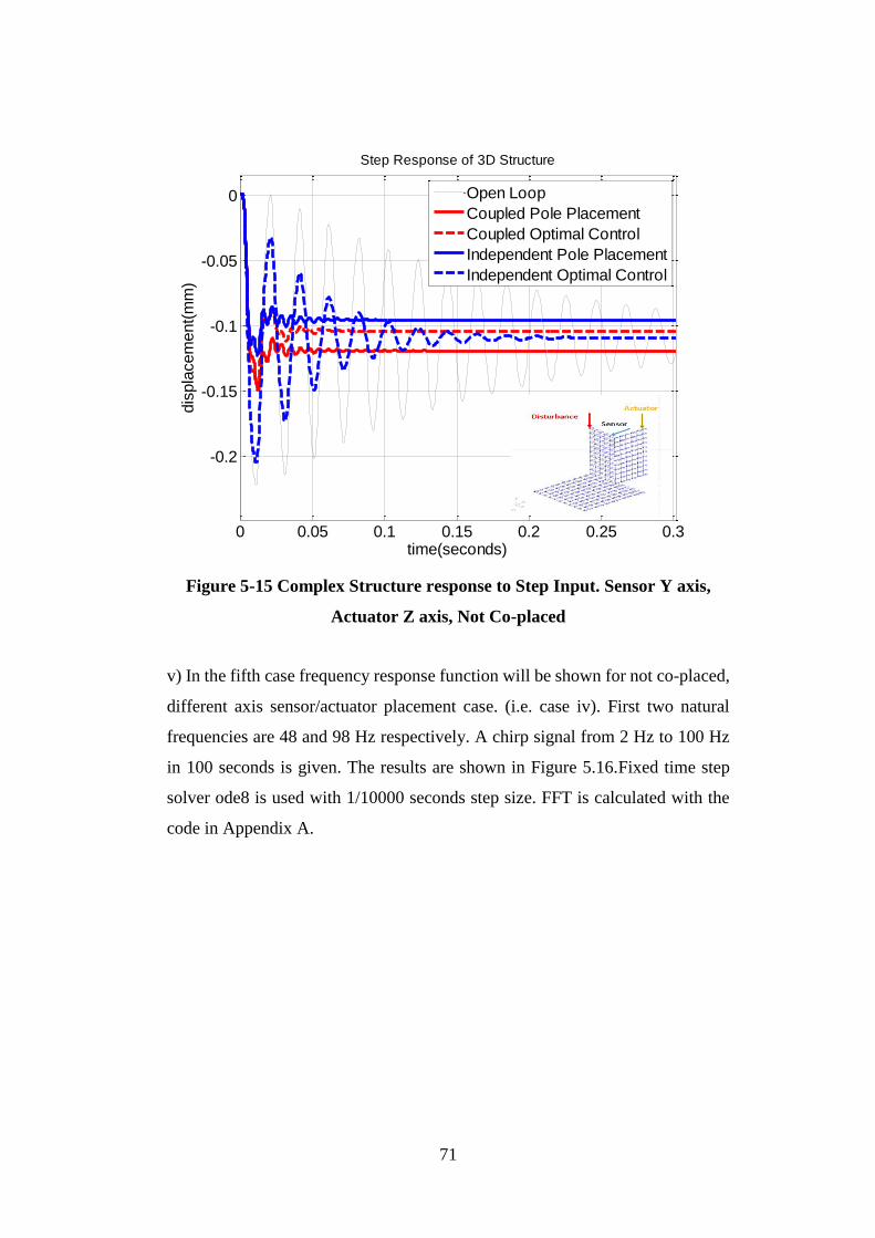
71

Figure 5-15 Complex Structure response to Step Input. Sensor Y axis,

Actuator Z axis, Not Co-placed

v) In the fifth case frequency response function will be shown for not co-placed,

different axis sensor/actuator placement case. (i.e. case iv). First two natural

frequencies are 48 and 98 Hz respectively. A chirp signal from 2 Hz to 100 Hz

in 100 seconds is given. The results are shown in Figure 5.16.Fixed time step

solver ode8 is used with 1/10000 seconds step size. FFT is calculated with the

code in Appendix A.

0 0.05 0.1 0.15 0.2 0.25 0.3

-0.2

-0.15

-0.1

-0.05

0

time(seconds)

dis

pla

cem

ent(

mm

)

Step Response of 3D Structure

Open Loop

Coupled Pole Placement

Coupled Optimal Control

Independent Pole Placement

Independent Optimal Control

72

Figure 5-16 Complex Structure response to Chirp Signal from 2 Hz to 100

Hz. Sensor Y axis, Actuator Z axis, Not Co-placed

5.3.2.2 First and Second Mode Control

To control the second mode, in addition to a sensor at Y or Z axis, another sensor

for X axis is necessary. Similarly another actuator is necessary to control the

vibrations in X axis. Then with two actuators and two sensors the complex

structure will be controlled.

i) Co-placed actuator and sensor pair will be put at 235th node at X and Y axis.

A disturbance will be given from the 130th node at X,Y,Z directions. The result

of two sensors are shown in Figure 5.17 and 5.18

Sensor Location - Axis Actuator Location -

Axis

Disturbance Location -

Axis

235th node X axis 235th node X axis 130th node X axis

235th node Y axis 235th node Y axis 130th node Y axis

- - 130th node Z axis

10 20 30 40 50 60 70 80 90-70

-60

-50

-40

-30

-20

-10

Frequency (Hz)

dB

3D Model FRF to Chirp Signal 2-100Hz

Open Loop

Coupled Pole Placement

Coupled Optimal Control

Independent Pole Placement

Indepedendent Optimal Control

73

Figure 5-17 Complex Structure, response to step input X axis results.

Figure 5-18 Complex Structure, response to step input Y axis results

0 0.05 0.1 0.15 0.2-0.2

0

0.2

0.4

0.6

0.8

1

1.2

1.4

1.6

time(seconds)

dis

pla

cem

ent(

mm

)

Step Response of 3D Structure

Open Loop

Coupled Pole Placement

Coupled Optimal Control

Independent Pole Placement

Independent Optimal Control

0 0.05 0.1 0.15 0.2-0.2

0

0.2

0.4

0.6

0.8

1

1.2

1.4

1.6

time(seconds)

dis

pla

cem

ent(

mm

)

Step Response of 3D Structure

Open Loop

Coupled Pole Placement

Coupled Optimal Control

Independent Pole Placement

Independent Optimal Control

74

ii) In the second case a non co-placed sensor actuator pair will be used. The

results are shown in the Figure 5.19 and 5.20

Sensor Location - Axis Actuator Location -

Axis

Disturbance Location -

Axis

208th node X axis 235th node X axis 130th node X axis

208th node Y axis 235th node Y axis 130th node Y axis

- - 130th node Z axis

Figure 5-19 Complex Structure, response to step input X axis results. Non

Co-placed sensor and actuator

0 0.05 0.1 0.15 0.2-0.1

0

0.1

0.2

0.3

0.4

0.5

0.6

time(seconds)

dis

pla

cem

ent(

mm

)

Step Response of 3D Structure

Open Loop

Coupled Pole Placement

Coupled Optimal Control

Independent Pole Placement

Independent Optimal Control

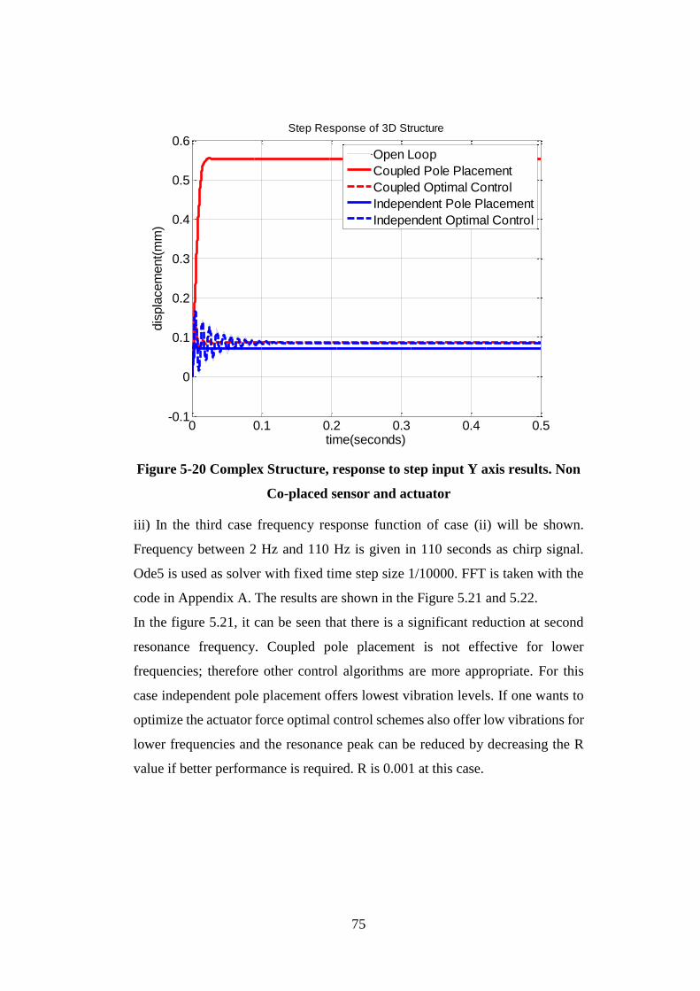
75

Figure 5-20 Complex Structure, response to step input Y axis results. Non

Co-placed sensor and actuator

iii) In the third case frequency response function of case (ii) will be shown.

Frequency between 2 Hz and 110 Hz is given in 110 seconds as chirp signal.

Ode5 is used as solver with fixed time step size 1/10000. FFT is taken with the

code in Appendix A. The results are shown in the Figure 5.21 and 5.22.

In the figure 5.21, it can be seen that there is a significant reduction at second

resonance frequency. Coupled pole placement is not effective for lower

frequencies; therefore other control algorithms are more appropriate. For this

case independent pole placement offers lowest vibration levels. If one wants to

optimize the actuator force optimal control schemes also offer low vibrations for

lower frequencies and the resonance peak can be reduced by decreasing the R

value if better performance is required. R is 0.001 at this case.

0 0.1 0.2 0.3 0.4 0.5-0.1

0

0.1

0.2

0.3

0.4

0.5

0.6

time(seconds)

dis

pla

cem

ent(

mm

)

Step Response of 3D Structure

Open Loop

Coupled Pole Placement

Coupled Optimal Control

Independent Pole Placement

Independent Optimal Control

76

Figure 5-21 Complex Structure, X axis sensor frequency response

function. Non Co-placed sensor and actuator

From figure 5.22 Y axis results can be read. First mode is dominant for Y axis

and with the control algorithms the vibrations can be reduced more than 20 dB

at resonance. Coupled pole placement increases the vibrations at lower

frequencies, therefore other control algorithms may be chosen. However for

higher frequencies coupled control is better.

20 40 60 80 100 120-100

-90

-80

-70

-60

-50

-40

-30

Frequency (Hz)

dB

3D Model FRF to Chirp Signal 2-110Hz

Open Loop

Coupled Pole Placement

Coupled Optimal Control

Independent Pole Placement

Indepedendent Optimal Control

77

Figure 5-22 Complex Structure, Y axis sensor frequency response

function. Non Co-placed sensor and actuator

5.3.2.3 Local Mode Control (5th Mode)

In this case study only a higher mode will be controlled assuming that it is

excited by an external disturbance. Indeed its natural frequency is high(around

620 Hz) this case will demonstrate the applicability of modal space control to

control local modes of a structure.

From Figure 5.11 and Table 5.5 it can be seen that node 120 is most affected by

5th mode vibrations. Then we place the disturbance to this node at Z axis.

Assume that we cannot put the sensor and actuator in the same location (not co-

placed) and also they cannot put on the disturbance. Actuator location is selected

to be 96th node and sensor location is selected to be 108th node. Indeed they

have to be located nearly as it is a local mode and it does not affect other sides

of the structure.

20 40 60 80 100 120-100

-90

-80

-70

-60

-50

-40

-30

Frequency (Hz)

dB

3D Model FRF to Chirp Signal 2-110Hz

Open Loop

Coupled Pole Placement

Coupled Optimal Control

Independent Pole Placement

Indepedendent Optimal Control

78

Sensor Location -

Axis

Actuator Location -

Axis

Disturbance Location -

Axis

108th node Z axis 96th node Z axis 120th node Z axis

The damping is tried to be located at 1/√2. However coupled control cannot

converge therefore the necessary damping ratio is reduced to 1/2. (i.e from 0.707

to 0.5). Then the result is shown in the Figure 5.23. For optimal control

parameter R is taken as 0.0001

Figure 5-23 Local Mode Control Results to Step Input

An FRF analysis is done between 30 Hz and 900 Hz and results are given in the

figure 5.24. It can be seen that there is a reduction around 620 Hz. Also there is

reduction at 1st, 2nd and 3rd mode. But there is no reduction at 4th mode. From

table 5.5 it can be seen that first three modes also has a Z direction displacement

at that local area, but 4th mode does not have that displacement. Indeed it is only

wanted to control the 5th mode, first three modes vibration is also reduced. This

explains the good step input response of the system as it is not expected to have

a good step response by only controlling 5th mode as its contribution is greatly

lower than first four mode.

0 0.1 0.2 0.3 0.4 0.50

0.05

0.1

0.15

0.2

0.25

time(seconds)

dis

pla

cem

ent(

mm

)

Step Response of 3D Structure

Open Loop

Coupled Pole Placement

Coupled Optimal Control

Independent Pole Placement

Independent Optimal Control

79

Figure 5-24 Frequency Response Function of Local Mode Control to A

Chirp Excitation

Figure 5-25 Frequency Response Function of Local Mode Control to A

Chirp Excitation Close Up View First and Second Mode

100 200 300 400 500 600 700 800 900-130

-120

-110

-100

-90

-80

-70

-60

-50

-40

-30

Frequency (Hz)

dB

3D Model FRF to Chirp Signal 30-900 Hz

Open Loop

Coupled Pole Placement

Coupled Optimal Control

Independent Pole Placement

Indepedendent Optimal Control

40 60 80 100 120

-110

-100

-90

-80

-70

-60

-50

-40

Frequency (Hz)

dB

3D Model FRF to Chirp Signal 30-900 Hz

Open Loop

Coupled Pole Placement

Coupled Optimal Control

Independent Pole Placement

Indepedendent Optimal Control

80

Figure 5-26 Frequency Response Function of Local Mode Control to A

Chirp Excitation Close Up View Third Mode

Figure 5-27 Frequency Response Function of Local Mode Control to A

Chirp Excitation Close Up View Fifth Mode

130 140 150 160 170 180 190 200

-110

-105

-100

-95

-90

-85

-80

-75

-70

-65

Frequency (Hz)

dB

3D Model FRF to Chirp Signal 30-900 Hz

Open Loop

Coupled Pole Placement

Coupled Optimal Control

Independent Pole Placement

Indepedendent Optimal Control

130 140 150 160 170 180 190 200

-110

-105

-100

-95

-90

-85

-80

-75

-70

-65

Frequency (Hz)

dB

3D Model FRF to Chirp Signal 30-900 Hz

Open Loop

Coupled Pole Placement

Coupled Optimal Control

Independent Pole Placement

Indepedendent Optimal Control

81

CHAPTER 6

CONCLUSION

6.1 Discussion

Modal space feedback control is effective at reducing vibrations at resonances.

However at other than resonance frequencies, vibrations may be amplified. By

selecting proper controller this problem can be solved. If the structure is excited

with forced vibrations at frequencies other than resonance frequencies one can

also implement feed forward controller to improve the efficiency.

In this study displacement sensors are used to observe the system. Velocity

sensors are similar to displacement sensors. However when an accelerometer

sensor is introduced, D matrix is no longer a null matrix. Then observation

spillover can destabilize the system easier. To prevent this problem one should

use more sensors until stability is achieved.

To get the maximum efficiency from the actuator one should place the

actuator(s) at the point that the mode shape value of the controlled mode(s)

is(are) maximum. To reduce the control spillover, one should choose a location

such that the mode shape value of uncontrolled modes are minimum. Same

approach should be used for sensor placement. It will reduce observation

spillover and provide better observer performance.

A proposed experimental setup can be composed of a simply supported

beam/cantilever beam, accelerometer sensors and force generator(s). Force

generator can be an electric motor with unbalance mass. The phase and speed of

the unbalance mass must be controllable. To prevent vibrations in other

directions then controlled direction, one can use a 2nd actuator that counter

balances the 1st actuator. Finite element modal can be modelled with lumped

masses of sensors and actuators. Also one can make an impact test to obtain FRF

between actuator(s) and sensor(s). To disturb the structure a hammer can be used

82

for impulse input. For sinusoidal excitation a shaker table or directly a shaker

can be used. Moreover an extra motor pair can be added to disturb the structure.

6.2 Conclusion

Literature review on active vibration control focused on modal domain reveals

that most of the studies are limited to simple structures such as beams and plates.

Therefore, it is aimed to study the application of modal domain control on more

complex arbitrary shaped structures with the help of finite element analysis tools.

The methodology is developed first considering vibrations of a one dimensional

structure (simply supported beam) which is modelled as distributed model with

partial differential equations. Then, the orthogonality property is shown and

stated that each mode is independent from each other. It is also shown that the

displacement, velocity or acceleration of a structure can be written as infinite

sum of its modes. Finally, the independent equations in modal domain are

written in state space form. They are simulated with Simulink and the results are

compared with the analytical response. The response to sinusoidal input is

compared with analytical formulation and the model is verified.

Later, discretization of a one dimensional structure is demonstrated. Then, the

generalization of a three dimensional model formulation is studied. Discretized

one dimensional model is compared with continuous model. Both are simulated

in Simulink and the results are verified. Finally, a three dimensional complex

shaped structure is used to show the generalized formulation.

Control studies start with the feedback control algorithms that are implemented

in state space. Four algorithms are investigated, coupled pole placement, coupled

optimal control, independent pole placement and independent optimal control.

Controllability and observability are investigated. Finally, an observer to

estimate the states of the state space model is introduced.

Case studies are presented to show the application of modal domain control.

First, simply supported beam vibrations are controlled and it is shown that

different number of modes can be controlled. Second, the three dimensional

complex shaped structures vibrations are controlled. Co-located and non co-

located control strategies are tried. Also co-oriented and non co-oriented sensor

83

and actuator placements are tried. It is shown that as long as states are correctly

estimated sensor and actuator does not have to be co-oriented. (i.e. sensor is

sensing displacement in X axis, actuator is acting force on Y axis). Furthermore,

local mode vibrations of the structure are controlled. For different cases

frequency response functions are obtained to show the general performance of

the control forces.

6.3 Future Work

In this study it is assumed that there is no actuator or measurement noise.

Therefore, a Luenberger observer was sufficient to estimate the states. For noisy

actuator and sensors a Kalman Filter can be used.

Instead of using point forces on nodes, piezoelectric actuators can be

implemented into the model as they are widely used in the active vibration

control applications.

Observer spillover is a significant problem that alters the stability of the system.

To overcome this problem a low-pass or band-pass filter can be used to filter out

the residual modes.

Optimal placement of sensor and actuators are not studied in this work. However

with optimal placement, number of actuators/sensors and peak force required

can be reduced and stability margin of the system can be increased.

84

85

REFERENCES

[1] Nagaraj V.T., “3rd Short Course on Helicopter Design Notes”, Konkuk

Univesity, 2010

[2] Chopra I., Datta A., “Helicopter Dynamics”, ENAE 633 Course Book,

University of Maryland, 2011

[3] Tan A.C.H., Meurers T., Veres S.M., Aglietti G., Rogers E.,“Satellite

Vibration Control Using Frequency Selective Feedback”, Proceedings of the 42nd

IEEE Conference on Decision and Control Maui, Hawaii USA,December, 2013

[4] Irvine T., “ISS Solar Panel Vibration”, www.vibrationdata.com, 2010

[5] Torbati M.M., Keane A.J., Elliott S.J., Brennan M.J., Anthony D.K., Rogers

E.,“Active vibration control (AVC) of a satellite boom structure using optimally

positioned stacked piezoelectric actuators”, Journal of Sound and Vibration

vol.292, 203-220, 2006

[6] Zhi-Le W., Bo L., Yuan Z., Hao-Su X., Cheng-Hao Z.,“Satellite Vibration

on Image Quality Degradation of Remote Sensing Camera”, Research on

Precision Instrument and Machinery(RPIM), vol.1, issue 1., 2012

[7] Irvine T., “Vibration In Rocket Vehicles Due To Combustion Instability

Revision F”, www.vibrationdata.com, 2011

[8] Irvine T., “Solid Rocket Motor Pressure Oscillation Frequencies Revision

A”, www.vibrationdata.com, 2011

[9] L. Meirovitch (1989), Dynamics and Control of Structures, Virginia, John

Wiley & Sons

[10] Balas M.J., Active Control of Flexible Systems, Journal of Optimization

Theory and Applications, Vol:25 No:3, 1978

[11] Meirovitch L., Öz H., “Modal-Space Control of Large Flexible Spacecraft

Possessing Ignorable Coordinates”, Journal of Guidance and Control, vol.3, no.

6, Nov.-Dec.,1980

[12] Meirovitch, L., & Baruht, H., Optimal Control of Damped Flexible

Gyroscopic Systems. Journal of Guidance and Control, 4(2), 157-163, 1981

[13] Vasques, C., & Rodrigues, J. D., Active vibration control of smart

piezoelectric beams: Comparison of classical and optimal feedback control

strategies. Computers and Structures No:84, 1402-1414, 2006

[14] - Meirovitch, L., & Baruht, H, Control of Self-Adjoint Distributed-

Parameter Systems, Journal of Guidance, Vol:5 No:1, 60-66, 1981

[15] Resta F., Ripamonti F.,.Cazzulani G, Ferrari M., Independent modal control

for nonlinear flexible structures:An experimental test rig, Journal of Sound and

Vibration 329, 961-972, 2010

86

[16] Lindberg Jr. R.E., Longman R.W., “On the Number and Placement of

Actuators for Independent Modal Space Control”, Journal of Guidance and

Control, vol.7, no.2, March-April, 1984

[17] Qiu Z., Zhang X., Wu H., Zhang H., Optimal placement and active vibration

control for piezoelectric smart flexible cantilever plate, Journal of Sound and

Vibration 301, 521-543, 2007

[18] Jemai B., Ichchou M.N., Jezequel L., An Assembled Plate Active Control

Damping Set-Up: Optimization and Control, Journal of Vibraton and Control

225, 327-343, 1999

[19] Xu B., Jiang J. S., Integrated optimization of structure and control for

piezoelectric intelligent trusses with uncertain placement of actuators and

sensors, Computational Mechanics 33, 406-412 , 2004

[20] Canfield R., Meirovitch L., Integrated Structural Design and Vibration

Suppression Using Independent Modal Space Control, AIAA Journal, Vol 32,

No: 10, 1994

[21] Meirovitch L.,Baruh H., Oz H., A Comparison of Control Techniques for

Large Flexible Systems, Journal of Guidance , Vol:6, No:4, 302-310, 1983

[22] Meirovitch L., Baruh H., “Robustness of the Independent Modal-Space

Control Method”, Journal of Guidance, vol.6, no.1, Jan-Feb, 1983

[23] Baz, A., Poh S., Studer P., “Modified independent modal space control

method for active control of flexible systems”, Proceedings of the Institution of

Mechanical Engineers, Part C: Journal of Mechanical Engineering Science,

vol.203, no. 2, 103-112, 1988

[24] Singh S.P., Pruthi H.S., Agarwal V.P., Efficient modal control strategies for

active control of vibrations, Journal of Sound and Vibration 262, 563-575, 2003

[25] Öz, H., “Independent modal-space control and estimation with distributed

piezoelectric actuators and sensors”, Proc. SPIE 2715, Smart Structures and

Materials 1996: Mathematics and Control in Smart Sturcutres, 196,1996.

[26] Fang J.Q., Li Q.S., Jeary A.P., “Modified independent modal space control

of m.d.o.f. systems”, Journal of Sound and Vibration, vol.261, issue 3, 421-441,

2003

[27] Lin Y.H., Yu H.C., “Active modal control of a flexible rotor”, Journal of

Mechanical System and Signal Processing, vol.18, 1117-1131, 2004

[28] Poh S., Baz.A, “Active Control of a Flexible Structure Using a Modal

Positive Position Feedback Controller”, NASA Technical Report, 1990

[29] Hurlebaus S., Stöbener U., Gaul L., “Vibration reduction of curved panels

by active modal control”, Journal of Computers and Structures, vol.86, 251-257,

2008

87

[30] Serra, M., Resta F., Ripamonti F., “Dependent Modal Space

Control”,Journal of Smart Materials and Structures, vol.22, no.10, 2013

[31] L. Meirovitch (2001), Fundamentals of Vibrations, Virginia, McGraw Hill

[32] Inman D.J.(2006), “Vibration with Control”, Virginia USA, John Wiley &

Sons

[33] R. Pathi , Pole Placement Control Design, http://nptel.ac.in/, last visited

November 2014

[34] Budynas R.G & Nisbett J.K (2011), Shigley’s Mechanical Engineering

Design 9th Edition, USA, McGraw Hill

[35] System Dynamics - The Effect of Pole Location on Response,

http://www.facstaff.bucknell.edu/mastascu/econtrolhtml/SysDyn/SysDyn2Pole

Location.html, last visited November 2014

[36] Kalman R.E., A New Approach to Linear Filtering and Prediction

Problems, ASME Transactions, Vol. 82 Part D pp. 35-45, Journal of Basic

Engineering, 1960

[37] Luenberger D.G. , An Introduction to Observers, IEEE Transactions on

Automatic Control, Vol. AC-16, No:6, December 1971

[38] Fuller C.R, Elliott S. J., Nelson P.A (1997), Active Control of Vibration,

USA, Elsevier

[39] Silva L.A., Inman D.J., “On the Application of Independent Modal-Space

Control to Internal Variable Based Viscoelastic Bar”, Proceedings of SPIE - The

International Society for Optical Engineering, vol.4753, no. I, 247-252, 2002

[40] Meirovitch L., Öz H., “Stochastic Independent Modal-Space Control of

Distributed-Parameter Systems”, Journal of Optimization Theory and

Applications, vol.40, no.1, May , 1983

[41] Raja S., Sinha P.K., Pratahap G., Bhattacharya P., “Influence of one and

two dimensional piezoelectric actuation on active vibration control of smart

panels”, Journal of Aerospace Science and Technology, vol.6, 209- 216, 2002

[42] Chen, T., Hu C., Huang W.H., “Vibration control of cantilevered

Mindlintype plates”, Journal of Sound and Vibration, vol.320, 221-234, 2009

[43] Choi H.D., Bang H.,“An adaptive control approach to the attitude control

of a flexible rocket”, Journal of Control Engineering Practice, vol. 8, 1003-1010,

2000

[44] De Silva C.W., “Vibration Fundamentals and Practice”, CRC Press, Boca

Raton, London, New York, Washington D.C., 1999

88

[45] Patil M., “Beam Vibrations”, Aerospace and Ocean Engineering

Department, Virginia Tech last visited: September 2014,

www.dept.aoe.vt.edu/~mpatil/courses/BeamVibrations.pdf,

[46] “Final Project - Cantilever Beam Experiment”, Mechanical Engineering

Department University of Massachusetts Lowell, faculty.uml.edu

[47] “Module 10: Free Vibration of an Undampened 1D Cantilever Beam”,

ANSYS, University of Connecticut, 2012

[48] Whitney S., “Vibrations of Cantilever Beams: Deflection, Frequency, and

Research Uses”, emweb.unl.edu, 1999

[49] Bhattacharjee R., “Free Vibrations of Cantilever Beam (Continuous

System)”, Sakshat Virtual Labs, iitg.vlab.co.in, Last visited: September 2014

[50] Ogata K., “Modern Control Engineering”, 5th Edition, 2009

[51] Premount A., “Vibration Control of Active Structures an Introduction”, 3rd

Edition, 2011

[52] Lüleci İ.F., “Active Vibration Control of Beam And Plates By Using

Piezoelectric Patch Actuators”, M.Sc. Thesis, Middle East Technical University,

2013

[53] Gençoğlu C.,“Active Vibration Control Of Beams And

CylindricalStructures Using Piezoelectric Patches“, M.Sc. Thesis, Middle East

Technical University, 2014

[54] Ardıç H., “Design And Modeling Elastomeric Vibration Isolators Using

Finite Element Method”, M.Sc. Thesis, Middle East Technical University,2013

[55] Arıdoğan M.U., “Performance Evaluation Of Piezoelectric Sensor/Actuator

On Investigation Of Vibration Characteristics And Active Vibration Control Of

A Smart Beam”, M.Sc. Thesis, Middle East Technical University, 2010

[56] Batıhan A.Ç., “Vibration Analysis Of Cracked Beams On

ElasticFoundation Using Timoshenko Beam Theory”, M.Sc. Thesis, Middle

East Technical University, 2011

[57] Kalman R.E., The Theory of Optimal Control and the Calculus of

Variations, Mathematical Optimization Technique, 1963

[58] Meirovitch, Baruh, Optimal Control of Damped Flexible Gyroscopic

Systems, J.Guidance and Control, 1981

[59] Meirovitch, Öz, Optimal Modal-Space Control of Flexible Gyroscopic

Systems, J. Guidance and Control, 1980

[60] Messner, B., Tilbury, D., Hill, R., Taylor, J. D., Control Tutorials for

MATLAB and Simulink. http://ctms.engin.umich.edu/CTMS/, 2012, last visited

2014

89

APPENDIX A

MATLAB CODE FOR FAST FOURIER TRANSFORM

Fast fourier transform is a method which converts time domain signals to

frequency domain. Therefore harmonic signals can be visualized better. The

Matlab code is given below.

%% Fast Fourier Transform % code source is taken from % http://www.mathworks.com/help/matlab/ref/fft.html % and edited by Kemal Mersin. %% Sensor = 1; %Selected output sensor s = OL.signals.values(:,Sensor)*1000; % Get the output from Simulink simout

block named OL(i.e. Open Loop), convert from meters to milimeters L = length(s); % Get the length of the data Fs = 10000; % Sampling Frequency NFFT = 2^nextpow2(L); % Next power of 2 from length of y Acc = fft(s,NFFT)/L; % Fast Fourier Transformation of the signal ff1 = Fs/2*linspace(0,1,NFFT/2+1); figure, % Create a new figure % Change to dB and plot it plot(ff1,20*log10(2*abs(Acc(1:NFFT/2+1))),'ko','LineWidth',1); grid on; hold on; % For other plots hold it on axis([30 900 -180 -20]); % Define the axis properly xlabel('Frequency (Hz)'); % Define the xlabel ylabel('dB'); % Define the ylabel