actuarial geometry - american risk and insurance …aria.org/rts/proceedings/2006/mildenhall.pdf ·...
TRANSCRIPT

Actuarial Geometry
Stephen J. Mildenhall∗
March 12, 2006
Abstract
The literature on capital allocation is biased towards an asset modeling frame-work rather than an actuarial framework. The asset modeling framework leadsto the proliferation of inappropriate assumptions about the effect of insuranceline of business growth on aggregate loss distributions. This paper explainswhy an actuarial analog of the asset volume/return model should be based ona Levy process. It discusses the impact of different loss models on marginalcapital allocations. It shows that Levy process-based models provide a bet-ter fit to the NAIC annual statement data. Finally, it shows the NAIC datasuggest a surprising result regarding the form of insurance parameter risk.Keywords: Capital determination, capital allocation, risk measure, gametheory, Levy process, parameter risk, diversification.
1 INTRODUCTION
Geometry is the study of shape and change in shape. Actuarial geometry
is the study of the shape and evolution of shape of actuarial variables, in
particular the distribution of aggregate losses, as portfolio volume and com-
position changes. It is also the study of the shape and evolution paths of
variables in the space of all risks. Actuarial variables are curved across both
∗e-mail: steve [email protected]. Tel: 312-381-5880. Aon Re Services, 200 EastRandolph Street, 16th floor, Chicago, IL 60601. Filename: rts.tex (1254)
1

Actuarial Geometry
a volumetric dimension as well as a temporal dimension1. Asset variables,
on the other hand, are flat in the volumetric dimension and only curved in
the temporal dimension. Risk, and hence economic quantities like capital,
are intimately connected to the shape of the distribution of losses, and so
actuarial geometry has an important bearing on capital determination and
allocation.
Actuarial geometry is especially important today because risk and prob-
ability theory, finance, and actuarial science have begun to converge after
prolonged development along separate tracks. In risk and probability theory,
the basic building-block stochastic processes we discuss—the compound Pois-
son process and Brownian motion—have been studied intensively for over 100
years. All of the basic theoretic results in this paper were known by 1940s, as
were risk theoretic results, such the Cramer-Lundberg theorem giving the re-
lationship between probability of eventual ruin and safety loading, Buhlmann
(1970); Bowers et al. (1986). In addition, risk theoretic approaches led to a
plethora of different distribution-based pricing methods such as the standard
deviation and utility principles, Borch (1962); Goovaerts et al. (1984)
Actuarial2 science in the US largely ignored this body of theoretical
knowledge in its day-to-day work because of the dominance of bureau-based
rates. Property rates historically were made to include a 5% profit provision
and a 1% contingency provision; they were priced to a 96% combined ratio.
Casualty lines were priced to a 95% combined ratio3. Regulators and actu-
aries started to consider improvements to these long-standing conventions in
1Volume refers to expected losses per year, x. Time is the duration, t, fow which agiven volume of insurance is written. Total expected losses are xt—just as distance =speed × time. In the paper, volumetric is to volume as temporal is to time.
2References to actuaries and actuarial methods always refer to property-casualty actu-aries.
3In 1921 the National Board of Fire Underwriters adopted a 5% profit plus 1% catastro-phe (conflagration) load. This approach survived the South East Underwriters SupremeCourt case and was reiterated in 1955 by the Inter-Regional Insurance Conference, Ma-grath (1958). In general liability a 5% provision for underwriting and contingencies isdescribed as “constant for all liability insurance lines in most states” by Lange (1966).Kallop (1975) states that a 2.5% profit and contingency allowance for workers’ compen-sation has been in use for at least 25 years and that it “contemplates additional profitsfrom other sources to realize an adequate rate level”. The higher load for property lineswas justified by the possibility of catastrophic losses—meaning large conflagration lossesrather than today’s meaning of hurricane or earthquake related, frequency driven events.
2

Actuarial Geometry
the late 1960’s. Bailey (1967) introduced actuaries to the idea of including
investment income in profit. Ferrari (1968) was the first actuarial paper to
include investment income and to consider return on investor equity as well
as margin on premium. During the following dozen years actuaries developed
the techniques needed to include investment income in ratemaking. At the
same time, finance began to consider how to determine a fair rate of return
on insurance capital. The theoretical results they derived, summarized as of
1987 in Cummins and Harrington (1987), focused on the use of discounted
cash flow models using CAPM-derived discount rates for each cash flow, in-
cluding taxes. Since CAPM only prices systematic risk, a side-effect of the
financial work was to de-emphasize details of the distribution of ultimate
losses in setting the profit provision.
At the same time option and contingent claim theoretic methods, Doherty
and Garven (1986); Cummins (1988), were developed as another approach
to determining fair premiums. This was spurred in part by the difficulty
of computing appropriate β’s. These papers applied powerful results from
option pricing theory by using a geometric Brownian motion to model losses,
possibly with a jump component—an assumption that was based more on
mathematical expediency than reality. Cummins and Phillips (2000) and
D’Arcy and Doherty (1988) contain a summary of the CAPM and contingent
claims approaches from a finance perspective and D’Arcy and Dyer (1997)
contains a more actuarial view.
The CAPM-based theories failed to take into consideration the observed
fact that insurance companies charged for specific risk. A series of papers, be-
ginning in the early 1990’s, developed a theoretical explanation of this based
around certainty in capital budgeting, costly external capital for opaque in-
termediaries, contracting under asymmetric information, and adverse selec-
tion, see Froot et al. (1993); Froot and Stein (1998); Merton and Perold
(2001); Perold (2001); Zanjani (2002); Froot (2003)
At the same time banking regulation led to the development of robust risk
measures. The most important was the idea of a coherent measure of risk,
Artzner et al. (1999). Risk measures are obviously sensitive to the particulars
3

Actuarial Geometry
of idiosyncratic firm risk, unlike the CAPM-based pricing methods which are
only concerned with correlations.
The next theoretical step was to develop a theory of product pricing for
a multiline insurance company within the context of costly firm-specific risk
and robust risk measures. This proceeded down two paths. Phillips et al.
(1998) considered pricing in a multiline insurance company from an option
theoretic perspective, modeling losses with a geometric Brownian motion and
without allocating capital. They were concerned with the effect of firm-wide
insolvency risk on individual policy pricing. The second path, based around
explicit allocation of capital, was started by Myers and Read (2001). They
used expected default value as a risk measure, determined surplus allocations
by line, and presented a gradient vector, Euler theorem based, allocation
assuming volumetrically homogeneous losses—but making no other distribu-
tional assumptions. This thread was further developed by Tasche (2000);
Denault (2001); Fischer (2003); Sherris (2006). Kalkbrener (2005) and Del-
baen (2000a) used directional derivatives to clarify the relationship between
risk measures and allocations.
With the confluence of these different theoretical threads, and, in partic-
ular, in light of the importance of firm-specific risk to insurance pricing, the
missing link—and the link considered in this paper—is a careful examination
of the underlying actuarial loss distribution assumptions. Unlike traditional
static distribution-based pricing models, such as standard deviation and util-
ity, modern marginal and differential methods require explicit volumetric and
temporal components. The volumetric and temporal geometry are key to the
differential calculations required to perform risk and capital allocations. All
of the models used in the papers cited are, implicitly or explicitly, volumet-
rically homogeneous and geometrically flat in one dimension4. Mildenhall
4In a geometric Brownian motion model, losses at time t, St are of the form St =S0 exp(µt+σBt) where Bt is a Brownian motion. Changing volume, S0, simply scales thewhole distribution and does not affect the shape of the random component. The jump-diffusion model in Cummins (1988) is of the same form. There are essentially no otherexplicit loss models in the papers cited. One other interesting approach was introducedby Cummins and Geman (1995) who model the rate of claims payment as a geometricBrownian motion. Claims paid to time t has the form
∫ t
0S0 exp(µτ + σBτ )dτ , but, again,
this is volumetrically homogeneous.
4

Actuarial Geometry
(2004); Meyers (2005a) have shown this is not an appropriate assumption.
This paper provides further evidence and uses the NAIC annual statement
database to explore alternative, more appropriate, models.
With this background we now consider the details of capital determina-
tion and allocation. Insurance company capital is determined using a risk
measure. The risk measure, ρ, is a real valued function defined on a space
of risks L = L0(Ω,F , P).5 Given a risk X ∈ L, ρ(X) defines the amount of
capital required to support the risk. The risk measure usually has one free
parameter α which is interpreted as a level of safety or security. Examples
of risk measures include value at risk, VaR, ρ(X) = VaRα(X) − E(X), tail
value at risk, TVaR, ρ(X) = E(X | X ≥ VaRα(X)) − E(X), and standard
deviation ρ(X) = αSD(X). By definition VaRα(X) is the inverse of the
distribution of X, so VaRα(X) = infx | Pr(X < x) ≥ α.At the firm level, total risk X can be broken down into a sum of parts
Xi corresponding to business units, line of business, policies, etc6. Since
it is costly to hold capital, it is natural to ask for an attribution of total
capital ρ(X) to each line Xi. One way to do this is to consider the effect
of a marginal change in the volume of line i on total capital. For example,
if the marginal profit from line i divided by the marginal change in total
capital resulting from a small change in volume in line i exceeds the average
profit margin of the firm then it makes sense to expand line i. This is a
standard economic optimization that has been discussed in the insurance
context by many authors including Tasche (2000), Myers and Read (2001),
Denault (2001), Meyers (2003) and Fischer (2003).
5Ω is the sample space, F is a sigma-algebra of subsets of Ω, and P is a probability mea-sure on F . The space L0 consists of all real valued random variables, that is, measurablefunctions X : Ω → R, defined up to equivalence (identify random variables which differon a set of measure zero). As Delbaen (2000b) points out there are only two Lp spaceswhich are invariant under equivalent measures, L0 and L∞, the space of all essentiallybounded random variables. Since it is desirable to work with a space invariant underchange of equivalent measure, but not to be restricted to bounded variables, we work withL0. Delbaen explains that the notion of a coherent measure of risk must be extended toallow for infinite values in order to be defined on all of L0. Kalkbrener (2005) works onL0.
6To be specific and concrete we will always describe the components, Xi, as lines.
5

Actuarial Geometry
The marginal approach leads us to consider
∂ρ
∂Xi
(1)
which (vaguely and generically) represents the change in ρ as a result of
a change in “the direction of line i”. This paper explains how the usual
approach to ∂ρ/∂Xi makes an assumption regarding the actuarial geometry
of Xi that is not appropriate, proposes a more “actuarial” assumption, and
gives supporting empirical evidence for it.
At root, the difference between asset geometry and actuarial geometry
boils down to a fundamental difference between an individual security, or as-
set, and a line of insurance. A line is analogous to a mutual fund specializing
in an asset class and not to an individual asset. When modeling assets it is
usual to pick a set of asset return processes X1(t), . . . , Xn(t) and to focus at-
tention on L′ ⊂ L the real vector space they span—see Tasche (2000); Fischer
(2003). The asset return processes need not be linearly independent. Each
Xi(t) represents the return from asset i over a time period t. To streamline
notation, let Xi = Xi(1). Thus xiXi, xi ∈ R the real numbers, equals the
end-of-period 1 value of a holding of xi units of asset i. We will call this
an asset volume/return model. By linear extension, there is a linear map
between n-tuples (x1, . . . , xn) ∈ Rn and portfolio value distributions. The
end-of-period value of a portfolio has distribution∑
i xiXi. Clearly portfo-
lios are linear because∑
(xi + yi)Xi =∑
i xiXi +∑
i yiXi. In this context,
a risk measure ρ on L induces a map Rn → L′ ⊂ L → R. Computing and
interpreting Eq. 1 is straightforward for functions Rn → R.
For insurance losses there are two reasons why we have to be more cir-
cumspect about interpreting “xX”. First, it is easy to reject the notion that
xX is an appropriate model for a growing or shrinking book of business—
i.e. to show that an asset volume/return model does not apply. Consider
two extreme cases: a single auto policy and a large portfolio of auto poli-
cies. For the single policy the probability of no claims in one year is around
90%. For a large portfolio the probability of no claims will be very close to
zero. Thus there cannot be a random variable X such that the single policy
6
Actuarial Geometry
losses have distribution x1X and the portfolio has distribution x2X. The
loss distribution changes shape with volume. This is a crucial distinction
between insurance losses and asset returns. The possibility of modeling li-
abilities as xX for x in a small range is discussed in Section 8. However,
as Mildenhall (2004) shows, for x in the range where capital allocation and
optimization will usually be applied, the diversification effects are material,
a result supported by the data in Section 7.2.
The second reason for circumspection concerns the exact meaning of xX.
Let X denote the end-of-period losses for a given book of business. Then
xX for 0 ≤ x ≤ 1 can be interpreted as a quota share of total losses, or
as a coinsurance provision. However, xX for x < 0 or x > 1 is generally
meaningless due to policy provisions, laws on over-insurance, and the inability
to short insurance. The natural way to interpret a doubling in volume (“2X”)
is as X1 + X2 where X, X1, X2 are identically distributed random variables,
rather than as a policy paying $2 per $1 of loss. This interpretation is
consistent with doubling volume since E(X1 + X2) = 2E(X). Clearly X +
X has a different distribution to X1 + X2 unless X1 and X2 are perfectly
correlated.
A safer notation is to regard insurance risks as probability measures µ on
R—µ corresponds to a random variable X with distribution Pr(X < x) =
µ(−∞, x)—because there is no natural way to interpret 2µ. Let M(R) denote
the set of probability measures on R. Then M(R) is an abelian semigroup
under convolution ? of measures. Now 2X in our insurance interpretation,
X1 + X2, corresponds to µ ? µ := µ?2.
We still have to define “directions” in L and M(R). These should corre-
spond to straight lines, or strictly to rays. In Rn there are several possible
ways to characterize a straight line or ray α : [0, 1] → Rn, each of which uses
a different aspect of the rich mathematical structure7 of Rn.
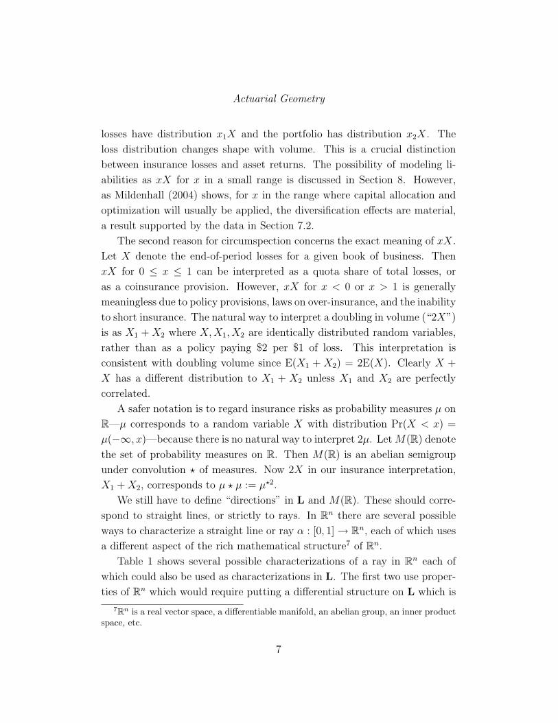
Table 1 shows several possible characterizations of a ray in Rn each of
which could also be used as characterizations in L. The first two use proper-
ties of Rn which would require putting a differential structure on L which is
7Rn is a real vector space, a differentiable manifold, an abelian group, an inner productspace, etc.
7
Actuarial Geometry
Table 1: Possible characterizations of a ray in Rn
Characterization of ray Required structure on Rn
α is the shortest distance betweenα(0) and α(1)
Notion of distance in Rn, differen-tiable manifold
α′′(t) = 0, constant velocity, no ac-celeration
Very complicated on a general man-ifold.
α(t) = tx, x ∈ Rn. Vector space structure
α(s + t) = α(s) + α(t) Can add in domain and range, semi-group structure only.
unnecessarily complicated. The third corresponds to the asset volume/return
model and uses the R vector space structure on Rn. This leaves the fourth
approach: a ray is characterized by α(s + t) = α(s) + α(t). This definition
only requires a semigroup structure (ability to add) for the range space. It
is the definition adopted in Stroock (2003). In L, regarded as a convolution
semigroup, the condition becomes α(s + t) = α(s) ? α(t). Thus we define di-
rections in L using families of random variables satisfying Xs+Xt = Xs+t (or,
equivalently, in M(R) using families of measures µs satisfying µs ?µt = µs+t).
This condition implies that X1 (resp. µ1) is infinitely divisible, that is, for all
integers n ≥ 1 there exists X1/n (resp. µ1/n) so that X = X1/n,1+· · ·+X1/n,n,
(resp. µ1 = µ?n1/n). A general result from probability theory then says that
there exists a Levy process Xt extending X1 to t ∈ R, t ≥ 0, and that µt is
the distribution of Xt. A Levy process is an additive process with indepen-
dent and stationary increments. By providing a basis of directions in L, Levy
processes provide an insurance analog of individual asset return variables.
The insurance analog of an asset portfolio basis becomes a set of Levy
processes representing losses in each line. This definition reflects the fact
that insurance grows account-by-account and that each account adds new
idiosyncratic risk to the total, whereas growing an asset position magnifies
risk which is perfectly correlated with the existing position. Growing in
8
Actuarial Geometry
insurance is equivalent to adding a new asset to a mutual fund, not increasing
an existing stock holding.
This leads us to explore how the total insured loss random variable evolves
volumetrically and temporally. Let the random variable A(x, t) denote aggre-
gate losses from a line with expected annual loss x insured for a time period
t years. Thus A(x, 1) is the annual loss. The central question of this paper
is to describe appropriate models for A(x, t). A Levy process X(t) provides
a good basis for modeling A(x, t). We consider four alternative insurance
models.
IM1. A(x, t) = X(xt). This model assumes there is no difference between
insuring a given insured for a longer period of time and insuring more
insureds for a shorter period.
IM2. A(x, t) = X(xZ(t)), for a subordinator Z(t) with E(Z(t)) = t. Z is
an increasing Levy process which measures random operational time,
rather than calendar time. It allows for systematic time-varying conta-
gion effects, such as weather patterns, inflation and level of economic
activity, affecting all insureds.
IM3. A(x, t) = X(xCt), where C is a mean 1 random variable capturing
heterogeneity and non-diversifiable parameter risk across an insured
population of size x. C could reflect different underwriting positions
by firm, which drive systematic and permanent differences in results.
The variable C is sometimes called a mixing variable.
IM4. A(x, t) = X(xCZ(t)).
All models assume severity has been normalized so that E(A(x, t)) = xt.
Two other models suggested by symmetry, A(x, t) = X(Z(xt)) and A(x, t) =
X(Z(xCt)), are already included in this list because X(Z(t)) is also a Levy
process.
An important statistic describing the behavior of A(x, t) is the coefficient
of variation
υ(x, t) :=
√Var(A(x, t))
xt. (2)
9

Actuarial Geometry
Since insurance is based on the notion of diversification, the behavior of
υ(x, t) as x →∞ and as t →∞ are both of interest. The variance of a Levy
process either grows with t or is infinite for all t. If X(·) has a variance, then
for IM1, υ(x, t) ∝ (xt)−1/2 → 0 as t or x →∞. When υ(x, t) → 0 as t →∞(resp. x → ∞) we will call A(x, t) temporally (resp. volumetrically) diver-
sifying. A process which is both temporally and volumetrically diversifying
will be called diversifying. If X(x) is a standard compound Poisson process
whose severity component has a variance then IM1 is diversifying. Meyers
(2005a) gives evidence that insurance losses are not volumetrically diversify-
ing. In Section 7 we analyze NAIC annual statement data from 1993-2004
and come to the same conclusion. We discuss the behavior of υ across lines of
business as a function of x, and estimate the explicit (and surprising) shape
of the distribution C.
Given a basis of Levy processes we can compute partial derivatives as
∂ρ
∂Xi
= limε→0
ρ(X1(x1) + · · ·+ Xi(xi + ε) + · · ·+ Xn(xn))− ρ(X1(x1) + · · ·+ Xn(xn))
ε(3)
which will generally give different results to the asset model—see Section 4.
Models IM1-4 are all very different to the asset model
AM1. A(x, t) = xX(t)
where X(t) is a return process. X is often modeled using a geometric Brown-
ian motion Hull (1983); Karatzas and Shreve (1988). AM1 is volumetrically
homogeneous, meaning A(kx, t) = kA(x, t). Therefore it has no volumetric
diversification effect whatsoever, since Pr(A(kx, t) < ky) = Pr(A(x, t) < y)
and
υ(x, t) =
√Var(X(t))
t(4)
is independent of x. We discuss some important implications of this in Section
8.
10

Actuarial Geometry
The remainder of the paper is organized as follows. Section 2 shows how
the gradient of a risk measure appears naturally in portfolio optimization
and capital allocation. This highlights the importance of knowing exactly
how partial derivatives with respect to changing volume by line should be
computed. Section 3 discusses Gateaux, or directional, derivatives and dis-
cusses Kalkbrener’s axiomatic allocation. Section 4 shows that the asset view
and actuarial views of portfolio growth give different gradients, using Mey-
ers’ example of “economic” vs. “axiomatic” capital. Section 5 provides an
overview of Levy processes for actuaries. Then Section 6 develops the notion
that Levy processes provide an actuarial straight-line to replace the asset
volume/return model. It describes the set of directions emanating from the
zero variable and computes the directions corresponding to IM1-4 and AM1,
further highlighting the difference between the approaches. Section 7 uses
NAIC annual statement data to provide empirical evidence supporting the
models introduced here. Finally Section 8 revisits the homogeneity assump-
tion of AM1 and Myers and Read (2001) and provides an illustration of how
it is a peculiar special case.
2 THE UBIQUITOUS GRADIENT
Tasche (2000) makes the simple marginal analysis given in the introduction
more rigorous. He shows that the gradient vector of the risk measure ρ is the
only vector suitable for performance measurement, in the sense that it gives
the correct signals to grow or shrink a line of business based on its marginal
profitability and marginal capital consumption8. Tasche’s framework is un-
equivocally financial. As described in the introduction, Tasche considers a
set of basis asset return variables Xi, i = 1, . . . , n and then determines a
portfolio as a vector of asset position sizes x = (x1, . . . , xn) ∈ U ⊂ Rn. The
portfolio value distribution corresponding to x is simply
X = X(x) = X(x1, . . . , xn) =n∑
i=1
xiXi. (5)
8Tasche’s approach is sometimes called a RORAC method, or return on risk-adjustedcapital.
11

Actuarial Geometry
A risk measure on L induces a function ρ : Rn → R. Rather than being
defined on a space of random variables, the induced ρ is defined on (a subset
of) usual Euclidean space using the correspondence between x and a portfolio.
In this context ∂ρ/∂Xi is simply the usual limit
∂ρ
∂xi
= limε→0
ρ(x1, . . . , xi + ε, . . . , xn)− ρ(x1, . . . , xn)
ε. (6)
Eq. 6 is a powerful mathematical notation and it contains two implicit as-
sumptions. First, the fact that we can write xi + ε requires that we can
add in the domain. If ρ were defined on a more general space this may not
possible—or it may involve the convolution of measures rather than addi-
tion of real numbers. Second, and more importantly, adding ε to x in the
ith coordinate unambiguously corresponds to an increase “in the direction”
of the ith asset. This follows directly from the definition in Eq. 5 and is
unquestionably correct in a financial context.
Myers and Read (2001) also assume an asset return/volume model. They
model losses in each line a as La = LaRa where La is the present value of losses
at time 0 and La is the outcome at t = 1 (their notation). This assumption
is essential to their finding that marginal surplus requirements “add-up”.
Irrespective of this assumption, Myers and Read work in the same marginal
return to marginal capital framework as Tasche and as Meyers (2003). They
measure risk and determine capital using a default value, and point out that
marginal default values depend on marginal surplus allocations. Following
Phillips et al. (1998) they argue that, since a firm defaults on all lines if
it defaults on one, marginal surplus requirements should be set so that all
lines’ marginal contributions to default are the same. Again this results in
a surplus requirement proportional to the gradient vector. We re-visit their
result in Section 8
Denault (2001) discusses an axiomatic, game theoretic approach to al-
location. In game theory, the essential property of an allocation is the no-
undercut condition: no collection of lines can be allocated more capital than
it would require on a stand-alone basis. Obviously, if this condition were not
satisfied then the affected lines would want to leave the firm; they are being
12

Actuarial Geometry
“charged” for a supposed diversification benefit. Panjer (2001) also discusses
this approach. Denault assumes the risk measure ρ is coherent, that is, it is
subadditive, positive homogeneous ρ(λx) = λρ(x) for λ ≥ 0, monotonic, and
translation invariant. Combining the homogeneous assumption with Euler’s
theorem he shows that the Aumann-Shapley value is a gradient-based per
unit allocation9.
A theorem of Aubin then shows that if ρ is differentiable its gradient
is the unique per-unit allocation in the core of the coalitional game. The
core is the set of solutions satisfying the no-undercut condition. Thus, under
these assumptions, the gradient provides the unique fair per-unit allocation.
A coalitional game is one where different units can combine in fractional
parts. For insurance, this would correspond to allowing units to quota share
together in different proportions. Since the weights are all between zero and
one, such fractional coalitions still make sense in our insurance setting.
Delbaen (2000a) considers generalizations where ρ is convex but not dif-
ferentiable. Then, elements of the subgradient of ρ (the set of all hyperplanes
which support the graph of ρ) determine fair allocations. When the subgra-
dient contains a single element, the allocation is also given by a Gateaux
derivative, as described in the next section.
Fischer (2003) also works with a portfolio base and uses it to induce a risk
measure on Rn from a measure on Lp. He shows that risk measures which are
everywhere differentiable degenerate to become linear, but shows that non-
trivial risk measures result if the differentiability requirement is weakened
slightly.
It is worth reiterating that risk can be appropriately measured with a
homogeneous risk measure even though the risk process itself is not homoge-
neous. The risk measure must be homogeneous to allow for innocuous things
like changing currency. The problem arises when “risks” are regarded as an
R vector space, because then positive homogeneity becomes close to a linear
requirement: risk is independent of position size. Insurance risk is absolutely
9The Aumann-Shapley value is the integral of the partial derivative of ρ as volumeincreases. Since ρ is 1-homogeneous, Euler’s theorem shows it is constant. The constantderivative is illustrated in Figure 17.
13

Actuarial Geometry
not independent of position size because of diversification between insureds
as volume increases. The scalar in a homogeneous risk measure has a more
restricted meaning for insurance where there is no R vector space structure.
In this context, Fischer’s results are not so surprising. Recent asset modeling
papers, Follmer and Schied (2002); Cheridito et al. (2003), reconsider the de-
sirability of strictly homogeneous risk measures. They introduce the notion
of convex risk measures which include a penalty function for large positions.
3 GATEAUX DERIVATIVES AND
KALKBRENER’S ALLOCATION
The differential represents the best linear approximation to a function in a
given direction. Thus the differential to a function f , at a point x in its
domain, can be regarded as a linear map Dfx which takes a direction, i.e.
tangent vector, at x to a direction at f(x). Exactly what this means will
be discussed more in Section 6. For now it is enough to know that, under
appropriate assumptions, the differential of f at x in direction v, Dxf(v), is
defined by the property
limv→0
f(x + v)− f(x)−Dxf(v)
‖v‖= 0. (7)
The vector v is allowed to tend to 0 from any direction, and Eq. 7 must
hold for all of them. This is called Frechet differentiability. There are several
weaker forms of differentiability defined by restricting the convergence of v
to 0. These include the Gateaux differential, where v = tw with t ∈ R,
t → 0, the directional differential, where v = tw with t ∈ R, t ↓ 0, and the
Dini differential, where v = tw′ for t ∈ R, t ↓ 0, and w′ → w. The function
f(x, y) = 2x2y/(x4 + y4) if (x, y) 6= (0, 0) and f(0, 0) = 0 is not differentiable
at (0, 0), in fact it is not even continuous, but all directional derivatives exist
at (0, 0), and f is Gateaux differentiable.
Kalkbrener (2005) applied Gateaux differentiability to capital allocation.
The Gateaux derivative can be computed without choosing a set of basis
14

Actuarial Geometry
return variables, that is, without setting up a map from Rn → L, provided
it is possible to add in the domain. This is the case for L. The Gateaux
derivative of ρ at Y ∈ L in the direction X ∈ L is defined as
∂ρ
∂X= DρY (X) = lim
ε→0
ρ(Y + εX)− ρ(Y )
ε. (8)
Kalkbrener (2005) shows that if the risk measure ρ satisfies certain ax-
ioms then it can be associated with a unique reasonable capital allocation.
He shows that the allocation is covariance-based if risk is measured using
standard deviation and a co-measure approach when risk is measured by
expected shortfall—so his method is very natural.
Kalkbrener requires an allocation satisfy linear aggregation, diversifica-
tion and continuity axioms, which we describe next. Given a risk measure
ρ, he defines a capital allocation with respect to ρ to be a function Λ of two
variables satisfying Λ(X, X) = ρ(X). Λ(Xi, X) is the capital allocated to Xi
as a sub-portfolio of X. An allocation Λ is linear if it is linear in its first
variable: Λ(aX +bY, Z) = aΛ(X, Z)+bΛ(Y, Z). An allocation is diversifying
if Λ(X, Y ) ≤ Λ(X, X) for all X, so including X in any portfolio does not
increase its risk over a stand-alone portfolio. Finally, Λ is continuous at Y if
limε→0
Λ(X, Y + εX) = Λ(X,Y ) (9)
for all X. Kalkbrener proves that if Λ is a linear, diversifying capital alloca-
tion with respect to ρ and if Λ is continuous at Y then
Λ(X, Y ) = limε→0
ρ(Y + εX)− ρ(Y )
ε(10)
is the Gateaux derivative of ρ at Y in the direction X. Next he uses the Hahn-
Banach theorem to prove that any positively homogeneous, sub-additive risk
measure ρ can be represented as
ρ(X) = maxh(X) | h ∈ Hρ (11)
where Hρ is the set of linear functionals on the space of risks which are dom-
inated by ρ, Hρ = h | h(X) ≤ ρ(X) for all X. The surprising part of this
15

Actuarial Geometry
result is that the max suffices; the supremum is not needed. Using this result,
Kalkbrener defines an allocation associated with a positively homogeneous,
sub-additive risk measure ρ as
Λρ(X, Y ) := hY (X)
where hY ∈ Hρ satisfies hY (Y ) = ρ(Y ). He shows Λρ is linear and diversi-
fying. Finally he shows that for a positively homogeneous, sub-additive risk
measure ρ and risk Y the following are equivalent: (1) that Λρ is continuous
at Y , (2) that the directional derivative
limε→0
ρ(Y + εX)− ρ(Y )
ε(12)
exists for all X, and (3) that there exists a unique h ∈ Hρ with h(Y ) = ρ(Y ).
When these three conditions hold,
Λρ(X, Y ) = limε→0
ρ(Y + εX)− ρ(Y )
ε(13)
for all X. Applying this theory Kalkbrener shows that the unique alloca-
tion for a standard deviation risk measure produces a CAPM-like covariance
allocation, and that an expected shortfall risk measure produces a Phillips-
Sherris like allocation, Phillips et al. (1998); Sherris (2006). Eq. 13 combines
Theorem 18 and Proposition 5 from Delbaen (2000a).
This and the previous section have shown that notions of differentiability
are central to capital allocation. The next section will show that not all the
different notions agree, setting up the need for a better understanding of
“direction” for actuarial random variables that Levy processes will provide.
4 ECONOMIC AND AXIOMATIC CAPITAL
Meyers (2005b) gives an example where Kalkbrener’s “axiomatic” allocation
produces a different result than a marginal business written approach that
is based on a more actuarial set of assumptions. Meyers calls his approach
16

Actuarial Geometry
“economic” since it is motivated by the marginal business added philosophy
discussed in the introduction and Section 2.
The example works with n = 2 independent lines of business and allocates
capital to line 1 in order to keep the notation as simple as possible. Losses
from both lines follow model IM3 with t = 1. The risk measure is standard
deviation ρ(X) = SD(X) for X ∈ L. Xi(xi) is a mixed compound Poisson
variable
Xi(xi) = Si,1 + · · ·+ Si,Ni(xi) (14)
where Ni = Ni(xi) is a Ci-mixed Poisson, so the conditional distribution
N | Ci is Poisson with mean xiCi and the mixing distribution Ci has mean 1
and variance ci. Meyers calls ci the contagion. The mixing distributions are
often taken to be gamma variables, in which case each Ni has a negative bino-
mial distribution. The Si,j, i = 1, 2 are independent, identically distributed
severity random variables. For simplicity, assume that E(Si) = 1, so that
E(Xi(xi)) = E(Ni(xi))E(Si) = xi. Since t = 1 the model only considers
volumetric diversification and not temporal diversification.
We can compute ρ(Xi(xi)) as follows:
ρ(Xi(xi))2 = Var(Xi(xi))
= Var(Ni)E(Si)2 + E(Ni)Var(Si)
= xi(1 + cixi)E(Si)2 + xi(E(S2
i )− E(Si)2)
= cix2i E(Si)
2 + xiE(S2i )
= cix2i + gixi
where gi = E(S2i ). Note that ρ(kX) = kρ(X) for any constant k.
Kalkbrener’s axiomatic capital is computed using the Gateaux directional
derivative, Eq. 13. Let ρi(xi) = ρ(Xi(xi)) and note that ρ((1 + ε)Xi(xi)) =
(1 + ε)ρi(xi). Then, by definition and the independence of X1 and X2, the
17

Actuarial Geometry
Gateaux derivative of ρ at X1(x1) + X2(x2) in the direction X1(x1) is
∂ρ
∂X1
= Λρ(X1(x1), X1(x1) + X2(x2))
= limε→0
ρ(X1(x1) + X2(x2) + εX1(x1))− ρ(X1(x1) + X2(x2))
ε
= limε→0
√(1 + ε)2ρ1(x1)2 + ρ2(x2)2 −
√ρ1(x1)2 + ρ2(x2)2
ε
= limε→0
√ρ1(x1)2 + ρ2(x2)2 + 2ερ1(x1)2 −
√ρ1(x1)2 + ρ2(x2)2
ε
= limε→0
√ρ1(x1)2 + ρ2(x2)2 + 2ερ1(x1)2 −
√ρ1(x1)2 + ρ2(x2)2
2ερ1(x1)2
× limε→0
2ερ1(x1)2
ε
=ρ1(x1)
2
ρ(X1(x1) + X2(x2))
=c1x
21 + g1x1
ρ(X1(x1) + X2(x2)). (15)
This whole calculation has been performed without picking an asset re-
turn basis, but it can be replicated if we do. Specifically, use the Xi(xi)
as a basis and define a linear map of R-vector spaces k : Rn → L, by
(y1, . . . , yn) 7→∑
i yiXi(xi). Let ρk be the composition of k and ρ,
ρk(y1, . . . , yn) = ρ(k(y1, . . . , yn)) = ρ
( ∑i
yiXi(xi)
)=
√∑i
y2i (cix2
i + gixi).
Then∂ρk
∂y1
∣∣∣∣(1,1)
=c1x
21 + g1x1
ρ(X1(x1) + X2(x2))(16)
agreeing with Eq. 15. It is important to remember that yXi(xi) 6= Xi(yxi)
for y 6= 1.
18

Actuarial Geometry
Given the definition of Xi(xi), we can also define an embedding m : Rn →L, by (x1, . . . , xn) 7→
∑i Xi(xi). The map m is a homomorphism of abelian
semigroups but it is not a linear map of real vector spaces because m(kx) 6=km(x). In fact, the image of m will generally be an infinite dimensional real
vector subspace of L. The lack of homogeneity is precisely what produces
a diversification effect. As explained in the introduction and Section 2, an
economic view of capital requires an allocation proportional to the gradient
vector at the margin. Thus capital is proportional to xi∂ρm/∂xi where ρm :
Rn → R is the composition of m and ρ,
ρm(x1, x2) = ρ(m(x1, x2)) =
√∑i
cix2i + gixi. (17)
Since ρm is a function on the reals, we can compute its partial derivative
using standard calculus:
∂ρ
∂x1
=2c1x1 + g1
2ρ(X1(x1) + X2(x2)). (18)
There are two important conclusion: (1) the partial derivatives of ρm and
ρk (which is also the Gateaux derivative of ρ) give very different answers,
Equations 15 and 18, and (2) the implied allocations
c1x21 + g1x1
ρ(X1(x1) + X2(x2))and
2c1x21 + g1x1
2ρ(X1(x1) + X2(x2))(19)
are also different. This is Meyers’ example.
We now think about derivatives in a more abstract way. Working with
functions on Rn obscures some of the complication involved in working on
more general spaces (like L) because the set of directions at any point in
Rn can naturally be identified with Rn. In general this is not the case; the
directions live in a different space. A familiar non-trivial example of this is
the sphere in R3. At each point on the sphere the set of directions, or tangent
vectors, is given by a plane. The collection of different planes, together with
the original sphere, can be combined to give a new object, called the tangent
19

Actuarial Geometry
bundle over the sphere. A point in the tangent bundle consists of a point on
the sphere and a direction, or tangent vector, at that point.
There are several different ways to define the tangent bundle. For the
sphere, an easy method is to set up a local chart, which is a differentiable
bijection from a subset of R2 to a neighborhood of the point. This moves
questions of tangency and direction back into R2 where they are well under-
stood. Charts must be defined at each point on the sphere in such a way that
they overlap consistently, producing an atlas, or differentiable structure, on
the sphere. This is called the coordinate approach.
Another way of defining the tangent bundle is to use curves to define
tangent vectors: a direction becomes the derivative, or velocity vector, of
a curve. The tangent space can be defined as the set of curves through a
point, with two curves identified if they are tangent (agree to degree 1). In
Section 6 we will apply this approach to L. A good general reference on the
construction of the tangent bundle is Abraham et al. (1988).
In this context we see that Kalkbrener and Meyers are computing deriva-
tives with respect to different directions. Kalkbrener is using a direction
defined by the velocity vector of the curve
x 7→ xX (20)
whereas Meyers is using
x 7→ X(x) (21)
for some process X. Note also that the former is a linear map of real vector
spaces whereas the latter is simply a homomorphism of abelian semigroups.
The extra vector space structure makes sense for assets, where it is possible
to change position size and short assets, but not for insurance liabilities. The
appropriate mathematical structure must be driven by the financial realities
of each situation.
20

Actuarial Geometry
5 LEVY PROCESSES FOR ACTUARIES
Levy processes correspond naturally to the set of direction from 0 in L,
as we explained in the introduction. We will now define Levy processes
and then discuss some of their important properties. The next section will
explain the correspondence with directions in more detail. Levy processes
are fundamental to actuarial science, but they are rarely discussed explicitly
in text books. For example, there is no explicit mention of Levy processes in
Beard et al. (1969), Bowers et al. (1986), Daykin et al. (1994), Klugman et al.
(1998), or Panjer and Willmot (1992). However, the fundamental building
block of all Levy processes, the compound Poisson process, is well known
to actuaries. It is instructive to learn about Levy processes in an abstract
manner as they provide a very rich source of examples for modeling actuarial
processes. There are many good textbooks covering the topics described here,
including Feller (1971) volume 2, Breiman (1992), Stroock (1993), Bertoin
(1996), Sato (1999), Barndorff-Nielsen et al. (2001), and Applebaum (2004).
Definition 1 A Levy process is a stochastic process X(t) defined on a prob-
ability space (Ω,F , P) satisfying
LP1. X(0) = 0 almost surely;
LP2. X has independent increments, so for 0 ≤ t1 ≤ · · · ≤ tn+1 the variables
X(tj+1)−X(tj) are independent;
LP3. X has stationary increments, so X(tj+1)−X(tj) has the same distri-
bution as X(tj+1 − tj); and
LP4. X is stochastically continuous, so for all a > 0 and s ≥ 0
limt→s
Pr(|X(t)−X(s)| > a) = 0. (22)
21

Actuarial Geometry
Levy processes are in one-to-one correspondence with the set of infinitely
divisible distributions. Recall that X is infinitely divisible if, for all integers
n ≥ 1, there exist independent, identically distributed random variables Yi
so that X has the same distribution as Y1+ · · ·+Yn. If X(t) is a Levy process
then X(1) is infinitely divisible since X(1) = X(1/n)+(X(2/n)−X(1/n))+
· · ·+(X(1)−X(n−1/n)), and conversely if X is infinitely divisible there is a
Levy process with X(1) = X. In an idealized world, losses should follow an
infinitely divisible distribution because annual losses are the sum of monthly,
weekly, daily, hourly losses10 etc. The Poisson, normal, lognormal, gamma,
Pareto, and Student t distributions are infinitely divisible. The uniform is
not infinitely divisible, nor is any distribution with finite support, nor any
whose moment generating function takes the value zero.
Examples
1. X(t) = kt for a constant k is a trivial Levy process.
2. The Poisson process N(t) with intensity λ has
Pr(N(t) = n) =(λt)n
n!e−λt (23)
for n = 0, 1, . . . .
3. The compound Poisson process X(t) with severity component Z is defined
as
X(t) = Z1 + · · ·+ ZN(t) (24)
where N(t) is a Poisson process.
4. Brownian motion.
5. Let B(t) be a Brownian motion. Then T (t) = infs > 0 | B(s) = t/√
(2)defines a Levy process called the Levy subordinator, which only has positive
jumps. This process is not a compound Poisson process because it has an
infinite number of jumps in any finite period of time. In general, an increasing
process (hence supported on [0,∞)) is called a subordinator.
6. The sum of two Levy processes is a Levy process.
10Predictable fluctuations in frequency from seasonal or daily patterns can be accom-modated using operational time—see Example 7.
22

Actuarial Geometry
7. Lundberg introduced the notion of operational time transforms in order
to maintain stationary increments for compound Poisson distributions. Op-
erational time is a risk-clock which runs faster or slower in order to keep fre-
quency constant. It allows seasonal and daily effects (rush hours, night-time
lulls, etc.) without losing stationary increments. Symbolically, operational
time is an increasing function k : [0,∞) → [0,∞) chosen so that X(k(t))
becomes a Levy process. Any operational time adjustments needed below
are implicit.
8. Let X(t) be a Levy process and let Z(t) be a subordinator, that is, a Levy
process with non-decreasing paths. Then Y (t) = X(Z(t)) is also a Levy
process. This process is called subordination and Y is subordinate to X. Z
is called the directing process. Z is a random operational time.
9. Brownian motion with a drift is an example of a Levy process that is not
a martingale. The process Xt = maxs≤t Bs where Bt is not a Levy process.
It has an infinite number of jumps in some time intervals and none in others.
The characteristic function of a random variable X with distribution µ
is defined as φ(z) = E(eizX) =∫
eizxµ(dx) for z ∈ R. The characteristic
function of a Poisson variable with mean λ is φ(z) = exp(λ(eiz − 1)). The
characteristic function of a compound Poisson process is
φ(z) = E(eizX(t)) = E(E(eizX(t) | N(t))) (25)
= E exp
(N(t) log
∫eizwdν(dw)
)(26)
= exp
(λt
∫(eizw − 1)dν(dw)
)(27)
where ν is the distribution of severity Z. The characteristic equation of a
normal random variable is φ(z) = exp(iµz − σ2z2/2).
We now quote three of the many important results in the theory of Levy
processes. For simplicity we state these in one dimension. See Sato (1999) for
proofs, and for precise statements in higher dimensions. The first theorem,
the famous Levy-Khintchine formula, describes the characteristic function of
an infinitely divisible distribution function µ. The characteristic function of
a general Levy process follows from this.
23

Actuarial Geometry
Theorem 1 (Levy-Khintchine) If the probability distribution µ is infinitely
divisible then its characteristic function has the form
exp
(−σ2z2 +
∫R(eizw − 1− izw1|w|≤1(w))ν(dw) + iγz
)(28)
where ν is a measure on R satisfying ν(0) = 0 and∫
R min(|w|2, 1)ν(dw) < ∞,
and γ ∈ R. The representation by (σ, ν, γ) is unique. Conversely given any
such triple (σ, ν, γ) there exists a corresponding infinitely divisible distribu-
tion.
In Eq. 28, σ is the standard deviation of a Brownian motion component, and
ν is called the Levy measure. The indicator function 1|w|≤1 is present for
technical convergence reasons and is only needed when there are a very large
number of very small jumps. If∫
R min(|w|, 1)ν(dw) < ∞ this term can be
omitted. The resulting γ can then be interpreted as a drift. In the general
case γ does not have a clear meaning as it is impossible to separate drift from
small jumps. The indicator can therefore also be omitted if ν(R) < ∞, and
in that case the inner integral can be written as
ν(R)
∫R(eizw − 1)ν(dw) (29)
where ν = ν/ν(R) is a distribution. Comparing with Eq. 27 shows this term
corresponds to a compound Poisson process.
The triples (σ, ν, γ) in the Levy-Khintchine formula are called Levy triples.
The Levy process X(t) corresponding to the Levy triple (σ, ν, γ) has triple
(tσ, tν, tγ). Define Ψ(z) to be the term in the exponential in Eq. 28. The
characteristic function of X(t) is then exp(tΨ(z)).
The Levy-Khintchine formula helps characterize all subordinators. A
subordinator must have a Levy triple (0, ν, γ) with no diffusion component
and the Levy measure ν must satisfy ν((−∞, 0)) = 0 (no negative jumps) and∫∞0
min(x, 1)ν(dx) < ∞. In particular, this shows there are no non-trivial
continuous increasing Levy processes.
The next theorem describes a decomposition of the sample paths of a
Levy process.
24

Actuarial Geometry
Theorem 2 (Levy-Ito) Let X(t) be a Levy process generated by the Levy
triple (σ, ν, γ). For any measurable G ⊂ (0,∞) × R let J(G) = J(G, ω) be
the number of jumps at time s with height X(s)(ω) − X(s−)(ω) such that
(s, X(s)(ω) − X(s−)(ω)) ∈ G. Then J(G) has Poisson distribution with
mean ν(G) where ν is the measure induced by ν((0, t) × B) = tν(B). If
G1, . . . , Gn are disjoint then J(G1), . . . , J(Gn) are independent. Define
X1(t)(ω) = limε↓0
∫(0,t]×ε<|x|≤1
xJ(d(s, x), ω)− xν(d(s, x))
+
∫(0,t]×|x|>1
xJ(d(s, x), ω). (30)
The process X1 is a Levy process with Levy triple (0, ν, 0). Let
X2(t) = X(t)−X1(t). (31)
Then X2 is a Levy process with Levy triple (σ, 0, γ). The two processes X1, X2
are independent. If∫
R min(|w|, 1)ν(dw) < ∞ then we can define
X3(t)(ω) =
∫(0,t]×R
xJ(d(s, x), ω) (32)
and
X4(t) = X(t)−X3(t). (33)
X3 and X4 are independent Levy processes, with Levy triples (0, ν, 0) and
(σ, 0, γ), and γ is a deterministic drift. X3 is the jump part and X4 is the
continuous part of X.
In Eq. 30 the first term is the compensated sum of small jumps and the
second term is the sum of large jumps. Obviously the cut-off at 1 is arbitrary.
The final theorem we quote shows that compound Poisson processes are the
fundamental building block of Levy processes.
Theorem 3 The class of infinitely divisible distributions coincides with the
class of limit distributions of compound Poisson distributions.
25

Actuarial Geometry
Many properties of a Levy process are time independent, in the sense that
if they are true for one t they are true for all t. For example, the existence
of a moment of order n, being continuous, symmetric, or positive are time
independent. In particular if X(1) has a variance then X(t) has a variance for
all t, and by independent, time homogeneous increments, the variance must
grow with t. This is well-known for Brownian motion, where Var(B(t)) = t,
and a compound Poisson process, where Var(X(t)) = λtE(Z2) and Z is the
severity component.
Next we consider some properties of the models IM1-4. Given a Levy pro-
cess X(t) we defined four models for aggregate losses A(x, t) from a volume
x of insurance, insured for t years:
IM1. A(x, t) = X(xt);
IM2. A(x, t) = X(xZ(t)), for a subordinator Z(t) with E(Z(t)) = t;
IM3. A(x, t) = X(xCt) for a random variables C with E(C) = 1 and
Var(C) = c; and
IM4. A(x, t) = X(xCZ(t)), C and Z(t) independent.
We also defined the asset return/volume model A(x, t) = xX(t). In all cases
severity is normalized so that E(A(x, t)) = xt. Define σ and τ so that
Var(X(t)) = σ2t and Var(Z(t)) = τ 2t. Underwriters tend to avoid risks with
undefined variance, so the assumption of a variance is not onerous!
Models IM3 and IM4 no longer define Levy processes because of the
common C term. Each process has conditionally independent increments,
given C. Thus, these two models no longer assume that each new insured
has losses independent of the existing cohort. We will discuss the impact C
has on the “direction” defined by A in the next section. Example 8 shows
that IM2 is a Levy process.
Table 5 lays out the variance and coefficient of variation υ of these five
models. It also shows whether each model is volumetrically (resp. tempo-
rally) diversifying, that is whether υ(x, t) → 0 as x → ∞ (resp. t → ∞).
26

Actuarial Geometry
Table 2: Variance of IM1-4 and AM
DiversifyingModel Variance υ(x, t) x →∞ t →∞
X(xt) σ2xt σ√xt
Yes Yes
X(xZ(t)) xt(σ2 + xτ 2)
√σ2
xt + τ 2
t No Yes
X(xCt) xt(σ2 + cxt)
√σ2
xt + c No No
X(xCZ(t))x2t2
((c + 1)τ 2
t+ c
)+ σ2xt
√σ2
xt + τ ′2t + c No No
xX(t) x2σ2t σ/√
t Const. Yesτ ′ = (1 + c)τ
The calculations follow easily by conditioning. For example
Var(X(xZ(t))) = EZ(t)(Var(X(xZ(t)))) + VarZ(t)(E(X(xZ(t))))
= E(σ2xZ(t)) + Var(xZ(t))
= σ2xt + x2τ 2t = xt(σ2 + xτ 2).
The characteristics of each model will be tested against NAIC annual state-
ment data in Section 7. We will show that IM1 and AM are not consistent
with the data. With one year of data it is impossible to distinguish between
models IM2-4; for fixed t they all have the same form. Using twelve years
of NAIC data suggests that IM2 and IM4 are not consistent with the data,
leaving model IM3.
The models presented here are one-dimensional. A multi-dimensional
version would use multi-dimensional Levy processes. This allows for the
possibility of correlation between lines. In addition, correlation between lines
can be induced by using correlated mixing variables C. This is the common-
shock model, described in Meyers (2005a).
27

Actuarial Geometry
5.1 LEVY PROCESSES AND CATASTROPHEMODEL PMLs
Since Hurricane Andrew in 1992 computer simulation models of hurricane
and earthquake insured losses have developed into an essential tool for in-
dustry risk assessment and management. The output from these models
specifies a compound Poisson Levy process. Given the interest surrounding
the use of these models, this section will translate some common industry
terms, such as return period and probable maximum loss (PML), into precise
formulae.
PML and maximum foreseeable loss (MFL) are terms from individual
risk property underwriting which far pre-date modern computer simulation
models. The PML is an estimate of the largest loss that a building or a
business in the building is likely to suffer, considering the existing mitigation
features, because of a single fire. The PML assumes that critical protection
systems are functioning as expected. The MFL is an estimate of the largest
fire loss likely to occur if loss-suppression systems fail. For a large office
building the PML is sometimes estimated as a total loss of 4 to 6 floors,
assuming the fire itself would be contained to one or two floors. The MFL
can be estimated as a total loss “within four walls”, so a single structure burns
down. These terms are now over-loaded with different meanings related to
catastrophe modeling. McGuinness (1969) discusses meanings of the term
PML.
Simulation models produce a sample of n loss events, each with an associ-
ated annual frequency λi and expected event loss li, i = 1, . . . , n. Each event
is assumed to have a Poisson occurrence frequency distribution. The associ-
ated Levy measure ν is concentrated on the set l1, . . . , ln with ν(li) = λi.
Since the models only simulate a finite number of events, ν(R) =∑
i λi < ∞.
Let λ = ν(R) be the total modeled event frequency. We can normalize to get
an event severity distribution ν = ν/λ because λ < ∞. Let Xt be the Levy
process associated with the Levy triple (0, ν, 0).
Catastrophe risk is usually managed using reinsurance purchased on an
occurrence basis; it covers all losses from a single event. Therefore companies
28

Actuarial Geometry
are interested in the annual frequency of events above a threshold. Using the
Levy measure ν, the annual frequency of losses greater than or equal to x is
simply λ(x) := ν([x,∞)), which, by definition, is
λ(x) = ν([x,∞)) =∑li≥x
λi. (34)
Since λ(x) is the annual frequency for a loss of size ≥ x, and each event
frequency has a Poisson distribution, the (exponentially distributed) waiting
time for such a loss has mean 1/m(x). Surprisingly, this is not what is usually
referred to as the “return period”.
Using the Poisson count distribution, the annual probability of one or
more single events in a year causing loss ≥ x is the probability that a Poisson
variable N with mean λ(x) has value 1 or more, that is
Pr(N ≥ 1) = 1− Pr(N = 0) = 1− exp(−λ(x)). (35)
Therefore the probability of one or more occurrences causing ≥ x loss is
1 − exp(−λ(x)). The return period of this loss is then generally quoted
as 1/(1 − exp(−λ(x))). For large enough x, λ(x) is very small and 1/(1 −exp(−λ(x))) is approximately 1/λ(x).
Insurance companies are also interested in percentiles of X1—especially
after the hurricane seasons of 2004 and 2005! These percentiles are called
“aggregate PML” points. In this context, the return period is again the re-
ciprocal of the percentile point. Aggregate PMLs have two disadvantages:
they are hard to compute and they do not correspond to how insurers usu-
ally manage risk. They are, however, clearly important for Enterprise Risk
Management.
It should now be clear that a statement such as “the 100 year PML loss
is $200M” is inherently ambiguous. Insurance companies have used this to
their benefit. For example, one company announced
Hurricane Katrina is the costliest catastrophe in the United States
history. The single event probability of the industry experienc-
ing losses at or above the Katrina level as a result of a hurricane
hitting in the specific area where Katrina made landfall was 0.2%
based on the AIR Worldwide Corporations catastrophe model,
which is equivalent to a one in 500 year event. [Emphasis added]
29
Actuarial Geometry
This is a true statement—regarding a subset of the total simulated events.
Perhaps losses x1, . . . , xm of the n simulated hit the “specific area where
Katrina made landfall”, for some m n. The quoted PML statement
refers to using a Levy measure ν ′ supported just on these events. Other
press releases spoke of Katrina being a 250 year event, or higher, for the
industry. Again, these statements could be true if the sample space of events
is suitably constrained, but they are manifestly not true of Katrina as an
industry hurricane event. On an industry basis Katrina is around a 25-
50 year event—one can count Andrew, the Long Island storm of 1938, and
Katrina as broadly comparable events in the last 100 years alone.
6 “DIRECTIONS” IN THE SPACE OF
ACTUARIAL RANDOM VARIABLES
This section combines three threads we have already discussed to produce a
description of “directions” in the space L. The first is the notion that direc-
tions, or tangent vectors, live in a separate space called the tangent bundle.
The tangent bundle can be identified with the original space in the case
of Rn—a simplification which confuses intuition in more involved examples.
The second thread comes from regarding tangent vectors as velocity vectors of
curves. The third uses the idea presented in the introduction that Levy pro-
cesses, characterized by the additive relation X(s+t) = X(s)+X(t), provide
the appropriate analog of straight lines or rays. The program is, therefore,
to compute the derivative of the curve t 7→ X(t) at t = 0. The ideas pre-
sented here are part of an elegant general theory of Markov processes. The
presentation follows the beautiful book by Stroock (2003). Before getting
into the details we review a schematic of the difference between the Meyers
and Kalkbrener maps ρm and ρk, and then describe a finite sample space
version of L which illustrates the difficulties involved in regarding it as a dif-
ferentiable manifold. Throughout the section it is more convenient to work
with distribution functions µt than random variables X(t); the connection
between the two is µt(B) = Pr(X(t) ∈ B) for a measurable set B.
30

Actuarial Geometry
0
1
X=m(1)
k'(1)
m'(1)
k and m
x m(x)
R+Space of risks
m(0)=0
k(x)=xX
Figure 1: Levy process and homogeneous embeddings of R+ into L. TheLevy process embedding corresponds to the straight line.
The difference between the maps m(x) = X(x) and k(x) = xX lies in the
meaning of “in the direction X”. Kalkbrener takes it to mean adding a small
extra amount εXi, perfectly correlated to the existing Xi, to the portfolio.
This makes sense for an asset portfolio but not for an portfolio of insurance
risks. Each insured risk is unique; laws and contractual provisions forbid
insuring the exact same risk twice—or even (1 + ε) times. Meyers’ model
and IM1-4 recognize that insurance volume increases either by insuring more
individuals (increase x), or insuring the same individuals for a longer period
of time (increasing t). Eq. 14 recognizes the increase by increasing the claim
count.
Figure 1 is a schematic of the difference between m and k. It shows
the map m from R+ → L, the space of risks; the image of m is shown
as a straight line. X := m(1) is the image of 1. The tangent vector,
m′(1), to the embedding m is shown extending along the direction of the
line; this is the natural direction to interpret as “growth in the direction
X”. In the schematic, the embedding k is shown as the curved line. The
31

Actuarial Geometry
tangent vector k′(1) is not pointing in the same direction as m′(1). For
a risk measure ρ, ∂ρ/∂X is the evaluation of the linear differential map
Dρ on a tangent vector in the direction X. Meyer’s embedding m corre-
sponds to ∂(ρ m)/∂t|t=1 = DρX(m′(1)) whereas Kalkbrener’s corresponds
to ∂(ρ k)/∂t|t=1 = DρX(k′(1)). As demonstrated in Section 4 these are not
the same—just as the schematic leads us to expect. The difference between
k′(1) and m′(1) is a measure of the diversification benefit given by m com-
pared to k. k maps x 7→ xX and so offers no diversification to an insurer.
Again, this is correct for an asset portfolio (you don’t diversify a portfolio by
buying more of the same stock) but it is not true for an insurance portfolio.
In order to see that the construction of tangent directions in L may not
be trivial, consider the space M of probability measures on Z/n, the integers
0, 1, . . . , n− 1 with + given by addition modulo n. An element µ ∈ M can
be identified with an n-tuple of non-negative real numbers p0, . . . , pn−1 satis-
fying∑
i pi = 1. Thus elements of M are in one to one correspondent with ele-
ments of the n dimensional simplex ∆n = (x0, . . . , xn−1) |∑
i xi = 1 ⊂ Rn.
∆n inherits a differentiable structure from Rn; we already know how to think
about directions and tangent vectors in Euclidean space. However, even
thinking about ∆3 ⊂ R3 shows M is not an easy space to work with. ∆3 is a
plane triangle; it has a boundary of three edges and each edge has a bound-
ary of two vertices. The tangent spaces at each of these boundary points
is different and different again from the tangent space in the interior of ∆3.
As n increases the complexity of the boundary increases and, to compound
the problem, every point in the interior gets closer to the boundary. For
measures on R the boundary is dense.
Now let M be the space of probability measures on R and let δx ∈ M
be the measure giving probability 1 to x ∈ R. We will describe the space
of tangent vectors to M at δ0. By definition, all Levy processes X(t) have
distribution δ0 at t = 0. Measures µt ∈ M are defined by their action on
functions f on R. Let 〈f, µ〉 =∫
R f(x)µ(dx). In view of the fundamental
theorem of calculus, the derivative µt of µt should satisfy
〈f, µt〉 − 〈f, µ0〉 =
∫ t
0
µτfdτ, (36)
32

Actuarial Geometry
indicating µt is a functional acting on f . Converting Eq. 36 to its differential
form suggests that
µtf(0) = limt↓0
〈f, µt〉 − 〈f, µ0〉t
(37)
= limt↓0
E(f(X(t)))− E(f(X(0)))
t(38)
where X(t) has distribution µt.
We now consider how this formula works when X(t) is related to a Brow-
nian motion or a compound Poisson—the two building block Levy processes.
Suppose first that X(t) is a Brownian motion with drift γ and standard de-
viation σ, so X(t) = γt + σB(t) where B(t) is a standard Brownian motion.
Let f be a function with a Taylor’s expansion about 0. We can compute
µ0f(0) = limt↓0
[E(f(0) + X(t)f ′(0) +X(t)2f ′′(0)
2+ O(t2))− f(0)]/t (39)
= limt↓0
[γtf ′(0) +σ2tf ′′(0)
2+ O(t2))]/t (40)
= γf ′(0) +σ2f ′′(0)
2, (41)
because E(X(t)) = E(γt + σB(t)) = γt, E(X(t)2) = γ2t2 + σ2t, E(B(t)) = 0
and E(B(t)2) = t. Thus µ0 acts as a second order differential operator
µ0 = γd
dx+
σ2
2
d2
dx2. (42)
Next suppose that X(t) is a compound Poisson distribution with Levy mea-
sure ν, ν(0) = 0 and λ = ν(R) < ∞. Let J be a variable with distribution
ν/λ, so, in actuarial terms, J is the severity. The number of jumps of X(t)
follows a Poisson distribution with mean λt. If t is very small then the ax-
ioms characterizing the Poisson distribution imply that there is a single jump
with probability λt and no jump with probability 1− λt. Conditioning on a
33

Actuarial Geometry
jump E(f(X(t))) = (1− λt)f(0) + λtE(f(J)) and so
µ0f(0) = limt↓0
E(f(X(t)))− E(f(X(0)))
t(43)
= limt↓0
λt(E(f(J))− f(0))
t(44)
= λ(E(f(J))− f(0)) (45)
=
∫f(y)− f(0)ν(dy) (46)
This analysis side-steps some technicalities by assuming that ν(R) < ∞.
Combining these two results makes the following theorem plausible.
Theorem 4 (Stroock (2003) Thm 2.1.11) There is a one-to-one corre-
spondence between directions, or tangent vectors, in M and Levy processes.
If µt is a Levy process characterized by Levy triple (σ, ν, γ) then µt is the
linear operator acting on f by
µtf(z) = γdf
dx+
1
2σ2d2f
dx2+
∫R
f(y + z)− f(z)− df
dx
y
1 + |y|2ν(dy) (47)
As in the Levy-Khintchine theorem, the extra term in the integral is needed
for technical convergence reasons when there is a large number of very small
jumps.
We can now compute the difference between the directions implied by
each of IM1-4 and AM. This quantifies the difference between m′(1) and
k′(1) in Figure 1. In order to focus on the models that realistically can be
used to model insurance losses we will assume γ = σ = 0 and ν(R) < ∞.
Assume the Levy triple for the subordinator Z is (0, ρ, 0). Also E(C) = 1,
Var(C) = c, and C, X and Z are all independent.
For each model we can consider the time derivative or the volume deriva-
tive. There are obvious symmetries between these two for IM1 and IM3. For
IM2 the temporal derivative is the same as the volumetric derivative of IM3
with C = Z(t).
34

Actuarial Geometry
Theorem 4 gives the direction for IM1 as corresponding to the operator
Eq. 47 multiplied by x or t as appropriate. For example, the time direction
is given by the operator
µ0f(z) = x
∫f(z + y)− f(z)ν(dy). (48)
The temporal derivative of IM2, X(xZ(t)), is more tricky. Let K have
distribution ρ/ρ(R), the severity of Z. For small t, Z(t) = 0 with probability
1− ρ(R)t and Z(t) = K with probability ρ(R)t. Thus
µ0f(z) = ρ(R)E(f(z + X(xK))− f(z)) (49)
=
∫(0,∞)
∫(0,∞)
f(z + xy)− f(z)νxk(dy)ρ(dk) (50)
where νk is the distribution of X(k). This has the same form as IM1, except
the underlying Levy measure ν has been replaced with
ν ′(B) =
∫(0,∞)
νk(B)ρ(dk). (51)
For IM3, X(xCt), the direction is the same as for model IM1. This is
not a surprise because the effect of C is to select, once and for all, a random
speed along the ray; it does not affect its direction. By comparison, in model
IM2 the “speed” is proceeding by jumps, but again, the direction is fixed. If
E(C) 6= 1 then the derivative would be multiplied by E(C).
Finally the volumetric derivative of the asset model is simply
µ′0f(z) = X(t)df
dx. (52)
Thus the derivative is the same as for a deterministic drift Levy process.
This should be expected since once X(t) is known it is fixed regardless of
volume x. Comparing with the derivatives for IM1-4 expresses the different
directions represented schematically in Figure 1 analytically. The result is
also reasonable in light of the different shapes of tZ and√
tZ as t → 0, for
a random variable Z with mean and standard deviation equal to 1. For very
35

Actuarial Geometry
• From C:\SteveBase\papers\CapitalAllocation\TeX\Tables etc..xls
0
0.050
0.100
0.150
0.200
-0.60 -0.40 -0.20 0 0.20 0.40 0.60
0.05
Sqrt(0.05)
0.01
Sqrt(0.01)
Figure 2: Illustration of the difference between tZ and√
tZ for Z a standardnormal as t → 0.
small t, tZ is essentially the same as a deterministic tE(Z), whereas√
tZ has
a standard deviation√
t which is much larger than the mean t. Its coefficient
of variation 1/√
t →∞ as t → 0. The relative uncertainty in√
tZ grows as
t → 0 whereas for tZ it disappears. This is illustrated in Figure 2.
Severity uncertainty is another interesting form of uncertainty. Suppose
that claim frequency is still λ but that severity is given by a family of mea-
sures νV for a random V . Now, in each state, the Levy process proceeds
along a random direction defined by V (ω), so the resulting direction is a
mixture
µ0 =
∫µ0,vdµ(v) (53)
where µ is the distribution of V .
It is interesting to interpret these results from the perspective of credibil-
ity theory. Credibility is usually associated with repeated observations of a
given insured, so t grows but x is fixed. For models IM1-4 severity (direction)
is implicitly known. For IM2-4 credibility determines information about the
36

Actuarial Geometry
fixed (C) or variable (Z(t)) speed of travel in the given direction. If there
is severity uncertainty, V , then repeated observation resolves the direction
of travel, rather than the speed. Obviously both direction and speed are
uncertain in reality.
It may be possible and enlightening for actuaries to model directly with a
Levy measure ν and hence avoid the artificial distinction between frequency
and severity. Catastrophe models already work in this way. Several aspects
of actuarial practice could benefit from avoiding the frequency/severity di-
chotomy. Explicitly considering the count density of losses by size range helps
clarify the effect of loss trend. In particular, it allows different trend rates
by size of loss. Risk adjustments become more transparent. The theory
of risk adjusted probabilities for compound Poisson distributions, Delbaen
and Haezendonck (1989); Meister (1995), is more straightforward if loss rate
densities are adjusted without the constraint of adjusting a severity curve
and frequency separately. This approach can be used to generate state price
densities directly from catastrophe model output. Finally, the Levy mea-
sure is equivalent to the log of the aggregate distribution, so convolution of
aggregates corresponds to a pointwise addition of Levy measures. This sim-
plification is clearer when frequency and severity are not split. It facilitates
combining losses from portfolios with different policy limits.
This section has shown there are important local differences between the
maps k and m. They may agree at a point, but the agreement is not first
order—the two maps define different directions. Since capital allocation relies
on derivatives—the ubiquitous gradient—it is not surprising that different
allocations result. This is shown in practice by Meyer’s example and by the
failure of Myers and Read’s formula to add-up for diversifying Levy processes.
7 EMPIRICAL EVIDENCE: VOLUMETRIC
AND TEMPORAL EVOLUTION OF
PORTFOLIOS
NAIC annual statement accident year schedule P data from 1993 to 2004 by
line of business can be modeled using IM1-4. The model fits can differentiate
37

Actuarial Geometry
company effects from accident year pricing cycle effects, and the parameters
show considerable variation by line of business. Importantly, the fits can
capture information about the mixing distribution C, based on Proposition
1, below.
Three hypotheses will be tested from the previous sections: (1) that the
asymptotic coefficient of variation or volatility11 as volume grows is strictly
positive; (2) that time and volume are symmetric in the sense that υ(x, t) =
CV(A(x, t)) only depends on xt; and (3) that the data is consistent with
model IM3. IM3 implies that diversification over time follows a symmetric
modified square root rule, υ(x, t) =√
(σ2/xt) + c.
7.1 THEORY
Consider an aggregate loss distribution with a C-mixed Poisson frequency
distribution, per Eq. 14. If the expected claim count is large and if the
severity has a variance then particulars of the severity distribution diversify
away in the aggregate. Any severity from a policy with a limit has a vari-
ance; unlimited directors and officers on a large corporation may not have a
variance. Moreover the variability from the Poisson claim count component
also diversifies away and the shape of the normalized aggregate loss distri-
bution, aggregate losses divided by expected aggregate losses, converges in
distribution to the mixing distribution C.
These assertions can be proved using moment generating functions. Let
Xn be a sequence of random variables with distribution functions Fn and let
X another random variable with distribution F . If Fn(x) → F (x) as n →∞for every point of continuity of F then we say Fn converges weakly to F and
that Xn converges in distribution to X.
Convergence in distribution is a relatively weak form of convergence.
A stronger form is convergence in probability, which means for all ε > 0
Pr(|Xn − X| > ε) → 0 as n → ∞. If Xn converges to X in probabil-
ity then Xn also converges to X in distribution. The converse is false.
For example, let Xn = Y and X be binomial 0/1 random variables with
11Volatility of loss ratio is used to mean coefficient of variation of loss ratio.
38

Actuarial Geometry
Pr(Y = 1) = Pr(X = 1) = 1/2. Then Xn converges to X in distribu-
tion. However, since Pr(|X − Y | = 1) = 1/2, Xn does not converge to X in
probability.
Xn converges in distribution to X if the moment generating functions
(MGFs) Mn of Xn converge to the MGF of M of X for all z: Mn(z) → M(z)
as n →∞, see (Feller, 1971, Volume 2, Chapter XV.3 Theorem 2). We can
now prove the following proposition.
Proposition 1 Let N be a C-mixed Poisson distribution with mean n, C
with mean 1 and variance c, and let X be an independent severity with mean
x and variance x(1 + γ2). Let A = X1 + · · · + XN and a = nx. Then the
normalized loss ratio A/a converges in distribution to C, so
Pr(A/a < α) → Pr(C < α) (54)
as n →∞. Hence
σ(A/a) =
√c +
x(1 + γ2)
a→√
c. (55)
Proof: The moment generating function MA(z) of A is
MA(z) = MC(n(MX(z)− 1)) (56)
where MC and MX are the moment generating functions of C and X. Using
Taylor’s expansion we can write
limn→∞
MA/a(z) = limn→∞
MA(z/a)
= limn→∞
MC(n(MX(z/nx)− 1))
= limn→∞
MC(n(M ′X(0)z/nx + R(z/nx)))
= limn→∞
MC(z + nR(z/nx)))
= MC(z)
for some remainder function R(z) = O(z2). The assumptions on the mean
and variance of X guarantee M ′X(0) = x = E(X) and that the remainder
term in Taylor’s expansion is O(z2). The second part is trivial.
39

0 0.2 0.4 0.6 0.8 1 1.2 1.4 1.6 1.8 20
5
10
15
20
25
30
35
0 0.2 0.4 0.6 0.8 1 1.2 1.4 1.6 1.8 20
0.5
1
1.5
2
0 0.2 0.4 0.6 0.8 1 1.2 1.4 1.6 1.8 20
2
4
6
8
10
Figure 3: Theoretical distribution of scaled aggregate losses with no param-eter or structure uncertainty and Poisson frequency.
0 0.2 0.4 0.6 0.8 1 1.2 1.4 1.6 1.8 20
5
10
15
20
25
30
35
0 0.2 0.4 0.6 0.8 1 1.2 1.4 1.6 1.8 20
0.5
1
1.5
2
0 0.2 0.4 0.6 0.8 1 1.2 1.4 1.6 1.8 20
2
4
6
8
10 Figure 4: Theoretical distribution envelope of scaled aggregate losses with agamma mixed Poisson frequency with mixing variance c = 0.0625.

Actuarial Geometry
The proposition implies that if the frequency distribution is actually a
Poisson, so the mixing distribution C is C = 1 with probability 1, then
the loss ratio distribution of a very large book will tend to the distribution
concentrated at the expected. Hence the expression “with no parameter risk
the process risk completely diversifies away.”
Figures 3 and 4 illustrate the proposition, showing how the aggregate
distributions change shape as expected counts increase. In Figure 3, C = 1
and the claim count is Poisson. Here the scaled distributions get more and
more concentrated about the expected value (scaled to 1.0). In Figure 4,
C has a gamma distribution with variance 0.0625 (asymptotic CV of 25%).
Now the scaled aggregate distributions converge to C.
The proposition shows that in many realistic insurance situations severity
is irrelevant to the shape of the distribution of aggregate losses for a large
book of business. This is an irritating but important result. Severity distri-
butions are relatively easy to estimate, particularly when occurrence severity
is limited by policy terms and conditions. Frequency distributions, on the
other hand, are much more difficult to estimate. This proposition shows that
the single most important variable for estimating the shape of A is the mix-
ing distribution C. Problematically, C is never independently observed! The
power of the proposition is to suggest a method for determining C: consider
the loss ratio distribution of large books of business. We now do this using
the NAIC annual statement data.
7.2 EMPIRICAL EVIDENCE—VOLUMETRIC
We use data from property-casualty NAIC annual statements to apply the
above theory and determine an appropriate distribution for C (or Z(1)).
This provides new insight into the exact form of “parameter risk”. In the
absence of empirical information, mathematical convenience usually reigns
and a gamma distribution is used for C; the unconditional claim count is then
a negative binomial. The distribution of C is called the structure function in
credibility theory, Buhlmann (1970).
Schedule P in the property-casualty annual statement includes a ten
accident-year history of gross, ceded and net premiums and ultimate losses
41

Actuarial Geometry
Table 3: Characteristics of Various Lines of Insurance
Line Homogeneity Regulation Limits Cycle CatsPers Auto High High Low Low NoComm Auto Moderate Moderate Moderate High NoWork Comp Moderate High Statutory High PossibleMed Mal Moderate Moderate Moderate High NoComm MP Moderate Moderate Moderate High ModerateOther Liab Occ Low Low High High YesHomeowners Moderate High Low Low HighOther Liab CM Low Low High High Possible
by major line of business. We focus on gross ultimate losses. The ma-
jor lines include private passenger auto liability, homeowners, commercial
multi-peril, commercial auto liability, workers compensation, other liability
occurrence (premises and operations liability), other liability claims made
(including directors and officers and professional liability but excluding med-
ical), and medical malpractice claims made. These lines have many distin-
guishing characteristics that are subjectively summarized in Table 3. In the
table, homogeneity refers to the consistency in terms and conditions within
the line. The two other liability lines are catch-all classifications including a
wide range of insureds and policies. Regulation indicates the extent of rate
regulation by the states’ insurance departments. Limits refers to the typical
policy limit. Personal auto liability limits rarely exceed $300,000 per accident
and are characterized as low. Most commercial lines policies have a primary
limit of $1M, possibly with excess liability policies above that. Workers com-
pensation policies do not have a limit but the benefit levels are statutorily
prescribed by each state. Cycle is an indication of the extent of the pricing
cycle in each line; it is simply split personal (low) and commercial (high).
Finally, cats covers the extent to which the line is subject to multi-claimant,
single occurrence catastrophe losses such as hurricanes, earthquakes, mass
tort, securities laddering, terrorism and so on. The data is interpreted in the
light of these characteristics.
In order to apply Proposition 1 we proxy a “large” book as one with
more than $100M of premium in each accident year. Figure 5 shows how
42

All Lines
0
0.20
0.40
0.60
0.80
1.00
1.20
0 5.0B 10.0B 15.0B 20.0BPremium
CV
Los
s R
atio 0.10
1.00
1M 10M 100M 1,000M 10,000M
100,000M
Commercial Auto
0
0.20
0.40
0.60
0.80
1.00
1.20
0 0.5B 1.0B 1.5B 2.0BPremium
CV
Los
s R
atio
0.10
1.00
1M 10M 100M 1,000M 10,000M
Commercial Multiperil
0
0.20
0.40
0.60
0.80
1.00
1.20
0 0.5B 1.0B 1.5B 2.0B 2.5BPremium
CV
Los
s R
atio
0.10
1.00
1M 10M 100M 1,000M 10,000M
Homeowners
0
0.20
0.40
0.60
0.80
1.00
1.20
0 2.0B 4.0B 6.0B 8.0B 10.0B 12.0BPremium
CV
Los
s R
atio 0.10
1.00
1M 10M 100M 1,000M 10,000M
100,000M
Private Passenger Auto
0
0.20
0.40
0.60
0.80
1.00
1.20
0 5.0B 10.0B 15.0B 20.0BPremium
CV
Los
s R
atio 0.10
1.00
1M 10M 100M 1,000M 10,000M
100,000M
Workers Compensation
0
0.20
0.40
0.60
0.80
1.00
1.20
0 1.0B 2.0B 3.0B 4.0BPremium
CV
Los
s R
atio
0.10
1.00
1M 10M 100M 1,000M 10,000M
Medical Malpractice CM
0
0.20
0.40
0.60
0.80
1.00
1.20
0 0.1B 0.2B 0.3B 0.4B 0.5B 0.6B 0.7BPremium
CV
Los
s R
atio
0.10
1.00
1M 10M 100M 1,000M
Other Liability Occurrence
0
0.20
0.40
0.60
0.80
1.00
1.20
0 0.5B 1.0B 1.5B 2.0B 2.5BPremium
CV
Los
s R
atio
0.10
1.00
1M 10M 100M 1,000M 10,000M
Other Liability CM
0
0.20
0.40
0.60
0.80
1.00
1.20
0 0.5B 1.0B 1.5B 2.0B 2.5BPremium
CV
Los
s R
atio
0.10
1.00
1M 10M 100M 1,000M 10,000M
Figure 5: The relationship between raw loss ratio volatility, measured ascoefficient of variation of loss ratios, and premium volume, using data fromaccident years 1993-2004. Each inset graph plots the same data on a log/logscale, showing that the volatility continues to decrease materially for pre-mium volumes in the $100M’s. The total line is distorted by changing mixof business by volume; the largest companies are dominated by private pas-senger auto liability which is the lowest volatility line.

Actuarial Geometry
the volatility of loss ratio by line varies with premium size. It is computed
by bucketing schedule P loss ratios by premium size band and computing
the volatilities in each bucket. Each inset chart shows the same data on a
log/log scale. The figure shows three things: (1) that the loss processes are
not volumetrically diversifying, that is the volatility does not decrease to
zero with volume; (2) that below a range $100M-1B (varying by line) there
are material changes in volatility with premium size; and (3) that $100M
is a reasonable threshold for large, in the sense that there is less change in
volatility beyond $100M. The second point means that the inhomogeneity in
a loss portfolio is material in the range where most companies would try to
set profit targets by line or business unit. This is consistent with Mildenhall
(2004) and is also discussed in Section 8.
We now determine C by line by applying Proposition 1. The data consists
of observed schedule P gross ultimate loss ratios λc,y by company c and
accident year y = 1993, . . . , 2004. The observation λc,y is included if company
c had gross earned premium ≥ $100M in year y. The data is in the form of
an unbalanced two-way ANOVA table with at most one observation per cell.
Let λ.,. denote the average loss ratio over all companies and accident years,
and λc,. (resp. λ.,y) the average loss ratio for company c over all years (resp.
accident year y over all companies). Each average can be computed as a
straight arithmetic average of loss ratios or as a premium-weighted average.
With this data we will determine four different measures of volatility.
Res1. Raw loss ratio volatility across all twelve years of data for all com-
panies. This volatility includes a pricing cycle effect, captured by
accident year, and a company effect.
Res2. Control for the accident year effect λ.,y. This removes the pricing cycle.
It also removes some of the catastrophic loss effect for a year. In the
sample data this causes problems with the results for homeowners in
2004.
Res3. Control for the company effect λc,.. This removes spurious loss ratio
variation caused by differing expense ratios, distribution costs, profit
targets, classes of business, limits, policy size and so forth.
44

Actuarial Geometry
Res4. Control for both company effect and accident year, i.e. perform an
unbalanced two-way ANOVA with zero or one observation per cell.
This can be done additively, modeling the loss ratio λc,y for company
c in year y as
λc,y = λ.,. + (λc,. − λ.,.) + (λ.,y − λ.,.), (57)
or multiplicatively as
λc,y = λ.,.(λc,./λ.,.)(λ.,y/λ.,.). (58)
The multiplicative approach is generally preferred as it never produces
negative fit loss ratios. The statistical properties of the residual dis-
tributions are similar for both forms.
Using Proposition 1 we obtain four estimates for the distribution of C
from the empirical distributions of λc,y/λ.,., λc,y/λ.,y, λc,y/λc,. and λc,y/λc,y
for suitably large books of business. The additive residuals λc,y − λc,y also
have a similar distribution (not shown).
Figures 6-8 show analyses of variance for the model described by Eq. 57.
Because the data is unbalanced, consisting of at most one observation per
cell, it is necessary to perform a more subtle ANOVA than in the balanced
case. We follow the method described in (Ravishanker and Dey, 2002, Sec-
tion 9.2.2). The idea is to adjust for one variable first and then to remove
the effect of this adjustment before controlling for the other variable. For
example, in the extreme case where there is only one observation for a given
company, that company’s loss ratio is fit exactly with its company effect and
the loss ratio observation should not contribute to the accident year volatil-
ity measure. Both the accident year effect and the company effect are highly
statistically significant in all cases, except the unadjusted company effect for
homeowners and the adjusted company effect for other liability claims made.
The R2 statistics are in the 50-70% range for all lines except homeowners.
As discussed above, the presence of catastrophe losses in 2004 distorts the
homeowners results.
45

Additive ANOVA for Commercial Auto, $100M ThresholdSource of Variation Sum of Squares D of F Mean Squares F Ratio p ValueUnadjusted Accident Year 6.3446 11 0.5768 37.2271 6.70E-55 ***Adjusted Company Effect 4.9147 56 0.0878 5.6645 3.44E-26 ***Residual 5.7658 407 0.0142 Std. Deviation 11.9%
Total (about mean) 17.0251 474 0.0359 Std. Deviation 19.0%R2 0.6613
Adjusted Accident Year 5.0773 11 0.4616 29.7914 8.48E-46 ***Unadjusted Company Effect 6.1819 56 0.1104 7.1250 3.14E-34 ***
Tukey's Test for InteractionsSSA 0.0035 F statistic 0.2443SSB 5.7658 p Value 0.621SSR 5.7624
Additive ANOVA for Commercial Multiperil, $100M ThresholdSource of Variation Sum of Squares D of F Mean Squares F Ratio p ValueUnadjusted Accident Year 7.3649 11 0.6695 21.3469 1.85E-34 ***Adjusted Company Effect 7.9119 67 0.1181 3.7650 5.72E-17 ***Residual 12.0741 420 0.0287 Std. Deviation 17.0%
Total (about mean) 27.3509 498 0.0549 Std. Deviation 23.4%R2 0.5585
Adjusted Accident Year 9.4834 11 0.8621 27.4873 4.09E-43 ***Unadjusted Company Effect 5.7934 67 0.0865 2.7569 3.68E-10 ***
Tukey's Test for InteractionsSSA 0.0277 F statistic 0.9668SSB 12.0741 p Value 0.326SSR 12.0464
Additive ANOVA for Homeowners, $100M ThresholdSource of Variation Sum of Squares D of F Mean Squares F Ratio p ValueUnadjusted Accident Year 3.0722 11 0.2793 3.1671 3.67E-04 ***Adjusted Company Effect 12.9407 78 0.1659 1.8813 3.39E-05 ***Residual 42.7530 488 0.0876 Std. Deviation 29.6%
Total (about mean) 58.7659 577 0.1018 Std. Deviation 31.9%R2 0.2725
Adjusted Accident Year 12.9724 11 1.1793 13.3729 1.97E-22 ***Unadjusted Company Effect 3.0405 78 0.0390 0.4420 1.00E+00
Tukey's Test for InteractionsSSA 0.0001 F statistic 0.0008SSB 42.7530 p Value 0.977SSR 42.7529
Figure 6: Adjusted ANOVA for commercial auto, commercial multiperil andhomeowners.

Additive ANOVA for Medical Malpractice CM, $100M ThresholdSource of Variation Sum of Squares D of F Mean Squares F Ratio p ValueUnadjusted Accident Year 5.7299 11 0.5209 8.9928 7.43E-11 ***Adjusted Company Effect 3.2898 29 0.1134 1.9584 7.88E-03 ***Residual 3.9561 97 0.0408 Std. Deviation 20.2%
Total (about mean) 12.9758 137 0.0947 Std. Deviation 30.8%R2 0.6951
Adjusted Accident Year 4.9819 11 0.4529 7.8189 1.49E-09 ***Unadjusted Company Effect 4.0377 29 0.1392 2.4037 7.46E-04 ***
Tukey's Test for InteractionsSSA 0.1502 F statistic 3.8683SSB 3.9561 p Value 0.052SSR 3.8059
Additive ANOVA for Other Liability CM, $100M ThresholdSource of Variation Sum of Squares D of F Mean Squares F Ratio p ValueUnadjusted Accident Year 8.6215 11 0.7838 17.0633 6.97E-21 ***Adjusted Company Effect 2.1244 31 0.0685 1.4919 6.22E-02Residual 5.0512 138 0.0366 Std. Deviation 19.1%
Total (about mean) 15.7971 180 0.0878 Std. Deviation 29.6%R2 0.6802
Adjusted Accident Year 2.9908 11 0.2719 5.9192 7.73E-08 ***Unadjusted Company Effect 7.7551 31 0.2502 5.4463 1.49E-12 ***
Tukey's Test for InteractionsSSA 0.0566 F statistic 1.5756SSB 5.0512 p Value 0.211SSR 4.9945
Additive ANOVA for Other Liability Occurrence, $100M ThresholdSource of Variation Sum of Squares D of F Mean Squares F Ratio p ValueUnadjusted Accident Year 10.5218 11 0.9565 16.9844 4.71E-27 ***Adjusted Company Effect 9.6707 59 0.1639 2.9104 5.08E-10 ***Residual 19.5477 362 0.0540 Std. Deviation 23.2%
Total (about mean) 39.7401 432 0.0920 Std. Deviation 30.3%R2 0.5081
Adjusted Accident Year 10.4953 11 0.9541 16.9416 5.47E-27 ***Unadjusted Company Effect 9.6972 59 0.1644 2.9184 4.56E-10 ***
Tukey's Test for InteractionsSSA 0.0042 F statistic 0.0779SSB 19.5477 p Value 0.780SSR 19.5435
Figure 7: Adjusetd ANOVA for medical malpractice claims made and otherliability claims made and occurrence.

Additive ANOVA for Private Passenger Auto, $100M ThresholdSource of Variation Sum of Squares D of F Mean Squares F Ratio p ValueUnadjusted Accident Year 1.3640 11 0.1240 20.9565 1.55E-37 ***Adjusted Company Effect 6.1637 101 0.0610 10.3137 1.11E-90 ***Residual 4.5636 786 0.0058 Std. Deviation 7.6%
Total (about mean) 12.0913 898 0.0135 Std. Deviation 11.6%R2 0.6226
Adjusted Accident Year 6.2189 11 0.5654 95.5466 9.70E-137 ***Unadjusted Company Effect 1.3088 101 0.0130 2.1900 2.86E-09 ***
Tukey's Test for InteractionsSSA 0.0022 F statistic 0.3720SSB 4.5636 p Value 0.542SSR 4.5615
Additive ANOVA for Workers Compensation, $100M ThresholdSource of Variation Sum of Squares D of F Mean Squares F Ratio p ValueUnadjusted Accident Year 13.9945 11 1.2722 68.2576 1.94E-96 ***Adjusted Company Effect 5.1661 86 0.0601 3.2229 1.00E-16 ***Residual 9.5719 569 0.0168 Std. Deviation 13.0%
Total (about mean) 28.7325 666 0.0431 Std. Deviation 20.8%R2 0.6669
Adjusted Accident Year 6.1297 11 0.5572 29.8973 1.08E-49 ***Unadjusted Company Effect 13.0309 86 0.1515 8.1295 2.58E-57 ***
Tukey's Test for InteractionsSSA 0.0133 F statistic 0.7954SSB 9.5719 p Value 0.373SSR 9.5586
Figure 8: Adjusted ANOVA for private passenger auto liability and workerscompensation.

14%
23%26%
32%
38%
28%
36%
41%
8%
13%
16%18%
20%
23%
30%
12%
0%
5%
10%
15%
20%
25%
30%
35%
40%
45%
PrivatePassenger
Auto
CommercialAuto
WorkersCompensation
CommercialMultiperil
Other LiabilityCM
MedicalMalpractice
CM
Other LiabilityOccurrence
Homeowners
Ris
k
Raw Risk Control for Pricing Cycle Control for Company Both Effects
28%
50%
71%
56%
83%
17%
36%32%
-10%
0%
10%
20%
30%
40%
50%
60%
70%
80%
90%
PrivatePassenger
Auto
CommercialAuto
WorkersCompensation
CommercialMultiperil
Other LiabilityCM
MedicalMalpractice
CM
Other LiabilityOccurrence
Homeowners
Ris
k Im
pact
Pricing Cycle Company Differentiation
Figure 9: Left plot shows the loss ratio volatility by line for companies writing$100M or more premium each year based on Schedule P accident year ulti-mate booked gross loss ratios, from 1993-2004. The graph shows the effect ofadjusting the loss ratio for an accident year pricing effect, a company effect,and both effects (i.e. Res1-4). The right hand plot shows the differentialimpact of the pricing effect and company effect by line. Each bar shows theincrease in volatility of the unadjusted loss ratios compared to the adjusted.

Actuarial Geometry
Tukey’s test for interactions in an ANOVA with one observation per cell,
(Miller and Wichern, 1977, Section 4.11) does not support an interaction
effect for any line at the 5% level. This is consistent with a hypothesis that
all companies participate in the pricing cycle to some extent.
Figure 9 shows the indicated volatilities for commercial auto, commercial
multi-peril, homeowners, other liability occurrence, private passenger auto
liability and workers compensation for the four models Res1-4 and Eq. 58.
The right hand plot shows the impact of the pricing (accident year) effect and
the firm effect on total volatility. This chart shows two interesting things.
On the left it gives a ranking of line by volatility of loss ratio from private
passenger auto liability, 14% unadjusted and 8% adjusted, to homeowners
and other liability occurrence, 41% and 36% unadjusted and 30% and 23%
adjusted, respectively. The right hand plot shows that personal lines have a
lower pricing cycle effect (28% and 32% increase in volatility from pricing)
than the commercial lines (mostly over 50%). This is reasonable given the
highly regulated nature of pricing and the lack of underwriter schedule credits
and debits. These results are consistent with the broad classification in Table
3.
Figures 10–13 show the histograms of normalized loss ratio distributions
corresponding to Res1-4 for the same eight lines of business. These give a
direct estimate of the distribution of C. There are four plots shown for each
line.
The top left plot shows the distribution of normalized Schedule P accident
year ultimate booked gross loss ratios for companies writing $100M or more
premium, for 1993-2004. The distributions are shown for each of the four
models Res1-4. LR indicates the raw model, Co Avg adjusts for company
effect, AY Avg adjusts for accident year or pricing cycle effect, and Mult
Both Avg adjusts for both, per Eq. 58. All residuals are computed using the
multiplicative model.
The top right hand plot shows various fits to the raw residuals. The fits
are: Wald or inverse Gaussian, EV Frechet-Tippet extreme value, gamma
distribution, LN lognormal, and SLN the shifted lognormal. Gamma, EV
and SLN are fit using method of moments, Wald and lognormal are fit using
50

Commercial Multiperil, $100M Threshold
Loss Ratio Relativities
0
0.050
0.100
0.150
0.200
0.250
0 0.50 1.00 1.50 2.00 2.50
Loss Ratio Relativity
Prob
abili
ty D
ensi
ty
LR
Co Avg
AY Avg
Mult Both Avg
Fits to Raw Residuals
0
0.050
0.100
0.150
0 0.50 1.00 1.50 2.00 2.50
Loss Ratio Relativity
Prob
abili
ty D
ensi
ty
LRWald FitEV FitGamma FitLN FitSLN Fit
Total Premium and Loss
0
2.0
4.0
6.0
8.0
10.0
12.0
14.0
16.0
18.0
20.0
1993 1994 1995 1996 1997 1998 1999 2000 2001 2002 2003 2004
$Bill
ion
Total Loss Total Premium
Laplace Fit to Adjusetd Residuals
0
0.050
0.100
0.150
0.200
0.250
0.300
0 0.50 1.00 1.50 2.00 2.50
Loss Ratio Relativity
Prob
abili
ty D
ensi
ty
Mult BothAvgLaplace Fit
Loss Ratio Relativities
0
0.050
0.100
0.150
0.200
0.250
0 0.50 1.00 1.50 2.00 2.50
Loss Ratio Relativity
Prob
abili
ty D
ensi
ty
LR
Co Avg
AY Avg
Mult Both Avg
Fits to Raw Residuals
0
0.050
0.100
0.150
0 0.50 1.00 1.50 2.00 2.50
Loss Ratio Relativity
Prob
abili
ty D
ensi
ty
LRWald FitEV FitGamma FitLN FitSLN Fit
Total Premium and Loss
0
5.0
10.0
15.0
20.0
25.0
30.0
35.0
1993 1994 1995 1996 1997 1998 1999 2000 2001 2002 2003 2004
$Bill
ion
Total Loss Total Premium
Laplace Fit to Adjusetd Residuals
0
0.050
0.100
0.150
0.200
0.250
0 0.50 1.00 1.50 2.00 2.50
Loss Ratio Relativity
Prob
abili
ty D
ensi
ty
Mult BothAvgLaplace Fit
Figure 10: Commercial auto liability (top four plots) and commercial mul-tiperil volatility (bottom four plots). Note 9/11 loss effect in the lower-leftplot. See text for a description of the plots.

Medical Malpractice CM, $100M Threshold
Loss Ratio Relativities
0
0.050
0.100
0.150
0.200
0 0.50 1.00 1.50 2.00 2.50
Loss Ratio Relativity
Prob
abili
ty D
ensi
ty
LR
Co Avg
AY Avg
Mult Both Avg
Fits to Raw Residuals
0
0.050
0.100
0.150
0.200
0.250
0.300
0 0.50 1.00 1.50 2.00 2.50
Loss Ratio Relativity
Prob
abili
ty D
ensi
ty
LRWald FitEV FitGamma FitLN FitSLN Fit
Total Premium and Loss
0
5.0
10.0
15.0
20.0
25.0
30.0
35.0
40.0
45.0
50.0
1993 1994 1995 1996 1997 1998 1999 2000 2001 2002 2003 2004
$Bill
ion
Total Loss Total Premium
Laplace Fit to Adjusetd Residuals
0
0.050
0.100
0.150
0.200
0 0.50 1.00 1.50 2.00 2.50
Loss Ratio Relativity
Prob
abili
ty D
ensi
ty
Mult BothAvgLaplace Fit
Loss Ratio Relativities
0
0.050
0.100
0.150
0.200
0 0.50 1.00 1.50 2.00 2.50
Loss Ratio Relativity
Prob
abili
ty D
ensi
ty
LR
Co Avg
AY Avg
Mult Both Avg
Fits to Raw Residuals
0
0.050
0.100
0.150
0 0.50 1.00 1.50 2.00 2.50
Loss Ratio Relativity
Prob
abili
ty D
ensi
ty
LRWald FitEV FitGamma FitLN FitSLN Fit
Total Premium and Loss
0
1.0
2.0
3.0
4.0
5.0
6.0
1993 1994 1995 1996 1997 1998 1999 2000 2001 2002 2003 2004
$Bill
ion
Total Loss Total Premium
Laplace Fit to Adjusetd Residuals
0
0.050
0.100
0.150
0.200
0 0.50 1.00 1.50 2.00 2.50
Loss Ratio Relativity
Prob
abili
ty D
ensi
ty
Mult BothAvgLaplace Fit
Figure 11: Homeowners (top four plots) and medical malpractice claims madevolatility (bottom four plots). Note the 2004 homowners catastrophe losses.See text for a description of the plots.

Other Liability Occurrence, $100M Threshold
Loss Ratio Relativities
0
0.050
0.100
0.150
0 0.50 1.00 1.50 2.00 2.50
Loss Ratio Relativity
Prob
abili
ty D
ensi
ty
LR
Co Avg
AY Avg
Mult Both Avg
Fits to Raw Residuals
0
0.050
0.100
0 0.50 1.00 1.50 2.00 2.50
Loss Ratio Relativity
Prob
abili
ty D
ensi
ty
LRWald FitEV FitGamma FitLN FitSLN Fit
Total Premium and Loss
0
2.0
4.0
6.0
8.0
10.0
12.0
14.0
1993 1994 1995 1996 1997 1998 1999 2000 2001 2002 2003 2004
$Bill
ion
Total Loss Total Premium
Laplace Fit to Adjusetd Residuals
0
0.050
0.100
0.150
0 0.50 1.00 1.50 2.00 2.50
Loss Ratio Relativity
Prob
abili
ty D
ensi
ty
Mult BothAvgLaplace Fit
Loss Ratio Relativities
0
0.050
0.100
0.150
0 0.50 1.00 1.50 2.00 2.50
Loss Ratio Relativity
Prob
abili
ty D
ensi
ty
LR
Co Avg
AY Avg
Mult Both Avg
Fits to Raw Residuals
0
0.050
0.100
0.150
0 0.50 1.00 1.50 2.00 2.50
Loss Ratio Relativity
Prob
abili
ty D
ensi
ty
LRWald FitEV FitGamma FitLN FitSLN Fit
Total Premium and Loss
0
5.0
10.0
15.0
20.0
25.0
30.0
1993 1994 1995 1996 1997 1998 1999 2000 2001 2002 2003 2004
$Bill
ion
Total Loss Total Premium
Laplace Fit to Adjusetd Residuals
0
0.050
0.100
0.150
0.200
0 0.50 1.00 1.50 2.00 2.50
Loss Ratio Relativity
Prob
abili
ty D
ensi
ty
Mult BothAvgLaplace Fit
Figure 12: Other liability claims made (top four plots) and occurrence volatil-ity (bottom four plots). See text for a description of the plots.

Workers Compensation, $100M Threshold
Loss Ratio Relativities
0
0.050
0.100
0.150
0.200
0.250
0.300
0.350
0.400
0 0.50 1.00 1.50 2.00 2.50
Loss Ratio Relativity
Prob
abili
ty D
ensi
ty
LR
Co Avg
AY Avg
Mult Both Avg
Fits to Raw Residuals
0
0.050
0.100
0.150
0.200
0.250
0 0.50 1.00 1.50 2.00 2.50
Loss Ratio Relativity
Prob
abili
ty D
ensi
ty
LRWald FitEV FitGamma FitLN FitSLN Fit
Total Premium and Loss
0
10.0
20.0
30.0
40.0
50.0
60.0
70.0
80.0
90.0
100.0
1993 1994 1995 1996 1997 1998 1999 2000 2001 2002 2003 2004
$Bill
ion
Total Loss Total Premium
Laplace Fit to Adjusetd Residuals
0
0.050
0.100
0.150
0.200
0.250
0.300
0.350
0.400
0 0.50 1.00 1.50 2.00 2.50
Loss Ratio Relativity
Prob
abili
ty D
ensi
ty
Mult BothAvgLaplace Fit
Loss Ratio Relativities
0
0.050
0.100
0.150
0.200
0 0.50 1.00 1.50 2.00 2.50
Loss Ratio Relativity
Prob
abili
ty D
ensi
ty
LR
Co Avg
AY Avg
Mult Both Avg
Fits to Raw Residuals
0
0.050
0.100
0.150
0 0.50 1.00 1.50 2.00 2.50
Loss Ratio Relativity
Prob
abili
ty D
ensi
ty
LRWald FitEV FitGamma FitLN FitSLN Fit
Total Premium and Loss
0
5.0
10.0
15.0
20.0
25.0
30.0
35.0
40.0
1993 1994 1995 1996 1997 1998 1999 2000 2001 2002 2003 2004
$Bill
ion
Total Loss Total Premium
Laplace Fit to Adjusetd Residuals
0
0.050
0.100
0.150
0.200
0.250
0 0.50 1.00 1.50 2.00 2.50
Loss Ratio Relativity
Prob
abili
ty D
ensi
ty
Mult BothAvgLaplace Fit
Figure 13: Private passenger auto liability (top four plots) and workers com-pensation volatility (bottom four plots). Note vertical scale on private pas-senger auto loss ratios and the visibly higher volatility of premium than lossin the lower left hand plot. See text for a description of the plots.

Actuarial Geometry
maximum likelihood. The shifted lognormal distribution has three param-
eters and so would be expected to fit better. The raw residuals, Res1, are
typically more skewed than Res4 and do not have the same peaked shape.
The gamma distribution fit is shown in bold grey; the adequacy of its fit
varies from line to line.
The lower right hand plot shows the residuals adjusted for both pricing
cycle and company effects and it includes a maximum likelihood Laplace fit
to the multiplicative model Eq. 58. This plot strongly supports the choice of
a Laplace distribution for C in the adjusted case. This is a very unexpected
result as the Laplace is symmetric and leptokurtic (peaked). The Laplace
distribution is to the absolute value difference what the normal distribution
is to squared difference; median replaces mean. One could speculate that
a possible explanation for the Laplace is the tendency of insurance com-
pany management to discount extreme outcomes and take a more median
than mean view of losses. The Laplace can be represented as a subordinated
Brownian motion, introducing operational time as in IM2 and IM4. The sub-
ordinator has a gamma distribution. The Laplace is also infinitely divisible
and its Levy measure has density ν(x) = |x|−1e−|x|/s. See Kotz et al. (2001).
The lower left hand plot shows the premium and loss volume by accident
year. It shows the effect of the pricing cycle and the market hardening since
2001 present in all lines!
The analysis in this section assumes t = 1. Therefore it is impossible to
differentiate models IM2-4. However, the data shows that losses are not vol-
umetrically diversifying, Figure 5. The data suggests that C (or Z(1)) has a
right-skewed distribution when it includes a company and pricing cycle effect
and strongly suggests a Laplace distribution when adjusted for company and
pricing cycle effects.
7.3 EMPIRICAL EVIDENCE—TEMPORAL
This section investigates the behavior of υ(x, t) for different values of t. The
analysis is complicated by the absence of long-term, stable observations.
Multi-year observations include strong pricing cycle effects, results from dif-
ferent companies, different terms and conditions (for example the change
55

Actuarial Geometry
from occurrence to claims made in several lines), and the occurrence of infre-
quent shock losses. Moreover, management actions, including reserve setting
and line of business policy form and pricing decisions, will affect observed
volatility.
Reviewing Table 5, and comparing with Figure 5, shows IM2-4 are con-
sistent with the data analyzed so far. The difference between IM2 and IM4
compared to IM3 is the presence of a separate time effect in υ(x, t). Both
models IM2 and IM4 should show a lower volatility from a given volume in-
surance when that insurance comes from multiple years, whereas model IM3
will not. This suggests a method to differentiate IM2/4 from IM3. First,
compute υ(x, 1), the data underling Figure 5. Then combine two years of
premium and losses and recompute volatilities. This essentially computes
υ(x/2, 2)—total volume is still x but it comes from two different years. Sim-
ilarly, combining 4, 6 or 12 years of data (divisors of the total 12 years of
data available) gives an estimate of υ(x/4, 4), υ(x/6, 6), and υ(x/12, 12).
Normalizing the data to a constant loss ratio across accident years prior to
performing the analysis will remove potentially distorting pricing-cycle ef-
fects.
Figure 14 shows the results of performing this analysis for private pas-
senger auto liability. Private passenger auto liability is used because it has
very low inherent process risk and low parameter risk, and so provides the
best opportunity for the delicate features we are analyzing to emerge. In
the figure, the second column shows υ(x, 1) and the last four show υ(x/t, t)
for t = 2, 4, 6, 12. The average volume in each band is shown as average
premium in the first column. Below the data we show the averages and stan-
dard deviations of υ for broader volume bands. Clearly the differences in
means are insignificant relative to the standard deviations, and so a crude
analysis of variance accepts the hypothesis that υ(x/t, t) is independent of
t. This data implies that models IM2 and IM4 do not provide a good fit to
the data—unless τ is very small. However, if τ is small then IM2 and IM4
degenerate to IM1, which has already been rejected since it is volumetrically
diversifying.
56
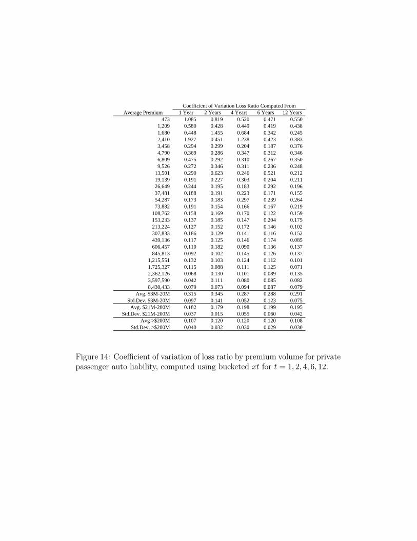
Coefficient of Variation Loss Ratio Computed From1 Year 2 Years 4 Years 6 Years 12 Years
473 1.085 0.819 0.520 0.471 0.5501,209 0.580 0.428 0.449 0.419 0.4381,680 0.448 1.455 0.684 0.342 0.2452,410 1.927 0.451 1.238 0.423 0.3833,458 0.294 0.299 0.204 0.187 0.3764,790 0.369 0.286 0.347 0.312 0.3466,809 0.475 0.292 0.310 0.267 0.3509,526 0.272 0.346 0.311 0.236 0.248
13,501 0.290 0.623 0.246 0.521 0.21219,139 0.191 0.227 0.303 0.204 0.21126,649 0.244 0.195 0.183 0.292 0.19637,481 0.188 0.191 0.223 0.171 0.15554,287 0.173 0.183 0.297 0.239 0.26473,882 0.191 0.154 0.166 0.167 0.219
108,762 0.158 0.169 0.170 0.122 0.159153,233 0.137 0.185 0.147 0.204 0.175213,224 0.127 0.152 0.172 0.146 0.102307,833 0.186 0.129 0.141 0.116 0.152439,136 0.117 0.125 0.146 0.174 0.085606,457 0.110 0.182 0.090 0.136 0.137845,813 0.092 0.102 0.145 0.126 0.137
1,215,551 0.132 0.103 0.124 0.112 0.1011,725,327 0.115 0.088 0.111 0.125 0.0712,362,126 0.068 0.130 0.101 0.089 0.1353,597,590 0.042 0.111 0.080 0.085 0.0828,430,433 0.079 0.073 0.094 0.087 0.079
Avg. $3M-20M 0.315 0.345 0.287 0.288 0.291Std.Dev. $3M-20M 0.097 0.141 0.052 0.123 0.075
Avg. $21M-200M 0.182 0.179 0.198 0.199 0.195Std.Dev. $21M-200M 0.037 0.015 0.055 0.060 0.042
Avg >$200M 0.107 0.120 0.120 0.120 0.108Std.Dev. >$200M 0.040 0.032 0.030 0.029 0.030
Average Premium
Figure 14: Coefficient of variation of loss ratio by premium volume for privatepassenger auto liability, computed using bucketed xt for t = 1, 2, 4, 6, 12.

Homeowners
0
0.20
0.40
0.60
0.80
1.00
1.20
1.40
1.60
1.80
2.00
100 1,000 10,000 100,000 1,000,000 10,000,000
Fit CVLR
0
0.20
0.40
0.60
0.80
1.00
1.20
1.40
1.60
1.80
2.00
100 1,000 10,000 100,000 1,000,000 10,000,000
CV CV2 CV4 CV6 CV12 Fit
Private Passenger Auto
0
0.20
0.40
0.60
0.80
1.00
1.20
1.40
1.60
1.80
2.00
100 1,000 10,000 100,000 1,000,000 10,000,000
Fit CVLR
0
0.20
0.40
0.60
0.80
1.00
1.20
1.40
1.60
1.80
2.00
100 1,000 10,000 100,000 1,000,000 10,000,000
CV CV2 CV4 CV6 CV12 Fit
Commercial Auto
0
0.20
0.40
0.60
0.80
1.00
1.20
1.40
1.60
1.80
2.00
100 1,000 10,000 100,000 1,000,000 10,000,000
Fit CVLR
0
0.20
0.40
0.60
0.80
1.00
1.20
1.40
1.60
1.80
2.00
100 1,000 10,000 100,000 1,000,000 10,000,000
CV CV2 CV4 CV6 CV12 Fit
Figure 15: Fit of
√σ2
xt + c to volatility by volume, xt, for homeowners,
private passenger auto and commercial auto. Left hand plot shows databased on a single year t = 1; right hand plot shows the same data for t =1, 2, 4, 6, 12.

Workers Compensation
0
0.20
0.40
0.60
0.80
1.00
1.20
1.40
1.60
1.80
2.00
100 1,000 10,000 100,000 1,000,000 10,000,000
Fit CVLR
0
0.20
0.40
0.60
0.80
1.00
1.20
1.40
1.60
1.80
2.00
100 1,000 10,000 100,000 1,000,000 10,000,000
CV CV2 CV4 CV6 CV12 Fit
Commercial Multiperil
0
0.20
0.40
0.60
0.80
1.00
1.20
1.40
1.60
1.80
2.00
100 1,000 10,000 100,000 1,000,000 10,000,000
Fit CVLR
0
0.20
0.40
0.60
0.80
1.00
1.20
1.40
1.60
1.80
2.00
100 1,000 10,000 100,000 1,000,000 10,000,000
CV CV2 CV4 CV6 CV12 Fit
Other Liability Occurrence
0
0.20
0.40
0.60
0.80
1.00
1.20
1.40
1.60
1.80
2.00
100 1,000 10,000 100,000 1,000,000 10,000,000
Fit CVLR
0
0.20
0.40
0.60
0.80
1.00
1.20
1.40
1.60
1.80
2.00
100 1,000 10,000 100,000 1,000,000 10,000,000
CV CV2 CV4 CV6 CV12 Fit
Figure 16: Fit of
√σ2
xt + c to volatility by volume, xt, for workers compen-
sation, commercial multiperil and other liability occurrence. Left hand plotshows data based on a single year t = 1; right hand plot shows the same datafor t = 1, 2, 4, 6, 12.

Actuarial Geometry
Finally, Figures 15 and 16 provide a graphical representation of the same
data for homeowners, private passenger auto, commercial auto, workers’ com-
pensation, commercial multi-peril and other liability occurrence (other lia-
bility claims made and medical malpractice lack the necessary volume). The
left hand plot shows the same data as Figure 5 on a log/linear scale and a
fit of υ(x, t) by√
(σ2/xt) + c. In the fit, c is estimated from the observed
asymptotic volatility and σ is estimated using minimum squared distance.
The right hand plot overlays υ(x/t, t) for t = 2, 4, 6, 12 using the method
described above. Thus the private passenger auto liability plot shows the
data in Figure 14. These plots support the hypothesis that υ(x/t, t) is inde-
pendent of t as there is no clear trend with t. (The case t = 12 is subject to
higher estimation error owing to the lower number of observations.)
We conclude that only model IM2 of IM1-4 and AM1 has volumetric and
temporal properties consistent with the data in the NAIC annual statement
database.
8 OPTIMIZATION AND HOMOGENEITY
This section sets up an explicit optimization problem which has a non-trivial
solution if and only if losses are homogeneous, A(x, t) = xX(t). It is the op-
timization derived by Myers and Read (2001), who also assume homogeneous
losses. The example is used to show how the homogeneity assumption leads
to a peculiar solution. We assume that t = 1 and drop t from the notation.
Assume there are n lines of business with loss processes Xi(x), E(Xi(x)) =
x. The loss processes are not assumed to be homogeneous. Assume there are
no expenses. The profit margin in line i is πi, so premium is (1+πi)xi. Capital
is denoted y. The cost of capital in excess of the risk free rate for insurance
capital is ν. The product market determines πi and the capital markets
determine ν. The company takes these variables as given. Assume that we
have a risk measure ρ : Rn × R → R where ρ(x1, . . . , xn, α) determines the
amount of capital corresponding to a safety level α ≥ 0. Using the implicit
function theorem gives a function α : Rn+1 → R so that
ρ(x1, . . . , xn, α(x1, . . . , xn, y)) = y. (59)
60

Actuarial Geometry
Consider the optimization problem of minimizing α subject to the cost
of capital constraint:minx1,...,xn,y α(x1, . . . , xn, y) subject to
∑i πixi = νy.
(60)
This problem is easy to solve using Lagrangian multipliers. The Lagrangian
is
L = α(x1, . . . , xn, y)− λ(∑
i
πixi − νy). (61)
Differentiating with respect to xi and y gives
∂L
∂xi
=∂α
∂xi
− λπi = 0 (62)
∂L
∂y=
∂α
∂y+ λν = 0. (63)
Thus, at the optimal solution
λ = − ∂α
∂xi
/πi =∂α
∂y/ν. (64)
Using the implicit function theorem gives
πi
ν=
∂y
∂xi
=∂ρ
∂xi
(65)
since y = ρ(x). Once again, at the optimal volume and capital levels, pricing
is proportional to the gradient vector. All optimization problems have a dual
which swaps the constraint and objective. Here, the dual problem maximizes
the return over cost of capital subject to a constraint on α. The dual can
be used to compute implied margins by line assuming the existing book of
business x1, . . . , xn and level of capital y are optimal. Again the margins are
proportional to the gradient vector.
Substituting Eq. 65 into the cost of capital constraint Eq. 60 gives
νy =∑
i
πixi =∑
i
νxi∂y
∂xi
(66)
61

Actuarial Geometry
and so
y =∑
i
xi∂y
∂xi
, (67)
recovering the Myers-Read adds-up result.
Mildenhall (2004) shows that Eq. 67 holds if and only if the loss pro-
cesses are homogeneous: Xi(x) = xXi. The above derivation appears to have
proved the same result without assuming homogeneity. The wrinkle is that
unless losses are homogeneous the solution is trivial: α = 0 and write no
business. It is clear this is always a solution of the optimization. The reason
there are other non-trivial solutions in the homogeneous case is the lack of
diversification. If Xi(x) diversifies then another solution to the optimization
involves growing infinitely large.
This is illustrated in Figure 17 when n = 2. Each plot shows volume x1, x2
in lines 1 and 2 in the horizontal plane and required capital ρ(x1, x2, α) at
a particular α level on the vertical axis. The flat green surface is a budget
constraint given by the cost of capital, π1x1 + π2x2 = νy. The left hand plot
shows diversifying insurance losses. The diversification effect can be seen
along the planes x1 = 0 and x2 = 0, which the capital surface intersects in a
concave down line. The Lagrangian requirement for a solution is that the flat
green plane be tangent to the capital surface. Since the surface is concave
down (reflecting diversification with volume in each line and diversification
between the two lines) the only possible tangent point with a plane through
the origin—such as the budget constraint—is the origin 0.12 The right hand
plot corresponds to a homogeneous model. The surface is “ruled”: it is
straight along rays from the origin rather than concave down. Now it is
possible for the budget plane to be tangent to the capital surface along an
entire line, including the origin. Such a line is illustrated on the plot. The
12If we use Lagrangian multipliers to maximize the difference∑
i πixi − νy at a givenα then the plane no longer goes through the origin. In this case there will be a uniquesolution in the diversifying case, but it will be a minimum and not a maximum. If X1 andX2 are correlated it is possible for the surface to be flat or convex along lines of the formx1+x2 = constant, but it will always be concave along rays from the origin for diversifyinginsurance losses.
62

Figure 17: Diversifying, inhomogeneous (left) and non-diversifying, homo-geneous (right) capital surfaces. The axes x1 and x2 represent the volumein each line and y represents capital at a fixed safety level α. The left plotwas produced assuming that Xi(x) = x +
√xZi for Zi independent standard
normal variables, and the right that Xi(x) = x + xZi. Thus Var(Xi(x)) = xon the left and Var(Xi(x)) = x2 on the right. This model can be extendedto model losses as x +
√xZ1 + xZ2 to produce an example with behavior
similar to IM2-4. It is tractable enough to have a closed form solution andyet varied enough to model all the different types of behavior of interest.

Actuarial Geometry
Myers-Read solution corresponds to a line of solutions along the ruled-capital
plane.
Some have tried to salvage Myers-Read’s adds-up result by arguing that
aggregate losses are “approximately homogeneous”. However, inhomogeneity
is material in realistically sized portfolios, Mildenhall (2004). The approx-
imation argument fails because Euler’s theorem uses derivatives and hence
requires a first order approximation rather than just pointwise equality. This
failure is supported by Figure 5 and is also illustrated in Figure 1 where k
and m cross at an angle. The fact that k(1) = m(1) does not guarantee
k′(1) = m′(1). Capital allocation and profit targets are usually set for seg-
ments of business generating $10-100M of premium. It is clear from Figure
5 that the volatility of losses decreases materially in this range—resulting in
a change in the geometry of the aggregate loss process—and invalidating the
adds-up result.
9 CONCLUSIONS
This paper provides an introduction to the actuarial use of Levy processes
to model aggregate losses. The Levy process model, reflecting the realities
of insurance, is an abelian convolution semigroup that is curved in both the
volume and time dimensions. Asset returns, in contrast, naturally form a real
vector space with scalar asset weights and are volumetrically flat. The paper
describes the relationship between Levy processes and catastrophe model
output. It clarifies the notion of a “direction” in the space of risks and uses
it to explain two different allocation results derived using the gradient of a
risk measure.
NAIC annual statement data is used to demonstrate that insurance li-
abilities do not diversify volumetrically or temporally. This paper reviews
four models of aggregate losses based on Levy processes—models with a long
risk-theoretic pedigree, it should be noted—and shows that only model IM2
is consistent with the NAIC data. It also shows how parameter risk can
64

Actuarial Geometry
be quantified at a distributional level. Volume-related parameter risk, ad-
justed for company and pricing cycle effects, is shown to have a Laplace
distribution—a surprising result.
In conclusion, this paper is a call-to-arms. Finance now provides a theo-
retical justification for pricing company-specific risk. Risk theory provides a
rigorous approach to evaluating and attributing risk to line using risk mea-
sure gradients. Enterprise Risk Management, which depends crucially on
an accurate quantification of aggregate loss distributions, demands accurate
and realistic modeling. It is time to satisfy that demand with a fully data-
grounded model for losses, including appropriate parameter risk.
References
Abraham, R., Marsden, J. E., and Ratiu, T. (1988). Manifolds, Tensor
Analysis, and Applications. Springer Verlag, second edition.
Applebaum, D. (2004). Levy Processes and Stochastic Calculus. Cambridge
University Press.
Artzner, P., Delbaen, F., Eber, J.-M., and Heath, D. (1999). Coherent mea-
sures of risk. Math. Finance, pages 203–28.
Bailey, R. A. (1967). Underwriting profits from investments. Proceedings of
the Casualty Actuarial Society, LIV:1–8.
Barndorff-Nielsen, O. E., Mikosch, T., and Resnick, S. I. (2001). Levy Pro-
ceeses - theory and applications. Birkhauser.
Beard, R. E., Pentikainen, T., and Pesonen, E. (1969). Risk Theory—The
Stochastic Basis of Insurance. Chapman and Hall, third edition.
Bertoin, J. (1996). Levy Processes. Cambridge University Press.
Borch, K. (1962). Equilibrium in a reinsurance market. Econometrica,
30(3):424–444.
65
Actuarial Geometry
Bowers, N., Gerber, H., Hickman, J., Jones, D., and Nesbitt, C. (1986).
Actuarial Mathematics. Society of Actuaries.
Breiman, L. (1992). Probability. Classics in Applied Mathematics. SIAM.
Buhlmann, H. (1970). Mathematical Models in Risk Theory. Springer Verlag.
Cheridito, P., Delbaen, F., and Kupper, M. (2003). Coherent and convex
risk measures for bounded cadlag processes. preprint.
Cummins, J. D. (1988). Risk-based premiums for insurance guarantee funds.
Journal of Finance, 43:823–839.
Cummins, J. D. and Geman, H. (1995). Pricing catastrophe insurance futures
and call spreads: An arbitrage approach. J. of Fixed Income, 4(4):46–57.
Cummins, J. D. and Harrington, S. A. (1987). Fair Rate of Return in
Property-Liability Insurance. Kluwer-Nijhoff.
Cummins, J. D. and Phillips, R. D. (2000). Applications of financial pricing
models in property-liability insurance. In Dionne, G., editor, Handbook of
Insurance. Kluwer Academic.
D’Arcy, S. and Dyer, M. A. (1997). Ratemaking: A financial economics
approach. Proceedings of the Casualty Actuarial Society, LXXXIV:301–
390.
D’Arcy, S. P. and Doherty, N. A. (1988). The Financial Theory of Pric-
ing Property Liability Insurance Contracts. Huebner Foundation/Irwin,
Homewood IL.
Daykin, C. D., Pentikainen, T., and Pesonen, M. (1994). Practical Risk
Theory for Actuaries. Chapman and Hall.
Delbaen, F. (2000a). Coherent risk measures. Monograph, Scoula Normale
Superiore.
66

Actuarial Geometry
Delbaen, F. (2000b). Coherent risk measures on general probability spaces.
In Essays in Honour of Dieter Sondermann. Springer Verlag.
Delbaen, F. and Haezendonck, J. (1989). A martingale approach to premium
calculation principles in an arbitrage free market. Insurance: Mathematics
and Economics, 8:269–277.
Denault, M. (2001). Coherent allocation of risk capital. preprint.
Doherty, N. A. and Garven, J. R. (1986). Price regulation in property-
liability insurance: A contingent claims approach. Journal of Finance,
XLI(5):1031–1050.
Feller, W. (1971). An Introduction to Probability Theory and Its Applications,
two volumes. J. Wiley and Sons, second edition.
Ferrari, J. R. (1968). The relationship of underwriting, investment, leverage,
and exposure to total return on owners’ equity. Proceedings of the Casualty
Actuarial Society, LV:295–302.
Fischer, T. (2003). Risk capital allocation by coherent risk measures based on
one-sided moments. Insurance: Mathematics and Economics, 32:135–146.
Follmer, H. and Schied, A. (2002). Convex measures of risk and trading
constraints. Finance and Stochastics, 6(4).
Froot, K. A. (2003). Risk management, capital budgeting and capital struc-
ture policy for insurers and reinsurers. NBER Working Paper Series,
10184.
Froot, K. A., Scharfstein, D. S., and Stein, J. C. (1993). Risk management:
Coordinating corporate investment and financing policies. Journal of Fi-
nance, XLVIII (5):1629–1658.
Froot, K. A. and Stein, J. C. (1998). Risk management, capital budget-
ing, and capital structure policy for inancial institutions: an integrated
approach. Journal of Financial Economics, 47:52–82.
67

Actuarial Geometry
Goovaerts, M. J., de Vylder, F., and Haezendonck, J. (1984). Insurance
Premiums. North-Holland.
Hull, J. C. (1983). Options Futures and Other Derivative Securities. Prentice-
Hall, second edition.
Kalkbrener, M. (2005). An axiomatic approach to capital allocation. Math-
ematical Finance, to appear.
Kallop, R. H. (1975). A current look at workers’ compensation ratemaking.
Proceedings of the Casualty Actuarial Society, LXII:62–81.
Karatzas, I. and Shreve, S. (1988). Brownian Motion and Stochastic Calculus.
Springer-Verlag, New York.
Klugman, S. A., Panjer, H. H., and Willmot, G. E. (1998). Loss Models,
From Data to Decisions. John Wiley and Sons.
Kotz, S., Kozubowski, T., and Podgorski, K. (2001). The Laplace Distribu-
tion and Generalizations. Birkhauser.
Lange, J. T. (1966). General liability insurance ratemaking. Proceedings of
the Casualty Actuarial Society, LIII:26–53.
Magrath, J. J. (1958). Ratemaking for fire insurance. Proceedings of the
Casualty Actuarial Society, XLV:176–195.
McGuinness, J. S. (1969). Is “probable maximal loss” (PML) a useful con-
cept? Proceedings of the Casualty Actuarial Society, LVI:31–40.
Meister, S. (1995). Contributions to the mathematics of catastrophe insur-
ance futures. ETH.
Merton, R. C. and Perold, A. (2001). Theory of risk capital in financial
firms. In Donald H. Chew, J., editor, The New Corporate Finance, Where
Theory Meets Practice, pages 438–454. McGraw-Hill.
68

Actuarial Geometry
Meyers, G. (2003). The economics of capital allocation. preprint.
http://www.aria.org/rts/rts2005/proceedings05.htm.
Meyers, G. (2005a). The common shock model for correlated insurance losses.
Proceedings of the Risk Theory Society.
Meyers, G. (2005b). Distributing capital: Another tactic. The Actuarial
Review, November:25–26. with on-line technical appendix.
Mildenhall, S. (2004). A note on the Myers and Read capital allocation
formula. North American Actuarial Journal, 8(2):32–44.
Miller, R. B. and Wichern, D. W. (1977). Intermediate Business Statistics:
Analysis of Variance, Regression and Time Series. HRW.
Myers, S. C. and Read, J. A. (2001). Capital allocation for insurance com-
panies. Journal of Risk and Insurance, 68 no. 4:545–580.
Panjer, H. H. (2001). Measurement of risk, solvency requirements and allo-
cation of capital within financial congolomerates. preprint.
Panjer, H. H. and Willmot, G. E. (1992). Insurance Risk Models. Society of
Actuaries.
Perold, A. F. (2001). Capital allocation in financial firms. HBS Competition
and Strategy Working Paper Series, 98-072.
Phillips, R. D., Cummins, J. D., and Allen, F. (1998). Financial pricing of
insurance in the multiple-line insurance company. The Journal of Risk and
Insurance, 65(4):597–636.
Ravishanker, N. and Dey, D. K. (2002). A First Course in Linear Model
Theory. Chapman & Hall/CRC.
Sato, K.-I. (1999). Levy Processes and Infinitely Divisible Distributions. Cam-
bridge University Press.
69
Actuarial Geometry
Sherris, M. (2006). Solvency, capital allocation and fair rate of return in
insurance. Journal of Risk and Insurance, 73(1):71–96.
Stroock, D. W. (1993). Probability Theory, An Analytic View. Cambridge
University Press.
Stroock, D. W. (2003). Markov Processes from K. Ito’s Perspective. Annals
of Mathematics Studies. Princeton University Press.
Tasche, D. (2000). Risk contributions and performance measurement.
preprint.
Zanjani, G. (2002). Pricing and capital allocation in catastrophe insurance.
Journal of Financial Economics, 65:283–305.
Biography of the AuthorStephen Mildenhall is an Executive Vice President at Aon Re Services in
Chicago Illinois. Aon Re Services is the technical arm of Aon Re, the world’slargest reinsurance intermediary. At Aon Re, Stephen heads a team of actuariesproviding a variety of actuarial services for clients, including reinsurance pricingand structure evaluation, dynamic financial analysis, capital allocation and pre-dictive modeling. Prior to joining Aon Re, Stephen worked at Kemper Insuranceand CNA Insurance. He has an undergraduate degree in Mathematics from theUniversity of Warwick, England, and a Masters and Doctorate in Mathematicsfrom the University of Chicago. Stephen is a Fellow of the Casualty ActuarialSociety, an Associate of the Society of Actuaries and a Member of the AmericanAcademy of Actuaries. His research interests include risk theory, capital determi-nation, allocation and optimization, and applications of statistics to reserving andratemaking problems.
70