actuator cylinder theory for multiple vertical axis … cylinder theory for multiple vertical axis...

Wind Energ. Sci., 1, 327–340, 2016www.wind-energ-sci.net/1/327/2016/doi:10.5194/wes-1-327-2016© Author(s) 2016. CC Attribution 3.0 License.

Actuator cylinder theory for multiplevertical axis wind turbines

Andrew NingBrigham Young University, Provo, UT, USA

Correspondence to: Andrew Ning ([email protected])

Received: 13 May 2016 – Published in Wind Energ. Sci. Discuss.: 31 May 2016Revised: 15 September 2016 – Accepted: 7 November 2016 – Published: 16 December 2016

Abstract. Actuator cylinder theory is an effective approach for analyzing the aerodynamic performance ofvertical axis wind turbines at a conceptual design level. Existing actuator cylinder theory can analyze singleturbines, but analysis of multiple turbines is often desirable because turbines may operate in near proximitywithin a wind farm. For vertical axis wind turbines, which tend to operate in closer proximity than do horizontalaxis turbines, aerodynamic interactions may not be strictly confined to wake interactions. We modified actuatorcylinder theory to permit the simultaneous solution of aerodynamic loading for any number of turbines. Wealso extended the theory to handle thrust coefficients outside of the momentum region and explicitly defined theadditional terms needed for curved or swept blades.

While the focus of this paper is a derivation of an extended methodology, an application of this theory wasexplored involving two turbines operating in close proximity. Comparisons were made against two-dimensionalunsteady Reynolds-averaged Navier–Stokes (URANS) simulations, across a full 360◦ of inflow, with excellentagreement. The counter-rotating turbines produced a 5–10 % increase in power across a wide range of inflowconditions. A second comparison was made to a three-dimensional RANS simulation with a different turbineunder different conditions. While only one data point was available, the agreement was reasonable, with thecomputational fluid dynamics (CFD) predicting a 12 % power loss, as compared to a 15 % power loss for the ac-tuator cylinder method. This extended theory appears promising for conceptual design studies of closely spacedvertical axis wind turbines (VAWTs), but further development and validation is needed.

1 Introduction

Blade element momentum theory combines momentum the-ory across an actuator disk with blade element theory to pre-dict the aerodynamic loading of horizontal axis wind turbines(HAWTs). This theory has been very successful and is heav-ily used in many analysis and design applications (Hansen,2008; Manwell et al., 2009; Burton et al., 2011; Ning, 2014).Its primary advantage is computational speed while still pro-viding reasonably accurate performance predictions.

Streamtube theory attempts to apply the same conceptto vertical axis wind turbine (VAWT) aerodynamic perfor-mance estimation (Templin, 1974). Each cross section ofthe VAWT (constant height) is approximated as an actua-tor disk through the mid-plane, which results in a cross-plane actuator line in the 2-D plane. However, this model is

a rather poor representation of a VAWT as it requires con-stant flow parameters across the entire disk. An extensionof this theory is multiple streamtube theory, where, insteadof using one large streamtube passing through the VAWT,the VAWT cross section is discretized into multiple stream-tubes each with an independent induction factor (Wilsonand Lissaman, 1974; Strickland, 1975). An additional exten-sion, double multiple streamtube theory (Paraschivoiu, 1981,1988; Paraschivoiu and Delclaux, 1983), utilizes two actua-tor disks to represent the upstream and downstream sides ofthe cylinder (Fig. 1). In this model, momentum losses can oc-cur on both the upwind and downwind faces. Double multi-ple streamtube theory has been widely used for aerodynamicanalysis of VAWTs.

Published by Copernicus Publications on behalf of the European Academy of Wind Energy e.V.

328 A. Ning: Multiple VAWT AC theory

V V 0

V1

Figure 1. Double multiple streamtube concept with multiplestreamtubes along the VAWT (one shown) and separate “actuatordisks” on both the upstream and downstream surfaces.

While double multiple streamtube theory is a useful im-provement over single streamtube models, it is clearly aforced application of the actuator disk concept to a VAWT.A more physically consistent theory for VAWTs, called ac-tuator cylinder theory, was developed by Madsen (Madsen,1982; Madsen et al., 2013). Actuator cylinder theory hasbeen shown to be more accurate than double multiple stream-tube theory (Ferreira et al., 2014), while still retaining com-parable computational speed.

One limitation of actuator cylinder theory is that it is de-rived only for a single isolated turbine. We are interested inperformance of VAWT farms and thus need to predict perfor-mance of multiple VAWTs in proximity to each other. Thispaper extends the methodology for use with any number ofVAWTs, extends applicability to turbines not operating in themomentum region, and adds computation details for bladesthat are curved or swept. The primary purpose of this paperis to derive the new methodology, but some example tradestudies of VAWT pairs are also discussed.

2 Theory development

The actuator cylinder theory begins with the assumptionthat a vertical slice of a VAWT can be modeled as a two-dimensional problem. Figure 2 shows a 2-D representationof the VAWT, with only one of the blades shown for simplic-ity, and defines the coordinate system used in this derivation.The VAWT produces a varying normalized radial force perunit length q(θ ) as a function of azimuthal position alongthe VAWT. We define the positive direction for this forceq as positive radial outward (and thus positive radially in-ward for the loads the fluid produces on the VAWT). Us-ing the two-dimensional, steady, incompressible, Euler equa-tions, and (for the moment) neglecting nonlinear terms, theinduced velocities at any location in the plane can be shownto be given by the following integrals (Madsen et al., 2013;Madsen, 1982):

u(x,y)=1

2π

2π∫0

q(θ )[x+ sinθ ] sinθ −

[y− cosθ

]cosθ

[x+ sinθ ]2+[y− cosθ

]2 dθ

✓

x

y

V1

q(✓)

Figure 2. A canonical 2-D slice of a VAWT (only one blade shown)and the coordinate system used.

✓y

Integration path

Figure 3. Integration path for a point inside the cylinder.

− q(

cos−1y){inside and wake}

+ q(−cos−1y

){wake only}

v(x,y)=1

2π

2π∫0

q(θ )[x+ sinθ ]cosθ +

[y− cosθ

]sinθ

[x+ sinθ ]2+[y− cosθ

]2 dθ,

(1)

where the x, y position is measured from the center of aunit radius turbine, and velocities are normalized by thefreestream velocity. For evaluation points inside the cylin-der the {inside and wake} term applies, and for evaluationpoints downstream of the cylinder both the {inside and wake}and {wake only} terms apply. These two terms are based onan integration path through the cylinder, where θ = cos−1y

(Fig. 3). For brevity, the derivations of the above equationsare omitted, but details are available in the above-cited pa-pers from Madsen.

These two equations for the induced velocities (Eq. 1) areapplicable for any x, y location; however, we are primarilyinterested in the induced velocities only at locations on thecurrent turbine and on other turbines. To facilitate computa-tion we discretize the description of each actuator cylinder

Wind Energ. Sci., 1, 327–340, 2016 www.wind-energ-sci.net/1/327/2016/

A. Ning: Multiple VAWT AC theory 329

into n panels centered at the azimuthal locations:

θi = (2i− 1)π

nfor i = 1. . .n,

1θ =2πn. (2)

Furthermore, as is done in the original version, we assumepiecewise constant loading across each panel. These loca-tions are the points of interest where will compute the radialforces and subsequently the induced velocities.

In general, we need to compute the induced velocity atevery location on a given VAWT using contributions fromall VAWTs (including itself). In the following derivation weadopt the notation that index I is the turbine we are evalu-ating the velocities at, and index i represents the azimuthallocation on turbine I where we are evaluating. Index J willrefer to the turbine producing the induced velocity, and indexj will indicate the azimuthal location on turbine J where theload is producing the induced velocity (Fig. 4).

Using the azimuthal discretization, the induced velocitiesat a point (x,y) are expressed as a sum of integrals over indi-vidual panels. Recall that Eq. (1) is normalized based on thecurrent VAWT radius and the freestream velocity. Becausewe are now considering multiple VAWTs with potentiallydifferent radii, we need to be more explicit in defining thenormalized quantities. The generalized definitions of the x,yevaluation positions are

x∗i =(xi − xJc

)/rJ ,

y∗i =(yi − yJc

)/rJ , (3)

where xJc is the x location of the center of turbine J . If I = J(i.e., we are evaluating the turbine’s influence on itself), thenthis definition is identical to the single-turbine case where thex and y locations are then distances from the VAWT centernormalized by its radius.

The velocity used in normalizing the induced velocitiesand the radial loading must be the same, and for that pur-pose we continue to use the freestream velocity. We intro-duce the asterisk superscript on the induced velocities forclarity (e.g., u∗ = u/V∞). The expressions for induced ve-locity at the cylinder surface depend on whether we evaluatejust upstream of the actuator disk or just downstream. Theend result is the same, as long as we are consistent. In thefollowing derivation we evaluate on the upstream surfacesfor both halves of the actuator disk.

u∗i =1

2π

∑j

qj

θj+1θ/2∫θj−1θ/2

(x∗i + sinφ) sinφ− (y∗i − cosφ)cosφ(x∗i + sinφ)2+ (y∗i − cosφ)2 dφ

− qn+1−i {I = J, i > n/2}

− qJk + qJn+1−k {I 6= J, −1≤ y∗i ≤ 1, x∗i ≥ 1}

I

J

i

j

ui

vi

qj

✓j

Figure 4. Influence of load at location j of turbine J onto locationi of turbine I .

(where index k satisfies θJk = cos−1y∗i

)v∗i =

12π

∑j

qj


(x∗i + sinφ)cosφ+ (y∗i − cosφ) sinφ(x∗i + sinφ)2+ (y∗i − cosφ)2 dφ (4)

In these integrals we have replaced θ in the integration withthe dummy variable φ in order to avoid confusion with the θterms appearing in the integration limits. The term −qn+1−iarises when evaluating the influence of a turbine on itself. Be-cause we chose to evaluate on the upstream surfaces, the up-stream half of the VAWT is considered outside of the VAWT,but the aft half is in the inside of the cylinder. This impliesthat for the aft half (i.e., i > n/2) the −q(cos−1y) term mustbe added. This corresponds to the loading on the front half ofthe turbine with the same y value. Based on our discretiza-tion, its location can be indexed directly as −qn+1−i .

The following two terms for u arise when turbine I is inthe wake of turbine J . Actuator cylinder theory only includesthe wake term when an evaluation point is directly down-wind from a source point (e.g., the blue region in Fig. 5).The condition corresponds to x∗i ≥ 1 and −1≤ y∗i ≤ 1 andx∗i

2+ y∗i

2≥ 1. For this wake area, both of the terms in Eq. 1

are applicable. The index k corresponds to the location whereθJk = cos−1y∗i . Note that cos−1y∗i will likely not line up ex-actly with an existing grid point θk on turbine J , but we haveassumed piecewise constant loading across a given panel, sok will correspond to the panel that is intersected.

This model is based on integration paths like those shownin Fig. 3 and thus ignores the effect of wake expansion andviscous decay. An alternative is to ignore the wake termsand instead apply a momentum deficit factor from someother VAWT wake model. For example, we have developed areduced-order wake model based on computational fluid dy-namics (CFD) simulations that predicts the velocity deficitbehind a VAWT (Tingey and Ning, 2016). Rather than use

www.wind-energ-sci.net/1/327/2016/ Wind Energ. Sci., 1, 327–340, 2016


J

Figure 5. Wake region from actuator cylinder theory highlighted inblue (and extending downstream).

the above wake terms, one could use the separate wake modelto evaluate the velocity deficit at each control point and sub-tract the deficit from u∗. Because the focus on this paper is onactuator cylinder theory, we will use the simple wake modelthat naturally arises within the theory itself, but this method-ology provides a convenient hook to insert any wake model.

For convenience in the computation, Eq. (4) can be ex-pressed as a matrix vector multiplication where the loadingq is separated from the influence coefficients.

u∗I = AxI J qJv∗I = AyI J qJ (5)

The matrix AyI J is given by

AyI J (i,j )=1

2π


(x∗i + sinφ)cosφ+ (y∗i − cosφ) sinφ(x∗i + sinφ)2+ (y∗i − cosφ)2 dφ. (6)

For the AxI J matrix we divide the contributions betweenthe direct influence and the wake influence: AxI J = DxI J +WxI J , where

DxI J (i,j )=1

2π


(x∗i + sinφ) sinφ− (y∗i − cosφ)cosφ(x∗i + sinφ)2+ (y∗i − cosφ)2 dφ, (7)

WxI J (i,j )=

−1 if − 1≤ y∗i ≤ 1 and x∗i ≥ 0and x∗i

2+ y∗i

2≥ 1 and j = k

1 if − 1≤ y∗i ≤ 1 and x∗i ≥ 0and x∗i

2+ y∗i

2≥ 1

and j = n− k+ 10 otherwise,

(8)

where index k corresponds to the panel where θJk =

cos−1y∗i .If we are evaluating the influence of a turbine on itself

(e.g., I = J ) then the computations in the Ax matrix canbe simplified. We can expand using the definitions for x

and y along the cylinder (x∗i =−sinθi and y∗i = cosθi fori = 1. . .n). As long as i 6= j , then the integral in Eq. (7) eval-uates to 1θ/2. When i = j the value of the integral dependson which side of the cylinder we evaluate on. It convergesto π (−1+ 1/n) just outside of the cylinder and π (1+ 1/n)just inside. Because we chose to evaluate on the upstreamsurface on both halves of the cylinder, the integral evalu-ates to π (−1+1/n) on the upstream half of the cylinder andπ (1+ 1/n) on the downstream half of the cylinder.

DxI I (i,j )=

1θ/(4π ) if i 6= j(−1+ 1/n)/2 if i = j and i ≤ n/2(1+ 1/n)/2 if i = j and i > n/2

(9)

WxI I (i,j )={−1 if i > n/2 and j = n+ 1− i0 otherwise (10)

If a user elects to use a more sophisticated wake model theWx term can simply be ignored and a separate momentumdeficit factor can be applied.

2.1 Faster computation

The bulk of the computational effort is contained in comput-ing the influence coefficient matrices AxI J and AyI J . Thesecomputations consist of a double loop iterating across allevaluation positions i on turbine I for each source positionj on turbine J (which is itself contained in a double loopacross all turbines I and J ). Fortunately, some of this com-putation can be simplified. The expressions in Eqs. (6), (9),and (10) apply for the cases where I = J , or in other wordsfor computing the influence of the turbine on itself. A signif-icant benefit to this equation form is that the matrices dependonly on the discretization of the cylinder and not on the de-tails of the blade shape or loading. For a preselected numberof azimuthal segments (e.g., n= 36), these matrices can beprecomputed and stored. This is true no matter what size ra-dius the VAWT is.

If I 6= J , some reduction in computational requirementsis also possible. For each VAWT pair (I 6= J ), if the twoVAWTs are of equal radius, then pairs of influence coeffi-cients between them are exactly the same. As seen in Fig. 6,the distance vector from the center of one turbine to the eval-uation point on a separate turbine is exactly equal and oppo-site to a vector originating from the center of the other tur-bine and terminating at an azimuthal location diametricallyopposite to the first evaluation point’s azimuthal location. Aslong as these two VAWTs are of equal radius, these two vec-tors will always be equal and opposite. This corresponds tox∗ and y∗ switching signs in Eqs. (6) and (7). However, theevaluation locations are always 180◦ apart in location. Thiscorresponds to switching the sign on all sin and cos terms.The two sign changes cancel out and thus the two evalua-tion coefficients will be exactly the same. In other words, forall pairs of VAWTs that are of equal radii, only one set of



✓

⇡ + ✓

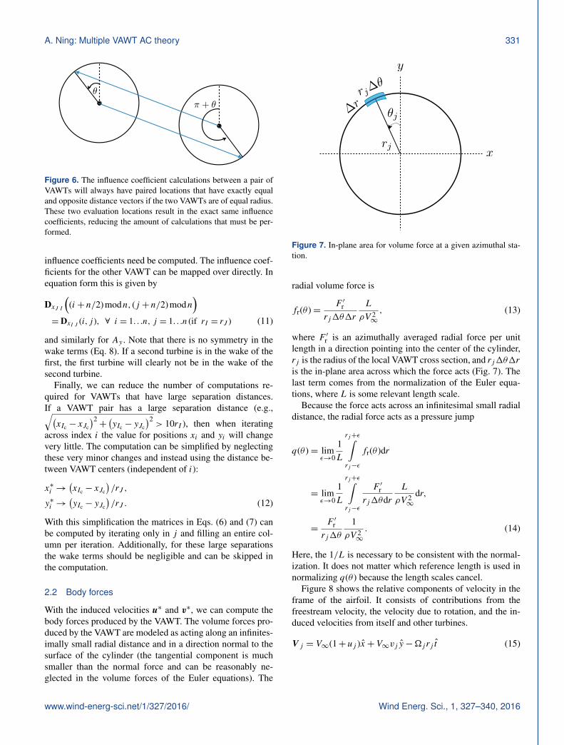
Figure 6. The influence coefficient calculations between a pair ofVAWTs will always have paired locations that have exactly equaland opposite distance vectors if the two VAWTs are of equal radius.These two evaluation locations result in the exact same influencecoefficients, reducing the amount of calculations that must be per-formed.

influence coefficients need be computed. The influence coef-ficients for the other VAWT can be mapped over directly. Inequation form this is given by

DxJ I(

(i+ n/2)modn, (j + n/2)modn)

= DxI J (i,j ), ∀ i = 1. . .n, j = 1. . .n (if rI = rJ ) (11)

and similarly for Ay . Note that there is no symmetry in thewake terms (Eq. 8). If a second turbine is in the wake of thefirst, the first turbine will clearly not be in the wake of thesecond turbine.

Finally, we can reduce the number of computations re-quired for VAWTs that have large separation distances.If a VAWT pair has a large separation distance (e.g.,√(xIc − xJc

)2+(yIc − yJc

)2> 10rI ), then when iterating

across index i the value for positions xi and yi will changevery little. The computation can be simplified by neglectingthese very minor changes and instead using the distance be-tween VAWT centers (independent of i):

x∗i →(xIc − xJc

)/rJ ,

y∗i →(yIc − yJc

)/rJ . (12)

With this simplification the matrices in Eqs. (6) and (7) canbe computed by iterating only in j and filling an entire col-umn per iteration. Additionally, for these large separationsthe wake terms should be negligible and can be skipped inthe computation.

2.2 Body forces

With the induced velocities u∗ and v∗, we can compute thebody forces produced by the VAWT. The volume forces pro-duced by the VAWT are modeled as acting along an infinites-imally small radial distance and in a direction normal to thesurface of the cylinder (the tangential component is muchsmaller than the normal force and can be reasonably ne-glected in the volume forces of the Euler equations). The

x

y

✓j�r

rj

rj�✓

Figure 7. In-plane area for volume force at a given azimuthal sta-tion.

radial volume force is

fr(θ )=F ′r

rj1θ1r

L

ρV 2∞

, (13)

where F ′r is an azimuthally averaged radial force per unitlength in a direction pointing into the center of the cylinder,rj is the radius of the local VAWT cross section, and rj1θ1ris the in-plane area across which the force acts (Fig. 7). Thelast term comes from the normalization of the Euler equa-tions, where L is some relevant length scale.

Because the force acts across an infinitesimal small radialdistance, the radial force acts as a pressure jump

q(θ )= limε→0

1L

rj+ε∫rj−ε

fr(θ )dr

= limε→0

1L

rj+ε∫rj−ε

F ′rrj1θdr

L

ρV 2∞

dr,

=F ′rrj1θ

1ρV 2∞

. (14)

Here, the 1/L is necessary to be consistent with the normal-ization. It does not matter which reference length is used innormalizing q(θ ) because the length scales cancel.

Figure 8 shows the relative components of velocity in theframe of the airfoil. It consists of contributions from thefreestream velocity, the velocity due to rotation, and the in-duced velocities from itself and other turbines.

V j = V∞(1+ uj )x+V∞vj y−�j rj t (15)



n

t

x

y

V1(1 + uj)

V1vj

✓j

⌦jrj

Figure 8. Relative components of velocity in the frame of the air-foil.

n

t

x

y

✓j

V1(1 + uj) sin ✓j � V1vj cos ✓j

V1(1 + uj) cos ✓j + V1vj sin ✓j + ⌦jrj

Figure 9. Components of velocity resolved into n− t plane.

Using the following coordinate transformations,

x =−cosθj t − sinθj n

y =−sinθj t + cosθj n, (16)

the velocity can be expressed in the n–t plane as

V j =[−V∞(1+ uj ) sinθj +V∞vj cosθj

]n

+[−V∞(1+ uj )cosθj −V∞vj sinθj −�j rj

]t . (17)

These velocity components are depicted in Fig. 9.If we define the magnitudes

Vnj ≡ V∞(1+ uj ) sinθ −V∞vj cosθ,

Vtj ≡ V∞(1+ uj )cosθ +V∞vj sinθ +�j rj , (18)

then

V j =−Vnj n−Vtj t (19)

and the magnitude of the local relative velocity and local in-flow angle (Fig. 10) are

Wj =

√V 2

nj +V2tj ,

W

� t

n

cn

ct

cl

cd

Figure 10. Definition of normal and tangential force coefficients.

φj = tan−1

(Vnj

Vtj

). (20)

The angle of attack, Reynolds number, and lift and drag co-efficients can then be estimated as

αj = φj −β

Rej =ρWj c

µ

clj = f (αj ,Rej )

cdj = f (αj ,Rej ). (21)

This can be rotated into normal and tangential force coef-ficients (note that cn is defined as positive in the oppositedirection of n in Fig. 10).

cnj = clj cosφj + cdj sinφjctj = clj sinφj − cdj cosφj (22)

We can resolve these normal and tangential loads into aradial, tangential, and vertical coordinate system. In doingso, we will account for blade curvature, as is often used withVAWTs, an example of which is shown in Fig. 11. The totalforce vector is resolved as

F =12ρW 2(−cnn+ ct t)1a, (23)

where the negative sign results from the coordinate systemdefinition seen in Fig. 10. From Fig. 11 we see that the areaof the blade element is

1a = c1s = c1z

cosδ, (24)

and the unit vector n can be expressed as

n= cosδr + sinδz. (25)

Thus, the force vector per unit depth (unit length in the z di-rection) is

F ′ =ρW 2c

2cosδ

(− cn cosδ r − cn sinδ z+ ct t

). (26)



n

r

z

�dz

ds =dz

cos �

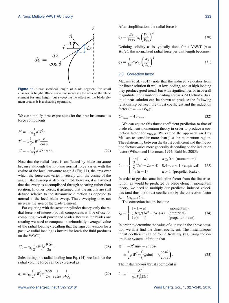
Figure 11. Cross-sectional length of blade segment for smallchanges in height. Blade curvature increases the area of the bladeelement for unit height, but sweep has no effect on the blade ele-ment area as it is a shearing operation.

We can simplify these expressions for the three instantaneousforce components:

R′ =−cn12ρW 2c

T ′ = ct12ρW 2 c

cosδ

Z′ =−cn12ρW 2c tanδ. (27)

Note that the radial force is unaffected by blade curvaturebecause although the in-plane normal force varies with thecosine of the local curvature angle δ (Fig. 11), the area overwhich the force acts varies inversely with the cosine of theangle. Blade sweep is also permitted; however, it is assumedthat the sweep is accomplished through shearing rather thanrotation. In other words, it assumed that the airfoils are stilldefined relative to the streamwise direction as opposed tonormal to the local blade sweep. Thus, sweeping does notincrease the area of the blade element.

For equating with the actuator cylinder theory, only the ra-dial force is of interest (but all components will be of use forcomputing overall power and loads). Because the blades arerotating we need to compute an azimuthally averaged valueof the radial loading (recalling that the sign convention for apositive radial loading is inward for loads the fluid produceson the VAWT):

F ′rj = cnj12ρW 2

j cB1θ

2π. (28)

Substituting this radial loading into Eq. (14), we find that theradial volume force can be expressed as

qj = cnj12ρW 2

j cB1θ

2π1

rj1θ

1ρV 2∞

. (29)

After simplification, the radial force is

qj =Bc

4πrjcnj

(Wj

V∞

)2

. (30)

Defining solidity as is typically done for a VAWT (σ =Bc/r), the normalized radial force per unit length becomes

qj =1

4πσj cnj

(Wj

V∞

)2

. (31)

2.3 Correction factor

Madsen et al. (2013) note that the induced velocities fromthe linear solution fit well at low loading, and at high loadingthey produce good trends but with significant error in overallmagnitude. For a uniform loading across a 2-D actuator disk,this linear solution can be shown to produce the followingrelationship between the thrust coefficient and the inductionfactor (a =−u/V∞):

CTlinear = 4alinear. (32)

We can equate this thrust coefficient prediction to that ofblade element momentum theory in order to produce a cor-rection factor for alinear. We extend the approach used byMadsen to consider more than just the momentum region.The relationship between the thrust coefficient and the induc-tion factors varies more generally depending on the inductionfactor (Wilson and Lissaman, 1974; Buhl Jr., 2005):

CT =

4a(1− a) a ≤ 0.4 (momentum)29

(7a2− 2a+ 4) 0.4< a < 1 (empirical)

4a(a− 1) a > 1 (propeller brake).

(33)

In order to get the same induction factor from the linear so-lution, as would be predicted by blade element momentumtheory, we need to multiply our predicted induced veloci-ties (and thus the thrust coefficient) by the correction factorka = CTlinear/CT.

The correction factors become

ka =

1/(1− a) (momentum)(18a)/(7a2

− 2a+ 4) (empirical)1/(a− 1) (propeller brake).

(34)

In order to determine the value of a to use in the above equa-tion we first find the thrust coefficient. The instantaneousthrust coefficient can be found from Eq. (27) using the co-ordinate system definition that

X′ =−R′ sinθ − T ′ cosθ

=12ρW 2c

(cn sinθ − ct

cosθcosδ

). (35)

The instantaneous thrust coefficient is

CTinst =X′

12ρV

2∞(2r)



=

(W

V∞

)2c

2r

(cn sinθ − ct

cosθcosδ

), (36)

where the other normalization dimension comes from the dis-tributed loads, which are a force per unit length in the z di-rection. To get the total thrust coefficient we need to computethe azimuthal average:

CT =B

2π

2π∫0

CTinst (θ )dθ

=σ

4π

2π∫0

(W

V∞

)2(cn sinθ − ct

cosθcosδ

)dθ. (37)

From the thrust coefficient we can compute the expected in-duction factor by reversing Eq. (33):

a =

12

(1−

√1−CT

)CT ≤ 0.96 (momentum)

17

(1+ 3

√72CT− 3

)0.96< CT < 2 (empirical)

12

(1+

√1+CT

)CT > 2 (propeller brake).

(38)

Finally, this induction factor allows us to compute the correc-tion factor from Eq. (34). These factors should be multipliedagainst the induced velocities, but because that is the quantitywe need to solve for, we must multiply against their predictedvalues.

Because this correction is derived for an isolated turbine,the correction factors k1. . .kN should be precomputed foreach individual turbine in isolation rather than as part of thecoupled solve of all turbines together.

2.4 Matrix assembly and solution procedure

From the proceeding discussion it should be noted that com-puting loads depends on the induced velocities, but comput-ing the induced velocities depends on the loads. Thus, an it-erative root-finding approach is required. We can assemblethe self-induction and mutual induction effects into one largematrix composed of block matrices. We also need to applythe various correction factors k for turbine J . To solve allinduced velocities as one large system we will concatenatethe u and v velocity vectors into one vector: w = [u;v]. Inthe equation below, the symbol � represents an element-by-element multiplication.

u1u2...

uN−−

v1v2...

vN

=

k1k2...

kN−−

k1k2...

kN

Figure 12. Example two-dimensional discretization in height andazimuthal position of swept surface (side view).

�

Ax Ax12 . . . Ax1NAx21 Ax . . . Ax2N...

.

.

.. . .

.

.

.AxN1 AxN2 . . . Ax−−−−− −−−−− −− −−−−−

Ay Ay12 . . . Ay1NAy21 Ay . . . Ay2N...

.

.

....

.

.

.AyN1 AyN2 . . . Ay

q1q2...

qN

(39)

We now have a matrix vector expression of the form w = Aq,but because q depends on w we must solve for w using aroot-finding method. The residual equation is

f (w)= Aq(w)−w = 0. (40)

Any good n-dimensional root finder can be used. This pa-per uses the modified Powell hybrid method as contained inhybrd.f of Minpack.

2.5 Variations in height

The actuator cylinder theory computes all loads in two-dimensional cross sections. We can use a representative sec-tion to represent the whole turbine (which is more appropri-ate for an H-Darrieus geometry, ignoring wind shear), or wecan additionally discretize the turbine along the height andcompute loads at each section.

For each azimuthal station of interest, the solution is pro-jected onto the instantaneous locations of the blade dis-cretization as shown in Fig. 12. For an unswept blade, thisinvolves just a straightforward transfer of forces as the bladediscretization would typically be exactly aligned with thesurface discretization. However, for swept blades, interpola-tion is necessary to resolve the forces along the curved bladepath. Furthermore, for a swept blade, the normal and tangen-tial directions change along the blade path. For swept blades,each point along the blade is at some azimuthal offset (1θ )from a reference point (e.g., relative to the equatorial bladelocation), and the total normal force, tangential force, andtorque produced by the blade are (again 1θ = 0 for unswept



blades)

Rblade(θ )=∫ [

R′(θ +1θ )cos(1θ )

− T ′(θ +1θ ) sin(1θ )]dz

Tblade(θ )=∫ [

R′(θ +1θ ) sin(1θ )

+ T ′(θ +1θ )cos(1θ )]dz

Zblade(θ )=∫Z′(θ +1θ )dz

Qblade(θ )=∫rT ′(θ +1θ )dz. (41)

Now that the forces as a function of θ are known for oneblade, the forces for all B blades can be found. We let 12jrepresent the offset of blade j relative to the first blade:

12j = 2π (j − 1)/B. (42)

The resulting forces in the inertial frame are then

Xall-blades(θ )=B∑j=1−Rblade(θ +12j ) sin(θ +12j )

− Tblade(θ +12j )cos(θ +12j )

Yall-blades(θ )=B∑j=1

Rblade(θ +12j )cos(θ +12j )

− Tblade(θ +12j ) sin(θ +12j )

Zall-blades(θ )=B∑j=1

Zblade(θ +12j ). (43)

In this representation the velocities at each height can bedifferent to account for wind shear or other wind distribu-tions. This derivation is provided for completeness, but be-cause of the increased computational expense, and to be con-sistent with the other comparisons we are making in this pa-per, we will focus on using one 2-D slice for the entire tur-bine.

2.6 Power

In addition to the thrust coefficient and instantaneous loads,which have already been defined, we are also interested incomputing the power coefficient. This is easily computedfrom the instantaneous tangential load given in Eq. (27) (orEq. 43). The torque (per unit length) is then

Q= rT ′, (44)

and the azimuthally averaged power is

P =�B

2π

2π∫0

Q(θ )dθ. (45)

This is a periodic integral, and care should be taken in inte-grating near the boundaries because of the way the discretiza-tion is defined (θ1 does not start at 0). The power coefficientper unit length is then

CP =P

12ρV

3∞(2r)

. (46)

2.7 Clockwise rotation

The following derivation assumed counterclockwise rotation.For clockwise rotation a few minor changes must be made.Nothing in the influence coefficients needs changing as thoseare purely based on location. The only change for clockwiserotation is that the direction of t is reversed, as is the directionof the �r velocity vector in Figs. 8 and 9. The consequenceis that the tangential velocity in Eq. (18) must be redefinedas (note the two minus signs)

Vtj ≡−V∞(1+ uj )cosθ −V∞vj sinθ +�j rj . (47)

Additionally, the change in tangential direction affects thecomputation of the thrust coefficient. In Eq. (35) the sign isreversed on the second part of the equation. The consequenceis that the total thrust coefficient (Eq. 37) would be computedas

CT =σ

4π

2π∫0

(W

V∞

)2(cn sinθ + ct

cosθcosδ

)dθ. (48)

For transferring loads to an inertial frame, or for com-puting total blade loads with curved blades, a couple morechanges are required. Equation (43) replaces the plus sign infront of Tblade with a minus sign (for both the X and Y equa-tion) and Eq. (41) is modified as

Rblade(θ )=∫ [

R′(θ +1θ )cos(1θ )

+ T ′(θ +1θ ) sin(1θ )]dz

Tblade(θ )=∫ [−R′(θ +1θ ) sin(1θ )

+ T ′(θ +1θ )cos(1θ )]dz. (49)

3 Two turbine interactions

This methodology was implemented and made open-source(https://github.com/byuflowlab/vawt-ac) in Julia, which is adynamic programming language designed for scientific com-puting (http://julialang.org). For single-turbine cases the im-plementation was verified against Madsen’s results (Madsenet al., 2013). Our focus here is on multiple-turbine cases, andfor simplicity on two turbine cases.

The first configuration we examine is the Mariah Wind-spire 1.2 kW VAWT, which has been the subject of multiple


https://github.com/byuflowlab/vawt-ac

http://julialang.org


Table 1. Mariah Windspire 1.2 kW VAWT parameters.

Diameter 0.6 mChord 0.128 mNumber of blades 3Height 6.1 mAirfoil Du-06-W-200

experimental and computational studies (Dabiri, 2011; Arayaet al., 2014; Zanforlin and Nishino, 2016). Specifically, wecompare against published 2-D unsteady Reynolds-averagedNavier–Stokes (URANS) simulations of two closely interact-ing turbines (Zanforlin and Nishino, 2016). This paper wasone of the few interacting VAWT studies with sufficient de-tail to make a good comparison. The turbine parameters forthis turbine are shown in Table 1. Wind tunnel data for thelift and drag coefficients of this airfoil are available for a fewdifferent conditions (Claessens, 2006).

Before comparing turbine pairs, we compared the per-formance of the isolated turbine to experimental data. TheNational Renewable Energy Laboratory (NREL) conductedfield studies with the same turbine while installed at the Na-tional Wind Technology Center (Huskey et al., 2009). Theisolated power coefficient and power, as a function of windspeed, are shown using the actuator cylinder method as com-pared to the experimental data in Fig. 13. The computationalmethod overpredicts the power somewhat, which is not sur-prising considering that our 2-D simulations do not includethe tower, struts, or tip losses and predict aerodynamic ratherthan electrical power. The published CFD data overpredictpower by about the same percentage relative to experimen-tal data, for similar reasons (Zanforlin and Nishino, 2016).We were not able to compare directly to the CFD data set,because the corresponding experimental data set from Wind-ward Engineering was no longer available (in particular therotation speed schedule was needed). Instead, we comparedto the NREL data set, which tabulated the corresponding ro-tation speed for each wind speed. Overall, the agreement inthe power performance trends is quite reasonable.

For a pair of closely spaced turbines we used the sameconditions as in the CFD study, namely two identical tur-bines separated by two diameters (center to center), withthe incoming wind direction varied around a full 360◦. Thetip-speed ratio was set at 2.625 for both turbines, which isan average of the two tip-speed ratios used in Zanforlin’sstudy (2.55, 2.7, which produce essentially the same results).The relative power of the pair of turbines, as compared totheir power in isolation, is plotted versus the wind direc-tion in Fig. 14. Also shown for comparison are the CFD re-sults from the URANS study (Zanforlin and Nishino, 2016).While small differences exist, the overall agreement is verygood. Benefits on the order of 5–10 % are observed acrossa relatively wide range on inflow angles. These results are

0 2 4 6 8 10 12 14 16V (m s )

0.0

0.2

0.4

0.6

0.8

1.0

1.2

P (k

W)

AC powerExp power

0.0

0.1

0.2

0.3

0.4

0.5

CP

AC CPExp CP

–1

Figure 13. Power and power coefficient (separate y axes), as a func-tion of wind speed for the Windspire 1.2 kW turbine. Lines are fromthe actuator cylinder method (AC), and circles are from the NRELexperimental data.

Figure 14. Normalized power as a function of wind direction on apolar plot, with an overlay of the turbine rotation directions. Resultsshown for both the actuator cylinder method (AC) and the CFD re-sults of Zanforlin and Nishino (2016).

also in alignment with those observed experimentally for thissame turbine (Dabiri, 2011).

Repeating this exercise for many different separations(e.g., two diameters was used in the previous case) requiresa different visualization approach; otherwise, the plots over-lap and become difficult to see. Instead of changing the winddirection for a fixed turbine position, we move the turbinesaround for a fixed wind position. The position of turbine 1is fixed, and the position of turbine 2 is swept in concentriccircles ranging from 1 diameter (no separation) to 6 diame-ters between turbine centers. The lower bound is of courseunrealistically close, but because some VAWT concepts em-ploy dual rotors with very close spacings, the smallest possi-ble lower bound was used to observe trends across a broaderrange. By moving the turbines we can show the effect of rel-ative separation and changing wind direction (via rotated po-sitions) simultaneously.



Figure 15. The first turbine is fixed in the center, and the secondturbine is moved around in concentric circles with the wind incom-ing from the left. The contours show the normalized power of thetwo turbines (sum of their power normalized by sum of their powerin isolation). The color scale is centered on 1.0 so that regions ofbeneficial interference can be more clearly seen. The color scale fo-cuses on a small region (0.9–1.1) for the same reason. The blankareas are waked regions, in which the power drops below the rangeof the color scale and so are not plotted.

Figure 15 shows the normalized power (total power ofthe turbines relative to their total power in isolation) as afunction of the position of turbine 2 for counter-rotating tur-bines. Overlays of turbine 1 (fixed) and turbine 2 (positionchanged) are shown on the plots. The blank regions upstreamand downstream of turbine 1 are regions where one of the tur-bines is in the other’s wake. In these cases, the power dropsby a large amount, well below the range of the color bars.The color bar range was chosen to highlight the mutual in-terference outside of the wake, which is of greater interest.We observe large regions of beneficial interference of around5–10 % for closely spaced turbines (with benefits exceeding10 % for very close spacings).

For counter rotating turbines, two configurations are pos-sible: the Counter Up and the Counter Down configuration(Fig. 16). In Fig. 15 the upper half of the figure correspondsto the Counter Up configuration, and the lower half cor-responds to the Counter Down configuration. For the cur-rent turbine and conditions, the Counter Down configurationshows somewhat larger benefits across a wider range of in-flow angles, consistent with the reported CFD studies. A co-rotating configuration was also explored, which yielded verysimilar regions of beneficial interference. The figures wereso similar in these conditions that a separate plot for the co-rotating case is not shown.

A second turbine and condition set came from a three-dimensional incompressible Navier–Stokes simulation (Ko-robenko et al., 2013). This turbine was a 3.5 kW H-Darrieusfrom Cleanfield Energy Corporation. The turbine parametersare listed in Table 2. Wind tunnel data for the airfoil were ex-

V1 V1

Counter up Counter down

Figure 16. Two cases for a counter rotating pair of turbines.“Counter Up” refers to the pair with a rotation direction facing up-stream at their closest interface, whereas the “Counter Down” con-figuration rotates downstream at their closest interface.

Table 2. Cleanfield 3.5 kW VAWT parameters.

Diameter 2.5 mChord 0.4 mNumber of blades 3Height 3 mAirfoil NACA 0015

tracted from Sandia wind tunnel tests (Sheldahl and Klimas,1981). The lift and drag coefficients change significantly atthe Reynolds number of this turbine (275 000), and so to pro-vide the best estimate possible the coefficient data were in-terpolated between the two nearest data sets: Re= 160 000and Re= 360 000.

Because three-dimensional CFD is more computationallyintensive, only one case was included in that study to com-pare against. That case consisted of two turbines in theCounter Down configuration, separated (tower to tower) by2.64 rotor radii. The turbines were operated at a tip-speedratio of 1.5, which was the optimal condition for the single-turbine configuration. The CFD study reported a decrease inpower for the counter-rotating pair, although the amount ofdecrease was not specified. Fortunately, torque vs. azimuthplots were presented. Extracting that data from the plot andintegrating shows that the CFD simulations predicted a 12 %decrease in power for the counter-rotating pair as comparedto the isolated turbines.

Actuator cylinder theory was used for the same turbine atthe optimal tip-speed ratio predicted using AC theory. A de-crease in power for the Counter Down configuration was alsoobserved of about 15 %. However, the optimal tip-speed ratiodiffered from the experimental data (Bravo et al., 2007). Thenondimensional power curves were very similar, but witha shift in tip-speed ratio. To be consistent, the optimal tip-speed ratio was used in both cases (2.9 for the actuator cylin-der case). Without more data to compare against, the robust-ness of this configuration to other conditions could not beassessed.

A third data set was examined, which came from wind tun-nel tests of co- and counter-rotating VAWT pairs (Ahmadi-Baloutaki et al., 2015). This study used very high solidityrotors and found beneficial interference for counter-rotatingturbines across all wind speeds tested. For co-rotating tur-



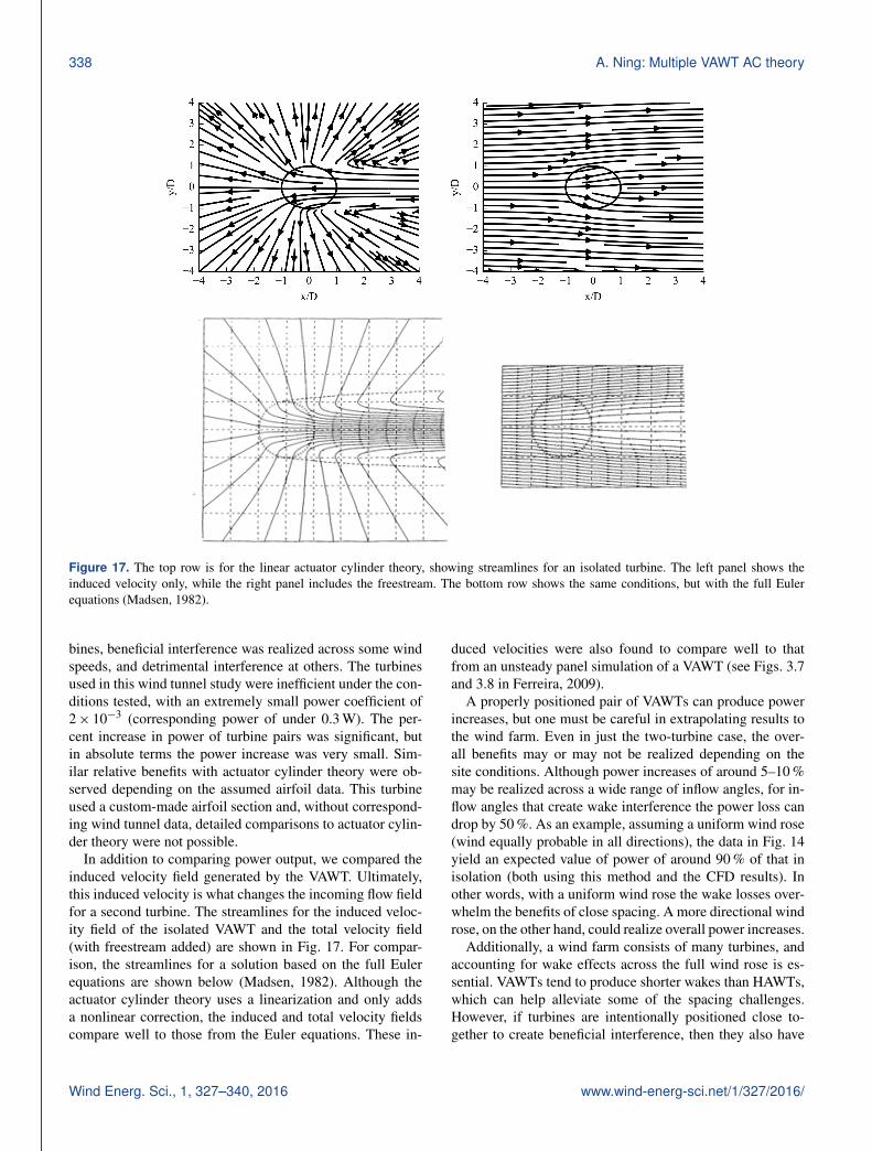
Figure 17. The top row is for the linear actuator cylinder theory, showing streamlines for an isolated turbine. The left panel shows theinduced velocity only, while the right panel includes the freestream. The bottom row shows the same conditions, but with the full Eulerequations (Madsen, 1982).

bines, beneficial interference was realized across some windspeeds, and detrimental interference at others. The turbinesused in this wind tunnel study were inefficient under the con-ditions tested, with an extremely small power coefficient of2× 10−3 (corresponding power of under 0.3 W). The per-cent increase in power of turbine pairs was significant, butin absolute terms the power increase was very small. Sim-ilar relative benefits with actuator cylinder theory were ob-served depending on the assumed airfoil data. This turbineused a custom-made airfoil section and, without correspond-ing wind tunnel data, detailed comparisons to actuator cylin-der theory were not possible.

In addition to comparing power output, we compared theinduced velocity field generated by the VAWT. Ultimately,this induced velocity is what changes the incoming flow fieldfor a second turbine. The streamlines for the induced veloc-ity field of the isolated VAWT and the total velocity field(with freestream added) are shown in Fig. 17. For compar-ison, the streamlines for a solution based on the full Eulerequations are shown below (Madsen, 1982). Although theactuator cylinder theory uses a linearization and only addsa nonlinear correction, the induced and total velocity fieldscompare well to those from the Euler equations. These in-

duced velocities were also found to compare well to thatfrom an unsteady panel simulation of a VAWT (see Figs. 3.7and 3.8 in Ferreira, 2009).

A properly positioned pair of VAWTs can produce powerincreases, but one must be careful in extrapolating results tothe wind farm. Even in just the two-turbine case, the over-all benefits may or may not be realized depending on thesite conditions. Although power increases of around 5–10 %may be realized across a wide range of inflow angles, for in-flow angles that create wake interference the power loss candrop by 50 %. As an example, assuming a uniform wind rose(wind equally probable in all directions), the data in Fig. 14yield an expected value of power of around 90 % of that inisolation (both using this method and the CFD results). Inother words, with a uniform wind rose the wake losses over-whelm the benefits of close spacing. A more directional windrose, on the other hand, could realize overall power increases.

Additionally, a wind farm consists of many turbines, andaccounting for wake effects across the full wind rose is es-sential. VAWTs tend to produce shorter wakes than HAWTs,which can help alleviate some of the spacing challenges.However, if turbines are intentionally positioned close to-gether to create beneficial interference, then they also have



the potential to create strong power losses through wake ef-fects.

Beneficial interference may be possible not just for pairsof turbines, but for carefully positioned arrays of turbines,as demonstrated in 2-D URANS simulations (Bremseth andDuraisamy, 2016). However, the benefits have only been ex-plored with one wind direction. Our past research in HAWTwind farm optimization suggests that when optimizing tur-bine positioning under uncertainty of wind direction, the op-timal configurations spread out and are not in aligned rowsin order to minimize wake interference (Fleming et al., 2016;Gebraad et al., 2016). Further investigation is needed to bet-ter understand how to optimize VAWT farms.

4 Conclusions

Actuator cylinder theory is a fast and often effective analysismethod to predict aerodynamic loads and power of verticalaxis wind turbines. In this paper we derive an extension to ac-tuator cylinder theory for multiple interacting turbines. Addi-tional extensions were provided that apply to both the single-turbine and multiple-turbine cases: thrust coefficients outsideof the momentum regions, and curved or swept blades.

Comparisons to published data for VAWT pairs showedreasonable agreement in predicting relative power changesand induced velocities using actuator cylinder theory. How-ever, more data are needed to better assess the conditions un-der which the multiple actuator cylinder theory is effective.Like blade element momentum methods, the accuracy andusefulness of actuator cylinder theory is highly dependent onproviding accurate airfoil coefficient data.

For closely spaced VAWTs, we observed cases with bene-ficial interference across a wide range of inflow angles, withpeak power increases exceeding 10 %. In other cases, detri-mental interference was observed. The conditions that affectthe interactions depend on many things, including the airfoilaerodynamic performance, the tip-speed ratios, and solidi-ties. Our focus here is to demonstrate the actuator cylindertheory and not to make a thorough investigation of closelyinteracting VAWTs, but more illumination on this topic isneeded.

Further improvements to actuator cylinder theory areneeded, as are more detailed validation studies. An improvedwake model is necessary because the wakes in actuator cylin-der theory are inviscid, do not decay, and do not spread. Ourrecent work has developed the first VAWT wake model de-rived from computational fluid dynamics simulations that isparametrized for turbines with different tip-speed ratios andsolidities (Tingey and Ning, 2016). Models like this couldbe combined with actuator cylinder theory to better predictturbine–wake interactions.

Because of the model’s sensitivity to the airfoil data, fur-ther data collection and improved methods of applying ro-tational corrections specific to VAWTs may be needed. Al-

though the method was only demonstrated in 2-D, as outlinedin the methods section, extensions to 3-D are straightforwardusing a strip-wise approach, but tip-loss corrections shouldbe added. Additionally, appropriate methods for accountingfor losses through struts and the tower will likely improveaerodynamic performance estimates.

5 Data availability

Source code for my implementation of this actuator cylindermethod has been made publicly available (Ning, 2016a), aswell as code and supplementary files used to generate thedata figures in this paper (Ning, 2016b).

Edited by: J. MeyersReviewed by: two anonymous referees

References

Ahmadi-Baloutaki, M., Carriveau, R., and Ting, D. S.-K.: Perfor-mance of a vertical axis wind turbine in grid generated turbu-lence, Sustainable Energy Technologies and Assessments, 11,178–185, doi:10.1016/j.seta.2014.12.007, 2015.

Araya, D. B., Craig, A. E., Kinzel, M., and Dabiri, J. O.: Low-ordermodeling of wind farm aerodynamics using leaky Rankine bod-ies, Journal of Renewable and Sustainable Energy, 6, 063118,doi:10.1063/1.4905127, 2014.

Bravo, R., Tullis, S., and Ziada, S.: Performance testing of a smallvertical-axis wind turbine, in: Proceedings of the 21st CanadianCongress of Applied Mechanics (CANCAM07), 3–7 June 2007,Toronto, Canada, 2007.

Bremseth, J. and Duraisamy, K.: Computational analysis of verticalaxis wind turbine arrays, Theor. Comp. Fluid Dyn., 30, 387–401,doi:10.1007/s00162-016-0384-y, 2016.

Buhl Jr., M. L.: A New Empirical Relationship between ThrustCoefficient and Induction Factor for the Turbulent WindmillState, National Renewable Energy Laboratory, Technical Report,NREL/TP-500-36834, 7 pp., 2005.

Burton, T., Jenkins, N., Sharpe, D., and Bossanyi, E.: Wind EnergyHandbook, 2nd Edn., Wiley, UK, 2011.

Claessens, M.: The Design and Testing of Airfoils for Applicationin Small Vertical Axis Wind Turbines, Master’s thesis, Delft Uni-versity of Technology, the Netherlands, 2006.

Dabiri, J. O.: Potential Order-of-Magnitude Enhancement of WindFarm Power Density Via Counter-Rotating Vertical-Axis WindTurbine Arrays, Journal of Renewable and Sustainable Energy,3, 043104, doi:10.1063/1.3608170, 2011.

Ferreira, C. S.: The Near Wake of the Vawt, PhD thesis, Delft Uni-versity of Technology, the Netherlands, 2009.

Ferreira, C. S., Madsen, H. A., Barone, M., Roscher, B., Deglaire,P., and Arduin, I.: Comparison of Aerodynamic Models for Ver-tical Axis Wind Turbines, J. Phys. Conf. Ser., 524, 012125,doi:10.1088/1742-6596/524/1/012125, 2014.

Fleming, P., Ning, A., Gebraad, P., and Dykes, K.: Wind Plant Sys-tem Engineering through Optimization of Layout and Yaw Con-trol, Wind Energy, 19, 329–344, doi:10.1002/we.1836, 2016.

Gebraad, P., Thomas, J. J., Ning, A., Fleming, P., and Dykes, K.:Maximization of the Annual Energy Production of Wind Power


http://dx.doi.org/10.1016/j.seta.2014.12.007

http://dx.doi.org/10.1063/1.4905127

http://dx.doi.org/10.1007/s00162-016-0384-y

http://dx.doi.org/10.1063/1.3608170

http://dx.doi.org/10.1088/1742-6596/524/1/012125

http://dx.doi.org/10.1002/we.1836


Plants by Optimization of Layout and Yaw-Based Wake Control,Wind Energy, doi:10.1002/we.1993, online first, 2016.

Hansen, M. O. L.: Aerodynamics of Wind Turbines, 2nd Edn.,Earthscan, London, UK, 2008.

Huskey, A., Bowen, A., and Jager, D.: Wind Turbine Generator Sys-tem Power Performance Test Report for the Mariah Windspire1-kW Wind Turbine, National Renewable Energy Laboratory,Technical Report, NREL/TP-500-46192, doi:10.2172/969714,2009.

Korobenko, A., Hsu, M.-C., Akkerman, I., and Bazilevs, Y.: Aero-dynamic Simulation of Vertical-Axis Wind Turbines, J. Appl.Mech., 81, 021011, doi:10.1115/1.4024415, 2013.

Madsen, H.: The Actuator Cylinder – a Flow Model for Verti-cal Axis Wind Turbines, PhD thesis, Aalborg University Centre,1982.

Madsen, H., Larsen, T., Vita, L., and Paulsen, U.: Implementa-tion of the Actuator Cylinder Flow Model in the HAWC2 Codefor Aeroelastic Simulations on Vertical Axis Wind Turbines, in:51st AIAA Aerospace Sciences Meeting, 7–10 January 2013,Grapevine, Texas, AIAA 2013-0913, doi:10.2514/6.2013-913,2013.

Manwell, J. F., Mcgowan, J. G., and Rogers, A. L.: Wind EnergyExplained, 2nd Edn., Wiley, UK, 2009.

Ning, A.: A Simple Solution Method for the Blade Element Mo-mentum Equations with Guaranteed Convergence, Wind Energy,17, 1327–1345, doi:10.1002/we.1636, 2014.

Ning, A.: VAWT AC, Zenodo, doi:10.5281/zenodo.165183, 2016a.Ning, A.: VAWT AC Supplementary Files, figshare,

doi:10.6084/m9.figshare.3382504.v3, 2016b.Paraschivoiu, I.: Double Multiple Streamtube Model for Darrieus

Wind Turbines, in: 2nd DOE/NASA Wind Turbine DynamicsWorkshop, 24–26 February 1981, Cleveland, OH, 1981.

Paraschivoiu, I.: Double-multiple streamtube model for study-ing vertical-axis wind turbines, J. Propul. Power, 4, 370–377,doi:10.2514/3.23076, 1988.

Paraschivoiu, I. and Delclaux, F.: Double Multiple StreamtubeModel with Recent Improvements (for Predicting AerodynamicLoads and Performance of Darrieus Vertical Axis Wind Tur-bines), J. Energy, 7, 250–255, doi:10.2514/3.48077, 1983.

Sheldahl, R. E. and Klimas, P. C.: Aerodynamic characteristics ofseven symmetrical airfoil sections through 180-degree angle ofattack for use in aerodynamic analysis of vertical axis wind tur-bines, Sandia National Labs., Albuquerque, NM, USA, TechnicalReport, SAND80-2114, doi:10.2172/6548367, 1981.

Strickland, J.: A performance prediction model for the Darrieus tur-bine, in: International Symposium on Wind Energy Systems, 1,3 pp., 1975.

Templin, R.: Aerodynamic performance theory for the NRCvertical-axis wind turbine, LTR-LA-160, National AeronauticalEstablishment, Ottawa, Ontario, Canada, 1974.

Tingey, E. and Ning, A.: Parameterized Vertical-Axis Wind Tur-bine Wake Model Using CFD Vorticity Data, in: ASMEWind Energy Symposium, 4–8 January 2016, San Diego, CA,doi:10.2514/6.2016-1730, 2016.

Wilson, R. and Lissaman, P.: Applied Aerodynamics of Wind PowerMachines, Oregon State University, Tech. rep., 109 pp., 1974.

Zanforlin, S. and Nishino, T.: Fluid dynamic mechanismsof enhanced power generation by closely spaced verti-cal axis wind turbines, Renew. Energ., 99, 1213–1226,doi:10.1016/j.renene.2016.08.015, 2016.



http://dx.doi.org/10.2172/969714

http://dx.doi.org/10.1115/1.4024415

http://dx.doi.org/10.2514/6.2013-913


http://dx.doi.org/10.5281/zenodo.165183

http://dx.doi.org/10.6084/m9.figshare.3382504.v3

http://dx.doi.org/10.2514/3.23076

http://dx.doi.org/10.2514/3.48077

http://dx.doi.org/10.2172/6548367

http://dx.doi.org/10.2514/6.2016-1730

http://dx.doi.org/10.1016/j.renene.2016.08.015

actuator cylinder theory for multiple vertical axis … cylinder theory for multiple vertical axis...

Documents