ad/a-002 261 geometric modeling for computer vision …
TRANSCRIPT
■ ' ' '
AD/A-002 261
GEOMETRIC MODELING FOR COMPUTER VISION
Bruce Guenther Baumgart
Stanford University
^
Prepared for:
Office of Naval Research Advanced Research Projects Agency
October 1974
DISTRIBUTED BY:
Knn© National Technical Information Service U. S. DEPARTMENT OF COMMERCE
..—•
^» ^n

*m^
UNCLASSIFIED SECURITY CLAaSIFICATION OF THIS PAGE (When Data F.ntrred)
REPORT DOCUMENTATION P£GE 1. REPORT NUMBER
siM-cs-74-WJ; 2. GOVT ACCESSION NO
4. TITLE fand Si/bl/((e;
GEOMETRIC MODELING FOR COMPUTER VISION
READ INSTRUCTIONS BEFORE COMPLETING FORM
3. RECIPIENT'S CATALOG NUMBER
5. TYPE OF REPORT 4 PERIOD COVERED
technical, Oct., 197»+
7. AUTHORCO
Bruce Guenther Bauragart
6. PERFORMING ORG. REPORT NUMBER
STAN-CS-T^ÖS 8. CONTRACT OR GRANT NUMBERfsO
DAHC l^-73-C-Oi+35
9. PERFORMING ORGANIZATION NAME AND ADDRESS
Stanford University Computer Science Department Stanford, California 9^30^
II. CONTROLLING OFFICE NAME AND ADDRESS
ARPA/lPT, Attn: Stephen D. Crocker, 1400 Wilson Blvd., Arlington, Va. ccc09
10. PROGRAM ELEMENT, PROJECT, TASK AREA & WORK UNIT NUMBERS
12, REPORT DATE
October, 197^
14. MONITORING AGENCY NAME S ADDRESSfi/ ditleiint Irzm CorKrolling Olllce)
ONR Representative: Philip Surra Durand Aeronautics Bldg., Em. 165 Stanford University Stanford, California
13. NUMBER OF PAGES
IS. SECURITY CLASS, (of this report)
UNCLASSIFIED 15a DECLASSIFICATION/DOWNGRAD1NG
SCHEDULE
16. DISTRIBUTION STATEMENT (ol this Report)
Roleasable without limitations on dissemination.
17. DISTRIBUTION STATEMENT (ol the abS(racl entered in Block 20. II dlllerent Iron, Report)
18. SUPPLEMENTARY NOTES
Reproduced by
NATIONAL TECHNICAL INFORMATION SERVICE
US Dopartmont o( Commorco Springfield, VA. 22151
19. KEY WORDS fCon((nue on reverse aide il necessary and identlly by block number)
20. ABSTRACT (Continue on reverse side If necessary end Idenlily by tiock number)
The main contribution of this thesis is the development of a three dimensional geometric modeling system foi application to computer vision. In computer vision geometric models provide a goal for descriptive image analysis, an origin for verification image synthesis, and a context for spatial problem solving. Some of the design ideas presented have been implemented in two programs named GE0MED and CRE; the programs are demonstrated in situations involving camera motion relative to a static world.
DD FORM 1 JAN 73 1473 EDITION OF 1 NOV 65 IS OBSOLETE UNCLASSIFIED
» SECURITY CLASSIFICATION OF THIS PAGE fWien Da(a E.Kered;
^rita

i
I I I [
I I I 1
1
I I I I
SECTION 0.
TABLE OF CONTENTS.
INTRODUCTION. PAGE 1.
SECTION 1. GEOMETRIC MODELING THEORY. PAGE 6.
1.0 Introduction to Geometric Modeling 6 1.1 Kinds of Geometric Models 7 1.2 Polyhedron Definitions and Properli« 12 1.3 Camera, Light and Image Modeling 13 1A Related Modeling Work 14
SECTION 2. THE WINGED EDGE POLYHEDRON REPRESENTATION. PAGE 15.
2.0 Introduction to the Winged Edge 15 2.1 Winged Edge Link Fields 17 2.2 Sequential Accessing 19 2.3 Perimeter Accessing 19 2.4 Basic Polyhedron Synthesis 21 2.5 Edge and Face Splitting 23 2.6 Coordinate Free Polyhedron Representation 26
SECTION 3. A GEOMETRIC MODELING SYSTEM. PAGE 27.
3.0 Introduction to GEOMED 27 3.1 Euler Primitives 30 3.2 Routines using Euler Primitives 34 3.3 Euclidean Routines 37 3.4 Image Synthesis: Perspective Projection and Clipping 43 3.5 Image Analysis: Interface to CRE 44
SECTION 4. HIDDEN LINE ELIMINATION FOR COMPUTER VISION. PAGE 46.
4.0 Introduction to Hidden Line Elimination 46 4.1 Initialization and Culling 48 4.2 Hide Marking a Coherent Object 51 4.3 Edge-Edge and Face-Vertex Comparing 52 4.4 Recursive Windowing 55 4.5 Photometric Modeling and Video Generation 58 4.6 Performance of OCCULT and Related Work 59
SECTION 5. A POLYHEDRON INTERSECTION ALGORITHM. PAGE 60.
5.0 Introduction to Polyhedron Intersection 60 5.1 Intersection Geometry 62 5.2 Intersection Topology 63 5.3 Special Cases of Intersection 65 5.4 Face Convexity Coercion 66 5.5 Body Cutting 66 5.6 Performance and Related Work 67
/
•i
^fei m*

^»
TABLE OF CONTENTS.
SECTION 6. COMPUTER VISION THEORY. PAGE 68.
6.0 Introduclion to Computer Vision Theory 68 6.1 A Geometric Feedback Vision System y 6.2 Vision Tasks . 6.3 Vision System Design Arguments '* 6.4 Mobile Robot Vision 77
6.5 Summary and Related Vision Work '9
SECTION 7. VIDEO IMAGE CONTOURING. PAGE 82.
7.0 Introduction to Image Analysis ** 7.1 CRE - An Image Processing System »* 7.2 Thresholding !! 7.3 Contouring 7.4 Polygon Nesting " 7.5 Contour Segmentation '* 7.6 Related and Future Image Analysis "
SECTION 8. IMAGE COMPARING. PAGE 95.
8.0 Introduction to Image Comparing 95 8.1 A Polygon Matching Method ^ 8.2 Geometric Normalization of Polygons 9° 8.3 Compare by Recursive Windowing '00 8.4 Related Work and Work Yet To Be Done »0°
SECTION 9. CAMERA AND FEATURE LOCUS SOLVING. PAGE 101.
9.0 Introduction to Locus Solving JO* 9.1 Parallax and the Camera Model 0* 9.2 Camera Locus Solving: One View of Three Points 104 9.3 Object Lotus Solving: Silhouette Cone Intersection 109 9.4 Sun Locus Solving: A Simple Solar Ephemeris j j|| 9.5 Related and Future Locus Solving Work ' 15
SECTION 10. RESULTS AND CONCLUSIONS. PAGE 116.
10.1 Results: Accomplishments and Original Contributions | |j| 10.2 Critique: Errors and Ommissions J J° 10.3 Suggestions for Future Work j * * 10.4 Conclusion
SECTION 1L ADDENDA. PAGE 124.
11.1 References } ~* 11.2 GEOMED Node Formats ,'»1
1
/

^^—I-
I I I
SECTION 0
SECTION I.
SECTION 2
SECTION 3.
SECTION fl
SECTION 5
SECTION 6
.. j
* SECTION 7
SECTION 8
SECTION 9
SECTION 10
1
LIST OF BOXES.
INTRODUCTION
GEOMETRIC MODELING THEORV I | Ten Kmdi of Geometric Model« 7
1 2 De»ir»blo Properlic« for a Geometric Model 11
1.3 Properties of Polyhedre 12
THE WINGED EDGE POLYHEDRON REPRESENTATION 2.1 Winced EdRe Structure! and Linkt 17 2.2 Lowe«t Level Winded Edge Routine« 21
A GEOMETRIC MODELING SYSTEM 3 | The Euler Primitive« 31 3 2 Routine« U«in(; the Euler Primitive« 34
33 Euclidean Transformations 38
3fl Tram Routmo« 39 3 5 Metric Poutmp« 42
3 6 Simple Space Routines 42
HIDDEN LINE ELIMINATION FOR COMPUTER VISION. q | Five Hidden Line Elimination Technique» 48 4 2 Status Bits for Occult Marking 49
4 3 Normalized Face and Edge Coefficient» BO
4 4 Edge-Edge Compare Step« 53 4 5 Recursive Windowing routine»...
A POLYHEDRON INTERSECTION ALGORITHM
56
COMPUTER VISION THEORY
61 62 63 64 65 66 67
68
Vision System Hierarchy 69 Three Basic Modes of Vision 69 Basic Feedback Vision System Deeign 70
Processors of a 3-0 Vision Sy»t»m 71
Six Eiamples of Computer Vision T»»k» 72 Alternative» to 3-D Geometric Modeling 75
Cart Vision Mandala 77 A Possible Cart Task Solution 78
VIDEO IMAGE CONTOURING 7 I CRE Design Choices 84
7 2 CRE Data Transformations 86
IMAGE COMPARING
CAMERA AND FEATURE LOCUS SOLVING
RESULTS AND CONCLUSIONS 10.1 Accomplishment» and Original Contribution» 116
10.2 Suggeelion» for Future Work 1 19
I III -
^^w
LIST OF FIGURES.
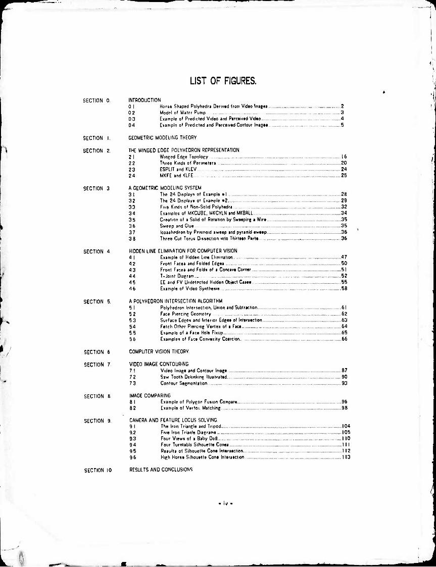
SECTION 0. INTRODUCTION 0 I Hone Shaped Polyhedn Derived from Video Imigee 2 0 2 Modol of Water Pump 3 03 Example of Predicted Video and Perceived Video 4 0 4 Examplo of Predicted and Perceived Contour Imagee 5
SECTION I. GEOMETRIC MODELING THEORY
SECTION 2. THE WINGED EDGE POLYHEDRON REPRESENTATION 2 I WinRpd Edfje Topology 16 22 Three Kinds of Perimeter» 20 2 3 ESPLIT and KLEV 24 24 MKFE and KLFE 25
SECTION 3 A GEOMETRIC MODELING SYSTEM 3,1 The 24 Display« of Example «1 28 3 2 The 24 Displays of Example »2 29 33 Five Kinds of Non-Sohd Polyhedr» 32 3 4 Examples of MKCU8E, MKCYLN and MKBALL 34 3 5 Creation of a Solid of Rotation by Sweeping a Wire 35 3 6 Sweep and Glue 35 3 7 Icosahedron by Prisrnoid sweep and pyramid sweep 36 3 8 Three Cut Torus Dissection into Thirteen Part« 36
I
SECTION 4 HIDDEN LINE ELIMINATION FOR COMPUTER VISION 4 I Example of Hidden Line Elimination 47 4 2 Front Face» and Folded Edge» 50 43 Front Faces and Folds of I Concave Corner 51 4 4 T-Joint Diagram 52 4 5 EE and FV Undetected Hidden Object Case» 55 4 6 Example of Video Synthesis 58
SECTION 5 A POLYHEDRON INTERSECTION ALGORITHM 5 I Polyhedron Intersection, Union and Subtraction 61 5 2 Face Piercing Geometry 62 53 Surface Edges and Interior Edge» of Intereection 63 54 Fetch Other Piercing Vertex of a Face 64 5 5 Example of a Face Hole Fixup 65 5 6 Examples of Fjc» Convexity Coercion 66
SECTION 6 COMPUTER VISION THEORY
SECTION 7 VIDEO IMAGE CONTOURING 7 1 Video Image and Contour Image 87 7 2 Saw Tooth Dekmking Illustrated 90 7 3 Contour Segmentation 93
SECTION 8
SECTION 9
SECTION 10
IMAGE COMPARING 8 1 Example of Polygon Fusion Compare 96 8 2 Example of Vertoi. Matching 98
CAMERA AND FEATURE LOCUS SOLVING 9 I The Iron Triangle and Tripod 104 9.2 Five Iron Trianle Diagram» 105 9.3 Four View» of a Baby Doll 1 10 94 Four Turntable Silhouette Cone» 111 95 Results of Silhouette Con« Inteneclion 112 9 6 High Horse Silhouette Con« Intersection 1 13
RESULTS AND CONCLUSIONS
/

^^*-
ACKNOWLEDGEMENTS.
The following people personally contributed to this work:
Thesis Adviser: John McCarthy Readers: Donald E. Knuth, Alan C. Kay, Ken Colby.
Jerry Aein, leona Baumgart, Tom Binford, Jack Buchanan, Whitfield Diffie, Les Earnest, Jerome Feldman, Tom Gafford, Steve Gibson, Ralph Gorin, Carl Hewitt, Jack Holloway, Tovar Mock,
Andy Moorer, Hans Moravec, Richard Orban, Ted Panofsky, Lou Paul, Phil Petit, Dave Poole, Lynn Quam, Jeff Raskin, Ron Rivest, Rod Schmidt, Clem Smith, Irwin Sobel, Robert Sproull,
Dan Swinehart, Russell Taylor, Marty Tenenbaum, Larry Tesler, Arthur Thomas, Fred Wright.
TYPOGRAPHY
The oreinal copy of this document was produced on a Xerox Graphics Printer with a resolution of two hundred points per inch. The principal font is News Gothic Boldface, 25 units h.gh, which orieinated at Carnegie Mellon University. The page layout, text justificat.on, boxes, halftones and line drawings were done using the author's document-formating program, X1P. The source files were
prepared using the text editor, E, created by Dan Swinehart and Fred Wright.
,
/
-"- ^- » . - ~w . ~ ^h_—t—^^^^^

w^^
INTRODUCTION.
SECTION 0.
INTRODUCTION.
"Tor ihr iJurposo of prrsrnlinß my arpumrnl I musl first explain the basic premise of sorcery as
ilon Juan presented it to me. He said thai for a sorcerer, the world of everyday life is not real, or out
there, as we believe it is. For a sorcerer, reality or the world we all know, is only a description. For the sake of validating this prntnisn don Juan concentrated the best of his efforts into leading mc to a
genuine conviction that what I held in mind as the world at hand was merely a description of the world;
a description that had been pounded into mc from the moment I was born.
- Carlos Castaneda. journey to Ixtlan.
I I I
This thesis is about computer techniques for handling 3-D geometric descriptions of the world;
the world that can be visually perceived with a television camera. The overall design idea may be
characterized as an inverse computer graphics approach to computer vision. In computer graphics, the
world is represented in sufficient detail so that the image forming process can be numerically simulated
to generate synthetic television images; in the inverse, perceived television pictures (from a real TV
camera) are analysed to compute detailed geometric models. For example, the polyhedra in Figure 0.1
on page two were computed from views of a plastic horse on a turntable. It is hoped, that visually
acquired 3-D geometric models can be of use to other robotic processes such as manipulation,
navigation or recognition.
- 1 -
m** «M

mm*
INTRODUCTION.
FIGURE 0.1 - HORSE SHAPED POLYHEDRA DERIVED FROM VIDEO IMAGES.
I I I I I I
I
Arita
^•i
INTRODUCTION.
I
.
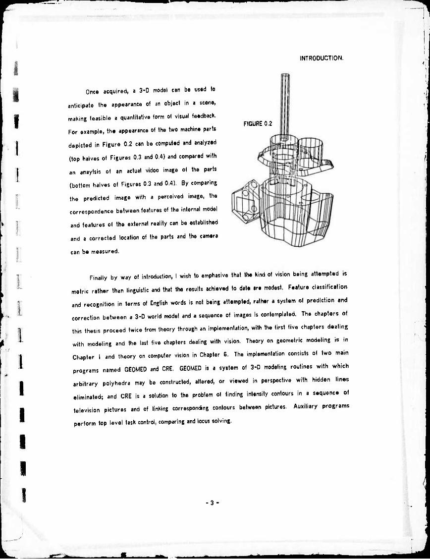
Once acquired, a 3-D model can be used to
anticipate the appearance of an object in a scene,
making feasible a quantitative form of visual feedback.
For example, the appearance of the two machine parts
depicted in Figure 0.2 can be computed and analyzed
(top halves of Figures 0.3 and 0.4) and compared with
an anaylsis of an actual vidoo image of the parts
(bottom halves of Figures 0,3 and 0.4). By comparing
the predicted image with a perceived image, the
correspondence between features of the internal model
and features of the external reality can be established
and a corrected location of the parts and the camera
can be measured.
FIGURE 0.2
I I I I I
Finally by way of introduction, I wish to emphasive that the kind of vision being attempted is
metric rather than linguistic and that the results achieved to date are modest, Feature classification
and recognition in terms of English words is not being attempted, rather a system of prediction and
correction between a 3-D world model and a sequence of images is contemplated. The chapters of
this thesis proceed twice from theory through an implementation, with the first five chapters dealing
with modeling and the last five chapters dealing with vision. Theory on geometric modeling is in
Chapter 1 and theory on computer vision in Chapter 6. The implementation consists of two main
programs named GE0MED and CRE. GEOMED is a system of 3-D modeling routines with which
arbitrary polyhedra may be constructed, altered, or viewed in perspective with hidden lines
eliminated; and CRE is a solution to the problem of finding intensity contours in a sequence of
television pictures and of linking corresponding contours between pictures. Auxiliary programs
perform top level task control, comparing and locus solving.
3-

mm^
INTRODUCTION.
flililliliiifillilf11 |{||ll||P|ll|!l|l||i||l||lil||l!l||lll!| !|l|l|ll|PiP|illPIP|||PPPIilPi!iPPililllliM^^
'" (I iiiiii1'1''''li PI
11
P 11 Uti'ii
J , .11 «i .y^' ' '
i 'I'M l!1i<'|ill I'll
' ■: :/• ■ ■'■;:i!ffiiiJllt;! i!
0 Ä,A"Ä
■ ■:■ J!l ii ' . I I ÜiÜI Ulli I
iilliliiiilto,,.'! Ililll
! ,
illlli'tll,,. 1 iii I Illlllilii
11 ■'::l„ ill I !|
i;iiii|iih';!i1i;y-i;vii!n'W tin1 ;,,,.,,.,,,.:
V,;III,:T:;N ■ !
!
'■'^t
li ill III lllf
ill |||ll!lli:;
lllllll!
ill ||l!i!
iil IS!
liiili l |j||||i!.;i|;i • ■, ■ ; •' -' i; il'in
|| I im I ; :l J 11 H
ii i,,'il"iil HI1 n i i'. - ii '
■ ' '' ■ ;
[ill i II
;i|f iPlil!
i'i
.:;- i ililll ■;..,,:.; I,il lui ||| |||||||j mil
ip I I iiij iiiibi,.
FIGURE 0.3 - PREDICTED VIDEO t AND PERCEIVED VIDEO i
MlllliiillMilMli
I i
I illilltl
Mm iliiPPIIP'll
i I'Sn: I11!1
lllllll illpljl
llilllllii
II
ililii|ii|{l ii|i||||; IM i'liifiiw ■':-"■' if ;i] PPIlillllllllililllllillilPllllliJlliP^
111 ili'li" HI
" i ill II
IP!
i.,,:
Ti ^"TI'IHI'TI, llin'*'.'' jUPiiii i:|
: 1
I'll'; ,„
■r,i, '
I III /i,m
#
liilllllli,
liinflll-luil:,!,!, ullli ''IM-j'Ji1'!! | llllJi
,■:.:,„
111'! .
1, :l'llil
-'^■lü' mi
mm I- ii
lllllll1«1" jigl
■•;, , jl.i
i
l'1':iii:!l;i|ll I ili it^iiih III in
i ■ I 'li1 llnlll
ill lilliii 'W ll||iill||l
:- -■:|:!lliji!
;,ill;l||, ■l'I'l'. ,.'I':11I;I1' ■I'llM llii''«Il
.gmp WBii " iil
lillllll!'! 'Uli »«I Hi" 'I'liii''
iiii' .iLli'l
-!i!N! r , J;,| i.il'iil.i1, J|:,J,,1!
I pil |l lll!l|l
'illlii lllllll
r«.! : 'm;,i;: IIIHHII lilin • ■ ■ '
■l ..:•■ .IIIJ
,,,!•,
:."„ "''III I :,,'■■ illl'
ill f liiili
Hu1"1 in '1 il!il|
;...,::....,:,i: ,, lii^iillllillliyiiliililllli 11
i iii;11! lib ■■i'lllil.i!
P IPII'I I ' 11 IIk;iihi ii'1 ■ '' ■ lllllililliililliillll! ii'ivi'i.
'lil. Hii
mwmMmmm iiiaii:ii"«S R il«ill "M^li' , b' :,'■,,:•
lllllll
I: III IIII1 ill
M i l^iplil It
Ill 1 iillliiililililiiillllillll
^■h ^*m

INTRODUCTION.
I I I I I
1 I I
FIGURE 0.4 - PREDICTED IMAGE T AND PERCEIVED IMAGE i.
I
^k^B^M

I 1.0 Introduction to Geometric Modeling. GEOMETRIC MODELING THEORY.
SECTION 1.
GEOMETRIC MODELING THEORY.
1.0 Introduction to Geometric Modeling. 1.1 Kinds ot Geometric Models. 1.2 Polyhedron Definitions and Properties. 1.3 Camera, Light and Image Modeling.
1.4 Related Modeling Work.
1,0 Introduction to Geometric Modeling.
In the specific context of computer vision and graphics, geometric modeling refers to the
construction of computer representations of physical objects, cameras, images and light for the sake of
simulating their behavior. In Artificial Intelligence, a geometric model is a kind of world model;
ignoring subtleties, geometric world modeling is distinguished from semantic and logical world modeling
in that it is quantitative and numerical rather than qualitative and symbolic. The notion of a world model
requires an external world environment to be modeled, an internal computer environment to hold the
model, and a task-performing entity to use the model, In Geometry, modeling is a synthetic problem,
like a construction with ruler and straight edge; modeling problems require an algorithmic solution
rather than a proof. The word grometric. is an appropriate adjective to this kind of modeling in that it
is a combination of the Greek words yno (world) and jurp»« (measuring) which is exactly the activity to
be automated.
.
^di mam

1.1 Kinds of Geometric Models.
1.1 Kinds of Geometric Models.
GEOMETRIC MODELING THEORY.
Th« main problem of geometric modeling is to invent methods for represtmting arbitrary
physical objects in i computer. For the present discussion, the class of physical objects is restricUd to
objects that are solid, rigid, opaque, and macroscopic with a mathematically well behaved surface. Such
objects include: the earth, chairs, roads, and plastic toy horses; other objects, for which models will not
be attempted, include glass, fog, hair, Jello, liquids and cloth. Physical objects can move about in space
with the restriction that two objects can not occupy the same space at the same time. The scope of the
modeling problem can be appreciated by examining the models listed in Box 1.1,
BOX 1.1 TEN KINDS OF GEOMETRIC MODELS.
Space Oriented: 1. 3"D Space Array. 2. Recursive Cells. 3. 3-D Density Function. 4. 2-D Surface Functions. 5. Parametric Surface Functions.
Object Oriented: 6. Manifolds. 7, Polyhedra, 3. Volume Elements. 9. Cross Sections. 10. Skeletons.
For a naive start, first consider a 3-D array in which each element indicates the presence or
absence of solid matter in a cube of space. Such a 3-D space array has the very desirable properties
of ipatial addrcning and »patial uniquenm in their most direct and natural form. Spatial addressing
refers to finding out what the model contains within a distance R of a locus X,Y,Z; spatial uniqueness
refers to the property that physical solids can not occupy the same space simultaneously. A first
drawback of the space array idea is illustrated by the apparently legal FORTRAN statement:
DIMENSION SPACE(100000,100000,100000)
The problem with such a dimension statement is that no present day computer memory is large enough
to contain a ID15 element array. Smaller space arrays can be useful but necessarily can not model
large volumes with high resolution. A further drawback of space arrays is that objects and surfaces
are not readily accessible as entities; that is a space array lacks the property of ohjeet coherence. In
computer graphics, the term coherml denotes both the quality of holding together as parts of the same
mass and the quality of not changing too drastically from one point to the next. The meaning of
coherent approachs the mathematical notion of topologically connected and locally continuous. The word
is used to refer to the frame coherence of a film as well as to the object coherence of a model.
1 i I I I I I I I
I
i i
*
tf^ta rtM

I I I I i I I I !
1
1.1 Kinds of Ger-ielric Models. GEOMETRIC MODELING THEORY.
The space array idea can be salvaged by grouping blocks of elements with the same value
together; the addressing process becomes more complicated but the overall memory required is
reduced and the two desired properties can be maintained. One way of doing this (which has been
discovered in several applications) is rrrunit* rrlh-, the whole space is considered to be a cell; if the
space is not homogeneous then the first cell is divided into two (or four or eight) sub cells and the
criterion is applied again. This technique allows the spatial sorting of objects when the object models
can be subdivided at each recursion without losing their properties as objects.
Another salvageable naive modeling idea is that arbitrary objects can be expressed as algebraic
functions. In physics, physical objects are frequently referred to as three dimensional density functions
W«p(X,Y,Z). Unfortunately such density functions can no» be writtrn out for objects such as a typing
chair or a plastic horse without resorting to a programming language or an extensive table (which is
equivalent to the space array model). Objects that are essentially 2-D can be approximated by a
surface function 2 = F(X,Y). For example landscape may be represented by geodetic maps in such a
2-D fashion.
By definition, a function is single valued; consequently the description of even modestly
complicated objects cannot be expressed by giving one coordinate, e.g. 2, as a function of the other
two, e.g. X and Y. It is necessary either to adopt parametric functions or to subdivide the object into
portions that can be described by simple functions of Cartesian variables. The former course involves
establishing a system of surface coordinates (U,V), latitudes and longitudes, on the object in which
functions for the X,Y,2 locus of the object's surface are expressed. The advantage of parametric
functions is that extended arbitrary curve surfaces can be expressed; some of the disadvantages are
that parametric curves may be self intersecting, they are not easy to modified locally, and the functions
become impractical before the shapes of mundane artifacts can be achieved. Consequently parametric
representations are combined with object subdivision, which is called ngmcntmion. The process of
usefully segmenting an object without destroying its coherence is a major problem requiring the
combination of spatial, functional and objective representations.
8-

1.1 Kinds of Geometrie Models. GEOMETRIC MODELING THEORY.
In passing from space oriented models to object oriented models, I wish to not« that
sophisticated representation of time is beyond the scope of this worK. Although an advanced problem
solving robot will need to run world simulations along multiple time paths, the discussion will
concentrate on representing the geometry of the world at a single moment in time.
After existence in space and time, another general property of physical objects is that they can
be enclosed by an unbroken two dimensional surface with an unambiguous inside and outside; which
touchs upon the mathematical topic (celebrated in song by Tom Lehrer) of the algebraic topology of
locally Euclidean transitions of infinitely differentiable oriented Riemann manifolds. A manifold is the
mathematical abstraction of a surface; a Riemann manifold has a metric function; an oriontrd manifold
has • unambiguous inside and an outside; the phrase infinitdy differcntiahh can be taken to mean
that the surface is smooth; and the phrase locally Euclidean transition* refers to the process of
segmenting the object into portions that can be approximated by relatively simple functions. In
particular, the 2-0 Riemann submanifoid embedded in 3-D Euclidean space is the mathematical object
that comes closest to representing the shape and extent of the surface of a physical object; such
manifolds are conveniently approached through the topology of surfaces which in turn is
computationally approached by means of polyhedra.
One way to describe the topology of a 2-D Riemann submanifoid embedded in a 3-D Euclidean
space is in terms of three kinds of simplex: the O-Simplex (or vertex), the 1-Simplex (or edge), and
the 2-Simplex (or triangle). In topological analysis 2-D Riemann submanifolds may be divided into
faces, edges and vertices such that Euler's equation F-E»V«2*2»H is satisfied (where F is the number
of faces, E is the number of edges, V is the number of vertices and H is the genus or number of
handles of the manifold); and such that the surface of the manifold can be approximated by local
functions over each face which are Euclidean and which fit together smoothly at all the edges. By
introducing a sufficient (but finite) number of triangles the manifold can be approximated to within any
epsilon by constant functions, yielding the geometric object called the polyhedron.
One advantage of a polyhedral model is its connected surface topology of faces, edges and
vertices. Such a surface can be subdivided without losing its coherence or the coherence of the object.
I
I
rfm
1.1 Kinds of Geometrie Modeis. GEOMETRIC MODELING THEORY
The disadvantages of polyhedra include the lack of spatial uniqueness and spatial addressing wtvch
necessitates computation to be done to detect and prevent spatial conflict and to find the portions of an
entity occupying a given volume. Another feature of polyhedra (which can be an advantage or
disadvantage) is that all the (Gnuman) curvature happens suddenly at the vertices; however by
associating higher order approximation functions with each face the model of a continuous 2-0 manifold
can be made which is a more conventional curved object representation. Nevertheless, polyhedra are
intrinsically a general curved object representation.
I
I
I I I I 1
Returning to the survey, arbitrary objects can also be described by listing a set of cross
sections taken at a sufficient number of cutting planes; this is how the shape of a ship's hull or an
airplane's wing is specified. Cross sections have the interesting feature of good space modeling on one
axis. Forsaking arbitrary shaped objects, large classes of things can be described in terms of a small
set of basic volume elements. For example, Roberts (63)* and others have built models of familiar
objects using only rectangular and triangular right prisms. Arbitrary solid polyhedra can be
constructed out of tetrahedra (the 3-simplex); however no significant genera! modeling system exists
using this potentially interesting approach.
Skeletal models are based on abstracting an object into a stick figure and by associating a
diameter or set of cross sections with the sticks. In particular, spine cross section models have been
pursued at Stanford by Agin (72) and Nevatia (74). Spine cross section models have the advantage of
being able to express many objects in a concise form suitable for recognition, but they cannot be used
directly for arbitrary shapes.
Finally, it is often useful to represent physical objects by weak geometric models such as by
sets of spheres or by sets of unconnected surface points. It is interesting to note that ihe rrnlity that
the robot in Winograd's thesis (Winograd 71) could talk about, was a blocks world based on a geometric
model consisting only of points, sire of block, and a two page LISP subroutine named FINDSPACE.
* Parenthesized names and numerals are references listed in Section 11.1
10
m^mt^mmmmm^mm

1.1 Kinds of Geometrie Models. GEOMETRIC MODELING THEORY,
Beyond the particular kinds of geometric models, four general purpose modeling techniques
deserve special mention and isolation: prototype instance structure, parts tree structure, resolution
limited structure, and procedure generated structure. Superficially, the prototype instance structure is
a memory efficiency technique based on storing generalizations (prototypes) which can be bound to
specific cases (instances) as the occasion demands. Parts tree structure is a memory management
technique of organizing the whole universe of discourse as a tree data structure, where objects are
composed of subobjects. Resolution limited structure is a memory accessing technique, where
depending on a specified scale of interest different models are retrieved or even generated. Finally,
procedure generated structure concerns the trade-off between storing and recomputing a model;
namely recomputing the details of a model as they are needed is a good idea for extending
computational resources.
l I I
The danger to be avoided is to mistake the general modeling techniques for the geometric model
itself. Given a modeling regime it can be improved by prototyping, parts-treeing, resolution-limiting
and procedural-generating; without a good basic geometric model the general techniques amplify the
background noise.
BOX 1.2 DESIRABLE PROPERTIES FOR A GEOMETRIC MODEL.
^
1. Spatial addressing.
2. Spatial uniqueness.
3. Object coherence.
4. Surface coherence.
5. Shape generality.
6. Large extent with high resolution.
7. Easy modifiablity.
8. Suitability for physical simulation.
9. Efficiency of memory and computation use,
10. Suitability for automatic model acquisition.
To the best of my knowledge, this survey is complete. As of this year, 1974, there are no
other significantly different kinds of simple geometric models. The desirable properties that have
turned up in this survey are listed in Box 1.2. The final desirable property is that there be some hope
that the computer can derive the model by measurements it can make itself, although it is quite likely
that one model will be best for input and another model will be best for simulation.
11
I I /
•^^ ^■to ^äM

1.2 Polyhedron Definilions and Properties.
1.2 Polyhedron Definitions and Properties.
GEOMETRIC MODELING THEORY
:
i
i
!
■
In computational modeling, definitions are not used formally, but are rather employed piecemeal
in terms of individual properties which may or may not be present as polyhedra are generated and
processed. In particular, the properties listed in Box 1.3 (given in order of relevance) can be taken as
a working definition of a polyhedron for modeling a physical object.
BOX 1.3 PROPERTIES OF POLYHEDRA "N
V.
1. Eulerian Satisfies the Euler equation: F-E^V=2-2*H.
2. Surface Homogonoity The polyhedron does not intersect itself.
3. Trivalence All vertices and faces have three or more edges.
4. Face Planarity All vertices of a face are coplanar.
5. Solidity The volume measure is nonzero, finite and positive.
6. Simply Connected Faces Face perimeters have one loop of edges
7 Face Convexity All the face«; are convex
8. Edge Aplanarity Faces which share an edge are not coplanar.
Topologically, the surface elements of a polyhedron form a graph that satisfies Euler's
F-E»V»2-2*H equation; where as before F, E and V «re the number of faces, edges and vertices of the
polyhedron; and where H is the number of holes in (or genus of) the polyhedron. However, not all
Eulerian graphs of faces, edges and vertices correspond to the usual notion of a solid polyhedron
without the surface homogeneity and trivalence res'irictions. Surface homogeneity is the property that
for any point on the polyhedron a small enough sphere will cut from the surface a region
homeomorphic to a disk; this restriction implies that the surface cannot intersect itself and that an edge
can belong to only two different faces. The trivalence restriction insures that there are no degenerate
two edged faces or one edged vertices; although a two edged vertex has a reasonable interpretation it
is excluded by trivalence for the sake of face-verlex duality and canonical form. The last property, of
aplanarity of faces with a common edge, is alto for the sake of canonical form and is sacrificed to face
convexity when necessary.
Geometrically, the faces of a polyhedron are planar, that is lie in a plane It is also frequently
relevant to further restrict the faces of a polyhedron to be convex, that is to require that every
possible line segment between points of a face is contained within the face. To assure solidity, the
volume measure must be restricted to be finite aiiid positive; this restriction orients the surface to have
12
rt^ta

I 1.3 Camera, Light and Image Modeling. GEOMETRIC MODELING THEORY.
an exterior and an interior in the expected fashion. This restriction excludes non-orientable structures
such as Mobius bands and Klein bottles for which the volume measure is undefined; however the
restriction will be relaxed in Chapter 5 in order to exploit the concept of negative volumes.
The working definition was derived from more formal definitions such the following which defines
a polyhedron as a special kind of a two dimensional manifold:
"A polyhedron is a connected, unbounded two-dimensional manifold formed by a finite
set of non-re-entrant, simply-connected plane polygons." - Coxeter, Regular Polytopes (Coxeter 1963).
in a coimrctrd manifold there exists a path between any two points that does not leave the manifold.
An unhnundrd manifold is one with no cuts or gaps in its surface, that is no boundaries. A polyhedral
manifold is composed of planar, simply-connected, non-re-entrant polygons; that is flat polygons with a
perimeter of edges that form one loop that doesn't intersect itself. The polyhedron restrictions and
properties are directed towards modeling physical objects and are maintained by computational
mechanisms; consequently the word polyhrdmn comes to represent an intent, rather than th«
fulfillment of any particular set of defining properties.
•
I 1.3 Camera, Light and Image Modeling.
Common to both computer graphics and vision is the necessity to model cameras, light and
images so that pictures may be synthesized or analyzed. The basic camera model has eight d«gre«s of
freedom, three in location, three in orientation and two in projection:
Location: CX, CY, CZ Vector to camera lens center.
Orientation: WX, WY, WZ Orientation vector.
Projection: AR, FR Aspect Ratio and Focal Ratio.
The orientation vector is explained in Sectton 3.3, the perspective projection is defined in Section 3.4,
and the derivation of the camera parameters is the main topic of Chapter 9. In modelint light and
physical objects, the most important and difficult property to simulate is opacity. Techniques for
modeling opaque objects are presented in Chapter 4.
13
1 I I I I I
I f I J I
1 1 I I I I I
1.4 Related Modeling Work. GEOMETRIC MODELING THEORY.
Finally, an image is a 2-D geometric object representing the content o( a rectangle from the
pattern of light of light formed by a thin lens on a television vidicon. The video image is the interface
to the external reality. Image modeling is analogous to 3-D geometric modeling, since the same
tradeoffs between spatial structure and object structure arise. A 2-D image may be represented as a
video raster, which is a 2-D space array; or as a set of feature loci, which is an object oriented
description. Image structures and processors for generating and comparing image representations are
discussed in Chapters 7 and 8. Together camera, light and image modeling are the essential elements
required to apply a geometric modol to computer vision.
1.4 Related Modeling Work.
Although geometric modeling per se has a long history and a rich literature in mathematics,
physics and engineering, very little such modeling has been don5 using a computer at the level of
detail required for visual perception, This level falls between the generality typical in physics and
mathematics and the specificity typical of engineering. Computer science research in geometric
modeling has already been cited in Section 1.2; similar ideas are available from computer graphics
sources (Newman and Sproull 73). In computer graphics, the typical modeling paper invariably has a
long discussion about the implementation of a node/link modeling language (CORAL, LEAP, ASP, and
others) and very little discussion on how the actual geometric modeling is to be done in the given
language. In mathematics, I have found the work of the Canadian geometer Coxeter, (Coxeter 61) and
(Coxeter 63) to be my best source of ideas relevant to modeling; along with the observations from
recreational mathematicians (Gardner 59), (Gardner 61) and (Stewart 70); and geometry textbook
authors (Eves 65), (Snyder 14) and (Graustein 35). The translation of Hubert's book (Hilbert 52)
presenting Geometry for the non-mathematician is also a good source of ideas. From Physics, material
on classical mechanics is useful in modeling rotation and inertia tensors (Goldstein 50), (Feynman et al
63) and (Symon 53). In engineering, books on geodetic surveying, mechanical drawing and
architectural drawing contain ideas relevant to modeling particular classes of objects; I have selected
(Luzadder 71) and (Müller 67) almost at random, as introductions to engineering and architectural
drawing, respectively.
14

2.0 Introduction to the Winged Edge. WINGED EDGE
SECTION 2.
THE WINGED EDGE POLYHEDRON REPRESENTATION.
2.0 Introduction to the Winged Edge.
2.1 Winged Edge Link Fields.
2.2 Sequential Accessing.
2.3 Perimeter Accessing.
2.4 Basic Polyhedron Synthesis.
2.5 Edge and Face Splitting.
2.6 Coordinate Free Polyhedron Representation.
2.0 Introduction to the Winged Edge.
In this chapter, a particular computer representation for polyhedra is presented and some o« its
virtues and faults are explained. The representation is implemented as a data structure composed of
small blocks of words containing pointers and data in the fashion usual to graphics and simulation. An
introduction to such data structures can be found in Chapter 2 of Knuth's Art of Computer Programming
(Knuth 68). Quickly reviewing Knuth's terminology, a node is a group of consecutive word« of memory,
a field is a named portion of a node and a link is the machine address of a node. The notation for
referring to a field of a node consists simply of the field name followed by a link expression enclosed
in parentheses. For example, the two faces of an edge node whose link is stored in the variable named
"edge", are found in the fields named NFACE and PFACE, and are referred to as NFACE(edge) and
PFACE(edge). Although my latest language of implementation is PDP-10 machine code, examples in
this chapter will be given in a fictional programming language which combines ALGOL with Knuthian
node/link notation. (As an exercise, the energetic reader should write out a possible representation
for general polyhedra, before reading any further.)
15
/
^rik

FIGURE 2.1 - Winged Edg« Topology. WINGED EDGE.
* FIGURE 2.1 - Winged Edge Topology.
Th« orientation of links is as viewed from the exterior side of the surface. Th« eight mnemonics in the figure, were derived as follows:
NFACE(edge) Negative Face of edge. PFACE(edge) Positive Face of edge. PVT(edge) Positive Vertex of edge. NVT(edge) Negative Vertex of edge. NCW(edge) edge in Negative face Clockwise from edge. PCW(edge) edge in Positive face Clockwise from edge. NCCW(edge) edge in Negative face Counter Clockwise from edge. PCCW(edge) edge in Positive face Counter Clockwise from edge.
- 16
^^ta

i i
I i i I
2.1 Winged Edge Link Fields. WINGED EDGE.
2.1 Winged Edge Link Fields.
A polyhednn in made up of four Kinds of nodes: bodies, faces, edges and vertices. The body
node is the head of three rings: a ring of faces, a ring of edges and a ring of vertices. In this context,
a ring is a doubly linked circular list with a head nod«. Each face and each vertex points directly at
only one of the edges on its perimeter. Each edge points at its two faces and its two vertices.
Completing the topology, each edge node contains a link to each of its four immediate neighboring
edges clockwise and counter clockwise about Its face perimeters as seen from the exterior side of the
surface of the polyhedron, These last four links are the wings of the edge, which provide the basis for
efficient face perimeter and vertex perimeter accessing. Finally, the links of the edge nodes can be
consistently oriented with respect to the surface of the polyhedron so that the surface always has two
sides: the inside and the outside.
BOX 2.1 WINGED EDGE STRUCTURES AND LINK NAMES.
^
Data Structures
1. Face Ring of a Body.
2. Edge Ring of a Body.
3. Vertex Ring of a Body.
4. First Edge of a Vertex.
5. First Edge of a Face.
6. The two faces of an edge:
7. The two vertices of an edge:
8. The four wing edges of an edge:
Link Names
NFACE PFACE NED FED NVT PVT
PED PED
NFACE PFACE NVT PVT NCW PCW NCCW PCCW
Observe that there are twenty-two link fields in the basic representation: bodies contain six
links, faces throe links, vertices three links and edges ten links. If we allow a link name such as PED to
serve different roles depending on whether it applies to a body, face, edge or vertex; then the
minimum number of different link field names that need to be coined is ten. The data structures and
the link fields comprising the structures are listed in Box 2.1. The ten link names include: NFACE and
PFACE for two fields that contain face links in edges and the face ring, NED and PED for two fields that
contain edge links, NVT and PVT for two fields that contain vertex links, and NCW, PCW, NCCW and
PCCW for the four fields that contain edge links and are called the wings.
17

<
- 18
!
.... j pj ii, ruu. WINGED EDGE. 2.1 Winged Edge Link Fields.
By constraining the arrangement of links in an edge node both the surface orientation (interior
and exterior) and a linear Orientation o! th» ^dge as a directed vector can be encoded. Figure 2.1
diagrams the arrangement of the links comprising the tcpology of an edge of a polyhedron as viewed
from the exterior side of its surface. Although the vertices in Figure 2.1 are shown with only three
edges, vertices may have any number of edges; the other potential edges would not be directly linked
to the middle edge of the figure and GO were not shown.
To complete the representation, space is allocated to contain the 3-D coordinates of each vertex
in fields named XWC, YWC and ZWC; the initials "WC" stand for World Coordinam, For the sake of
vision and display, three more words are allocated to hold the Pcrsprclive Projected coordinates of
each vertex in fields named XPP, YPP and ZPP. Also a word of thirty six status bits is carried in «very
node: permanent status bits specify the type (body, face, edge, vertex, etc.) of every node, temporary
bits provide space for operations such as hidden line elimination that require marking. Passing now
from necessities to conveniences, faces carry exterior pointing normal vectors and several words of
photometric surface characteristics. The face vectors are derived from surface topology and vertex
loci, and so they are not basic geometric data as in some representations. Bodies carry a print name,
as well as four link fields (DAD, SON, BRO, SIS) for implementing a parts tree data structure; and two
link fields (CW and CCW) for a body ring of all the bodies in the world model. Node formats are given
in Section 11.2 for an implementation based on fixed sized (twelve word) nodes.
i The Winged Edge Polyhedron Representation as just presented is complete. Edge nodes carry
most of the topology, vertex nodes carry the geometry, face nodes carry the photometry and body
nodes carry the linguistics (nomenclature) and parts tree structure. The point that remains to be
demonstrated, is that the appropriate subroutines for creating, maintaining and exploiting edge
orientation execute efficiently and provide good primitives for solving such geometric problems as
hidden line elimination and polyhedral intersection. i
i
— . ^ . ^^-
mm
I
I i I I I I
2.3 Perimeter Accessing. WINGED EDGE.
2.2 Sequential Accessing.
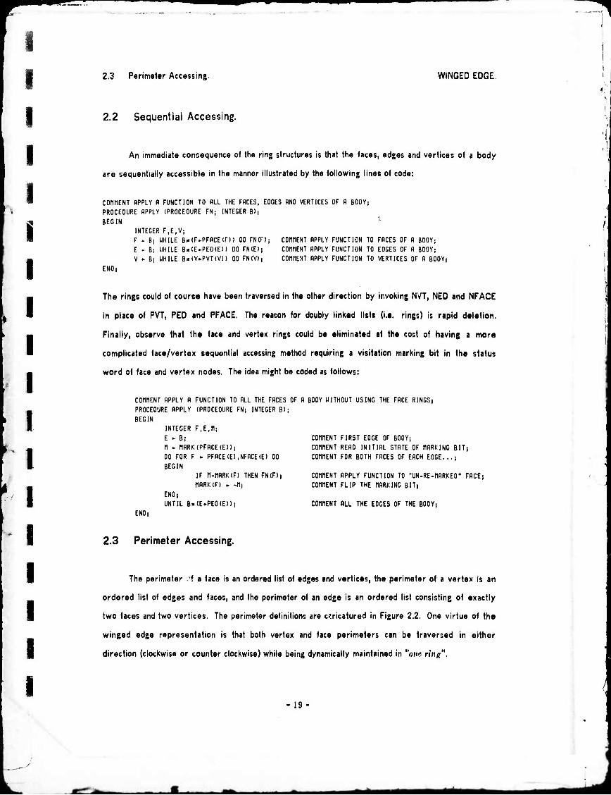
An immediate consequence of the ring structures is thai the faces, edges and vertices of a body
are sequentially accessible in the manner illustrated by the following lines of code:
COntlENT APPLY fl FUNCTION TO ALL THE FACES, EDGES AND VERTICES OF A BODY; PROCEDURE APPLY (PROCEDURE FNj INTEGER Bh BEGIN
INTEGER F,E,V; F - B) WHILE B-CF-PFACEID) DO FNlDj CDMtlENT APPLY FUNCTION TO FACES OF A BODY; E ► B; WHILE B«(E*PEO(E)) DO FN(E)| COtinENT APPLY FUNCTION TO EDGES OF A BODY; V - B; WHILE B«(V-PVTtV)) DO FN(V)) COHMENT APPLY FUNCTION TO VERTICES OF A BODY;
END;
The rings could of course have been traversed in the other direction by invoking Nv'T, NED and NFACE
in place of PVT, RED and PFACE. The reason for doubly linked list* (i.e. rings) is rapid deletion,
Finally, observe that the face and vertex rings could be eliminated at the cost of having a more
complicated face/vertex sequential accessing method requiring a visitation marking bit in the status
word of face and vertex nodes. The idea might be coded as follows:
COMMENT APPLY A FUNCTION TO ALL THE FACES OF A BODY WITHOUT USING THE FACE RINGS; PROCEDURE APPLY (PROCEDURE FN; INTEGER B); BEGIN
END;
INTEGER F.E.M; E . B; ft * MRRMPFRCECE)); DO FOR F - PFACE(E),NFACE(E) DO BEGIN
IF n=nARt;(F) THEN FN(F))
HfiRMF) ► -M;
END; UNTIL B.(E-PE0(E))|
2.3 Perimeter Accessing.
COMMENT FIRST EDGE OF BODY; COMMENT READ INITIAL STATE OF HARKING BIT; COMMENT FOR BOTH FACES OF EACH EDGE..,;
COMMENT APPLY FUNCTION TO "UN-RE-MARKED" FACE; COMMENT FLIP THE MARKING BIT;
COMMENT ALL THE EDGES OF THE BODY;
I
The perimeter i'f a face is an ordered list of edges and vertices, the perimeter of a vertex is an
ordered list of edges and faces, and the perimeter of an edge is an ordered list consisting of exactly
two faces and two vertices. The perimeter definitions are caricatured in Figure 2.2. One virtue of the
winged edge representation is that both vertex and face perimeters can be traversed in either
direction (clockwise or counter clockwise) while being dynamically maintained in "our ring".
19-

^^
2.3 Perimeter Accessing. WINGED EDGE.
FIGURE 2.2 - Three Kinds of Perimeters. 0
EDGE
A Vertex is surrounded by Edges and Faces
An Edge is surrounded by Faces and Vertices
A Face is surrounded by Edges and Vertices
Given one edge of a face (or vertex) perimeter, the next edge clockwise (or counter clockwise)
from the given edge about the particular face (or vertex) can be retrieved from the data structure
with the assistance of two subroutines called ECW and ECCW. The idea of the edge clocking routines is
to match the given face (or vertex) with one of the faces (or vertices) of the given edge and to then
return the appropriate wing. A possible coding of ECCW and ECW might be as follows:
COflMENT FETCH EDGE CCW FROfl E RBOUT FV; INTEGER PROCEDURE ECCU (INTEGER E.FV)! BEGIN "ECCW"
IF PFflCE(E)=FV THEN RETURN(PCCU (E))j IF NF3CE(E)=FV THEN RETURN(NCCW(E)I; IF PVT(E)=FV THEN RETURN(PCU(E)); IF NVT(E).FV THEN RETURN(NCW(E))i FflTflLj
END "ECCU"i
COriHENT FETCH EDGE CLOCKWISE FROfl E RBOUT FV| INTEGER PROCEOURE ECW (INTEGER E,FV)) BEGIN "ECW"
IF PFBCE(E)=FV THEN RETURN(PCW(E))) IF NFflCE(E)=FV THEN RETURN (NCW (E)) j IF PVT(E).FV THEN RETURN(NCCU(E)); IF NVT(E).FV THEN RETURN(PCCU(E))i FflTBLi
END "ECU")
The first edge of a face or vertex is (of course) immediately available from the PED field of the face or
vertex. For example, the two procedures below can be used to visit all the edges of ■ face or all the
edges of a vertex, respectively.
COWIENT BPPLY FUNCTION TO EDGES OF R FACE; PROCEDURE RPPLY (PROCEDURE FN; INTEGER F); BEGIN
INTEGER E,E0; E»E0>PED(F)i 00 FN(E) UNTIL E8.(E.ECCU(E,F))i
END;
COrtMENT APPLY FUNCTION TO EDGES OF fl VERTEXt PROCEDURE RPPLY (PROCEDURE FN) INTEGER V) ( BEGIN
INTEGER E.EO) E-EIKPEOW)) DO FN(E) UNTIL E8.(E-ECCW(E,V))(
END)
Using the same idea as in the edge clocking routines, a face or vertex can be retrieved relative
to a given edge and a given face or vertex. These routines include: FCW and FCCW which return the
/
20
^^ta
*m
2.4 Basic Polyhedron Synthesis. WINGED EDGF
face clockwise or counter clockwise from a given edge with respect to a given vertex; VCW and VCCW
which return the vertex clockwise or counter clockwise from a given edge with respect to a given
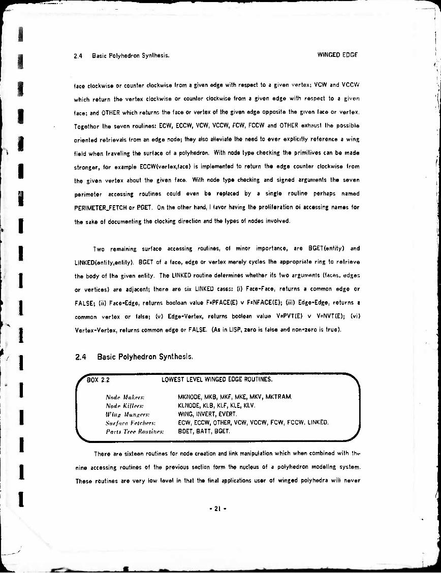
face; and OTHER which returns the face or vertex of the given edge opposite the given face or vertex.
Together the seven routines: ECW, ECCW, VCW, VCCW, FCW, FCCW and OTHER exhaust the possible
oriented retrievals from an edge node; they also alleviate the need to ever explicitly reference a wing
field when traveling the surface of a polyhedron. With node type checking the primitives can be made
stronger, for example ECCW(vertex,face) is implemented to return the edge counter clockwise from
the given vertex about the given face. With node type checking and signed arguments the seven
perimeter accessing routines could even be replaced by a single routine perhaps named
PERIMETER.FETCH or PGET. On the other hand, I favor having the proliferation 0» accessing names for
the sake of documenting the clocking direction and the types of nodes involved.
Two remaining surface accessing routines, of minor importance, are BGET(entity) and
LINKED(entity,entity). BGET of a face, edge or vertex merely cycles the appropriate ring to retrieve
the body of the given entity. The LINKED routine determines whether its two arguments (faces, edges
or vertices) are adjacent; there are six LINKED cases: (i) Face-Face, returns a common edge or
FALSE; (ii) Face-Edge, returns boolean value FsPFACE(E) v F»NFACE(E); (iii) Edge-Edge, returns a
common vertex or false; (v) Edge-Vertex, returns boolean value VaPVT(E) v V=NVT{E); (vi)
Vertex-Vertex, returns common edge or FALSE. (As in LISP, zero is false and non-zero is true).
2.4 Basic Polyhedron Synthesis.
BOX 2.2
Nodr Makrm:
Nodo Killers:
Wing MunRfrs: Surfaco. Frtrlwrit:
Parts Tree Routines:
LOWEST LEVEL WINGED EDGE ROUTINES.
MKNODE, MKB, MKF, MKE, MKV, MKTRAM.
KLNODE, KLB, KLF, KLE, KLV.
WING, INVERT, EVERT.
ECW, ECCW, OTHER, VCW, VCCW, FCW, FCCW. LINKED.
BDET, BATT, BGET.
"N
There are sixteen routines for node creation and link manipulation which when combined with the
nine accessing routines of the previous section form the nucleus of a polyhedron modeling system.
These routines are very low level in that the final applications user of winged polyhedra will never
21
^^
m^m
2.4 Basic Polyhedron Synthesis. WINGED EDGE.
explicitly need to make a node or mung a link. The word mung (meaning to modify an existing
structure by altering links in place) is LISP slang that deserves to be promoted into the technical
jargon; traditionally, a mung routine is one which makes applications of the LISP primitives RPLACA and
RPLACD. The twenty five routines listed in Box 2.2 are the bedrock foundation for the Euler
primitives presented in Chapter 3.
Node Makers and Killfn. The MKNODE and KLNODE are the raw storage allocation routines
which fetch or return a node from the available free storage. Tha MKB routine creates a body node
with empty face, edge and vertex rings; the body is placed into the body ring of the world model. The
MKF, MKE and MKV each take one argument and create a new face, edge or vertex node in the ring of
the given entity; with type checking these three primitives could be consolidated. Finally the MKTRAM
node creates a (mm node, which consists of twelve real numbers that represent either a Euclidean
transformation or a Cartesian frame of reference depending on the context. (Tram nodes are explained
in Section 3.3.) The corresponding kill routines KLB, KLF, KLE and KLV remove the entity from its
respective ring and return its node to free storage.
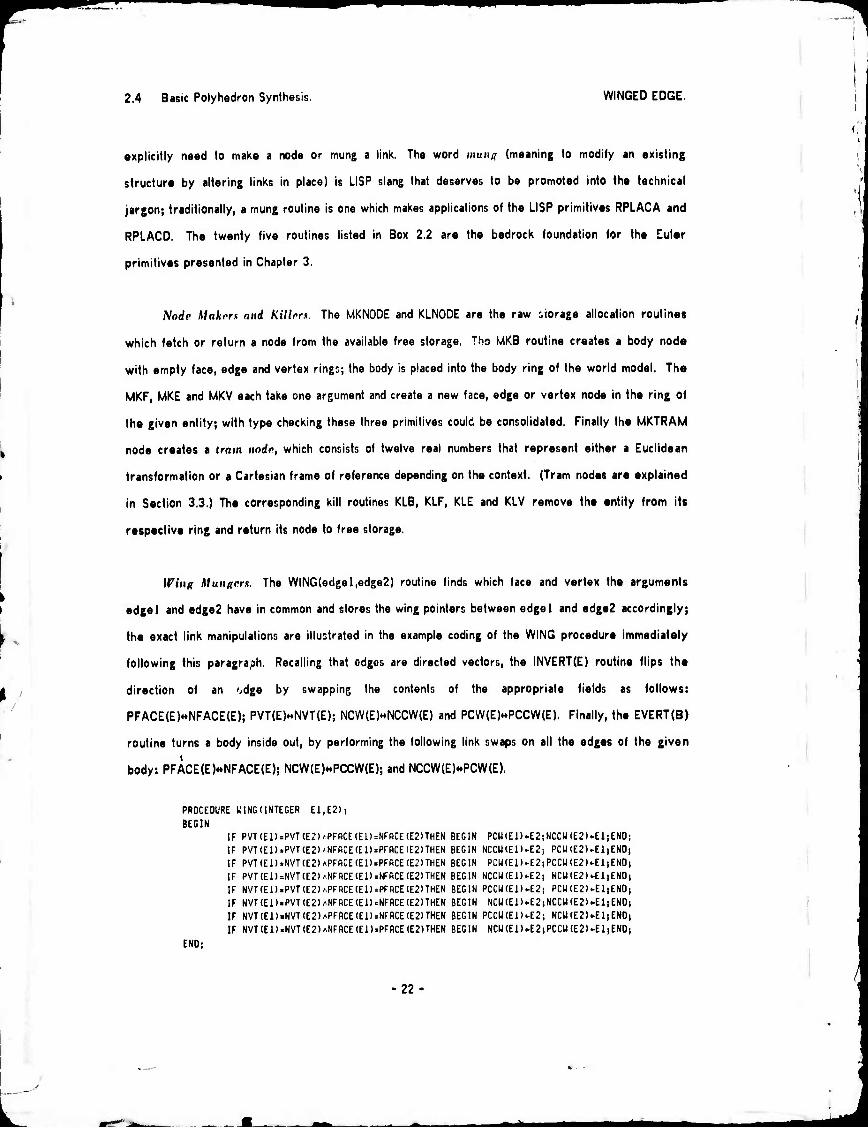
Ifing Mungfirs. The WING(edgel,edge2) routine finds which face and vertex the arguments
edgel and edge2 have in common and stores the wing pointers between edgel and edge2 accordingly;
the exact link manipulations are illustrated in the example coding of the WING procedure immediately
following this paragraph. Recalling that odgos are directed vectors, the INVERT(E) routine flips the
direction of an odge by swapping the contents of the appropriate fields as follows:
PFACE(E)«NFACE(E); PVT(E)«NVT(E); NCW(E)«NCCW(E) and PCW(E)HPCCW(E). Finally, the EVERT(B)
routine turns a body inside out, by performing the following link swaps on all the edges of the given
body: PFACE(E)«NFACE(E); NCW(E)*.PCCW(E); and NCCW(E)«PCW(E).
PROCEDURE ICING (INTEGER E1,E2)|
BEGIN IF PVT(E1)=PVT(E2)APFRCE
IF PVT(El).PVT(E2)/NFfiCE IF PVT(El).NVT(E2)APFfl:E IF PVT(El)=NVT(E2)ANFflCE IF NVT(E1).PVT(E2)APFBCE
IF NVT(El).PVT(E2)ANFflCE IF NVT(El).NVT(E2)APFflCE IF NVT(El).NVT(E2)ANFflCE
END;
(E1UNFBCE (EDrPFflCE (EUrPFflCE (El)=NFfiCE (El).PFflCE (EDsNFflCE (ElUNFRCE (El).PFflCE
(E2)THEN (E2)THEN (E2)THEN (E2)THEN (E2)THEN (E2)THEN (E2)THEN (E2)THEN
BEGIN BEGIN BEGIN BEGIN BEGIN BEGIN BEGIN BEGIN
PCW(El). NCCU(El). PCM(El).
NCCW(El). PCCU(El). NCU(E1)<
PCCinEl). NCU(E1)<
E2;NCCU(E2). E2) PCU(E2). E2;PCCH(E2). 12; NCU(E2)< E2; PCU(E2). E2!NCCU(E2)I
■E2; NCU(E2)< E2)PCCU(E2)(
EliENO; EljENO; E1|END( EljENOj EliENDj EliENO) EliENDi E1|EN0|
22- /
■ ü

^^
I f I I I I I
2.4 Edge and Face Splitting. WINGED EDGE.
Par» Tree Hautims. As mentioned before, body nodes can be grouped into a tree structure or
parts. The parts tree consumes four link positions (DAD, SON, BRO, SIS) and is maintained in body
nodes by the following primitives: BDET{body) detachs a body node from the parts tree,
BATT(bodyl,body2) attaehs bodyl to the ring of children belonging to body2, and BGET(imtily) returns
the body node at the head of the given face, edge or vertex ring. The SON field of a body may contain
a pointer to a headless ring of subpart bodies, the ring of subparts is maintained in the BRO (brother)
and SIS (sister) fields, and each subpart contains a pointer back to its parent in its DAD field. At
present, the notion of a body is coincident with the notion of a connected polyhedron; however by
allowing several bodies to be associated with a single polyhedral surface, a flexible object such as an
animal could be represented.
2.4 Edge and Face Splitting.
One of the most important properties of the winged edge representation is thai edges and faces
can be split using subroutines that make only local alterations to the data structure; and the splits can
easily be removed (since the doubly linked rings allow rapid deletion of nodes from a body). The edge
split routine, ESPLIT, makes a new edge and a new vertex and places them into the surface topology as
shown in Figure 2.3; the kill edge-vertex routine, KLEV, undoes an ESPLIT. The face split routine,
MKFE, creates a new edge and a new face and places them into the surface topology as shown in
Figure 2.4; the kill face-edge routine, KLFE, undoes a MKFE.
The rest of this section concerns implementation; it may be skipped by the applications oriented
reader. The split and kill routines are examples of a pattern which applies to the coding of operators
that alter winged edge structures. In a typical situation, there are five steps: first, get the proper
kinds of nodes into the body rings using the MKF, MKE, MKV primitives; second, position the vertices
by setting their XWC, YWC, 2WC fields; third, connect each vertex and face to one of its edges by
setting face/vertex PED fields; fourth, connect each edge to its two faces and its two vertices by
setting the NFACE, PFACE, NVT, PVT fields of the edge; finally, set up the wing perimeter pointers by
applying the WING primitive to the pairs of edges to be mated.
23-

^^»f
2.4 Edge and Face Splitting. WINGED EDGE.
I I
FIGURE 2.3 - ESPLIT AND KLEV.
.
BEFORE: VNEW •- ESPLIT(EDGE); AFTER: EDGE «- KLEV(VNEW);
INTEGER PROCEDURE ESPLIT (INTEGER E0GE>i BEGIN "ESPLIT"
INTEGER VNEH.ENEUi
COfWENT CREATE fl NEU EDGE AND VERTEX;
VNEH ► lirV(PVT(EOCE))j
ENEU - nKE(EDCE)i
COnnENT CONNECT VERTICES « FACES TO EDGES;
PVT(ENEU) ► PVT(EOCE); NVTCENEll) ► VNEll;
PVT(EDGE) ► VNE1J-,
PFACEfENEU) - PFACE(EDGE);
NFACECENEU) * NFflCE (EDGE);
COflHENT CONNECT EDGES TO VERTICES;
IF PED(PVT(EDCE)=EDCE THEN
PED(PVT(EDGE))-ENEWi
PED(VNEU)^ENEU;
COtWENT LINK THE WINGS TOGETHER)
NCU(ENEU) . EDGE-, PCCW(ENEU) » EDGE;
PCU(EDGE) - ENEU; PCCU(EDGE) - ENEU)
UINC(NCCU(EDGE),ENEU)i
UING(PCU(EDGE),ENEU);
RETURN(VNEU)|
END "ESPLIT"|
AFTER: VNEW *■ ESPLIT{EDGE); BEFORE: EDGE ♦■ KLEV(VNEW);
INTEGER PROCEDURE rLEV (INTEGER VNEU);
BEGIN "KLEV"
INTEGER EDGE,ENEU(V,F,B;
ENEU ► PEG(VNEU); EDGE ► ECCUIENEU.VNEU);
COnnENT ORIENT EDGES AS IN DIAGRAM;
IF NVT(ENEU) « VNEU THEN INVERT (ENEU);
IF PVT(EDGE) « VNEU THEN INVERT(EDGE);
COfUIENT TIE E TO ITS NEU UPPER VERTEX RND UINCSi
V - PVT(EDGE) ► PVT(ENEU)) UING(PCU(ENEU),EDGE);
UING(NCCU(ENEU),EDGE)!
COnnENT ELIMINATE OCCURRENCES OF ENEU IN F AND V|
IF PEO(V)rENEU THEN PED(V) * EDGE
IF PED(PFACE(EDGE))=ENEU THEN
PED(PFACE(EDGE))-EOGE|
IF PED(NFACE(EOGE))=ENEU THEN
PED(NFACE(EDGE))-EDCE;
COnnENT REMOVE NODES FROM RINGS AND RETURN EDGE)
KLV(VNEU)|
KLE(ENEU)|
RETURN(EDGE)|
END "KLEV"i
I
Th« actual routines differ slightly from those given above in that they do argument type
checking and data structure cheeking; nevertheless, a diagnostic trace of the implemented version
reveals that the ESPLIT routine executes an average of 170 POP-10 instructions and the KLEV routine
executes an average of 200 instructions.
24-
i I I I I /

^^
i
I I
2.4 Edge and Face Splitting. WINGED EDGE.
FIGURE 2.4 - MKFE AND KLFE.
BEFORE: ENEW AFTER: FACE
MKFE(V1,FACE,V2)} KLFE(ENEW);
AFTER: ENEW ♦ BEFORE: FACE
MKFE(V1,FACE,V2); - KLFE(ENEW);
I I I I I I I I I I
INTEGER PROCEDURE WFE (INTEGER Vl,FflCE,V2) i
BEGIN "nt-FE" INTEGER Vl.V^FNEU.ENEII.E.EO.B.V;
COnnENT CREPTE NEU FACE S EOCEi
FNEU - nr.F(FRCE): ENEW > Mt E (PEO(FRCE));
COmiENT LINK NEU EDGES TO ITS FACES S VERTICESj
PEO(F) - PED(FNEU) ► ENEllj
PFRCE(ENEIJ> ' F; NFfiCE(ENElJ) ► FNEMi
PVT(ENEW) . VI; NVT(ENEU) ► V2i
COnnENT GET THE WINGS OF THE NEU EDGE;
E2 ► PEOIVD)
DO E2-ECW((E1*E2))V1) UNTIL FCU(El,Vl)=FflCEi
E4 ► PEDIVDi
DO E4>ECW((E3^E4),V2) UNTIL FCU(E3)V2).FBCEi
COnnENT SCAN CCU FROn VI REPLACING F'S WITH FNEW|
E - E2;
DO IF PFACE(E)=FRCE THEN PFRCE(E)^FNEM
ELSE NFRCE(E)>FNEUi
UNTIL E4 = (E-ECCtnE.FNEU));
COnnENT LINK THE WlNGSj
UlNGtEl.ENEUh WING (E2,ENEW);
UING(E3,ENEU); UING(E4,ENEU);
RETURN(ENEHIj
ENOs
INTEGER PROCEDURE KLFE (INTEGER ENEW);
BEGIN "KLFE"
INTEGER FNEH,FBCE.Vl1V2,E,Ei,E2,E3,E4i
COtltlENT PICKUP ALL THE LINKS OF ENEII;
FACE * PFACE(ENEU); FNEU - NFfiCE(ENEU)i
VI * PVT(ENEU)i V2 ► NVT(ENEU)i
El ► PCU(ENEU)i £2 * NCCU{ENEU)i
E3 - NCU(ENEU); E4 * PCCtl(ENEU);
COtlflENT GET ENEW LINKS OUT OF FACE, VI AND V2t
IF PED(Vl) = ENEU THEN PED(Vl) ► El)
IF PED(V2) = ENEW THEN PED(V2) - E3;
IF PED(FACE)=ENEU THEN PEO (FACEUES;
COnnENT GET RID OF FNEU APPEARANCES;
E * E2)
DO IF PFACE(E)=FNEH THEN PFACE (E)^ACE
ELSE NFACE(E)-FACE;
UNTIL E4 • (E.-ECCU(E,FNEU));
COIKIENT LINK WINGS TOGETHER ABOUT FACE;
UINC(E2,E1);UING(E4IE3)! KLF(FNEW)jKLE(ENEH!i
RETURN(FACE)|
END)
Again, the actual routines differ from those given above in that they do argument type checking
and data structure checking. The above two routines typically take about twice as long to execute as
the previous pair; notice that the execution time is dependent on the length of face perim. ters, which
are mostly three or four edges long.
25
/
^rih

^^m-
2.5 Coordinate Free Polyhedron Representation. WINGED EDGE.
2.5 Coordinate Free Polyhedron Representation.
As in general relativity, all goomotric entities can be represented in a coordinate free form. In
particular, the vertex coordinates of a polyhedron can be recovered from edge lengths and dihedral
angles (the angle formed by the two faces at each edge). Having the geometry carried by only two
numbers per edge rather than by three numbers per vertex does not necessarily yield a more concise
representation because edges always outnumber vertices two for one, and in the case of • triangulated
polyhedron edges outnumber vertices by three to one.
One application of a coordinate free representation arises when it is necessary to measure a
•hap« with simple tools such as a caliper and straight edge. For example, one way to so «bout
recording the topology and geometry of an arbitrary object is to draw a triangulated polyhedron on its
surface with serial numbered vertices and to record for each edge its length, its two vertices and its
»igmi dihedral length. The dihedral length is the distance between the vertices opposite the edge in
each of the edge's two triangles; the length can be given a sign convention to indicate whether the
edge is concave or convex. The required dihedral angles can then be computed from the signed
dihedral lengths.
I I I
1 .
.
26
*mm ■■I ^^__—I *mm

■P9W
3.0 Iniroduction to GEOMED. GEOMED.
I I
1
SECTION 3.
A GEOMETRIC MODELING SYSTEM.
3.0 Introduction to GEOMED. 3.1 Euler Primitives. 3.2 Routines using Euler Primitives.
3.3 Euclidean Routines. 3.4 Image Synthesis: Perspective Projection and Clipping.
3.5 Image Analysis: Interface to CRE.
3.0 Introduction to GEOMED.
I
1 I
I
GEOMED (Geometric Editor) is a system ot subroutines for manipulating winged edge polyhedra.
The system has two manifestations: first, it appears as an interactive 3-D drawing program and second,
it appears as a geometric modeling command language. It is the latter manifestation along with some of
the details of implementation that is the subject of this chapter; the interactive drawing program is
documented in (Baumgart 74). As a language, GEOMED is all semantics with no particular syntax of its
own; there are about two hundred subroutines which take from zero to four arguments, return one or
no values and which usually have considerable side effects on the data structures. The subroutines can
be grouped into five classes: utility routines, Euler routines, Euclidean routines, image synthesis and
image analysis routines. The utility routines include input/output, trigonometric functions, memory
management, a command scanner, and device dependent display routines; the utility routines will not be
further elaborated. The Euler routines perform topological operations on links, the Euclidean routines
perform geometric computations on data, and the image synthesis routines perform photographic
simulations on the model as a whole. The fifth class, image analysis routines, consists at present solely
27
mmm
3.0 Introduction to GEOMED. GE0ME0.
of an inUrfac« between GEOMED and CRE, the fifth group lacks the completeness of the other parts of
the system.
As in the previous chapter, the programming notation used will continue to have an ALGOL
appearance with specific examples of actual GEOMED code being given in the language SAIL (Stanford
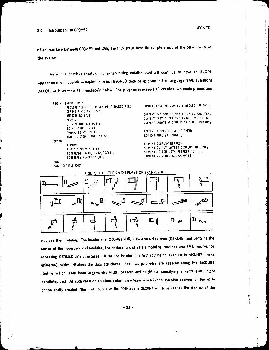
ALGOL) as is ex'mple «1 immediately below. The program in example »1 creates two cubic prisms and
BEGIN "EXfiUPLE ONE" REQUIRE ■'GEOnES.HORtCEn.HEr SOURCEJILE]
DEFINE PI."3.14159:7";
INTEGER 81,62,11 tlKUNIV; Bl * MfCUBE(8,l,0.S);
B2 ► nrCUBE(1,2,4)) TRflNSL(82,-7,1.5,01;
FOR 1-1 STEP 1 THRU 24 DO
BEGIN CEODPYi PL0T0("TnP."«CVS(l)); ROTATE(81,PI/18,PI/12,PI/13);
R0TRTE(B2,8,2*PI/23,8)I
END; END "EXBriPLE ONE";
COhnENT DECLRRE CEOnED ErtBEDOEO IN SRIL;
COnnENT TWO BODIES RNO RN IHRGE COUNTER; COnnENT INITIRLIZE THE DRTR STRUCTURES;
COmENT CRERTE fl COUPLE OF CUBIC PRISHSi
COHMENT DISPLRCE ONE OF THEfl;
COMMENT MRICE 24 HIRCES;
COMMENT DISPLRY REFRESH; COMMENT OUTPUT LATEST DISPLAY TO DIStC; COMMENT RCTION WITH RESPECT TO ...;
COMMENT ...WORLD COORDINRTES;
FIGURE 3.1 - THE 24 DISPLAYS OF EXAMPLE «1
Qt 0 c^ ^ 7 V V
,01 •^0
a si m JCD ^^D
DJI O ID <P
displays them rotating. The header file, GEOMES.HDR, is kept on a disk area [GEM.HE] and contains the
names of the necessary load modules, the declarations of all the modeling routines and SAIL mscros for
accessing GEOMED data structures. After the header, the first routine to execute is MKUNIV (make
universe), which initializes the data structures. Next two polyhedra are created using the MKCUBE
routine which takes three arguments: width, breadth and height for specifying a rectangular right
parallelepiped. All such creation routines return an integer which is the machine address of the node
of the entity created. The first routine of the FOR-loop is GEODPY which refreshes the display of the
28 /

^^"T
I I I I i I
3.0 Introduction to GEOMED. GEOMED.
I I
model. Finally, the example calls TRANSL and ROTATE which perform translation and rotation. TRANSL
takes four argument: the thing to be moved followed by the three components of a translation vector;
similarly ROTATE takes four arguments: the thing to be moved followed by the three components of a
rotation vector; there are several other ways to specify translation and rotation.
FIGURE 3.2 - THE 24 DISPLAYS OF EXAMPLE «2.
BEGIN "EXfltlPLE TUO" REQUIRE "CCOMfS.HDRtGEfl.HE]" SOURCEJILEi
DEFINE ox"C0MI1ENT"i DEFINE PI."3,1*15927"; INTEGER B1,B:,J1,J2,J3,J4,J51J61C1,CHR,1!
riKUNIV|GEODPV;
Bl - INR3D("RRI1[DRT,BCBl")i B2 ► INR30("TflBLEtDflT,BGBr)| Jl ► FONntlECJOINTDj J2 « FDNflnE("J0INT2"); J3 ► FDNRME("JOINTS")i J4 ► FONflNE("JOINT«"); J5 ► FDNflnE("JOINTS")| J6 ► FDNfiME("JOINTS"!; Cl
o GEOMED EMBEDDED IN SRILi a DECLARE COMMENT PREFIXj
o MODEL OF THE YELLOU RRMi a MODEL OF THE HRNO/EYE TRBLti a SHOULDER - RBOUT VERTICAL) a RRM - ABOUT HORIZONTAL; a SLIDE; a WRIST TUIST; a WRIST FLAP; a HAND;
INCRMC'RRMCRMtDAT.BGB)"); a INPUT A PRRTICULRR CRMERR MODEL; a TWENTY FOUR IMRGES FOR FIGURE 3.2;
a HIDDEN LINE ELIMINRTION OISPLRY REFRESH; a OUTPUT LATEST DISPLAY FILE TO DISK; a ACTION WITH RESPECT TO BODY COORDINRTES. , a ...WHEN BODY ARGUMENT IS GIVEN NEGATIVE;
FOR M STEP 1 UNTIL 24 DO BEGIN
SH01I2(0,0); PLOTO("PLTx:."SCVS(I)); R0TRTE(-J1,0,0,PI/40);
R0TRTE(-J2,0,0,-PI/SO); TRANSL(-J3,0,0,0.06);
END; END "EXAMPLE TWO";
In example «2, the model of an actual robot arm is read in and the first three joints are run
through a simulated arm motion. The routine INB30 reads a B3D polyhedron file from the disk. The
arm was drawn from measurements using the interactive form of GEOMED. The FDNAME, find name,
routine retrieves a body by its print name; FDNAME returns zero when a name is not found. The
routine INCAM reads in a camera file. Finally, the routine SHOW2 calls the hidden line eliminator;
when SHOW2,s arguments are zero, default options are assumed. The arm model was originally made
29 -
^fe mm

^m^
3.1 Euler Primitives. GEOMED.
to illustrate an arm trajectory for a thesis on arm control (Paul 69) and has been used two times since
in projects concerning arm trajectory planning and arm collision avoidance.
GEOMED is a hierarcy ot several levels of routines that are finally invoked by syntactically trivial
subroutine calls. The point illustrated by the examples is that some applications level GEOMED cod«
has a quite ordinary appearance that does not require mastery of the many underlying primitives which
are explained in the next several sections.
3.1 Euler Primitives.
The Euler routines are based on the idea that an arbitrary polyhedron can be created in steps
that always maintain the Euler relation: F-E.VS2*IB-H). Topologically, a connected Eulerian polyhedrai
graph can be built up with only lour creation primitives: MKBFV, MKEV, MKFE and GLUEE or taken
apart with four kill primitives: KLBFEV, KLEV, KLFE and UNGLUEE. The prefixes "MK" and "KL", stand
for make and kill; the initials "B", "F", "E" and "V" invariably stand for body, face. cdKr and vertex
and tend to appear in that order. The notion of GLUE is associated with the process of forming (or
removing) a handle which increases (or decreases) the topological genus of the surface by on* unit.
Th« MKBFV primitive takes no arguments and creates a degenerate point polyhedron of one vertex,
or.* face and one body which is the minimal non-zero binding satisfying the Euler relation. The MKEV
creates a new edge and a new vertex, the new edge is attached to the old vertex as a spur in the
perimeter of the given face. The MKFE creates a new face and a new edge, the new edge is placed
between the two given vertices. And the GLUEE routine creates a handle or kills a body node by
placing a new edge between two given vertices and by removing the second of two given faces.
Completing the set, the ESPL1T routine (explained in Section 2.5) is included as a form of MKEV.
In principle, the advantages of the pure Euler primitives are that they assure valid topology, full
generality, reasonable simplicity and they achieve a semantic level slightly higher than that of
manipulating the nodes and links directly. However, the Euler primitives only satisfy the first of the
conditions defining a solid polyhedron; imposing no particular restrictions on surface orientation,
face/vertex trivalence, face planarity, face convexity or surface self intersection. Furthermore, even
-30-
1 I
;
!
i i
^**

mmm
3.1 Euler Primitives. GCOMED
some low level lopologieal operations (such as body intersection, Chapter 5) are inconvenient to
specify in term of the Euler primitives. Nevertheless in practice, the Euler primitives perform a useful
role as a topological foundation for coding routines which embody more algebra and geometry and
which lead to higher semantic levels.
<B0x 3.1 THE EULER PRIMITIVES. "V
EULER MAKE PRIMITIVES:
I. BNEW«-MKBFV; Makes point polyhedron.
2. VNEW f MKEV(F,V); Makes new edge and vertex.
VNEW *■ ESPLIKE); Makes new edge and vertex.
3. ENEW-MKFE(V1,F,V2); Makes new face and edge.
4. ENEW-GLUEE(F1,V1,F21V2); Makes new edge, kills F2,
and makes a hole or kills a body,
EULER KILL PRIMITIVES: 1. QNEW ♦-KLBFEV(Q); Kills bodies, faces, edge and vertices.
2. FACE •■ KLFE(E); Kills E and NFACE(E). Returns PFACE(E).
3. EDGE «- KLEV(V); Kills V and PED(V). Returns other E of V.
VERT - KLEV{E); Kills E and NVT(E). Returns PVT(E).
4. FNEW - UNGLUE(E); Kills E, makes F. Returns the new face.
^
and kills a hole or makes a body. /
The remainder of this section consists of more explanation and examples of the Euler primitives
and may be skipped by the reader who does not need an elaboration of this level of modeling.
Noit-mlid »olyhrdrn: Intermediate between Eulerian and solid polyhedra are the wire, dangling-wire
(or spur), lamina, sheet and wasp-edged polyhedra which are transition states for creating and altering
polyhedral solids. The wirr polyhedron consists of one face, N edges and N«l vertices. A Inmiun is a
two faced polyhedron with no interior edges or dangling wire. A dnngling wirr or spur is made when
a MKEV is applied to a vertex of an already closed simply connected face perimeter; dangling wire
spurs are ultimately "closed" or "tied down" by a MKFE application. A thrrt is an array of lamina, with
the exception of ruled surfaces of rotation, commands for folding and manipulating sheets have not
been developed. Finally, a wasp polyhedron is a transition stale formed by the GLUEE primitive; this
degenerate polyhedron is named for the wasp waisted face perimeter which (like a spur) is eliminated
by appropriate MKFE applications.
31
-■^
^^^r-
3.1 Eular Primitives. GEOMED.
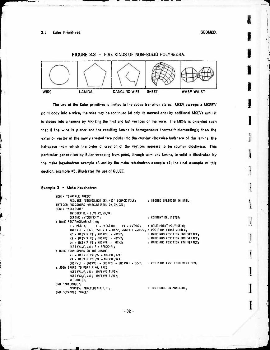
FIGURE 3.3 - FIVE KINDS OF NON-SOLID POLYHEDRA.
WIRE LAMINA DANGLING WIRE SHEET WASP WAIST
The use of the Euler primitives is limited to the above transition states. MKEV sweeps a MKBFV
point body into a wire, the wire may be continued (at only its newest end) by additional MKEVs until it
is closed into a lamina by MKFEing the first and last vertices of the wire. The MKFE ic oriented such
that if the wire is planar and the resulting lamina is homogeneous (non-self-intersecting); then the
exterior vector of the newly created face points into the counter clockwise halfspace of the lamina, the
halfspace from which the order of creation of the vertices appears to be counter clockwise. This
particular generation by Euler sweeping from point, through wir' and lamina, to solid is illustrated by
the make hexahedron example *3 and by the make tetrahedron example «4; the final example of this
section, example «5, illustrates the use of GLUEE.
Example 3 - Make Hexahedron.
BEGIN "EXRHPLE THREE" REQUIRE "GEOIIES.HDRlCEn.HEl" SOURCEJILEI
INTEGER PROCEDURE IWKECUBE(REftL DX.DY.DZli BEGIN "imECURf"
INTEGER B,r>E>Vl)V2,V3,V4) DEFINE »."COrmENT"!
a HAKE RECTRNCULRR LfiMINfi; B <- tlKBFV; F^PFflCE(B)i Vl*PVT(B)i XUC(Vl) .. DX/2J VUCtVl) - 0Y/2i ZUC(Vl) —DZ/2| V2 ► nKEV(FIVl)i XUC(V2) ► -DX/2) V3 ► nKEV(F,V2)j YUC(V3) - -DY/2; V4 ► OKEVtF.VS)! XHC(V4) ► 0X/2| HKFEm.F.V*)) F ► PFflCE(F)j
a HAKE FOUR SPURS ON THE LRIHNRt VI ► nr.EV(F,Vl)|V2 ► nKEV(F>V2)i V3 ► nKEV(F1V3);V4 . nKEV(F,V4); ZUC(Vl) k ZUC(V2) ► ZWC(V3) ► ZUC(V4) ► DZ/2j
a JOIN SPURS TO FORM FINAL FRCE; HKFE(V1,F,V2)| nKFE(V2>F,V3)i nKFE(V3,F,V*)) tnCFEM.F.Vl»! RETURN(B)|
END "nflKECUBE"; HKUNIV; HRKECUBE(16,8,6);
END "EXRHPLE THREE";
-32
a GEOMED EHBE0DE0 IN SRILj
a COnnENT 0ELII1ITER!
o (IRCE POINT POLYHDERfli a POSITION FIRST VERTEX| a nfiKE RND POSITION 2ND VERTEXj o nRKE RND POSITION 3RD VERTEXj a HRKE RNO POSITION 4TH VERTEX)
a POSITION LRST FOUR VERTICES)
o TEST CRLL ON HRKECUBE)
I I I !
i
I

I I I I
[
3.1 Euler Primitives.
Example 4 - Make Regular Tetrahedron.
BPGIN "EXRMPLE FOUR"
REQUIRE "CEOnES.KDRICEMEl" SOURCEJILE; DEFINE o."COmiENT"il)£FINE PI = "3.1415927";
INTEGER PROCEDURE ni'TETRfl (REfiL R); BEGIN "tllTETRB"
INTEGER B,Fl,F:,Vl,V2,V3,V4i B - niBFVj Fl - PFflCEIB); VI » PVT(B); WCm) ► BBS(R*0.342689)! tllC(Vl) ► -flBS(R/3)| V2 - HKEVCFl.Vlli R0TflTE(v:,0,0,2'/PI/3)j V3 - m:£V(Fl,V2)i ROTATE (73,0,O^^PI^); V4 ► f1(:EV(Fl,V3)i XIJC (V4) »YWC (V4) »0i ZUG (V4) ►BBS IR) i HKFE<V1,F1,V4)| F2 ► PFflCECFDj m:FE(Vl,Fl,V31 j m:FE (72^2,74)1
RETURN(Bl) END "nKTETRfl"i
mUNIVi l1KTETRfl(6)| GEODPY;
END "EXBMPLE FOUR")
Example 5 - Glue two N-edged faces together.
BEGIN "EXflMPLE FIVE" REQUIRE "GEOtlES,HÖRIGEM,HE!" SOURCEJILEj DEFINE !i="C0nnENT"; DEFINE PU"3.1415927"; INTEGER B1,B2!
INTEGER PROCEDURE GLUEFF(INTEGER FflCEl,FBCE2); BEGIN "GLUEFF"
INTEGER V,V1,V2,E,E0,I; REBL DniN.D; VI ► VCCU(PEO(FflCEl),FflCEl)|
a FIND VERTEX OF FflC£2 THAT IS CLOSEST TO Vl) OniN ► lOelO; E - £8 * PED(FflCE2)! DO BEGIN
V ► VCCII(E,FBCE2);0 ► DISTflN(Vl,V); IF D<0I1IN THEN BEGIN 0niN<-DlV2>ViEN0|
END UNTIL EO = (E»ECCW(E,FflCE2))i a nM.l THE HBSP EDGE;
E * CLUEE(FBCEl,Vl,FflCE2>V2); o CLOSE OTHER EDGES;
V * 0THER(NCCU(E),V1)) DO BEGIN
VI ► OTHER (PCIKE),VI)) V2 ► OTHER (PCCII(E),V2)i E ► m:FE(Vl>FflCEl(V2);
END UNTIL VrVl; RETURN(BGET(E)I;
END "GLUEFF"; ni-UNIV; Bl •■ tirCUBE(2,2,2); B2 > n^CUBEO.S.S); ROTATE(Bl.O,-PI/2,0);TRflNSL(81,-3,0,8); ROTATE (B2,8, ^1/2,0);TRnNSL(B2,*4,8,8); CLUEFF(PFACE(Bl),PFfiCE(B2)l; GEODPY;
END "EXflnPLE FIVE";
GEOMED.
o CEOtlED EriBEODED IN SAIL;
o IIBKE TETRAHEDRON;
a HAKE POINT POLYHOERR; a POSITION FIRST VERTE»; a MBCE AND POSITION 2ND VERTEX; a MALE AND POSITION 3RD VERTEX; a MAKE AND POSITION 4TH VERTEX;
a CLOSE Sr.EU QUADRILATERAL;
a RETURN THE CREATION;
a INITIALIZE AND TEST M^TETRfl; ot DISPLAY REFRESH;
a GEOMED EMBEDDED IN SAIL;
a TWO TEST CUBES; a DEMO CLUE FACE TO FClCE-
a PICK ONE VERTEX OF FACEl;
a INITIALIZE MINIMAL DISTANCE;
a SCAN FACE2 FOR VERTEX CLOSEST TO VI(
a FACE2 AND BODY ARE KILLED;
a LAST VERTEX, TO STOP SCAN;
a FETCH NEXT PAIR OF VERTICES;
a CLOSE AN EDGE;
a RETURN THE SURVIVING BODY;
a INITIALIZATION; a TUO TEST CUBES; a ORIENT CUBES SO FIRST FACES...; a ...ARE OPPOSITE; a TEST THE FUNCTION; a DISPLAY REFRESH;
33-
^rita

3.2 Routines using Euler Primitives. GEOMED.
3.2 Routines using Euier Primitives.
Further methods of polyhedral construction can readily be coded using the Euler primitives. For
example, the routines listed in Box 3.2 illustrate «he direct generation of simple prototypical polyhedra,
as well as contruction by sweeping, cutting, glueing, copying and duality.
BOX 3.2
1. BNEW
BNEW *■ BNEW *• FACE*-
FACE«- PEAK •-
7. BODY «- 8. BNEW ♦■ 9. QNEW •• 10. BODY «-
2.
3. 4.
5. 6.
ROUTINES USING EULER PRIMITIVES.
MKCUBE(DX,DY,DZ); Create right rectangular prism. MKCYLN(RADIUS,N(DZ)j Create cylinder approximation. MKBALL(RADIUS,M,N); Create sphere approximation.
Make prism on face (or sweep wire). Rotation sweep wire face completion. Make pyramid on a face (or vertex). Removes facel and face2. Divide body at cutting plane. Copy an entity. Apply face/vertex duality to a body.
SWEEP(FACE,FLAG); ROTCOM(FACE); PYRAMID(FV); GLUE(FACE1IFACE2); MKCUT(BODY,X,YIZ); MKCOPY(ENTITY);
FVDUAUBODY);
The first three routines make cubic prisms as well as polyhedral approximation« to circular
cylinders and spheres; or more accurately, MKCUBE creates rectangular right prisms, MKCYLN creates
regular polygonal right cylinders and MKBALL creates hedrons faceted by two N-sid#d regular polar
polygons and N«(M-1) trapezoidal polygons with all vertices lying on the surface of a sphere of a
given radius.
FIGURE 3.4 - Examples of MKCUBE, MKCYLN and MKBALL
MKCUBE Results MKCYLN Results MKBALL Results
Although, the implementation of curved edges and curved faces in GEOMED has always been
jusi around the corner, I have balked at the idea because it would require additional nodes connected
to edges and faces or it would require expanding the node size, which I have always before taken as
34
I
I I
I I
I I I
I I
I I I
I I
I I 1
- ^-
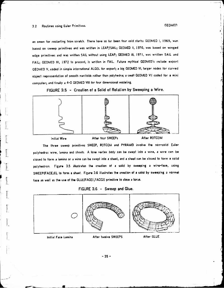
3.2 Routines using Euler Primitives. REOMFP
I
:
an omen for restarting from scratch. There have so far been four cold starts: GEOWED I, 1 969, was
based on sweep primitives and was written in LEAP/SAIL; GEOMED II, 1970, was based on winged
edge primitives and was written SAIL without using LEAP; GEOMED III, 1971, was written SAIL and
FAIL; GEOMED IV, 1972 to present, is written in FAIL. Future mythical GEOMED's include export
GEOMED V, coded in simple international ALGOL for export; a big GEOMED VI, larger nodes for curved
object representation of smooth manifolds rather than polyhedra; a small GEOMED VII coded for a mini
computer; and finally a 4-D GEOMED VIII for four dimensional modeling.
FIGURE 3.5 - Creation of a Solid of Rotation by Sweeping a Wire.
Initial Wire After four SWEEPs After ROTCOM
The three sweep primitives SWEEP, ROTCOM and PYRAMID involve the non-solid Euler
polyhedra: wire, lamina and sheets. A lone vertex body can be swept into a wire, a wire can be
closed to form a lamina or a wire can be swept into a sheet, and a sheet can be closed to form a solid
polyhedron. Figure 3.5 illustrates the creation of a solid by sweeping a wire-face, using
SWEEP(FACE,0), to form a sheet. Figure 3.6 illustrates the creation of • solid by sweeping a normal
face as well as the use of the GLUE(FACE1,FACE2) primitive to close a torus.
FIGURE 3.6 - Sweep and Glue.
O
Initial Face Lamina After twelve SWEEPS After GLUE
35

3.2 Routines using Euler Primitives. GEOMED.
Th« sweep flag argument determines whether triangles (flag non-zero) or rectangles (flag zero)
art to be formed as the sweep of the edges of the face. Sweeping out rectangles forms prisms,
sweeping out triangles forms prismoids. The PYRAMID routine when applied to a face creates a peak
vertex at the average locus of vertices of the Idee and connects all the vertices of the given face to
the peak vertex. PYRAMID applied to a vertex coorces all the faces of the vertex to be triangles, the
interpretation being that the given vertex is to be made like a peak of a pyramid. Prismoid sweep and
face pyramiding are illustrated by the construction of an icosahedron in Figure 37; the icosahedron can
be changed into a dodecahedron by the DUAL routine. The DUAL routine mungs face nodes into vertex
nodes and vertex nodes into face nodes; the new vertices are placed at the arithmetic mean of the
vertices of the old faces, consequently the dual is not its own inverse since objects tend to shrink.
FIGURES.? - ICOSAHEDRON BY PRISMOID SWEEP AND PYRAMID SWEEP.
The MKCUT(BODYlX,Y,Z) primitive divides a body at cutting plane into as many pieces as
necessary. Figure 3.8 illustrates how to cut a toroidal polyhedron into thirteen pieces using only three
cutting planes, after Figure 63 of (Gardner 61). The action of MKCOPY should be obvious - a new
polyhedron is returned that has the same topology, geometry and photometry as the given polyhedron.
More routines using Euler primitives could be coded for particular applications in architecture,
computer animation, mechanical design, numerical machine control, assembly diagraming and so on.
FIGURE 3.8 - THREE CUT TORUS DISSECTION INTO THIRTEEN PARTS.
I
I
36
I !
I I I I

3.3 Euclidean Routinas. GEOMFD
3.3 Euclidean Routines.
The Euclidean routines o< GEOMED fall roughly into four groups: transformations, metrics, tram
routines and space simulators. The Euclidean transformations are translation, rotation, dilation and
reflection following Klein's Erlangen Program, 1872. The Euclidean metric routines compute distances,
angles, areas, volumes and inertia tensors. The tram routines create or alter tram nodes which are the
main topic of this section. The final group of routines perform spatial simulations such as collision,
intersection, propinquity, occupancy and occultation.
Trnm \orlrs. A tram node contains twelve real numbers. Fundamental to all the Euclidean
routines is the curious fact that tram nodes have two interpretations: they may represent a cooHmate
system or they may represent a Euclidean transformation. As a coordinate system, the twelve number^
contain a location of the origin of the coordinate system as well as the three components of each of the
three unit vectors of the axes of the coordinate system. As a transformation, the application of a tram
node to a vertex is defined by the procedure named SCREW, given below.
Tram as a Coordinate System:
location of origin of coordinates:
components of X-axis unit vector:
components of Y-axis unit vector:
components of Z-axis unit vector:
7>nm Node Data I'irld Nama
XWC, YWC, ZWC, LOCATION VECTOR.
IX, IY, IZ,
JX, JY, JZ, ORIENTATION MATRIX.
KX, KY, KZ.
Tram as a Transformation: COnriENT RPPLY TRRfl Q TO VERTEX V POSTFIXj
PROCEDURE 3CREU (INTEGER V,Q);
BEGIN PERL t,y,Z;
X ► XUC(V); Y ► YUC(V), Z - ZUC(V)i
XUC(V) ► X«IX(Q) ♦ Y«JX(Q) ♦ 2«KX(Q) ♦ XUC(Q)i
YHC(V) * X«IY(Q) ♦ Y<.JY(Q) ♦ 2*KY(Q) ♦ YUC(Q)|
rUC(V) ► X*IZ(0) ♦ Y<.JZ(Q) ♦ ZtKZCQ) ♦ ZWC(0)i
END;
Generalizing, the procedure APTRAWIENTITY.TRAM) applies a tram to an arbitrary entity The
APTRAM procedure is formed by surrounding the SCREW procedure with suitable type checking and
data structure tracing mechanisms so that a tram can be applied (postfix) to almost anything:: bodies,
faces, edges, vertices, as well as to other trams, camera models and window nodes.
37
^rih imm

3.3 Euclidean Routines. GEOMED.
To repeat for emphasic, a tram node has two interpretations; a tram node may be interpreted as
a coordinate system and the very same tram node may be interpreted as a Euclidean transformation. A
source of confusion, is that a coordinate systom tram is a definition of one coordiate system (call it llv>
body coordinates) in terms of another coordinate system (call it the world coordinates). The application
of a body coordinate system tram to an en',:ty in body coordinates brings the entity down into the
world coordinate system in which the tram is defined. To say it another way, th« rule is that
APTRAM(BODY,TRAM) converts from body coordinates to world coordinates, whereas
APTRAMCBODY.INTRAMCTRAW)) converts world coordinates to body coordinates. The procedure
INTRAM Inverts a tram node in the manner given below. As alluded to in example «2, body nodes
carry a pointer to a tram defining a system of body coordinates so that Euclidean transformtions can be
relocated relzlive to arbitrary coordinate systems.
INTEGER PROCEDURE INTRRN (INTEGER Q)) BEGIN "INTRRn"
RERL X.Y.tt X ► XllCfQ); Y ► YlJC(Q)i 2 ► :iJC(Q! j
XHC(Q) - -(X#IX(Q) + Y»IY(Q) ♦ ZilZIQ));
YUC(Q) • -(XaJXIQ) ♦ Y.'.JY(Q) ♦ Z«JZ(a))i ZUC(O) ► -(X*mO) + Y*mQ) + ZtKZlQ)); IY(Q) - JX(Q); IZ(Q) - KX(Q)| J2(Q) - KY(Q)) COnnENT TRBNSPOSEi RETURNfQ);
END "INTRRn";
/^BOX 3.3 EUCLIDEAN TRANSFORMATIONS
ENTITY «- APTRAM(ENTITY,TRAM);
TRAM *■ INTRAM(TRAM);
RESULT «- TRANSL(XWD(TRAM1ENTITY),DX,DY,DZ);
RESULT «- ROTATE(XWD(TRAM,ENTITY),WX,WY,WZ);
RESULT ♦• SHRINK(XWD(TRAM,ENTITY),SX,SY,SZ);
Pragmatically, the creation, relocation and application of a tram node are invoked all at once by
an appropriate Euclidean transformation routine. The transformation routines are listed in Box 3.3 with
APTRAM and INTRAM. As a further pragmatic device, the first argument of the Euclideans is
"microcoded" using the XWD notation which packs two links into one word. The expression XWD(A,B)
is equivalent to the expression (A*2T18 ♦ (B MOD 2T18)), where A and B are positive integers. When
th« entity of the first argument of the Euclidean routines is zero, the transformations create and return
a tram node; when the entity of the first argument is nonzero, the transformations create a tram, apply
I I
I I !
\
[
I I
38
!
1 1 i
^n wm
3 3 Euclidean Routines. GEOMED
it to the entity, kill the tram node and return the entity. When the first argument rarries a tram A*
well as an entity (using the XWD notation) the desired transformation (or creation) ir, rone with respc»
to the coordinate system defined in the given tram, (this is called coordinate relocation). When the
first argument is negative the body coordinates tram is retrieved and used for relocation of the
transformation. Most bodies carry a tram pointer (in the link field named TRAM) which defines body
coordinates; the body coordinates of a face, edge or vertex are taken as the TRAM of the BGET of the
face, edge or body; a zero TRAM link is mapped into a zero translation, unit rotation matrix tram by all
the Euclidean routines. Finally, the actual transformation is specified by giving three components of a
vector; the meaning of a translation vector is obvious, rotation vectors are explained in a subsequent
paragraph and a scale vector is a triple of factors which are multiplied into the corresponding
components of all the vertices of an entity with respect to the axes of transformation Reflection«; »re
specififid as negative shrinks; a reflection on one or on three axes will evert a body's surface
orientation
Further routines to create and alter tram nodes are listed in Box 3 4. The MKTRAM rou'.no
simply returns an identity tram witn zero translation and zero rotation (that is a unit rotation matrix).
The MKTRMA routine creates a tram from the Euler angles pan, tilt and swing; see (Goldstein 1950).
The Euler angles come conveniently close to the rotational degrees o» freedom of automatic camera
mounts, but unlike a rotation vector the Euler angles are discontinous at zenith and nadir.
BOX 3.4 TRAM ROUTINES
TRAM - MKTRAM;
TRAM •- MKTRMA(PAN,TILT,SWING);
TRAM •- MKTRMF(FACE);
TRAM •- MKTRME(EDGE);
TRAM «- MKTRMV(WX,WY,WZ);
TRAM •- NORM(TRAM);
TRAM*- ORTHOl(TRAM);
TRAM «- 0RTH02(TRAM);
Returns an identity tram.
Makes a tram from Euler angles.
Makes a tram from a Face
Makes a tram from an Edge
Makes a tram from a rotation vector.
Normalization to unit vectors
Orthogonalize by worst ca^e
Orthogonalize by two cross products:
K Ml CROSS J) and J - (K CROSS I)
Thr Hnintiim Matrix. The nine elements named IX, IY, IZ, JX, JY, JZ, KX, KY and KZ form what
is know as a three by three rotation matrix. By virtue of the definition of rigid object rotation, the
tram rotation matrix must be maintained orthonormal. (The trams created by SHRINK are tolerated as a
39
^Mk

3.3 Euclidean Routines. GEOMED.
special case which are not considered to be rigid rotations.) Orthonormality is maintained with the aid
of three routines: NORM(TRAM) which normalizes the row vectors of a tram rotation matrix; 0RTHO1
which orthogonalizes a rotation matrix by comparing the sums of pairs of dot products of pairs of the
three unit vectors; the unit vector that is most out of allignment is recomputed by crossing the other
two (ORTHOl performs its check twice and then exits); and ORTH02, which coerces orthogonality by
setting row vector K to the cross product of rows I and J, followed by setting row vector J to the cross
product of rows K and I.
The Kolniim IVrior. All 3-D rotations can be expressed as a vector where the direction of the
vector specifies the axis of rotation and where the magnitude of the vector specifies the amount of
rotation in radians. Given such a rotation vector WX, WY, WZ with direction cosines CX, CY, CZ and
magnitude W in radians; let CW be cosine(W) and SW be sine(W); and let a function called SIGN return
positive or negative one depending on whether its argument is positive or negative; then the relation
between a rotation matrix and a rotation vector can be listed:
Rotation vector to Rotation matrix; IX » (1-CW)*CX*CX ♦ CW; IY • (1-CW)*CY*CX ♦ CZ*SW; IZ - {1-CW)*CZ*CX - CY#SW;
Rotation matrix to Rotation vector:
TRAM4D
I xwc YWC ZWC
0 IX IY IZ
0 JX JY JZ
0 KX KY KZ
I did not use homogeneous coordinates in GEOMED for three reasons: first, the computer at hand, (a
PDP-10) has floating point arithmetic hardware so that homogeneous components were not needed for
I I I I i I I I I I
JX '= U -Cw')*CX*CY - 'CZ*SW; JY « (1 -CW)*CY*CY ♦ CW; JZ - (1 -CW)#CZ#CY ♦ CX#SW; . KX = (1-CW)*CX*CZ«CY*SW; KY « (1-CW)*CY*CZ - CX#SW; KZ » {1-CW)*CZ*CZ ♦ CW; (
tation mairix IO woianon vetior; ■ WX « SIGN(JZ-KY)*AC0S(0.5*(IXOY.KZ-l))*SQRT(»IX-JY-KZ)/(3-IX-JY-KZ)); WY = SIGN(KX-IZ)*AC0S(0.5*(IX»JY.KZ-1 ))*SQRT(-IX.JY-KZ)/(3-IX-JY-KZ)); WZ * SIGN(IY-JX)#AC0S(0.5*(IX»JY.KZ-l))*SQRT(-IX-JY*KZ)/(3-IX-JY-KZ));
nomogrnrous Conrdimm, The Euclidean routines involving trams could be written out in
terms of the 4-D homogeneous coordinates frequently found in computer graphics, by prefixing a
column to each tram and a fourth component to each vertex.
1
40
I !

3 3 Euclidean Routines. GcOMF-.D
numerical scaling; second, the homogeneous representation requires more coordinates per vertex and
more multiplications per transformation than the GEOMED representation; and third, my intuition is
stronger in atfine metric geometry than it is in homogeneous projectivo geometry
Standard Convnuiona. There are seviral nettlesome details related to rotation, translation and
projection among which a computer geometer must distinguish: (i). matrix vs. algebraic notation; (ii).
postfix vs. prefix transformation application; (iii). row vs. column vertices; (iv). 4-D homogeneous vs.
3-D affine coordinates; (v). rotation vector vs. Euler angles and so on. At the moment, I favor
algebraic notation, postfix transformations, row vertices, 3-D coordinates and rotation specification by
vector; a demonstrably superior natural set of standard conventions probably does not exist
In GEOMED, tram nodes were until recently called frame nodes, however I wish to abandon all
use of the word frnmr for three reasons: first, the term is ambiguous and overused (even within
graphics alone); second, the term does not include the notion of transformation; and third, the term
risks confusion (or association) with the connotations of (Minsky 74) and (Winograd 74); i.e. the
coinotation of a I'rnmo Sytlrm as a modular mental universe of stereotyped world situations. In
geometric modeling, the word frame can be replaced in all three of its usual graphics applications: the
frame of rrfrrrucr or roordinntr frnmo is now a coordinate iyttem, the frame of a movie film is
now an imnne, the frame of a display screen is now a window t harder.
Metric Routines. Given one or several geometric entities, the Euclidean metric routines listed
in Box 3.5 compute length, area, volume, angle or moments of Inertia. The DISTANCE routine computes
the distance between two anythings in a reasonable manner; the measure routine returns the volume,
area or length of bodies, faces or edges respectively (by a pragmatic argument hack, the measure of a
negative body is its surface area). The ANGLE routine computes the angle between two entities by
returning the arc cosine of the normalized inner product of two vectors: vertices are interpreted as
vectors from the origin of the body in which they belong, edge are vectors from their NVT to their
PVT, faces are taken as their normal vector and bodies are represented by the K unit vector ot t'ieir
body coordinates tram; trams and cameras also are mapped into K unit vectors.
41
^Ai

^
3.3 Euclidean Routines. GEOMED.
BOX 3.5 METRIC ROUTINES
VALUE VALUE RADIANS RADIANS RADIANS RADIANS VALUE NODE
DISTANCE(ENTITY,ENTITY);
MEASURE(ENTITY); ANG! E^NTITY.ENTITY); ANCL37(V1,V2,V3); ANGLCW(EDGE); ANGLCCW(EDGE); DETERM(TRAM); INERTIA(BODY);
"N
Since the arc cosine function returns an angular value between zero and pi; the routines ANGL3V,
ANGLCW and ANGLCCW employ ihe arc tangent to compute an angular value between negative pi and
positive pi. The ANGL3V return the angle between the vector (V3-V2) and (V2-V1), the ANGLCW(E)
returns the angle between E and PCW(E), ANGLCW{-E) returns arctan of E and NCW(E); likewise
ANGLCCW returns values for E and PCCW(E) or E and NCCW{W). The DETERM of a tram is the
determinate of the rotation matrix of a tram. Finally, the INERTIA of a body is a sixtuple: MXX, MYY,
MZZ PXY PXZ, PYZ packed into the first six words of a node and representing the moments and
products of the intertia tensor of a polyhedron of uniform (unit) density associated with the given body.
The inertia routine takes the liberty of updating the origin of the body coordinates to correspond to
the center of mass and to orient the K unit vector of the body parallel to the principal axis of inertia.
I
I I I
Spntinl Simulntinn. The difficult space routines perfonr occultation and intersection and are
explained in Chapters 4 and 5 respectively, The simple space routines, listed in Box 3.6, perform
propinquity, collision detection and spatial compare.
XBOX 3.1 SIMPLE SPACE ROUTINES N
V
HEXAHEDRON V-PIERCE FLAG FLAG FLAG FLAG
MKBUCK(BODY); COMPFE(FACE,EDGE); COMPEE(EDGE,EDGE); WITH2D(FACE,VERTEX); WITH3D(B0DY,VERTEX); C0LDET(B11B2,FPSIL0N).
The MKBUCK routine returns a hexahedron that buckets the given body, i he COMPFE compares a face
and an edge in 3-D for intersection, if the arguments are disjoint then zero is returned, if the
42
j^. ^^M

^^■P"
i I
3.4 Image Synthesis: Perspective Projection and Clipping. GEOMED
arguments intersect then the edge is split and the new vertex is positioned at the locus where the
edge pierces the face. The COMPEE routine determines whether two edges cross in a given
perspective view, The within 2-D routine, WITH2D, determines whether a vertex appears to be
interior to a ;iven face in a perspective view and the WITH3D determines whether a given vertex falls
I interior to a body in 3-D. The COLDET routine compares all the vertices and faces of two objects for
propinquity within an epsilson as well as all the edges of the two objects. Temporary collision pointers
I are left between vertices and the nearest alien collision face as well as between temporary collision
vertices. Collision vertices are formed at the foot of the shortest line segment between the skew lines
] of two edges that pass within the epsilon distance of each other.
3.4 Image Synthesis: Perspective Projection and Clipping.
Image synthesis is the process of generating various kinds of images: vector display, video,
contour map or mosaic. Independent of the final image representation the process always requires the
ororations of perspective projection and clipping. The perspective projection takes the 3-D world
locus of every potentially visible vertex and computes a 3-D camera center coordinate locus followed
by a perspective projection in the fashion illustrated in the PROJECT procedure given below.
INTEGER PPOCEOURE PROJECT (INTEGER V.CRilERfl);
I BEGIN "PROJECT"
INTEGER TRM; RERL )(,Y,Z,XCC, YCC.^CCi
COMflENT TRRNSFORM FROH IIORLD COORDINATES TO CfldERR COORDIflTESi
- TRn ► TRRmcflnERfi)!
X ► XUC(V) - XUC(TRn)i
Y - YUC(V) - YIICITRM);
2 ► ZIIC(V) - ZUC(TR(1)j
XCC - X:IX(TRt1) ♦ Y;IY(TRt1) * J«I2tTRI1l|
YCC - X>JX(TRt1) + Y:üY(TRn) ♦ 2)J?(TRn);
ZCC ► XiMCTRtl) ♦ Y;IY(TRn) 4 ZrfZCTRtDj
r COtinENT PERSPECTIVE PROJECTION TRRNSFORIIftTIONj
COfltlENT NOTR BENEi :PP(V) IS positive whon v«rHx is in vi«H o« camera I )
XPP(V) ► SCRLEXfCRnERRKXCC/ZCCj COIWENT ( SCRLEX * -FOCRL/PDX ),
YPP(V) ► SCRLEY(Cflf1ERR)*YCC/ZCCi COnnENT ( SCRLEY . -FOCRL/POY );
ZPP(V) ► SCRLE2(CRnERR) /ZCC, COdnENT ( SCRLEZ . -FOCRL/PDZ )|
RETURN (V)i
END "PROJECT";
The perspective projection transformation is a 3-D to 3-D mapping; the third component, ZPP, allows
the hidden line eliminator to perform orthographic depth comparisons. The perspective projection
43-

3.5 Imago Analysis: Interface to CRE. GEOMED.
quite literally is taking the whole world model and crushing it into a slanty space between the camera
lens center and the camera focal plane. The camera scales are defined in terms of the ficticious 3-D
pixel dimensions PDX, PDY, PDZ and the physical camera focal plane distance, FOCAL. The pixel
dimensions are arbitrarily defined as PDY=PDZ=40 microns and PDX«AR*PDY where AR is the aspect
ratio of the camera; the aspect ratio can be directly measured by taking the ratio of the width to
height of the image of a large black sphere on a white background, AR is usually almost one. The focal
plane distance is typically between 10 and 50 millimeters and is derived from definition
(FOCAL=FR*PDY) of the focal ratio, FR, which can be simply measured as explained in Section 9.1.
The term clipping refers to the process of computing which parts of the world model are in view
of the camera. In GEOMED there are several clipper routines: one for fast transparent refresh, three
for hidden line elimination and one more for clipping the contents of 2-D display windows that may be
scrolled about. Three dimensional clipping can be factored into a Z-clipper and an XY-elipper. The
Z-clipper determines which portions of the model are in the visible 3-D halfspace and splits edges and
faces that cross the focal plane. The XY-clipper determines which portion of a 2-D perspective edge
is within a given 2-D rectangular window (with sides parallel to the coordiate axes). The XY-clip is
done by first applying ao easy outsider test: endpoints of the edge both below, above, left or right of
the window; followed by an easy insider test: endpoints of the edge both inside the window; followed
by the evaluation of four polynomials of the form A*X«B*Y«C where A,B,C are the edge coefficents
and X,Y are the locus of corners of the clip window. If all four polynomials have the same sign the
edge is a hard outsider, otherwise the intersection of a side of the window and the edge can be
detected from alternating signs and the locus of intersection can be computed from the edge
coefficients.
3,5 Image Analysis: Interface to CRE.
Although there are no actual honest image analysis routines currently implemented in GEOMED,
the internal GEOMED environment was designed for image based model synthesis and model
verification. The routine INCRE(FILENAME) inputs from a disk file a CRE node structure that consists of
a film of contour images, contour images consist of levels, levels consist of polygons and polygons
44- /
■Ate ^Mfel *mm
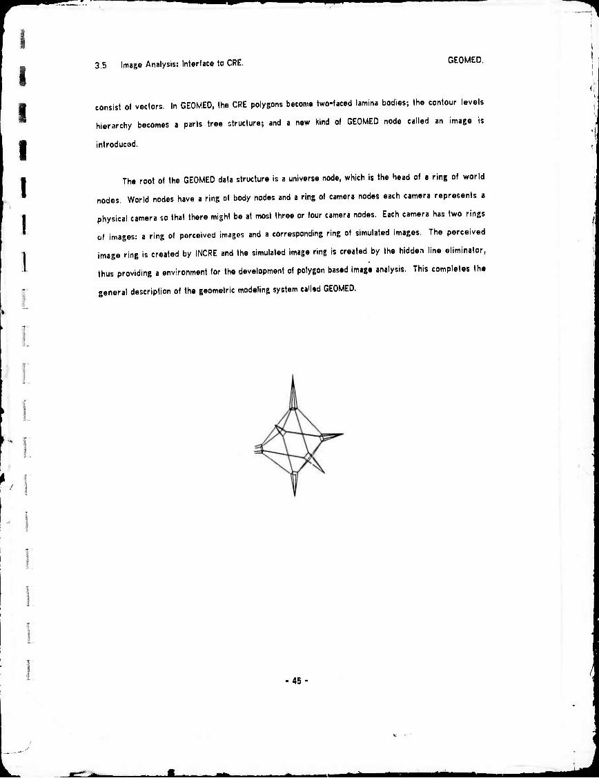
^"
I
I
i
3.5 Image Analysis: Interface to CRE. GEOMED.
consist of vectors. In GEOMED, the CRE polygons become two-faced lamina bodies; the contour levels
hierarchy becomes a parts tree structure; and a new kind of GEOMED node called an image is
introducad.
The root of the GEOMED data structure is a universe node, which is the head of a ring of world
nodes. World nodes have a ring of body nodes and a ring of camera nodes each camera represents a
physical camera so that there might be at most three or four camera nodes. Each camera has two rings
of images: a ring of perceived images and a corresponding ring of simulated images. The perceived
image ring is created by INCRE and the simulated image ring is created by the hidden line eliminator,
thus providing a environment for the development of polygon based image analysis. This completes the
general description of the geometric modeling system ea'led GEOMED.
45
iteHMi

', 0 Introduction to Hidden Line Elimination. OCCULT
SECTION 4.
HIDDEN LINE ELIMINATION FOR COMPUTER VISION.
4.0 Introduction to Hidden Lin« Elimination. 4.1 Initialization and Culling.
4.2 Hide Marking a Coherent Object.
4.3 Edge-Edge and Face-Vertex Comparing. 4.4 Recursive Windowing. 4.5 Photometric Modeling and Video Generation. 4.6 Performance of OCCULT and Related Work.
4.0 Introduction to Hidden Line Elimination.
Hidden line elimination refers to the process of simulating the appearance of opaque three
dimensional objects. The phrase hidden line elimination dates from when the problem only involved
deleting the undesired, that is the hidden lines, from a line drawing (Figure 4.1); today the phrase
persists but connotes the wider problem of synthesizing realistic images using a computer. The
present discussion is about techniques which have been implemented in a particular hidden line
eliminator named OCCULT, from the Latin word oeculiare meaning to hide. OCCULT illustrates novel
solutions to the graphics problems of exploiting object coherence and image coherence, of combining
image space with model space techniques, and of sorting faces, edges and vertices in two dimensions.
OCCULT is further characterized by its intended application to computer vision and robotics. The
distinguishing design requirement of a hidden line eliminator intended for vision is that it must maintain
back pointers from the final 2-D images to the initial 3-D models so that the identity of features can be
recovered. In computer graphics, the results of hidden line elimination are intended for human viewing
46
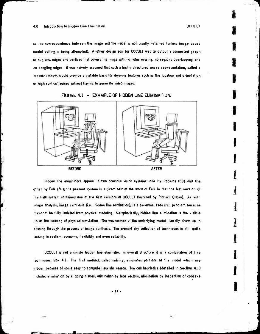
4.0 Introduction to Hidden Line Elimination. OCCULT
so tne correspondence between the image and the model is not usually retained (unless image based
model editing is being attempted). Another design goal for OCCULT was to output a connected graph
ot regions, edges and vertices that covers the image with no holes missing, no regions overlapping and
no dangling edges. It was naively assumed that such a highly structured image representation, called a
momir. imngr, would provide a suitable basis for deriving features such as the location and orientation
of high contrast edges without having to generate video images.
FIGURE 4.1 - EXAMPLE OF HIDDEN LINE ELIMINATION.
BEFORE AFTER
Hidden line eliminators appear in two previous vision systems: one by Robert« (63) and the
other by FalK (70); the present system is a direct heir of the worK of FalK in that the last version of
tn« Falk system contained one of the first versions of OCCULT (installed by Richard Orban). As with
image analysis, image synthesis (i.e. hidden line elimination), is a perennial research problem because
it cjnnot be fully isolated from physical modeling. Metaphorically, hidden line elimination is the visible
tip of the iceberg of physical simulation. The weaknesses of the underlying model literally show up in
passing through the process of image synthesis. The present day collection of techniques is still quite
lacking in realism, economy, flexibility and even reliability.
OCCULT is not a simple hidden line eliminator. In overall structure it is a combination of five
tttdiniques. Box 4.1. The first method, called culling, eliminates portions of the model which are
hidden because of some easy to compute heuristic reason. The cull heuristics (detailed in Section 4.1)
nclnde: elimination by clipping planes, elimination by face vectors, elimination by inspection of concave
47
I i
f I I I I /
^^w
I I
4.1 Initialization and Culling. OCCULT
corners, and elimination by previous occultation. After the culls have been applied, the next three
techniques are arranged in a three level heirarchy which comprises the main part of OCCULT. At the
outermost level there is a WarnocK (68) like recursive windowing method, which calls an edge-edge
comparing method on small enough windows, which in turn calls a coherent object tracing method to
split off and mark the portions of an object that are hidden. The methods are explained in bottom-up
order: hide tracing in Section 4.2, edge-edge comparing in Section 4.3 and recursive windowing in
Section 4.4. The fifth technique is a face-vertex compare method that is occasionally required to solve
a particular class of cases that are missed by the edge-edge compare. The difficult part in building an
OCCULT like hidden line eliminator lies in getting all the unruly beasts in harness together; the
mystery being that no one beast is sufficiently strong to carry the whole burden by itself.
/<
.1
BOX 4.1 THE FIVE HIDDEN LINE ELIMINATION TECHNIQUES OF OCCULT.
1. Initialization Hide Culling.
2. Recursive Windowing.
3. Coherent Object Hide Tracing.
4. Edge-Edge Comparing.
5. Face-Vertex Comparing.
"N
4.1 Initialization and Culling.
A substantial part of sophisticated hidden line elimination lies in careful attention to initial
preparations. As it has now stood for the past two years, OCCULT has two input restrictions imposed
for the sake of execution speed: no conflicting bodies are allowed and no concave faces are allowed.
Conflicting bodies are those that occupy the same space at the same time; concave faces are faces with
interiors containing a pair of points such that the line segment between the points is not contained in
the face. The rational for both these restrictions is based on the optimization technique of getting
computations out of inner loops; conflicting bodies and concave faces can be eliminated by employing
certain polyhedral construction primitives prior to hidden line elimination. The restrictions are not
inherent limitations of any of the techniques in OCCULT, so that a lass restricted but slower
implementation is feasible.
48

4.1 Initialization and Culling. OCCULT
OCCULT is a marking algorithm, the temporary marking bits are listed in Box 4.2. The
combination (POTENT and -VISIBLE) means potentially visible; (-POTENT and VISIBLE) means actually
visible; (-POTENT and -VISIBLE) means hidden; and the combination (POTENT and VISIBLE) is an unused
state that happens to be interpreted as VISIBLE.
"BOX 4.2 STATUS BITS FOR OCCULT MARKINGS.
POTENT Potentially Visible Entity.
VISIBLE Actually Visible Entity. P22 Behind the camera image plane, Positive Zee.
N2Z Before the camera image plane. Negative Zee.
TMPBIT Temporary Split edge of vertex.
POLDEO Edge with only one POTENT face.
JOTBIT Joint over T vertex.
JLTTBIT Joint under T vertex.
The initialization is performed in three steps: (1). vertex marking and vertex perspective
projection; (2). face marking, face Z-clipping, and computation of face coefficients; and (3). edge
marking and computation of edge coefficients. Two cull heuristics are done during the initialization:
clipping and backside faee elimination; and the other two culls are done immediately afterwards:
concave corners cheek and the hide last hidden cheek.
Vertex initialization includes the prospective projection of every vertex in the model and the
marking of every vortex that is in front of the camera as POTENT (potentially visible) if its perspective
projected Z coordinate, ZPP(V), is greater than the simulated image plane distance, FOCAL. Two
further status bits, named PZZ and NZZ, indicate positive ZCC (camera coordinates) or negative ZCC
are inclusive ORod into all the faces and edges of each vertex for the sake of the Z-elipper.
Face initialization consists of Z-clipping: if a faee has only its NZZ bit turned on, then it is
completely behind the camera and is immediately dropped from all futher eondsideration (i.e. culled
out); if the face has both its PZZ and its NZZ turn on then it is Z-clipped by using the camera's image
plane as a cutting plane. Next for faces in view of the camera, the 3-D perspective projected face
coefficients are computed (equations given below) and the faces with their backsides towards the
camera are culled out (Figure 4.2); faces surviving to this point are marked as POTENT and are placed
into a list of faces of the first window of the recursive window sort.
49
i
1 /
^ria


«w
4 2 Hido Marking a Coherent Object OCCULT
ddges that are easily discovered to be hidden (i.e the end of the edge that is connected to the corner
is hidden by a face of that corner) The second cull is applicable when hidden line elimination is being
done on a sequence of images which are not changing very much from one picture to the next. By
saving a pointer to the nrrrfum that covered each hidden vertex in the immediately preceding hidden
line olimmation, the previous overface can be quickly checked to see if it still covers the vertex In the
case of arm animation (example «2, Section 3.0) this form of exploiting frnmr-rolirmtcr realized a
twenty-five percent savings in computation time (under timesharing, but with no other user programs).
FIGURE 4.3 - FRONT FACES AND FOLDS OF A CONCAVE CORNER.
inspite of the complexity explained so far, still further measures could be taken to make 'he
hidden line eliminator even faster, For example more 3-D clipping or spatial recusive ceil sorting would
allow the earlier elimination of objects that are out of sight.
4.2 Hide Marking a Coherent Object.
OCCULT marks the faces, edges and vertices of a polyhedral scene as being either visible or
hidden with respect to a simulated camera Edges that were at first partially visible are split into
pieces so that each piece is either fully visible or fully hidden. All splits are undone and all OCCULT
bits are cleared by a fixup routine named UNCULT. In a modeling environment that provides coherent
polyhedea that can be easily traveled and modified, the simple techniqu« of hide marking the neighbors
of entities already hidden can be used to do almost all of the actual hiding, one« a starting place has
been found.
In OCCULT, the two innermost routines, EHIDE and VHIDE, perform this kind of marking and
splitting The routine VHIDE takes two arguments: the vertex, V, which is to be marked as hidden and
the face, F, that is known to hide V; the rou'ine then simply calls EHIDE for each potentially visible
51
!
I
I

^^ mmm
4.3 Edge-Edge and Face-Vertex Comparing. OCCULT
I 1
I
edge of V's perimeter. EHIDE in turn takes three arguments: an overface, F, an edse, E. and one
vertex, V, of that edge which is known to be hidden by F. EHIDE then checks to see wnether or not E
leaves its overface, F, there are three basic cases: (i) E does no! leave F, so it is marked as hidden
and VHIDE is applied to the verlax 0THER(E,V); (ii) E does leave overface F by crossing under a
-FOLDED edge which provides a new overface for EHIDE to check; or (iii) E leaven F by crossing under
a folded edge, so EHIDE splits the original edge, E, and the folded edge to form a T-jomt (exolained
below) marking the hidden portion of E as hidden and leaving the remaining portion of E potentially
visible.
A T-joint occurs in the image, when a folded edge hides a second edf»e that L further away
from the camera. When OCCULT discovers a T-joint, both edges are ESPLIT and two n«w vflrtifer ?r6
created the further one is called the JUT, Joint-Under-T, vertex the nearer one is called the JOT,
Joint-Over-T, vertex. Juts and Jots point at each other using a temporary link field named TJOINT.
FIGURE 44 - T-JOINT DIAGRAM.
(The dufinm it i view from sliRhlly to the left and below the cimen from which JOT »nd JUT auoMr eomodert /
l
FOLD
.EDGE
JUT
JOT
There are several techniques for finding hidden starting places, the major techniques involve
doing an edge-edge or a face-vertex compare using all the potentially visible (aces, edges and
vertices; the minor techniques include the concave corner cull and the hidden on last hide cull
4.3 Edge-Edge and Face-Vertex Comparing.
In OCCULT, two particular compares stand out as most basic, the edge-odge comoaro and the
face-vertex compare which are implemented in procedures named COMPEE and COMPFV, respectively.
52
- ii

A 3 Edge-Edga and Face-Vertex Comparing. OCCULT
Tho odge-odge compare routine, COMPEE, determines whether or not two edges intersect in the 2-D
image coordinates, XPP and YPP. The basic edge-edge intersection test requires passing two
opposition conditions: the ends of one edge must be in the opposite halfplane with respect to the line
containing the other edge and vice versa. Halfplane opposition is checked by two evaluating the normal
equation of the line using the edgo coefficients AA, BB, CO and the vertex coordinates XPP and YPP.
Consequently, it can be assumed tliat the two edges cross if the following expressions both return
negative values:
FLflCl - lfiB(El)*XPP(PVT(E2)) ♦ BB(E1)«YPP(PVT(E2)) ♦CC(El)) XOR tRfl(El)«XPP(NVT(E2)) ♦ BBIE1)«YPP(NVT(E2)) ♦ CC(E1));
PLRC: ► (fiR(E2)*XPP(PVT(El)) ♦ BB (E2)4VPP (PVT (El)) ♦CC(E2)) XOR (RP(E2)«XPP(NVT(E1)) ♦ BB(E2)«YPP(NVT(E1)) ♦CCtE2))|
The infix operator XOR (exclusive OR) is for toggling the sign bits in the same fashion as a
multiplication would in more conventional ALGOL. When the crossing condition is tru«, the locus of
intersection can be computed by solving two equations in two unknowns:
TMP XPP(V) VPPW)
(flfl(El) .BBIE2I - nR(E:);PB(Ei))i ICC (ED ;BBIE2I - CC(E21 :E>B(E1))/TMP| (flfl(El):CC(E2) - RR(E2l~CC(El))/TnPi
An alternate edge-edgo compare method would be to solve the two equations in two unknowns
first and then to see whether the intersection locus is interior to the line segments of both edges.
Since, disjoint pairs of edges occur much more frequently than intersecting edges, the alternate method
requires more floating arithmetic on the average than the first method which can discover about half of
the disjoint cases by computing FLAG1. Furthermore the alternate method does not lend itself to
distinguishing the almost touching cases which must be nudged to be disjoint. The OCCULT design
depends on coercing edges to intersect at one unique point or not at all, the steps listed in Box 4.4
handle the special cases requiste to such a crossing discipline. The nudge is done in image coordinates,
so the accuracy of world coordinates is maintained.
y'BOX 4.4 Edge-Edge Compare Steps.
i. Test for Identity: same edge twice.
li. Test for Topological connection: Edges with vertex or T-joint in common,
hi. Test for span Overlap in XPP and YPP: To prevent nasty collinear cases.
iv. Compare for crossing: Opposition Tests and Crossing Solver,
v. Nudge (Move off line, towards right and down).
"N
I I I I I
I I I
53-

i^^w
4.3 Edge-Edge and Face-Vertex Comparing. OCCULT
I I i I I I I
I
I I I I
The lace-vertex compare routine, COMPFV has two parts: /.-dcfiih rompnrc for vertex under
the plane of the lace, and 2-1) within rompnrc for vertex enclosure by the face perimeter The first
compare is done by evaluating the Z-depth of the vertex with respect to the plane ot the face. The
second comparo tests whether the vertex falls outside of the face with respect to any of the edges of
the face perimeter, since faces are convex and since polyhedra are oriented the o.:erly directed
edges coefficient are available. The Z-depth test is performed first because it is quickt
Two very simple but important kinds of hidden line eliminators (that almost work) are based on
combining edge-edge comparing or face-vertex comparing with coherent object hiding, In the
edge-edge compare method all the edges (or even merely all the folded edges) of the image are
compared with each other, N)t<{N-l)/2 compares, for crossings; when a crossing is found a T-joint is
made and the hidden portion of the under edge is given to an EHIDE routine. In the face-vertex
compare method all the vertices are compared with all the faces, (face count)*(vertex count) compares,
for enclosure and covering; when a vertex is found hidden under and within a face it is given to a
VHIDE routine. Together the EE-compare method and the FV-compare method form one slow but sure
hidden line olimination algorithm; alono the EE-method fails to detect hidden objects with edges that
don't intersect any edges of the occluding object as in the left panel of Figure 4 5 which shows two
bricks of the same size but one behind the other. Likewise the FV-method fails to detect hidden
objects in scenes where no vertex of the object is surround or covered by a face, right panel of
Figure 4.5.
In OCCULT, the edge-edge compare is done after recursive windowing has isolated a reasonably
small number of edges (twelve). A face-vertex compare is done only if any potentially visible vertices
remain after all the other techniques have finished; in particular face-vertex comparing is only done
when the case illustrated in the left panel of Figure 4.5 actually occurs and the set of faces that are
used are only the faces that intersect the recursive window that contains the vertex.
-54-
^k

^•w
4.4 Recursive Windowing. OCCULT
FIGURE 4.5 - EE AND FV UNDETECTED HIDDEN OBJECT CASES.
I I I
EDGE-EDGE FAILURE CASE, FACE-VERTEX FAILURE CASE.
4.4 Recursive Windowing.
Recursive Windowing is a two dimensional spatial sorting technique for partitioning the faces,
edges and vertices associated with a rectangular region called a window into two subwindows. The
technique is applied recursively until a desired condition is achieved. The usual termination condition is
that the population of entiles in the window becomes sufficiently low or that the window becomes
extremely small. The idea is implement in a routine called ESORT which resembles the hidden line
eliminators of (WarnocK 68) and (Sutherland 69). However ESORT is unique in that it maintains a data
structure which allows edges to be split during the sort. The potentially nasty fixups are accomplished
using a aata structure that maintains a coherent image of both windows and edges. Metaphorically, the
data structure is a cloth with a warp of windows and a woof of edges, where each warp thread is
bound to a woof fiber by a bead.
Window Simriurc. The sort window itself is a twelve word node which contains data fields
ndmed XLO, XHI, YLO and YHI which specify the boundary of the window and data fields named
PENCNT, SURCNT, EDGCNT and VCNT which specify the number of faces that penetrate the window,
the number of faces that surround the window, the number of edges that pass through the window and
the number of vertices that fall within the window, respectively. The window contains link fields to
55
^*m

mm
I I I
4.4 Recursive Windowing. OCCULT
hold pointers to the head cl the pon-face list (penetrating faces), the sur-face list (surrounding faces),
the vertex list, the head and tail the edge list and a pointer to its antecedent window.
lirnd Siniriuro A bead is a two word node that contains four pointers and which represents
one instance of an edge passing through a window. Each edge has a list of beads representing an
ordered list of the windows through which it passes; and each window has a list of beads representing
a list of the edges it contains. The link fields named WND and EDG of a bead, point to the particular
window and the particular edge to which the bead belongs. The link fields named WNBL and EDBL of a
bead contain the necessary links for the window's bead list and for the edge's bead list.
BOX 4 5 RECURSIVE WINDOWING ROUTINES.
1. MKSWN Make Sort Window.
2. PSHSWN Push Sort Window.
3. PENSUR Update penetrator and surrounder lists.
4. POPSWN Pop Sort Window.
5. BLED Bead List Edit.
The actual sort is composed of five routines (Box 4.5) which perform all the necessary creations
and alterations to the window/edge/bead data structure. Initialization is done by the make sort window
routine, MKSWN, which places all the potentially visible faces, edges and vertices into the first sort
window along with the population counts and the extreme location of vertices in the positive and
negative, XPP and YPP directions.
If the population counts of the window are too large, the pushdown sort windowing routine,
PSHSWN, creates a new window node, places the node into the sort-window pushdown list, halves the
original window's rectangle (spliting the longer sides) leaving the left (or upper) half of the rectangle
in the old window node and allocating the right (or lower) half to the new window node. Next the
vertex list is partitioned, each vertex falls into only one or the other window. Next the original
window's bead list of penetrating edge is scanned, each edge must fall into one or the other or both
windows. If an edge falls into both windows then a new bead is made and is placed in order into the
bead list of the edge so that the beads of every edge indicate window penetrations in order from
upper-left-most to lower-right-most. Finally PSHSWN applies PENSUR to each of the two windows.
56

4 4 Recursive Windowing. OCCULT
The penettator and surrounder (ace routine, PENSUR, scans the new bead lists o< penetrating edges o<
the two suowindows and marks the faces oi those edges as penetrators and places them on the pen-list
of the new window; next the routine scans the old penetrator list of the parent window and tests (and
clears) the markings. Unmarked faces must be either surrounders or outsiders; the surrounders are
placed in the sur-list of the new window.
If the populations of the window are sufficiently low the hidden line eliminator (or the body
interboctor, Chapter 5) processes the window (does the edge-edge compares) and ca Is the pop sort
window routine, POPSWN POPSWN zeroes the window field, WND, of beads of the window as an
indication that the window is dead and so are its beads; dead beacic an returned to free storage by
the BLED routine explained below. Next the POPSWN scans the vertices or the window and places th«
pen-list and sur-list pointers of the window into temporary fields of each vertex; this trick preserves
the results ot the recursive window sort for the sake of possible face-vertex comparing. Finally the
window node is popped off the pushdown window list and returned to free storage.
During both hidden line elimination and body intersection, edges are split in order to isolate the
portion that is hidden or in order to create face piercing points. When an edge is split its bead list of
windows is also split by means of the bead list edit routine, BLED. Since beads of an edge are ordered
upper-left to lower-right; the BLED routine scans the beads for the window into which the newly
;redt«d spht vertex falls within; the vertex is then placed on that window's vertex list and a new bead
is created (since both the old and the new edges must have beads in the window that contains the split)
and the old bead list is split. Dead beads that are found while scanning the bead list ar« returned to
free storage
Although the link manipulations are complicated to recite, the essential point is that both
windows and edges can be split without losing their topologieal connectedness, which gives one a tool
(or reducing an N-squared spatial computation into an N-log-N computation. The present
implementation is coded in PDP-10 machine code, an ALGOL publication version will appear in a
forthcoming technical report which is beyond the scop« of this paper.
57
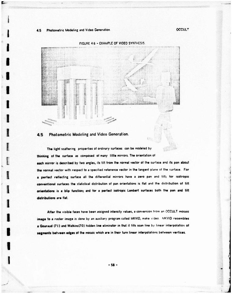


I I I
..
!
1 I
5.0 Introduction to Polyhedron Inlorsection. POLYHEDRON INTERSECTION.
SECTION 5.
POLYHEDRON INTERSECTION.
5.0 Introduction to Polyhedron Intersection.
5.1 Intersection Geometry.
5.2 Intersoction Topology.
5.3 Special Cases of Intersection.
5.4 Face Convexity Coercion.
5.5 Body Cutting. 5.6 Performance and Related Work.
5.0 Introduction to Polyhedron Intersection.
The intersection, union, and set differences of two solid polyhedra can be computed by
combining a body intersection procedure called BIN with the EVERT primitive, as Figur» 5.1 illustrates.
The body intersection procedure is important for three reasons: first, it is a general and conceptually
elegant construction operator; second, it can be used for spatial modeling <" collision detection and
trajectory planning for manipulators and vehicles; and third, it can be used to localize an object in 3-D
space from a sequence of silhouotto viows. The intersection algorithm consists of two parts: first,
there is a geometric part in which all the faces and edges are compared with each other for potential
face/edge intersections called piercing points; and second, there is a topoiogical part in which the
results are "copied off" of the given polyhedra; the results may consist e' zero, one or many
polyhedra. In the following, the term "operands" refers to the sett of polynedra given to BIN ••
arguments and the term "result" refers to the set (possibly empty) of polyhedra produced by BIN.
-60
^^h


1
I I I
I I
I 1
I 1 I
5.1 Intersection Geometry. POLVHEDTON INTERSECTION.
5.1 Intersection Geometry.
Conceptually, the geometric part of the polyhedron intersection algorithm, BIN, consists of
* comparing each face of one operand with every edge of the other operand and vice versa. In practice
the potentially N-squared compares are avoided by using the same recursive window partition sort that
was used in the hidden line eliminator, OCCULT, Section '..3. Ignoring the recursive windowing for a
moment, the innermost face-edge compare of BIN consists of four steps: opposition, intersection,
enclosure and fission.
FIGURE 5.2 - FACE PIERCING GEOMETRY.
Piercing Point Within F. Piercing Point outside F.
Oniuniiion 7V.W. Given a face F and an odge E, first, the endpoints of the edge are checked to
see whether they are in opposite halfspaces with respect to the plane of the face In terms of vector
geometry, the dot product of the lace vector and each vertex vector is taken and the signs compared;
different signs indicate that the vertices are in different halfspaces. The opposition test requires six
multiplications, httpniunhn l.nrns. The locus of the point where the edge pierces the plane of the
face is computed (four multiplications). Ijjirhmrv Test. Next the edge is tested to see if it actually
passes thru the interior of the face. In BIN, this test exploits the face convexity restriction The test
consists of crossing neighboring pairs of vectors radiating from the face-plane piercmg-pomt to each
vertex of the given face and testing for a sign change, Figure 5.2. Since only one component of the
cross product needs to be evaluated, the test requires only two multiplications per edge of the face
whoes plane is pierced. KHso Fimon. If the edge pierces the face, then the edge is split (using the
ESPLIT and BLED routines) forming a new vsrtex, called a face piercing vertex A temporary link of
the vertex node (field CW, left half of word 7) is set to point at the face that was pierced and the PED
link of the new vertex is set to point at the one of its two edges that is external to the surface.
-62
- *
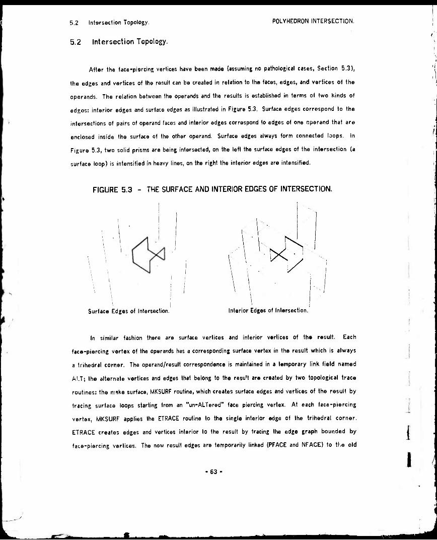
5.2 IntorsGction Topology POLYHEDRON INTERSECTION.
5.2 Intersection Topology.
After the face-piercing vertices have been made (assuming no pathological cases, Section 5.3),
the edges and vertices of the result can be created in relation to the faces, edges, and vertices of the
operands. The relation between the operands and the results is established in terms of two kinds of
edges: interior edges and surface edges as illustrated in Figure 5.3. Surface edges correspond to the
intersections of pairs of operand faces and interior edges correspond to edges of one operand that are
enclosed inside the surface of the other operand. Surface edges always form connected loops. In
Figure 5.3, two solid prisms are being intersected, on the loft the surface edges of the intersection (a
surface loop) is intensified in heavy lines, on the right the interior edges are intensified.
FIGURE 5.3 - THE SURFACE AND INTERIOR EDGES OF INTERSECTION.
i i I
Surface Edges of Intersection.
^
Interior Edges of Intersection.
In similar fashion there are surface vertices and interior vertices of the result. Each
face-piercing vertex of the operands has a corresponding surface vertex in the result which is always
a trihedral corner. The operand/result correspondence is maintained in a temporary link field named
ALT; the alternate vertices and edges that belong to the result are created by two topological trace
routines: the nuke surface, MKSURF routine, which creates surface edges and vertices of the result by
tracing surface loops starting from an "un-ALTered" face piercing vertex. At each face-piercing
vertex, MKSURF applies the ETRACE routine to the single interior edge of the trihedral corner.
ETRACE creates edges and vertices interior to the result by tracing the edge graph bounded by
face-piercing vertices. The now result edges are temporarily linked (PFACE and NFACE) to the old
63
i I i
*m

5.2 Intersection Topology POLYHEDRON INTERSECTION.
I I I I
operand faces. The MKSURF and ETRACE routines are followed by three step', that fix up the -.urface
wings, interior wings and face nodes so that a complete winged edge polyhedral result is legally
formed.
The interior trace routine is iriv^l - all the links are readily accessed using the ECCW and
OTHER primitives on the operand poly'iedra. The surface trace routine is made easy by implementing a
procedure, NEXTPV, to retrieve the next face-piercing vertex about a surface loop The NEXTPV
procedure, given below, is based on the obseravtion that the intersection of two convex faces is one
line segment and either one face is pierced twice by two different edges of the other face; or each
face is pierced once by one edge ci the other face, Figure 5.4.
I FIGURE 5.4 - FETCH NEXT FACE-PIERCING VERTEX.
Edge of Fl pierces F2 at V2. Edge of F2 pierces FI at V2
;
I
COnnENT RETURN THE NEXT FfiCE PIERCING VEXT Of R SURfflCE LOOP;
INTEGER PROCEDURE NEXTPV (INTEGER F2,V1I;
BEGIN "NEXTPV"
INTEGER F1,V2| Fi .. CUCVIM COMflENT FACE PIERCED BY VI;
COMtlENT DOES PN EDGE OF Fl PIERCE F2 AT THE OTHER PIERCE-VERTEX V2;
E ► EO ► PE0IF1);
DO IF F2 = CU(V:yVCCU(E,Fl)) THEN RETURN(V2) UNTIL EO » (E-ECCU (E ,f 1) I ;
COnriENT DOES PN EDGE OF F2 PIERCE Fl PT THE OTHER PIERCE-VERTEX V2;
E - EO - PED(F2);
DO IF Fl , CU(V2-VCCU(E,F1)) i- V2.V1 THEN RETURNS) UNTIL EO . (^ECCUIE.FZ) >;
COHflENT FPTPL CONSISTENCY ERROR - SOUETHINC WRONG IN FPCE/EDGE COtlPflRE PS3S;
PETURN(O);
END "NEXTPV";
Fix up stop-l places vertex and wing pointers in all the interior edgns An interior edge is
distinguished by its non-zero ALT link, The new vertices are provided with a first odge, PED(VNEW),
if it be lacking. Fix up step-2 wings together the surface vertex tridedral corners Since by good luck
-64-
^Ü ^rik MH

T 5 3 Special Cases of Internoclion POLYHEDRON INTERSECTION.
.ill surface vertices are necessarily trihedral, the edges can be passed to the WING primitive for
oriented linking, in any order The two surface wings of a surface vertex were stored in the NED and
FED links by MKSURF; the inward wing can be retrieve as the FED(ALT{U)). Surface vertices are
distinguished by their ALT vertex being marked as a piercing vertex. Fix up step-3 replaces the alien
faces of the result with nativa faces. This is done by scanning the edge ring of the body, testing the
two faces of each edge to see if they belong to the result body, and if a face doesn't belong it is
replaced by a new one. Face replacement, as ususal, requires clocking around a face perimeter and
changing the appropriate lace link in each edge. A final marking trace assigns one body node to each
separate connected graph of faces, edges and vertices.
I I
FIGURE 5.5 - EXAMPLE OF A FACE HOLE FIXUP.
5.3 Special Cases of Intersection.
In order of difficulty from easy to hard, the four special cases that must be han'iled are
non-intersection, extremely short edges, face holes and coincident entities. Non-h\irrsrriinn. When
the face-edge compare (by recursive window space sort) returns no piercing points, it implies that the
surfaces of the given polyhedra do not intersect and that a further test is needed to determine
whether the operands are disjoint (and so the intersection be empty) or whether one operand contains
the other, rnm llnlrs. Because EVERTod solids are allowed, one polyhedron can cut a hole in a face
of the other without intersecting any of the edges of that face, which would fool the copy-trace. So as
a preliminary step to BIN, all the surface loops are traced and checked to make certain they cross
more than one face. If a one face surface-loop is found, the face is pyramided to a vertex interior to
the surface-loop. A face hole fix up is illustrated in Figure 5.5, the middle panel of the figure shows
65 - I
MM mam—m

5.5 Body Cutting, POLYHEDRON INTERSECTION.
I
I I I
that two faces of the cubic prism wore pyramided, the right panel of the figure shows the result after
face-convexity coercion. .S'/»ir( I'.'l, r<. An application of BIN can create edges with almost zero length,
which require an extra pass to lind and delete. Omridnu EniUiw. An occasional edge that lie-,
exactly in the plane of a face can be nudged off the plane a little resulting in extremely short edges
which are later removed. Although it is meaningful to try to intersect polyhedra which have many
faces, edges and vertices that are exactly coincident, the present implementation loses track of interior
and exterior when too many nearly zero length edges are made.
5.4 Face Convexity Coercion.
Since, both the body intersecter, BIN, and the hidden line eliminator, OCCULT, are restricted to
convex faced polyhdera; it is essential to have a routine that detects and subdivides the concave faces
of a given polyhedron. The make convex routine, MKCNVX, reduces the concave faces of a body into
reasonably small number of convex faces The method consists of two steps: first, the face is broken
down into triangles and second, the longest unnecessary newly made edges are removed. The
reduction to triangles step is recursive: the pointiest extrema vertex of a face, VO, is lopped off, if no
other vertices of the face are on the same side of the line segment between VO's immediate
neighboring vertices: OTHER(ECCW(V0,F),V0) and 0THER(ECW(V0,F),V0). Otherwise the face is split,
MKFE, using the vertex closest to VO that violates VO's potential lop line. An extrema vertex is one
that touchs the smallest circumscribed rectangle whose sides are parellel to 'he coordinate axes; the
pointiest vertex is the one with fhe largest cosine.
FIGURE 5.6 - EXAMPLES OF FACE CONVEXITY COERCION.
5.5 Body Cutting.
Body cutting is the operation of dividing an arbitrary polyhedron into sets of parts above and
66 -
JHh rtuta mm
5 6 PeHorrtidnce and Related Work POLYHEDRON INTERSECTION.
below a given cutting plane, as has already been illustrated in Figure 3.8. Although body cutting might
be done by subtracting a very large thin rectangular prism, the process is sufficiently important to
merit a separate implementation which nevertheless resembles the subtraction. First, all the edges of
the given body are compared with the given cutting plane and piercing vertices are formed in pairs
(one vertox for each side of the cut). Between the cutting-plane vertex-pairs are zero length edges
which are placed into a special temporary list. Next, pairs of cutting-plane vertices (belonging to the
same face and dest ^ed to be in the same half-space) are MKFEed together splitting the faces with
cutting-plane edge pairs (one edge for each side of the cut). Between the cutting-plane edge-pairs
are zero area faces. Finally all the zero length cutting plane edges are KLFEed if their PFACE and
NrACE are different or UNGLUEed if thoir PFACE and NFACE are the same. In this circumstance an
er.ge having the same NFACE and PFACE is a wasp edge. The simplicity of the body cutting
implementation is do to the power of the UNGLUE Euler primitive.
5.6 Performance and Related Work.
Curious to relate, I have found no example in the literature of a general polyhedron intersection
method. Maruyama's (72) method is a collision detector rather than a intersector, because he does not
attempt to generate the polyhodra of intersection; however, his algorithm does resemble the geometric
first phase of BIN and might have been extended for generating new solids. The intersection methods
of Braid (73) are restricted to particular combinations of six volume elements which comprise a useful
subset of cases for mechanical drawing.
The version of BIN is implemented on a PDP-10 (with 2 microsecond core memory) can
construct the intersection of simple objects such as a pair of cubes in less than a quarter of a second;
the intersection of a couple of twenty sided cylinders in about two seconds; the intersection of two
horse silhouette cones takes (chapter 9) about fifteen seconds; and the intersection of two silhouette
cone intersections can take up to a minute.
67
.a^i ^Mta

6.1 A Geometric Feedback Vision System. VISION THEORY.
SECTION 6.
COMPUTER VISION THEORY.
6.0 Introduction to Computer Vision Theory. 6.1 A Geometric Feedback Vision System. 6.2 Vision Tasks. 6.3 Vision System Design Arguments. 6.4 Mobile Robot Vision. 6.5 Summary and Related Vision Work.
6.0 Introduction to Computer Vision Theory.
Computer vision concerns programming a computer to do a task that demands the use of an
image forming light sensor such as a television camera. The theory I intend to elaborate is that
general 3-D vision is a continuous process of keeping an internal visual simulator in sync with
perceived images of the external reality, so that vision tasks can be done more by reference to the
simulator's model and less by reference to the original images. The word theory, as used here, means
simply a set of statements presenting a systematic view of a subject; specifically, I wish to exclude the
connotation that the theory is a natural theory of vision. Perhaps there can be such a thing as an
artificial theory which extends from the philosophy thru the design of an artifact.
6.1 A Geometric Feedback Vision System.
Vision systems mediate between images and world models; these two extremes of a vision
system are called, in the jargon, the bottom and the top respectively. In what follows, the word
image will be used to refer to the notion of a 2-D data structure representing a picture; a picture
-68
JL_ . Mi ~ —-^
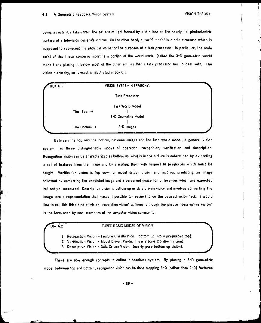
6.1 A Geometric Feedback Vision System. VISION THEORY.
being a rectangle taken from the pattern of light formed by a thin lens on the nearly flat photoelectric
surface of a television camera's vidicon. On the other hand, a world modrl is a data structure which is
supposed to represent the physical world for the purposes of a task processor. In particular, the main
point of this thesis concerns isolating a portion of the world model (called the 3-D geometric world
model) and placing it below most of the other entities that a task processor has to deal with. The
vision hierarchy, so formed, is illustrated in box 6.1.
/'BO BOX 6.1
The Top
The Bottom
VISION SYSTEM HIERARCHY.
Task Processor
I Task World Model
I 3-D Geometric Model
I 2-D Images
Between the top and the bottom, between images and the task world model, a general vision
system has three distinguishable modes of operation: recognition, verification and description.
Recognition vision can be characterized as bottom up, what is in the picture is determined by extracting
a set of features from the image and by classifing them with respect to prejudices which must be
taught. Verification vision is top down or model driven vision, and involves predicting an image
followed by comparing the predicted image and a perceived image for differences which are expected
but not yet measured. Descriptive vision is bottom up or data driven vision and involves converting the
image into a representation that makes it possible (or easier) to do the desired vision task. I would
like to call this third kind of vision "revelation vision" at times, although the phrase "descriptive vision"
is the term used by most members of the computer vision community.
Box 6.2 THREE BASIC MODES OF VISION.
1. Recognition Vision - Feature Classification, (bottom up into a prejudiced top).
2. Verification Vision - Model Driven Vision, (nearly pure top down vision).
3. Descriptive Vision - Data Driven Vision, (nearly pure bottom up vision).
There are now enough concepts to outline a feedback system. By placing a 3-D geometric
model between top and bottom; recognition vision can be dote mapping 3-D (rather than 2-D) fertures
69
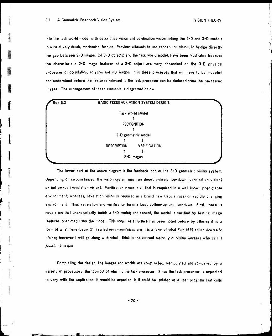
6.1 A Geomelric Feedback Vision System. VISION THEORY.
I
info the task world model with descriptive vision and verification vision linking the 2-D and 3-D models
in a relatively dumb, mechanical fashion. Previous attempts to use recognition vision, to bridge directly
the gap between 2-D images (of 3-D objects) and the task world model, have been frustrated because
the characteristic 2-D image features of a 3-0 object are very dependent on the 3-D physical
processes of occultation, rotation and illumination. It is these processes that will have to be modeled
and understood before the features relevant to the task processor can be deduced from the peiceived
images. The arrangement of these elements is diagramed below.
Box 6.3 BASIC FEEDBACK VISION SYSTEM DESIGN.
Task World Model
T
RECOGNITION
T
3-D geometric model
t i
DESCRIPTION VERIFICATION
T i 2-D images
The lower part of the above diagram is the feedback loop of the 3-D geometric vision system.
Depending on circumstances, the vision system may run almost entirely top-down (verification vision)
or bottom-up (revelation vision). Verification vision is all that is required in a well known predictable
environment; whereas, revelation vision is required in a brand new (tabula rasa) or rapidly changing
environment. Thus revelation and verification form a loop, bottom-up and top-down. First, there is
revelation that unprejudically builds a 3-D model; and second, the model is verified by testing image
features predicted from the model. This loop like structure has been noted before by others; it is a
form of what Tenenbaum (71) called accommodmion and it is a form of what Falk (69) called heuristic
vision; however I will go along with what I think is the current majority of vision workers who call it
fecdhnck vision.
Completing the design, the images and worlds are constructed, manipulated and compared by a
variety of processors, the topmost of which is the task processor. Since the task processor is expected
to vary with the application, it would be expedient if it could be isolated as a user program tiat calls
70

6.2 Vision Tasks. VISION THEORY.
on utility routines of an appropriate vision sub-system. Immediately below the task processor are the
3-D recognition routines and the 3-D modeling routines. The modeling routines underlie most
everything because they are used to create, alter and access the models.
Box 6 4 PROCESSORS OF A 3-D VISION SYSTEM. ■^
0. The task processor.
1. 3-D recognition.
2. 3-D modeling routines.
3. Reality simulator.
4. Image analyser.
5. Image synthesizer.
6. Locus solvers.
7. Comparators: 2D and 3D.
The remaining processors include the reality simulator which does mechanics for modeling
motion, collision and gravity. Also there are image analyzers, which do image enhancement and
conversions such as converting video rasters into line drawings. There is an image synthesizer, which
does hidden line and surface elimination, for verification by comparing synthetic images from the model
with perceived images of reality. There are three kinds of locus solvers that compute numerical
descriptions for cameras, light sources and physical objects. Finally, there is of course a large number
of (at least ten) different compare processors for confirming or denying correspondences among
entities in each of the different kinds of images and 3-D models.
6.2 Vision Tasks.
The 3-D vision research problem being discussed is that of finding out how to write programs
that can see in the real world. Related vision problems include: modeling human perception, solving
visual puzzles (non-real world), and developing advanced automation techniques (ad hoc vision). In
order to approach the problem, specific programming tasks are proposed and solutions are sought,
however a programming task is different than a reseach problem because many vision tasks can be
done without vision. The vision solution to be found should be able to deal with real images, should
include the continuity of the visual process in time and space, and should be more general purpose and
less ad hoc. These three requirements (reality, continuity, and generality) will be developed by
surveying six examples of computer vision tasks.
71
WS1 a. ^^

i I I I I
6.2 Vision Tasks. VISION THEORY.
1
BOX 6.5 SIX EXAMPLES OF COMPUTER VISION TASKS.
Cnrl Rrlnlrd Tnskx. 1. The Chau<feur Task.
2. The Explorer Task.
3. The Soldier Task.
Table Top Rrlnlrd Tnskx, 4. Turntable Task.
5. The Blocks Task.
6. Machine Assembly Tasks.
First, there is the robot chauffeur task. In 1969, John McCarthy asked me to consider the vision
requirements of a computer controlled car such as he depicted in an unpublished essay. The idea is
that a user of such an automatic car would request a destination; the robot would select a route from
an internany stored road map; and it would then proceed to its destination using visual data. Tho
problem involves representing the road map in the computer and establishing the correspondence
between the map and the appearance of the road as the automatic chauffeur drives the vehicle along
the selected route. Lacking a computer controlled car, the problem was abstracted to that of tracing a
route along the driveways and parking lots that surround the Stanford A.I. Laboratory using a
television camera and transmitter mounted on a radio controlled electric cart. The robot chauffeur task
could be solved by non-visual means such as by railroad like guidance or by inertial guidance; to
preserve the vision aspect of the problem, no particular artifacts should be required along a route
(landmarks must be found, not placed); and the extent of inertial dead reckoning should be noted.
I I I I I
Second, there is the task of a robot explorer. In (McCarthy 1964) there is a description of a
robot for exploring Mars. The robot explorer was required to run for long periods of time without
human intervention because the signal transmission time to Mars is as great as twenty minutes and
because the 23.5 hour Martian day would place the vehicle out of Earth sight for twelve hours at a
time. (This latter difficulty could be avoided at the expense of having a set of communication relay
satellitfis in orbit around Mars.) The task of the explorer would be to drive around mapping the
surface, looking for interesting features, and doing various experiments. To be prudent, a Mars
explorer should be able to navigate without vision; this can be done by driving slowly and by using a
tactile collision and crevasse detector. I the television system fails, the core samples and so on can
stül be collected at different Martian sites without unusual risk to the vehicle due to visual blindness.
72
■Mi

6.2 Vision Tasks. VISION THEORY.
The third vision task is that of the robot soldier, tank, sentry, pilot or policeman. The problem
has several forms which are quite similar to the chauffeur and the explorer with the additional goal of
doing something to coerce an opponent. Although this vision task has not yet been explicitly attempted
at Stanford, to the best of my knowledge, the reader should be warned that a thorough solution to any
of the other tasks almost assures the Orwellian technology to solve this one.
Fourth, the turntable task is to construct a 3-D model from a sequence of 2-D television images
taken of an object rotated on a turntable. The turntable task was selected as a simplification of the
explorer task and is an example of a nearly pure descriptive vision task.
Fifth, the classic blocks vision task consists oi two parts: first convert a video image into a line
drawing; second, make a selection from a set of predefined prototype models of blocks that accounts
for the line drawing. In my opinion, this vision task emphasizes three pitfalls: single image vision, line
drawings and blocks. The greatest pitfall, in the usual blocks vision task, is the presumption that a
single image is to be solved; thus diverting attention away from the two most important depth
perception mechanisms which are motion parallax and stereo parallax. The second pitfall is that the
usual notion of a perspective line drawing is not a natural intermediate state; but is rather a very
sophisticated and platonic geometric idea. The perfect line drawing lacks photomelnc information; even
a line drawing with perfect shadow lines included will not resemble anything that ran readily be gotten
by processing real television pictures. Curiously, the lack of success in deriving line drawings from
real television images of real blocks has not dampened interest in solving the second part of the
problem. The perfect line drawing puzzle, was first worked on by Guzman (68) and extended to
perfect shadows by Waltz (72); nevertheless, enough remains so that the puzzle will persis» on its own
merits, without being closely relevant to real world computer vision. Even assuming that imperfect line
drawings are given, the blocks themselves, have lead such researchers as Falk (69) ?nd Grape (73) to
concentrate on vertex/edge classification schemes which have not been extended beyond the blocks
domain. The blocks task could be rehabilitated by concentrating on photometric modeling and the use
multiple images for depth perception.
4; I {
(
73 /

mmam
6.3 Vision System Design Arguments VISION THEORY
Sixth, the Stanford Artificial Intelligence Laboratory has recontly (1974) begun work on a
National Science Foundation Grant supporting research in automatic machine assembly. In particular,
effort will be directed to developing techniques that can be demonstrated by automatically assembling a
chain saw gasoline engine. Two vision questions in such a machine assembly task are, where is the
part and where is the hole; these questions will be initially handled by composing ad hoc part and hole
detectors for each vision step required for the assembly.
The point of this task survey was to illustrate what is and is not a task requiring real 3-D vision;
and to point out that caution has to be taken to preserve the vision aspects of a given task. In the
usual course of viüion projects, a single task or a single tool unfortunately dominates the research; my
work is no exception, the one tool is 3-D modeling, and the task that dominated the formative stages of
the research is thai of the robot chauffeured cart. A better understanding of the ultimate nature of
computer vision can be obtained by keeping the several tasks and the several tools in mind.
6.3 Vision System Design Arguments.
L
The physical information most directly relevant to vision is the location, extent and light
scattering properties jf solid opaque objects; the location, orientation and projection of the camera that
taker, the pictures; and the loca^on and nature of the light that illuminates the world The
transformation rules of the everyday world that a programmer may assume, a priori, are the laws of
physics. The arguments against geometric modeling divide into two categories: the reasonable and the
intuit ve. The reasonable arguments attack 3-D geometric modeling by comparing it to another
modeling alternative, some of which are listed in Box 6.6, Actually, the domains of efliciency of the
possible kinds of models do not greatly overlap; and an artificial intellect will have some portion of
each kind. Nevertheless, I feel that 3-D geometric modeling is superior (or the task at hand, and that
the othe/ models are less relevant to vision.
-74 -

^^ ■■
6.3 Vision System Design Arguments, VISION THEORY.
BOX 6.6 Alternatives to 3-D Geomotric Model ng in a Vision System.
1. Image memory and with only the came-a model in 3-D.
2. Statistical world model, e.g. Duda & Hart.
3. Procedural Knowledge, e.g. Hewitt & Winograd.
4. Semantic knowledge, eg WilKes & Shank.
5. Formal Lop,ic modele, eg McCarthy & Hayes.
6. Syntactic models
Perhaps the best alternative to a 3-D geometric model is to have a library of little 2~D images
describing the appearance of various 3-D loci from given directions. The advantage would be that a
sophisticated image predictor would not be required; on the other hand the if age library is potentially
quite large and that even with a huge data base law views and lighting of familiar objects and scenes
cannot be anticipated. A second alternative is the statistical world model used in the pattern
recognition parad gm. Such modelir; might he added to the ^ smetric model; however, alone the
statistical abstraction of world features in the presence of oceultation, rotation and illumination seems as
hopeless as the abstraction of a man's personality from the pattern of tea leaves in his cup.
r i r
i Procedural knowledge models ropresenl the world in terms of routines (or actors) which either
kn?w or can compute the answer to a question about the world. Semantic models represent the world
in term of a data structure of conceptual statemerh; and formal logic models represent the world in
terms of first order predicate calculus or in terms of a situation calculus. The procedural, semantic and
formal logic world models are all general enough to represent a vision model and in a theoretical sense
they are merely other notations for 3-0 geomotric modeling. However in practice, these three
modeling regimes are not efficient holders and handlers of quantitative geometric data; but are rather
intended for a higher level of abstract reasoning. Another alleged advantage of these higher models is
that they can represent partial knowledge and uncertainty, which in a georwäiric model is implicit, in
that structures are missing or incomplete. For example, McCarthy and Feldman demand that when a
robot has only seen the front of an office desk that it should be able to draw inferences from its nodel
about the back of the desk; I feel that this so called advantage is not required by the problem and (hat
basic visual modeling is on a more agnostic level.
75
I
1
!
!
1 I

""T
I
I.
■
6.3 Vision System Design Arguments, VISION THEORY,
The syntactical approach to descriptive vision is that an image is a sentence of a picture
grammar and that consequently the image description should be given in terms of a sequence of
grammar transformations rules. Again this paradigm is valid in principle but impractical for real images
I of 3-0 objects because simple replacement rules cannot readily express rotation, perspective, and
photometric transformations. On the other hand, the syntactical model has been used to describe
I perfect line drawings of 3-D objects, (Gips 74),
The intuitive arguments include the opinions that geometric modeling is too numerical, too exact,
L or too non-human to be relevant (or computer vision research. Against such intuitions, I wish to pose
two fallacies. First, there is the natural mimkry fallacy, which is that it is false to insist that a machine
must mimic nature in order to achieve its design goals. Boeing 747's are not covered with feathers;
trucks do not have legs; and computer vision need not simulate human vision. The advocates of the
uniqueness of natural intelligence and perception will have to come up with a rather unusual uniqueness
proof to establish their conjecture. In the meantime, one should be open minded about the potential I
forms a perceptive consciousness can take.
Second, there is the self introspection fallacy, which is that it is dlse to insist that one's
introspections about how he thinks and sees are direct observations o, thought and sight. By
introspection some conclude that the visual models (even on a low level) are essentially qualitative
rather than quantitative. My belief is that the vision processing of the brain is quite quantitative and
only passes into qualities at a higher level of processing. In either case, the exact details of human
visual processing are inaccessible to conscious self introspection.
Although describing the above two fallacies might soften a person's prejudice against numerical
geometric modeling, some important argument or idea is missing that would be convincing short of the
final achievement of computer vision. Contrariwise, I have not heard an argument that would change
my prejudice in favor of such models. Nevertheless beyond prejudice, my theory would be proved
wrong if a really powerful computer vision system is ever built without using any geometric models
worth speaking of, perhaps by employing an elaborate stimulus response paradigm.
76

^■^
6.4 Mobile Robot Vision. VISION THEORY.
6.4 Mobile Robot Vision.
The elements discussed so far will now be brought together into a system design for performing
mobile robot vision. The proposed system is illustrated below in the block diagram in Box 6.7. (The
diagram is called a mandala in that a tnmulnln is any circle-like system diagram). Although, the robot
chauffeured cart was the main task theme for this research; I have tailed to date, August 1974, to
achieve the hardware and software required to drive the cart around the laboratory under its own
control. Nevertheless, this necessarily theoretical cart system has been of considerable use in
developing the visual 3-D modeling routines and theory, which are the subject of this thesis.
BOX 6.7 CART VISION MANDALA.
IMPfl IV(0 U1IH0
I'lcn ivio .. imvn locus
. »im IIT . sinuinioe
DRIVIR
IMC CftBI nnnY i nur,
PI vi m cnniwi
cnm vn i new ■".ra v\»
vmi > rnniwi
WlOIClfO UOUtD
• PPIOICKO •• enmsn IOCUS
PRIOICIID' SUN IOCUS
inn STNIIIISI/'
. I'll'll ll/ll)... misnn. mni.i
■ • ppimcifo nnsnii: innni
V
IM I'll IVI I) CHN'iiiip inm.i
nva i vi i) vim n mriM
in IVISIMN rnniPft
PPIDICIID coNimw innac
PKIDICIin . VIDIO innu
The robot chauffeur task involves establishing the correspondence between an internal road map
and the appearance of the road in order to steer a vehicle along a predefined path. For a first cut, the
planned route is assumed to be clear, and the cart and the sun are assumed to be the only movable
things in a static world. Dealing with moving obstacles is a second problem, motion thru a static world
must be dealt with first.
77
^fe ^h

^»^■
6.4 Mobile Robot Vision. VISION THEORY.
The cart at the Stanford Artificial Intelligence Laboratory is intended for outdoors use and
consists of a piece of plywood, four bicycle wheels, six electric motors, two car batteries, a television
camera, a television transmitter, a box of digital logic, a box of relays, and a toy airplane radio
receiver. (The vehicle being discussed is not "Shaky", which belongs to the Stanford Research
Institute's Artificial Intelligence Group. There are two A.I. labs near Stanford and each has a computer
controlled vehicle.) The six possible cart actions are: run forwards, run backwards, steer to the left,
steer to the right, pan camera to the left, pan camera to the right. Other than the television camera,
there is no telemetry concerning the state of the cart or its immediate environment.
/"BOX 6.8 A POSSIBLE CART TASK SOLUTION.
1. Predict (or retrieve) 2-D image features.
2. Perceive (take) a television picture and convert into features.
3. Compare (verify) predicted and perceived features.
4. Solve for camera locus.
5. Servo the cart along its intended course.
The solution to the cart problem, begins with the cart at a known starting position with a road
map of visual landmarks with known loci. That is, the upper leftmost two rectangles of the cart mandala
are initialized so that the perceived cart locus and the perceived world correspond with reality.
Flowing across the top of the mandala, the cart driver, blindly moves the cart forward along the
desired route by dead reckoning (say the cart moves five net and stops) and the driver updates the
predicted cart locus. The reality simulator is c dentity in this simple case because the world is
assumed static. Next the image synthesizer uses the predicted world, camera and sun to compute a
predicted image containing the landmark features expected to be in view. Now, in the lower left of the
mandala, the cart's television camera takes a percalved picture and (flowing upwards) the picture is
converted into a form suitable for comparing and matching with the predicted image. Features that are
both predicted and perceived and found to match are used by the camera locus solver to compute a
new perceived camera locus (from which the cart locus can be deduced). Finally the cart driver
compares the perceived and the predicted cart locus and corrects its course and moves the cart again,
and so on.
78
.■fe ■I

m^
6.5 Summary and Related Vision Work. VISION THEORY.
The remaining limb of the cart mandala is invoked in order to turn the chauffeur into an
explorer. Perceived images are con-pared in time by the reveal compare and new features are located
by the body locus solver and placed into the world model. The generality and feasibility of such a cart
system depends almost entirely on the representation of the world and the representation of image
features. (The more general, the less feasible). Four smaller cart systems might be possible using
simpler 3-D models.
I |
I A first system might consist of a road map, a road model, a red model generator, a solar
ophemeris, an image predictor an image comparator, a camera locus solver, and a course servo routine.
The roadways and nearby environs are entered into the computer. In fact, real roadways are
constructed from a two dimensional (X,Y) allignment map showing where the center of the road goes as
a curve composed of lins segment and circular arcs; and from a two dimensional (S.Z) elevation
diagram, showing the height of the road above sea level as a function of distance along the road in a |
sequence of linear grades and vertical arcs which (not too surprising) are nearly cubic splines. A
second version, might be made like the first except that the road model, road model generator, and |
image predictor are replaced by a library of road images. In this system the robot vehicle is trained
by being driven down the roads it is suppose to follow, A third system also might be m.ide like the |
first except that the road map is not initially given, and indeed the road is no longer presumed to exist.
Part of the problem becomes finding a road, a road in the sense of a clear area; this version yields the |
cart explorer and if the clear area is found quite rapidly and the world is updated quite frequently, the
explorer can be a chauffeur that can handle obstacles and noving objects, |
6.5 Summary and Related Vision Work. I
To recapitulate, three visio- system design requirements were postulated: reality, generality,
and continuity. These requirements were illustrated by discussing a number of vision related tasks.
Next, a visio-i system was described as mediating between 2-D images and a world model; with the
world model being further broken down into a 3-D geometric model and a task world model. Between
these entities three basic vision modes were identified: recognition, -erification and revelation
(description). Finally, the general purpose vision system was depicted as a quantitative and description
79-
I I I I
Mik

mmmm
!
6.5 Summary and Related Vision Work, VISION THEORY.
onentod feedback cycle which maintain a 3-D geometric model for the sake of higher qualitative,
symbolic, and recognition onentod task processors. Approaching the vision system in greater detail;
the role of seven (or so) essential kinds of processors were explained: the task processor, 3-D
modeling routines, reality simulator, image analyser, image synthesizer, comparators, and locus solvers
The processors and data types were assembled into a cart chauffeur system.
Larry Roberts Is justly credited fo,' doing the seminal work in 3-D Computer Vision; although his
thesis (Roberts 63) appeared over ten years ago the subject hat languished dependant on and
overshadowed by the four areas called: Image Processing, Pattern Recognition, Computer Graphics, and
Artificial Intelligence. Outside the computer sciences, workers in psychology, neurology and philosophy
also seek a theory of vision
Image Processing involves the study and development of programs that enhance, transform and
compare 2-D images Nearly all image processing work can eventually be applied to computer vision in
various circumstances A survey of this field can be found in an article by Rosenfeld(59). Image
Pattern Recognition involves two steps: feature extraction and classification. A comprehensive text
about this field with respect to computer vision, has been written by (Duda and Hart 73). Computer
Graphics is the inverse of descriptive computer vision. The problem of computer graphics is to
synthesis images from three dimensional models; the problem of descriptive computer vision is to
analyze images into three dimensional models. An introductory text book about this field would be that
of (Newman and Sproull 73). Finally, there is Artificial Intelligence, which in my opinion is an
institution sheltering a heterogenous group of embryonic computer subjects; the biggest of the present
day orphans include: robotics, natural language, theorem proving, speech analysis, vision and planning.
A more narrow and releva' definition of artificial intelligence is that it concerns the programming of
the robot task processor . ic; cits above the vision system.
The related vision work of specific individuals has already been mention in context. To
summarize, the present vision work is related to the early work of Roberts(63) and Sutherland; to
recent work at Stanford: Falk, Feldman and Paul(67), Tenenbaum(72), Agin(72), Grape(73); to the
work at MIT: Guzman, Horn, Waltz, Krakaurer; to the work at the Universlt/ )f Utah: Warnock, Watkins;
-80
^^ta

wm^
6.5 Summary and Related Vision Work. VISION THEORY.
and to work at other place! SRI and JPL. Future progress in computer vision will proceed in step with
better computer hardware, better computer graphics software, and better world modeling software.
Further vision work at Stanford, which is related to the present theory is being done by Lynn Quam
and Hans Morevac. The machine assembly task is being pursued both by the Artificial Intelligence
Group of the Stanford Research institute and by the Hand Ey* Project at Stanford University. Because
the demand for doing practical vision tasks can be satisfied with existing ad hoc methods or by not
using a visual sensor at all; little or no theoretical vision progress will necessarily result from the
achievement of spectacular robotic industrial assembly demonstations (hire the handicap, blind robots
assembles widgets). On the other hand, since the missing ingredient for computer vision is the spatial
modeling to which perceive images can be related; 1 b^üeve that the development of the technology
for generating commercial film and television by computer for entertainment might make significant
contribution to computer vision.
81 -
^rita immt

»p
I «
I I I I I I
I I I B I
.0 Introduction to Image Analysis. IMAGE CONTOURING.
SECTION?.
VIDEO IMAGE CONTOURING.
7 0 Introduction to Imsge Analysis
7.1 CRE - An Image Processing System.
7 2 Thresholding 7 3 Contouring
7 4 Polygon Nesting.
7 5 Contour Segmentation.
7 6 Related and Future Image Analysis.
7.0 Introduction to Image Analysis.
Simply put, image analysis is the inverse of image synthesis. From this point of view, the
usually difficult question of "analysis into what ?" is answered by the answer to the question "synthesis
from what ?", Since a 3-D geometric model is adequate (and necessary) for synthesizing digital
television pictures, it is reasonable to suppose that such a model is an appropriate subgoal in the
analysis of television pictures Such an analysis into a 3-D model would provide a useful data reduction
as well as a convenient representation for solving robotics problems such as manipulation, navigation
and recognition This approach to image analysis is somewhat heretical, the orthodox method is to
extract features from 2-D images, which features are then used directly for the desired task. On the
other hand, vision by inverse computer graphics may be viewed as an extreme form of feature finding,
involving the extraction of a set of basic geometric features which are combined to form a
superfeature, a 3-D model. The rest of this introduction enumerates some of the kinds of information
available in a sequence of images and some of the kinds of data structures for representing images.
An image is a 2-D data structure representing the contents of a rectangle from the pattern of light
formed by a thin lens; a sequence of images in time is called a film.
82
r^^^^Zmm—mmmmmlmm—^^^mmmm^mm—m

mmm
7.0 Introduction to Image Analysis. 'MAGE CONTOURING,
Three basic kinds of information in an image are photometric information, georratric information,
and topological in<3rmation. Fundamentally, geometry concerns distance measure. The geometry of an
image is based on coordinate pairs that are associated with the elements that form the image. From
the coordinates such geometric properties as length, area, angle and moments can be computed.
Photometry means light measure, although physical measurements of light may include power, hue,
saturation, polarization and phase; only the relative power between points of the same image is easily
available to a computer using a television camera. The taking of color images is possible at Stanford by
means of filters; however, the acquisition of color is inconvenient and has not been seriously pursued
in the present work. Finally, topology has to do with neighborhoods, what is next to what; topological
data may be explicitly represented by pointers between related entities, or implicitly represented by
the format of the data.
Three basic kinds of image data structures are the raster, the contour map and the mosaic. A
raster image is a two dimensional integer valued array of pixels; a pixel "picture element", is a single
sample position on a vidicon. Although the real shape of a pixel is probably that of a blunt ellipse; the
fiction that pixels tesselate the image into little rectangles will be adopted. For other theoretical
purposes the array is assumed to bo formed by sampling and truncating a two dimensional, smooth,
infinitely differentiable real valued function. A contour image is like a geodesic contour map, no two
contours ever cross and all the contours close. A mosaic image (or tesselation) is like a ce 'amic til«
mosaic, no two regions ever overlap and the whole image is completely covered with tiles. Further
useful restrictions might be made concerning whether it is permitted to have tiles with holes
surrounding smaller liles or whether it is permitted for a tile to have points that are thinn«r than a
si..gle pixel.
Given a raster image, the usual visual analysis approach is to find the features. One canonical
geometric image feature is called the pdge and the places where edges are not found are called
rcßions. For a naive start, an edge can be defined as a locus of change in the image function. Edges
and regions ere complementary sides of the same slippe./ concept; the concept is slippery because
although a continuous fundion of two variables and a graph of edges are each well known mathematical
83
I
I
I I I
I I I
I I i I I I I i I
l_^^^_^Ma__^_a^_IMMi^___H^MMMaMHaa

7 1 CRE - An Imaße Processing Sub-System IMAGE CONTOURING.
I objects the conversion of one into the other is a poorly understood process that depends greatly on
ones motives and resources A computational definition of the region/edge notion would include a
procedure for converting a raster approximation of an image function into a region/edge
representation based on parameters which are conceptually elegant
7.1 CRE - An Image Processing Sub-System.
!
i
I I r i
The acronym CRE stands for "Contour, Region, Edge". CRE is a solution to the problem of
finding contour edges in a sequence of television pictures and of linking corresponding edges and
polygons from one picture to the next. The process is automatic and is intended to run without human
intervention Furthermore, the process is bottom up; there are no inputs that anticipate the content of
the given television images The output of CRE is a 2-D contour map data structure which is suitable
input to the 3-D modeling program, GEOMED. Five design choices that determine the character of CRE
are listed in Box 7.1. The design choices are ordered from the more strategic to the more tactical; the
first three choices being research strategies, the latter two choices being programming tactics.
Adopting these design choices lead to image contouring and contour map structures similar to those of
Krakauer (71) and Zahn (66)
^ BOX 7.1 CRE DESIGN CHOICES
1. Dumb vision rather th;in model driven vision
2. Multi image analysis rather than single image analysis.
3. Total image structure imposed on edge finding; rather
than separate odgo finder and image analyzer.
4. Automatic rather than interactive.
5 Machine language rather than higher level language.
The first design choice does not refer to the issue of how model dependent a finished general
vision system will be (it will be quite model dependent), but rather to the issue of how one should
begin building such a system The best starting points are at the two apparent extremes of nearly
total knowledge of a particular visual world or nearly total ignorance. The first extreme involves
synthesis (by computer graphics) of a predicted 2-0 image, followed by comparing the predicted and a
perceived image for slight differences which are expected but not yet measured. The second extreme
involves analyzing perceived images into structures which can be readily compared for near equality
-84

7.1 CRE - An Image Processing Sub-System. IMAGE CONTOURING.
and measured for slighi differences; followed by the construction of a 3-D geometric modf.l of the
perceived world. The point is that in both cases images are compared, and in both cases 'he 3-0
model initially (or finally) contains specific numerical data on the geometry and physics of the particular
world being looked at.
The second design choice, of mulli imaj;» analysis rather than single image analysis, provides a
basis for solving for camera positions and feature depths. The third design choice solves (or rather
avoids) the problem of integrating an edge finder's results into an image. By using a very simple edge
finder, and by accepting all the edges found, the image structure is never lost. This design postpones
the problem of interpreting photometric edges as physical edges. The fourth choice is a resolution to
write an image processor that does not require operator assistance or manual parameter tuning. The
final design choice of using machine language was for the saKe of implementing node link data
structures that are processed cne hundred times faster than LEAP, ten times faster than compiled LISP
and that require significantly less memory fha * similar structures in either LISP or LEAP. Furthermore
machine code assembles and loads faster than higher level languages; and machine code can be
extensively fixed and altered without recompiling.
It is my impression that CRE itself does not raise any really new scientific problems; nor does it
have any really new solutions to 'he old problems; rather CRE is another competent video region edge
finding program with its own set of tricks. However, it is further my impression that the particular
tricks for necting and comparing polygons in CRE are original programming techniques. As a part of
the larger feedback system, CRE is a necessary, but not entirely satisfactory implementation of pur«
bottom up image analysis.
CRE consists of five steps: thresholding, contouring, nesting, smoothing and comparing.
Thresholding, contouring and smoothing perform conversions between two different kinds of images.
Nesting and contouring compute topological relationships within a given image representation. In
summary the major operations and operands are as listed in Box 7.2; the VIC-lmages are Video Intesity
Contour Images and the ARC-images are contours that have been smoothed.
85
— —^ m m
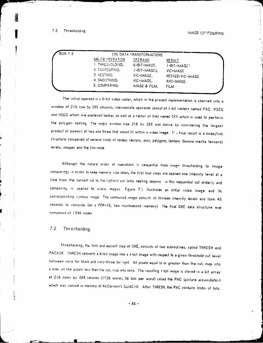
^m
I 7.2 Thresholding. IMAGE CC'ITOURING.
s BOX 7 2 CRE DATA TRANSFORMATIONS. MAJOR OPERATION OPERAND RESULT
1 THRESHOLDING: 6-BIT-IMAGE, 1-BIT-IMAGE", 2. CONTOURING: 1-BIT-IMAGES, VIC-IMAGE.
3- NESTING: VIC-IMAGE, NESTED-VIC-IMAGE 4. SMOOTHING: VIC-IMAGE, ARC-IMAGE. 5. COMPARING: IMAGE & FILM, FILM.
The Initial operand is a 6-bit video raster, which in the present implementation is coerced into a
window of 216 row by 288 columns; intermediate operands consist of 1-bit rasters named PAC, VSEG
and HSEG which are explained below, as well as a raster of links named SKY which is used to perform
the polygon nesting The magic window size 216 by 288 was derive by considering the largest
product of powers of two and three that would fit within a v,deo image. T! . final result is a node/lmk
structure composed of several kinds of nodes: vectors, arcs, polygons, lamtons (lamina inertia tensors)
levels, images and the film node.
Although the natural order of operations is sequential from imag« thresholding to image
comparing; in order to keep memory size down, the first four steps are applied one intensity level at a
time from the darkest cut to the lightest cut (only nesting dopend ,n this sequential cut order); and
comparing is applied lo whole images Figure 7.1 illustrates an initial video image and its
corresponding contour image. The contoured image consist-, of thirteen intensity levels and took 45
seconds to compute (on a PDP-IO, two microsecond memory) The final CRE data structure was
composed of 1 996 nodes.
7.2 ThreGholding.
Thresholding, tht first and easiest step of CRE, consists of two subroutines, called THRESH and
PACXOR THRESH converts a 6-bit image into a 1-bit image with respect to a given threshold cut level
botwoen zero (or black and r.ixty-throe for light. All pixels equal to or greater than the cut, map into
a one; all the pixels Ions than the cut, map into zero. The resulting 1-bit image is stored in a bit array
of 216 rows by 288 columns (1728 words, 36 bits per word) called the PAC (picture accumulator)
which was named in memory of McCormick's ILL1AC-III, After THRESH, the PAC contains blobs of bits.
-86
i^riki mm

FIGURE 7.1 - VIDEO IMAGE AND CONTOUR IMAGE. IMAGE CONTOURING.
87
iM mssi

f
I I I
'
7 3 Contourms IMAGE CONTOURING
A blob is defined *s "rook's move" connected; IM is «very bit of * blob can be reached by horizontal
or vertical moves from any other bit without having to cross a zero bit or having to make a diagonal
(bishop's) move Blobs may of course have hole«. Or equivaiently a blob always has one outer
perimeter polygon, and may have one, several or no inner perimeter polygons This blob and hole
topology is recoverable from the CRE data structure and is built by the nesting step
Next, PACXOR copies the PAC into two slightly larger bit arrays named HSEG and VSEG Then
the PAC n shifted down one row und exclusive 0R*d into the HSEG array; and the PAC is shifted right
one column and exclusive ORod into the VSEG array to compute the horizontal and vertical border bits
of the PAC blobs Notice, that technically this is the very heart of the edge fmder of CRE; namely,
PACXOR is the mechanism that converts regions into edges Edge tracing is the only operation CRE
performs Dn the 1-bit rasters; although Boolean image processing has caught the ey« of many vision
programmers (perhaps because it resembles an array automata or the game Life) one rapidly discovers
that raster operations alone are too weak to do anything interesting that can't already be done better
analytically in a raster of numbers or topologically m a node/link data structure
7.3 Contouring.
Contouring, converts the bit arrays HSEG and VSEG into vectors and polygons The contouring
itself, is done by a single subroutine named MKPGON, make polygon When MKPGON is called, it looks
fur the upper most left non-zoro bit in the VSEG array If the VSEG array is empty, MKPGON returns
a NIL However, when the bit is found, MKPGON traces and erases the polygonal outline to which that
bit belongs and returns a polygon node with a ring of vectors The MKPGON trace can go in four
directions: north and south along vertical columns of bits in the VSEG array, or east and west along
horizontal rows of the HSEG array The trace starts by heading south until it hits a turn; while heading
south MKPGON must check for first a turn to the east (indicated by a bit m HSEG); next for no turn
(continue south); and last for a turn to the west When a turn is encountered MKPGON creates a
vector node representing the run of bits between the previous turn and the present turn The trace
always ends heading west bound The outline so traced can be either the edge of a blob or a hole, the
two cas*s are distinguished by looking at the VIC-polygon's uppermost left pixel in the PAC bit array.
-88
^M

7 4 Polygon N«<tin| IMAGE CONTOURING
Th«r» ar« two compl«xi1i«s: centrist accumulition »rd dtKinkinj Th« contrast 0« a v«etor it
d.fmad as (QUOTIENT (DIFFERENCE (Sum of pixal valuas on on« sid« of th« v«ctor)(Sum of ptxal valu«s
on th« oth«r std« of th« v.ctor)) (laneth of Ih« vactor m pixals)) Sine« v«tor$ ar« always «ither
horizontal or v.rt.eal and ar« construad at bainf on th« craeKs batwaan p.xals; th« spacifiad
summations rtfar to th» pixals immad.ataly to aithar sid« ol th« v«etor Notic« that th.s d«fmition of
contrast will always |iv« a posit.va contrast for vaetors of a blob and naptiva contrast for th« v«ctors
of a hoi«
Th« contours that hav« just b««n tracad would appaar "sawtoothad" or "KmKy"; th« t«rms
"kinK", "sawtooth" and "jany" ara usad to axprats what saams to b« wrong about th« low«rmott l«ft
polygon in Figur« 7 2. Th« problem mvolvat doing somathing to a r«ctilin«ir quantizad s«t Of
s«gm«nts, to mak« its continuous natura mora avidant In CRE, th« jaggias solution (in th« subroutm«
MKPGON) m«r«ly positions th« turning locus diagonally off its grid point a httl« in th« dir«ction
(north«a$t, nor.hwast, southwast or soulhaast) that bisacts th« turn's right angla Th« distanc« of
d«kinK v«rni«r positioning is always lass than half a pixal; but graatar for bnghtar cuts and lass for
th« darkar cuts; in ordar to pr«s«rv« tha nastmg of contours Th« sawtoothad and th« d«kink«d
v«rsions of a polygon hav« tha sama numbar of vaetors I am vary fond J this dakinking algorithm
bacaus« of its incradibl« efficiancy; givan that you hava a north, south, «ast, wast polygon trac«
routm« (which handlas imaga coordinates packad row, column into on« word); th«n d«kinking r«quir«s
only on« mor« ADD instruction axecution par vactor !
7.4 Polygon Nesting.
Th« n«$ting probl«m is to d«cid« whathar ona contour polygon is within anothar Although «asy
in th« two polygon cas«; solving th« n«sting of many polygons with r«sp«ct to «ach othar b«com«s
n-squar«d «xp«nsiv« in «ith«r computa tima or in mamory spac« Th« n«sting solution in CRE
sacnficas m«mory for th« saka of graatar spaad and raquiras a 3IK array, callad th« SKY CRE's
accumulation of a proporly n«$tad traa of polygons dapands on tha ordar of thr«shold cutting going
from dark to light For «ach polygon thara ara two nastmg staps: first, tha polygon is placad in th«
89
^MM

I I I
FIGURE 7.2 - SAW TOOTH DEKINKING ILLUSTRATED. IMAGE CONTOURING
5 90
IAI mm^m
7 4 Poly ton N«tm| IMAGE CONTOURING
ITM of n«t«d polytons by »h« tubroutm« INTREE; »«cond, th» polyjon it placed in th« SKY array by
tha tubroutm« named INSKY
Th« SKY array n 216 rowt of 289 columnt of 18-bit pomUrt Th« nam« "SKY" cam« about
bacaut«, th« array us« to raprasant tha farthatt away ra|iont or background, which in th« cat« of a
robot vahicl« it th« r«al thy blu« Th« tky contamt vaetor pomtart; and would b« mor« «fficl«nt on a
virtual mamory machm« that didn't allocata unutad pagat of itt addrast tpac« Wh«r«as most
comput«rt hava mor« m«mory contamars than addratt tpaca; computar graphict and vition might b«
«ati«r to program in a mamory with more addratt tpac« than phytical tpac«; i«. an almott «mpty
virtual mamory
Th« firtt part of th« INTREE routm« Imdt th« turround«r of a givan polygon by tcannmg th«
SKY du« «att from th« upp«rmost lall pixel of tha givan polygon Th« SON of a polygon is always its
upper notl laft v«ctor Aft«r INTREE, th« INSKY routm« places pomtert to the vertical vectort of th«
giv«n ,'Olygon into th« tky array The second part of the INTREE routine checks for and fixes up th«
cat« whe« th« n«w polygon capturet a polygon that it already enclaved. Thit only happant whan two
or mor« l«v«lt of th« imag« have blobt that have holet. The next paragraph explains the arcane
details of fixing up the tree linkt of multi level hole polygont; and may be tkipped by «v«ryon« but
thos« who might with to impl«m«nt a polygon n«tt«r
Let th« giv«n polygon b« named Poly; and l«t th« turround«r of Poly b« called Exopoly; and
assume that Exopoly surrounds several enclaved polygons called "endo's", which are already in th«
n«st«d polygon tr«« Also, th«r« ar« two kinds of temporary lists named the PLIST and the NLIST
Ther« it on« 'LIST which is initially a list of all the ENOO polygont on Exopoly't ENDO ring Each «ndo
In turn hat an NLIST which it initially empty. Th« tubroutin« INTREE r«-teant th« tky array for th«
polygon du« «att (to th« l«ft) of th« upp«rmott l«ft v«ctor of «ach «ndo polygon on th« PLIST,
(Exopoly't ENDO ring). On tuch ^-scanning, (on behalf of tay an Endol), there ar« four cases: No
chnngr; th« scan raturnt Exopoly; which it Endol't original EXO. Po/y rnpturrt Hudol; th« tcan
raturnt Poly indicating that endol hat been captured by Poly. My brolhert fate; th« tcan hits an
«ndo2 which it not on the PLIST; which meant that endo2't EXO it valid and it th« valid EXO of «ndo!.
91
i
J

7 5 Contour SwM.Uo* 'MACE CONTOURING
My fntr drlayrH; th« ««n hits Ml »0002 which it ttill on tho PLIST; which MMM th«t •ndo2"$ EXO is
not y«t valid but *h«n discovered it wtH «Iso be Endol's EXO; so Endol is CONSed into Endo2,s NLIST
Wh.n an «ndo polyson's EXO has b««n rtJi!COv«r«d, th«n all th« polytons on that «ndo's NLIST ar«
also placod into th« polyton tre« at that plac« All of this link crunchint machm.ry taKas "lalf a pas« of
cod« and is not Iriquontly executed
7.5 Contour Segmentation.
In CRE the term tgmenlhg reters to the problem of breakinj a I-D manifold (a polygon) into
Simple functions (arcs) The segmentinf step, conve-ts the polygons of vertical and horizontal vectors
into polygons of arcs For the present the term "arc" means "linear are" which is a line segment
Fancier arcs: circular and cubic spline were implemented and thrown out mostly because they were of
no use to h.gher processes such as the polygon compare wh.ch would have to break the fancy arcs
bacK down into linear vectors for computing areas, inertia tensors or mere display buffers
Segmenting is applied to each polygon f a level To start, a ring of two arcs is formed (a
bi-gon) with one arc at the uppermost left and the other at the lowermost right of the given vector
polyROn Next a recursive maKe arc operation, MKARC, is appled to the two initial arcs Since the arc
given to MKARC is in a one to one correspondence with a doubly linked list of vectors; MKARC checks
to see whether each point on the list of vectors is close enough to the approximating arc MKARC
returns the given arc as good encugh when all the sub vectors fall within a given width; otherwise
MKARC splits the arc m two and places a new arc vertex on the vector vertex that was farthest away
from the original arc
The two large images in Figur«, 7 3, illustrate a polygon smoothed with arc width tolerances set
tt two different widths in order to show one recursion of MKARC The eight smaller images illustrate
the results of setting the arc width tolerance over a range of values. Because of the dekinking
mentioned earlier the arc width tolerance can be equal to or less than one pixel and still yield a
substantial reduction in the number of vectors it takes to describe a contour polygon.
92
^^

*»
IMAGE CONTOURING
FIGURE 7.3 - CONTOUR SEGMENTATION.

7 6 Related and Future Image Analysis IMAGE CONTOURING
A final .mporlanl detail is that the arc width tolerance is actually taken as a function of the
highest contrast vector found along the are; so that high contrast are« are smoothed with mceh smaller
are w.dth tolerances than are low contrast ares After smoothini, the contrast across each arc is
computed and the ring of ares replaces the nng of vectors of the g.ven polygon (Polygons that would
be expressed as only two ares are deleted)
7.6 Related and Future Image Analysis.
In general, robotic image analysis should consist of three step«: fir«», high quality p.ctures are
taken continuously in time and space; second, several iow level bulk operations (such a« correlation,
filtering, h.stogramming and thresholding) are applied to each .mage and to peirs of image«; th.rd, the
rasters are converted into imked 2-0 structures which are further amalgamated into connected 3-D
models It is clear to me that my present implementation only ha« fragile toy routine« where rugged
tools are needed Eventually, more kinds of .mage fe.tures and larger coherent structure« must be
included In particular, the contour mips should be bundled into regional mosaics and more features
should be woven into the node/link structure
Contour image processing is effectively surveyed by Freeman (74) who give« »he .rrontou«
„npress.on IM contour images are the best image representation (rasters and mosaic« «re equally
important) Contours are applied to recognition of silhouettes by Dudani (70) using moment« «imilar to
those explamed m the next chapter Finally, my own acquaintance with the contour image
representation wa« initially derived from papers by Zahn (66) and Krakauer (71)
-94
- -

8 0 Introduction to lm«g« Comparinj COMPARING.
I
I I
SECTION 8
IMAGE COMPARING.
8 0 Introduction to Imif« Compirinj
8 1 A Polygon Mitchmg Mtthod
8 2 Geomotnc Normilization ot Polygon»
8 3 Compare by Rtcursiv« Windowing
8 4 Related WorK and WorK Yet To Be Oone
8.0 Introduction to Image Comparing.
The image compare process is both the "kryitonr of ihr nrrh" it well as the "urnkru link of
f ihf rhnin' By comparing images, the 3-0 modeling and the 2-0 image processing are finally linked,
however as will be apparent the implementation to date demonstrates only a small part of what Is
i possible In the feecbacK perception design, there are thre« classes of compare operations:
verification, revelation and recognition which may be applied to each of the three Kinds of image data
I structures: raster, contour and mosaic The verify compare finds the corresponding entities between a
predicted image and a perceived im^ge for the saKe of calibration measurement and for the sake of
I eliminating already known features from further consideration In vision for industrial machine
assembly, calibration measurements suddenly seems to be the only kind of vision necessary in a
I relatively constrained factory situation The "-eveal compare involves finding the corresponding entities
in two perceived images, so that the location and extent of new objects can be solved. Finally, th«
recognition compare involves matching a perceived entity with one of a set of prototype entities
•95
^^

8,0 Introduction to Ir^s« Comparin| COMPARING
From th« vitw point ot modtlmj th« low«st ltv«l compart optntion should somthow b«
arranfcd to b« a on« to on« tsmplat« match rath«r than a multi dim«nsional statistical discrimination or
a Craph isomorphism l«st That is if th« «ntiti«t to b« match«d ar« incomm«nsurat«1 th« mod«l
d«sien«r c«n$ur«s th« mod«l that fnirrttd an unr«alistic pr«diction rath«r than th« patt«rn match«r
which cannot s«« a vaju« r«s«mblanc« Cl«arl/ this position should not b« taK«n to an «xtr«m« and th«
pr«s«nt syst«m could b« «nhanc«d by th« inclusion of an appropnat« coll«ction of traditional patt«rn
matchinj t«chniqu«s How«v«r1 two t«chniqu«s of comm«risuration that ar« naturally th« r«sponsibility
of a mod«l build«r ar« t«om«tric normalizat-on and topolojical s«tm«ntation G«om«trie normalization
mvolv«! «hmmatmi th« irr«l«yant |«om«tric diff«r«n<«s such as location, ori«nt«lion and seal«
TopolOfical s«tm«ntätion invoiv«s subdividinj a compl«K obj«ct into pi«c«$, (p«rhap8 «v«n canonical
pi«c«s) so that only simpl« small parts n««d b« match«d (that is th« compar« b«com«s r«eursiv«) Th«
r«maind«r of this chapUr «xplains a m«thod for matchmf structur«d imat«t consisting of polygons
Th« most original part of th« m«thod invo1v«s finding th« cor^spond«««, illustraUd in Figur« 8.1, for
polygonal figur«s that fission O' (us« from on« imag« to th« n«xt
FIGURE 8.1 - EXAMPLE OF POLYGON FUSION COMPARE.
96 -
^rti

8 1 A Polyjon Mitchlnj Method COMPARING
8.1 A Polygon Matching Method.
Th« imajo compar» process m CRE, conneeti the polyjons md vector« of one image with
correipondmg polygon« and vector« of another imag» CRE'« compare «olves the problem of
correlating polygons between two iMItr images and is composed of four step«:
1 Compute polygonal lamina inertia tensors, Inmirn nndr*
2 Compare and connect polygons one to one at corresponding level« of the nested polygon tree
3 Compare and connect polygons two to one at corresponding level« of the nested polygon tree
4 Compare and connect vertices of connected polygon« u«ing recur«ive windowing
First, the lamina inertia tensor nodes (called (nminr«) of all the polygons of an image are
computed A lamlen node contains the center of mas« a« well as the tensor of a polygon The maanmg
of the inertia tensor is that it characterizes each polygon as a rectangle of a rertam length and width
at a particular location and orientation; and of further importance such inertia tensors can be added to
characterize two or more polygons by a single rectangle It it the lamten rectangles that provide a
basis for normalization
Second, all the lamtens of the polygons of one level of the first image are compared with all the
lamtens of the polygons of the corresponding level of the second image for nearly exact match The
potentially (M»N/2) compares is avoided by sorting on the center of mas« locations. In CRE, which i«
intended tor comparing sequences of picture« of natural scenes; match for center of mass location is
tested first and most strictly, followed by match for inertia. Pointer« between matching polygons are
placed m two link positions of the polygon nodes and the polygons are considered to be matched.
Third, all the unmated polygons of a level are considered two at a lime ano a fusion lamten node
for each pair is made The potentially (N«N/2-N) fusion lamten« are avoided because there it a
maximum possible unmated inertia in the other image; if there are no unmated polygons in one image
then the extra polygons of the first image can be ignored. In the event where there are unmated
polygons in corresponding levels of the two images, the multi-polygon fusion lamter. of one are
compared with the single polygon lamten of the other. The fusion (fission) compare solves the rather
•97
mm

8 2 G«om«lric Normalization o« Polygons COMPARING
nasty probl.m. of ImKmt two contour polyROnt of on« mtf with a lingl« contour polyton in th« n«xt
imae«
Fourth, th« v«rtic«t of mat«d polyjont ar« in turn compar«d and mat«d To «tart a v«rt«x
compar«, th« v«rtic«i of on« polygon .-« transUt«d, rotatad and d.latad to g«« that polygon'« lami«n
r«ctanel« co...cid«nt with its mat« (or rnaUs) Concaptually, «ach v«rt«x of on« polygon is eompar«d
with «ach v«rt«» of th« oth«r polygon(B) and th« mutually clos«st v«rtic«s (clos«r than an «psilon) ar«
eonsid«r«d to b« mat«d Actually th« pot«ntial (N*M) compares ar« avoided by a r«cursiv« windowing
sch«m« similar to that us«d in hidd«n Im« ol.mmation algorithms Th« compar« «x«cuiion taK«s l«ss
th^n a s«cond on imag«s such as th« pump bas« (Figuras 0 3 and 0 4) blocks (Figur« 8 1) and a doll
(Figur« 8.2) Th« doll's silhou«tt« is h«adl«ss wh«n vi«w«d from th« bacKsid« b«caus« its hair is black
FIGURE 8.2 - EXAMPLE OF VERTEX MATCHING.
8.2 Geometric Normalization of Polygons.
Th« lamina in«rtia Unsor of a polygon with N sides i. compuUd by summation ov«r N frap«20id«.
Th« trap«20id corresponding to «ach sid« is form«d by dropping p«rp«ndicul«rs up to th« top of th«
iNMM fram«; «ach such trapazoid consists of a r«ctangl« an a right tnangl«; sine« th« sides of
98
- -

8.2 Gaomstric Normdization of Poi/gons COMPARING
polrROns art directed vector; the areas o< the tmngles and rectangles can be arranged to take
positive and negative value", '.uch that a summation will describe the interior region of the polygon as
positive The equation', necc.iary for computing the lamina inertia tensor of a polygon were derived
from material in (Golditem 1950)
RECTANGLE'S LAMINA INERTIA TENSOR ABOUT ITS CENTER OF MASS MXX •- B*B*AREA/I2; (B HEIGHT IN ROWS). MYV - A*A*AREA/I2; (A WIDTH IN COLUMNS) MZZ •■ MXX • MYY; PXY - 0;
ORIENTED RIGHT TRIANGLE'S LAMINA INERTIA TENSOR ABOUT ITS CENTER OF MASS MXX * B«B*AREA/I8: (B HEIGHT IN ROWS) MYY - A«A*AREA/18; (A WIDTH IN COLUMNS) MZZ «■ MXX ♦ MYY; PXY - -A*B*AREA/36;
SUMMATION Pf LAMINA INERTIA TENSORS AREA - XCM - YCM - MXX «- MYY - PXY -
(AREA: ♦ AREA2); (AREA1*XCM1 • AREA2 * XCM2) / AktA, {'7EAI * YCMI • AREA2 « YCM2) / AREA; MXX! ♦YCMI*YCMi«AREAl .MXX2 ♦YCM2*YCM2«AREA2 -YCM«VCM*AREA; MYY1 .XCMI«XCMi«AREAl •MVY2 ♦XCM2«XCM2*AREA2 -XCM«XCM«AREA; PXY1 -XCMUYCMUAREAI ♦PXY2-XCM2«YCM2«AREA2 «XCMmYCMatAREA;
ANGLE OF PRINCIPLE AXIS The angle of the principle axis, PHI, lies in the interval -n/2 to n/2
PHI *• 0 5*ATAN(2*PXY/(MYY-MXX)); PXY •- 0 5«(MYY - MXX)«TAN(2«PHI);
TRANSLATION OF LAMINA INERTIA TENSOR AWAY FROM CENTER OF MASS MXX" - MXX ♦ AREA*DY«DY; MYY' ♦• MYY • AREA«DX*DX; PXY' •- PXY - AREA*DX*DY;
ROTATION OF LAMINA INERTIA TENSOR ABOUT CENTER OF MASS. C - COSINE(PHI); S - SINE(PHI); MXX' - C«C*MXX ♦ S«S*MYY - 2«C*S*PXY; MYY' •- C«C*MYY • S*S*MXX ♦ 2«C*S«PXY; PXY' - (C*C - S«S)*PXY • C*S«(MYY - MXX);
99
^^

^"
^
8 4 Ralatad Work and Work Y«t To B« Don« COMPARING
8.3 Compare by Recursive Windowing.
Th« final step m th« CRE polyton match (Section 8 1) it to link th« corresponding v«rtic«t
b«twaan two t«on>«tncally normali2«d polyton» (or t«tt of polyfOns) using a n«ar«t ntijhbor
crit«rion Th# n«ar»jt neighbor« ar« found by r«curjiv« windowing, initially all 1h« varticat ar«
puthad into ona larga window which it tubtaquantly tplit until thara war« faw anough varticat
containad in tha window to allow axhauttiva comparing To maka Ihit windowing tachmqua applicable
to tha naarast naighbor problam a dittanca cntanon, drlia, hat 10 ba daclarad to that tha wmdowt
ovarlap by that amount Consaquantly tha windows ara no longar disjoint ractanglat, but ara rathar
boxat with roundad cornart, tha smallast postibla window bamg a circla with radius, drlia Th«
racurtiva windowing tachmqua is astontially a two dimantional partition sort, tha tachmqua can b«
ganoralizad for comparing adgis and othor ontitiat in 2*D or highar dimantiont.
8.4 Related Work and Work Yet To Be Done.
To complata tha visual faadback tystam, thara ramamt yat to ba written an imaga compare that
uses both raster basad and polygon basad tachniquat Tha two kindt of compares are symbiotic in that
the polygon compare could aim the raster correlator alleviating the need to do bulk correlation over
wide areas, and the raster correlator could verify and improve the measurement of corresponding
vertex loci At Stanford, image comparison by raster correlation techniques it begin worked on by
Ouam(7l), Hannah and Morevac Another approach to comparing polygons is to examine their
curvature, the curvtturi of a polygon can ba expressed as a parametric function of arc length; two
such functions can be ;iormalize'< and alligned and diffarancec; using statistical techniques (Zahn 66)
100
mm

I 9.0 Introduction to Locus Solving LOCUS SOLVING
SECTION 9.
CAMERA AND FEATURE LOCUS SOLVING.
9 0 Introduction to Locus Solving
9.1 An Eight PanmaUr Camera Modal
9 2 Camera Locus Solving: On« Viaw ot Thra« Points
9 3 Objact Locus Solving: Silhouatta Cona Intartaction.
9 4 Sun Locus Solving: A Simple Solar Ephamarit.
9 5 Ralatad and Futura Locus Solving Work
9.0 Introduction to Locus Solving.
There are thraa kinds of locus solving problems in computer vision: camera locus solving,
feature locus solving and sun 'ocus solving Camera solving is routinely attempted in two ways: using
one image the 2-D image loci r f a set of already known 3-D world loci (perhaps points on a calibration
object) are measured and a Ct-^era model is confuted; or using two or more images a set of
corresponding landmark feature pom's are found among the images and the whole system is solved
relative to itself After the camera positions are known, the location and extent of the objects
composing the scene can be found using parallax (motion parallax and stereo parallax) Parallax is the
principal means of depth perception and is the alchemist for converting 2-D images into 3-D models
After the camera and object positions are known to some accuracy, the nature and location of light
sources might potentially be deduced from 'he shines and shadows in the images However, in outdoor
situations the primary light source is the sun, whose position in the sky can be computed from the time,
date and latitude by means of a simple solar ephemeris routine
I 101 -
- -

mm
9.1 An Eifht P«r«m«Ur C«m«r» Mod«l LOCUS SOLVING.
9.1 An Eight Parameter Camera Model.
In GEOMED md ORE ItN b«sic cimtra mod«l is ip«c.fi«d by «nht p«rim«t«ri. Th«r« ar* Ihr««
MTMMton for th« l«n« c«nt«r locit.on of th« c.m«ri: CX, CY, C2; «hr«« p«r«m«1«r« for th«
ori«nti1ioni WX, WY, WZ; md »wo pirim«t«ri for «h« proj«e1ion rit.oi: th« aspect ratio, AR; and th«
focal ratio, FR Th« location is |iv«n in world coordmaUs and th« oriontation is sp«cifi«d by a rotation
v«c»or whos« dir«ction |iv«i an axis and whos« magmtud« |iv«s rotation which wh«n applied to a s«t
of thr«« ax«s unit v«ctors yi«ld$ » s«t of unit v«ctors that d«t«rmin«s th« cam«ra,s coordmat« syst«m
By conv«ntion th« p. -K.pal ray of th« cam«ri is parall«! to th« 2 axis unit v«ctor and it n«fativ«ly
dir«ct«d Th« cam«ra rast«r is allitnad such that th« rows (vidicon scan lines) ar« parall«! to th« X unit
voctor and th« columns ar« parall«! to th« Y unit v«ctor
Th« asp«ct ratio, AR, is th« ratio of width, PDX, to haifhl, PDY, of a ting!« vidicon tampl« point
call«d a pix«!: AR » PDX/PDY Th« focal ratio, FR, is th« ratio of th« focal plan« distanc« to th« h«ifht
of a smtl« pix«l: FR • FOCAL/PDY Th« typical valu« of th« «sped ratio is about on«, and th« typical
valu« of th« focal ratio runs from 300 to 3000
Th« actual physical siz« of th« digital rastar of a t«l«vision vidicon is on th« ordor ol 12
millim«1«r$ wid« by 8 millim«t«rs high with approximataly 512 lin«s of pot«ntially 512 pix«ls per lin«.
How«v«r, a standard t«l«vition scans its rasUr in two phas«s (odd rows in on« phas«, «v«n rows in th«
n«xt) so that a on«-phas« pix«l is approximat«ly 40 microns by 40 microns (rathar than 20 by 20) B«,
contrast, th« con«s and rods in a human «y« ar« 1 and 2 microns in diam«t«r r«sp«ctiv«ly
Th« aspact ratio and th« focal ratio can b« m«asurad individually using a tph«rical calibration
objoct. I hav« used plastic toy balls and billiard balls, billiard ball radius RBB.2 125". Th« p«rsp«ctiv«
projoction of a sph«r« is an «Hips« and th« ratio of th« apparent width to haight of th« «Hips« of a
tph«r« that naarly fills th« vi«wing scr««n is th« aspact ratio. To maasur« th« focal ratio, mount th«
tph«r« on a stick and moasura its apparent radii (rl and r2) at two positions that ar« approximataly
along th« camera's principal axis a measured distance, DZ, apart. Then then the focal ratio FR •
102
^^ MK4

■^
I I 9 1 An Eight Pirn Mr Camera Model LOCUS SOLVING
DZ«rl*r2/(R*(rl-r2)) which can be thought of as the FOCAL plane distance in pixels The beauty o<
this is that a naive measuring method yields results as good as measurements obtained by more
elaborate methods such as principal axis relaxation of a camera model in numerous variables (Sobel 70)
and Pmgle unpublished
Camora Resolution The focal ratio description allows one to have a firm numerical intuition of
camera's spatial resolution in the object space The smallest distance interval, DELTA, a earner« can
measure at a given range, RNG, is merely the ratio of range to TR: DELTA«RNG/FR The «rcian of th«
reciprocal of the focal ratio ARCTAN(1/FR) is the angle subtended by a tingle pixel
Lens Center Irrelevancy Theorpm The actual location of the prineioal axis of the lens in the
image plane ii irrelevant boceu-.e Iho effect of deviation from the true center is equivalent to rotating
the camera Many camera modelr.ts worry needlessly about the exact location of the camera lens
center; the angular error, ANGCPR, of a pixel X units from the center of the image of a camera
modeled with a lens center that is wrong in the X direction by 0 pixels is .jiven by the following
expression:
ANGER" i ARCTAN(X/FR) - ARCTAN((X»0)/FR) - ARCTAN(Q/FR)
Which for the physical parameters of the television hardware at Stanford in 1974; means that the lens
center can be allowed to wandor by tens of pixels from its true position without causing a pixel of
error at the edge of the image, (allowing that one camera model is alhgned on the same feature by
rotation as the camera that defines a good lens center)
I I 103
^^
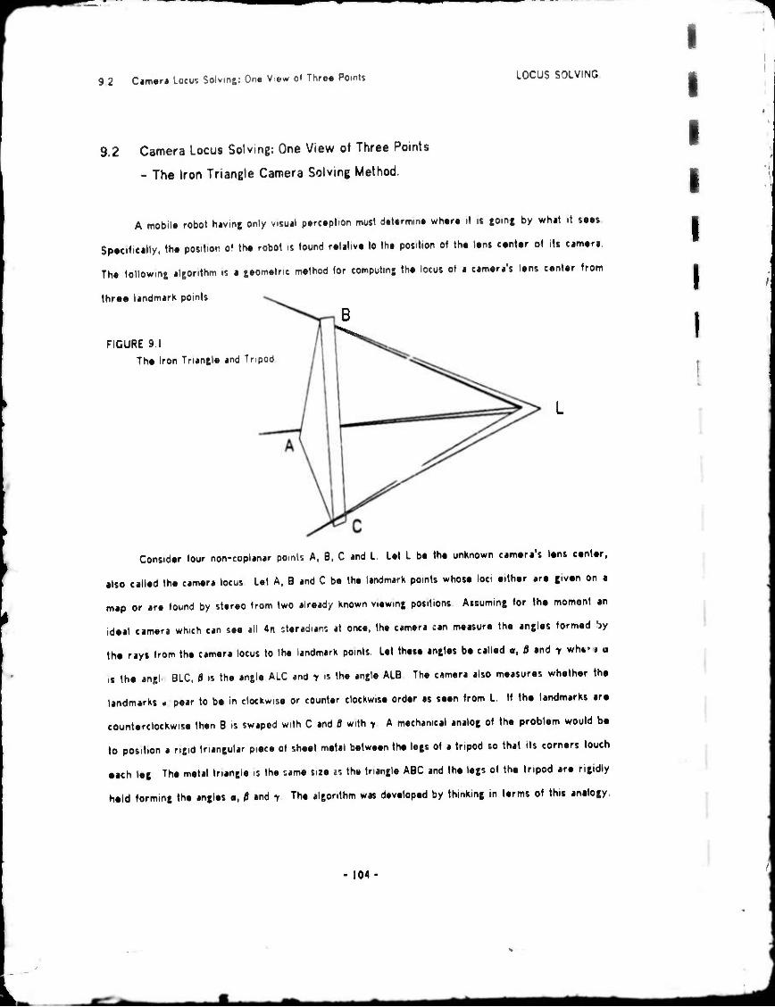
^»
9 2 C«m«ri Locus Solving: On« V.ew o» Thro« Points LOCUS SOLVING
9.2 Camera Locus Solving: One View of Three Points
- The Iron Triangle Camera Solving Method.
A mobil« robot hiving only vitual p«rc«ption must d«t«rmin« wh«r« it it tomt by what it MM.
Sp«cifieilly, th« position o« Ih« robot is tound r«l»tiv« to th« position ot th« l«ns c«nl«r ol its CMMTt.
Th« »ollowmg algorithm is a geometric method «Or computing th« locus ot a cam«ra,s l«ns center from
three landmark points.
FIGURE 9,1
The Iron Triangle and Tnpod
Consider (our non-coplanar points A, B, C and L. Let L be the unknown camera's lens center,
also called the camera locus Let A, B and C be the landmark points whose loci either are fven on a
map or are found by stereo from two already known viewing positions Assuming for the moment an
ideal camera which can see all 4n steradians at once, the camera can measure the angles formed by
the ray« from the camera locus to the landmark points. Let these angles be called a, 8 and y wh*» t a
it the angl BLC, ß is the angle ALC and y is the angle ALB The camera also measures whether the
landmarks • pear to be in clockwise or counter clockwise order as seen from L If the landmarks are
counterclockwise then B is swapod with C and 6 with y A mechanical analog of the problem would be
to position a rigid triangular piece of sheet metal between the logs of a tripod so that its corners touch
each leg The metal triangle is the same size as the triangle ABC and the legs of the tripod are rigidly
held forming the angles a, $ and y The algorithm was developed by thinking in terms of thit analogy.
I I I I I I I
104
mm
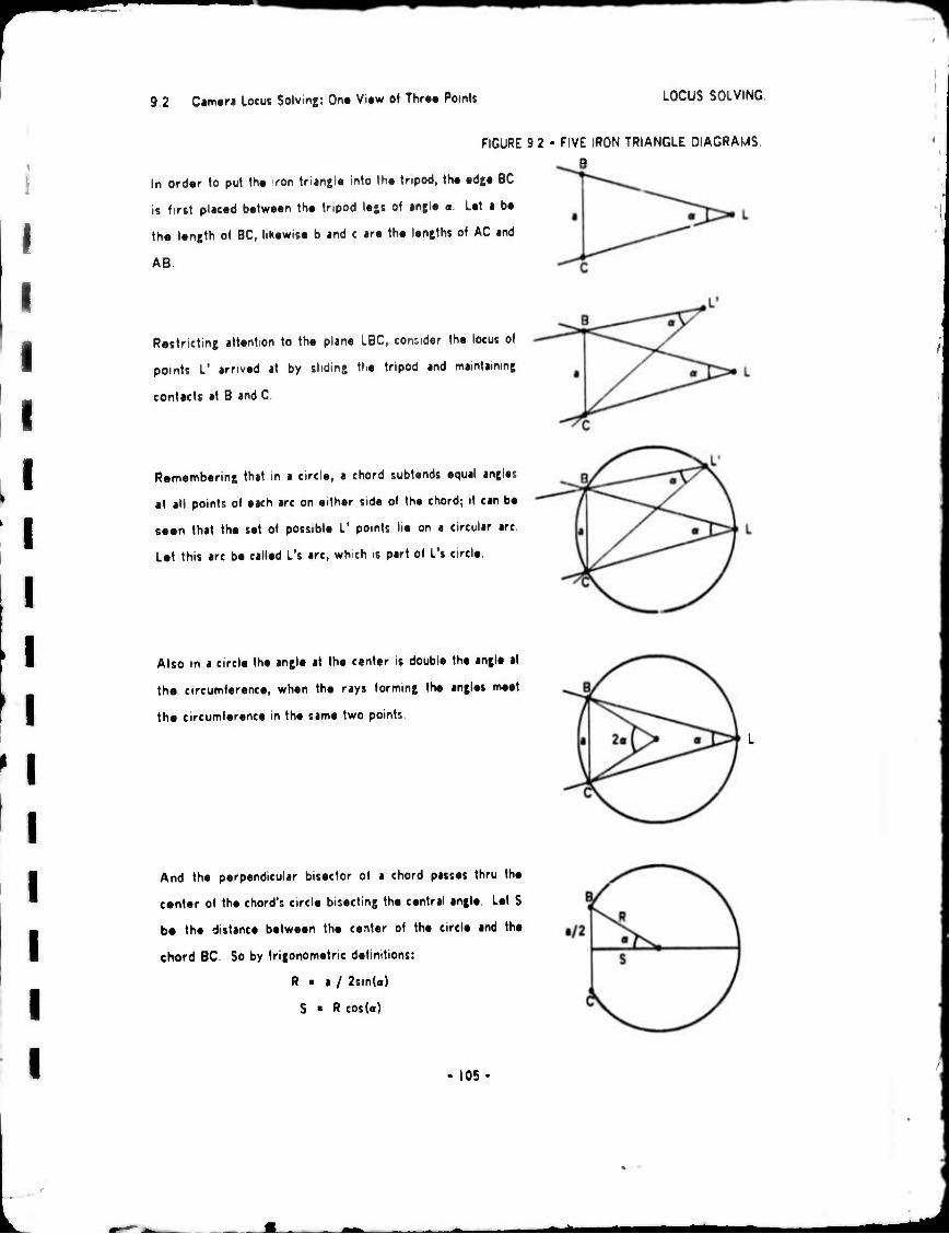
9.2 Cam«r» Locus Solvmt: On« Vi»w of Thr»« Pomli LOCUS SOLVING.
FIGURE 9 2 • FIVE IRON TRIANGLE
In ord«r 1o pu» th« ron Irungl» mlo th« tnpod, 1h« »df BC
is first pl«c«d b«»wMn th« tr,pod le;s of «ngl« a. L«t i b«
th« l«n|th of BC, IIK«WIS« b «nd c «r« th« l«njth$ of AC snd
AS
R«strictin6 attention to th« plan« LBC, consider th« locus of
points L* •rriv«d «t by sliding th« tripod and mimtiinint
contacts at B and C
DIAGRAMS
R«memb«ring that in a cird«, a chord subtends «qual angles
at all points of each arc on either side of the chord; it can be
seen that th« s«t of possible L' points lie on a circular arc.
Let this arc be called L's arc, wh ch is part of L's circle.
Also in a circle th« angl« at th« cent«r is doubl« th« angl« at
th« circumference, when the rays forming the angles meet
th« circumference in th« sam« two points
And th« perpendicular bisector of a chord passes thru th«
c«nt«r of th« chord's circl« bi5«cting th« c«ntral angl« Let S
be th« distanc« b«tw««n th« c«nt«r of th« circl« and th«
chord BC So by trigonometric definitions:
R ■ a / 2sin(a)
S ■ R cos(a)
• 105

92 Cimtra Locus Solvmj: On« Vi«w ol Thr«« Point» LOCUS SOLVING
var
Tha posit.on of L on its »re m th« plan* 8LC c«n b« ««pr^sstd .n t.rms of on« p«ram«'r.c
iabl« om«e* w. wh«r« w .5 th« count«r clockw.s« MgHUr displac«m«nt of L from th« p«rp«ndicular
bi$«ctor «uch that for wn-a, L .$ at B and for u*a-n. L is at C By spmnmu th« iron tr.antl« «bout th«
•xit BC, th« v«rtM A sweeps a c.rtl« L«t H b« th« radius of A's ere!« and l«t D b« th« d1r«ct«d
dotanc« b«tw««n th« c«nt«r of A's circl« and th« midpoint of 5C. By Trnonom«tric relations on th«
tnangl« ABC:
COS(ACB) • (aT2 ♦ bT2 - cT2)/2ab SIN{ACB)« SORTd -C0S(C)T2)
H • b SIN(ACB) D « b COS(ACB) - a/2
Now eontid«r th« third !«( of th« tripod which form« th« angl«« tf and > Th« third ieR
int«rs«ct« th« BLC plan« at point L and «xtonds into th« appropnat« halfspac« «o that th« landmark
points app«ar to b« in clockwis« ord«r as MM from L Lot A' b« th« third I«»'« point of int«rs«ction
with th« plan« contaimnt A's circl« Lot th« distanc« b«tw««n th« point A1 and th« c«nt«r of A's circl«
l«ss th« radius H of A's lircl« b« call«d "Th« Gap" Th« e*p's valu« is n«8at.v« if A' falls within A's
circl«. By constructin8 an «xpressior for th« valu« of th« Gap as a function of th« param«tric vanabl«
w, a root solvmt routin« can find th« H for which th« gap is 2«rO thus d«t«rm1nin6 th« onontation of
th« tnanil« with r«sp«ct to th« tnpod and Ml turn th« locus of th« point L in space
Using vector fOtvWy, plac« an origin at th« midpoint of BC, «stablish th« unit y-v«ctor j
pointing towards th« v«rt«x B, let th« plan« BCL b« th« x-y plan« and onont th« unit x-v«etor i
pomtmc into L's halfplan« For right handodnoss, s«t th« unit z-v«ctor K to i cross j In th« n«wly
d«fin«d coordinat«s points B, C, and L b«com« th« v«ctors:
B » (-s, •a/2, 0); C • (-s,-a/2,0) L • (R coslw), R sin(w), 0)
Introducing two unknowns xx and zz th« locus of point A' as a vector is:
A' • (xx, D, zz)
106
^^i wm

I I \
I
1
I
I I
I I I I
9.2 Cim«r« Locus Solving: On« Vi«w of Thr«« PoinU LOCUS SOLVING.
Th« vtelors corresponding to the legs of the tripod ire:
LB « B - L « (-s-Rcos(w), ••/2-Rsin(w)l 0)
LC » C - L » (-s-Rcos(w), -•/2-R»in(w), 0)
LA » A'- L • (xx-Rcoslw), D-Rsmlw), zz)
Since the third leg forms the angles B «nd y:
LA LC * |LA| |LC| cosW)
LA LB « |LA| |LB| cos(>)
Solving each equation for |LA| yields:
|LA| • (LA LC)/|LC|cos(tf) • (LA LB)/|LB|co«(ir)
Multiplying by |LB| |LC1 cos iß) cos b) t,v":
(LA LC)|LB| cosi-y) » (LA LB)|LC| cos(fl)
Expressing the vector quintites in t»-ms of their components:
|LB| » sqrt((-S-Rc05(w))T2 • (•»/2-Rsin(w))T2)
|LC| « sqrt((-S-Rcos(w))T2 ♦ (-i/2-Rsin(w))T2)
LA LC » (xx-Rcos(w))(-s-Rcos(w)) • (D-Rsm(w))f-i/2-R»m(w))
LA LC ■ (xx-Rcos(w))(-s-Rcos(w)) • (D-Rsin(w))(»i/k-Siin(w))
Substituting: ((xx-Rcos(w))(-s-Rcos(w)) ♦ (D-Rsin(w))(-«/2-Rim(w))) |LB|cos(7)
((xx-Rcos(w))(-s-Rcos(w)) • (D-Rsin(w))('«/2-R«in(w))) |LC|cosW)
The previous equation is linear in xx, so solving for xx:
xx = P/Q ♦ Rcos(w)
where P « (-s-Rco$(w))(lLB|cüs('r) - |LC|cos(fl))
Q . (D-Rsin(w))(('a/2-Rsin(w))|LC|cos(fl)
- (-a/2-Rsin(w))|LB|cos('r))
I The unknown zz can be found from the definition of |LA|
|LA| • sqrU (xx-Rcos(w))T2 ♦ (D-Rsin(w))T2 ♦ zzt2)
so zz « sqrt( 1LA|T2 - (P/0)T2 - (D-Rsin(w))T2)
and since:
|LA| • (LA LC) / |LC|cos(fl)
The negative values of zz are precluded by the clockwise ordering
of tha landmark points Thus the expression for the Gap can be formed:
GAP • sqrU (XX.S)T2 • zzT2 ) - H
- 107
mm

9 2 Cimeri Locus Solving: One View ol Three Points LOCUS SOLVING
As mentioned above, when the gap is zero the problem is solved r e the locus ot A' then must
be on A's c.re.e. «o the triangle touches the third leg The gap fun. jn loot-.s like • cubic on its
interval [e-n.n-a] which almost always has just one lero crossing
Having found the locus of L in the specially defined coordinate system all that remains to do i* to
solve for the components of L m the coordinate system that A, B and C were given Thi« can be done
by considering three vector expressions which are not dependent on the frame of reference and do
not heve second order L terms, namely: (CA dot CD; (CB dot CU| and ((CA x CB) dot CD Let the
locus of L m the given frame of reference be IX,V,Z) «nd let the components of Iho points A, B end C
be (XA.YAJA), (XB.YB^B) and (XC.YCZC) respectively Lilmg all four points in both frames of
reference:
A « (xx, 0, n) • (XA, YA, ZA) B « (-s, '»12, 0) « (XB, YA, 2A) C • (-s, -a/2, 0) • (XC, YC, ZC) L • (Rcos(w),Rsin(w),0) « ( X, Y, Z)
Evaluating the vector expressions which are invariant: CA . A - C • (XA-XC YA-VC, ZA-ZC) CB-B-CIO.a.O) ■ (XB-XC, YB-YC, ZB-ZC)
CL - L - C » (Rcos(w).s.Rsin(w).a/210) • ( X-XC, Y-YC, Z-ZC)
The aot products are: CA CL • (xx.S)(Rco5(w)«sHD»a/2)(Rsin(w)«A/2)
. (XA-XCKX-XC) • (YA-YC)(Y-YC) • {ZA-ZC)(Z-ZC)
CB CL ■ a(Rsin(w) ♦ a/2) . (XB-XCKX-XC) ♦ (YB-YC)(Y-YC) ♦ (ZB-ZC)(Z-ZC)
The cross product is: (CA x CB) CL » -a zz(Rcos(w) • s)
. ((YA-YC)(ZB-ZC) - (ZA-ZC)(YB-YC)) (X-XC) - ((XA-XCKZB-ZC) - (ZA-ZC)(XB-XC)) (Y-YC) ♦ ((XA-XC)(YB-YC) - (YA-YC)(XB-XC)) (Z-ZC)
The last three equations are linear equations in the three unknowns X, Y and Z which «re reedily
isolated by Cramer's Rule The whole method has been implement in auxiliary programs LSIV3P and
QBALL which calibrate a camera with respect to a turntable for the sake of the silhouette cone
intersection demonstration in Section 9 3
108 -
- —
I I I
!
I
9 3 Object Locus Solving: Silhouette Con« InUrstclion LOCUS SOLVING
9.3 Object Locus Solving: Silhouette Cone Intersection.
After the camera location, orientation and projection are Known; 3-D object models can be
. constructed The silhouette cone intersection method it a conceptually simple form of wide angle,
stereo reconstruction The idea «rose out of an original intention to do "blob" oriented visual model
I acquisition, however a 2-0 blob came to be represented by a silhouette polygon and a 3-D blob
consequently came to be represented by a polyhedron The present implementation requires a very
favorably arranged viewing environment (white objects on darK backgrounds or vice versa); application
to more natural situations might be possible if the necessary hardware (ard software) were available
for extracting depth discontinuities by bulk correla'ion F. Ihermo.e, the restriction to turntable
rotation is for the sake of easy camera solving; this restriction could be lifted by providing stronger
feature tracking for camera calibration
Figure 9 3 shows lour video images dnd the corresponding silhouette contours of a baby doll on
a turn table Figure 9 4 is an overhead view o* the four silhouette cones that were swept from the
contours, the cncle In the middle of Figure 9 4 is the turntable Figure 9 5 gives three views (cross
• yed stereo pairs) of the polyhedron that resulted by taking the intersection of the four silhouette
cones Like in th<» joKe about carving a statue by cutting away everything that does not look like the
subject, the approximate shape of the doll is hewed out of 3-D .pace by cutting away everything that
falls outside of the silhouettes A second example of silhouette cone intersection is depicted in Figure
9 6; the model was made from three silhouettes of the horse facing to the left which can be compared
with an initial video image and a final view of the result of the horse facing to th« right - • plausible
(maximal) backside has been constructed that is consistent with the front views.
The silhouette cone intersection method does indeed construct concave objects and even objects
with holes m them - what are missed ^re concavities with a full nm, that is points on the surface of the
object whose tangent pl*ne cuts the surface in a loop that encloses the point
109
^^ta

FIGURE 9.3 - FOUR VIEWS OF A BABY DOLL. video images silhouette contours
„mi! ., ■, ■•.iMf.>i«.>ni>|Mi"«)i.p ftifi
\l<"
I lluini'"-1'
1
■H i I' .1 ■MIL
'. ■' ' ;...■. rM.||.
I'li -I -
f ■■'■
iltrr j i IM
■'ii
. »uiiiiiiiii;"
iiirpnii -
i
'"'"'' ilrll .l||||.
I I
UüiuyiiMiiiMiinui1 ■ Hill I iibM iLttlUI
- 110
^^i

^^ n
I I I I
FIGURE 9.4 - FOUR TURNTABLE SILHOUETTE CONES. ...as viewed from above.
I
1
111
mm

FIGURE 9.5 - RESULTS OF SILHOUETTE CONE INTERSECTION
Front View.
Rear View.
Top View.
112-
^fe

i l
I
FIGURE 9.6 - HIGH HORSE SILHOUETTE CONE INTERSECTION
11.11
il! IM 1
-•- •> "^i;|" i"" r ii' 11| »'"I ^t"—YH
•lilr " I
I 'HI 1
n1
% ■
I,,, •, I, /'
ij " |H "; H
I'l'il i« i ,1, ,.;■■■. . ■ '•' •mi lllilll |,.'l(Miuujhlillilii.llmiilLiiili Uiiiüitl . "Uitoir i uiuiUiiliiliiui.ilHililiiiM.,luiill.uuÜll
113


I I 9 5 R.lalod «nd Futur« Locus Solvmj Work. LOCUS SOLVING
9.5 Related and Future Locus Solving Work.
* Th« cim«ra solvmt problem is discuss.d in Roberts (63), Sob«! (70) and 0u«m (71), I hav«
always dislik.d th« many dimensional hill chmbmt approach to cam«ra solvinj and hav« sought mor«
C«om«trie «nd intuitiv« solutions to th« probl.m Although th« bulk of this chapt«r conc«rn«d cam.r«
solving using on« vi«y; ot thr«« points th« multi vi«w c«m«ra calibration is probably mor« important to
continuous imag« proc«ssint
»
115-
^^

10.1 Rtculit: Accomplishments and Onjin*! Contributions RESULTS AND CONCLUSIONS
(
I I I
SECTION 10.
RESULTS AND CONCLUSIONS.
10 1 Results: Accomplishments and Original Contributions
10 2 Critique: Errors and Ommissions
10 3 Sucsestions for Future Work
10 4 Conclusion
10.1 Results: Accomplishments and Original Contributions.
I
At a regular feature in a PhD dessert.tion, it is required to state explicitly what has been
accomplished and what is original Some of what has been accomplished is itemized in box 10 1; with
the so called nrininnl ronirilmiinin marked by asterisk: Each of the accomplishments has been
elaborated in the indicated chapter
/ BOX 10 1 ACCOMPLISHMENTS AND ORIGINAL CONTRIBUTIONS
v
0 The Geometric Feedback Vision Theory
•1, The Winged Edge Polyhedron Representation
*2 The Euler Primitives for Polyhedron Construction
3 The Iron Triangle Camera Locus Algorithm
»4 The OCCULT hidden line elimination algorithm
*5 The Polygon Nesting Algorithm
*6 Ti.e Polygon Dekmkmg Method
7 The Polygon Segmenting Method
8. The Polygon Comparing Method
*9 Silhouette Cone Intersection
Chapter 6
Chapter 2.
Chapter 3
Chapter 9.
Chapter 4
Chapter 7
Chapter 7
Chapter 7
Chapter 8
Chapters 5 and 9
As a whole, the system described in this thesis is the third of its kind, succeeding the systems of
Roberts (1963) and Falk (1970) Although, the modeling routines of the present system are
considerably more sophisticated than were those of its predecessors; improvement in the visual
analysis routines is less dramatic and more open to question. The present image analysis differs from
116
^^ta

^»
10 1 R«ulU: Accomplishmenls and Original Confnbul.ons RESULTS AND CONt LUSIONS
th« ••rli«r sysUms In that «nnphasis is plK«d on th« us« of mullipl« imaj« for lh« sake of parallax
dapth parcapfion and in lhat savaral spatially connacled ima|a raprasantations art combinad (contour
imata, mosaic imaga and raslar MMg«) to prasarva tha structura of tha scana throufh faatur«
attraction rathar than followmt tha earlier paradum of axtradmt features from the imafa plecameal
and attempting to splice them together afterwards
As a design theory, the present work can be compared with earlier work by comparing tha
block diagrams The charctenstically circular feedback vision mandala like diagrams appear in (Falk)
Figure 4-7, page 78; (Grape) Figure 12.1, page 242; (Tenenbaum) Figure 1.13, page 43; as wall as in
this work Figure 6.1, page 70 The feedback mandala is conspicuously absent in the best of th«
stimulus-response visual parsing work, (Waltx), as well as in statistical recognition work, (Duda ard
Hart). Tha important ideas depicted m the feedback vision n-endala are the duality of the simulated and
physical worlds, tha duality of description and verification, tha dua sm of camera and body locus
solving, and tha dual opposing flows of predicted and perceived nages along a hiaracry of
commensurate abstractions Tenenbaum's figure illustrates the basic feedback loop in the immediate
vicinity of the visual sensor The diagrams of Falk and Grape are similar mirrors of the overall system
design of the Stanford Hand/Eye group (1969 to 1973) under tha leadership of Professor Jerome
Feldman The two diagrams depict an array of relevant boxes (camera solver, edge finder, world
modeler and so on) all sending messages to each other under the benign direction of a box labeled
"general strategist"
Among the elements composing th« GEOMED/CRE system, the most onginal accomplishment is
the winged edge polyhedron representation In computer graphics models are based on face perimeter
lists (or arrays), with an awareness that more topoiogical relations exist but with no realiiation that a
substantial improvement in surface topology modeling is teasible using approximately th« sam«
resources
117
Another accomplishment, the Euler primitives was based on a constructive proof of th« Eul«r
r«lation from (Coxater 61) Other graphics systems lack this level of abstraction that falls between th«
l«v«l of node/link operations and operations with solids The Euler primitives were useful in
^Ma

^"
10 2 Critiqu.: £rror. .nd 0m*** ""ULTS AND CONCLUSIONS
im plemenlmg OCCULT «nd GEOMED swwp »n6 (IM operations, but th.y wtr« less us.ful in
implom^ntmg th» body int«r5«ctor, BIN
A pr«-cOmpuUr form of th» Iron Trunjl« c«m#r« solvinj mtthod i^poars in » piptr by B.rKay
(59) B«rKay d«scrib«d th« m.thod «t «n «mloi proc.dur« to b« p.rform.d with pip«r, rul«r «nd
«Uw oth«r phototr«mm«tric h«nd tools (Tho «xist««« of this p«p«r w«s pomt.d out to M by Irwin
Sobsl)
Th« oriemal «ceomphshm.nt of th« hidd«n HM ■tlwiniXr. OCCULT li«t in iti unification of
s«v«r«l m«thods and in its «xploil«tion of obj«et «nd im«c« ooh«r«nc« m«d« possibl« by th« Eul«r
primitiv«s «nd th« Winj«d Edg« R«pr«5«nt«tion
Th« l«st fiv« aceomplishm.nts list«d in box 10 1 «r« r«lat«d to vision Th« nesting and d«Kmkinf
orobUms hav« b««n staled «nd '.olved by oth.rs, th« pr«s«nt solutions ar« original only in t«chnical
d«tail: th« n«stmg for its us« of m«mory to «void a N-squar«d nunnb«r of compar«s and th« d«kinkin|
for its «ch,«v«mont of good r«sults with almost no «ffort Th« r«cursiv« polygon s«gm«ntation and th«
polygon compar« id«a w«r« accomplishm«nts that w«r« compatibl« w.th th« contour imag« approach but
ar« not n«cessanly original id««:
10.2 Critique: Errors and Omissions.
Th« major w«aKn«ss in th« existing mod.lmg syst«m is that it lacks ov«rall unity - th« mod«ling
and image anaylsis ar« not y«t suffici«ntly w«ll int«grat«d Th« second major weakness is that th«
«ss«ntial subsyst«ms involving comparing, locus solving and r«cognition ar« still in a primitiv« condition.
Cons«qu«ntly1 an unambiguous objective demonstation of the relevance of 3-D modeling to computer
viston is missing; the particular demonstration which I had in mind was to h«ve a robot v«hiel« dnv«
outsid« around th« l«bor«tory visually '.«rvomg «long « tr«jeclOry given in «dv«nc«
In th« cours« of this work, lechmc«! f«ilures h«ve included the «ttempt to us« Eul«r primitiv«s to
impl«m«nt body int«rs«ction1 th« «ttempt to bundle contour im«ges into mosi«c images, at well at
118
mm

1 10 3 Suggestions tor future WorK RESULTS AND CONCLUSIONS
attempts to make the Euler kill pnm.lives legicaUy nr tight without time consuming model checking.
However, the worst errors are ol the form of misallocated effort; more time might have been spent on
image analysis and lest on image synthesis and so forth The research suffers from not having a
criterion for deciding which objectives deserves the most immediate effort
A final barrier to progres? in computer vision is the inadequacy of the hardware It may be true
that "It is a poor workman who blames his tools"; but for me the greatest source of personal
frustration has been the television cameras, the cart and the turntable At Stanford, these device«
have not been implemented or maintained wth sufficient care to make them convenient to use
10.3 Suggestions for Future Work.
Box 10 2 SUGGESTIONS FOR FUTURE WORK
V
SPATIAL MODELING WORK I Combmaticii Geometric Models - Converters 2. Cellular Spaco Modeling - Tetrahedral Simplices
3 Spatial Simulation: Collision Avoidance Problem
4 Higher Dimensionality, 4-0 GEOMED
SIMULATIONS 5. Mechanical Simulation
6 Creature Simulations 7. Geometric Task Planning. g Geometric/Semantics Modeling
MATHEMATICALLY ORIENTED PPQDLEMS 9 The Manifold Resurfacm» Problem
10. The Curved Patches Problem II Prove the Correctness of a Hidden Line Eliminator.
GET RICH QUICK APPLICATIONS 1 2 Automatic Machmu Shop '3. Animation for Entertainment Industry
$YST£vtS SOFTWARE AND VISION HARDWARE WORK 14 Better Loader and/or Incremental Assembler
15 Better Cameras 16 Image Oriented Number Crunching Computer Hardware
17 Bettor Robot Vehicles
The application of geometric modeling to vision f. robotics raises numerous interesting ideas
and problems, box 10 3 Future development of Com/iiimiion Coomnrir hlodrlt may begin by writing
converters between geometric representations For example, there it a need to convert polyhedra
119

10 3 Suggestions for Fulur« WorK RESULTS AND CONCLUSIONS
into spin« cross sections, space pomts into polyhedra, contour maps into faceted surfaces and so on
Extramural combination mode's include Cromririr Srmamir Modrling which will be needed to cover
the gulf between MmsK/s (1974) notion of a visual frame-system (eg the expectation of a roorr,
interior) and a geometric prediction of the features to be found m the image Although the MmsKy
Frame-System theory does not explicitly reveal the crucial interface between numerical geometric
modeling and symbolic abstractions, that nexus is a central part of the frame-system idea
The O/Mor Spare MnHrling idea is that both space and objects should be modeled using a
space filling tesselation of cells; perhaps using the tetrahedral 3-simplex The difficulty llet m getting
the Euclidean primitives to update the geometry and topology of empty space as an object moves and
rotates The rewards might include an elegant approach to collision avoidance problems m vehicle
navigation and arm trajectory planning Other approaches to fpatinl timulntion and rollinion
nioidnnrr pnhlemi that might be pursued include the use of simulated viewpoints to see obstacle free
trajectories by means of hidden line elimination, this method is suggested in (Sutherland 69)
In several recent Stanford dissertations, (FalK, YaKimofsKy, Grape, and so on) the authors
conclude with the prediction that their ossontially 2-D techniques can readily be extended to 3-D in
future work In my turn, I seriously wish to propose that my essentially 3-D techniques can be
extended to 4-D The resulting models could be applied to Regge Calculus for computing the general
relativistic geometric models of such systems as two or three colliding blacKholes or on a lets cosmic
level a 4-D GEOMED could be of service for planning sequences of arm manipulations viewing time as a
spatial dimension Collision of 3-D polyhdera moving in time can be described as a static intersection
of 4-0 poiytopes
I
Geometric modeling is also applicable to future work in simulation Mrrlmnirnl Simulation
involves computing the Newtonian mechanics of everyday objects, problems which are immediately
approachable from a GEOMED foundation include simulated obi ct collision, statics, and pseudo friction
For example, consider what is needed to predict the Outcome of setting one more block a. a given
place on an exrlmg tower or of throwing one block into a tower of other blocks Crnm- <rir Task
Plmtnina problems include the old Al favorite of block stacking as well as the newer research
- 120

10 3 Su|e«s''0"S to* Futur« Work RESULTS AND CONCLUSIONS
probUms r«l«Ud fo industrial «tembly Exittin| solution» to s«om«tric t«k» irt notoriously
rÄStncUd, for «xampl« i Know ot no blocks sucking proinm that h«ndl«i arbitriry rotations, all blocks
to data art piled on th« square
Althoufh, it ha» bMn rtcogniitd («arly and ofttn) that th« proframminf of numerically
control«<? machm« tools should b« automaUd, th« actual impl«m«ntation of • syst«m that builds artifact»
dir«ctly fron a t«om«tric mod«l still li«s in th« fulur« A» a »tart, som«on« at any of th« r«$«arch labs
with a c«neral purpose manipulator could b«tin by carving mod«ls out of soap or oth«r soft mat«ri«l
with a rotating cutting tool
Advanced m«chanic8l simulations as w«ll as /liiiinniioii for Enirrtniitntritt quickly run into th«
probl«m of Crrmurr Simulmion - giv«n a mullil«gg«d bug, what control program is r«quir«d to mak«
th« bug walk through a building Barring th« darkness of war, it i» liK«ly that th« greatest potential
futur« us«rs of robotic simulation will not b« found in gov«rnm«nt, univ«rsiti«s, or manufacturing
mdustn«» but rath«r in th« entertdinment industry When it becomes economically feasible to creat«
realistic (and surr«alistic) animation by computer graphics, great progress will be made in simulating
visual reality and in representing mundane situations in a computer.
Theoretical work in geometric modeling will continue to pursue curved representations. Two
problems that I would especially like to see solved involve titling curved surfaces to form a smooth
object, (a manifold), as well as resurfacing an existing manifold representation Both problems I
believe are more a question of automatic sogmontation rather than automatic smoothing. It is easy to
fit functions to facial patches of an object, it is hard to subdivide an object into the proper s«t of
patches In terms of analysis of algorithms and the mathematical theory of computation, the on«
g«om«tric algorithm that s««m5 most np« for futur« quantativ« study and logical analysis is th« hidden
nne «limmation proc«ss Th«r« is a w«alth of diff«r«nt techniques to b« compared and th« inputs and
outputs s««m to b« suffici«ntly well defined for formal axiomatizmg
Finally progress in computer vision and geometric modeling requires progress in tysUmt
»oftwar« and compui«r sy»t«ms In my opinion, r«c«nt univ«rsity bated r«»«arch in programming
121
^^

10 4 Conclus.ons RESULTS AND CONCLUSIONS
laneuagss is Ov«r concentnUd in vary high l«v«l Ijnguie« thtory «nd lutomatic programming Futur«
language and systems work should include developing »,1 incremental loader, assembler, debugger and
editor that can handle algebraic expressions, block structure, node/lmk storage notation as well as
unvarnished machm* instructions Although special purpose image processing hardware has earned a
bad reputation (starting with the llliac-lll); m my opinion a real vision system will be composed of a
large array of computer like elements (4096 by 4096) that pipeline a stream of images into structured
image representations The porcoivod imagos are then compared with predicted images and a detailed
3-D model is altered or constructed in real time (24 images per second) using a small number of
computers (32 or less) which by the standards of our day (1974) would be very large and very fast
(ten megawords mam memory and ten megahertz instruction execution) Assuming the continuation of
civilization with a growing technology over the next one hundred to a thousand years, developments in
Computer Vision and Artificial Intellegence could lead to robots, androids and cyborgs which will be
able to see, to think and to feel conscious
10.4 Conclusions.
The particular technical conclusions of this work include the methods, system designs and data
structures for geometric modeling which have already been elaborated Based on the details, one
could make such generalized observations as that: recursive windowing is a good technique for spatial
sorting, simple geometric reprocentationr, fall into space oriented and object oriented classes, the
essence of an object representation is its coherence under various operators and that the power of a
vision system might be enhanced by application of 3-D modeling techniques However in closing, I
would like to draw three rather more general conclusions, conclusions which by contrast to the
technical ones rm%M be construed as scientific conclusions
1. fhr \niiirr of /Vrrcjition Perception is essential to intelligence at it Is the process which
converts external sensations .nto mte'nal thoughts. There are two kmd« of simple perception system»:
stimulus-response and prediction-correction feedback; together they explain perception
122
MM

10 4 Conclusions RESULTS AND CONCLUSIONS
2 Ihr \rrr\<.iit in h'.x iirriwntt Robotic hirciwirt is etsentnl to Artificul lnt«llij«nc« as an
• xperim«n(al science. It is misleadm» to study only theoretical robotics of plausible abstractions,
mathematics, puzzles, games and simulations Tne real physical world is the best test of adaptive
general intellijence The complexity and subtlety of real world situations, even of a situation <is
seemingly finite as a digital television picture, can not be anticipated from a philosopher's armchair or
from a programmer's console
3 ri,r \Wr(<ii> in Siiimlnii' \ i<i<nl Kmliit Modeling is essential to prediction-correction
feedback perception Although simulated robot environments should not be used in place of the
external physical reality, such environmental simulations are an essential part of a robot's internal
mental reality In the particular case of vision, geometric models should be easy to adapt to the basic
mental abilitie*; of present day computer hardware To conclude, perception requires two worlds on«
that is the external physical reality and the other which is the internal m. ntal reality
^
123
^
III R«f«r«nc«t ADDENDA
SECTION 11.
ADDENDA
11.1 References
11.2 GEOMEO Nod« Formats.
11.1 References.
Ag.n (1972)
Gsrald Jacob Agin; "Rtpresantation and Description of Curved Objects";
PhD Thesis, Computer Science Department, Stanford Artificial Intelligence
Laboratory, Memo no AiM-173, Stanford University, October 1972.
Archuleta (1972)
Michael Archuleta; "Hidden Surface Line Dramwg Algorithm"; University of
Utah, Technical Report UTEC-CSc-72*121; Salt Lake City, Utah; June 1972
Baumgart (1972)
Bruce G Baumgart; "Winged Edge Polyhderon Representation"; Stanford
Artificial Intelligence Laboratory, Memo no. AIM-179, Stanford University,
October 1972
Baumgart (1973)
Bruce G Baumgart; "Image Contouring and Comparing"; Stanford Artificial
Intelligence Laboratory, Memo no AIM-199, Stanford University, October
1973
Baumgart (1974)
Bruce G Baumgart; "GEOMED • A Geometric Editor"; Stanford Artificial
Intelligence Laboratory, Memo no AIM-232, Stanford University, May 1974
- 124
- -
Ill R*f*r«nc*( ADDENDA
EvM (1965) Howard Pyt^A Surw of G«onn»try;Allyn and Bacon, Boston, 1965
Faldman (1969) J«rom« F.ldman, Gilb«r« FalK and Lou Paul; "CompuUr R«pr«»nt«tion of
Simply D«icrib«d Setnes"; Stanford Artificial lnt«llit«nc« Laboratory,
SAILON-52; Stanford Univ«rtity, 1969
Fcynman (1963)
Richard P. F«ynman, Rob«rt B. Ltighton, Matthew Sands;
Tl,r /■>vii»in>i Lectures on Physics; Addiion-Wtslty; Rtadinf,
Massachusetts; 1963
- 125
^
BerKay (1958) Nedret BerKay; "Determination of Space Coordinates of Photographic
Exposures by a Semi-Graphic Method"; Brausch & Lomb Photogrammetry
YearbooK; 195«
Coons (1967) Steve A Coons; "Surface for Computer Aided Design of Spece Forms";
PrO)ecl MAC Technical Report, MAC-TR-41, Massachusetts Institut« of
Technology, Cambridge, Massachusetts; June 1967
Coxeler (1961) Harrold S M Coxeter; Introduction to Geometry; John Wiley & Sons, New
York, 1961
Coxeter (1963) Harrold S M. Coxeter; Reiular Polytopes; Macmillan, New York, 1963
Duda(1973) Richard Duda and Peter Hart; Pattern Classification and Scene Analysis; John
Wiley & Sons. New York, 1973
I
Dudam (1970) Sahibsmgh Amulsmgh Dudam; "An Expenmental Study of Moment Methods
for Automatic Identification of Three Dimensional Objects from Television
Images "; Ph D Thesis, Department of Electrical Engineering; Communication
and Control Systems Laboratory, Ohio State University; Columbus, Ohio;
August 1970
. Falk (1970) Gilbert Falk; "Computer Interpretation of Imperfect Line Data as a Three
Dimensional Scene"; PhD Thesis, Computer Science Department, Stanford
Artificial Intelligence Laboratory, Memo no. AIM-132, August 1970
:

11 1 McrwieM. ADDENDA
Fretman (1974)
Herbert Frt«m*n; "Computor Processing of Lm« Dr»win|s"; ACM Compu»in|
Surveys, volume G, number 1; Mirch 1974.
Gardner (1959)
Martm Gardner;
Thr Mtnlifir flfflgflfflfl Bggll "f Mathematical Puzzles and Diversions;
Simon and Schuster; New York; 1959
Gardner (1961)
Martin Gardner; Thr 2i\<i Sririili/i'r Amrnrnn llnnk nf Mathematical Puzzles and DivertlOPt;
Simon and Schuster; New Yot-h; 1959
Gill (1972) Aharon Gill; "Visual Feedback and Related Problems in Computer Controlled
Hand Eye Coordination"; PhD Thesis, Computer Science Department,
Stanford Artificial Intelli'ence Laboratory, Memo no. AIM-178, Stanford
University, October 1972
Gips (1974)
James Gips; "Shape Grammars and their Uses"; PhD Thesis, Computer
Science Dopjrlmont. Stanford Artificial Intellijence Laboratory, Memo no
AIM-231, Stanford University, May 1974
Goldstein (1950)
Herbert Goldstein; Classical Mechanics; Addison-Wesley; Reedm|,
Massachusetts; 1950
Gouraud (1971)
Henn Gouraud; "Computer Display of Curved Surfaces"; Ph.D. Thesis,
Department of Computer Science, University of Utah, Technical Report
UTEC-CSc-71-113; Salt Lake City, Utah; June 1971.
Grape (1973) Gunnar R Grape; "Model Based (Intermediate-Level) Computer Vision";
PhD Thesis, Computer Science Department, Stanford Artificial Intellijenee
Laboratory, Memo no AIM-201, Stanford University, May 1973.
Graustem (1935)
William C Graustem; Differential Geometry; Macmillan; New York; 1935.
126
- -
Ill RsUrancat ADDENDA
Guzman (1968) AdoHo Guzman; "CompuUr Rtcojnilion of Thr« Dimansional Obj»c»i in a
Visual Scana"; PhD Thesis, Oapartman« of Elactncal Enimaarini, Projacf
MAC Taehmcal Raporl, MAC-TR-59, Maisaehusatt» Initifuta of Taehnolofy,
Cambndga, Massachusafts; Oacambar 1968
Hilbart (1952) David Hilbart and S Cohn-Vossan; translatad by Namanyi, P.;
Geometry and tha Imagination; Chelsea Publishin| Company; New YorK;
1952
Knuth (1968) Donald Ervm Knuth; The Art of Computer Procrammint; Addi«on-Wa»lay;
Raadmi.Massachusatts; 1968
KraKauar (1971) Lawrence J Krakauer; "Computer Analysis of Visual Propartia» of Curved
Objects"; Project MAC Technical Report, MAC-TR-82, Massachutatts Initifuta
of Tachnoloty, Cambridje, Massachusetts; May 1971
Luzaddar (1971/ Warren J Luzadder; Fundampnt^^ of Engmeerme Drawmt; Pnntica Hall;
Entl«wood Cliffs, New Jersey; 1971.
Maruyama (1972) Kiyoshi Maruyama; "A Procedure to Determine Intersections Between
Objects"; International Journal of Computer and Information Sciences, volume
I, number 3, 1972
McCarthy (1964)
John McCarthy; "Computer Control of a Machine (or Explonni Man';
Stanford Artificial Intelligence Laboratory, Memo no. AIM-14, SUnford
University, June 1964
McCarthy (1968) John McCarthy and Patrick Hayes; "Some Philosophical Problems from the
Standpoint of Artificial Intellicence"; Stanford Artificial Intellitence
Laboratory, Memo no AIM-73, Stanford University, Novemtar 1968
MinsKy (1974) Marvin MinsKy; "Frame-Systems"; Unpublished Paper, MIT-AI LAB 1974; (ct.
draft version of 27 February 1974; SAIL internal document)
- i27
- -
Ill Reference'. ADDENDA
Müller (1967) Edw»rd J Müller; Architectural Drtwing nnrf l.iahl Contirvnion;
Printict-H.ll: Englewood Cliffs, New Jertey; 1967
Neveti» (1974) Ramakjnt Nevetn; "Structured Descriptions of Complex Objects for
Recognition and Visual Memory"; PhD Thesis, Computer Science
Department, Stanford University, (Forthcommj) 1974
Newman and Sproull (1973)
William M Newm*n and Robert T Sproull;
Principles o< Interactive Computer Graphics; McGraw-Hill; New York; 1973
ParKe (1972) Frederic Ira ParKe; "Computer Generated Animation of Faces"; PhD Thesis,
Department of Electrical Enemeenng, University of Utah, Technical Report
UTEC-CSc-72-123; Salt Lake City, Utah; June 1972
Paul (1969) Richard Paul, Gilbert FalK and Jerrome A Feldman; "The Computer
Representation of Simply Described Scenes"; Stanford Artificial lntellit«nce
Laboratory, Memo no AIM-101, Slinford University, October 1969
Paul (1972) Richard Paul; "Modelling, Trajectory Calculation and Strvomg of a Computer
Controlled Arm"; PhD Thesr., Computer Science Department, Slamord
Artificial Inlelligonco Laboratory, Memo no. AIM-177, SUnlord University
November 1972
Ouam (1971) Lynn H Qutm; "Computer Comp.iri'.on of Pictures"; P1". J hesis. Computer
science Department, Stanford Artificial Intelligence Laboratory, Memo no
AIM-144, Stanford University, May 1971
Quam et 'I (1972)
Lynn H Quan., Sidney Lieb«, Robert B Tucker, Botond G Erois and
Marsha Jo Hannah; "Computer Comparison of Pictures"; Stanford Artificial
Intelligence Laboratory, Memo no AIM-166, Stanford University, April
1972
Roberts (1963) Larry G Roberts; "Machine Perception of Three Dimensional Solids"; Lincoln
Laboratory Technical Report no 315; Lexington, Massachuselts; Mi;' 1963
128
^rti
Ill RcUrencts ADDENDA
Rosenfeld (1969) Aznal Ros«nf«ld; "Pictur« ProctMinj by CompuUr"; ACM CompuUr
Surveys, volum« 1, numb«r 3; S«pt«mb«r 1969;
Schtndt (1971) Rodn«y A Schmidt; "A Study M Hw Rtil-Tim« Control of • CompuUr
Driv«n Vohicl«"; PhD Thesis, D«p«rtm«nt of P|«ctrie«l En|in««rin|;
Stanford Artificial lnlolln«nc« Laboratory, Momo no AIM-149, Stanford
Umvtriity, May 1971
Snydor (1914) Virfil Snyd«r and C H Sisam; Analytic G«om«try of Soac«; H«nry Holt and
Company; N«w York; 1914
Sob«l(1970) Irwin Sobol; "Camera Modtls and Machm« Porcoption"; PhD Th«is,
D«parlm«nt of Eltctrical Engm««rin|; Stanford Artificial Intolheonc«
Laboratory, Memo no AlM-121, Stanford Umvartity, May 1970
Stewart (1970) Bonnie Stewart; Adventures Amon» the Torpids; OKemot, Mich (an; 1970
Sutherland, SprouH and Schumacl(er(l973)
Ivan E. Sutherland, Robert F Sproull, and Robert A SchumacKer; "A
Characterization of Ten Hidden-Surface AI|orithms"; Evans & Sutherland
Computer Corporation, Salt Lake City, Utah; 1973 (alto published ins ACM
Computmt Surveys; volume 6, number 1; March 1974).
Sutherland (1969) Ivan E. Sutherland; draft copy of "A Method for Solvinf Arbitrary-wall
mazes by Computer"; which later appeared in the IEEE transaction« or
Computers, 1969
Sutherland (1970) Ivan E. Sutherland; "Computer Displays"; Scientific American, volume 222,
number 6; June 1970
Sutro and Kilmer(1969)
Louis L Sutro and William L. Kilmer; "Assembly of Computers to Command
and Control a Robot"; Instrumentation Laboratory, Report number R-582;
Massachusetts Institute of Technolojy, Cambridje, Massachusetts; February
1969
Symon(1953) Keith R Symon; Mechanics; Addison-Wesley; Readmt, Massachusetts; 1953
129-
^^B

li.l Reference. ADDENDA
Tenenbaum (1970) J«y Martin Ttnsnbaum; "Accommoddtion in Computer Vision"; PhD Th«!»,
Department o) Eloctncal Engmoermg, Stanford Artificial Intelligence
Laboratory, Memo no AIM-134, Stanford University, October 1970
Waltz (;972) David L Waltz; "Genoralmj» Semantic Descriptions from Drawings of Scenes
with Shadows"; MIT Antificial Intelligence Laboratory, Technical Report,
AI-TR-271, Massachusotto Institute of Technology, Cambridge, Massachusetts;
November 1972
Warnock (1968) John E Warnock; "A Hidden-Line Algorithm for Halftone Picture
Representation," Technical Report 4-5, Department of Computer Science,
University of Utah, Salt LaKe City, Utah; May 196«
Warnock (1969) John E Warnock; "A Hidden-Surface Algorithm for Computer Generated
Halftone Pictures"; Tech^cal Report 4-15, Department of Computer Science,
University of Utah, Salt Lake City, Utah; June l0Ci,
Watkins (1970) G S Watkins: A Peal-T.me Visible Surface Algorithm"; University of Utah,
Technical Report UTEC-CSc-70-101; Salt Lake City, Utah; June 1970
Wmograd (1971) Torry Winogrdd; "Procedures as a Roprosentation for Data in a Computer
Program for Understanding Natural Language": Ph D Thesis, Department of
Mathematics; MIT Antidcial Intelligence Laboratory, Technical Report,
AI-TR-17 or MAC-TR-84, Massachusetts Institute of Technology, Cambridge,
Massachusetts; January 1971
Wmograd (1974) Terry Wmograd; "Frame Representations and the Declarative/Procedural
Controversy"; (forthcoming), 1974
Yakimovsky (1973)
Yoram Yakimovsky; "Scene Analysis Using a Semantic Base for Region
Growing"; PhD Thesis, Computer Science Department, Stanford Artificial
Intelligence Laboratory, Memo no A1M-209, Stanford University, June 1973
Zahn (1966) Charles T Zahn; "Two-Dimpniional Pattern Description and Recognition via
Curvaturepomh"; Stanford Linear Accelerator Center, SLAC Report no 70,
Stanford University, Docembor 1966
130
^*t

11.2 GEOMED Node Formats. ADDENDA.
11.2 GEOMED Node Formats.
Th« latest (Jun« 1974\ public implementation ol GEOMED distinguishes sixteen different node
formats at the user level: Tram, Empty, Universe, Sun, Camera, World, Window, Image, Text, Xnode,
Ynode, Znode, Body, Face, Edge and Vertex Of the sixteen nodes, five are ummplemented, open
ended or truial and so will not be exhfbited: Empty, Text, Xnode, Ynode and Znode The empty node
contains all zeroes except for a one in the status word and a free list pointer in the PFACE field The
Text nodes were implemented m 1973 by Tovar MocK and were taken out The X, Y end 2 node« «re
used for miscellaneous things such as beads, one-word atom« «nd merti« tensor« Field name« printed
in capital letters indicate that the contents of that field have one standard mtrepretation; lower case
field name« are temporary mtrepretation« The machine addre«» of a node point« to word zero of the
format diagram«
TRAM NODE-0 FORMAT The tram node, explained m Section 3.3, represents both Cartesian coordinate systems
and Euclidean transformation Although the status bits contain data, TRAM node« are can be
distinguished from other nodes because bits 0 and 9 are either different or the word is all zeroe« in
the POP-10 floating number format
Location of TRAM origin
or Vector of TRAM translation.
X-axis unit vector
or 3 by 3 rotation matrix.
Y-axis unit vector
Z-axis unit vector
131
mm

11.2 GEOMED Node Formats. ADDENDA.
UNIVERSE NODE-2 FORMAT The Universe node tz the unique root of the dit< structure and represents the universe
of discourse Directly iccesiible from the universe node ire the free $1or«|e list, the world rmf end
the display ring The world nn« and display rings are headiest so two pomten ere kept one indicating
a "now" entity and the other indicating the "first" made entity
-3
-2
-1
0 STATUS BITS
1 AVAIL
2
3
4 NWRLD PWRLD
5
6
7 NDPY PDPY
8
Free St orb,,-' List of Nodes.
Now World, First World.
Now Display Ring, First Display Ring.
SUN NODE-3 FORMAT The sun node represents a very distant ^omt light source. The sun belongs to a ring of
suns that belongs to a world, although handling of multiple light sources it quite premature. The
location and orientation of the sun is carried by a TRAM pointed to by the TRAM field
3
2
■1
0 STATUS BITS
1
2
3
4 PWRLD World containing this sun.
5 BRO SIS Ring of Suns.
6 alt TRAM Location/Orientation of Sun
7
8 nlnk pink User links.
- 132
-J
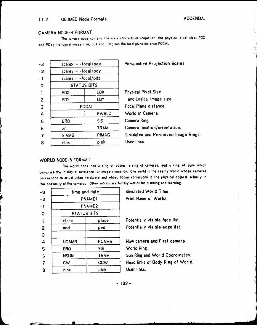
11.2 GEOMED Node Formats. ADDENDA.
CAMERA NODE-4 FORMAT Th« c»m«ri nod« contains th« sctl« conttjnts of projection, th« phytical piK«l tiz«, PDX
and POY; th« logical imae« siz«, LDX and LDY; and th« focal plan« dittanc« FOCAL
-J
-2
-1
0
1
2
3
4
5
6
7
8
scalex = -focal/pdx
scaley = -focal/pdy
scalez = -focal/pdz
STATUS BITS
PDX LDX
PDY LDY
FOCAL
PWRLD
BRO SIS
e.t TRAM
SIMAG PIMAG
nlnk pink
Perspective Projection Scales.
Physical Pixel Size
and Logical image size.
Focal Plane distance.
World of Camera.
Camera Ring.
Camera location/orientation.
Simulated and Perceived Image Rings.
User links.
WORLD NODE-5 FORMAT Th« world nod« hat a ring Of bodias, • ring of earner», and ■ ring of suns which
compnt« th« totality of «xisUnc« for imag« simulation On« world it th« reality world who«« cameras
corr«spond to actual vid«o hardwar« and whoes bodi«s correspond to th« physical objects actually in
th« proximity of th« cam«ras Other worlds ar« fantasy worlds for planning and Uarning.
Simulated World Time. -3
-2
-1
0
1
2
3
4
5
6
7
8
time and date
PNAME1
PNAME2
STATUS BITS
rfaca pface
ned ped
MCAMR PCAMR
BRO SIS
NSUN TRAM
CW CCW
nlnk pink
Print Name of World.
Potentially visible face list.
Potentially visible edge list.
Now camera and First camera.
World Ring.
Sun Ring and World Coordinates.
Head links of Body Ring of World.
User links.
133
J

11.2 GEOMED Node Formats. ADDENDA.
WINDOW NODE-6 FORMAT The displiy window node represents » mapping from a camera's image coordinates
(source image) to a display device's screen coordinates (object image) Window mappings can be
composed The mapped vurdow >s clipped to a border XL, XH, YL, YH in object coordinates after being
dilated by the scale tactor MAG The windows are organized into a ring of displays which each consists
of a ring of windows
-3
-2
1
0
1 2
3
5
6
7
8
sx SY
ox OY
MAG
STATUS BITS
XL XH
YL YH
NCAMR
BRO SIS
CW CCW
nlnk pink
Locus of center of Source Image.
Locus of center of Object Image.
Magnification of Window Mapping.
Object Image Clipping Border.
Now Camera of Window.
Window ring of a display.
Display ring of window rings.
User Links.
IMAGE NODE-7 FORMAT Image nodes represent either perceived contour images created by input from CRE or
simulated mosiac images created by tk,e I. Hden line eliminator, OCCULT Like a world, images carry a
list of bod1 s and a time reprpsennn* when Ih« image was taken Image nodes also carry a pointer to
a copy of the earner« and sun under which they were made
Corresponding Video image file name.
3 i
2 PNAME1
1 PNAME2
0 STATUS BITS
1
2
3
4 NCAMR PWRLD
5 NTIME PTIME
6 ALT
7 CW CCW
8 nlnk pink
Gamers Copy and World of this image,
image ring links to form a film.
Corresponding image.
Head links of image body ring.
User Links.
- 134
^^ta

11.2 GEOMED Node Formats. ADDENDA
BODY NODE-14 FORMAT Th« body node is the head of the iac«, edge and vertex rings which use word 1, 2, and
3 The body node carries a parts tree structure in word 4 and 5 There it • print name ot up to ten
characters carried in words -2 an -1 The links of the eighth word are always left free for linkage to
user data structures
-3
2
-1
0
1
2
3
4
5
6
7
8
PNAME1
PNAME2
STATUS BITS
NFACE PEACE
NED PED
NVT PVT
DAD SON
BRO SIS
alt TRAM
CW CCW
nlnk pink
Ten character print name.
Face ring.
Edge ring.
Vertex ring.
Parts Tree links: up and down tree.
Parts Tree links: ring of siblings.
Body coordinate system TRAM.
Body ring of world.
User links.
FACE NODE-15 FORMAT The face node carries a normalized face normal vector in AA, BB, and CC; the negative
distance of the face plane from the orgm, KK; photometric parameters are kept in words 4, 5 and 7
3 AA
2 BB
1 CC
0 STATUS BITS
1 NFACE PEACE
2 Ncnt PED
3 KK
4 red grn blu wht
5 Lr Lg Lb Lb Sm Sn
6 alt alt 2
7 QQ 3 nlnk pink
Face plane normal vector.
f'ace ring of a body.
Edge count and first edge.
Distance of face plane from origin.
Reflectivities under four filters.
Luminosities and Spectral constants.
Temporaries.
Video Intensity under four filters.
User Links.
135
.■^ ^^

11.2 GEOMEO Node Formats ADDENDA
EDGE NODE-16 FORMAT Th« imporUnt ti«ids ol th« wirjtd »of noo« ar» axplnnad in Ch«pt«r 2 Th« Mgativt
IhrM words if us«d (or «dg« co«)tici«nts ind (or clipped dupliy coordm«t«s o< th« «dg« Th« ill,
■H2 and cw fi.id «r« used is («mponry (i«lds in OCCULT. BIN and »0 on Th« CCW dald points it
body of »de* «nd •xp.dites BGET Th« nlnK wid plnK dalds art Ktpt «mpfy for developmental work
Clipped Display Coordinates or
2-D Edge Coefficients or
3-D line Cosines.
-3
2
-1
0
1
2
3
5
6
7
8
xldc AA yldc
x2dc BB y2dc
CC
STATUS BITS
NFACE PEACE
NED PED
NVT PVT
NCW PCW
NCCW PCCW
alt alt2
cw ccw
nlnk pin*
Two faces of the edge
Edge ring of the body.
Two vertices of the edge.
Wings: neighboring edges in PEACE and
Neighboring edges in NEACE.
Temporaries.
Temporary and Body Link.
User links.
VERTEX NODE-17 FORMAT The vertex node carries a point's locus in three coordinate systems: world coordinates,
perspective proofed coordinates and display coordinates The first edge of a vertex perimeter it
contained in the PED field The alt, alt2. cw, ccw and Tjomt (ields art ustd as temporaries
■3
-2
-1
0
I
2
3
4
5
6
7
8
XWC
YWC
ZWC
STATUS BITS
XDC YDC
Tjoint PED
NVT PVT
XPP
YPP
alt ZPP alt 2
cw ccw
nlnk pink
World Locus
Display Screen Locus.
Temporary and First Edge.
Vertex ring of the body.
Perspective Projected Locus.
...also used for temporaries.
temporaries.
User links.
- 136
mtm J