ada: an r package for stochastic boosting · the underlying engine is the rpart ... an r package...

JSS Journal of Statistical SoftwareOctober 2006, Volume 17, Issue 2. http://www.jstatsoft.org/

ada: An R Package for Stochastic Boosting

Mark CulpUniversity of Michigan

Kjell JohnsonPfizer Global Research

and Development

George MichailidisUniversity of Michigan

Abstract

Boosting is an iterative algorithm that combines simple classification rules with ‘mediocre’performance in terms of misclassification error rate to produce a highly accurate classifi-cation rule. Stochastic gradient boosting provides an enhancement which incorporates arandom mechanism at each boosting step showing an improvement in performance andspeed in generating the ensemble. ada is an R package that implements three popularvariants of boosting, together with a version of stochastic gradient boosting. In addi-tion, useful plots for data analytic purposes are provided along with an extension to themulti-class case. The algorithms are illustrated with synthetic and real data sets.

Keywords: boosting algorithms, R, machine learning, classification, implementation of statis-tical algorithms.

1. Introduction

Boosting has proved to be an effective method to improve the performance of base classifiers,both theoretically and empirically. The underlying idea is to combine simple classificationrules (the base classifiers) to form an ensemble, whose performance is significantly improved.The origins of boosting lie in PAC learning theory (Valiant 1984), which established thatlearners that exhibit a performance slightly better than random guessing when appropriatelycombined can perform very well.

A provably polynomial complexity boosting algorithm was derived in (Schapire 1990), whereasthe Adaptive Boosting (AdaBoost) algorithm in various varieties (Freund and Schapire 1996,1997) proved to be a practical implementation of the boosting ensemble method. Since itsintroduction, many authors have sought to explain and improve upon the AdaBoost algorithm.In (Friedman, Hastie, and Tibshirani 2000), it was shown that the AdaBoost algorithm canbe thought of as a stage-wise gradient descent procedure that minimizes an exponential lossfunction. In addition, three modifications of the original algorithm were proposed: Gentle-,

http://www.jstatsoft.org/

2 ada: An R Package for Stochastic Boosting

Logit-, and Real AdaBoost.

Recently, several authors have explored regularizing the boosting algorithm (Friedman 2001;Rosset, Zhu, and Hastie 2004). For example, if classification trees constitute the base clas-sifiers, regularization is accomplished through the learning rate parameter. This parametercontrols the algorithm’s ability to search the collection of all possible trees for the given dataset. However, the improved performance in terms of predictive accuracy comes at a heavycomputational cost. Stochastic gradient boosting (Friedman 2002; Ridgeway 2006) utilizesa random mechanism for regularization purposes and achieves significant computational sav-ings.

The ada package implements the original AdaBoost algorithm, along with the Gentle andReal AdaBoost variants, using both exponential and logistic loss functions for classificationproblems. In addition, it allows the user to implement regularized versions of these methodsby using the learning rate as a tuning parameter, which lead to improved computationalperformance. The base classifiers employed are classification/regression trees and thereforethe underlying engine is the rpart package. The ada package uses rpart’s functionality forhandling missing data and surrogate splits (Therneau and Atkinson 2005). Some importantfeatures incorporated in the ada package are: (i) the use of both regression and classificationtrees for boosting, (ii) various useful plots that aid in assessing variable importance andrelationships between subsets of variables and (iii) tweaking the controls of the rpart functionto become applicable for boosting purposes.

The boosting framework typically accomplishes the difficult task of providing both strongpredictive performance and useful model diagnostics, which has made it desirable for manyclassification problems (Freund and Schapire 1996, 1997; Hastie, Tibshirani, and Friedman2001). In this paper, we provide analysis of boosting on pharmacology data (Sugata and Abe2001), where the goal is to predict whether a compound is soluble, and to identify variablesthat are important for predicting this property. In addition to pharmacology, boosting al-gorithms have encompassed a wide range of applications including tumor identification andgene expression data (Dettling 2004), proteomics data (Ulintz, Zhu, Qin, and Andrews 2006),financial and marketing data (Boonyanunta and Zeephongsekul 2003; Lemmens and Croux2005), fisheries data (Kawakita, Minami, Eguchi, and Lennert-Cody 2005), and microscopeimaging data (Huang and Murphy 2004). For many of these applications, ada will be par-ticularly useful since it implements well documented tools for assessing variable importance,evaluating training and testing error rates, and viewing pairwise plots of the data.

Currently, free R (R Development Core Team 2006) packages exist for boosting that efficientlybuild regression trees, smoothing splines, and additive models such as gbm (Ridgeway 2006)and mboost (Hothorn and Buhlmann 2006a,b). The gbm package offers two versions ofboosting for classification (gentle boost under logistic and exponential loss). In addition, itincludes squared error, absolute error, Poisson and Cox type loss functions. However, thelatter loss functions are not natural or recommended for classification purposes (Hastie et al.2001). The mboost package has to a large extent similar functionality as the gbm packageand in addition implements the general gradient boosting framework using regression-basedlearners. In our experience, these packages are more suited for users in need of using boostingin models with a continuous or count type outcome. On the other hand, the ada packageprovides a straightforward, well-documented, and broad boosting routine for classification,ideally suited for small to moderate-sized data sets. As an enhancement over current boostingpackages, ada incorporates two popular loss functions for three boosting variants, variance

Journal of Statistical Software 3

reduction components (similar to bagging), regularization, and performance diagnostics. Inaddition, at each iteration ada incorporates cross-validation to determine tree depth, whichresolves the selection of tree depth associated with gbm. ada’s extensive documentationand ease of use, provides a natural package for individuals interested in quickly familiarizingthemselves with the boosting methodology and assessing how boosting would perform on theirdata. The ada package is freely available from http://CRAN.R-project.org/.The paper is organized as follows: in section 2 a brief introduction to the various boostingalgorithms implemented in ada is provided; section 3 discusses various implementation issues,while in section 4 a description of the available functions is given. Finally, section 5 discussesseveral practical issues in the context of real data examples.

2. A brief account of boosting algorithms

In this section a brief synopsis of the history of AdaBoost (now referred to as DiscreteAdaBoost) is given, which discusses the origins of this algorithm, as well as the relationshipbetween boosting and additive models. The next section focuses on implementation detailsfor each boosting variant implemented in the package. This is accomplished by presented ageneral boosting algorithm and then discussing the various variants as special cases.In a classification problem, a training data set consisting of n objects is available. Eachobject is characterized by a p-dimensional attribute (feature/variable) vector x, belonging toa suitable space (e.g. Rp), and a class label (response) y ∈ {+1,−1}. The objective is toconstruct a decision (classification) rule F (x) that would accurately predict the class labelsof objects for which only the attribute vector is observed.

2.1. Historical perspective

In 1996, Freund and Schapire (Freund and Schapire 1996) produced the well-knownAdaBoost.M1 (also known as Discrete AdaBoost) algorithm (given below). In short,AdaBoost.M1 generates a sequentially weighted set of weak base classifiers that are com-bined to form an overall strong classifier. In each step of the sequence, AdaBoost attemptsto find an optimal classifier according to the current distribution of weights on the observa-tions. If an observation is incorrectly classified using the current distribution of weights, thenthe observation will receive more weight in the next iteration. On the other hand, correctlyclassified observations under the current distribution of weights will receive less weight inthe next iteration. In the final overall model, classifiers that are accurate predictors of thetraining data receive more weight, whereas, classifiers that are poor predictors receive lessweight. Thus, AdaBoost uses a sequence of simple weighted classifiers, each forced to learna different aspect of the data, to generate a final, comprehensive classifier, which with highprobability outperforms in terms of misclassification error rate any individual classifier. Thebasic steps of the algorithm as described next (Algorithm 1):In 2000, Friedman et al. (2000) established connections of the AdaBoost.M1 algorithm tostatistical concepts such as loss functions, additive modeling, and logistic regression. Inparticular, they showed that AdaBoost.M1 fits a forward stagewise additive logistic regressionmodel that minimizes the expectation of the exponential loss function, e−yF (x) , with F (x)denoting the boosted classifier.While the AdaBoost algorithm has been shown empirically to improve classification accuracy,

http://CRAN.R-project.org/


Algorithm 1 AdaBoost1: Initialize weights wi = 1

n2: for m = 1 to M do3: fit y = hm(x) as the base weighted classifier using wi and d

4: let W−(hm) =∑N

i=1 wiI{yihm(xi) = −1} and αm = log(

1−W−(h)W−(h)

)5: wi = wi exp{αmI{yi 6= hm(xi)}} scaled to sum to one ∀i ∈ {1, . . . , N}6: end for

it produces at each stage as output the object’s predicted label. This coarse information mayhinder the efficiency of the algorithm in finding an optimal classification model. To overcomethis deficiency, several proposals have been put forth in the literature; for example, the al-gorithm outputs a real-valued prediction rather than class labels at each stage of boosting.The latter variant of boosting corresponds to the Real AdaBoost algorithm, where the classprobability estimate is converted using the half-log ratio to a real valued scale. This value isthen used to represent an observation’s contribution to the final overall model. Furthermore,observation weights for subsequent iterations are updated according to the exponential lossfunction of AdaBoost. Like Discrete AdaBoost, the Real AdaBoost algorithm attempts tominimize the expectation of e−yF (x). In general, these modifications allow Real AdaBoost tomore efficiently find an optimal classification model relative to AdaBoost.M1. In addition tothe Real AdaBoost modification, Friedman et al. (Friedman et al. 2000) proposed a furtherextension called the Gentle AdaBoost algorithm which minimizes the exponential loss func-tion of AdaBoost through a sequence of Newton steps. Although Real AdaBoost and GentleAdaBoost optimize the same loss function and perform similarly on identical data sets, GentleAdaBoost is numerically superior because it does not rely on the half-log ratio.

2.2. Stochastic boosting

Boosting inherently relies on a gradient descent search for optimizing the underlying lossfunction to determine both the weights and the learner at each iteration (Friedman 2001). InStochastic Gradient Boosting (SGB) a random permutation sampling strategy is employedat each iteration to obtain a refined training set. The full SGB algorithm with the gradientboosting modification relies on the regularization parameter ν ∈ [0, 1], the so-called learningrate.

Algorithm 2 Stochastic Gradient Boosting Algorithm1: Initialize F (x) := 02: for m = 1 to M do3: Set wi = − δL(y,g)

δg |g=F (x)

4: Fit y = η(hm(x)) as the base weighted classifier using | wi |, with training sample πm

5: Compute line search step αm = arg minα∑

i∈πmL(yi, F (x) + αη(hm(xi)))

(in some cases this step may be omitted or αm = 1)6: Update F (x) = F (x) + ναmη(hm(x))7: end for

The algorithm in its general form can operate under an arbitrary loss function; ada implementsboth the exponential (L(y, f) = e−yf ) and logistic (L(y, f) = log(1+e−yf )) loss functions. The


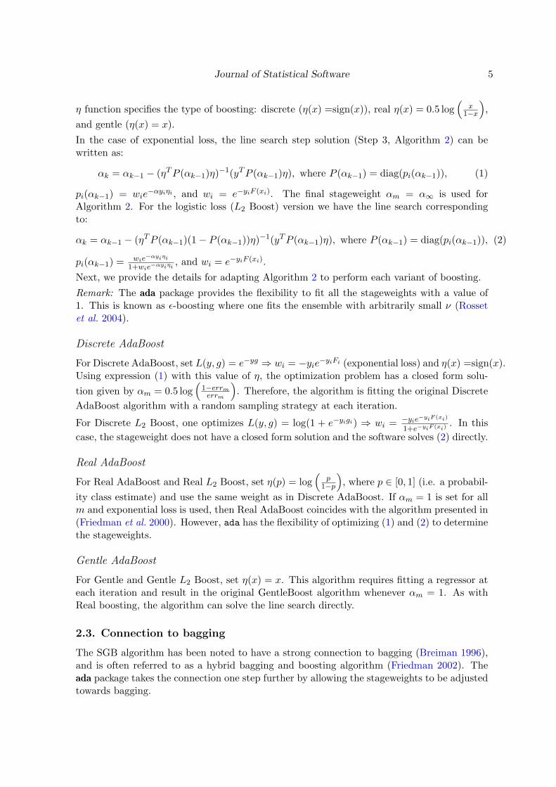
η function specifies the type of boosting: discrete (η(x) =sign(x)), real η(x) = 0.5 log(

x1−x

),

and gentle (η(x) = x).

In the case of exponential loss, the line search step solution (Step 3, Algorithm 2) can bewritten as:

αk = αk−1 − (ηT P (αk−1)η)−1(yT P (αk−1)η), where P (αk−1) = diag(pi(αk−1)), (1)

pi(αk−1) = wie−αyiηi , and wi = e−yiF (xi). The final stageweight αm = α∞ is used for

Algorithm 2. For the logistic loss (L2 Boost) version we have the line search correspondingto:

αk = αk−1 − (ηT P (αk−1)(1− P (αk−1))η)−1(yT P (αk−1)η), where P (αk−1) = diag(pi(αk−1)), (2)

pi(αk−1) = wie−αyiηi

1+wie−αyiηi, and wi = e−yiF (xi).

Next, we provide the details for adapting Algorithm 2 to perform each variant of boosting.

Remark: The ada package provides the flexibility to fit all the stageweights with a value of1. This is known as ε-boosting where one fits the ensemble with arbitrarily small ν (Rossetet al. 2004).

Discrete AdaBoost

For Discrete AdaBoost, set L(y, g) = e−yg ⇒ wi = −yie−yiFi (exponential loss) and η(x) =sign(x).

Using expression (1) with this value of η, the optimization problem has a closed form solu-tion given by αm = 0.5 log

(1−errm

errm

). Therefore, the algorithm is fitting the original Discrete

AdaBoost algorithm with a random sampling strategy at each iteration.

For Discrete L2 Boost, one optimizes L(y, g) = log(1 + e−yigi) ⇒ wi = −yie−yiF (xi)

1+e−yiF (xi). In this

case, the stageweight does not have a closed form solution and the software solves (2) directly.

Real AdaBoost

For Real AdaBoost and Real L2 Boost, set η(p) = log(

p1−p

), where p ∈ [0, 1] (i.e. a probabil-

ity class estimate) and use the same weight as in Discrete AdaBoost. If αm = 1 is set for allm and exponential loss is used, then Real AdaBoost coincides with the algorithm presented in(Friedman et al. 2000). However, ada has the flexibility of optimizing (1) and (2) to determinethe stageweights.

Gentle AdaBoost

For Gentle and Gentle L2 Boost, set η(x) = x. This algorithm requires fitting a regressor ateach iteration and result in the original GentleBoost algorithm whenever αm = 1. As withReal boosting, the algorithm can solve the line search directly.

2.3. Connection to bagging

The SGB algorithm has been noted to have a strong connection to bagging (Breiman 1996),and is often referred to as a hybrid bagging and boosting algorithm (Friedman 2002). Theada package takes the connection one step further by allowing the stageweights to be adjustedtowards bagging.


A close inspection reveals that if one executes Algorithm 2 with ν := 0, then the ensembleof trees will be generated by random subsamples of the data with identical case weights(i.e. letting Fν(x) be the ada output, then F0(x) = 0 ∗

∑Mm=1 αmhm(x)). This is the exact

tree fitting process used to bag trees (Breiman 1996), with the exception that in baggingthe ensemble results as an average of the trees (i.e. B(x) = 1

M

∑Mm=1 hm(x) is a bagged

ensemble but under the same random settings one would obtain the same trees as withF0(x)). In light of this, we add a shift=TRUE argument which supplies a post processingshift of the ensemble towards bagging after constructing the ensemble (i.e. the final ensembleis Fν(x) = (1 − ν)B(x) + Fν(x), where F0(x) = B(x) equates to bagging). However, unlikebagging (with the exception of ν = 0) the individual h’s are obtained via a greedy weightingprocess. In the case of ε-boosting (i.e. αm := 1) then the resulting ensemble is an averageover h.

3. Implementation issues

In this section we discuss implementation issues for the ada package.

3.1. Functional structure

The functional layout for the ada package is shown in Figure 1. An object of class ada can

Figure 1: The functional flow of ada. The top section consists of the functions used to createthe ada object, while the bottom section are the functions invoked using an initialized adaobject. The yellow functions are called only by ada, the red functions are called by the userand the green functions are called by both.


be created by invoking the functions ada, which calls either ada.formula or ada.default,depending on the input to ada. The ada.formula function is a generic formula wrapper forada.default that allows the flexibility of a formula object as input. The ada.default func-tion, in turn, calls the four functions that correspond to the boosting algorithms: discrete.ada,real.ada, logit.ada and gentle.ada. Once an object of class ada is created, the user caninvoke the standard R commands: predict, summary, print, pairs, update, or plot. Inaddition, ada includes a varplot and addtest function, which we discuss below.

3.2. Construction of base learners using rpart

The most popular base (weak) learners employed by both boosting and stochastic boostingalgorithms are classification or regression trees. Both of these algorithms are implemented inthe rpart package, and can be tweaked for either boosting or stochastic gradient boosting.Because the ada package uses rpart as its engine, ada inherits the flexibility and advantagesof rpart (Therneau and Atkinson 2005). Because of rpart, ada can handle missing data, canimplement either classification or regression trees, and can use cross-validation to automat-ically determine individual tree depth. In addition, because ada uses rpart, ada will inheritany improvements made to rpart.Remark: Notice, that the gbm package, for instance, uses its own internal recursive partitionerfor only computing regression trees with no means for estimating tree depth. However, wefeel that the flexibility and enhancements provided by rpart yields a worthwhile tree enginefor ada.

Setting rpart.control

The rpart function selects tree depth by using an internal complexity measure together withcross-validation. In the case of SGB we have empirically noticed strong performance withthis automatic choice of tree depth (especially for larger data sets).However, in deterministic gradient boosting, the tree size is usually selected a priori. Forexample, stumps (2-split) or 4-split trees (e.g. split the data into a maximum of 4 groups)are commonly selected as the weak learners. In rpart one should set cp=-1, which forces thetree to split until the depth of the tree achieves the maxdepth setting. Thus, by specifyingthe maxdepth argument, the number of splits can be controlled. It is important to note thatthe maxdepth argument works on a log2 scale, hence the number of splits is a power of 2.In small data sets, it is useful to appropriately specify the minsplit argument, in order toensure that at least one split will be obtained. Finally, it is worth noting that a theoreticallyrigorous approach for setting the tree depth in any form of boosting is still an open problem(Segal 2004).The following code illustrates how the control parameters for generating stumps and 4-splittrees:

> library("ada")

Loading required package: rpart

> default <- rpart.control()

> stump <- rpart.control(cp = -1 , maxdepth = 1 , minsplit = 0)

> four <- rpart.control(cp = -1 , maxdepth = 2 , minsplit = 0)


4. Description of the functions available in the ada package

To illustrate the functions available in ada, we use a ten dimensional synthetic data set,comprised of two interspersed classes exhibiting a sinusoid pattern (Figure 2). In this data,two variables that determine the class shapes were corrupted by eight dimensions of standardGaussian noise, creating a difficult to trace boundary between the classes. Five hundredobservations equally divided among the two classes were generated, and 20% were assignedto the training set. The following R code was used to generate the data.

> n <- 500

> p <- 10

> f <- function(x, a, b, d) a * (x - b)^2 + d

> set.seed(100)

> x1 <- runif(n/2, 0, 4)

> y1 <- f(x1, -1, 2, 1.7)+runif(n/2, -1, 1)

> x2 <- runif(n/2, 2, 6)

> y2 <- f(x2, 1, 4, -1.7)+runif(n/2, -1, 1)

> y <- c(rep(1, n/2), rep(2, n/2))

> mat <- matrix(rnorm(n * 8), ncol = 8)

> dat <- data.frame(y = y, x1 = c(x1, x2), x2 = c(y1, y2), mat)

> names(dat) <- c("y", paste("x", 1:10, sep = ""))

> plot(dat$x1, dat$x2, pch = c(1:2)[y], col = c(1, 8)[y],

+ xlab=names(dat)[2], ylab=names(dat)[3])

> indtrain <- sample(1:n, 100, FALSE)

●

●

●

●

●●

●

●

●

●

●

●●

●

●

●

●

●

●●●

●●

●

●

● ●

●

●

●

●

●

●

●

●

●

●

●

●

●

●

●

●●

●

● ●

●

●

●

●

●

●

●

●●

●

●

●

●●

●

●

●

●●

●

●

●

●

●●

●

●

●

●

●

●

●●

●

●

●

●

●

●

●

●

●

●

●

●

●

●

●

●

●

●

●

●

●

●

●

●

●

●

●

●

●

●

●

●

●

●

●

●●

●● ●

●

● ●

●●

●

●

●

●

●

●

●

●

●

●

●

●

●

●

●

●

●

●

●

●

●

●●

●

●

●

●

●

●

●

●●

●

●

●

●

●

●

●

●

●

●

●

●

●

●

●

●

●

●

●

●

●

●

●

●

●

●

●

●

●

●●

●

●

●

●

●

●

●

●

●

●

●●

●

●

●

●●

●

●

●

●

●

●●

●

●

●

●

●

●

●

●

●

●●

●

●

●

●

●

●

● ●

●

●●●

●

●

●

●

●

●

●

●

●

●

●●

●

●

●

0 1 2 3 4 5 6

−3

−2

−1

01

23

x1

x2

Figure 2: Plot of the two informative variables, colored by the response.


> train <- dat[indtrain,]

> test <- dat[-indtrain,]

4.1. Creating an ada object

Objects of class ada are created by a call to the appropriate function, specifying the type ofboosting (Discrete, Real, etc).

Discrete AdaBoost

To model the synthetic data sets with discrete AdaBoost under exponential loss (using stumpswith 50 iterations) call:

> default <- rpart.control()

> gdis <- ada(y~., data = train, iter = 50, loss = "e", type = "discrete",

+ control = default)

> gdis

Call: ada(y ~ ., data = train, iter = 50, loss = "e", type ="discrete", control=default)

Loss: exponential Method: discrete Iteration: 50

Final Confusion Matrix for Data:Final Prediction

True value 1 21 49 32 8 40

Train Error: 0.11

Out-Of-Bag Error: 0.14 iteration= 9

Additional Estimates of number of iterations:

train.err1 train.kap147 50

Notice that the output gives the training error, confusion matrix and three estimates of thenumber of iterations. In this example, one could use the Out-Of-Bag (OOB) estimate for 9iterations, training error estimate of 47, or the kappa error estimate of 50 iterations.

To add the testing data set to the model, simply use the addtest function. This functionallows us to evaluate the testing set without refitting the model.

> gdis <- addtest(gdis, test[,-1], test[,1]))

> gdis


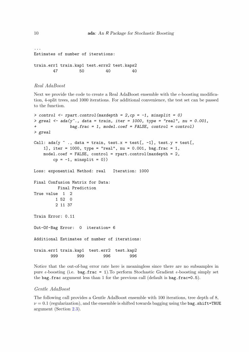
...Estimates of number of iterations:

train.err1 train.kap1 test.errs2 test.kaps247 50 40 40

Real AdaBoost

Next we provide the code to create a Real AdaBoost ensemble with the ε-boosting modifica-tion, 4-split trees, and 1000 iterations. For additional convenience, the test set can be passedto the function.

> control <- rpart.control(maxdepth = 2,cp = -1, minsplit = 0)

> greal <- ada(y~., data = train, iter = 1000, type = "real", nu = 0.001,

+ bag.frac = 1, model.coef = FALSE, control = control)

> greal

Call: ada(y ~ ., data = train, test.x = test[, -1], test.y = test[,1], iter = 1000, type = "real", nu = 0.001, bag.frac = 1,model.coef = FALSE, control = rpart.control(maxdepth = 2,

cp = -1, minsplit = 0))

Loss: exponential Method: real Iteration: 1000


True value 1 21 52 02 11 37

Train Error: 0.11

Out-Of-Bag Error: 0 iteration= 6


train.err1 train.kap1 test.err2 test.kap2999 999 996 996

Notice that the out-of-bag error rate here is meaningless since there are no subsamples inpure ε-boosting (i.e. bag.frac = 1).To perform Stochastic Gradient ε-boosting simply setthe bag.frac argument less than 1 for the previous call (default is bag.frac=0.5).

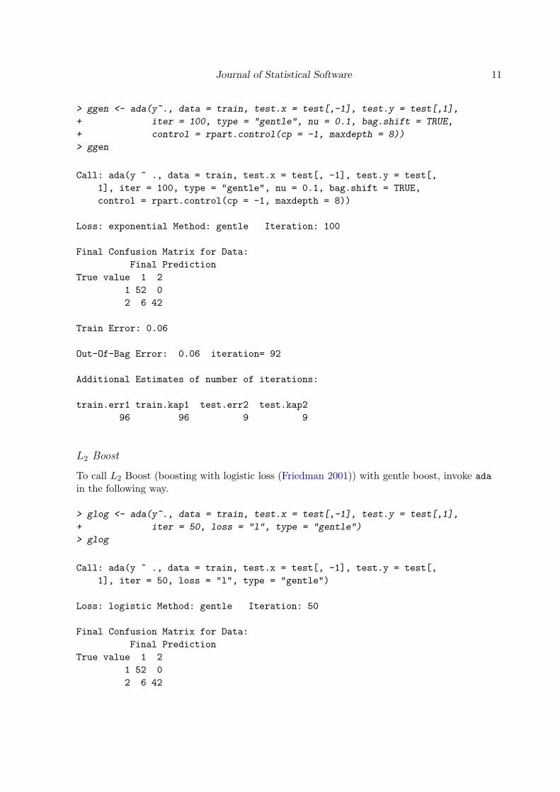
Gentle AdaBoost

The following call provides a Gentle AdaBoost ensemble with 100 iterations, tree depth of 8,ν = 0.1 (regularization), and the ensemble is shifted towards bagging using the bag.shift=TRUEargument (Section 2.3).


> ggen <- ada(y~., data = train, test.x = test[,-1], test.y = test[,1],

+ iter = 100, type = "gentle", nu = 0.1, bag.shift = TRUE,

+ control = rpart.control(cp = -1, maxdepth = 8))

> ggen

Call: ada(y ~ ., data = train, test.x = test[, -1], test.y = test[,1], iter = 100, type = "gentle", nu = 0.1, bag.shift = TRUE,control = rpart.control(cp = -1, maxdepth = 8))

Loss: exponential Method: gentle Iteration: 100


True value 1 21 52 02 6 42

Train Error: 0.06

Out-Of-Bag Error: 0.06 iteration= 92



L2 Boost

To call L2 Boost (boosting with logistic loss (Friedman 2001)) with gentle boost, invoke adain the following way.

> glog <- ada(y~., data = train, test.x = test[,-1], test.y = test[,1],

+ iter = 50, loss = "l", type = "gentle")

> glog

Call: ada(y ~ ., data = train, test.x = test[, -1], test.y = test[,1], iter = 50, loss = "l", type = "gentle")

Loss: logistic Method: gentle Iteration: 50


True value 1 21 52 02 6 42


Train Error: 0.06

ut-Of-Bag Error: 0.1 iteration= 50



In addition to performing gentle boost the logistic loss function can be invoked with thetype="discrete" or type="real".

Stageweight convergence

For many of these methods a Newton Step is necessary for the convergence of the stageweightat each iteration. To see the convergence use the verbose=TRUE flag:

> greal <- ada(y~., data = train, test.x = test[,-1], test.y = test[,1],

+ iter = 50, type = "real", verbose = TRUE)

FINAL: iter= 4 rate= 9.240109e-19...FINAL: iter= 3 rate= 5.890882e-15

For this example the stageweights converged quickly. In some situations the convergence maynot be as fast; to increase the number of iterations for convergence purposes use the max.iterargument.

4.2. Using an ada object

Upon building an ada object, one can explore the model performance and characteristicsthrough several different tools.

The plot function

The ada plot function overrides the generic plot function in R by plotting the trainingerror versus iteration number for a given boosting ensemble. If the testing data sets havebeen passed into the ada object then the testing errors can easily be plotted by using thetest=TRUE argument.

The following call shows how to create a plot using discrete adaboost on the training data(Figure 3 (right)).

> plot(gdis)

Notice that the training error steadily decreases across iterations. This shows that boostingcan effectively learn the features in a data set. However, a more valuable diagnostic plot wouldinvolve the corresponding test set error plot. The following call creates both the training andtesting error plots side-by-side, as seen in Figure 3 (right).


0 10 20 30 40 50

0.12

0.14

0.16

0.18

0.20

0.22

0.24

Iteration 1 to 50

Err

or

50

11

11

1

Training Error

1 Train

0 10 20 30 40 50

0.10

0.15

0.20

0.25

0.30

0.35

Iteration 1 to 50

Err

or50

1 11 1

1

Training And Testing Error

2 2 2 2 2

12

TrainTest1

Figure 3: Training error by iteration number for the example data (right). The training andtesting error by iteration number for the example data (left).

> plot(gdis, FALSE, TRUE)

Remark: In many situations the class priors (proportion of true responses) are unbalanced;in these situations, learning algorithms often focus on learning the larger set. Hence, errorstend to appear low, but only because the algorithm classifies objects into the larger class. Analternative measure to absolute classification error is the Kappa statistic (Cohen 1960), whichadjusts for class imbalances.

The summary function

Another utility often used with objects in R is summary. To summarize an ada object thesummary function returns the kappa value and training accuracy for the final iteration in agiven ensemble. If testing data sets are included, then the accuracy and kappa value willalso be reported. The argument n.iter allows the user to specify which iteration to report(default is the model iter specification). The following code shows how to call this functionusing Gentle AdaBoost with the OOB error minimum.

> summary(ggen, n.iter = 64)

Call: ada(y ~ ., data = train, test.x = test[, -1], test.y = test[,1], iter = 100, type = "gentle", nu = 0.1, bag.shift = TRUE,control = rpart.control(cp = -1, maxdepth = 8))


Training Results


Accuracy: 0.96 Kappa: 0.92

Testing Results


The predict function

The predict function is written to match the arguments of the predict.rpart generic func-tion. Hence, the arguments consist of object, newdata, and type, which give a specificprediction result. The default type for this function is to return the predicted vector of classlabels for the training data. The options type="prob", type="both" and type="F" eithergive the probability class estimates, both the portability class estimates and the vector oflabels, or the weighted sum over the ensemble, respectively. The following code shows how topredict with Real AdaBoost.

> pred <- predict(greal, train[,-1])

> table(pred)

1 256 44

To get the probability class estimates for the training data input:

> pred <- predict(greal, train[,-1], type = "prob")

> pred

[,1] [,2]451 0.317362113 0.68263788786 0.851147564 0.148852436

...257 0.007765103 0.99223489774 0.851265307 0.148734693

The first column provides the number of the actual observation in the original data set.

Remark: The probability class estimate for any boosting algorithm is defined as P (Y = 1 |x) = e2F (x)

1+e2F (x) . However, since the function ex is considered infinite by R for large x it isnecessary to compute this value on the logarithmic scale and force it to 1 if e2F (x) = ∞. Asa result, one can not get the original F from this transformation, which is needed for themulti-class case. This is the rationale for having the option of setting type="F". The usageof this argument setting is shown in the multi-class example in the next section.

Remark: The newdata option requires a data.frame of observations with the exact samevariable names as the training data. If a matrix format is used to represent the training data,then the variable names will most likely be the default V1, . . . , Vp. The following code showshow to change the names of the columns, if the training data are in a matrix or a data.frameformat, respectively.


> test <- as.data.frame(test)

> names(test) <- c("y", paste("V", 1:p, sep=""))

> names(test) <- names(train)

The update function

Invoke the following command to add more trees to the glog ensemble, which was constructedabove with 20 trees.

> glog <- update(glog, train[,-1], train[,1], test[,-1], test[,1], n.iter = 50)

> glog

Loss: logistic Method: gentle Iteration: 100...train.err1 train.kap1 test.err2 test.kap2

75 75 96 96

The varplot function

Gentle AdaBoost will be used to illustrate the variable importance function. The followingcode shows how to plot the variables ordered by the importance score defined in (Hastie et al.2001).

> varplot(ggen)

Figure 4 gives us the scores for the variable assessment for Gentle AdaBoost.

To obtain the variable scores directly (without a plot) use the following code.

> vip <- varplot(gdis, plot.it = FALSE, type = "scores")

> round(vip, 4)

x1 x6 x5 x10 x2 x4 x9 x3 x8 x70.0070 0.0036 0.0035 0.0034 0.0028 0.0027 0.0025 0.0024 0.0023 0.0017

The pairs function

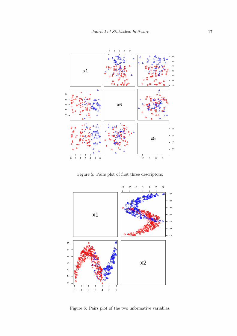
The pairs tool produces a visualization of the pairwise relationships between a subset ofvariables in the data set. The upper panel plots represent the true class labels as colors foreach pairwise relationship, while the lower panel gives the predicted class for each observation.Also the observations in the plots on the lower panel are scaled by the class probabilityestimate, where the size of the point represents the probability estimate. Hence this plot canhelp identify observations that are difficult for boosting to classify.

To generate the pairwise plots for the three top variables determined by the varplot function,issue the command:

> pairs(gdis, train[,-1], maxvar = 3)


x9

x3

x8

x7

x6

x10

x2

x4

x5

x1

●

●

●

●

●

●

●

●

●

●

0.014 0.016 0.018 0.020 0.022 0.024 0.026

Variable Importance Plot

Score

Figure 4: Variable importance scores produced by the varplot command.

Pairs can also be used to explore the relationships among variables in the test set. If theresponse for the test set is unknown, the observations will be plotted in black.

> pairs(gdis, train[,-1], var = 1:2,test.x = test[,-1],

+ test.y = test[,1],test.only = TRUE)

As a final note, to view both the testing and training data on the same plot, leave test.onlyas FALSE and issue the above command with either var=· · · for a specific set of variables ormaxvar=k for the top k variables.

5. Examples

The examples below will illustrate various aspects and uses of the ada package.

5.1. Diagnostics and model selection

To illustrate ada and validate its performance, we will use an example from Hastie et al.(2001), pp. 300-308. A ten dimensional data set comprised of 12,000 observations wasgenerated, where each variable is an independent and identically distributed mean zero,variance one, normal variate. The response was computed using each variable equally as,Y = 2× 1{P

X2j >χ2

10(0.5)=9.34} − 1, using the following code.


x1

−2 −1 0 1 2

●

●

●

●

●

●

●

●

●

●●

●

●

● ●

●●

●

●

●

●●

●

●

●

●

●●

●

●●

●

●●

●

●●

●

●

●

●

●

●●●

● ●

●

●

●

●

●

01

23

45

6

●

●

●

●

●

●

●

●

●

●●

●

●

● ●

●●

●

●

●

●●

●

●

●

●

●●●

●●

●

●●

●

●●

●

●

●

●

●

●●●

● ●

●

●

●

●

●−

2−

10

12

●

●

●

●●

●●

●

●

●

●

●

●

●

●

●

●

●

●

● ●

●

●

●

●

●

●

●

●

●

●

●

●

●

●

●

●

●

●

●

●

●

●

●

●

●

●

●

●

●

●

●

●

●

●●

●

x6●

●

●●

●●

●●

●

●●

●

●

●

●

●

●●

●

●

● ●

●

●

●

●

●

●

●

●

●

●

●

●

●

●

●

●

●

●

●

●

●

●

●

●

●

●

●

●●

●

0 1 2 3 4 5 6

●

●

●

●

●

●

●

●

●

●●

●

●

●

●●

●

● ●

●

●

●

●

●

●

●

●

●

● ●

●●

●

●

●●

●

●

●

●

●

●

●

●

●

●

●

●

●

●

●

●

●

●

●

●

●

●

●

●

●

●

●

●

●

●

●●

●

●

●

●●

●

●●

●

●

●

●

●

●

●

●

●

● ●

●●

●

●

●●

●

●

●

●

●

●

●

●

●

●

●

●

●

●

●

●

●

●

●

●

●

−2 −1 0 1

−2

−1

01

x5

Figure 5: Pairs plot of first three descriptors.

x1

−3 −2 −1 0 1 2 3

01

23

45

6

●●

●

●

●

●

●

●

●

●

●

●

●

●

● ●

●

●

●●

●

●

●

●

●

●

●

●

●

●

●

●

●●

●

●●

●

●

●

●

●

●●

● ●

●

●

●

●

●

●

●

●

●

●

●

●

●

●

●

●●

●

●●

●

●

●

●●

●

●

●

●

●●

●

●

●

●●●

●

●

●

●

●

●

●

●

●

●

●●

●

●

●

●

●

●

●

●

● ●

●●

●

●

●

●

● ●

●●

●

●

● ●

●

●

●

●

●

●●

●

●●

●

●●

●

●●

●

●

●

●

●

●

●

●

●

●

●●

●

●

●

●

●

●

●

●

●

●

●

●●

●

●

●

●

●

●

●●

●

●

●

●

●

●

●

●

●

●

●●

●

●

●

●

●

●

●

●

●

●●

●

●

●●

● ●

●

0 1 2 3 4 5 6

−3

−2

−1

01

23

●

●●

●

●

●

●

●

●

●●

●

●

●

●●●

●

●

●

●

●

●

●

●

●

●

●

●●

●

●

●

●

●

●

●

●

●

●

●

●

●

●

●

●

●●●

●

●

●●

●

●

●

●

●

●

●

●

●

●

●

●

●

●

●

●

●

●

●

●

●●

●

●

●

●

●

●

●

● ●

●

● ●

●

●

●●

●

●

●

●

●

●●

●

●

●

●

●

●

●

●

●

●

●

●

●

●

●

●

●

●

●

●

●

●

●

●

●

●

●

●

●

●

●

●

●

●

●●

●

●

●

●

●

●

●

●

●

●

●

●

●●

●●

●

●

●

●

●

●●

●

●

●

●

●

●

●

●●

●●

●

●

●

●

●

●

●

●

●

●

●

●

●

●

●

●

●

●

●

●

●

●

● ●

●

●

●

●

●

●

●

●

●

●●

●

●

●

●

●

●

●

●

●

●

●

●●

●●

●

●●

●●

●

●

●

●

●

●

●

●

●

●

●

●

●

●

●

●

●

●

●

●

●

●

●

●

●

●

●

●

●

●

●●

●

●

●

x2

Figure 6: Pairs plot of the two informative variables.


> n <- 12000

> p <- 10

> set.seed(100)

> x <- matrix(rnorm(n*p), ncol=p)

> y <- as.factor(c(-1, 1)[as.numeric(apply(x^2, 1, sum) > 9.34) + 1])

A 400-iteration Discrete AdaBoost ensemble using stumps was fitted to a training set of 2000observations using the following code:


> train <- data.frame(y=y[indtrain], x[indtrain,])

> test <- data.frame(y=y[-indtrain], x[-indtrain,])

> control <- rpart.control(cp = -1,minsplit = 0,xval = 0,maxdepth = 1)

> gdis <- ada(y~., data = train, iter = 400, bag.frac = 1, nu = 1,

+ control = control, test.x = test[,-1], test.y = test[,1])

> gdis

Call:ada(y ~ ., data = train, iter = 400, bag.frac = 1, nu = 1, control = control,

test.x = test[, -1], test.y = test[, 1])



True value -1 1-1 954 361 85 925

Train Error: 0.06

Out-Of-Bag Error: 0 iteration= 6



> plot(gdis, TRUE, TRUE)

The summary command is used below to present the test set performance of the boostedmodel.

> summary(gdis, n.iter = 398)

Call:ada(y ~ ., data = train, iter = 400, bag.frac = 1, nu = 1, control = control,


0 100 200 300 400

0.1

0.2

0.3

0.4

0.5

Iteration 1 to 400

Err

or

400

1

11 1 1


22

2 2 2

12

TrainTest1

0 100 200 300 400

0.2

0.4

0.6

0.8

Iteration 1 to 400

Kap

pa A

ccur

acy

400

1

11 1 1

Training And Testing Kappas

2

22 2 2

12

TrainTest1

Figure 7: Training and testing error and kappa accuracy by iteration.

test.x = test[, -1], test.y = test[, 1])


Training Results


Testing Results


Notice that the testing error is 11.1%, which agrees with the results found in (Hastie et al.2001).

Remark: The variables in this example are all equally important by construction, and thereforethe diagnostics for variable selection and pairwise plots are not shown.

5.2. Solubility data

The ada package is used to analyze a data set that contains information about compoundsused in drug discovery. Specifically, this data set consists of 5631 compounds on which anin-house solubility screen (ability of a compound to dissolve in a water/solvent mixture) was


performed. Based on this screen, compounds were categorized as either insoluble (n=3493) orsoluble (n=2138). Then, for each compound, 72 continuous, noisy structural descriptors werecomputed. Of these descriptors, one contained missing values for approximately 14% (n=787)of the observations. The objective of the analysis is to model the relationship between thestructural descriptors and the solubility class.

For modeling purposes, the original data set was randomly partitioned into training (50%),test (30%), and validation (20%) sets. The data will be called soldat and the compound labelsand variable names have been blinded for this illustration.

> data("soldat")

> n <- nrow(soldat)

> set.seed(100)

> ind <- sample(1:n)

> trainval <- ceiling(n * .5)

> testval <- ceiling(n * .3)

> train <- soldat[ind[1:trainval],]

> test <- soldat[ind[(trainval + 1):(trainval + testval)],]

> valid <- soldat[ind[(trainval + testval + 1):n],]

Gentle AdaBoost with default settings was used on the training set. This data set contained adescriptor with missing values and recall that the default setting is given by na.action=na.rpart.This option allows rpart to search all descriptors, including those with missing values usingsurrogate splits (Breiman, Friedman, Olshen, and Stone 1984), to find the best descriptor forsplitting purposes.

> control <- rpart.control(cp = -1, maxdepth = 14,maxcompete = 1,xval = 0)

> gen1 <- ada(y~., data = train, test.x = test[,-73], test.y = test[,73],

+ type = "gentle", control = control, iter = 70)

> gen1 <- addtest(gen1, valid[,-73], valid[,73])

The summary function can then be used to evaluate the performance of the model on the testdata:

> summary(gen1)

Call: ada(y ~ ., data = train, test.x = test[, -73], test.y = test[,73], type = "gentle", control = control, iter = 70)


Training Results


Testing Results



0 10 20 30 40 50 60 70

0.0

0.1

0.2

0.3

0.4

0.5

0.6

Iteration 1 to 70

Err

or

70

11 1 1 1


2 2 2 2 23 3 3 3 3

123

TrainTest1Test2

0 10 20 30 40 50 60 70

0.4

0.5

0.6

0.7

0.8

0.9

Iteration 1 to 70

Kap

pa A

ccur

acy

70

1

11

1 1

Training And Testing Kappas

2 2 2 2 233 3 3 3

123

TrainTest1Test2

Figure 8: Training, testing, and kappa error values by iteration for the solubility data.


Testing accuracy rates are printed in the order they are entered so the accuracy on the testingset is 0.765 and on the validation set 0.781.

For this type of early drug discovery data, the Gentle AdaBoost algorithm performs adequatelywith test set accuracy of 76.5% (kappa≈ 0.5). Figure 8 also illustrates the model’s performancefor the training and test sets across iterations.

> plot(gen1, TRUE, TRUE)

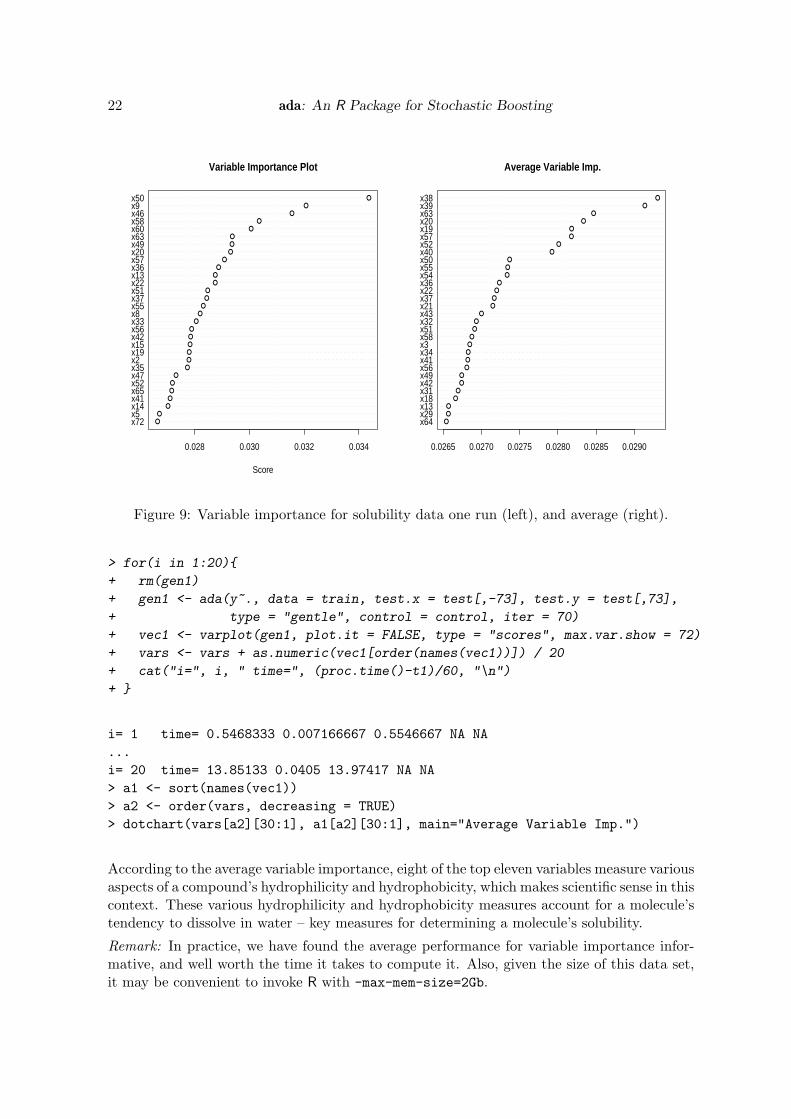
In order to enhance our understanding regarding the relationship between descriptors and theresponse, the varplot function was employed. It can be seen from Figure 9 that variable 5is the most important one.

> varplot(gen1)

The features are quite noisy and the variables are correlated, which makes variable importancedifficult to ascertain from this one run. Next we provide a small run to obtain the averagevariable importance over 20 iterations.

> vars <- rep(0,72)

> t1 <- proc.time()


x72x5x14x41x65x52x47x35x2x19x15x42x56x33x8x55x37x51x22x13x36x57x20x49x63x60x58x46x9x50

●

●

●

●

●

●

●

●

●

●

●

●

●

●

●

●

●

●

●

●

●

●

●

●

●

●

●

●

●

●

0.028 0.030 0.032 0.034

Variable Importance Plot

Score

x64x29x13x18x31x42x49x56x41x34x3x58x51x32x43x21x37x22x36x54x55x50x40x52x57x19x20x63x39x38

●

●

●

●

●

●

●

●

●

●

●

●

●

●

●

●

●

●

●

●

●

●

●

●

●

●

●

●

●

●

0.0265 0.0270 0.0275 0.0280 0.0285 0.0290

Average Variable Imp.

Figure 9: Variable importance for solubility data one run (left), and average (right).

> for(i in 1:20){

+ rm(gen1)

+ gen1 <- ada(y~., data = train, test.x = test[,-73], test.y = test[,73],

+ type = "gentle", control = control, iter = 70)

+ vec1 <- varplot(gen1, plot.it = FALSE, type = "scores", max.var.show = 72)

+ vars <- vars + as.numeric(vec1[order(names(vec1))]) / 20

+ cat("i=", i, " time=", (proc.time()-t1)/60, "\n")

+ }

i= 1 time= 0.5468333 0.007166667 0.5546667 NA NA...i= 20 time= 13.85133 0.0405 13.97417 NA NA> a1 <- sort(names(vec1))> a2 <- order(vars, decreasing = TRUE)> dotchart(vars[a2][30:1], a1[a2][30:1], main="Average Variable Imp.")

According to the average variable importance, eight of the top eleven variables measure variousaspects of a compound’s hydrophilicity and hydrophobicity, which makes scientific sense in thiscontext. These various hydrophilicity and hydrophobicity measures account for a molecule’stendency to dissolve in water – key measures for determining a molecule’s solubility.

Remark: In practice, we have found the average performance for variable importance infor-mative, and well worth the time it takes to compute it. Also, given the size of this data set,it may be convenient to invoke R with -max-mem-size=2Gb.


5.3. Stochastic boosting in a multi-class context

Currently, several boosting algorithms can not directly handle a K-class response. Thistopic constitutes an active area of research. However, several methods have been proposedin the literature to address this issue. One popular strategy is the one-versus-all tech-nique, where each individual class (typically coded as 1), is modeled against all the remain-ing classes (each coded as zero), and K different ensembles are constructed. The valuesFk(x) =

∑Mm=1 αmfm(x), k = 1, ...,K returned by each ensemble are compared and the value

corresponding to the maximum Fk is given as the class label (Friedman et al. 2000).

To illustrate the use of ada for multi-class data sets, a ten dimensional feature vector (X1, . . . , X10)was simulated from a standard normal distribution. The response variables is constructed as:

Y =

1 :

∑pr=1 X2

r ≤ χ210(.33)

2 : χ210(.33) <

∑pr=1 X2

r ≤ χ210(.66)

3 :∑p

r=1 X2r > χ2

10(.66)

This produces a three class analog to the example given above. For this example, a trainingand a testing data set which comprised of 200 and 1000 observations, respectively, weregenerated.

> n <- 1200

> p <- 10

> K <- 3

> set.seed(100)

> x <- matrix(rnorm(n * p), ncol = p)


> indtest <- setdiff(1:n, indtrain)

> val <- qchisq(c(.33, .66), 10)

> su <- apply(x^2, 1, sum)

> Iy <- cbind(as.numeric(su <= val[1]), as.numeric( val[1] < su & su <= val[2]),

+ as.numeric(su > val[2]))

> y <- apply(Iy, 1, which.max)

> test <- data.frame(y = y[indtest], x[indtest,])

A 250-iteration stochastic version of Discrete AdaBoost ensemble was constructed using de-fault trees as the base learner. The implementation of the one-versus-all strategy is givennext:

> Fs <- list()

> for(i in 1:K)

+ Fs[[i]] <- ada(y~., data = data.frame(y = Iy[indtrain, i], x[indtrain,]),

+ iter = 250,test.x = test, test.y = Iy[indtest, i])$model$F[[2]]

The in class test error rate and total test error rate will be obtained below using the sapply andtable commands in R. For more information on these commands refer to (Becker, Chambers,and Wilks 1988).

> wmx <- function(i)which.max(c(Fs[[1]][i],Fs[[2]][i],Fs[[3]][i]))

> preds <- sapply(1:1000,wmx)


> tab <- table(y[indtest],preds)

> for(i in 1:K){

+ cat("In class error rate for class ", i, ": ",

+ round(1 - tab[i,i] / sum(tab[i,]), 3), "\n")

+ }

In class error rate for class 1 : 0.281In class error rate for class 2 : 0.644In class error rate for class 3 : 0.324

> 1 - sum(diag(tab)) / length(indtest)

[1] 0.416

Notice that although the test error rate appears high, it is still substantially lower thanrandom guessing (0.66). Also the in class error rate for class two seems to be rather high.

In order to assess the magnitude of the error rate, a random forest classifier (Breiman 2001)was considered. The choice of a random forest as an ensemble method is due to its abilityto handle multi-class problems and its overall competitive performance. The following codeusing the R package randomForest constructs such an ensemble for the data at hand (Liawand Wiener 2002).

> library("randomForest")

> train <- data.frame(y=as.factor(y[indtrain]), x[indtrain,])

> set.seed(100)

> grf <- randomForest(y~., train)

> tab3 <- table(y[indtest], predict(grf, test))

> for(i in 1:K){

+ cat("In class error rate for class ", i,": ",

+ round(1 - tab3[i,i] / sum(tab[i,]), 3), "\n")

+ }

In class error rate for class 1 : 0.272In class error rate for class 2 : 0.623In class error rate for class 3 : 0.352

> 1 - sum(diag(tab3)) / length(indtest)

[1] 0.415

It can be seen that the overall test error rate (0.415) is about the same as that producedby Discrete AdaBoost, which strongly indicates that the combination of the ada and theone-versus-all strategy can easily handle multi-class classification problems.


6. Summary and concluding remarks

In this paper, the R package ada that implements several boosting algorithms is described. Itskey features are its functional modularity, the adjustment of class priors for tree classifiers,as well as the incorporation of several useful in practice plots, such as the pairs and theimportance of variables plot.

Overall, boosting has had a significant impact both in theoretical and applied research onclassification problems, as can be seen by the size of the existing literature on the topic.However, the choice of base classifiers plays a crucial role in the performance of the ensemble.Typically for 4 or 8-split trees, after a large number of iterations the training error rate isdriven to zero, while the test error decreases up to a certain level and then oscillates aroundthis level. In that respect, the performance seen in our first data example is somewhatatypical, where the training error rate has not reached zero even after 400 iterations. This ismost likely due to the use of stumps as a base classifier.

Acknowledgements

The authors would like to thank the Editor Jan de Leeuw, an Associate Editor and twoanonymous referees for useful comments and suggestions. The work of George Michailidiswas supported in part by NIH grant P41 RR18627-01 and by NSF grant DMS 0204247.

References

Becker R, Chambers J, Wilks A (1988). The New S Language: A Programming Environmentfor Data Analysis and Graphics. Wadsworth and Brooks/Cole Advanced Books & Software,Monterey, CA. ISBN 0-534-09192-X.

Boonyanunta N, Zeephongsekul P (2003). “Improving the Predictive Power of AdaBoost: ACase Study in Classifying Borrowers.” In “Proceedings of the 16th International Conferenceon Developments in Applied Artificial Intelligence,” pp. 674–685. Springer Verlag Inc. ISBN3-540-40455-4.

Breiman L (1996). “Bagging Predictors.” Machine Learning, 24(2), 123–140.doi:10.1023/A:1018054314350.

Breiman L (2001). “Random Forests.” Machine Learning, 45(1), 5–32.doi:10.1023/A:1010933404324.

Breiman L, Friedman J, Olshen R, Stone C (1984). Classification and Regression Trees.Chapman & Hall, New York.

Cohen J (1960). “A Coefficient of Agreement for Nominal Data.” Education and PsychologicalMeasurement, 20, 37–46.

Dettling M (2004). “BagBoosting for Tumor Classification with Gene Expression Data.”Bioinformatics, 20(18), 3583–3593. doi:10.1093/bioinformatics/bth447.

http://dx.doi.org/10.1023/A:1018054314350

http://dx.doi.org/10.1023/A:1010933404324

http://dx.doi.org/10.1093/bioinformatics/bth447


Freund Y, Schapire R (1996). “Experiments with a New Boosting Algorithm.” In “Interna-tional Conference on Machine Learning,” pp. 148–156.

Freund Y, Schapire R (1997). “A Decision-Theoretic Generalization of On-Line Learningand an Application to Boosting.” Journal Computer and System Sciences, 55(1), 119–139.doi:10.1006/jcss.1997.1504.

Friedman J (2001). “Greedy Function Approximation: A Gradient Boosting Machine.” TheAnnals of Statistics, 29(5), 1189–1232.

Friedman J (2002). “Stochastic Gradient Boosting.” Computational Statistics & Data Anal-ysis, 38(4), 367–378. doi:10.1016/S0167-9473(01)00065-2.

Friedman J, Hastie T, Tibshirani R (2000). “Additive Logistic Regression: A Statistical Viewof Boosting.” The Annals of Statistics, 28(2), 337–407.

Hastie T, Tibshirani R, Friedman J (2001). The Elements of Statistical Learning. SpringerVerlag. ISBN 0-387-95284-5.

Hothorn T, Buhlmann P (2006a). “Model-based Boosting in High Dimensions.” Bioinformat-ics. doi:10.1093/bioinformatics/btl462. Forthcoming.

Hothorn T, Buhlmann P (2006b). mboost: Model-based Boosting. R package version 0.4-13.

Huang K, Murphy R (2004). “Boosting Accuracy of Automated Classification of Flu-orescence Microscope Images for Location Proteomics.” BMC Bioinformatics, 5, 78.doi:10.1186/1471-2105-5-78.

Kawakita M, Minami M, Eguchi S, Lennert-Cody C (2005). “An Introduction to the Predic-tive Technique AdaBoost with a Comparison to Generalized Additive Models.” FisheriesResearch, 76(6), 323–343.

Lemmens A, Croux C (2005). “Bagging and Boosting Classification Trees to Predict Churn.”Journal of Marketing Research, 43(2), 276–268.

Liaw A, Wiener M (2002). “Classification and Regression by randomForest.” R News, 2(3),18–22. URL http://CRAN.R-project.org/doc/Rnews/.

R Development Core Team (2006). R: A Language and Environment for Statistical Computing.R Foundation for Statistical Computing, Vienna, Austria. ISBN 3-900051-07-0, URL http://www.R-project.org/.

Ridgeway G (2006). gbm: Generalized Boosted Regression Models. R package version 1.5-7,URL http://www.i-pensieri.com/gregr/gbm.shtml.

Rosset S, Zhu J, Hastie T (2004). “Boosting as a Regularized Path to a Maximum MarginClassifier.” Journal of Machine Learning Research, 5, 941–973.

Schapire R (1990). “The Strength of Weak Learnability.” Machine Learning, 5(2), 197–227.doi:10.1023/A:1022648800760.

http://dx.doi.org/10.1006/jcss.1997.1504

http://dx.doi.org/10.1016/S0167-9473(01)00065-2

http://dx.doi.org/10.1093/bioinformatics/btl462

http://dx.doi.org/10.1186/1471-2105-5-78

http://CRAN.R-project.org/doc/Rnews/

http://www.R-project.org/

http://www.R-project.org/

http://www.i-pensieri.com/gregr/gbm.shtml

http://dx.doi.org/10.1023/A:1022648800760


Segal M (2004). “Machine Learning Benchmarks and Random Forest Regression.” Technicalreport, Center for Bioinformatics & Molecular Biostatistics, University of California, SanFrancisco, CA. URL http://repositories.cdlib.org/cbmb/bench_rf_regn/.

Sugata S, Abe Y (2001). “Computer Simulation of Hydrodynamic Models forChemical/Pharmaco-Kinetics.” Journal of Chemical Software, 7(2).

Therneau T, Atkinson B (2005). rpart: Recursive Partitioning Software. R pack-age version 3.1-32, URL http://mayoresearch.mayo.edu/mayo/research/biostat/splusfunctions.cfm.

Ulintz P, Zhu J, Qin Z, Andrews P (2006). “Improved Classification of Mass Spectrome-try Database Search Results Using Newer Machine Learning Approaches.” Molecular andCellular Proteomics, 5(3), 497–509.

Valiant L (1984). “A Theory of The Learnable.” In “Proceedings of the 16th Annual ACMSymposium on Theory of Computing,” pp. 436–445. ACM Press, New York, NY. ISBN0-89791-133-4. doi:10.1145/800057.808710.

Affiliation:

Mark CulpDepartment of StatisticsUniversity of Michigan436 West Hall, 550 East UniversityAnn Arbor, MI 48109, United States of AmericaE-mail: [email protected]: http://www.stat.lsa.umich.edu/~culpm/

Kjell JohnsonE-mail: [email protected]

George MichailidisE-mail: [email protected]: http://www.stat.lsa.umich.edu/~gmichail/

Journal of Statistical Software http://www.jstatsoft.org/published by the American Statistical Association http://www.amstat.org/

Volume 17, Issue 2 Submitted: 2005-07-13October 2006 Accepted: 2006-09-26

http://repositories.cdlib.org/cbmb/bench_rf_regn/

http://mayoresearch.mayo.edu/mayo/research/biostat/splusfunctions.cfm

http://mayoresearch.mayo.edu/mayo/research/biostat/splusfunctions.cfm

http://dx.doi.org/10.1145/800057.808710

mailto:[email protected]

http://www.stat.lsa.umich.edu/~culpm/



http://www.stat.lsa.umich.edu/~gmichail/

http://www.jstatsoft.org/

http://www.amstat.org/

ada: an r package for stochastic boosting · the underlying engine is the rpart ... an r package...

Documents