adam f. wallace ([email protected]) & kendra j. lynn ( kjlynn
TRANSCRIPT
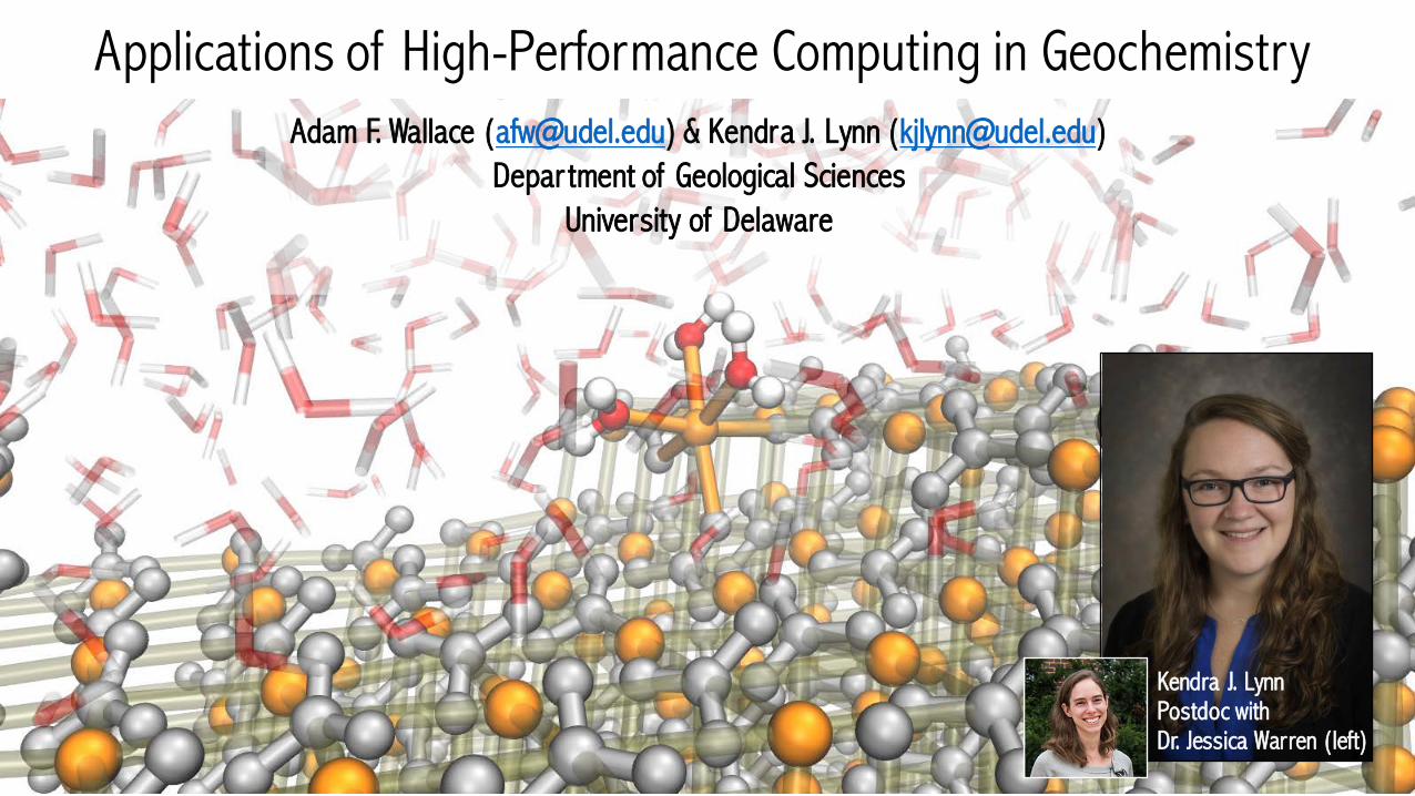
Adam F. Wallace ([email protected]) & Kendra J. Lynn ([email protected])Depar tment of Geological Sciences
University of Delaware
Applications of High-Performance Computing in Geochemistry
Kendra J. LynnPostdoc with Dr. Jessica Warren (left)

LabMembersandAffiliates
AdamWallace
Yifei MaPh.D.student
JuneHazewskiM.S.student
ChunleiWangPh.D.student(Sturchio Lab)
BriannaMcEvoyM.S.2017

Geochemistsareinterestedinprocessesthatoccuroverawidevarietyoftimeandlengthscales
AtomicScale MineralSurfaces GrainBoundaryProcesses
WholeRockRegional
Global
2.5 x 2.5 µm

QC(ab initio/DFT)
ReactiveMD(i.e.ReaxFF)
MD
CoarseGrained
Continuum
Distance
Time
ion-ionion-water
gas-water
ion-hydrolysis/polymerizationIonsorption/desorptionDiffusioninsolution
nucleation/growthrecrystallizationmineral-waterequilibria
pore-scalewholemineral/rockregionalscale
Modelingiscriticalbecausemanylocationsandconditionsofinterestarephysicallyinaccessibleinthefieldandinthelab
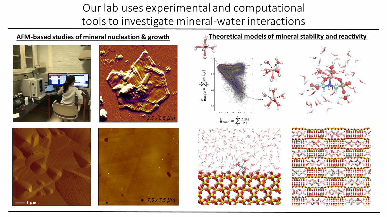
Ourlabusesexperimentalandcomputationaltoolstoinvestigatemineral-waterinteractions
AFM-basedstudiesofmineralnucleation&growth
7.5 x 7.5 µm
2.5 x 2.5 µm
Σ3 i
cos θr ir
iξ a
ngle
=
Σ3
i
ri rir0
2ξbond =
Theoreticalmodelsofmineralstabilityandreactivity

• DensityFunctionalTheory(DFT),abinitiomethods
• BasedonapproximatesolutionstoSchrodinger’s equation:
• Physicsmodeledwith“high”accuracy.
• Requiresalotofcomputerpower.
• 10-20ps trajectoriestypical
Overviewofatomisticsimulationmethods
HΨ =EΨ
ElectronicStructureMethods
• BasedonNewton’sequationsofmotion.
• Physicsmodeledwithwithlessprecision.
• Requiresalotofcomputerpowerbutlessthanelectronicstructuremethods.
• 10-100nstrajectoriestypical
ClassicalMolecularDynamics
F=ma

Reactionsofgeochemicalinterestareoftentooslowtobeobservedwithdirectsimulationmethods
• Earth’scrustisprimarilycomposedofsilicateminerals
• Atsurfaceconditionsmostsilicatesdissolvevery
slowly(10-6 to10-14 mol /m2 sec).
• Evenat200°Cquartzdissolvesat~10-6 mol /m2 secin
saltwatersolutions.
Dove and Nix (2002) GCA, 61:3329-3340.
Thisisequivalenttothereleaseof~10-4 moleculesof
H4SiO4° per100nm2 ofsurfacepermicrosecond.

Specializedmethodsareneededtoovercometimescalelimitationsandenhancesampling
• MinimaHopping(LJ38)• ReplicaExchangeMolecularDynamics(CaCO3.nH2Oclusters)
Globalenergyminimizationstrategies
• UseoftheColvars LibraryinLAMMPS• UmbrellaSampling(waterexchangeonCa2+)• Metadynamics (Si-Obondhydrolysis)
Explorationoffreeenergylandscapeswithbiaseddynamics
• Directmethods• ReactiveFlux• ForwardFluxSampling
Calculationofreactionrates(waterexchangereactions)
• 2PT(substitutionofCO2 forH2Oinsepiolite)AbsoluteFreeEnergymethods

GlobalEnergy
MinimizationStrategies

MinimaHopping (Goedecker (2004) J. Chem. Phys., 120:9911)
• Hoppingisperformedbyactivation-relaxationsteps.
• Duringanactivationstep,amoleculardynamicstrajectoryisinitiatedwithagivenkineticenergy(Ekin)andfolloweduntilthepotentialenergydecreases.
• Duringarelaxationstepthesystemenergyisminimized tothenearestlocalminimum.
• Themovetothenewminimumisacceptediftheenergydifferencebetweenthenewandoldminimaislessthanaparameter(Ediff)thatisdynamicallyadjustedsothat~50%ofthemovesareaccepted.
• IfthesystemreturnstoaminimumithasalreadyvisitedEkin isincreased.
PotentialEne
rgy
ReactionProgress
FailedescapeEkin increases
SuccessfulescapeEkin decreases

MinimaHopping (Goedecker (2004) J. Chem. Phys., 120:9911)
• ActivationstepsareperformedwithLAMMPS• RelaxationstepsareperformedwithLAMMPSorGULP.• Apythonscriptcontrolsthesetupandexecutionof
LAMMPS/GULP.
ImplementationDetails
Energy
MinimaVisited

Exchangebetweenreplicasoccurssubjecttoaconditionalprobabilityrule.
ParallelTempering/ReplicaExchangeMolecularDynamics

Potential Energy Landscape
ReplicaExchangeSamplingCircumventsHighEnergyBarriers

Potential Energy Landscape
ReplicaExchangeSamplingCanLocateGlobalMinima

EnhancedsamplingofhydratedCaCO3 clusterswithReplicaExchangeMolecularDynamics().Wallace et al. (2013) Science, 341:885-889

ExplorationofFreeEnergy
LandscapeswithBiasedDynamics

UseoftheColvars LibraryinLAMMPS
• TheColvars libraryisincludedinLAMMPSdistributionsasanoptionalpackage.
• Thelibraryenablesanumberofbiasedsamplingmethods,including:umbrellasampling,metadynamicsandadaptivebiasforce.
• Thelibraryisinvokedasa“fix”intheLAMMPSinputscript.

AnatomyofasimpleCOLVARSinputfile
Blockthatdefinesthecollectivevariabletoapplythebiasto.Inthiscasethedistancebetweentwogroupscontaining1atomeach.
Outputandrestartfrequency.
Thisblockappliesaharmonicrestrainingpotentialtomaintainthevalueofthecollectivevariable“DIST”centeredaround3.1.Theenergyunitsarethoseusedbylammps.InthiscasetheforceconstantisineV.

SampleCOLVARSOutput
Instantaneousvalueof“DIST”MDStep

Obtainingthefreeenergybarrier(UmbrellaSampling)
Definereactionprogresscoordinate(oftenmetal-oxygendistanceforwaterexchangereactions)
1 2 Applyabiasalongthereactioncoordinate
3 Obtainbiasedprobabilitydistributions
4 Convertprobabilities tofreeenergiesforeachwindowandsubtractthebiaspotential.
5 Combine freeenergysegments

UsingWHAMutilitytoProcessCOLVARSOutput
WeuseautilitymaintainedbyAlanGrossfield atU.RochestertoprocessumbrellasamplingoutputfromCOLVARS.
http://membrane.urmc.rochester.edu/content/wham
Theutilitytakesafile”metadata”asinputthatspecifiesthelocationsoftheCOLVARSoutputforallthesamplingwindows,andwritesanoutputfile”freefile”thatcontainsthefreeenergywithrespecttothebiasescoordinate.

UsingWHAMutilitytoProcessCOLVARSOutput
PathtoCOLVARSoutputfileswindowcenter
Restraintforce
constant(kcal/mol)
Samplemetadatafile
RunningWHAM

Van Speybroeck et al. (2014) Chem. Soc. Rev., 43:7326-7357.
Metadynamics Basics
Themetadynamics methodacceleratestheexplorationofenergylandscapesbytheslowbuildupofahistorydependentbias.
Thebiasencouragesthesimulationtoexplorenewstatesandultimatelygrowstoformthenegativeimageoftheenergylandscape.

min(Si-OW)
max(Si-O
br)
Metadynamics SimulationofSi-OBondHydrolysis

SampleLAMMPSandCOLVARSinputfilesfor2DMetadynamics
LAMMPSInput COLVARSInput
LAMMPSgroupswrittentofiletobereadbyCOLVARS
Filetoreadgroupdefinitions from
Definitionofcollectivevariable“one”astheminimumSi-OW distance.
Definitionofcollectivevariable“two”asthemaximumSi-Obr distance.ThisusesacustomfunctionthatdependsontheLeptonlibrary.
Settingsthatcontroltheaccumulationofthemetadynamicsbiasfunction.

Calculation
WaterExchangeRates

!I# H%O '] + H%O∗+,- [I# H%O '/0 H%O∗]+ H%O
Richens (2005) Chem. Rev., 105(6):1961-2002.
𝜏234 =1𝑘38

CorrelationofWaterExchangeRates&BulkReactivityTrends
Casey (2017) Adv. Inorg. Chem., 69:91-115.
Comp.by:
DElaya
raja
Stage:Proof
ChapterNo.:27
Title
Name:ADIO
CH
Date:12/1/17
Tim
e:15:36:32
PageNumber:5
Fig. 2f0010 Dissolution rates at pH 2 of simple oxide (A) and orthosilicate (B and C) minerals containing divalent metals. The abscissa is the rate ofexchange of water from the corresponding metal ion (e.g., Mg2+(aq)), and the ordinate is the dissolution rate of the mineral (e.g., Mg2SiO4,forsterite) normalized to area. The oxide minerals have the rocksalt structure. The orthosilicate minerals (5) have the stoichiometry:M2SiO4(s) and isolated SiO4
4! tetrahedra. The end-member compositions of orthosilicates are shown in red squares in (B), whereas themixed-metal compositions are shown as blue dots. For the mixed-metal compositions, dissolution rates are plotted against the weightedsum of the logarithm of rates of water exchange for the component ions. Note that the dissolution rates for mixed-metal compositions (bluedots in (B)) fall intermediate between the end-member compositions. The rates of ligand exchange of the aquated ions ( ) and the dissolutionrates of the orthosilicate minerals ( ) at pH 2 are plotted as a function of the number of d electrons in (C), illustrating the role of ligand-fieldstabilization in the rates. Panels (B) and (C) are adapted from Ref. Casey, W.H.; Swaddle, T.W. Reviews of Geophysics 2003, 41 (2), 4/1–4/20.
To protect the rights of the author(s) and publisher we inform
you that this PDF is an uncorrected proof for internal business use only
by the author(s), editor(s), reviewer(s), Elsevier and typesetter SPi. It is not allow
ed to publish this proof online or in print. This proofcopy is the copyright property of the publisher and is confidential until form
al publication.
These proofs may contain colour figures. Those figures m
ay print black and white in the final printed book if a colour print product
has not been planned. The colour figures will appear in colour in all electronic versions of this book.
(OxidesandOrthosilicates)

Dove and Nix (2002) GCA, 61:3329-3340.
(SiO2)3338 P .M. Dove and C.J. Nix
(a)
o
= ©
_= @
~3 o ©
©
(b)
0
O
©
@
o
-6.0
-6.5
-7.0
-7.5
-8.0 0.00
[] water, electrolytes not present • 0.01 molal M e C 1 2 ~ 2 © 0.05 molal MeC12 o
q
2+
[]
Si 4+ 200oC i I r I i I I I r i i [ i ~ i i i i r
2.00 4.00 6.00 8.00 10.00 log kex of aqueous ions (s -1)
-6.0
-6.5
-7.0
-7.5
-8.0 0.00
[] water, electrolytes not present
[] []
200°C i K i I i i I I i i i I i i i I i r i
2.00 4.00 6.00 8.00 10.00
log kex of aqueous ions (s -1)
Fig. 5. Dissolution rate of quartz at 200°C vs. log rate of solvent exchange, kox, for the predominant cation at the silica-solution interface. Slowest rates are measured in salt-free solutions where only low concentrations H4SiO4, is present. Rates increase with the introduction of IIA cations in a predictable trend that is linearly related to their kex value. (a) A comparison of rates measured in 0.01 and 0.05 molal solutions shows that the slopes of these linear relationships increase with the total MeClz concentration. Trends have r 2 of 0.996 and 0.983, respectively. (b) Quartz dissolution rates in solutions containing one of six different monovalent and divalent cations having comparable ionic strengths of 0.15 show an empirical correlation given by Eqn. 10.
studies of amorphous and crystalline silica polymorphs which suggests that these relative rates hold over the temperature range of 20-200°C. In the broader perspective of Earth envi- ronments, any of these IA or IIA cations have a greater rate enhancing effect than organic compounds. For example, Ben- nett et al. (1988) and Bennett (1991) showed that organic acids, citrate, and oxalate, enhanced quartz dissolution rates by
a factor of two compared to pure water. In contrast, solutions containing potassium or barium ion can enhance rates as much as forty times at 200°C.
5.1. Relationship to Previous Studies The relationship between quartz dissolution rate and the
kex of solute ions shown in Fig. 5a,b is consistent with previ-
CorrelationofWaterExchangeRates&BulkReactivityTrends

Pokrovsky and Schott (2002) Environ. Sci. Technol., 36:426-432.
(Carbonates)CorrelationofWaterExchangeRates&BulkReactivityTrends

5
7
6
1
3
4
2
DirectRateMethodsforLigandSubstitution
𝜏234 =1𝑘38
= 9 𝑅(𝑡) 𝑑𝑡?
@
(Impey’s Method)
1
2
3
45
67 𝑅(𝑡) =
1𝑛(0)
C𝜃E(0)𝜃E(𝑡)'(F)
EG0
Ca2+
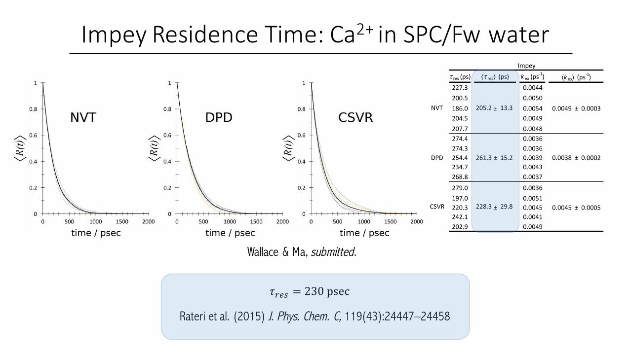
Impey ResidenceTime:Ca2+inSPC/Fw waterτ res(ps) k ex(ps
-1)227.3 0.0044200.5 0.0050186.0 ± 0.0054 0.0049 ± 0.0003204.5 0.0049207.7 0.0048274.4 0.0036274.3 0.0036254.4 ± 0.0039 0.0038 ± 0.0002234.7 0.0043268.8 0.0037279.0 0.0036197.0 0.0051220.3 ± 0.0045 0.0045 ± 0.0005242.1 0.0041202.9 0.0049
Impey
⟨k ex⟩(ps-1)⟨τ res⟩(ps)
NVT 205.2 13.3
DPD 15.2
CSVR 228.3 29.8
261.3
Wallace & Ma, submitted.
Rateri et al. (2015) J. Phys. Chem. C, 119(43):24447–24458
𝜏234 = 230psec

DirectRateMethodsforLigandSubstitution(Hofer’s “Direct” Method)
RESERVOIR𝑟E' 𝑟PQF
𝑟E' = 𝑟PQF = massexchangerate
𝜏234 =ReservoirMass
MassExchangeRate

DirectRateMethodsforLigandSubstitution(Hofer’s “Direct” Method)
𝜏234 =ReservoirMass
MassExchangeRate
ReservoirMass = 𝑛(ioncoordinationnumber)
MassExchangeRate = 𝑟38 =numberofexchangesperion
lengthofsimulation
𝜏234 =1𝑘38
=𝑛
𝑟38 Ca%f⁄

Indirectratemethods(ReactiveFlux)
𝑘hi = 𝜅𝑘klk
FreeEne
rgy
ReactionProgress
ΔG*Transitionstatetheoryrateconstant(determinedbytheheightoftheenergybarrier)
Transmissioncoefficient(dynamicalcorrectionto𝑘klk)
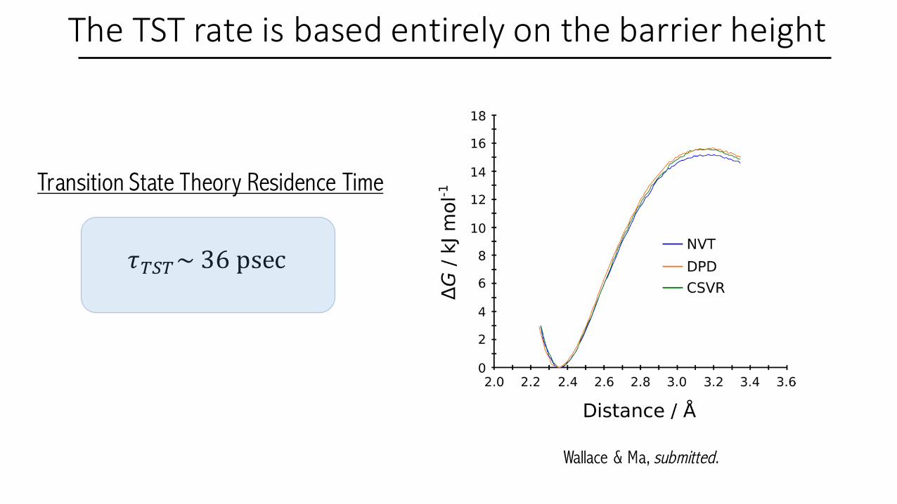
TheTSTrateisbasedentirelyonthebarrierheight
Wallace & Ma, submitted.
Transition State Theory Residence Time
𝜏klk~36psec

TSTassumeseveryvisittothetransitionstateissuccessful(thisisn’tture)
𝜅 𝑡 =�̇� 0 𝜃[𝑟 𝑡 − 𝑟‡r s�̇� 0 𝜃[�̇�(0)] s
TocorrecttheTSTratewecalculatethetransmissioncoefficient:
NumberofsuccessfultrajectoriesTotalnumberofattempts 0
0.2
0.4
0.6
0.8
1
0 0.5 1 1.5 2
k(t)
Time(psec)

k TST(ps-1)
NVT 0.0322 0.1748 ± 0.0062 0.0056 ± 0.0002 178.1 ± 7.0DPD 0.0273 0.1678 ± 0.0211 0.0046 ± 0.0006 221.4 ± 31.2CSVR 0.0257 0.1707 ± 0.0213 0.0044 ± 0.0005 231.4 ± 34.3
ReactiveFlux
k k RF(ps-1) t RF(ps)
ApplyingthedynamicalcorrectionyieldsτRF≈ τres
Wallace & Ma, submitted.
0
0.2
0.4
0.6
0.8
1
0 0.5 1 1.5 20
0.2
0.4
0.6
0.8
1
0 0.5 1 1.5 20
0.2
0.4
0.6
0.8
1
0 0.5 1 1.5 2
K(t)
Time(psec) Time(psec) Time(psec)
CSVRDPDNVT
𝑘hi =1𝜏hi
= 𝜅𝑘klk

Indirectratemethods(ForwardFluxSampling)AttemptRateCalculation DeterminationofInterfaceFluxes
𝑃 𝜆w 𝜆@) =x𝑃 𝜆Ef0 𝜆E)'/0
EG@𝑘iil =
1𝜏iil
= Φz{,w = Φz{,}~𝑃 𝜆w 𝜆@)

Elapsedtimeisusedintheplaceofatraditionalorderparameter
𝑛 = CC𝑠E� 𝑟�E
• Variablepathlength• Influenceoforderparameterminimized• Definingproduct stateisnotnecessary
(enablesunguided searchesformetastablestates)
Thetransitioninterfacesaredefinedwithrespecttotheamountoftimeelapsedoutsidethereactantbasin.
PotentialAdvantages:
Reactant/Productbasinsaredefinedbythresholdvaluesofn:

TypicalConvergenceBehavioroftheInterfaceCrossingProbabilities
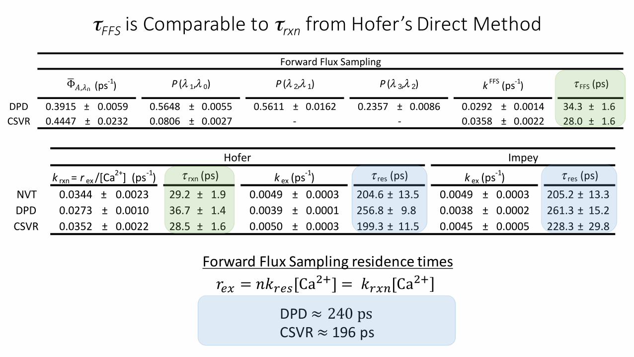
τFFS isComparabletoτrxn fromHofer’sDirectMethod
DPD 0.3915 ± 0.0059 0.5648 ± 0.0055 0.5611 ± 0.0162 0.2357 ± 0.0086 0.0292 ± 0.0014 34.3 ± 1.6CSVR 0.4447 ± 0.0232 0.0806 ± 0.0027 - - 0.0358 ± 0.0022 28.0 ± 1.6
τ FFS(ps)
ForwardFluxSampling
(ps-1) P (λ 1,λ 0) P (λ 2,λ 1) P (λ 3,λ 2) k FFS(ps-1)Φ"#,%0
NVT 0.0344 ± 0.0023 29.2 ± 1.9 0.0049 ± 0.0003 204.6 ± 13.5 0.0049 ± 0.0003 205.2 ± 13.3DPD 0.0273 ± 0.0010 36.7 ± 1.4 0.0039 ± 0.0001 256.8 ± 9.8 0.0038 ± 0.0002 261.3 ± 15.2CSVR 0.0352 ± 0.0022 28.5 ± 1.6 0.0050 ± 0.0003 199.3 ± 11.5 0.0045 ± 0.0005 228.3 ± 29.8
τ res(ps)Impey
k rxn=r ex/[Ca2+](ps-1) τ rxn(ps) k ex(ps
-1) τ res(ps)Hofer
k ex(ps-1)
𝑟38 = 𝑛𝑘234[Ca%f] = 𝑘28'[Ca%f]ForwardFluxSamplingresidencetimes
DPD≈ 240psCSVR≈ 196ps

LookingTowardstheFuture
Student/Postdoc OpportunitiesContact: [email protected]
ξbond dominated
ξbond andξangle

MODELING THE COMPOSITIONAL ZONING OF MINERALS
A GEOCHEMICAL TOOL FOR INVESTIGATING THE
TIMESCALES OF EARTH PROCESSES
Kendra J. Lynn

DIFFUSION CHRONOMETRY
• Minerals in rocks can be used to calculate the timescales of Earth processes
Rosen (2016)

CHEMICAL ZONING: OLIVINE
Rosen (2016)
a) Initially homogeneous core of composition X
b) Secondary growth of a crystal rim with composition Y
c) Chemical diffusion between core and rim -
d) System attempts to reach equilibrium between compositions X and Y

MODELING CHEMICAL ZONING
• Goal: Model diffusive re-equilibration in 3D

MODELING CHEMICAL ZONING
• Goal: Model diffusive re-equilibration in 3D
Zoning patterns are directly related to
storage time.
!"!# =
!!% & !"!%
Crank (1975)
• Finite difference, forward time, centered space discretization
• Fick’s second Law: Continuity equation

DIFFUSION ANISOTROPY
• Diffusion is anisotropic
• Da=Db=1/6Dc
Shea et al. 2015

DIFFUSION ANISOTROPY
• Diffusion is anisotropic
• Da=Db=1/6Dc
Dtrav = Da(cosα)2 + Db(cosβ)2 + Dc(cosγ)2
Shea et al. 2015

MODELING MULTIPLE ELEMENTS
best-fit
Modeling multiple elements in parallel is computationally expensive

ZONING IN THREE DIMENSIONS

ZONING IN THREE DIMENSIONS
Stability Criterion – where R < 0.166
• To maintain a high spatial resolution (small ∆x), each timestep iteration (∆t) must also be small
• High resolution diffusion models are time intensive, requiring high performance computing

SUMMARY
• Current 3D models require 1 month to simulate 3 elements on desktop computer with 32 GB RAM
• The same models are run in < 8 hours on Farber
• Future plans to model 3 different minerals with many elements each at the same time
PleasecontactKendraJ.Lynn([email protected])