adaptive beamforming for next generation cellular...
TRANSCRIPT
DEPARTMENT OF ELECTRICAL AND INFORMATION TECHNOLOGY
FACULTY OF ENGINEERING | LTH | LUND UNIVERSITY
SE-221 00 LUND, SWEDEN
Adaptive Beamforming for NextGeneration Cellular System
Sebastian Andersson [email protected] Tidelund [email protected]
September 16, 2016
SupervisorsFredrik Tufvesson [email protected] Venkatraman Bhat [email protected]
EricssonMobilvägen 1, 224 71 Lund

ABSTRACT
In this work a Matlab model of a simplified LTE system has been implemented. ThePUSCH and PDSCH signal chains has been used for reception and transmission ofdata and DM-RS symbols are used as pilots. Moreover, the model supports com-munication and interference between multiple users and base station antennas.The wireless channels are modeled as multi-path Rayleigh fading and are continu-ous in time such that multiple frames can be transmitted on a correlated channel.Three standardized multi-path delay profiles have been used for modeling users inpedestrian, vehicular and urban environments. Three beamforming algorithms havebeen implemented, maximum ratio transmission, zero-forcing and regularized zero-forcing. This model is an extension to the current standard of LTE in the sense that theparameters of the model are scalable beyond what is currently in the standard. Thedifferent algorithms are compared in many different scenarios, including differentmodulation levels, delay profiles, number of user sharing the same resources, numberof base station antennas, multi-layer transmissions and complexity. Maximum ratiotransmission is shown to be computationally less complex, while the zero-forcingalgorithms is better at removing inter-user interference, especially as the numberof users sharing the same resources grows for a constant number of base stationantennas. Regularized zero-forcing is shown to outperform the other algorithmswhen looking at the entire SNR range.
i

ACKNOWLEDGEMENTS
We would like to thank Marcus Wiedner, Harish Venkatraman Bhat, Johan Åman andChrister Östberg who gave us the opportunity to do this Master’s thesis at Ericssonand who also provided us with valuable feedback during the work. Also a big thanks toFredrik Tufvesson and his inputs to the thesis work as one of the leading researchersin this area. We are glad that we had the opportunity to do our thesis in this area eventhough our knowledge in telecommunications was limited before starting, becausewe’ve learned so much of this ever-expanding subject.
Finally a big thanks to family and friends who have supported us during the en-tire time of studies.
William Tidelund & Sebastian Andersson
ii

CONTENTS
1 Introduction 11.1 Purpose & Aims . . . . . . . . . . . . . . . . . . . . . . . . . . . . . . . . . 11.2 Methodology . . . . . . . . . . . . . . . . . . . . . . . . . . . . . . . . . . . 11.3 Limitations . . . . . . . . . . . . . . . . . . . . . . . . . . . . . . . . . . . . 21.4 Literature Study . . . . . . . . . . . . . . . . . . . . . . . . . . . . . . . . . 2
2 Background 32.1 Uplink and Downlink . . . . . . . . . . . . . . . . . . . . . . . . . . . . . . 32.2 LTE Resources . . . . . . . . . . . . . . . . . . . . . . . . . . . . . . . . . . 42.3 Transmission of User Data . . . . . . . . . . . . . . . . . . . . . . . . . . . 52.4 Reception of User Data . . . . . . . . . . . . . . . . . . . . . . . . . . . . . 82.5 Reference Signals . . . . . . . . . . . . . . . . . . . . . . . . . . . . . . . . 9
3 Wireless Channel 113.1 Channel Model . . . . . . . . . . . . . . . . . . . . . . . . . . . . . . . . . 11
3.1.1 Fading Model . . . . . . . . . . . . . . . . . . . . . . . . . . . . . . 113.1.2 Time Correlation . . . . . . . . . . . . . . . . . . . . . . . . . . . . 123.1.3 Filter Structure & Spatial Correlation . . . . . . . . . . . . . . . . 133.1.4 Large Scale Fading . . . . . . . . . . . . . . . . . . . . . . . . . . . 153.1.5 Path Loss . . . . . . . . . . . . . . . . . . . . . . . . . . . . . . . . . 15
3.2 Uplink and Downlink Reciprocity . . . . . . . . . . . . . . . . . . . . . . 153.3 Noise . . . . . . . . . . . . . . . . . . . . . . . . . . . . . . . . . . . . . . . 163.4 Coherence Time . . . . . . . . . . . . . . . . . . . . . . . . . . . . . . . . . 16
4 Downlink Beamforming 174.1 Maximum Ratio Transmission . . . . . . . . . . . . . . . . . . . . . . . . 194.2 Zero-Forcing . . . . . . . . . . . . . . . . . . . . . . . . . . . . . . . . . . . 194.3 Regularized Zero-Forcing . . . . . . . . . . . . . . . . . . . . . . . . . . . 204.4 Massive MIMO . . . . . . . . . . . . . . . . . . . . . . . . . . . . . . . . . 204.5 Power Allocation . . . . . . . . . . . . . . . . . . . . . . . . . . . . . . . . 20
5 Modeling Using LTE System Toolbox in Matlab 235.1 Interface . . . . . . . . . . . . . . . . . . . . . . . . . . . . . . . . . . . . . 23
5.1.1 Channel Setup . . . . . . . . . . . . . . . . . . . . . . . . . . . . . . 245.1.2 Link Setup and Transmission . . . . . . . . . . . . . . . . . . . . . 24
5.2 Uplink . . . . . . . . . . . . . . . . . . . . . . . . . . . . . . . . . . . . . . 255.3 Channel . . . . . . . . . . . . . . . . . . . . . . . . . . . . . . . . . . . . . 255.4 Downlink . . . . . . . . . . . . . . . . . . . . . . . . . . . . . . . . . . . . . 28
6 Results 296.1 Throughput and Validation . . . . . . . . . . . . . . . . . . . . . . . . . . 296.2 Performance in Massive MIMO . . . . . . . . . . . . . . . . . . . . . . . . 336.3 Multi-Layer Transmission . . . . . . . . . . . . . . . . . . . . . . . . . . . 346.4 Transmission of Consecutive Frames . . . . . . . . . . . . . . . . . . . . 356.5 Algorithm Complexity . . . . . . . . . . . . . . . . . . . . . . . . . . . . . 37
4
6.6 Effects of Channel Discrepancies Between Users . . . . . . . . . . . . . 376.7 Algorithm Performance and SNR . . . . . . . . . . . . . . . . . . . . . . . 396.8 Antenna Correlation . . . . . . . . . . . . . . . . . . . . . . . . . . . . . . 406.9 Mobility . . . . . . . . . . . . . . . . . . . . . . . . . . . . . . . . . . . . . 406.10 Effects of Large Scale Fading . . . . . . . . . . . . . . . . . . . . . . . . . 42
7 Discussion 437.1 Conclusion . . . . . . . . . . . . . . . . . . . . . . . . . . . . . . . . . . . . 447.2 Future work . . . . . . . . . . . . . . . . . . . . . . . . . . . . . . . . . . . 44
iii
LIST OF FIGURES
1 Illustration of a LTE radio frame and its subcomponents, [8]. . . . . . . 42 Six users in a 1.4 MHz bandwidth subframe. . . . . . . . . . . . . . . . . 53 Transmitter chain [13]. . . . . . . . . . . . . . . . . . . . . . . . . . . . . . 64 Constellation diagram QPSK. . . . . . . . . . . . . . . . . . . . . . . . . . 65 Constellation diagram 16QAM. . . . . . . . . . . . . . . . . . . . . . . . . 66 Constellation diagram 64QAM. . . . . . . . . . . . . . . . . . . . . . . . . 77 Constellation diagram 256QAM. . . . . . . . . . . . . . . . . . . . . . . . 78 Receiver chain [13]. . . . . . . . . . . . . . . . . . . . . . . . . . . . . . . . 89 User allocation for six users in a 1.4 MHz bandwidth UL subframe. . . . 1010 Signal envelope for 0.1 seconds with a maximum Doppler frequency of
70 Hz. . . . . . . . . . . . . . . . . . . . . . . . . . . . . . . . . . . . . . . . 1311 Signal envelope for 0.1 seconds with a maximum Doppler frequency of
300 Hz. . . . . . . . . . . . . . . . . . . . . . . . . . . . . . . . . . . . . . . 1312 MIMO channel between one user and base station. . . . . . . . . . . . . 1313 Time-varying FIR filter structure used for the channel. . . . . . . . . . . 1414 GUI. . . . . . . . . . . . . . . . . . . . . . . . . . . . . . . . . . . . . . . . . 2315 The program flow of the channel model, "LTEStep" in context. . . . . . 2716 Spectral efficiency as a function of UEs with QPSK and 32 ENB antennas
on an EPA channel. . . . . . . . . . . . . . . . . . . . . . . . . . . . . . . . 3017 Spectral efficiency as a function of UEs with 256QAM and 32 ENB an-
tennas on an EPA channel. . . . . . . . . . . . . . . . . . . . . . . . . . . 3018 Spectral efficiency as a function of UEs with QPSK and 32 ENB antennas
on an EVA channel. . . . . . . . . . . . . . . . . . . . . . . . . . . . . . . . 3019 Spectral efficiency as a function of UEs with 256QAM and 32 ENB an-
tennas on an EVA channel. . . . . . . . . . . . . . . . . . . . . . . . . . . 3020 Spectral efficiency as a function of UEs with QPSK and 32 ENB antennas
on an ETU channel. . . . . . . . . . . . . . . . . . . . . . . . . . . . . . . . 3121 Spectral efficiency as a function of UEs with 256QAM and 32 ENB an-
tennas on an ETU channel. . . . . . . . . . . . . . . . . . . . . . . . . . . 3122 BER as a function of UEs with QPSK and 32 ENB antennas on an EPA
channel. . . . . . . . . . . . . . . . . . . . . . . . . . . . . . . . . . . . . . 3223 BER as a function of UEs with 256QAM and 32 ENB antennas on an EPA
channel. . . . . . . . . . . . . . . . . . . . . . . . . . . . . . . . . . . . . . 3224 BER as a function of UEs with QPSK and 32 ENB antennas on an EVA
channel. . . . . . . . . . . . . . . . . . . . . . . . . . . . . . . . . . . . . . 3225 BER as a function of UEs with 256QAM and 32 ENB antennas on an EVA
channel. . . . . . . . . . . . . . . . . . . . . . . . . . . . . . . . . . . . . . 3226 BER as a function of UEs with QPSK and 32 ENB antennas on an ETU
channel. . . . . . . . . . . . . . . . . . . . . . . . . . . . . . . . . . . . . . 3327 BER as a function of UEs with 256QAM and 32 ENB antennas on an
ETU channel. . . . . . . . . . . . . . . . . . . . . . . . . . . . . . . . . . . 3328 Spectral efficiency for 4 UEs with QPSK on an EPA channel as the num-
ber of ENB antennas grows. . . . . . . . . . . . . . . . . . . . . . . . . . . 33
iv

29 Spectral efficiency for 4 UEs with QPSK on an EVA channel as the num-ber of ENB antennas grows. . . . . . . . . . . . . . . . . . . . . . . . . . . 33
30 Spectral efficiency for 4 UEs with QPSK on an ETU channel as thenumber of ENB antennas grows. . . . . . . . . . . . . . . . . . . . . . . . 34
31 Spectral efficiency for 4 UEs using QPSK and 32 antennas on an EPAchannel as the number of layers increases. . . . . . . . . . . . . . . . . . 35
32 Spectral efficiency for 4 UEs using QPSK and 32 antennas on an EVAchannel as the number of layers increases. . . . . . . . . . . . . . . . . . 35
33 Spectral efficiency for 4 UEs using QPSK and 16 antennas on an EPAchannel as the number of layers increases. . . . . . . . . . . . . . . . . . 35
34 Spectral efficiency for 4 UEs using QPSK and 16 antennas on an EVAchannel as the number of layers increases. . . . . . . . . . . . . . . . . . 35
35 The DL BER with QPSK on an EVA channel as a function of consecutiveDL frames. . . . . . . . . . . . . . . . . . . . . . . . . . . . . . . . . . . . . 36
36 The DL BER with QPSK on an ETU channel as a function of consecutiveDL frames. . . . . . . . . . . . . . . . . . . . . . . . . . . . . . . . . . . . . 36
37 The DL BER using QPSK on an EVA channel as a function of subframeswhen the weights are updated every third subframe. . . . . . . . . . . . 36
38 The DL BER using QPSK on an ETU channel as a function of subframeswhen the weights are updated every third subframe. . . . . . . . . . . . 36
39 Computation time as the number of UEs and ENB antenns grows. . . . 3740 Received constellation of user 1 in a system with two users close to the
base station. . . . . . . . . . . . . . . . . . . . . . . . . . . . . . . . . . . . 3841 Received constellation of user 2 in a system with two users close to the
base station. . . . . . . . . . . . . . . . . . . . . . . . . . . . . . . . . . . . 3842 Received constellation of user 1 in a system with one user close to the
base station and one further away. . . . . . . . . . . . . . . . . . . . . . . 3843 Received constellation of user 2 in a system with one user close to the
base station and one further away. . . . . . . . . . . . . . . . . . . . . . . 3844 Received constellation of user 1 in a system with one user close to the
base station and one very far away. . . . . . . . . . . . . . . . . . . . . . . 3945 Received constellation of user 2 in a system with one user close to the
base station and one very far away. . . . . . . . . . . . . . . . . . . . . . . 3946 4 base station antennas. . . . . . . . . . . . . . . . . . . . . . . . . . . . . 4047 32 base station antennas. . . . . . . . . . . . . . . . . . . . . . . . . . . . 4048 SE plotted against Doppler frequency. . . . . . . . . . . . . . . . . . . . . 4149 Spread of the large scale fading around a mean path loss of -100 dB and
a standard deviation of 4 dB. . . . . . . . . . . . . . . . . . . . . . . . . . 4250 Spread of the large scale fading around a mean path loss of -100 dB and
a standard deviation of 10 dB. . . . . . . . . . . . . . . . . . . . . . . . . . 42
v

LIST OF TABLES
1 Subcarriers and resource blocks as a function of the channel bandwidth,[5]. . . . . . . . . . . . . . . . . . . . . . . . . . . . . . . . . . . . . . . . . . 3
2 Codeword-to-layer mapping [9]. . . . . . . . . . . . . . . . . . . . . . . . 73 Parameters for the different delay profiles specified in LTE [18]. . . . . . 124 Correlation levels specified in LTE [18]. . . . . . . . . . . . . . . . . . . . 155 Throughput for the three specified correlations. . . . . . . . . . . . . . . 40
vi

PREFACE
Systems and signals are things that amuse us; it is fun to build up a model of a systemand then apply an algorithm to improve the system performance. Wireless MIMOand beamforming is the perfect example of such a system and we have had a greattime working in this area. Even though we have worked with our thesis project foralmost half a year it is hard to grasp that this actually works in reality and all thefunctionality that works together to give smarthphones access to Internet almostanywhere at any time is astounding. In this Master’s thesis project, William has donemost of the work with the signal chains and beamforming algorithms while Sebastianfocused more on channel modelling and building the GUI. The remaining parts havebeen done together and we have had discussions with each other throughout theentire work and both of us know the different areas of the work.
vii

LIST OF ABBREVIATIONS
3GPP 3d Generation Partnership ProjectAWGN Additive White Gaussian NoiseBER Bit Error RateCDM Code Division MultiplexingCRC Cyclic Redundancy CheckCRZF Complexity Reduced Zero-ForcingDL DownlinkDM-RS Demodulation Reference SignalENB Evolved Node BEPA Extended Pedestrian A modelERP Equal Receive PowerETP Equal Transmit PowerETU Extended Typical Urban modelEVA Extended Vehicular A modelFDD Frequency Division DuplexFDM Frequency Division MultiplexingFFT Fast Fourier TransformFSPL Free Space Path LossGUI Graphical User InterfaceIFFT Inverse Fast Fourier Transformi.i.d Independent and Identically DistributedLTE Long Term EvolutionMIMO Multiple-Input Multiple-OutputMMSE Minimum Mean-Squared ErrorMRT Maximum Ratio TransmissionMU Multi-UserOCC Orthogonal Cover CodeOFDMA Orthogonal Frequency Division Multiple AccessPDSCH Physical Downlink Shared ChannelPUSCH Physical Uplink Shared ChannelQAM Quadrature Amplitude ModulationQPSK Quadrature Phase-Shift KeyingRB Resource BlockRE Resource ElementRZF Regularized Zero-ForcingSCFDMA Single Carrier Frequency Division Multiple AccessSD Standard DeviationSE Spectral EfficiencySINR Signal to Interference and Noise RatioSNR Signal to Noise RatioTDD Time Divison DuplexTM Transmission ModeUE User EquipmentUL UplinkZF Zero-Forcing
viii

1 INTRODUCTION
Our way to communicate with each other has rapidly changed over the past years.As more and more devices are connected to the Internet and are using applicationsthat require more data, such as streaming, higher data rates are needed to supportthe everyday use. Thanks to long term evolution (LTE) and long term evolutionadvanced (LTE-A), we are no longer required to be connected to WiFi to achieve thesedata rates and you can move around in big areas without losing your connection.With support for high frequencies, many users and multiple sorts of multiple-inputmultiple-output (MIMO) techniques, the rates are constantly increasing. With thenext generation of LTE beamforming will be used to increase the data rates. Thegeneral idea of beamforming is that each base station antenna transmits a phaseshifted version of the same signal. If the beamforming weights that phase shifts thesignals are found correctly, the received signal strength is increased. This is usefulwhen the signal to noise ratio is low due to, for example, the user being far away or ina complex environment with multiple paths and interference. With a beamformingalgorithm such as zero-forcing (ZF) the data rates can also be increased by cancellinginter-user interference. In the same way as you focus the beam in a certain directionyou can also cancel it in other directions.
1.1 PURPOSE & AIMS
In this thesis work we investigate how beamforming can be done in an LTE system bybuilding an LTE simulation model and run beamforming algorithms in this model.Different forms of beamforming are investigated, implemented and compared. Thecomparison of the algorithms is in terms of complexity, how they perform in dif-ferent environments, for how long the beamforming weights are valid and how theperformance changes with the ratio between the number of users and base stationantennas. Multilayer transmission is also investigated and multilayer transmission isreferred to as the amount of shared resources that can be transmitted to one user.
1.2 METHODOLOGY
To find an answer to the statements in Section 1.1, this thesis work begins with aliterature study. Then an LTE based uplink (UL) and downlink (DL) model betweenmultiple users and base station antennas is implemented. When the model is work-ing, beamforming algorithms are investigated and integrated into the model. Themodel is built in Matlab and functions from the LTE System toolbox [1] are usedto make the implementation easier. As this thesis focuses on beamforming in LTEsystems, the model includes the necessary LTE functions to demonstrate and performbeamforming. The goal with the model is that it should include time division duplex(TDD) transmission and the following parameters; 20 MHz bandwidth (BW), at least32 physical base station antennas, multiple users and multiple transmission layers.
1
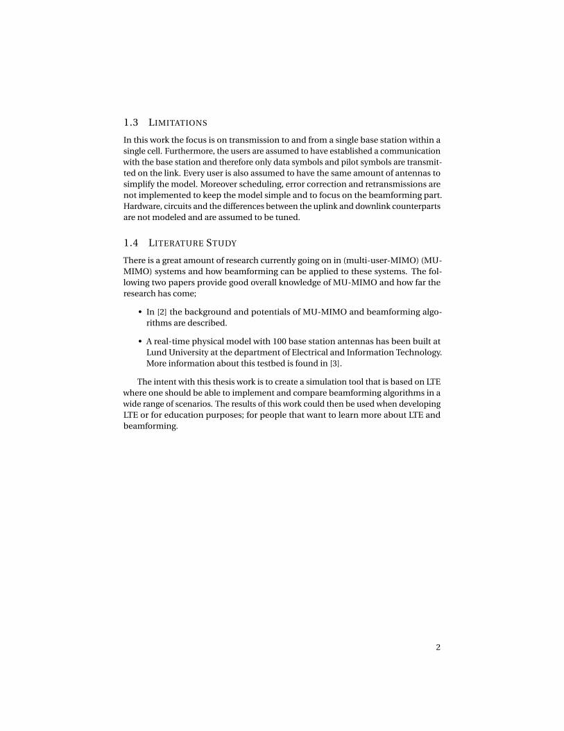
1.3 LIMITATIONS
In this work the focus is on transmission to and from a single base station within asingle cell. Furthermore, the users are assumed to have established a communicationwith the base station and therefore only data symbols and pilot symbols are transmit-ted on the link. Every user is also assumed to have the same amount of antennas tosimplify the model. Moreover scheduling, error correction and retransmissions arenot implemented to keep the model simple and to focus on the beamforming part.Hardware, circuits and the differences between the uplink and downlink counterpartsare not modeled and are assumed to be tuned.
1.4 LITERATURE STUDY
There is a great amount of research currently going on in (multi-user-MIMO) (MU-MIMO) systems and how beamforming can be applied to these systems. The fol-lowing two papers provide good overall knowledge of MU-MIMO and how far theresearch has come;
• In [2] the background and potentials of MU-MIMO and beamforming algo-rithms are described.
• A real-time physical model with 100 base station antennas has been built atLund University at the department of Electrical and Information Technology.More information about this testbed is found in [3].
The intent with this thesis work is to create a simulation tool that is based on LTEwhere one should be able to implement and compare beamforming algorithms in awide range of scenarios. The results of this work could then be used when developingLTE or for education purposes; for people that want to learn more about LTE andbeamforming.
2

2 BACKGROUND
This section covers technical standards and basics of how LTE works to give the readera better understanding of LTE before heading into more advanced topics. Only theparts that the authors deem necessary for a good understanding of this thesis arementioned. The information mostly originates from 3rd Generation PartnershipProject (3GPP) [4] which is an organization that collects and unites information frommultiple telecommunications developers to form a standard. The books [5], [6] and[7] summarize and present information from 3GPP in a way that is easy to follow andthese are the main sources of general information in the study.
2.1 UPLINK AND DOWNLINK
Transmission from user equipment (UE) to the base station is called uplink andtransmission in the opposite direction is called downlink. The most notable differencebetween UL and DL is that they use different multiple-access techniques. Singlecarrier frequency division multiple access (SCFDMA) is used in the UL, which isgood for the UE since it uses less power [5] than orthogonal frequency divisionmultiple access (OFDMA) which is used in the DL. This is because in OFDMA thedata is carried by a single subcarrier while in SCFDMA the data is carried by widersubcarriers. Thus the Peak to Average Power Ratio (PAPR) is lower for SCFDMA whichmakes the power amplification prior to transmission more efficient. With thesemultiple access techniques multiple streams of data to multiple users can be codedsimultaneously in time.
There are two techniques to handle the DL and UL transmissions, namely fre-quency division duplex (FDD) and time division duplex (TDD). FDD is used to sendUL and DL frames simultaneously using two separate frequency bands which meansthat data can be transmitted and received at the same time, increasing throughput.Another benefit with FDD is that it is easier to synchronize the packages since thereare separate links for UL and DL. TDD on the other hand is just using one frequencyband and the frames are divided in time instead, which means that the same channelis used for UL and DL transmissions and depending on the current flow in the net-work different UL/DL frame schemes can be used. This requires more precision insynchronization. In this thesis work TDD is used since the UL and DL channels areassumed to be reciprocal and almost stationary over a certain period of time which isbeneficial for beamforming. More about beamforming is covered in Section 4.
There is a set of frequency bands that are assigned for LTE TDD and each of thesebands is divided into channels with bandwidths according to Table 1. It is in one ofthese channels that the Matlab model operates in and the signals that are transmittedon the channel are described in the next section.
Channel Bandwidth 1.4 MHz 3 MHz 5 MHz 10 MHz 15 MHz 20 MHzSubcarriers 72 180 300 600 900 1200Resource Blocks 6 15 25 50 75 100
Table 1: Subcarriers and resource blocks as a function of the channel bandwidth, [5].
3

2.2 LTE RESOURCES
The largest unit in an LTE transmission is called a radio frame and it has two dimen-sions; time and frequency. Along the time axis it lasts for 10 ms. This radio frame isdivided into 10 subframes which are 1ms each which in turn is divided into two slotsof 0.5 ms. There are 14 symbols in a subframe and 7 symbols in a slot. A symbol is thesmallest unit in time and more about them is mentioned in Section 2.3. The radioframe and its subcomponents is shown in Fig. 1.
The length of the frequency axis depends on the channel BW, which is divided intonumerous subcarriers which each has a width of 15 kHz. The number of subcarriersare therefore related to the BW and this relation is seen in Table 1.
1 subframe
1 symbol
BW
1 slot 1 slot
10ms radio frame
#0 #1 #2 #3 #4 #5 #6 #7 #8 #9
Figure 1: Illustration of a LTE radio frame and its subcomponents, [8].
If one multiplies the subcarrier frequency of 15 kHz with the number of subcar-riers specified from the BW shown in Table 1. One can see that the subcarriers willnot cover the entire BW, as the edges are left unused to act as a guard band to reduceinterference from neighbouring channels.
If the time and frequency axes are combined, a grid will arise which is comprisedof units called resource elements (RE) which occupy one subcarrier in frequency andone symbol in time. A larger grid containing 12 subcarriers and 7 symbols is calleda resource block (RB). In the current implementation of LTE, two time-consecutiveRBs, spanning 14 symbols is the smallest unit that can be transferred to one UE at atime. These blocks are assigned to each UE using a scheduler, however in this thesisscheduling is not used and each UE is assigned a static number of RBs. Fig. 2 showsan example of how a 1.4 MHz subframe with 72 subcarriers and 14 symbols couldlook like. Each color represents the allocation to one UE.
4

2 4 6 8 10 12 14
Symbols
10
20
30
40
50
60
70
Subcarr
iers
UE 1
UE 2
UE 3
UE 4
UE 5
UE 6
Figure 2: Six users in a 1.4 MHz bandwidth subframe.
2.3 TRANSMISSION OF USER DATA
The user data is transferred in two physical channels which are called physical uplinkshared channel (PUSCH) for UL transmissions and physical downlink shared channel(PDSCH) for DL transmissions [5][7]. The channels have a set of resource elementsallocated for data symbols, i.e. a set of indices in the time-frequency grid whichcontain the user data. The user data arrives as bits to the transmitter unit and iscalled a codeword (CW). The codeword can be further divided into either one or twostreams of codewords, CW1 and CW2 as shown in Fig. 3 Before these codewords aretransmitted from the physical antennas they are processed in a few steps. To keep themodel simple, the steps in Fig. 3 are used which include symbol modulation, layermapping, precoding, resource mapping and OFDMA or SCFDMA modulation. Ina real system one would also like to include error detection which includes Cyclicredundancy check (CRC) insertion, code-block segmentation, turbo encoding, ratematching, code-block concatenation and scrambling as presteps to the ones shownin the figure. As mentioned earlier, error detection is not included to keep the signalprocessing of the transmitter and receiver chains simpler.
5

CW1
CW2
Symbol
Modulation
Layer
Mapping
Precoding and
Resource Mapping
OFDMA/
SCFDMA
Figure 3: Transmitter chain [13].
Symbol modulation is the stage where the bits are converted from ones and zerosto a complex number. This is done by mapping a sequence of bits to a number inthe complex plane. By giving a certain sequence of bits a certain amplitude andphase all combination of bits can be coded in sequence. In this project, four typesof modulation techniques are used; QPSK, 16QAM, 64QAM and 256QAM whichrespectively maps 2, 4, 6 and 8 bits into a single symbol. Fig. 4 - Fig. 7 shows theresulting complex valued symbols after modulation with the four modulators. Asseen in the figures, the more bits that are coded into a symbol the smaller the distancebetween each symbol will be. This means that modulation of a higher order will bemore sensitive to noise compared to a modulation technique with a lower order.On the other hand, a higher order modulation technique will transfer more bitsduring the same time interval. Therefore the modulation should change with thechannel conditions for optimal transmission. Note that the constellation diagramsare normalized such that the average power of the signal is equal to one.
-0.5 0 0.5
Real part
-0.8
-0.6
-0.4
-0.2
0
0.2
0.4
0.6
Ima
gin
ary
pa
rt
Figure 4: Constellation diagram QPSK.
-1 -0.5 0 0.5 1
Real part
-1
-0.5
0
0.5
1
Ima
gin
ary
pa
rt
Figure 5: Constellation diagram 16QAM.
6

-1.5 -1 -0.5 0 0.5 1 1.5
Real part
-1.5
-1
-0.5
0
0.5
1
1.5Im
ag
ina
ry p
art
Figure 6: Constellation diagram 64QAM.
-1.5 -1 -0.5 0 0.5 1 1.5
Real part
-1.5
-1
-0.5
0
0.5
1
1.5
Ima
gin
ary
pa
rt
Figure 7: Constellation diagram 256QAM.
Layer mapping is done to assign each symbol in the stream of symbols to a specificlayer. Layers in this context means the number of shared resources that are transmit-ted to the same user, and each layer must thus have orthogonal reference signals tobe separated. Table 2 shows how the mapping depends on the number of codewordstreams and the number of layers used, x l ayer refers to a layer and d codewor d refers
to a codeword stream. M l ayers ymb is the number of symbols for a specified layer. In this
project two codewords are used when using more than one layer. The more layersthat are used, the more data is transferred at the same time. Similar to modulation,the system is more sensitive to noise if it transmits more layers because it is moredifficult to separate the layers. To have a system of full rank, which means that all thetransmitted layers are successfully demodulated at the receiver, the system needs tohave at least the same number of transmit and receiver antennas as the number oflayers used.
Number oflayers
Number ofcodewords
Codeword-to-layermapping
i = 0, .., M l ayers ymb −1
1 1 x(0)(i ) = d (0)(i ) M l ayers ymb = M 0
s ymb
2 2x(0)(i ) = d (0)(i )x(1)(i ) = d (1)(i )
M l ayers ymb = M 0
s ymb = M 1s ymb
3 2x(0)(i ) = d (0)(i )x(1)(i ) = d (1)(2i )x(2)(i ) = d (1)(2i +1)
M l ayers ymb = M 0
s ymb = M 1s ymb/2
4 2
x(0)(i ) = d (0)(2i )x(1)(i ) = d (0)(2i +1)x(2)(i ) = d (1)(2i )x(3)(i ) = d (1)(2i +1)
M l ayers ymb = M 0
s ymb/2 = M 1s ymb/2
Table 2: Codeword-to-layer mapping [9].
The next two stages of coding are to precode the symbols of the layers with a setof weights and then to combine the layers and map them to the physical antennas. Itis at this stage that beamforming is performed and each physical antenna will then
7

have its own weighted resource grid. More about the beamforming can be found inSection 4.
In the final step the grids are converted to a waveform using either OFDMAor SCFDMA for DL or UL transmissions respectively. Cyclic prefix insertion is animportant part here [5]. In essence it is used to decrease the impact of the signal takingmultiple paths with different delays. The effect of this delay spread is that signalsarrive at different times. This means that two symbols with different time-index canarrive at the same time and interfere, which is called inter-symbol interference (ISI).When the receiver then samples the signal and does a fast Fourier transform (FFT)on the signal, it will contain a mix of frequencies from different symbols. This is aproblem and to handle it a cyclic prefix is inserted to every symbol. The cyclic prefixitself is the last part of every symbol and the length depends on the type of prefix,normal or extended. A normal cyclic prefix will cover for delay spreads up to 1.5 kmor about 5 µs and an extended prefix can handle delay spreads up to 5-10 km which is16.7-33.3 µs. Thus all symbols that arrives within the delay spread, inside of the cyclicprefix, will be seen as the same symbol. The FFT computes the frequency contentof the signal and the frequency content will not change with delayed componentsof the same signal. The last step of the modulation itself is to use an inverse Fouriertransform (IFFT) on the complex-valued signals to translate them into the timedomain. The signals are then transmitted on the wireless channel which is covered inSection 3, before they are received by the receiver chain explained in the next section.
2.4 RECEPTION OF USER DATA
The reception of data includes steps that are the inverse of the ones involved in thetransmitter chain. Namely OFDMA- and SCFDMA-demodulation, layer demappingand symbol demodulation. Channel Estimation and Channel Equalization are alsoadded to the chain and are very crucial in wireless transmission. The receiver chainthat is used in the model in this thesis is shown in Fig. 8.
OFDMA/
SCFDMA
Symbol
DemodulationCW1
CW2
Layer
DemappingChannel
Estimation
Channel
Equalization
Figure 8: Receiver chain [13].
Channel estimation is needed because when signals are transmitted over a wire-less channel, they lose their initial characteristics because of path loss, interference,fading and noise. For further explanation of these phenomena, see Section 3. Becauseof this, the signal will have a new amplitude and phase at the receiver. To compensatefor this, known pilot symbols are placed at known indices in the resource grid and
8

more about pilot symbols is mentioned in Section 2.5. In this way the receiver can dochannel estimation by comparing the received symbols with the known symbols. Thesymbols are spread across the grid depending on what transmission mode is used,the number of layers used and also if it is UL or DL transmission.
The channel estimate is computed according to the steps in [14]. First the channelestimate for all reference symbols is found using least squares. Then averaging isdone on the estimated reference symbols with an averaging-window spanning bothtime and frequency domain to suppress the effect from noise. Interpolation is thenperformed between the pilot symbols to retrieve a channel estimate over the entiregrid. It is done by finding the best fit of a line between the estimated and averagedsymbols of each column in the grid. The line can for example be either linear orcubic. The unknown symbols are then found from the indices of the fitted line andall of the lines are put together to a grid. Virtual pilot symbols may also be insertedoutside of the grid to increase the performance of the interpolation at the grid edges.These virtual pilots are found from a grid that is formed from the cross product of theoriginal pilots closest to the virtual pilot that you wish to generate.
Channel equalization is used to retrieve the user data from the channel estimate.This is simply the inverse channel estimate multiplied with the received symbolsto remove the channel impact. There are two well known ways of doing this, zero-forcing (ZF) and minimum mean-squared error (MMSE). The difference between thetwo methods is that MMSE uses the channel noise estimate while the ZF does not.The effect of this is that MMSE gives an equal or better estimate compared to ZF overthe entire SNR range [10].
2.5 REFERENCE SIGNALS
This thesis is focusing on transmission mode (TM) 9 and multilayer transmissions andtherefore the UE specific reference signal is used, it is also known as the demodulationreference signal (DM-RS). DM-RS generation differs between UL and DL both insignal generation and in grid indices [9, sections 5.5 and 6.10.3]. The idea with theDM-RS signal is that both the transmitter and receiver should be able to generate thesame sequence based on a number of parameters and thus be able to estimate thechannel. Because both transmitter and receiver knows what the sequence shouldlook like, they can estimate how the channel has affected the signal. In the uplink, thesignal is generated from a Zadoff-Chu sequence, which has the good properties thatit has a constant amplitude and can be sequentially shifted for orthogonality betweencells [11]. Orthogonal cover codes (OCC)s are used to achieve orthogonality betweenlayers by multiplying them with one Zadoff-Chu sequence to get a sequence for eachlayer. Creating orthogonality in this way is referred to as code division multiplexing(CDM). The OCCs used in this thesis are
OCC(λ) = e iα(λ)L, L = [0,1,2, ...k]
α(λ) = (0 π −π/2 π/2
),
(1)
where OCC(λ) is the OCC for layer λ and with the phase shift α, the sequences willbe orthogonal to each other, i.e. the dot product between the sequences is equal
9

to zero [12]. The sequence length k depends on the number of subcarriers [15]. Toget a good estimate of the entire uplink channel BW for all UEs, the UE pilots aresequentially allocated in the grid [3]. The resulting combined pattern of six UEs ina 1.4MHz BW channel is shown in Fig. 9, symbol columns 4 and 11 are the pilotsymbols and the rest are user data. The data resources are shared among all UEs andthe base station will be able to find the symbol for each individual UE since it has thechannel estimate of the entire channel for each UE. When transmission is done inthe model, each UE just transmits its own pilot symbols and leaves the rest empty,the figure is just as a visual aid.
Symbols
2 4 6 8 10 12 14
Subcarr
iers
10
20
30
40
50
60
70
Data
UE1
UE2
UE3
UE4
UE5
UE6
Figure 9: User allocation for six users in a 1.4 MHz bandwidth UL subframe.
According to LTE terminology, the downlink transmission is done on port 7 to 14and the number of ports used is equal to the amount of layers to be transmitted [6].Orthogonality between layers is obtained by using a mixture of frequency divisionmultiplexing (FDM) and CDM [5]. FDM is done by transmitting on different subcarri-ers; Ports 7,8,11 and 13 are transmitting on the same indices and ports 9, 10, 12 and14 are shifted downwards with one subcarrier compared to these and thus FDM isobtained. Within these two groups of ports CDM is used to get orthogonal sequences.
10

3 WIRELESS CHANNEL
This section aims to describe all parts that comprise the channel model in as muchdetail as needed to piece together the complete model. Reasons for choosing themodels used in this work are brought up and possible alternatives are presented,which should serve as a starting point for finding possible flaws in the model andsubsequently improving upon it.
3.1 CHANNEL MODEL
3.1.1 FADING MODEL
The wireless channel between user and base station is typically modeled using twodifferent probability distributions, depending on whether the user has a direct line-of-sight to the base station or not. If there is a direct line-of-sight a Rician distributionis used to model the complex-valued filter coefficients used to represent the channeland if not, a Rayleigh distribution is used. Since one can generally not assume thereto be a line-of-sight between base station and UE, the distribution used to model thechannel is a Rayleigh distribution, which has the probability density function
pR (r ) = 2r
Ωe
−r 2Ω , r ≥ 0 where Ω= E(R2), (2)
R is the random variable r is the value for which the probability is evaluated andE(R2) is the variance of R. The Rayleigh distributed variables are generated usinga method that creates a sum of sinusoids with independent uniformly distributedphase and amplitude as well as a frequency shift factor. There are several knownmethods of generating these sinusoids and the one used in this thesis has been shownto exhibit good statistical properties and was presented in [16]. As opposed to othersimilar methods such as Jakes’, the sum of sinusoids is properly stochastic in its natureand different generated paths are mutually uncorrelated [16]. Another property ofthis method is that it is very easy to generate exactly as many samples as needed. Thesum of sinusoids method is outlined in (3). This method converges quickly to theRayleigh distribution, so the computational cost can be kept low with a value of Maround 10 [16].
X (t ) = Xc (t )+ j Xs (t )
Xc (t ) = 2pM
M∑n=1
cos(ψn)cos(ωd t cos(αn)+φ)
Xs (t ) = 2pM
M∑n=1
sin(ψn)cos(ωd t cos(αn)+φ)
with αn = 2πn −π+θ4M
, n = 1,2, ..., M
(3)
where M is the number of sinusoids to sum, ψn , φ and θ are uniformly distributedon [-π, π) ∀n, and ωn is the maximum Doppler frequency.
11

3.1.2 TIME CORRELATION
Since the user is usually moving, the channel will also change over time, usuallycausing the received signal strength to deteriorate at random intervals. This is be-cause the received signal is a sum of all the different reflections of the sent signalthat propagates via different paths provided by the environment. At some pointsthese reflected signals may interfere destructively, while at other points they boostthe signal strength. This phenomenon is called multipath fading. The rate at whichthe channel is expected to experience a change in amplitude corresponds to howfast the user is moving and is characterized by the Doppler spectrum related to thatvelocity. The Doppler spectrum causes a temporal correlation in the channel, causingsubsequent samples to be correlated. This is also modeled in the Rayleigh modelpresented by (3).
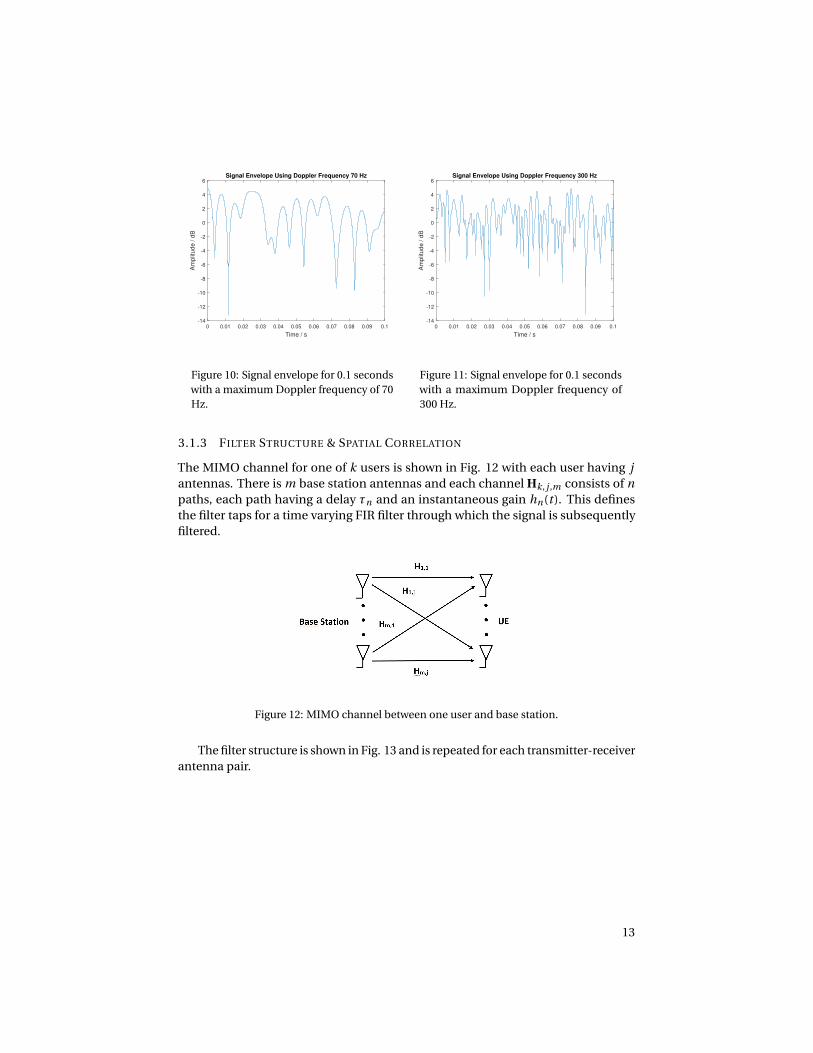
In the LTE standard [18], the number of most significant signal paths and theirrespective relative tap delays and losses are typically determined into three differ-ent scenarios; "Extended Pedestrian A" (EPA), "Extended Vehicular A" (EVA) and"Extended Typical Urban" (ETU) as shown in Table 3.
Profile Tap Delays (ns)EPA [0 30 70 90 110 190 410]EVA [0 30 150 310 370 710 1090 1730 2510]ETU [0 50 120 200 230 500 1600 2300 5000]
Profile Relative Power (dB)EPA [0.0 -1.0 -2.0 -3.0 -8.0 -17.2 -20.8]EVA [0.0 -1.5 -1.4 -3.6 -0.6 -9.1 -7.0 -12.0 -16.9]ETU [-1.0 -1.0 -1.0 0.0 0.0 0.0 -3.0 -5.0 -7.0]
Profile Max. Doppler Frequency (Hz)EPA 5EVA 5 or 70ETU 70 or 300
Table 3: Parameters for the different delay profiles specified in LTE [18].
For each of these paths, a complex-valued Rayleigh distributed sequence is gen-erated as outlined in Section 3.1.1. Each sequence then acts as the time-varyingenvelope with which the signal is filtered. The absolute value of envelopes withdifferent Doppler spectra is shown in Fig. 10 and 11.
12
0 0.01 0.02 0.03 0.04 0.05 0.06 0.07 0.08 0.09 0.1
Time / s
-14
-12
-10
-8
-6
-4
-2
0
2
4
6
Am
plit
ud
e /
dB
Signal Envelope Using Doppler Frequency 70 Hz
Figure 10: Signal envelope for 0.1 secondswith a maximum Doppler frequency of 70Hz.
0 0.01 0.02 0.03 0.04 0.05 0.06 0.07 0.08 0.09 0.1
Time / s
-14
-12
-10
-8
-6
-4
-2
0
2
4
6
Am
plit
ud
e /
dB
Signal Envelope Using Doppler Frequency 300 Hz
Figure 11: Signal envelope for 0.1 secondswith a maximum Doppler frequency of300 Hz.
3.1.3 FILTER STRUCTURE & SPATIAL CORRELATION
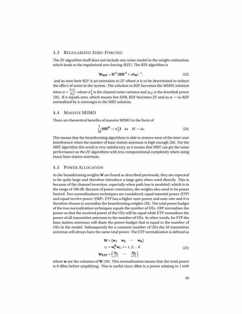
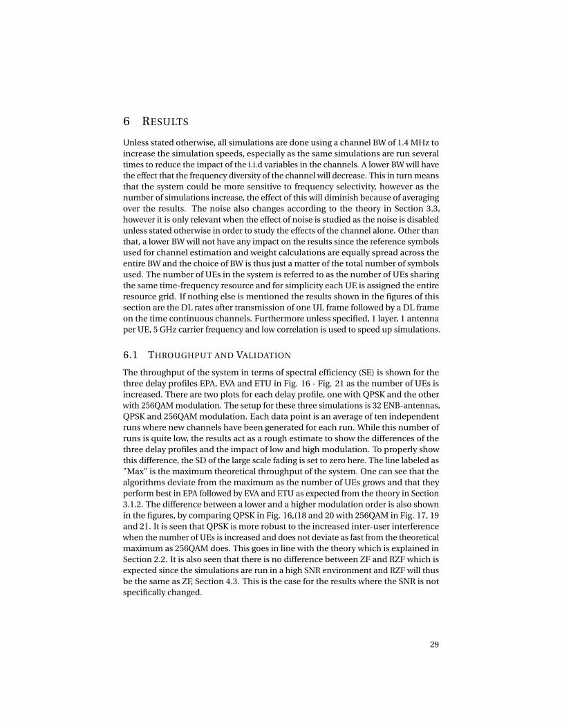
The MIMO channel for one of k users is shown in Fig. 12 with each user having jantennas. There is m base station antennas and each channel Hk, j ,m consists of npaths, each path having a delay τn and an instantaneous gain hn(t). This definesthe filter taps for a time varying FIR filter through which the signal is subsequentlyfiltered.
Figure 12: MIMO channel between one user and base station.
The filter structure is shown in Fig. 13 and is repeated for each transmitter-receiverantenna pair.
13
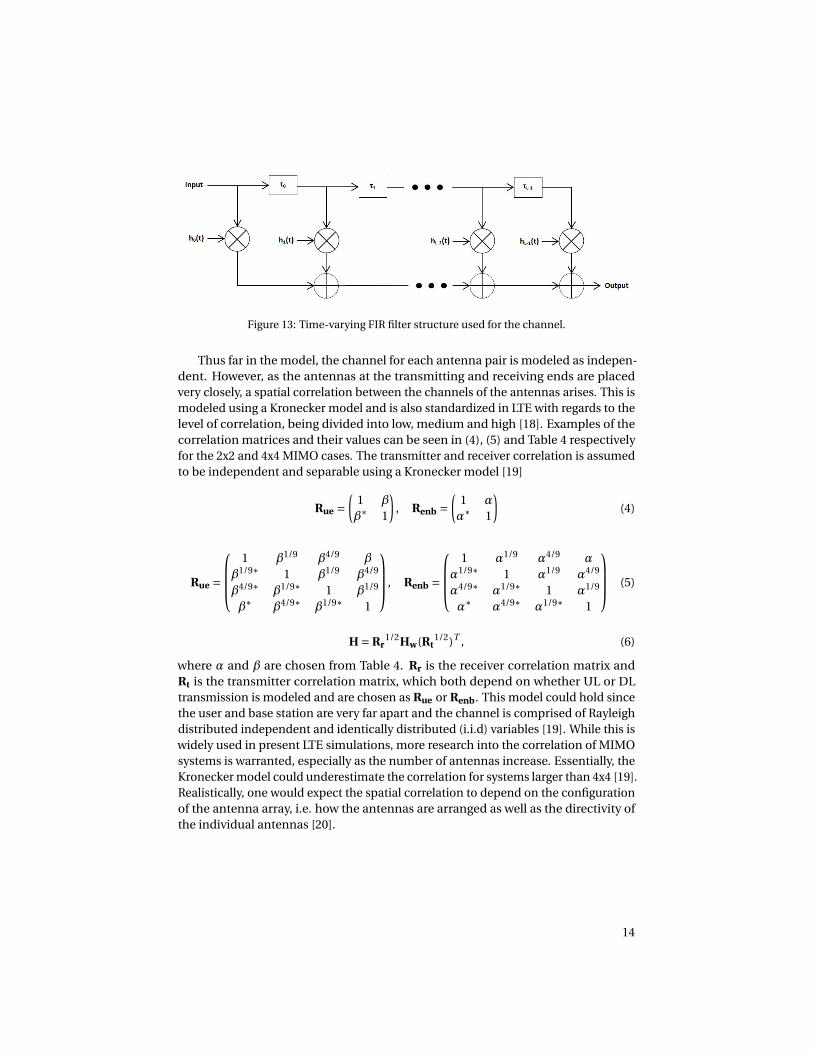
Figure 13: Time-varying FIR filter structure used for the channel.
Thus far in the model, the channel for each antenna pair is modeled as indepen-dent. However, as the antennas at the transmitting and receiving ends are placedvery closely, a spatial correlation between the channels of the antennas arises. This ismodeled using a Kronecker model and is also standardized in LTE with regards to thelevel of correlation, being divided into low, medium and high [18]. Examples of thecorrelation matrices and their values can be seen in (4), (5) and Table 4 respectivelyfor the 2x2 and 4x4 MIMO cases. The transmitter and receiver correlation is assumedto be independent and separable using a Kronecker model [19]
Rue =(
1 β
β∗ 1
), Renb =
(1 α
α∗ 1
)(4)
Rue =
1 β1/9 β4/9 β
β1/9∗ 1 β1/9 β4/9
β4/9∗ β1/9∗ 1 β1/9
β∗ β4/9∗ β1/9∗ 1
, Renb =
1 α1/9 α4/9 α
α1/9∗ 1 α1/9 α4/9
α4/9∗ α1/9∗ 1 α1/9
α∗ α4/9∗ α1/9∗ 1
(5)
H = Rr1/2Hw(Rt
1/2)T , (6)
where α and β are chosen from Table 4. Rr is the receiver correlation matrix andRt is the transmitter correlation matrix, which both depend on whether UL or DLtransmission is modeled and are chosen as Rue or Renb. This model could hold sincethe user and base station are very far apart and the channel is comprised of Rayleighdistributed independent and identically distributed (i.i.d) variables [19]. While this iswidely used in present LTE simulations, more research into the correlation of MIMOsystems is warranted, especially as the number of antennas increase. Essentially, theKronecker model could underestimate the correlation for systems larger than 4x4 [19].Realistically, one would expect the spatial correlation to depend on the configurationof the antenna array, i.e. how the antennas are arranged as well as the directivity ofthe individual antennas [20].
14

Correlation: Low Medium Highα: 0 0.3 0.9β: 0 0.9 0.9
Table 4: Correlation levels specified in LTE [18].
3.1.4 LARGE SCALE FADING
In addition to the fast-changing multipath fading determined by the Doppler shift,there is a large scale fading effect as well. This effect stems from the fact that whilemoving, a user can end up with a better or worse signal because of for examplebuildings, which are said to shadow the user. This fading is much slower-changingthan the multipath fading and follows a lognormal distribution [21]
pd f F (F ) = 20/l n(10)
FσFp
2πe− (20l og10(F )−µdB )2
2σ2F , (7)
where σF is the standard deviation (SD) of F and µdB is the mean of F in dB. Thestandard deviation of F is in the range of 4-10 dB [21] and this fading is centeredaround zero when generated. The large scale fading is then superimposed on thetime-varying filter taps for each user independently. Since this is an effect of the usermoving, the large scale fading will be correlated through time just as the multipathfading.
3.1.5 PATH LOSS
On top of the multipath fading and large scale fading effects, there is also a path lossattributed to the wireless channel. Assuming that the transmission is done in a noline-of-sight urban area the WINNER path loss model [22] is given by
PLdB = 23.5l og10(d)+57+23log10(fc
5), (8)
where fc is the carrier frequency in GHz (2 GHz < fc < 5 GHz) and d is the distancein meters between the receiver and transmitter (30 m < d < 5 km). Furthermore theheight of the base station and UEs are assumed to be 25 m and 1.5 m respectively. (8)in conjunction with the antenna gains is called the Friis transmission equation and isgiven by
Pr −Pt =Gt +Gr −PLdB . (9)
This represents the difference between received and transmitted power during trans-mission from one antenna to another, including antenna gains Gt and Gr .
3.2 UPLINK AND DOWNLINK RECIPROCITY
Since the duplexing mode used is TDD, the channel is highly correlated, if not con-stant between frames and particularly between UL and DL transmission. This is
15

because the same frequencies are used to transmit both in the UL and DL, and thusfrequency dependent effects of the channel are similar between UL and DL. The mostimportant element that changes is the fading, which is determined by the Dopplerfrequency and temporal correlation by advancing the channel one subframe in time.The other element that changes is the processing chain between transmitter andreceiver, importantly the amplifier used at the base station which is a high-poweramplifier contra the UE, which uses a low-power amplifier. Because they use differentamplifiers, the perceived channel will differ between UL and DL. This is currently notmodeled as explained in Section 1.3.
3.3 NOISE
The background noise used in the model is a simple well known thermal noise model[23] given by
vn2 = 4kB T R∆ f , (10)
where vn2 is the variance of the noise in Volts, kB is the Boltzmann constant, T is the
temperature in Kelvin, R is the resistance of the load in Ohm and∆ f is the bandwidthof the signal in Hz. The temperature is chosen as 300 K, "room temperature" andrealistically will only vary at most ± 30 K. The load resistance is chosen as the nominalimpedance for radio systems; 50 Ohm, and the bandwidth can be selected from thedifferent transmission standards within LTE [4] ranging from 1.4 MHz to 20 MHz asin Table 1.
3.4 COHERENCE TIME
As the channel changes over time, the beamforming will have to adapt to thesechanges in order to keep good performance. A measure of how quickly the channel ischanging is the coherence time [24]
Tc =√
9
16π f 2d
(11)
where fd is the maximum Doppler frequency. The coherence time tells us approxi-mately how long the channel will be time-invariant. This can be used to approximatehow long the beamforming weights will be valid for.
16

4 DOWNLINK BEAMFORMING
This section starts by describing some basics with beamforming and how it worksfrom a physical point of view and then continues with beamforming algorithms andhow they are implemented in the LTE model.
When two waves propagate in free space it is known from basic physics [25] thatthey interfere with each other if they are at the same position at the same time. If thishappens the amplitudes of the two waves are summed up and the interference canbe constructive, destructive or something in between. It is considered constructivewhen the waves have the same phase and the amplitude will then become higherthan that of one single wave. Conversely, destructive interference happens when thewaves are phase-shifted such that the total amplitude of the two waves becomes lessthan that of a single wave. Interference is used in practice by building an antennaarray with many antennas and transmit phase-shifted versions of the same signalfrom each antenna in the array. The total beam of all antennas will then interfereconstructively in some directions and destructively in others. If information aboutthe channel between the UEs and base station is known, the beamforming weightfor each antenna can be found such that the total beam can be steered towards theUEs. There are many ways of doing this, but in this thesis the focus will be on knownlinear precoding techniques that either maximizes the signal to noise ratio (SNR) orthe signal to interference and noise ratio (SINR) at each user in the system as in
Y = HDLWX+n, (12)
where W is the beamforming weighting matrix, X is the signals from all users, n is i.i.dGaussian noise, Y is a matrix with users and HDL is the downlink channel matrix withthe instantaneous gain and delay from each multipath between the K single antennausers and the M base station antennas. This channel matrix is further defined as
HDL =
hDL1,1(s) · · · hDL1,M (s)...
. . ....
hDLK ,1(s) · · · hDLK ,M (s)
. (13)
Each element hDL(s) in HDL is the instantaneous downlink channel amplitude andphase for the symbol located at index s in the resource grid as in
hDL(s) =
hDL 1,1 · · · hDL 1,14...
. . ....
hDL 1200,1 · · · hDL 1200,14
, (14)
where s = [s1, s2] and s1 = 1, 2, ... 1200 , s2 = 1, 2, ... 14 for a 20MHz BW channel with1200 subcarriers and 14 symbols. The idea is to loop through all symbols and findthe beamforming weight W for one symbol index at a time and then to weight this
17

symbol from all users X(s) to all antennas A(s) using A1(s)...
AM (s)
=
W1,1(s) · · · W1,K (s)...
. . ....
WM ,1(s) · · · WM ,K (s)
X1(s)
...XK(s)
, (15)
where X(s) and A(s) is the same size as one resource grid and thus has the same sizeas hDL(s). The weighted signals from all UEs are then transmitted over the channelaccording to Y1(s)
...YK (s)
=
hDL1,1(s) · · · hDL1,M (s)...
. . ....
hDLK ,1(s) · · · hDLK ,M (s)
A1(s)
...AM (s)
(16)
Multiple layers can be sent to each UE if the UEs are equipped with one antennafor each layer, resulting in a total of N antennas and layers. By introducing this intothe equations, (15) and (16) are extended to (17) and (18) respectively as
A1(s).........
AM (s)
=
W1,1,1(s) · · · W1,1,N (s) · · · W1,K ,1(s) · · · W1,K ,N (s)...
. . ....
. . ....
. . ....
WM ,1,1(s) · · · WM ,1,N (s) · · · WM ,K ,1(s) · · · WM ,K ,N (s)
X1,1(s)...
X1,N (s)...
XK ,1(s)...
XK ,N (s)
(17)
Y1,1(s)...
Y1,N (s)...
YK ,1(s)...
YK ,N (s)
=
hDL1,1,1(s) · · · hDL1,1,M (s)...
. . ....
hDL1,N ,1(s) · · · hDL1,N ,M (s)...
. . ....
hDLK ,1,1(s) · · · hDLK ,1,M (s)...
. . ....
hDLK ,N ,1(s) · · · hDLK ,N ,M (s)
A1(s).........
AM (s)
(18)
Three known beamforming algorithms are used in this work to find the beam-forming weights W and these algorithms are described in the next three subsections.To transmit in the opposite direction, the rows and columns of the channel matrixmust be swapped to keep the same channel between receiver and transmitter. Thus
18

the algorithms uses the transpose of the uplink channel estimate to produce thedownlink channel estimate, which we refer to as
H =
hUL1,1(s) · · · hULM ,1(s)...
. . ....
hUL1,K (s) · · · hULM ,K (s)
T
(19)
where hUL(s) is the uplink channel estimate for each symbol s and has the same sizeas hDL(s) in (14).
4.1 MAXIMUM RATIO TRANSMISSION
As explained in [26], maximum ratio transmission (MRT) maximizes the SNR for eachuser. This algorithm has very low complexity as it is the Hermitian of the channel H,i.e. the conjugate-transpose of the channel and the beamforming weights are chosenaccording to
WMRT = HH. (20)
The cost of the low complexity is that the system is sensitive to inter-user interfer-ence which increases with the number of UEs in the system. The interference alsooriginates from channel correlation and white noise and this reduces the orthogonal-ity of the system which in turn leads to a lower throughput.
4.2 ZERO-FORCING
The well known ZF algorithm maximizes the signal to interference and noise ratio(SINR) of the system and it has been explained in previous work [26], [27] and [28].Some good properties of this algorithm are that it cancels interference between usersand is straight forward to implement since the beamforming weights are the pseudo-inverse of the channel. A drawback with this algorithm compared to MRT is theincreased complexity due to inversion calculations. One condition for the ZF to be awell defined problem is that the number of base station antennas must be at least thetotal number of all user antennas as stated in
M Ê K N , (21)
where, once more, M is the number of base station antennas, K the number ofUEs and N the number of antennas per UE. The beamforming weights W are thencalculated as the pseudo-inverse of the channel matrix H;
WZF = HH (HHH )−1. (22)
19
4.3 REGULARIZED ZERO-FORCING
The ZF algorithm itself does not include any noise model in the weight estimation,which leads to the regularized zero forcing (RZF). The RZF algorithm is
WRZF = HH (HHH +αIM)−1, (23)
and as seen here RZF is an extension to ZF where α is to be determined to reducethe effect of noise in the system. The solution to RZF becomes the MMSE solution
when α= Kσ2h
pdl, where σ2
h is the channel noise variance and pdl is the downlink power[26]. If α equals zero, which means low SNR, RZF becomes ZF and as α→∞ RZFnormalized by α converges to the MRT solution.
4.4 MASSIVE MIMO
There are theoretical benefits of massive MIMO in the form of
1
MHHH →σ2
h I as M →∞. (24)
This means that the beamforming algorithms is able to remove most of the inter-userinterference when the number of base station antennas is high enough [26]. For theMRT algorithm this result is very satisfactory, as it means that MRT can get the sameperformance as the ZF algorithms with less computational complexity when usingmany base station antennas.
4.5 POWER ALLOCATION
As the beamforming weights W are found as described previously, they are expectedto be quite large and therefore introduce a large gain when used directly. This isbecause of the channel inversion, especially when path loss is modeled, which is inthe range of 100 dB. Because of power constraints, the weights also need to be powerlimited. Two normalizations techniques are considered; equal transmit power (ETP)and equal receive power (ERP). ETP has a higher sum-power and sum-rate and it istherefore chosen to normalize the beamforming weights [29]. The total power budgetof the two normalization techniques equals the number of UEs. ERP normalizes thepower so that the received power of the UEs will be equal while ETP normalizes thepower of all transmitter antennas to the number of UEs. In other words, for ETP thebase station antennas will share the power budget that is equal to the number ofUEs in the model. Subsequently for a constant number of UEs the M transmitterantennas will always have the same total power. The ETP normalization is defined as
W = (w1 w2 · · · wK
)ci = wH
i wi, i = 1, 2, .. K
WETP =(
w1pc1
· · · wKpcK
) (25)
where w are the columns of W [29]. This normalization means that the total poweris 0 dBm before amplifying. This is useful since dBm is a power relating to 1 mW
20

and by relating the signal power to a physical quantity, the signal can be amplifiedsuch that all the available power is fully utilized. This means a total power acrossall base station antennas of 46 dBm and a total of 23 dBm for each UE [18]. Thepower allocated to each antenna could then be decided through different allocationschemes. One such scheme is to allocate different users different power, which canbe further specified whether the goal is equal throughput to all users, or maximizingtotal throughput. In the present model however, a more heuristic scheme of dividingthe power equally among the base station antennas is used.
21


5 MODELING USING LTE SYSTEM TOOLBOX IN MATLAB
5.1 INTERFACE
The Matlab model is constructed as a graphical user interface (GUI) to make testingand comparison with different setups easier due to all the parameters that are in-cluded in an LTE model. Even though the model is made to be as simple as possibleand yet have the necessary functions, there are a lot of user parameters that can beset as shown in Fig. 14. On the left hand side of the GUI one can see all parametersthat can be changed in the model and they are divided into two groups; channel-and link parameters. The name of the parameter reveals most of its functionality butmore precisely how they affect the underlying model is described in the followingsections. Other than the user parameters there are also plots that show results fromsimulations and buttons for channel creation and frame transmission.
Figure 14: GUI.
The following list contains a summary of what the model supports to get anoverview of its functionality;
• TDD transmission in UL and DL
• Scalable in terms of number of base station antennas and UEs
• Transmit 1-4 Layers to each UE
• LTE BWs of 1.4-20 MHz
• Four delay profiles; EPA, EVA, ETU and custom input
23

• Four modulation levels in DL; QPSK, 16QAM, 64QAM and 256QAM
• MRT, ZF and RZF beamforming
• Can transmit consecutive UL/DL frames on a time correlated channel
• Performance is presented in a constellation diagram and as bit error rate (BER)from frame to frame
5.1.1 CHANNEL SETUP
All parameters within this group basically have to do with the channel as stated inthe title. The "#ENB Antennas" setting is simply the number of base station antennasto be used in the simulation and they are plotted in the Spatial Layout plot togetherwith the number of UEs that are added from the add UE panel. The distances arein meters and the plot is there to remind the user of how many users he or she hasadded. The carrier frequency sets the spacing between the base station antennas andaffects the path loss in the model. The bandwidth chooses the amount of subcarriersthat are used according to Table 1 and under the button "Configure ENB" the lengthof the channel in time is decided as the total number of subframes. This is to ensurethat the frames are time correlated and continuous. Layers determine the number ofshared resources that should be transmitted to each UE and each UE should also beequipped with at least that number of antennas for a sufficient transmission. Finallythe delay profile is chosen as either EPA, EVA, ETU or as a custom made model. EPA isthe simplest model as it models a pedestrian and ETU is the most complex, modelinglong distances in urban terrain.
When all of the parameters are set, the channels are created by pressing the button"Generate Channel(s)". The channels are generated as described in Sections 3.1 and5.3, and the channels can also be cleared to the default settings by pressing "ClearChannel(s)". Worth mentioning is that the generated channels can be used multipletimes with different link setups. This is implemented since channel generation can bea time consuming part of the simulation when simulating a high BW with many usersand base station antennas. This way many different settings can be tested withouthaving to regenerate the channels.
5.1.2 LINK SETUP AND TRANSMISSION
We start from the top of the link setup with "Antenna Correlation". This is thecorrelation between the UE antennas and the correlation between the ENB antennas,and can be chosen as low, medium, or high according to Table 4. The next option is alist menu to choose between the implemented downlink beamforming algorithmswhich are described in Section 4. Further, the modulation level can be set for the ULand DL respectively and determines the amount of data to transmit as mentioned inSection 2.3. There is QPSK, 16QAM and 64QAM in both directions and there is also256QAM in the DL. The two next parameters "ENB Power" and "UE Power" decideshow much total power is available to the base station and UEs respectively duringtransmission.
24

Subframes are generated and transmitted with the buttons located in the bottomright of the GUI window. "Send Initial Frames" transmits one uplink frame to get anestimate of the channel and then it transmits one downlink frame that is weightedwith the beamforming weights found using the uplink estimate. The received down-link constellation at the UE will be shown in the right plot and if there are multipleUEs in the model the button "Switch UE" will toggle between the constellation dia-grams of the different UEs. The user can chose to send consecutive downlink framesto see how the performance of the beamforming algorithm changes with time with"Send Next DL Frame(s)". This can also be illustrated in the left plot; if the "DL BER"button is pressed a plot of the BER as a function of time for one UE will be shown. The"Switch UE" button will also toggle between the BER plots. If one wishes to return tothe spatial layout the button "Layout" can be used, and finally if one wishes to updatethe beamforming weights, the button "Send Next UL Frame and Update Estimate"will do as stated in the button text.
There is also a terminal that prints the SNR, BER and total transmitted bits in theUL, and for the DL it prints SNR, BER and total transmitted bits to each UE. This isdone for each beamforming algorithm and the information can be saved to a .txt filefor later comparison using the "Log to File" buttons.
5.2 UPLINK
The main task of the uplink in this model is to provide the base station with a channelestimate for each UE. To be able to reduce inter-user interference, the entire channelBW must be estimated to provide the beamforming algorithms with sufficient infor-mation. All uplink frames are built according to the scheme shown in Fig. 3. PUSCHdata symbols and DM-RS symbols are placed in the grid and the DM-RS symbolsare used for channel estimation as mentioned in Section 2.5. The PUSCH symbolsare used as a measure of how good the channel estimator is. The model also allowstransmission of multiple layers, when multiple layers are used the UEs will allocatethe same time-frequency resources in the grids and each grid will be transmitted on aseparate UE antenna. With the use of orthogonal pilots as explained in Section 2.5 thegrids will be orthogonal to each other and this will also be true for the UE antennas.Due to this orthogonality between the antennas, the estimator at the base station willbe able to estimate the link between all of the transmit and receive antenna pairs. Theuplink channel estimation is then saved and later used in downlink beamforming.After estimation the grid is equalized as mentioned in Section 2.4 and the BER for thePUSCH data for each individual user is calculated to get a performance measure ofthe estimator.
5.3 CHANNEL
When the "Generate Channel(s)" button is pressed, the channels between all ofthe antenna pairs are generated as described in Section 3.1, including the Rayleighmultipath fading using Doppler spectrum and time correlation. As the "Simulate"button is subsequently pressed, the filter taps are correlated using the Kronecker
25

model also described in Section 3.1.3 and the signal is then filtered using a time-varying FIR filter as shown in Fig. 13 with the previously generated filter taps. At thispoint, the path losses and antenna gains experienced by the signal are also added.Finally, the additive white Gaussian noise (AWGN) is added on top of the receivedsignal using the noise model described in Section 3.3. A block diagram of the programflow of the channel model in context during simulation is shown below in Fig. 15for the uplink. The central block here is the "LTEStep" block, which performs thechannel modeling and filtering. The same function "LTEStep" is also used in thesame manner in the downlink but in a different context.
26

Figure 15: The program flow of the channel model, "LTEStep" in context.
27

5.4 DOWNLINK
The base station creates the frames and resource grids that are transmitted to the UEsin the downlink according to the scheme shown in Fig. 3. The difference comparedto the uplink is that each UE is now assigned an entire grid which is filled withsymbols that is intended for that specific UE. All users share the same set of referencesymbols and if multiple layers are transmitted to the UEs they are separated withorthogonal reference symbols in a similar way as in the uplink. When all of the usergrids are generated, they are weighted to the antennas using one of the beamformingalgorithms in Section 4 before they are transmitted. Each UE uses the receiver chainas shown in Fig. 8 and the resulting constellation and BER after equalization is shownfor the UEs in the GUI. The equalization is done to correct the amplitude of thereceived signals to make sure that the symbol demodulator works as intended as thereceived symbols will be of low amplitude because of the experienced path-loss. Thisis important for modulation of higher order than QPSK since the amplitude in thefour quadrants impacts the resulting bits after demodulation.
28
6 RESULTS
Unless stated otherwise, all simulations are done using a channel BW of 1.4 MHz toincrease the simulation speeds, especially as the same simulations are run severaltimes to reduce the impact of the i.i.d variables in the channels. A lower BW will havethe effect that the frequency diversity of the channel will decrease. This in turn meansthat the system could be more sensitive to frequency selectivity, however as thenumber of simulations increase, the effect of this will diminish because of averagingover the results. The noise also changes according to the theory in Section 3.3,however it is only relevant when the effect of noise is studied as the noise is disabledunless stated otherwise in order to study the effects of the channel alone. Other thanthat, a lower BW will not have any impact on the results since the reference symbolsused for channel estimation and weight calculations are equally spread across theentire BW and the choice of BW is thus just a matter of the total number of symbolsused. The number of UEs in the system is referred to as the number of UEs sharingthe same time-frequency resource and for simplicity each UE is assigned the entireresource grid. If nothing else is mentioned the results shown in the figures of thissection are the DL rates after transmission of one UL frame followed by a DL frameon the time continuous channels. Furthermore unless specified, 1 layer, 1 antennaper UE, 5 GHz carrier frequency and low correlation is used to speed up simulations.
6.1 THROUGHPUT AND VALIDATION
The throughput of the system in terms of spectral efficiency (SE) is shown for thethree delay profiles EPA, EVA and ETU in Fig. 16 - Fig. 21 as the number of UEs isincreased. There are two plots for each delay profile, one with QPSK and the otherwith 256QAM modulation. The setup for these three simulations is 32 ENB-antennas,QPSK and 256QAM modulation. Each data point is an average of ten independentruns where new channels have been generated for each run. While this number ofruns is quite low, the results act as a rough estimate to show the differences of thethree delay profiles and the impact of low and high modulation. To properly showthis difference, the SD of the large scale fading is set to zero here. The line labeled as"Max" is the maximum theoretical throughput of the system. One can see that thealgorithms deviate from the maximum as the number of UEs grows and that theyperform best in EPA followed by EVA and ETU as expected from the theory in Section3.1.2. The difference between a lower and a higher modulation order is also shownin the figures, by comparing QPSK in Fig. 16,(18 and 20 with 256QAM in Fig. 17, 19and 21. It is seen that QPSK is more robust to the increased inter-user interferencewhen the number of UEs is increased and does not deviate as fast from the theoreticalmaximum as 256QAM does. This goes in line with the theory which is explained inSection 2.2. It is also seen that there is no difference between ZF and RZF which isexpected since the simulations are run in a high SNR environment and RZF will thusbe the same as ZF, Section 4.3. This is the case for the results where the SNR is notspecifically changed.
29

0 5 10 15 20 25 30 35
Number of UEs
0
5
10
15
20S
pe
ctr
al e
ffic
ien
cy /
bits/s
/Hz
ZF
RZF
MRT
Max
Figure 16: Spectral efficiency as a functionof UEs with QPSK and 32 ENB antennason an EPA channel.
0 5 10 15 20 25 30 35
Number of UEs
0
20
40
60
80
Sp
ectr
al e
ffic
ien
cy /
bits/s
/Hz
ZF
RZF
MRT
Max
Figure 17: Spectral efficiency as a functionof UEs with 256QAM and 32 ENB anten-nas on an EPA channel.
0 5 10 15 20 25 30 35
Number of UEs
0
5
10
15
20
Sp
ectr
al e
ffic
ien
cy /
bits/s
/Hz
ZF
RZF
MRT
Max
Figure 18: Spectral efficiency as a functionof UEs with QPSK and 32 ENB antennason an EVA channel.
0 5 10 15 20 25 30 35
Number of UEs
0
20
40
60
80
Sp
ectr
al e
ffic
ien
cy /
bits/s
/Hz
ZF
RZF
MRT
Max
Figure 19: Spectral efficiency as a functionof UEs with 256QAM and 32 ENB anten-nas on an EVA channel.
30

0 5 10 15 20 25 30 35
Number of UEs
0
5
10
15
20S
pe
ctr
al e
ffic
ien
cy /
bits/s
/Hz
ZF
RZF
MRT
Max
Figure 20: Spectral efficiency as a functionof UEs with QPSK and 32 ENB antennason an ETU channel.
0 5 10 15 20 25 30 35
Number of UEs
0
20
40
60
80
Sp
ectr
al e
ffic
ien
cy /
bits/s
/Hz
ZF
RZF
MRT
Max
Figure 21: Spectral efficiency as a functionof UEs with 256QAM and 32 ENB anten-nas on an ETU channel.
As the SE of the algorithms deviates from the maximum the error increases in thesystem. The six next figures Fig. 22 - Fig. 27 uses the same simulation setup as the sixprevious figures but instead of SE, the BER is plotted. The BER is a representationof the ratio between the inaccurately demodulated bits and the total number oftransmitted bits. A BER of 0 % is the case where all bits are transmitted correctly and aBER around 50 % is the same as guessing, i.e. the transmission is unsuccessful. Witha high BER, retransmissions are needed to provide the receiver with the necessaryinformation and this leads to delays and slower data rates in the system. Conversely,a low enough BER can be considered as zero in a real setting because of the errorcorrecting part in the system. As shown in Fig. 16 - Fig. 21 the SE is increased with thenumber of UEs but the same thing happens for the BER in Fig. 22 - Fig. 27. Thereforethe number of UEs sharing the same resources has to be chosen carefully to get agood trade-off between SE and BER to avoid retransmissions and achieve maximumrates in the system. As also shown in Fig. 22 - Fig. 27, the BER differs between thedelay profiles and an adaptive measure is needed to account for this. Note that thedata points that are not present in the BER plots indicates that there are no errors forthose points as the BER is plotted in a logarithmic scale.
31

0 5 10 15 20 25 30 35
Number of UEs
10-4
10-3
10-2
10-1
100
BE
R
ZF
RZF
MRT
Figure 22: BER as a function of UEs withQPSK and 32 ENB antennas on an EPAchannel.
0 5 10 15 20 25 30 35
Number of UEs
10-5
100
BE
R
ZF
RZF
MRT
Figure 23: BER as a function of UEs with256QAM and 32 ENB antennas on an EPAchannel.
0 5 10 15 20 25 30 35
Number of UEs
10-4
10-3
10-2
10-1
100
BE
R
ZF
RZF
MRT
Figure 24: BER as a function of UEs withQPSK and 32 ENB antennas on an EVAchannel.
0 5 10 15 20 25 30 35
Number of UEs
10-2
10-1
100
BE
R
ZF
RZF
MRT
Figure 25: BER as a function of UEs with256QAM and 32 ENB antennas on an EVAchannel.
32

0 5 10 15 20 25 30 35
Number of UEs
10-3
10-2
10-1
100
BE
R
ZF
RZF
MRT
Figure 26: BER as a function of UEs withQPSK and 32 ENB antennas on an ETUchannel.
0 5 10 15 20 25 30 35
Number of UEs
0.15
0.2
0.25
0.3
0.35
0.4
0.45
BE
R
ZF
RZF
MRT
Figure 27: BER as a function of UEs with256QAM and 32 ENB antennas on an ETUchannel.
6.2 PERFORMANCE IN MASSIVE MIMO
In the results of Fig. 28 - Fig. 30 it is shown how the SE changes with the numberof ENB-antennas for a constant number of UEs with the three delay profiles. Thesetup for these simulations is 4 UEs and QPSK modulation. It is seen that EPA andEVA reaches the maximum throughput at around 8 ENB-antennas for ZF and at 32ENB-antennas for MRT. In ETU all three algorithms have similar performance in thissetup and is almost at maximum throughput at 350 ENB-antennas. This matcheswith the result from (24), which says that the system performance increases with thenumber of base station antennas. To properly see the difference between the delayprofiles, large scale fading SD is again set to zero.
0 20 40 60 80 100 120 140
Number of ENB antennas
0
0.5
1
1.5
2
2.5
Sp
ectr
al e
ffic
ien
cy /
bits/s
/Hz
ZF
RZF
MRT
Figure 28: Spectral efficiency for 4 UEswith QPSK on an EPA channel as the num-ber of ENB antennas grows.
0 20 40 60 80 100 120 140
Number of ENB antennas
0
0.5
1
1.5
2
2.5
Sp
ectr
al e
ffic
ien
cy /
bits/s
/Hz
ZF
RZF
MRT
Figure 29: Spectral efficiency for 4 UEswith QPSK on an EVA channel as the num-ber of ENB antennas grows.
33

0 50 100 150 200 250 300 350
Number of ENB antennas
0
0.5
1
1.5
2
2.5
Sp
ectr
al e
ffic
ien
cy /
bits/s
/Hz
ZF
RZF
MRT
Figure 30: Spectral efficiency for 4 UEs withQPSK on an ETU channel as the number of ENBantennas grows.
6.3 MULTI-LAYER TRANSMISSION
The SE of the system will also depend on the number of layers that are being trans-mitted at the same time, as more layers increase the number of resource grids thatare transmitted. We should therefore expect almost a 1:1 ratio between the numberof layers and the SE. As the channel is slower and more antennas are being used, thenoise is kept at a minimum. This produces an almost linear increase in SE when thenumber of layers is increased as shown in Fig. 31 using 32 base station antennas andan EPA profile. Moreover, for Fig. 31 - Fig. 34 4 users are used at a small distance of[100 m, 100 m] in a two-dimensional grid with 1 antenna per user and QPSK modula-tion. The results are averaged over 50 independent runs. To properly evaluate theeffect of different channels and different number of antennas, the large scale fadingvariance is set to zero.
As the channel affects the signal more adversely, more layers become comparablymore inefficient as it is more difficult to separate them with the decreased accuracyof the beamforming as explained in Section 2.3. Fig. 32 also supports this. The samebehaviour is shown with 16 antennas in Fig. 33 and Fig. 34, but as the limit on thenumber of UEs and layers is met as shown in Fig. 34, the SE drastically worsens whenthe delay profiles are compared. Additionally, ZF in this case is outperformed byboth RZF and MRT because of the sensitivity of ZF to erroneous channel estimates[30]. Worth noting is that the BER for the worst case shown in Fig. 34 using 4 layersand 4 users is around 40 % even for the RZF and therefore not practical for realtransmissions. The BER could however be improved by increasing the number ofbase station antennas as shown in Fig. 28 - Fig. 30.
34

1 1.5 2 2.5 3 3.5 4
Layers
2
3
4
5
6
7
8
9
Sp
ectr
al E
ffic
ien
cy /
bits/s
/Hz
32 Base Station Antennas and EPA Delay
ZF
RZF
MRT
Figure 31: Spectral efficiency for 4 UEsusing QPSK and 32 antennas on an EPAchannel as the number of layers increases.
1 1.5 2 2.5 3 3.5 4
Layers
2
3
4
5
6
7
8
Sp
ectr
al E
ffic
ien
cy /
bits/s
/Hz
32 Base Station Antennas and EVA Delay
ZF
RZF
MRT
Figure 32: Spectral efficiency for 4 UEsusing QPSK and 32 antennas on an EVAchannel as the number of layers increases.
1 1.5 2 2.5 3 3.5 4
Layers
2
3
4
5
6
7
8
9
Sp
ectr
al E
ffic
ien
cy /
bits/s
/Hz
16 Base Station Antennas and EPA Delay
ZF
RZF
MRT
Figure 33: Spectral efficiency for 4 UEsusing QPSK and 16 antennas on an EPAchannel as the number of layers increases.
1 1.5 2 2.5 3 3.5 4
Layers
2
2.5
3
3.5
4
4.5
5
5.5
6
6.5
Sp
ectr
al E
ffic
ien
cy /
bits/s
/Hz
16 Base Station Antennas and EVA Delay
ZF
RZF
MRT
Figure 34: Spectral efficiency for 4 UEsusing QPSK and 16 antennas on an EVAchannel as the number of layers increases.
6.4 TRANSMISSION OF CONSECUTIVE FRAMES
To see for how long the beamforming weights are valid in the different delay profiles,a time-correlated channel spanning ten subframes is generated and one UL framefollowed by nine DL frames are transmitted on the channel. The following parametersare used in this setup; 32 ENB-antennas, 4 single antenna UEs, QPSK modulationand zero large scale fading SD to properly compare the delay profiles. Fig. 35 - Fig. 36shows how the BER changes with the number of consecutive DL frames in the delayprofiles EVA and ETU. For the EPA channel the beamforming weights give no errorsfor at least 9 subframes for all algorithms with this setup and is thus not plotted. Asexpected it is worse for the EVA profile as shown in Fig. 35 where the error is only zeroor close to zero for two subframes for the algorithms. With this setup the performance
35

is unsatisfactory for all the subframes in the ETU profile as shown in Fig. 36, thoughthe two first frames are better than the ones following. Due to the random nature ofthe channel and the fading as explained in Section 3.1.1, the BER can also periodicallyimprove as more DL frames are sent using the same estimates as shown in Fig. 36.Again, a missing data point means a BER of zero.
2 4 6 8
Subframe number
10-4
10-3
10-2
10-1
100
BE
R
ZF
RZF
MRT
Figure 35: The DL BER with QPSK on anEVA channel as a function of consecutiveDL frames.
2 4 6 8
Subframe number
0.15
0.2
0.25
0.3
0.35
0.4
BE
R
ZF
RZF
MRT
Figure 36: The DL BER with QPSK on anETU channel as a function of consecutiveDL frames.
As the two first subframes had the lowest BER in the EVA and ETU profiles, anothersimulation is done on a 15-subframe long channel where the weights are now updatedevery third subframe, i.e. looping the frame pattern of UL-DL-DL five times. Theresulting DL BER is shown in Fig. 37 and Fig. 38 for EVA and ETU respectively. As isexpected, the BER is significantly lower when the beamforming weights are updatedregularly to adapt to the changes of the time-varying channel.
2 4 6 8 10
Subframe number
10-4
10-3
10-2
10-1
BE
R
ZF
RZF
MRT
Figure 37: The DL BER using QPSK on anEVA channel as a function of subframeswhen the weights are updated every thirdsubframe.
2 4 6 8 10
Subframe number
0.15
0.2
0.25
0.3
BE
R
ZF
RZF
MRT
Figure 38: The DL BER using QPSK on anETU channel as a function of subframeswhen the weights are updated every thirdsubframe.
36

6.5 ALGORITHM COMPLEXITY
The computation times for the ZF and MRT algorithms as a function of the numberof UEs and ENB antennas are shown in Fig. 39. They are measured as an average of50 runs in Matlab during run time on a PC running Windows and are thus not exact.However the results show that the ZF-algorithms and MRT algorithms grow linearlyin complexity and that MRT is significantly faster than ZF. The average ratio betweenthe two algorithms gives that MRT is about 16.8 times faster than ZF, with the gapincreasing for larger systems.
0 2 4 6 8 10 12 14
Number of UEs and ENB antennas
0
0.005
0.01
0.015
Tim
e /
s
ZF
MRT
X: 7
Y: 0.000714
Figure 39: Computation time as the number ofUEs and ENB antenns grows.
6.6 EFFECTS OF CHANNEL DISCREPANCIES BETWEEN USERS
A phenomenon that arises when all users are sharing the same frequencies is thatusers with different channel conditions, for example different path loss, will expe-rience a higher BER than users with similar conditions. Most notably, this mostlyoccurs for the ZF algorithms as shown in the constellations diagrams in Fig. 40 - Fig.45. Illustrated below is also to what extent simply changing the distance of one of theusers affects the received constellations. The settings for these tests are a 20 MHzbandwidth, 32 base station antennas, EVA delay profile, 16QAM modulation andvarying distance. To show this effect, large scale fading SD is set to zero since it wouldotherwise affect the users independently and possibly nullify or amplify the resultsfrom these tests.
37

Figure 40: Received constellation of user1 in a system with two users close to thebase station.
Figure 41: Received constellation of user2 in a system with two users close to thebase station.
Figure 42: Received constellation of user1 in a system with one user close to thebase station and one further away.
Figure 43: Received constellation of user2 in a system with one user close to thebase station and one further away.
38
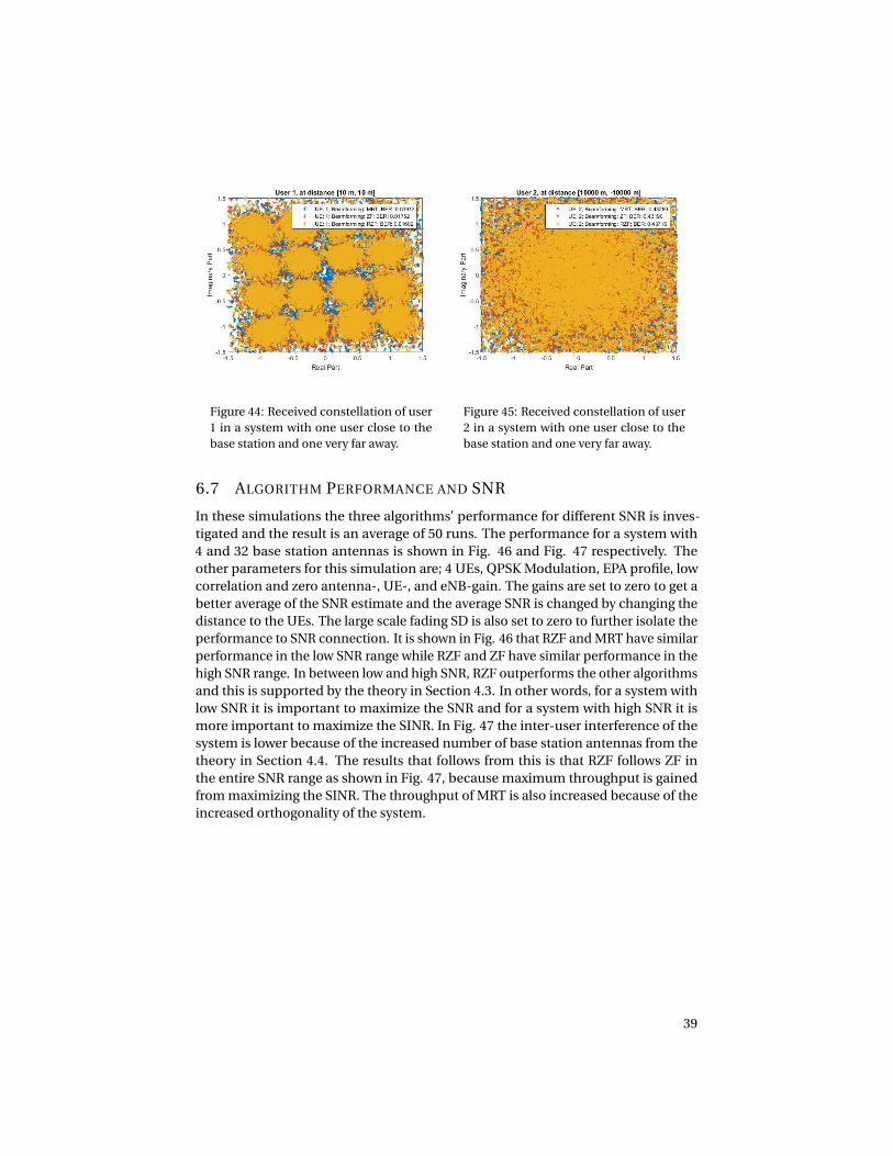
Figure 44: Received constellation of user1 in a system with one user close to thebase station and one very far away.
Figure 45: Received constellation of user2 in a system with one user close to thebase station and one very far away.
6.7 ALGORITHM PERFORMANCE AND SNR
In these simulations the three algorithms’ performance for different SNR is inves-tigated and the result is an average of 50 runs. The performance for a system with4 and 32 base station antennas is shown in Fig. 46 and Fig. 47 respectively. Theother parameters for this simulation are; 4 UEs, QPSK Modulation, EPA profile, lowcorrelation and zero antenna-, UE-, and eNB-gain. The gains are set to zero to get abetter average of the SNR estimate and the average SNR is changed by changing thedistance to the UEs. The large scale fading SD is also set to zero to further isolate theperformance to SNR connection. It is shown in Fig. 46 that RZF and MRT have similarperformance in the low SNR range while RZF and ZF have similar performance in thehigh SNR range. In between low and high SNR, RZF outperforms the other algorithmsand this is supported by the theory in Section 4.3. In other words, for a system withlow SNR it is important to maximize the SNR and for a system with high SNR it ismore important to maximize the SINR. In Fig. 47 the inter-user interference of thesystem is lower because of the increased number of base station antennas from thetheory in Section 4.4. The results that follows from this is that RZF follows ZF inthe entire SNR range as shown in Fig. 47, because maximum throughput is gainedfrom maximizing the SINR. The throughput of MRT is also increased because of theincreased orthogonality of the system.
39

-10 0 10 20 30
Average SNR / dB
1.2
1.4
1.6
1.8
2
2.2
2.4
2.6S
pe
ctr
al e
ffic
ien
cy /
bits/s
/Hz
ZF
RZF
MRT
Figure 46: 4 base station antennas.
-15 -10 -5 0 5 10 15 20
Average SNR / dB
1.4
1.6
1.8
2
2.2
2.4
2.6
Sp
ectr
al e
ffic
ien
cy /
bits/s
/Hz
ZF
RZF
MRT
Figure 47: 32 base station antennas.
6.8 ANTENNA CORRELATION
To demonstrate how the correlation parameter affects the throughput, simulationsare done with low, medium and high correlation which is specified in Section (3.1.3).The simulations are run with the following setup; 16 ENB Antennas, 2 layers, 2UE antennas, 2 UEs, EPA profile and 16QAM modulation. To see the effect of thecorrelation more separately, large scale fading SD is zero here. The throughput as thetotal number of correctly received bits is seen in Table 5, and the result is an averageof 50 runs. As expected the throughput is lower with more correlation because theinter-user interference is increased. It is also seen that the ZF algorithms handles theincreased interference better than MRT.
Low Medium High Max ThroughputZF 6816 6810.78 6747.52 6816RZF 6816 6811.14 6746.02 6816MRT 5867.44 4100.7 3957.64 6816
Table 5: Throughput for the three specified correlations.
6.9 MOBILITY
Given the layout of the pilot symbols and the length of one subframe as mentionedin Section 2.5 and the coherence time of the channel as in Section 3.4, the maximummobility the beamforming can handle can be calculated. The maximum updatingfrequency of the weights is when every second frame is an UL subframe, whichmeans every 14th symbol. Since the pilots are placed in symbol 4 and 11 of the ULsubframe, there are also 3 symbols at the end of the UL subframe during which thechannel can change. Therefore the weights need to be valid for at least 17 symbolsof approximately 71 µs each, which is approximately 1.2 ms in total. Using (11) inSection 3.4 and the Nyquist sampling theorem, the minimum sampling period is
40

given as
Tmi n =√
9
16π∗2 f 2d
(26)
where fd is the maximum Doppler frequency [31]. If the total time for the 17 symbols(1.2 ms) is inserted into (26), the approximate maximum Doppler frequency allowedfor a coherent channel is 174.85 Hz.
The simulations are run with 10 ENB antennas, 2 UEs and QPSK modulation overan average of 200 runs. Furthermore, zero large scale fading SD is used to properlyrelate the performance to the theory in Section 3.4. The SE is shown in Fig. 48 as theDoppler frequency is increased, and the throughput is at max for low frequenciesand starts to decrease after 100 Hz. Although the decrease is slow at first and onlypicks up at around 150 Hz.
Doppler frequency / Hz
60 80 100 120 140 160 180 200
Thro
ughput / bits/s
/Hz
1.16
1.17
1.18
1.19
1.2
1.21
1.22
ZF
Figure 48: SE plotted against Doppler frequency.
41

6.10 EFFECTS OF LARGE SCALE FADING
Thus far, the large scale fading has been inactivated to properly see the effects ofdifferent parameters. However as this effect can have a standard deviation of as muchas 4-10 dB independently per user as in Section 3.1.4, the performance could see anoticeable change when it is present. The spread of the large scale fading is shown inFig. 49 and Fig. 50 for a standard deviation of 4 dB and 10 dB respectively. The meanof the large scale fading is the path loss, which is set to -100 dB for this setup.
Figure 49: Spread of the large scale fadingaround a mean path loss of -100 dB and astandard deviation of 4 dB.
Figure 50: Spread of the large scale fadingaround a mean path loss of -100 dB and astandard deviation of 10 dB.
As can be seen, the effective attenuation of each user can be increased or de-creased by the large scale fading. Most importantly, the effect is independent foreach user meaning that users at the same distance do not necessarily experiencethe same SNR. This in combination with what is shown in Section 6.6 could giverise to slightly worse beamforming performance if the difference between users issignificant enough.
42

7 DISCUSSION
As mentioned in Section 3.1.3, the model used for correlating the channels might notbe inherently valid for large arrays [19]. Despite this, the Kronecker model is widelyused in the LTE standard [4] for this very purpose. The effect of this should presentitself once massive MIMO [2] becomes more prevalent and detailed models areneeded. Especially in beamforming situations where the antennas can be expected tobe placed fairly closely together which means that the correlation is higher. Howeverthe Kronecker model is simple to implement and a good starting point for the modelin this work, considering the goals set in Section 1.1.
Regarding the results in Section 6, one can see that almost every parameter is acompromise between robustness and throughput. Both more layers and more UEsrequire better channel estimates to reach full potential since the respective channelsneed to be separated to be properly decoded. As the channel changes, this initialestimate becomes a worse fit which means that the beamforming performance alsodeteriorates with time. To combat the deteriorating channel estimate, a new estimatecould be performed but at the cost of DL data rate since the system requires ULtransmissions to do so.
As shown in Section 6.6, having users with different channels may cause someusers to experience a worse BER than if they are modeled independently. This isan effect of the fact that all users currently use the entire resource grid. One wayto get around this would be to split the resource grid between users so that someusers exclusively use certain frequencies. Groups could also be made so that userswith similar channel conditions share the same frequencies. This also opens uppossibilities of different estimate updating frequencies for different groups, whichin turn increases the possible DL data rate for users with slower fading channels. Itthen follows that it could be of interest to expand the current model to include thepossibility of users with different channel conditions and as well as SNR.
Since the channel estimates need to be readily available to the transmitter forbeamforming, they need to be stored on the DSP. The storage needs will then dependon how many weights are needed to achieve good beamforming. For channelswhich are relatively flat in frequency, one weight per subcarrier may leave someweights redundant which could potentially at least halve the needed weights. Thisis completely dependent on the channel and could be a parameter varying withthe frequency selectivity of the channel. It could potentially also be a parameterindependent for each group of users, similar to how some users may need morefrequent channel estimates when the grid is split between the users as above.
When looking at the performance of the algorithms from the results in Section6 one can see that the ZF based algorithms performs better than MRT when thereare many users in the system transmitting on relatively flat channels. On the otherhand the complexity of MRT is much lower than the one of ZF and this is very crucialin LTE where transmissions are done every symbol, which is about 71 µs. Since thecurrent simulations are done in Matlab, little can be said about whether either ofthe algorithms are capable of computing within a single symbol. Another advantageof MRT in terms of complexity is that the computations can be parallellized anddone on each antenna element individually, since the user weighting to each antenna
43

is just using the specific antenna channel estimate. Furthermore the performancealso depends on the number of base station antennas and users sharing the sameresources, which is a design related topic. A complexity reduced ZF (CRZF) algorithmis proposed in [32] which starts from the MRT solution and cancels out the N worstinter-user interferers. As a theoretical result of this the complexity of the CRZF wasshown to be 2-7% of the original ZF while still keeping 90% of its performance. Thissounds very promising and should be further investigated.
Lastly, an idea for improving the current testing environment would be to includea surface plot in the layout plot, showing the signal strength at every point in space.This way one might see whether the algorithms provide correct beamforming throughanalysis of the signal strength at different points. It could also serve as an educationaltool, showing the differences of MRT and ZF in terms of interference cancelling.
7.1 CONCLUSION
In this work we have successfully built a model with the functionality stated inSection 5.1. The model also meets the requirements for investigating the statementsin Section 1.1 (Purpose & Aims) of this thesis. We have been able to find a way ofweighting the DL grids to the antennas and transmit the grids over a wireless channel.The algorithms MRT, ZF and RZF have been compared in different settings and it isseen that MRT is less complex than the ZF algorithms. The ZF algorithms on the otherhand are more robust to increased inter-user interference as many users transmitsin the same system. It is also seen that RZF outperforms MRT and ZF in the entireSNR range and we have been able to beamform up to four layers to each UE in thesystem. As a summary, the objectives have been met and the initial questions havebeen investigated and answered.
7.2 FUTURE WORK
If we were to continue work on this project, a first step would be to implement thecomplexity reduced zero-forcing algorithm and further study the complexity of all thealgorithms by implementing them in a real setting, where the computing times can beaccurately compared. Further improvements would be to find an adaptive algorithmthat calculates the number of UEs that should share the same resources as this isdependent on the channel conditions. Implementing adaptive weight updating bothin time and frequency would also be of interest. Finally improvements to the channelmodel would be investigated, specifically the spatial correlation for large antennaarrays and the inclusion of a Rician fading model to cover more simulation cases.
44
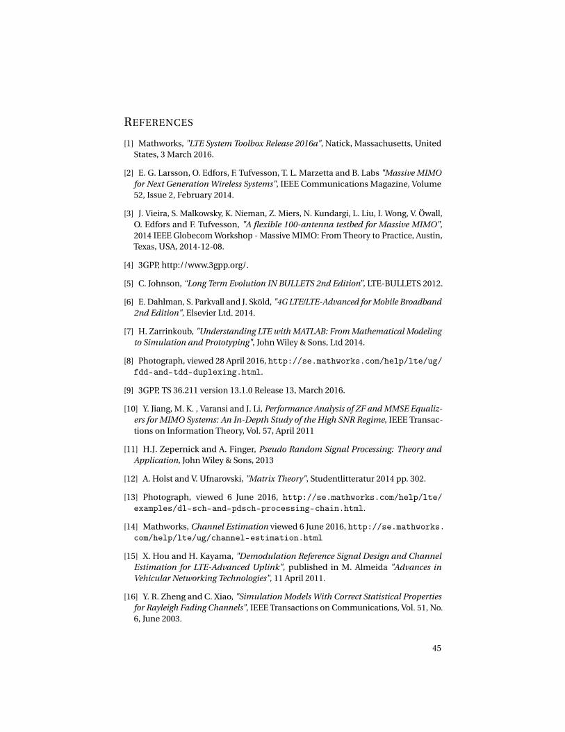
REFERENCES
[1] Mathworks, "LTE System Toolbox Release 2016a", Natick, Massachusetts, UnitedStates, 3 March 2016.
[2] E. G. Larsson, O. Edfors, F. Tufvesson, T. L. Marzetta and B. Labs "Massive MIMOfor Next Generation Wireless Systems", IEEE Communications Magazine, Volume52, Issue 2, February 2014.
[3] J. Vieira, S. Malkowsky, K. Nieman, Z. Miers, N. Kundargi, L. Liu, I. Wong, V. Öwall,O. Edfors and F. Tufvesson, "A flexible 100-antenna testbed for Massive MIMO",2014 IEEE Globecom Workshop - Massive MIMO: From Theory to Practice, Austin,Texas, USA, 2014-12-08.
[4] 3GPP, http://www.3gpp.org/.
[5] C. Johnson, “Long Term Evolution IN BULLETS 2nd Edition”, LTE-BULLETS 2012.
[6] E. Dahlman, S. Parkvall and J. Sköld, "4G LTE/LTE-Advanced for Mobile Broadband2nd Edition", Elsevier Ltd. 2014.
[7] H. Zarrinkoub, "Understanding LTE with MATLAB: From Mathematical Modelingto Simulation and Prototyping", John Wiley & Sons, Ltd 2014.
[8] Photograph, viewed 28 April 2016, http://se.mathworks.com/help/lte/ug/fdd-and-tdd-duplexing.html.
[9] 3GPP, TS 36.211 version 13.1.0 Release 13, March 2016.
[10] Y. Jiang, M. K. , Varansi and J. Li, Performance Analysis of ZF and MMSE Equaliz-ers for MIMO Systems: An In-Depth Study of the High SNR Regime, IEEE Transac-tions on Information Theory, Vol. 57, April 2011
[11] H.J. Zepernick and A. Finger, Pseudo Random Signal Processing: Theory andApplication, John Wiley & Sons, 2013
[12] A. Holst and V. Ufnarovski, "Matrix Theory", Studentlitteratur 2014 pp. 302.
[13] Photograph, viewed 6 June 2016, http://se.mathworks.com/help/lte/examples/dl-sch-and-pdsch-processing-chain.html.
[14] Mathworks, Channel Estimation viewed 6 June 2016, http://se.mathworks.com/help/lte/ug/channel-estimation.html
[15] X. Hou and H. Kayama, "Demodulation Reference Signal Design and ChannelEstimation for LTE-Advanced Uplink", published in M. Almeida "Advances inVehicular Networking Technologies", 11 April 2011.
[16] Y. R. Zheng and C. Xiao, "Simulation Models With Correct Statistical Propertiesfor Rayleigh Fading Channels", IEEE Transactions on Communications, Vol. 51, No.6, June 2003.
45

[17] D. J. Young and N. C. Beaulieu, "The Generation of Correlated Rayleigh RandomVariates by Inverse Discrete Fourier Transform", IEEE Transactions on Communica-tions, Vol. 48, No. 7, July 2000.
[18] 3GPP, TS 36.101 version 9.12.0 Release 9, July 2012.
[19] C. Oestges, "Validity of the Kronecker Model for MIMO Correlated Channels",IEEE 63rd Vehicular Technology Conference, Vol. 6, May 2006.
[20] DS. Shiu, G. J. Foschini, M. J. Gans and J. M. Kahn"Fading Correlation and ItsEffect on the Capacity of Multielement Antenna Systems", IEEE Transactions onCommunications, Vol. 48, No. 3, March 2000.
[21] A. F. Molisch, "Wireless Communications", John Wiley & Sons, 2005
[22] WINNER project, "IST-4-027756 WINNER II D 1.1.2 v1.2, WINNER II ChannelModels", https://www.ist-winner.org, 2006.
[23] H. Nyquist, "Thermal Agitation of Electric Charge in Conductors", Physical Re-view Vol. 32, July 1928.
[24] T. S. Rappaport, "Wireless Communications: Principles and Practice", 2nd Edi-tion, Prentice Hall, 2002
[25] Tipler P. A. and Mosca G. P., Physics for scientists and engineers. New York, W.H.Freeman 2003.
[26] X. Giao, Doctoral Thesis: "Massive MIMO in Real Propagation Environments",Lund University, January 2016.
[27] D. HN. Nguyen and T. Le-Ngoc, "MMSE precoding for multiuser MISO downlinktransmission with non-homogeneous user SNR conditions" EURASIP Journal onAdvances in Signal Processing, 6 June 2014.
[28] M. Sadek, A. Tarighat and A. H. Sayed, "A Leakage-Based Precoding Scheme forDownlink Multi-User MIMO Channels", IEEE Transactions on Wireless Communi-cations, Volume 6, 21 May 2007.
[29] M. Ghosh,"A Comparison of Normalizations for ZF Precoded MU-MIMO Systemsin Multipath Fading Channels", IEEE Wireless Communications Letters, Volume 2,2013.
[30] C. Wang, E. K. S. Au, R. D. Murch and V. K. N. Lau, "Closed-Form Outage Prob-ability and BER of MIMO Zero-Forcing Receiver in the Presence of Imperfect CSI",IEEE 7th Workshop on Signal Processing Advances in Wireless Communication,July 2006
[31] R. P. Jover, "LTE PHY Fundamentals", viewed 11 June 2016, http://www.ee.columbia.edu/~roger/LTE_PHY_fundamentals.pdf
[32] CS. Park, YS. Byun, A. M. Bokiye and YH. Lee, Complexity Reduced Zero-ForcingBeamforming in Massive MIMO Systems, Information Theory and ApplicationsWorkshop (ITA), 9-14 February 2014.
46