Adaptive Call Admission Control for QoS/Revenue Optimization in CDMA Cellular Networks

Christoph Lindemann, Marco Lohmann, and Axel Thümmler University of Dortmund

Department of Computer Science August-Schmidt-Str. 12

44227 Dortmund, Germany http://www4.cs.uni-dortmund.de/~Lindemann/

Abstract

In this paper, we show how online management of both quality of service (QoS) and provider revenue can be performed in CDMA cellular networks by adaptive control of system parameters to changing traffic conditions. The key contribution is the introduction of a novel call admission control and bandwidth degradation scheme for real-time traffic as well as the development of a Markov model for the admission controller. This Markov model incorporates important features of 3G cellular networks, such as CDMA intra- and inter-cell interference, different call priorities and soft handover. From the results of the Markov model the threshold for maximal call degradation is periodically adjusted according to the currently measured traffic in the radio access network. As a consequence, QoS and revenue measures can be optimized with respect to a predefined goal. To illustrate the effectiveness of the proposed QoS/revenue management approach, we present quantitative results for the Markov model and a comprehensive simulation study considering a half-day window of a daily usage pattern.

Keywords:

Network management & control,

admission control,

quality of service,

queueing/performance evaluation.

-2-

1 Introduction

The current evolution in mobile networks is primarily characterized by a transition from circuit-switched voice-oriented networks to integrated multi-service all IP networks. However, the support of multimedia services over wireless channels presents a number of technical challenges. One of the major challenges is to effectively utilize the scarce bandwidth in the radio access network. In CDMA cellular networks bandwidth is varying over time due to intra- and inter-cell interference, path-loss, fast fading, and shadowing [17]. Furthermore, user mobility can trigger rapid degradation in delivered quality of service (QoS) during a handover. These system characteristics result in time-varying QoS for mobile applications and, thus, the provision of different QoS classes and call priorities is desirable, e.g., as defined by the 3rd Generation Partnership Project (3GPP) [1].

For most multimedia applications, e.g., voice over IP or video conferencing, service can be degraded temporarily in case of congestion as long as it is still within the pre-defined range [4]. Thus, the system could free some radio capacity for new or handover calls by decreasing the QoS level of ongoing calls. Chou and Shin proposed an analytical model for a combined degradation and traffic restriction mechanisms [6]. Call degradation is for admission of more new and handover calls in the cell, and, hence, reduces the new call blocking and handover failure probability. However, the number of degraded calls is restricted by a fixed value that is not adjusted according to changing traffic load. In [16], Lataoui, Rachidi, Samuel, Gruhl, and Yan defined the components of a QoS management structure for packet switched 3rd generation mobile systems. They introduced the Seamless Service Descriptor as QoS parameter and specified an admission controller that utilizes this QoS parameter to allow degraded services at multiple levels according to a user specific profile. Das, Jayaram, Kakani, and Sen proposed a framework for QoS provisioning of multimedia services in 3G wireless access networks [7]. To support a differentiated treatment of real-time and non real-time traffic flows and to guarantee QoS demands, they developed a call admission controller that utilizes different schemes, i.e., channel reservation, bandwidth degradation, and bandwidth compaction. Service degradation with respect to revenue optimization was studied by Chlamtac, Das, and Záruba [4]. They proposed an admission control framework for optimal call mix selection to maximize the revenue earned by the service provider.

Several recent studies [5], [18], [19], [27] have been conducted concerning the forced-termination of calls due to handover failure. The dropping of a handover call is generally considered more serious than blocking of a new call. Therefore, a certain amount of bandwidth (also called guard channels) is exclusively reserved for handovers. This amount of bandwidth can be either fixed or adaptively controlled with respect to the current traffic load. In [20], we introduced an approach that determines the amount of bandwidth to be reserved for handover calls according to a look-up table, which was determined by extensive offline simulations. In [21], we extended this approach to general utility functions depending on

-3-

online monitored performance measures such as call blocking probability and handover failure probability. Furthermore, the improvement of both quality of service and provider revenue is considered for non real-time traffic. In order to improvement the dropping probability of soft handover calls, Ma, Han, and Trivedi considered a stochastic model for an admission controller in CDMA cellular networks that prioritizes soft handover calls using soft guard channels [22]. None of these previous papers investigates the prioritization of soft handover calls by applying a graceful degradation scheme that adapts to changing traffic load.

In this paper, we show how online management of both quality of service and provider revenue can be performed in CDMA cellular networks by adaptive control of system parameters to changing traffic conditions. As a main result, the approach is based on a novel call admission control and bandwidth degradation scheme for real-time traffic. We consider real-time calls with two priority levels: calls of high priority have a guaranteed bitrate whereas calls of low priority can be temporarily degraded to a lower bitrate in order to reduce forced termination of calls due to a handover failure. Opposed to previous work [6], [21], [22], we consider a graceful degradation of bandwidth in several steps. Furthermore, calls of low priority are degraded equally rather than picking out one call randomly for degradation. Clearly due to fairness reasons this approach should be preferred over a random choice of calls applied in [6]. A second contribution of this paper constitutes the development of a Markov model for the admission controller that incorporates important features of 3G cellular networks, such as CDMA intra- and inter-cell interference [17] and soft handover [12]. From the online quantitative analysis of the Markov model the threshold for maximal call degradation is periodically adjusted according to the currently measured traffic in the radio access network and a predefined optimization goal. We consider three different goals for the optimization of QoS and provider revenue: (i) minimizing call degradation subject to a hard constraint on handover failure probability, (ii) maximizing a QoS function, and (iii) maximizing a QoS/revenue function.

We present curves for measures of interest derived from the numerical steady state analysis of the Markov model. Besides the evaluation of the optimization goals, we compare the proposed degradation scheme with existing admission control policies based on adaptive guard channels [5], [27]. We show that overall utilization of cell capacity is higher with the degradation scheme, which can be considered as an "on demand" reservation of cell capacity whereas the guard channel scheme implements an "a-priori" reservation. Thus, the degradation scheme is the method of choice in future mobile networks, which support service degradation, since it can guarantee a certain handover failure probability and also high capacity utilization. The effectiveness of the proposed approach is illustrated by a comprehensive simulation study considering a half-day window of a daily usage pattern.

The paper is organized as follows. Section 2 presents the framework for QoS/revenue management and introduces the admission control and bandwidth degradation scheme. In

-4-

Section 3, we develop the Markov model of the admission controller and introduce three different goals for optimization. Results from quantitative analysis of the Markov model are presented in Section 4. Section 5 discusses implementation issues of the QoS/revenue management approach and presents a comprehensive simulation study. Finally, concluding remarks are given.

2 Framework for QoS/Revenue Management

2.1 General Description

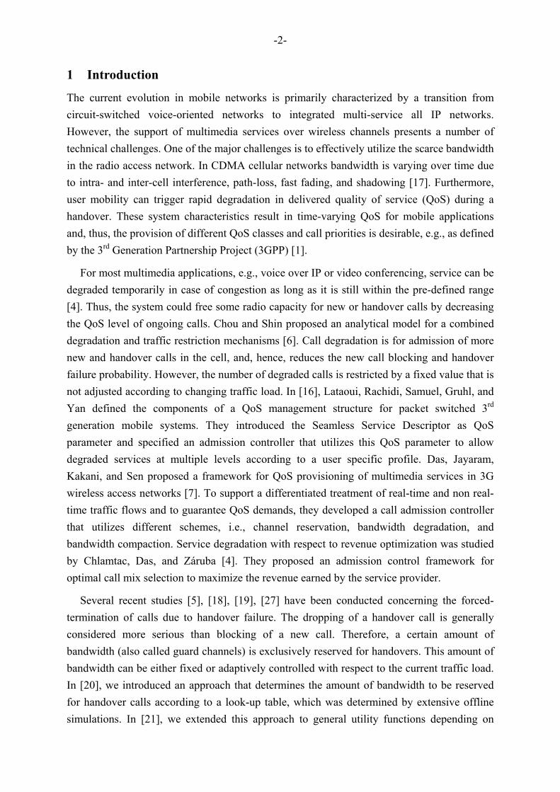
This section introduces the framework for the integrated management of both QoS and revenue in CDMA cellular networks. As illustrated in Figure 1, the framework is part of a base station controller (BSC) which is the primary controlling unit for a cluster of cells. The framework is subdivided into (1) the admission controller which decides whether to accept or reject a call request, (2) the online traffic measurement unit, and (3) the integrated QoS/revenue management unit which aims to determine the optimal setting of the admission controller in control periods of fixed duration. Thus, the proposed framework closes the loop between network operation and network control. In this paper, we focus on the optimization of just one adjustable parameter, i.e., the threshold for maximal bandwidth degradation, which is part of the admission controller introduced in the next section.

The optimization is based on the current traffic characteristics, called traffic pattern, determined by the online traffic measurement unit, a Markov model of the admission controller, and a predefined goal for QoS/revenue optimization. This Markov model

� � � � � � � � � � � � � � � �

� � � � � � �

� � � � �

� � � � � � �

� � � � � �

� � � � � � � � � � � � � � � � � � � � � � � � � � � � � � � � � � � � � � � � � � � � � � � � � � �

� � � � � � � � � � � � � � � � � � �

� � � � � � � � � � � �

� � � � � � � �

� � � � � � � � � � � �

� � � ! �

� � �

� � � � � � � � �

� � � � � � � � �

" � � � � � � � � � �

� � � � � � � � � � � � � �

Figure 1. Illustration of online QoS/revenue management

-5-

characterizes dependencies between the adjustable parameter of the admission controller and the traffic pattern. For different settings of the adjustable parameter, the evaluation of the Markov model yields a set of QoS and revenue measures crucial for optimization. Based on these QoS and revenue measures, the predefined goal for QoS/revenue optimization is evaluated. The parameter setting, which maximizes this goal is optimal for the current state of the radio access network, i.e., optimal for the current traffic pattern.

2.2 Admission Control Based on Bandwidth Degradation

This section describes the proposed admission control and bandwidth degradation scheme that is subject to be optimized according to the framework introduced in the previous section. Before a mobile user can start a new call, an admission controller decides to accept or reject the user's request. In general, this decision is based on the bandwidth requirements of the new call and the current network state, e.g., given by currently available bandwidth. Since the capacity of CDMA cellular systems is interference limited [17], the decision of the admission controller must be based on the interference in the considered cell (intra-cell interference) and the surrounding cells (other-cell interference). As introduced in the next section, a feasibility function determines whether a given system configuration is feasible in terms of CDMA cell capacity (see Eq. (8)). Intuitively, in a feasible system configuration the demands of all users in the system are satisfied. The admission controller performs a tradeoff between accepting a call request that may result in a QoS degradation of already admitted calls and rejecting a call request in order to guarantee ongoing calls a certain QoS. Furthermore, the admission controller prioritizes handover call requests over new call requests, since the dropping of a handover call is generally considered more serious than blocking of a new call.

Because of the scarcity of wireless cell capacity and the potentially large population of mobile users, it is desirable to offer preferential treatment to those who are willing to pay more for their service. This implies that the network will need to provide multiple service classes. Therefore, the proposed admission controller distinguishes two different call priorities, i.e., class-one calls correspond to calls of high priority and class-two calls are of lower priority. We abbreviate class-one calls with C1 calls and class-two calls with C2 calls, respectively. In order to prioritize handover call requests over new call requests as well as C1 calls over C2 calls, we consider an algorithm that temporally degrades the bandwidth reserved for C2 calls. Once the total required bandwidth exceeds the cell capacity, the system reduces the bandwidth currently assigned to C2 calls in order to admit more new C1 calls or handover calls, and hence reduces blocking probability of new C1 calls as well as the probability of handover failures. Suppose that without bandwidth degradation calls of class C1 and C2 require a bitrate of R kbps, respectively. The bandwidth degradation is performed stepwise in so called degradation steps of size δ. We assume that each C2 call could receive degraded

-6-

� �

� � � � � � � � � � � � � � � � � � � � � � � � � � �

� � � � � � � � � � � � � � � � � � � � � �

� � � � � � � � � � � � � � � � � � � � � � � � � � � � � � � � � � � � � � � � � � � � �

�

Figure 2. Bandwidth degradation scheme

service as long as this degraded service is within a tolerable range, i.e., a certain minimum bandwidth must be reserved for a C2. Therefore, the maximal number of degradation steps, denoted by mmax, is bounded by a degradation threshold θ, i.e., θ = mmax·δ (see Figure 2).

The admission controller considers the soft handover capability of CDMA cellular systems. Generally, CDMA systems enable handovers within a common radio access network (RAN), i.e., an intra-system handover, as well as handovers between two different RAN, i.e., inter-system handover. Throughout this paper, we consider a homogenous CDMA cellular network where neighboring cells use the same frequency band (intra-frequency) and do not take into consideration inter-system handover calls. Thus, the frequency has not to be changed at the time of a handover. Within an intra-system, intra-frequency CDMA system hard handovers can only occur if the handover is performed between two neighboring base stations with distinct BSC that are not connected due to radio network planning strategy or transmission reasons. Under these circumstances, intra-frequency hard handover is the only handover to support the seamless radio access.

According to [12], the vast majority of handovers are intra-system, intra-frequency soft handovers. Thus, we restrict our investigations to this kind of handovers. In fact, a mobile terminal near the cell boundary can maintain connectivity to an active set of more than one base station simultaneously. So when a mobile terminal with an ongoing call moves from one cell to another, the handover process happens in multiple steps. First the mobile notices the new cell, and the call will be carried on both cells. As the mobile continues to move, eventually the strength of the signal stemming from the cell the mobile is moving away from will drop to a point where it isn't useful any longer. Again, the mobile informs the cell system of this fact, and the system will drop the original cell. Because of this "make before break" transition this handover mechanism is called soft handover. In contrast, cellular systems based on FDMA and/or TDMA, such as GSM, employ the more traditional hard handover ("break before make"), where the mobile maintains connectivity to at most one base station at all times.

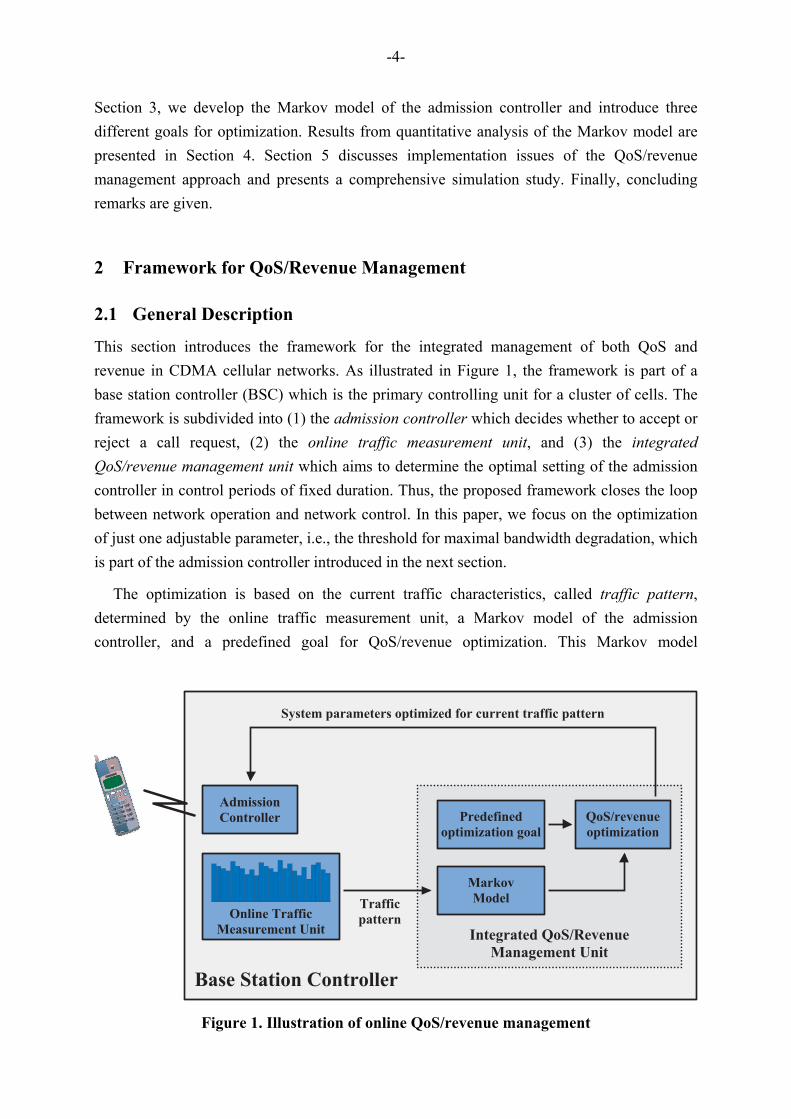
Figure 3 presents an activity diagram in Unified Modeling Language (UML) notation for decisions of the admission controller upon arrival of a new or soft handover call request. If the call request can be accommodated in the cell without exceeding the cell capacity the request is

-7-

� � � � � � � � � # �

� � � � � � � � � � � � �

� � � � � � � � � � � � � � � $ � �

# � � � � � � � � � � � % � � � �

& � � � � � � � � � � � � � �

� � � � � % � � � �

� # � � ! � $ # � � # � � � � � � � � ' �

' � � $ � � � # � � � � � � � � � � � � � � � �

� � � � � % � � � �

( � � � � � � � � � � )

( � � � � � � � � � )� � � � � � � �

� � % � � � �

& � � � � � � � � � � ' � � � �

� � � � � � � � � � � � � � � * � � * � � � % � � � � �

� � � � � � � � � � � � � $ � � +

� � � � � % � � � �

& � � � � � � � � � � ' � � � �

� � � � � � � � � � � � � � � * � � * � � � % � � � � � � �

� � � � � � � � � � � � � � # � � � � �

� � � � � % � � � �

( � � � ) ( � � � )

( � $ � � , � � � )

( � � � � # � � � � � � � � )( � $ � � + � � � )

( � � � � � � � � � - ) ( � � � � � � � - )

& � � � � � � � � , � � � � � �

� � � � � � � � � � � � � � � � �

& � � � � � � � � , � � � � � �

� � � - � � � � � � � � � � � � � � � �

& � � � � � � � � , � � � � � �

� � � � � � � � � � � � � � � � �

� � � � � � � $ � � +

� � � � � % � � � �

� � � � � � � � � � # � � � � �

� � � � � % � � � �

& � � � � � � � � � � ' � � * � ! * � �

% � � � � � � � � � � # � � � � � � � � �

� � � � � � � � � � # � � � � �

� � � � � � # � � � � � � % � � � �

� � � � � � � � � � � �

# � � � � � � � �

� � . � � � � � �

� � % � � � �

( � � � )

( ! � / � 0 )

& � � � � � � � � � � ' � � * � ! * � �

% � � � � � � � � � � # � � � � � � � � �

( � � � � # � � � � � � � � )

( � $ � � � )

� � . � � � � � �

� � % � � � �

( ! � 1 � 2 )( ! � 3 � 2 )

Figure 3. Activity diagram for admission controller: arrival of call request

granted. In case of insufficient bandwidth availability with respect to the feasibility function the admission controller distinguishes between C1 and C2 new calls and soft handover calls. New low priority call requests, i.e., new C2 calls, are rejected. In order to prioritize new C1 calls over C2 calls, the admission controller degrades C2 calls as long as the available bandwidth gets sufficient or a maximum of η·mmax degradation steps is reached. The parameter η, 0 ≤ η ≤ 1, specifies the extent of prioritizing C1 calls over C2 calls, i.e., η = 0 corresponds to no prioritization and η = 1 corresponds to maximal prioritization, respectively. If the available bandwidth is still insufficient, the new C1 call request must be rejected. Note that to accommodate a new C2 call the current number of degradation steps must not exceed

-8-

η·mmax steps. This is an important restriction to avoid prioritization of C2 calls in times of heavy degradation.

For soft handover calls the decisions are somewhat different. Independent of their priority, soft handover calls, can degrade other C2 calls to the maximum of mmax degradation steps. If the cell is still saturated, even with maximal degradation of C2 calls, the soft handover request may be queued in a handover queue with limited capacity K. Queued soft handover calls can (i) be accepted if sufficient bandwidth gets available, (ii) leave the cell, i.e., the mobile terminal moves to an adjacent cell or the call is completed, and (iii) be terminated due to timeout. Note that queued soft handover calls are still ongoing calls and thus, contribute to the intra-cell interference. In fact, queued soft handover calls lead to a cell overload with respect to the feasibility function. Therefore, we consider a timer for each queued soft handover call in order to bound this overload effect. Furthermore, the capacity of the handover queue should be reasonably small. In the case of a full handover queue, an arriving soft handover call request must be terminated to protect ongoing calls in the cell from further cell overload.

Figure 4 presents an UML activity diagram for the actions of the admission controller if the mobile terminal moves to an adjacent cell or a user completes the call. In terms of cell capacity a handover to an adjacent cell is similar to a call termination since no more resources are occupied in the cell (the call only contributes to the interference received from other cells). The admission controller checks whether the new available bandwidth is sufficient to accommodate a queued soft handover call. Recall that a queued soft handover call is only tolerated in the cell until a timer assigned to this call expires. In contrast, a regular accepted call is not restricted in his call duration. Therefore, it is desirable to admit a queued soft handover call in the cell if possible. If no more queued soft handover calls exist and bandwidth is still available, ongoing C2 calls are upgraded to a minimal number of required degradation steps with respect to the feasibility function.

� � � � � � � � � # �

� � � � � � � � � � � � �

� � � � � � � � � � � � � � �

� � � � � � # � � � � � � � � � � � � �

� � � � � � � � � , � � � � � � �

� � - � � � � � � � � ' � � ' � � $ � � � #( � � � � � � � � � � )

( � � � � � � � � � )

� # � � ! � $ # � � # � � � � � � � � ' �

' � � $ � � � # � � � � � � � � � � � � � � � �

% � � � � � � � � � � # � � � � � � � � �

( ! � 1 � 2 )

( ! � 3 � 2 )

� � � � �

% � � � � � � � � & � � � � � � � � � � ' � � * � ! * � �

% � � � � � � � � � � # � � � � � � � � �

Figure 4. Activity diagram of admission controller: call leaving the considered cell

-9-

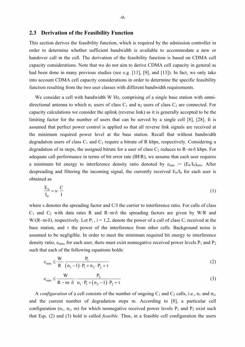
2.3 Derivation of the Feasibility Function

This section derives the feasibility function, which is required by the admission controller in order to determine whether sufficient bandwidth is available to accommodate a new or handover call in the cell. The derivation of the feasibility function is based on CDMA cell capacity considerations. Note that we do not aim to derive CDMA cell capacity in general as had been done in many previous studies (see e.g. [11], [9], and [13]). In fact, we only take into account CDMA cell capacity considerations in order to determine the specific feasibility function resulting from the two user classes with different bandwidth requirements.

We consider a cell with bandwidth W Hz, comprising of a single base station with omni-directional antenna to which n1 users of class C1 and n2 users of class C2 are connected. For capacity calculations we consider the uplink (reverse link) as it is generally accepted to be the limiting factor for the number of users that can be served by a single cell [8], [28]. It is assumed that perfect power control is applied so that all reverse link signals are received at the minimum required power level at the base station. Recall that without bandwidth degradation users of class C1 and C2 require a bitrate of R kbps, respectively. Considering a degradation of m steps, the assigned bitrate for a user of class C2 reduces to R−m·δ kbps. For adequate call performance in terms of bit error rate (BER), we assume that each user requires a minimum bit energy to interference density ratio denoted by emin := (Eb/I0)min. After despreading and filtering the incoming signal, the currently received Eb/I0 for each user is obtained as

b

0

E CsI I

= ⋅ (1)

where s denotes the spreading factor and C/I the carrier to interference ratio. For calls of class C1 and C2 with data rates R and R−m·δ the spreading factors are given by W/R and W/(R−m·δ), respectively. Let Pi , i = 1,2, denote the power of a call of class Ci received at the base station, and τ the power of the interference from other cells. Background noise is assumed to be negligible. In order to meet the minimum required bit energy to interference density ratio, emin, for each user, there must exist nonnegative received power levels P1 and P2 such that each of the following equations holds:

( )1

min1 1 2 2

PWeR n 1 P n P

≤ ⋅− ⋅ + ⋅ + τ

(2)

( )2

min1 1 2 2

PWeR m n P n 1 P

≤ ⋅− ⋅δ ⋅ + − ⋅ + τ

(3)

A configuration of a cell consists of the number of ongoing C1 and C2 calls, i.e., n1 and n2, and the current number of degradation steps m. According to [8], a particular cell configuration (n1, n2, m) for which nonnegative received power levels P1 and P2 exist such that Eqs. (2) and (3) hold is called feasible. Thus, in a feasible cell configuration the users

-10-

demands in terms of emin can be satisfied by choosing appropriate power levels P1 and P2. We assume that the relation of the received power levels P1 and P2 for C1 and C2 calls is directly proportional to the relation of the required bitrates, i.e.,

1

2

P RP R m

=− ⋅δ

. (4)

This is a fairly natural constraint that implies that increasing/decreasing the bitrate of C2 calls increases/decreases the received power at the base station in the same way. According to [8], we encapsulate the requirements of calls of class Ci, i=1,2, in the minimum signal to interference density ratio (SIDR) values, denoted by Γi:

1 minv R eΓ = ⋅ ⋅ (5)

( )2 minv R m eΓ = ⋅ − ⋅δ ⋅ , (6)

where v represents the activity factor of the call, e.g. v ≈ 0.4 for voice activity monitoring. In order to check whether a particular configuration is feasible, we need to determine τ, the received interference power from other cells. According to [26], [28], the received interference power from other cells can be computed by considering a relative other cell interference factor β. Let 1n and 2n be the average number of C1 and C2 calls per cell in a tier of cells surrounding the considered cell, respectively. Furthermore, let m be the average number of degradation steps in the surrounding cells. Applying Eq. (4), the interference power from other cells can be determined by:

( )R m1 1 2 1Rn P n P− ⋅δτ = β⋅ ⋅ + ⋅ ⋅ (7)

Inserting (4), (5), (6), and (7) into (2) and (3), defining ( )2 minv R m eΓ = ⋅ − ⋅δ ⋅ as the average requirements of C2 calls in the surrounding cells, and using some algebra, results in the following feasibility function:

( ) ( ) ( )1 1 2 2 1 1 2 21 2

feasible ,if n n 1 n n WF n ,n ,m

unfeasible ,else

Γ + Γ − + β⋅ Γ + Γ ≤=

(8)

3 Optimization of the Admission Controller

3.1 Markov Chain Analysis of the Admission Controller

The optimization of the admission control and bandwidth degradation scheme introduced in Section 2.2 is performed by means of a continuous time Markov chain (CTMC). In particular, the Markov chain is utilized to determine an optimal value for the degradation threshold θ (see Figure 2 for a definition of θ) with respect to a given traffic pattern and a predefined goal for optimization. This section shows how to efficiently analyze the Markov chain and to

-11-

derive QoS and revenue measures, which constitute the building blocks for the optimization goals, further specified in Section 3.2.

The Markov model considers the admission controller for one target cell. We assume that new call requests of class C1 and C2 arrive according to a spatially uniform Poisson process with arrival rate λn,1 and λn,2, respectively. Furthermore, soft handover requests from ongoing C1 and C2 calls arrive according to a Poisson process with rate λh,1 and λh,2, respectively. The amount of time that a mobile station with an ongoing call remains within the cell is called dwell time. With respect to the feasibility function (8), the dwell time is the time the call contributes to the intra-cell interference. Indeed, a soft handover to an adjacent cell can occur during the dwell time. Then the target cell and the corresponding adjacent cell serve the call simultaneously. If the call is still active after the dwell time, it leaves the cell to a neighboring cell without being in soft handover with the target cell anymore. The call duration is defined as the amount of time that the call will be active, assuming it completes without being forced to terminate due to handover failure. We assume the dwell time and the call duration to be exponentially distributed random variables with mean 1/µh and 1/µd, respectively. The overall rate of calls leaving the considered cell is denoted by µ = µd + µh. The reciprocal 1/µ is called cell residence time of a call. Recall that a queued soft handover call may be terminated by a timeout event. We assume the timeout event to be an exponentially distributed random variable with mean 1/µt. It should by noted that the assumption of exponentially distributed dwell times may be relaxed by including phase-type distributions in order to incorporate a slightly more realistic mobility process, while still allowing Markov chain analysis; however, the impact on the anticipated results and trends presented in this paper is expected to be insignificant, while obtaining the equilibrium distribution of the ensuing higher-dimensional Markov chain would be computationally more expensive.

A state of the model representing the target cell is determined by the number of active C1 and C2 calls, denoted by n1 and n2, respectively, the current number of degradation steps, denoted by m (0 ≤ m ≤ mmax), and the number of C1 and C2 calls waiting in the soft handover queue, denoted by k1 and k2 (k1+k2 ≤ K), respectively. Thus, the state of the queueing model can be expressed by a vector s = (n1, n2, m, k1, k2). The model dynamics are determined by the underlying continuous-time Markov chain that causes state transitions at random instants. State transitions correspond to different kinds of events that must be processed in the cell. The following kinds of events may occur:

(i) incoming new call request,

(ii) incoming soft handover call request,

(iii) call leaving the cell,

(iv) queued soft handover call leaving the cell.

-12-

Event type Condition Successor state Rate

New C1 call request k1+k2 = 0 ∧ ∃ m': m ≤ m' ≤ max(η·mmax, m) ∧ B(n1+1, n2, m', 0)

(n1+1, n2, m', k1, k2) λn,1

New C2 call request k1+k2 = 0 ∧ m ≤ η·mmax ∧ F(n1, n2+1, m) (n1, n2+1, m, k1, k2) λn,2

C1 call leaving cell

n1 > 0 ∧ ∃ m', k1', k2': 0 ≤ m' ≤ mmax ∧ 0 ≤ k1' ≤ k1 ∧ 0 ≤ k2' ≤ k2 ∧ Q(n1-1, n2, mmax, k1', k1, k2', k2) ∧ B(n1-1+k1', n2+k2', m', k1-k1'+k2-k2')

(n1-1+k1', n2+k2', m', k1-k1', k2-k2')

n1·µ

C2 call leaving cell

n2 > 0 ∧ ∃ m', k1', k2': 0 ≤ m' ≤ mmax ∧ 0 ≤ k1' ≤ k1 ∧ 0 ≤ k2' ≤ k2 ∧ Q(n1, n2- 1, mmax, k1', k1, k2', k2) ∧ B(n1+k1', n2-1+k2', m', k1-k1'+k2-k2')

(n1+k1', n2-1+k2', m', k1-k1', k2-k2')

n2·µ

∃ m': m ≤ m' ≤ mmax ∧ B(n1+1, n2, m', k1+k2)

(n1+1, n2, m', k1, k2) λh,1 Soft handover C1 call request k1+k2 < K ∧ ∀ m ≤ m' ≤ mmax:

¬B(n1+1, n2, m', k1+k2) (n1, n2, mmax, k1+1, k2) λh,1

∃ m': m ≤ m' ≤ mmax ∧ B(n1, n2+1, m', k1+k2)

(n1, n2+1, m', k1, k2) λh,2 Soft handover C2 call request k1+k2 < K ∧ ∀ m ≤ m' ≤ mmax:

¬B(n1, n2+1, m', k1+k2) (n1, n2, mmax, k1, k2+1) λh,2

Soft handover C1 call leaving queue

k1 > 0 ∧ ∃ m': 0 ≤ m' ≤ mmax ∧ B(n1, n2, m', k1-1+k2)

(n1, n2, m, k1-1, k2) k1·(µ+µt)

Soft handover C2 call leaving queue

k2 > 0 ∧ ∃ m': 0 ≤ m' ≤ mmax ∧ B(n1, n2, m', k1+k2-1)

(n1, n2, m, k1, k2-1) k2·(µ+µt)

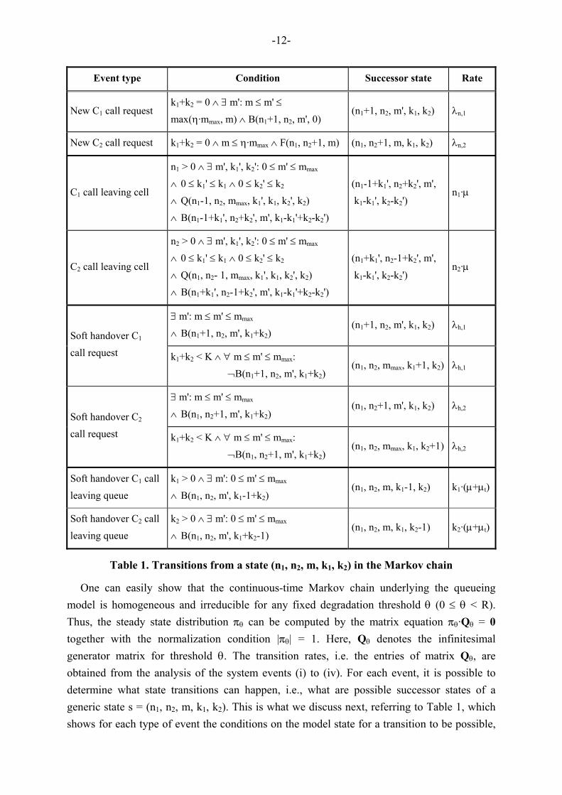
Table 1. Transitions from a state (n1, n2, m, k1, k2) in the Markov chain

One can easily show that the continuous-time Markov chain underlying the queueing model is homogeneous and irreducible for any fixed degradation threshold θ (0 ≤ θ < R). Thus, the steady state distribution πθ can be computed by the matrix equation πθ·Qθ = 0 together with the normalization condition |πθ| = 1. Here, Qθ denotes the infinitesimal generator matrix for threshold θ. The transition rates, i.e. the entries of matrix Qθ, are obtained from the analysis of the system events (i) to (iv). For each event, it is possible to determine what state transitions can happen, i.e., what are possible successor states of a generic state s = (n1, n2, m, k1, k2). This is what we discuss next, referring to Table 1, which shows for each type of event the conditions on the model state for a transition to be possible,

-13-

the rate associated with the transition, and the successor state. Note that different event types, e.g., a new call request and a soft handover request, can result in the same successor state. As a consequence, the overall rate for a transition to the considered successor state constitutes the sum of the individual rates, which must be stored in the generator matrix Qθ.

The actions of the admission controller introduced in Figures 3 and 4 are encapsulated in the enabling conditions presented in Table 1. For a proper representation, we define two Boolean functions B(n1,n2,m,k) and Q(n1,n2,m,k1',k1,k2',k2), where the former is responsible for bandwidth upgrade and bandwidth degradation of C2 calls and the latter accomplishes the admission of queued soft handover calls upon termination of a call in the target cell. Boolean function B(n1,n2,m,k) is 1 (i.e., true) if m is the minimum number of degradation steps required such that the cell configuration (n1,n2,m) is feasible with k queued soft handover calls. Boolean function Q(n1,n2,m,k1',k1,k2',k2) is 1 if k1' and k2' are the maximum number of queued C1 and C2 calls that can be regularly admitted such that the cell configuration (n1,n2,m) is feasible with k1 and k2 queued soft handover calls of class C1 and C2, respectively. Utilizing the feasibility function (8), B(·) and Q(·) are defined in Eqs. (9) and (10), respectively.

( )

( )( )( ) ( )( )

( )( )

1 2

1 2 1 21 2

max 1 2

1 , if k 0 m 0 F n , n , m

k 0 m 0 F n , n , m 1 F n , n , mB n , n , m, k

k 0 m m F n , n , m

0 , else

= ∧ = ∧ ∨ = ∧ > ∧ ¬ − ∧=

∨ > ∧ = ∧

(9)

( )

( ) ( )( )( )( )( )

1 1 2 1 1 2 2

1 1 2 1 11 2 1 1 2 2

1 1 2 2 2 2

1 , if F n k ,n ,m F n k ,n k ,m

F n k 1,n ,m k kQ n ,n ,m,k ,k ,k ,k

F n k ,n k 1,m k k

0 , else

′ ′ ′ + ∧ + +

′ ′∧ ¬ + + ∨ =′ ′ =

′ ′ ′∧ ¬ + + + ∨ =

(10)

As mentioned above, Table 1 shows for each type of event the conditions for state transitions. These conditions are formed by means of Boolean predicates, i.e., the Boolean functions B(·) and Q(·) and existential/universal quantifiers. The conjunction of Boolean functions and quantifiers guarantee that the successor state is unique and optimal with respect to the set of possible successor states. To illustrate this, consider a soft handover C1 call request and the condition: ∃ m': m ≤ m' ≤ mmax ∧ B(n1+1, n2, m', k1+k2) (see Table 1). The Boolean function B(·) is evaluated for each m' in the range from m up to mmax and guarantees by its definition that B(·) is true only if m' is the minimum number of degradation steps required such that the cell configuration (n1,n2,m') is feasible. The existential quantifier itself guarantees that the corresponding state transition is only performed if such an m' exists.

From the steady state solution of the Markov model, performance measures of interest can be determined by summing up appropriate state probabilities. Let S be the state space of the

-14-

Markov model and let πs := πθ,s be the probability of being in state s ∈ S in steady state. The new call blocking probability (CBP) is the probability of rejecting a new call request by the admission controller. It is the weighted sum of the probabilities CBP1 and CBP2 of blocking a newly arriving C1 and C2 call, respectively.

( ) ({

( ) ( ))}CBP,1

1 s CBP,1 1 2 1 2 1 2 1 2s S

max 1 2

CBP , S n ,n ,m,k ,k k k 0 k k 0

m m max m ,m : B n 1,n ,m ,0

∈

= π = + > ∨ + = ∧

′ ′∀ ≤ ≤ η⋅ ¬ +

∑ (11)

( ) ({

( )( ))}CBP,2

2 s CBP,2 1 2 1 2 1 2 1 2s S

1 2 max

CBP , S n , n , m, k , k k k 0 k k 0

F n , n 1, m m m

∈

= π = + > ∨ + = ∧

¬ + ∨ > η⋅

∑ (12)

n,1 n,21 2

n,1 n,2 n,1 n,2

CBP CBP CBPλ λ

= ⋅ + ⋅λ + λ λ + λ

(13)

The handover failure probability (HFP) is the probability of terminating a soft handover request. We distinguish handover failures due to timeout and queue overflow, abbreviated with HFPt and HFPq, respectively. The overall HFP is simply the sum of HFPt and HFPq. The average call degradation (ACD) is the average steady state number of degradation steps for C2 calls.

( ) ( ){ }( ) ( ){ }

HFP ,1 HFP ,2q q

q

q

h,1 h,2q s s

s S s Sh,1 h,2 h,1 h,2

HFP ,1 1 2 1 2 1 2 1 2 max

HFP ,2 1 2 1 2 1 2 1 2 max

HFP ,

S n ,n ,m,k ,k k k K F n 1,n ,m ,

S n ,n ,m,k ,k k k K F n ,n 1,m

∈ ∈

λ λ= ⋅ π + ⋅ π

λ + λ λ + λ

= + = ∧ ¬ +

= + = ∧ ¬ +

∑ ∑

(14)

( )tt 1 2 s

s Sh,1 h,2

HFP k (s) k (s)∈

µ= ⋅ + ⋅ π

λ + λ ∑ (15)

[ ] ss S

ACD E m m(s)∈

= = ⋅ π∑ (16)

For a stand-alone evaluation of the Markov model the interaction of the considered cell with its neighbors is determined by an iterative fixed-point procedure. This is a common method for decoupling a cellular system, which comprises of several cells [2], [22]. In fact, the average number of C1 and C2 calls in the neighboring cells, 1n and 2n , the average number of degradation steps in a neighboring cell, m , and the arrival rates of soft handover C1 and C2 calls, λh,1 and λh,2, have to be determined. The fixed-point iteration relates the incoming soft handover rate for the target cell to the soft handover departure rate, i.e., the flow of ongoing calls that results in an incoming soft handover in a neighboring cell. Therefore, we consider a cell cluster comprising of seven circular cells with the target cell located in the center of the cluster. With respect to Figure 5 we consider the core zone (CZ) and the soft handover zone (SHZ) of the target cell separately. We assume a portion α of the

-15-

target cell area to be covered by the core zone and the remaining portion (1-α) to be covered by the soft handover zone. Thus, the radius of the core zone is α times the radius of the target cell as can be shown by a simple calculation. Recall that new terminals originate according to a spatially uniform Poisson process. Under the assumption that terminals move in a straight line at a random angle, the dwell time of terminals in the core zone is hα µ .

The soft handover departure rate of Ci calls, i = 1,2, in step j of the fixed-point iteration can be approximated by the average number of Ci calls in the core zone in step j, i.e., ( j)

iE[n ]α ⋅ , divided by the dwell time in the core zone, i.e., hα µ , plus the rate of newly accepted Ci calls in the target cell starting in the soft handover zone:

( ) [ ]( j)( j 1) ( j)n ,i h ih ,i i(1 ) 1 CBP E n+λ = − α ⋅λ ⋅ − + α ⋅µ ⋅ ,for i = 1,2, (17)

where E[ni](j) is the average steady state number of Ci calls in the cell in step j and CBPi(j) is

the steady state probability of rejecting a new Ci call request in step j. For the experiments in Section 4, we consider a cell overlapping of approximately 10%, which corresponds to α = 0.4. Indeed, the area of the core zone is slightly smaller than the area of the soft handover zone. With this assumption the average number of calls and the average number of degradation steps in the neighboring cells can be balanced as follows:

[ ]( j)( j 1) 9i i10n E n+ = ⋅ ,for i = 1,2 (18)

[ ]( j)( j 1)m E m+ = (19)

The iteration (17), (18), and (19) is performed until a predefined accuracy for the fixed point is achieved. According to [23], a fixed point exists if the iteration function is a weighted sum of state probabilities and the weights are constant. Furthermore, the CTMC must be irreducible with more than one state. It is easy to verify that the Markov model and the iteration functions (17), (18), and (19) satisfy these conditions.

� �

� �

Figure 5. Core zone and soft handover zone for a target cell in a cluster of cells

-16-

3.2 Optimization of the Degradation Threshold

As outlined in Section 2.1, the optimization of degradation threshold θ is performed at the end of each control period with respect to the Markov model and a predefined goal. Recall that θ specifies the maximal bitrate a C2 call is allowed to be degraded by the admission controller (see also Figure 2). In this paper, we consider three different optimization goals for the degradation threshold θ:

(i) Minimize the average number of degradation steps subject to a hard constraint on the handover failure probability,

(ii) Maximize a QoS function depending on the handover failure probability and the average number of degradation steps,

(iii) Maximize a QoS/revenue function depending on the average number of C1 and C2 calls and the average number of degradation steps.

Determining θopt with respect to a hard constraint on the handover failure probability is accomplished by evaluating the Markov model for θ = 0, δ, 2δ, 3δ,..., subsequently. After each evaluation, the handover failure probability is checked against the predefined constraint. If the handover failure probability is above the constraint for θ = (m-1)δ and below the constraint for θ = mδ than θopt = mδ. To determine θopt with respect to optimization goal (ii), we consider a utility function [3] for each of the QoS measures HFP and ACD, which describes how sensitive users are to changes in these measures. The utility function can be interpreted as a mapping of the QoS measure onto a "measure of satisfaction". Furthermore, a utility function makes the QoS measures comparable since HFP operates on a scale from 0 to 1 and ACD on a scale from 0 to mmax. We denote the utility functions for HFP and ACD by u1 and u2, respectively. Without loss of generality, we assume ui(σi) ∈ [0,1], for i = 1, 2, where ui(σi) = 1 indicates that users are completely satisfied and ui(σi) = 0 indicates that users are completely unsatisfied. Furthermore, we assume that σi, for i = 1, 2, is the current value of HFP and ACD, respectively. The weighted sum of the utility functions defines the QoS function G that is subject to be maximized:

( ) ( ) ( )1 2 1 1 2 2G , u (1 ) uσ σ = ω⋅ σ + − ω ⋅ σ (20)

with weight ω ∈ [0,1] characterizing the influence of u1(σ1) on the QoS function. Note that this definition of a QoS function is similar to the linear objective function defined in [25]. There, the authors determined the optimal number of guard channels with respect to this function. For each utility function ui, we define a lower bound Li and an upper bound Ri and assume complete satisfaction, i.e., ui(σi) = 1, if σi ≤ Li. If σi ≥ Ri, the user is completely unsatisfied, i.e., ui(σi) = 0. Between these bounds, i.e., Li < σi < Ri, we consider a linear decreasing function that is shaped with an exponent γ ≥ 0. The utility functions are given by:

-17-

( ) ( )i i

i i

i i

Ri i i i iR L

i i

1 ,if L

u ,if L R

0 ,if R

γ−σ−

σ ≤σ = < σ <

≤ σ

,for i = 1, 2 (21)

The choice of Li and Ri depends on the QoS measure σi and is essential for a meaningful specification of a utility function. For scaling purposes, the lower and upper bounds are repeatedly determined in each control period according to the best/worst achievable QoS for the current configuration of the Markov model, i.e., the current traffic pattern. The best/worst achievable QoS with respect to the considered measures can be determined by considering border values of θ, i.e., θ = 0 and θ = R-δ. The upper bound for HFP, i.e., R1, and the lower bound for ACD, i.e., L2, is derived from the evaluation of the Markov model for θ = 0 and the lower bound for HFP, i.e., L1, and the upper bound for ACD, i.e., R2, is derived from the evaluation of the Markov model for θ = R-δ. To determine θopt, the Markov model is solved, σ1 and σ2 are determined and the QoS function is evaluated for θ = 0, δ, 2δ, 3δ,..., mmaxδ. The value of θ that maximizes the QoS function determines θopt.

For revenue maximization, i.e., achieving optimization goal (iii), we consider a QoS/revenue function determined similar to (20). Replacing the QoS measure HFP by the revenue measure Φ , again two measures with contrary influence are considered. The revenue measure describes the revenue generated due to the carried traffic from ongoing calls. The revenue earned is proportional to the average number of C1 and C2 calls in the cell. Since C1 calls have higher priority, we assume that C1 calls have to pay more per provided kbit than C2 calls. Without loss of generality we assume that C1 calls must pay 4/3 cost units for one provided kbit per hour and C2 calls must pay one cost unit for a provided kbit per hour. With the previous definitions the revenue measure is determined from the steady state solution of the Markov model as follows:

( )( )41 2 s3

s SR n (s) R m(s) n (s)

∈Φ = ⋅ ⋅ + − ⋅ ⋅π∑ (22)

where R is the (timeless) amount of kbit provided for calls without degradation. The utility function corresponding to the revenue measure is defined similarly to (21) with a linear increasing shape.

4 Quantitative Results for the QoS/Revenue Management Framework

4.1 Numerical Analysis of the Markov Model

This section illustrates the benefit of the proposed approach for optimization of the admission control and bandwidth degradation scheme. In particular, we show the improvement of QoS and revenue measures defined in Section 3.2 under separate consideration of the optimization

-18-

goals (i), (ii), and (iii). For demonstrating purpose the steady state results of the Markov model are derived for a particular setting of the parameters.

We assume an overall bandwidth spectrum of W = 3.84 MHz as defined for WCDMA, which will be applied in UMTS networks [12]. Moreover, we assume constant bit rate (CBR) data services, e.g., CBR video streams, for C1 and C2 calls with required bit rate of R = 32 kbps without degradation. According to [10] and [24], for this kind of data services the activity factor should be set to v = 1.0. For sufficient quality each user should achieve a minimum bit energy to interference density ratio emin = 3.16 (= 5dB). For the interference from neighboring cells we consider a relative other cell interference factor β = 0.486 corresponding to log-normal shadowing with zero mean and standard deviation σ = 4 [28]. For C1 and C2 calls, we assume a mean call duration of 1/µd = 180 seconds and a mean call dwell time of 1/µh = 90 seconds, respectively. The parameters λh,1, λh,2, 1n , 2n , and m are determined by the fixed point procedure as described in Section 3.1. In almost all figures, the arrival rate of new call requests is varied to study the behavior of the admission controller under increasing traffic load. Since high priority calls are more expensive, we assume 80% of the arriving requests are of low priority, i.e. C2 calls, and 20% are of high priority, i.e. C1 calls. The admission controller prioritizes C1 calls with η = 0.5 (see Section 2.2 for the definition of η).

The choice of δ is essential for the performance of the analytical and simulation results. If the admission controller decides to degrade existing C2 calls because an additional amount of bandwidth, denoted by D, is required, each C2 call is degraded by m'-m steps, where m is the current number of degradation steps and m' is the minimum number of degradation steps to get the required amount of bandwidth. Generally, the additional amount of bandwidth allocated after degradation exceeds the required bandwidth D. Thus, a bandwidth of (m'-m)·δ·n2 - D is available after degradation but not utilized by any call. A small δ would minimize this negative effect of unused bandwidth. On the other hand, a small δ also increases the number of degradation steps to allocate the required bandwidth and this in turn leads to a large state space of the underlying Markov model making it impracticable for online QoS/revenue optimization. Considering this tradeoff and taking into account the particular setting of parameters presented above, experiments show that a degradation step size of δ = 1 kbps is appropriate and leads to a small amount of unused bandwidth and reasonable small state spaces.

In the experiments the optimal value for the degradation threshold θ is determined in a range from 0 to 31, i.e. a minimum of one kbps is guaranteed for each C2 call. In fact, degrading a call to one kbps is very unsatisfying. This must be considered in the QoS and revenue function. Nevertheless, in the experiments we observed that average call degradation is almost always below 12 degradation steps for the entire spectrum of new call arrival rates. With the parameters defined above the Markov model consists of a sufficient small state

-19-

space of at most 14227 states, making the model applicable for online evaluation. Note that the size of the state space, i.e., the dimension of generator matrix Qθ, becomes maximal if θ = 31. Due to the sparse nature of the generator matrix, a representation of Qθ in a sparse format is suitable and enables a fast solution with iterative solvers for a system of linear equations like GMRES. The number of fixed-point iterations to achieve an accuracy of 10-3 varies from 7 to 11 and the solution time for one iteration is only about 0.5 seconds.

4.2 Calibrating the Soft Handover Queue

In a first experiment we determine a suitable size of the soft handover queue as well as the amount of time soft handover calls are allowed to be queued. Figure 6 (left) presents a three-dimensional plot of the handover failure probability for different call arrival rates and different capacities of the soft handover queue. Calls are allowed to be queued for 1/µt = 15 seconds. The degradation threshold θ is set to 16 kbps and not adjusted adaptively. As expected, we observe an increase in handover failure probability for increasing new call arrival rate. This is, because an increase in new call arrival rate results in an increase in the handover call arrival rate due to the iterative balancing (17). Furthermore, for high arrival rates, fewer calls can be accommodated in the cell since the cell gets more and more saturated and thus, the failure probability increases.

Comparing the handover failure probability for queue capacities K = 0 to K = 3, we observe a significant improvement. In fact, for call arrival rates from 0.4 to 1.2 calls per second the handover failure probability can be reduced about one order of magnitude. Increasing the queue capacity from K = 4 to K = 10 results in no further improvement in HFP. This means, that for K ≥ 4 the probability of a handover failure due to queue overflow, HFPq, is insignificant. Thus, the termination of most handover calls is due to the timeout of 15 seconds for each queued call. Obviously, increasing the timer duration results in a further improvement in HFP (see right side of Figure 6), but, as discussed in Section 2.2, the cell overload would be increased. For K = 3 and 1/µt = 15 seconds, the cell overload is below 0.1% for the entire spectrum of new call arrival rates. Therefore, we consider these values in the subsequent experiments.

0

5

100.0 0.1 0.2 0.3 0.4 0.5 0.6 0.7 0.8 0.9 1.0 1.1 1.2

1e-4

1e-3

1e-2

1e-1

1e+0

Han

dove

r fa

ilure

pro

babi

lity

Queuecapacity

New call arrival rate [1/sec]

05

100 5 10 15 20 25 30

1e-4

1e-3

1e-2

1e-1

1e+0

Han

dove

r fa

ilure

pro

babi

lity

Queuecapacity

Soft handover queue timeout [sec] Figure 6. Effect of soft handover queue on handover failure probability

-20-

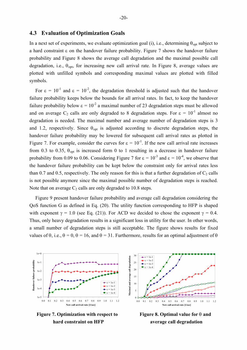
4.3 Evaluation of Optimization Goals

In a next set of experiments, we evaluate optimization goal (i), i.e., determining θopt subject to a hard constraint ε on the handover failure probability. Figure 7 shows the handover failure probability and Figure 8 shows the average call degradation and the maximal possible call degradation, i.e., θopt, for increasing new call arrival rate. In Figure 8, average values are plotted with unfilled symbols and corresponding maximal values are plotted with filled symbols.

For ε = 10-1 and ε = 10-2, the degradation threshold is adjusted such that the handover failure probability keeps below the bounds for all arrival rates. In fact, to keep the handover failure probability below ε = 10-2 a maximal number of 23 degradation steps must be allowed and on average C2 calls are only degraded to 8 degradation steps. For ε = 10-1 almost no degradation is needed. The maximal number and average number of degradation steps is 3 and 1.2, respectively. Since θopt is adjusted according to discrete degradation steps, the handover failure probability may be lowered for subsequent call arrival rates as plotted in Figure 7. For example, consider the curves for ε = 10-1. If the new call arrival rate increases from 0.3 to 0.35, θopt is increased form 0 to 1 resulting in a decrease in handover failure probability from 0.09 to 0.06. Considering Figure 7 for ε = 10-3 and ε = 10-4, we observe that the handover failure probability can be kept below the constraint only for arrival rates less than 0.7 and 0.5, respectively. The only reason for this is that a further degradation of C2 calls is not possible anymore since the maximal possible number of degradation steps is reached. Note that on average C2 calls are only degraded to 10.8 steps.

Figure 9 present handover failure probability and average call degradation considering the QoS function G as defined in Eq. (20). The utility function corresponding to HFP is shaped with exponent γ = 1.0 (see Eq. (21)). For ACD we decided to chose the exponent γ = 0.4. Thus, only heavy degradation results in a significant loss in utility for the user. In other words, a small number of degradation steps is still acceptable. The figure shows results for fixed values of θ, i.e., θ = 0, θ = 16, and θ = 31. Furthermore, results for an optimal adjustment of θ

1e-5

1e-4

1e-3

1e-2

1e-1

1e+0

0.0 0.1 0.2 0.3 0.4 0.5 0.6 0.7 0.8 0.9 1.0 1.1 1.2New call arrival rate [1/sec]

Han

dove

r fa

ilure

pro

babi

lity

e = 1e-1e = 1e-2e = 1e-3e = 1e-4

ε = 1e-1ε = 1e-2ε = 1e-3ε = 1e-4

0

5

10

15

20

25

30

0.0 0.1 0.2 0.3 0.4 0.5 0.6 0.7 0.8 0.9 1.0 1.1 1.2New call arrival rate [1/sec]

Max

imal

and

ave

rage

cal

l deg

rada

tion e = 1e-1

e = 1e-2e = 1e-3e = 1e-4

ε = 1e-1ε = 1e-2ε = 1e-3ε = 1e-4

Figure 7. Optimization with respect to Figure 8. Optimal value for θ and hard constraint on HFP average call degradation

-21-

1e-6

1e-5

1e-4

1e-3

1e-2

1e-1

1e+0

0.0 0.1 0.2 0.3 0.4 0.5 0.6 0.7 0.8 0.9 1.0 1.1 1.2

New call arrival rate [1/sec]

Han

dove

r fa

ilure

pro

babi

lity

q = 0q = 16q = 31q optimal, w = 0.1q optimal, w = 0.5q optimal, w = 0.9

θ = 0θ = 16θ = 31θ optimal, ω = 0.1θ optimal, ω = 0.5θ optimal, ω = 0.9

0

2

4

6

8

10

12

0.0 0.1 0.2 0.3 0.4 0.5 0.6 0.7 0.8 0.9 1.0 1.1 1.2

New call arrival rate [1/sec]

Ave

rage

cal

l deg

rada

tion

q = 16q = 31q optimal, w = 0.1q optimal, w = 0.5q optimal, w = 0.9

θ = 16θ = 31θ optimal, ω = 0.1θ optimal, ω = 0.5θ optimal, ω = 0.9

Figure 9. Optimization with respect to QoS function

0.0

0.2

0.4

0.6

0.8

1.0

0 5 10 15 20 25 30

Degradation threshold θ

Val

ue o

f QoS

func

tion

w = 0.1w = 0.5w = 0.9

ω = 0.1ω = 0.5ω = 0.9

Figure 10. Prioritizing partial goals under the QoS function

with respect to the QoS function for different weights ω are plotted. With weight ω the optimization goal can be prioritized, i.e., ω = 0.1 prioritizes the average call degradation, ω = 0.5 equally weights both QoS measures, whereas ω = 0.9 prioritizes the handover failure probability. Recall, that θ = 0 corresponds to no degradation of C2 calls. Therefore, Figure 9 (right side) does not contain this curve. The figure clearly indicates the effect of the QoS function and the weights on HFP and ACD. Figure 10 plots the QoS function for a fixed call arrival rate of 0.6 calls per second and varying degradation threshold θ. This figure illustrates how the QoS measures HFP and ACD can be prioritized by choosing appropriate weights. The figure exactly plots the functions on which the maximum must be found by subsequent evaluation of the Markov model. For weights ω = 0.1, ω = 0.5, and ω = 0.9 the QoS function is maximal for θ = 1, θ = 9, and θ = 19, respectively.

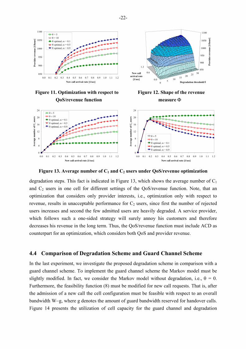
Figure 11 presents results for the QoS/revenue function for different weights ω. With weight ω = 0.1 the average call degradation, i.e., the part representing QoS, is prioritized and with weight ω = 0.9 the revenue measure is prioritized. Results for fixed values of θ, i.e., θ = 5 and θ = 10, are also shown. Figure 12 shows a three-dimensional plot of the revenue measure Φ (see Eq. (22)). In the figure both, call arrival rate and the degradation threshold θ are varied. An increase in revenue can be either observed for increasing new call arrival rate and for increasing C2 call degradation. Under increasing degradation threshold θ, the number of C1 calls also increases since C1 calls are allowed to degrade C2 calls to a number of η·mmax

-22-

850

900

950

1000

1050

1100

0.0 0.1 0.2 0.3 0.4 0.5 0.6 0.7 0.8 0.9 1.0 1.1 1.2

New call arrival rate [1/sec]

Prov

ider

rev

enue

[1/h

our]

q = 5q = 10q optimal, w = 0.1q optimal, w = 0.5q optimal, w = 0.9

θ = 5θ = 10θ optimal, ω = 0.1θ optimal, ω = 0.5θ optimal, ω = 0.9

05

1015 20 25 30

0.0

0.6

1.2850

900

950

1000

1050

1100

Prov

ider

rev

enue

[1/h

our]

Degradation threshold θ

New call arrival rate

[1/sec]

Figure 11. Optimization with respect to Figure 12. Shape of the revenue QoS/revenue function measure Φ

0

4

8

12

16

20

24

0.0 0.1 0.2 0.3 0.4 0.5 0.6 0.7 0.8 0.9 1.0 1.1 1.2

New call arrival rate [1/sec]

Ave

rage

num

ber

of C

1 use

rs

q = 5q = 10q optimal, w = 0.1q optimal, w = 0.5q optimal, w = 0.9

θ = 5θ = 10θ optimal, ω = 0.1θ optimal, ω = 0.5θ optimal, ω = 0.9

0

4

8

12

16

20

24

0.0 0.1 0.2 0.3 0.4 0.5 0.6 0.7 0.8 0.9 1.0 1.1 1.2

New call arrival rate [1/sec]

Ave

rage

num

ber

of C

2 use

rs

q = 5q = 10q optimal, w = 0.1q optimal, w = 0.5q optimal, w = 0.9

θ = 5θ = 10θ optimal, ω = 0.1θ optimal, ω = 0.5θ optimal, ω = 0.9

Figure 13. Average number of C1 and C2 users under QoS/revenue optimization

degradation steps. This fact is indicated in Figure 13, which shows the average number of C1 and C2 users in one cell for different settings of the QoS/revenue function. Note, that an optimization that considers only provider interests, i.e., optimization only with respect to revenue, results in unacceptable performance for C2 users, since first the number of rejected users increases and second the few admitted users are heavily degraded. A service provider, which follows such a one-sided strategy will surely annoy his customers and therefore decreases his revenue in the long term. Thus, the QoS/revenue function must include ACD as counterpart for an optimization, which considers both QoS and provider revenue.

4.4 Comparison of Degradation Scheme and Guard Channel Scheme

In the last experiment, we investigate the proposed degradation scheme in comparison with a guard channel scheme. To implement the guard channel scheme the Markov model must be slightly modified. In fact, we consider the Markov model without degradation, i.e., θ = 0. Furthermore, the feasibility function (8) must be modified for new call requests. That is, after the admission of a new call the cell configuration must be feasible with respect to an overall bandwidth W−g, where g denotes the amount of guard bandwidth reserved for handover calls. Figure 14 presents the utilization of cell capacity for the guard channel and degradation

-23-

40

50

60

70

80

90

100

0.00 0.05 0.10 0.15 0.20 0.25 0.30 0.35 0.40 0.45 0.50

New call arrival rate [1/sec]

Ave

rage

cel

l cap

acity

util

izat

ion

[%]

Degradation schemeGuard channel, e = 1e-1Guard channel, e = 1e-2Guard channel, e = 1e-3Guard channel, e = 1e-4

Degradation schemeGuard channel, ε = 1e-1Guard channel, ε = 1e-2Guard channel, ε = 1e-3Guard channel, ε = 1e-4

1e-3

1e-2

1e-1

1e+0

0.00 0.05 0.10 0.15 0.20 0.25 0.30 0.35 0.40 0.45 0.50

New call arrival rate [1/sec]

CB

P du

e to

gua

rd c

hann

el r

eser

vatio

n

e = 1e-1e = 1e-2e = 1e-3 e = 1e-4

ε = 1e-1ε = 1e-2ε = 1e-3ε = 1e-4

Figure 14. Utilization of cell capacity: Figure 15. New call blocking guard channel vs. degradation scheme probability for guard channel scheme

scheme for increasing new call arrival rate. For every new call arrival rate, the degradation threshold θ as well as the amount of guard bandwidth g is optimized according to a hard constraint ε on the handover failure probability. For a fair comparison of both schemes we consider η = 0 in the degradation scheme, i.e., new C1 calls cannot degrade ongoing C2 calls. Furthermore, in the guard channel scheme the (constant) bitrate requirement of C2 calls is determined according to the average bitrate that C2 calls receive in the degradation scheme in a corresponding experiment. Note that these restrictions are only applied to make the arrival process and required bitrate of new calls in both schemes comparable and thus a fair comparison between both schemes can be performed. The results of this comparison are not affected even without these restrictions.

Note that Figure 14 shows only one curve for the degradation scheme since the utilization of cell capacity is the same for each value of ε. Comparing the curves for the guard channel scheme we conclude that a huge amount of bandwidth is wasted in order to achieve the constraint on handover failure probability. In other words, the more stringent the constraint the more bandwidth must be reserved for handover calls and the higher the probability that this bandwidth is unused. This effect can be observed from Figure 15, which shows the probability of rejecting a new call request although sufficient cell capacity to accommodate the call is available. In fact, if the cell gets saturated most new calls are rejected since capacity is reserved for handover calls but currently unused. As a conclusion we argue that for future mobile networks that support service degradation, the degradation scheme is the method of choice since it can guarantee a certain handover failure probability and also high capacity utilization.

5 QoS/Revenue Management Framework in Practice

5.1 Implementation Issues

In this section, we discuss implementation issues for the proposed QoS/revenue management framework. As outlined in Section 2, the QoS/revenue management framework comprises two

-24-

new components introduced in this paper: (1) the admission controller and (2) the QoS/revenue management unit for optimization of the threshold for maximal bandwidth degradation. The computations performed by the admission controller to decide whether admitting or rejecting a call introduces no additional overhead compared to traditional admission control schemes since only simple decisions have to be made. When the admission controller decides to degrade/upgrade current C2 calls to a specified bandwidth, additional signaling is required in order to notify the corresponding mobile terminals.

The overhead that is induced by the QoS/revenue management unit is twofold. First, in order to find the optimal setting for the degradation threshold θ, the Markov model has to be evaluated several times at the end of each control period. As stated in the Section 4, this evaluation requires just a few seconds of CPU time due to the small state space of the Markov model. Moreover, results of previously computed parameterizations of the Markov model can easily be cached avoiding the repetition of identical evaluations of the Markov model in subsequent control periods. Second, the Markov model requires monitored traffic characteristics gathered by the online traffic measurement unit. Precisely, arrivals of C1 and C2 new call requests and handovers as well as the cell residence times are monitored online in each control period. An exponential-weighted moving average technique from time series analysis is adopted to compute the expected arrival rates λn,1, λn,2, λh,1, λh,2, and the expected residence time 1/µ at the end of each control period from the values monitored during the current control period and the estimated values from the last control period. Let (m)

nϕ be the average rate corresponding to the monitored values during control period n and let (e)

n 1−ϕ be the estimated arrival rate at the end of control period n-1. Then, the new estimate for control period n is computed by

(e)(e) (m)n nn 1 (1 )−ϕ = ρ⋅ϕ + − ρ ⋅ϕ . (23)

The coefficient ρ ∈ [0,1] has to be properly selected to smooth the estimated values. In general, a small value ρ can keep track of the changes more accurately, but is perhaps too heavily influenced by temporary fluctuations. On the other hand, a large value of ρ results in a more stable estimation, i.e., more history is considered, but could be too slow in adapting to real traffic changes. Recently, more sophisticated techniques are proposed for estimating future traffic load in mobile networks based on heuristics to improve the exponential-weighted moving average technique [14].

Besides the estimation of arrival rates and residence time, monitored values for the average number of users in neighboring cells as well as the average number of degradation steps in neighboring cells are communicated to the target cell. Note that in general the target cell and the neighboring cells are controlled by the same base station controller and thus no expensive signaling messages are required. Figure 16 summarizes the actions performed at the end of each control period in order to determine the optimal value of the degradation threshold θ.

-25-

(1) Determine current traffic pattern by online traffic monitoring according to Eq. (23) (2) Initialize θ = 0 and gmax = 0 (3) Solve the global balance equations πθ·Qθ = 0 together with the normalization condition

|πθ| = 1, for the given traffic pattern and degradation threshold θ. (4) Determine the QoS and revenue measures from the steady state solution of the Markov

model according to Eqs. (11) to (16) and Eq. (22). (5) Evaluate the QoS/revenue function (20) with utility function (21) depending on the

predefined optimization goal. Let g be the outcome of the QoS/revenue function (20). (6) IF g > gmax THEN DO (7) gmax = g (8) θopt = θ (9) OD (10) θ = θ + δ (11) IF θ < R THEN restart calculation with step (3)

Figure 16. Algorithm for determining θopt at the end of each control period

Finally we discuss how management of user profiles as well as call charging can be accomplished. Each user profile has to comprise the user's QoS class, i.e., high or low priority class which is stored in the customer database of the provider, e.g., the home location register in UMTS [12]. For charging C2 calls the current bitrate granted by the admission controller, i.e., R−m·δ kbps, has to be taken into account during call duration. This is unnecessary for C1 calls which have a constant bitrate R. In UMTS networks, this call charging can be processed by the subscription management component of the operation subsystem using a user's profile. Utilizing these existing charging mechanisms, no additional signaling overhead arises for charging real-time services.

5.2 Simulation Results for the QoS/Revenue Management Framework

Using simulation experiments, we illustrate the benefit of the proposed integrated framework for adaptive online optimization of the admission controller. The simulator considers a cluster of seven cells with the target cell in the center as presented in Figure 5. Furthermore, the simulator contains the implementation of the algorithmic procedure presented in Figure 16 in order to determine the optimal value θopt for the degradation threshold in control periods of fixed duration ∆t. Subsequently, the degradation threshold of the simulator is updated according to the optimal value θopt determined from the Markov model. In [15], measurements have been taken over several weeks in order to derive a typical daily usage pattern, i.e., a traffic model for mean arrival rates of new calls with respect to the time of day. Table 2 presents the first part (half day window) of this daily usage pattern, i.e., the mean arrival rates of new calls for 0 a.m. up to 12 a.m. These arrival rates are utilized in the following experiments in order to evaluate the effectiveness of the proposed adaptive call admission control scheme within a transient scenario.

-26-

1 2 3 4 5 6 7 8 9 10 11 12New call

arrival rate 0.49 0.57 0.60 0.48 0.62 0.55 0.68 0.87 0.96 1.20 1.15 1.06

Hour

Table 2. Half day window of a daily usage pattern

Figure 17 depicts the average call degradation in every control period for the transient scenario. In both figures the average call degradation with knowledge of the current new call arrival rate and the average call degradation with respect to the online monitored traffic pattern is shown. The figures differ in the length of the control periods, i.e., in Figure 17 (left side) a control period has duration ∆t = 2 minutes and in Figure 17 (right side) a control period is of duration ∆t = 5 minutes, respectively. The value ρ corresponding to the exponential-weighted moving average is assumed to be 0.7 in order to consider more history in the traffic estimation process. In both experiments the optimization is performed according to optimization goal (ii). The QoS function G as defined in Eq. (20) is considered with ω = 0.9, i.e., handover calls are prioritized.

The purpose of these experiments is to study how fast the online QoS/revenue management can adapt the degradation threshold to changing traffic conditions over several control periods. Comparing both figures, we find larger fluctuations in the average call degradation but also faster adaptation to the optimal value in Figure 17 (left side), as expected. Due to the shorter control periods, less call arrivals are counted during a control period leading to higher fluctuations in the monitored arrival rate. Considering Figure 17 (right side), we find a more stable but also slower adaptation of the threshold. For example consider the end of the second hour of the experiments in Figure 17. The left side of Figure 17 shows a quite fast reduction in average call degradation from about 4 to 3 calls due to a fast adaptation of the degradation threshold whereas the adaptation requires much more time with longer control periods (see right side of Figure 17).

2

3

4

5

6

7

8

9

0 1 2 3 4 5 6 7 8 9 10 11 12Time [hour]

Ave

rage

cal

l deg

rada

tion

controlledoptimal

2

3

4

5

6

7

8

9

0 1 2 3 4 5 6 7 8 9 10 11 12Time [hour]

Ave

rage

Cal

l Deg

rada

tion

controlledoptimal

Figure 17. Adjustment of degradation threshold for control periods of ∆t = 2 minutes (left side) and ∆t = 5 minutes (right side)

-27-

Conclusions

We presented a novel call admission control and bandwidth degradation scheme for real-time traffic. For online optimization of the admission controller we developed an efficiently analyzable Markov model that incorporates important features of 3G cellular networks, such as CDMA intra- and inter-cell interference, different call priorities and soft handover. Using parameter estimation techniques, the Markov model is periodically customized with parameters corresponding to currently measured traffic in the radio access network. Thus, the presented approach allows the effective online management of both quality of service (QoS) for mobile users and provider revenue in CDMA cellular networks. In fact, the proposed QoS/revenue management not only closes the loop between network operation and network control, but also quickly reacts to changing traffic load.

We presented curves for measures of interest derived from the numerical steady state analysis of the Markov model. In particular, we compare the effectiveness of the proposed adaptive bandwidth degradation scheme with existing approaches based on adaptive guard channels. We conclude that for 3G networks with different QoS classes and call priorities, the graceful degradation of bandwidth should be the method of choice for prioritization of handover calls. This is because in the guard channel scheme is a high probability that a new call request will be rejected, although bandwidth is still available, i.e., the guard channels are unused.

References

[1] 3GPP, QoS Concept and Architecture, Technical Specification TS 23.107, Mar. 2002. http://www.3gpp.org.

[2] M. Ajmone Marsan, S. Marano, C. Mastroianni, and M. Meo, Performance Analysis of Cellular Mobile Communication Networks Supporting Multimedia Services, Mobile Networks and Applications (MONET) 5, 167-177, 2000.

[3] A.T. Campbell, R.R.-F. Liao, A Utility-Based Approach for Quantitative Adaptation in Wireless Packet Networks, Wireless Networks 7, 541-557, 2001.

[4] I. Chlamtac, S.K. Das, and G. Záruba, A Prioritized Real-Time Wireless Call Degradation Framework for Optimal Call Mix Selection, Mobile Networks and Applications 7, 143-151, 2002.

[5] S. Choi and K.G. Shin, A Comparative Study of Bandwidth Reservation and Admission Control Schemes in QoS-Sensitive Cellular Networks, Wireless Networks 6, 289-305, 2000.

-28-

[6] C.T. Chou and K.G. Shin, Analysis of Combined Adaptive Bandwidth Allocation and Admission Control in Wireless Networks, Proc. 21th Conf. on Computer Communications (IEEE Infocom), New York, 2002.

[7] S.K. Das, R. Jayaram, N.K. Kakani, and S.K. Sen, A Call Admission and Control Scheme for Quality-of-Service Provisioning in Next Generation Wireless Networks, Wireless Networks 6, 17-30, 2000.

[8] J.S. Evans and D. Everitt, Effective Bandwidth-Based Admission Control for Multiservice CDMA Cellular Networks, IEEE Trans. on Vehicular Technology 48, 36-46, 1999.

[9] J.S. Evans and D. Everitt, On the Teletraffic Capacity of CDMA Cellular Networks, IEEE Trans. on Vehicular Technology 48, 153-165, 1999.

[10] ETSI, Universal Mobile Telecommunication System (UMTS); Selection Procedures for the Choice of Radio Transmission Technologies of the UMTS, Technical Report TR 101 112 v3.2.0, 1998.

[11] K.S. Gilhousen, I.M. Jacobs, R. Padovani, A.J. Viterbi, L.A. Weaver, and C.E. Wheatley, On the Capacity of a Cellular CDMA System, IEEE Trans. on Vehicular Technology 40, 303-312, 1991.

[12] H. Kaaranen, A. Ahtiainen, L. Laitinen, S. Naghian, and V. Niemi, UMTS Networks, Architecture, Mobility and Services, John Wiley & Sons, 2001.

[13] G. Karmani and K.N. Sivarajan, Capacity Evaluation for CDMA Cellular Systems, Proc. 20th Conf. on Computer Communications (IEEE Infocom), Anchorage, Alaska, 601-610, 2001.

[14] M. Kim and B. Noble, Mobile Network Estimation, Proc. 7th Int. Conf. on Mobile Computing and Networking (MobiCom), Rome, Italy, 298-309, 2001.

[15] A. Klemm, C. Lindemann, and M. Lohmann, Traffic Modeling and Characterization for UMTS Networks, Proc. IEEE Globecom, San Antonio, Texas, 1741-1746, 2001.

[16] O. Lataoui, T. Rachidi, L. G. Samuel, S. Gruhl, and R. Yan, A QoS Management Architecture for Packet Switched 3rd Generation Mobile Systems, NetWorld+Inerop2000 - Engineers Conference on Broadband Internet Access Technologies Systems & Services, 2000.

[17] W.C.Y. Lee, Overview of Cellular CDMA, IEEE Trans. on Vehicular Technology 40, 291-302, 1991.

[18] K.D. Lee and S. Kim, Optimization for Adaptive Bandwidth Reservation in Wireless Multimedia Networks, Computer Networks 38, 631-643, 2002.

[19] V.C.M. Leung and F. Yu, Mobility-Based Predictive Call Admission Control and Bandwidth Reservation in Wireless Cellular Networks, Proc. 20th Conf. on Computer Communications (IEEE Infocom), Anchorage, Alaska, 518-526, 2001.

-29-

[20] C. Lindemann, M. Lohmann, and A. Thümmler, Adaptive Performance Management for UMTS Networks, Computer Networks, 38, 477-496, 2002.

[21] C. Lindemann, M. Lohmann, and A. Thümmler, A Unified Approach for Improving QoS and Provider Revenue in 3G Mobile Networks, Mobile Networks and Applications 8, 209-221, 2003.

[22] Y. Ma, J.J. Han, and K.S. Trivedi, Call Admission Control for Reducing Dropped Calls in Code Division Multiple Access (CDMA) Cellular Systems, Computer Communications 25, 689-699, 2002.

[23] V. Mainkar and K.S. Trivedi, Sufficient Conditions for Existence of a Fixed Point in Stochastic Reward Net-Based Iterative Models, IEEE Trans. on Software Engineering 22, 640-653, 1996.

[24] B. Melis and G. Romano, UMTS W-CDMS: Evaluation of Radio Performance By Means of Link Level Simulations, IEEE Personal Communications 7, 42-49, 2000.

[25] R. Ramjee, R. Nagarajan, and D. Towsley, On Optimal Call Admission Control in Cellular Networks, Proc. 15th Conf. on Computer Communications (IEEE Infocom), San Francisco, CA, 43-50, 1996.

[26] A.J. Viterbi, A.M. Viterbi, and E. Zehavi, Other-Cell Interference in Cellular Power-Controlled CDMA, IEEE Trans. on Communications 42, 1501-1504, 1994.

[27] Y. Zhang and D. Liu, An Adaptive Algorithm for Call Admission Control in Wireless Networks, Proc. IEEE Globecom, San Antonio, Texas, 3628-3632, 2001.

[28] M. Zorzi, On the Analytical Computation of the Interference Statistics with Applications to the Performance Evaluation of Mobile Radio Systems, IEEE Trans. on Communications 45, 103-109, 1997.