Adaptive Control of a Hybrid Powertrain with

Map-based ECMS

Martin Sivertsson, Christofer Sundström and Lars Eriksson

Linköping University Post Print

N.B.: When citing this work, cite the original article.

Original Publication:

Martin Sivertsson, Christofer Sundström and Lars Eriksson, Adaptive Control of a Hybrid

Powertrain with Map-based ECMS, 2011, IFAC World Congress 2011.

Copyright: International Federation of Automatic Control

Postprint available at: Linköping University Electronic Press

http://urn.kb.se/resolve?urn=urn:nbn:se:liu:diva-84957

Adaptive Control of a Hybrid Powertrainwith Map-based ECMS

Martin Sivertsson ∗, Christofer Sundstrom ∗, andLars Eriksson ∗

∗ Vehicular Systems, Dept. of Electrical Engineering, LinkopingUniversity, SE-581 83 Linkoping, Sweden, {marsi,csu,larer}@isy.liu.se.

Abstract: To fully utilize the fuel reduction potential of a hybrid powertrain requires a carefuldesign of the energy management control algorithms. Here a controller is created using map-based equivalent consumption minimization strategy and implemented to function without anyknowledge of the future driving mission. The optimal torque distribution is calculated offline andstored in tables. Despite only considering stationary operating conditions and average batteryparameters, the result is close to that of deterministic dynamic programming. Effects of makingthe discretization of the tables sparser are also studied and found to have only minor effects onthe fuel consumption. The controller optimizes the torque distribution for the current gear aswell as assists the driver by recommending the gear that would give the lowest consumption.Two ways of adapting the control according to the battery state of charge are proposed andinvestigated. One of the adaptive strategies is experimentally evaluated and found to ensurecharge sustenance despite poor initial values.

Keywords: Hybrid Vehicles, Adaptive Control, Automotive Control, Optimal Control

1. INTRODUCTION

A hybrid powertrain utilizes at least two separate energyconverters. This has the potential to significantly increasethe efficiency of the powertrain. The key to utilizingthe full potential of the powertrain lies in the designof the control algorithm. The goal in hybrid powertraincontrol is normally to minimize the fuel consumption whilemaintaining the battery State of Charge (SOC) withinprescribed limits, sometimes with addition of constraintsregarding emissions.

This paper develops an adaptive Equivalent ConsumptionMinimization Strategy (ECMS), based on Musardo andRizzoni (2005), and applies it to the Haldex electric TorqueVectoring Drive (eTVD). The optimal torque distributionis calculated offline and stored in tables and the effectsof discretization on the fuel consumption is studied. Thentwo ways of adapting the control to maintain the SOCwithin the desired limits are investigated.

1.1 The Haldex eTVD and the test vehicle

The system used for modeling, simulation, and experimen-tal evaluation is a SAAB 9-3 XWD with a 2.0L turbocharged spark ignited combustion engine and a six-speedmanual gear-box (GB), fitted with the eTVD.

The eTVD is a system designed to combine all-wheeldrive (AWD) with hybrid functionality. It also has theability to control the torque distribution on the rearwheels individually, which is useful to prevent under-and over-steering. In the eTVD concept the combustionengine (ICE) and main electric motor (EM) are connectedelectrically to each other via the generator (ISG) and

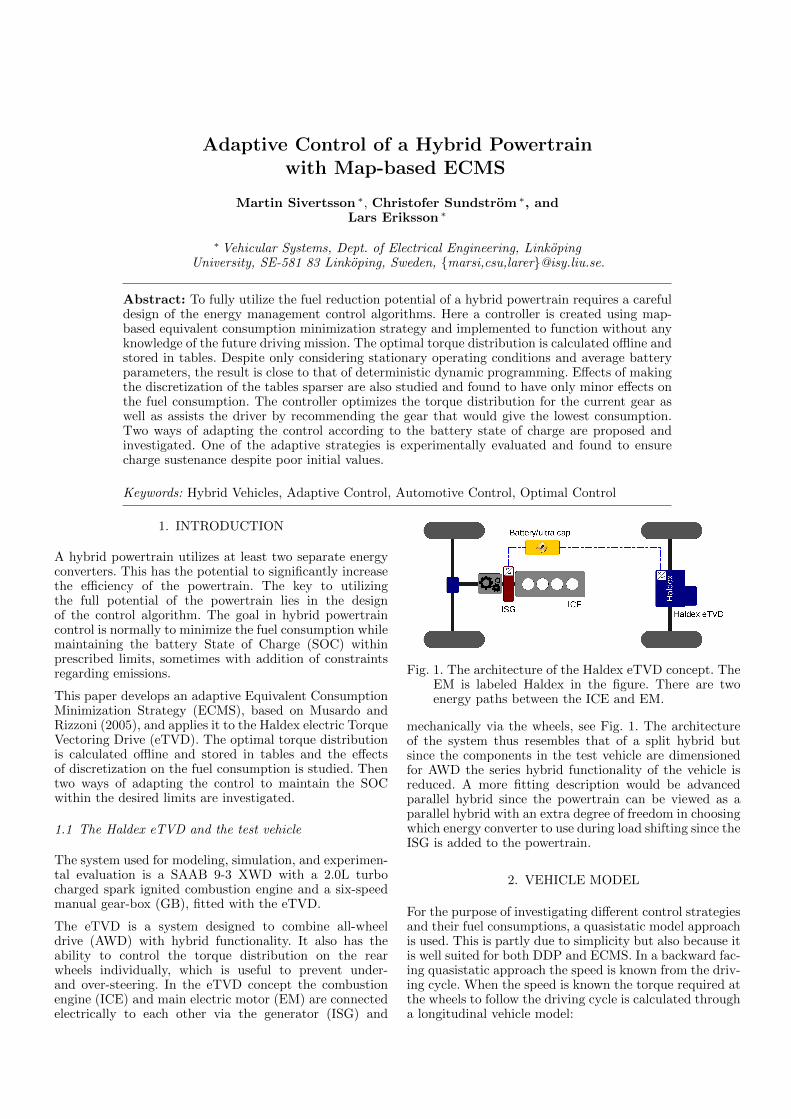
Fig. 1. The architecture of the Haldex eTVD concept. TheEM is labeled Haldex in the figure. There are twoenergy paths between the ICE and EM.

mechanically via the wheels, see Fig. 1. The architectureof the system thus resembles that of a split hybrid butsince the components in the test vehicle are dimensionedfor AWD the series hybrid functionality of the vehicle isreduced. A more fitting description would be advancedparallel hybrid since the powertrain can be viewed as aparallel hybrid with an extra degree of freedom in choosingwhich energy converter to use during load shifting since theISG is added to the powertrain.

2. VEHICLE MODEL

For the purpose of investigating different control strategiesand their fuel consumptions, a quasistatic model approachis used. This is partly due to simplicity but also because itis well suited for both DDP and ECMS. In a backward fac-ing quasistatic approach the speed is known from the driv-ing cycle. When the speed is known the torque required atthe wheels to follow the driving cycle is calculated througha longitudinal vehicle model:

Treq=rw

( ρa2CDAfV (t)2︸ ︷︷ ︸

Fair

+mgfr︸ ︷︷ ︸Froll

+mV (t)︸ ︷︷ ︸Facc

+ V (t)Jwr2w︸ ︷︷ ︸

Fwi

)(1)

where Fair is the aerodynamic drag, Froll the rollingresistance, Fwi the inertia of the wheels, and Facc is theacceleration force. Force from road grade is neglected.

2.1 Components

The control signals of the system are the energy convertertorques TICE , TISG, TEM , and gear γGB . The components(ICE, EM, ISG and GB) are all modeled with a powerbalance and efficiency, Pout = Pinη, where the efficiencies,η, are assumed to be known and account for all losses in thecomponent. The efficiency ηGB is assumed constant whilethe efficiencies of the energy converters are shown in Fig. 2.The battery is modeled as a Thevenin equivalent circuitwith open circuit voltage Uoc(SOC), coloumbic chargeefficiency ηc(SOC), and constant internal resistance Ri.The battery in the test vehicle outputs its SOC, thusthe SOC is assumed to be known. The power required bythe auxiliary units, Paux, is assumed constant. For moredetails about the modeling see Sivertsson (2010).

3. REFERENCE CONSUMPTIONS

As a reference for the implemented optimization, deter-ministic dynamic programming (DDP) as described inGuzzella and Sciarretta (2007) is used. Time and SOC arediscretized with a step length of 1s and 0.02h respectively.The SOC discretization is chosen so that one step roughlyequals the change in SOC from the auxiliary units during1s. The operating points from the DDP solution to NEDCare shown in Fig. 2. Interesting to note is the efficientuse of the ISG in load shift and that almost all the EMsoperating points during braking are on, or close, to thetorque limit. This is a result of the EM and ISG primarilybeing designed for torque vectoring and AWD and not fueleconomy.

To evaluate the performance of the real-time control, theconsumption as a strictly AWD vehicle is used. For thatpurpose a control is used where the gear that results inthe lowest consumption at each time is engaged. The EMis assumed to be unused both in traction and braking, thusthis mode corresponds to pure ICE propulsion.

4. THE ECMS

In ECMS, proposed in Paganelli et al. (2001) and Paganelliet al. (2002), the sum of fuel and fuel equivalent of theelectrical power is minimized. Since fuel and battery powerare not directly comparable an equivalence factor, λ, isused. The function to be minimized can be written as:

H = Pf (TICE , γGB) + λ(t)Pbatt(TEM , TISG, γGB) (2)

Under the assumption that the battery efficiency is in-dependent of SOC, the equivalence factor λ remains ap-proximately constant along the optimal trajectory. There-fore the optimization problem is reduced to finding theconstant λ that approximates the optimal trajectory of agiven driving cycle. Since the characteristics of the batterydepends on if the battery is charging or discharging, λ

2000 4000 60000

50

100

150

200

250

0.040.080.12

0.16

0.160.16

0.2

0.2

0.2

0.2

0.2

0.22

0.22

0.220.22

0.24

0.24

0.24

0.24

0.24

0.24

0.24

0.26

0.26

0.26

0.26

0.26

0.26

0.26

0.28

0.28

0.28

0.28

0.28

0.28

0.28

0.29

50.

295

0.295

0.29

5

0.29

5

0.295

0.295

0.31

0.31

0.31

0.310.31

0.31

0.325

0.325

0.325

0.325

ICE

WICE

[rpm]

TIC

E [N

m]

0 2000400060008000−40

−20

0

20

40

60

80

100

0.65

0.7

0.7

0.7

0.75

0.75

0.75

0.75

0.8

0.8

0.8

0.8

0.8

0.82

5

0.82

5

0.825

0.8250.825

0.82

5

0.825

0.85

0.85

0.85

0.87

5

0.87

5

0.9

WEM

[rpm]

TE

M [N

m]

EM

TractionRegeneration

0.5 1 1.5

x 104

0

1

2

3

4

5

6

7

8

0.650.7

0.7

0.7

0.7

0.75

0.75

0.75

0.75

0.8

0.8

0.80.80.815

0.815

0.81

5

0.815

0.830.83

0.83

0.83

0.84

5

0.8450.845

0.84

5

0.8450.845

0.86

0.860.86 0.

86

0.860.86

0.87

5

0.875

0.875

0.875

0.875

0.89

0.89

0.890.9050.905

WISG

[rpm]

TIS

G [N

m]

ISG

Load ShiftRegeneration

Fig. 2. Efficiencies of the ICE, EM, and ISG, as well as theoperating points of the three energy converters on theNEDC from the DDP solution

is sometimes replaced by two constants. It is howevershown in Musardo and Rizzoni (2005) that one constantsuffices to get a good approximation on a given drivingcycle, which is the approach selected here. For more detailson ECMS see Guzzella and Sciarretta (2007); Pisu andRizzoni (2007); Sciarretta et al. (2004).

As a consequence of the discussion above the strategy forselecting the control inputs becomes:

[TICE , TISG, TEM , γGB ] = argmin(H) (3)

Subject to:

Treq = ηGBγGB (TICE − γISGTISG) + γEMTEM (4a)

TEM,min(ωEM ) ≤TEM ≤ TEM,max(ωEM ) (4b)

0 ≤TICE≤ TICE,max(ωICE) (4c)

0 ≤TISG ≤ TISG,max(ωISG) (4d)

Pbatt,min(SOC) ≤Pbatt ≤ Pbatt,max(SOC) (4e)

4.1 Offline Optimization

Instead of solving the computationally demanding threedegree of freedom problem in (3)-(4) for all possible con-trols in real-time, the optimization is performed offline andthe result is tabulated. In the real-time implementation thecontrol system interpolates in the stored data to find theoptimal torque distribution.

In the offline calculations the three parameters that theECMS algorithm takes as input, i.e. vehicle speed, requiredtorque, and equivalence factor, are discretized and theoptimal torque distribution on the three energy converters,as well as the optimal gear, are calculated as a functionof (V ,Treq,λ) for each point. Since, for each gear, it is atwo degree of freedom problem, see (4a), it requires twotables for each gear, one for the ISG and one for the ICE.From these two tables the torque required from the EMcan be calculated using (4a). With six gears, not includingreverse, a total of 13 tables are calculated: six ICE, sixISG and one for the gear selection. So the system notonly optimizes the torque distribution for the current gear,it also assists the driver by recommending the gear thatwould give the lowest fuel consumption.

0 0.5 1 1.5 2 2.5 3 3.5 4 4.5 5

0

200

400

600

λ

Tor

ques

[Nm

]

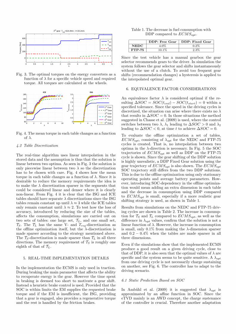
3rd gear Treq

=524.4Nm ; V=20.2m/s

TICE

TISG

TEM

Fig. 3. The optimal torques on the energy converters as afunction of λ for a specific vehicle speed and requiredtorque. All torques are calculated at the wheels.

0 2 4 6 8 1060

80

100

120

140

160

180

λ

TIC

E,m

ean

ICE

0 2 4 6 8 100

0.5

1

1.5

2

2.5

3

3.5

λ

TIS

G,m

ean

ISG

1st Gear

2nd Gear

3rd Gear

4th Gear

5th Gear

6th Gear

Fig. 4. The mean torque in each table changes as a functionof λ.

4.2 Table Discretization

The real-time algorithm uses linear interpolation in thestored data and the assumption is thus that the solution islinear between two optima. As seen in Fig. 3 the solution isonly piecewise linear between two λ so the discretizationhas to be chosen with care. Fig. 4 shows how the meantorque in each table changes as a function of λ. Since it isdesirable to reduce the memory requirements the idea isto make the λ discretization sparser in the segments thatcould be considered linear and denser where it is clearlynon-linear. From Fig. 4 it is clear that the ISG and ICEtables should have separate λ discretizations since the ISGtables remain constant up until λ ≈ 3 while the ICE tablesonly remain constant until λ ≈ 2. To test how the loss ofaccuracy, introduced by reducing the size of the tables,affects the consumption, simulations are carried out ontwo sets of tables: one large set, TL, and one small set,TS . The TL has the same V- and Treq-discretization asthe offline optimization itself, but the λ-discretization ismade sparser according to the strategy mentioned above.The TS-discretization is made sparser than TL in all threedirections. The memory requirement of TS is roughly oneeighth of that of TL.

5. REAL-TIME IMPLEMENTATION DETAILS

In the implementation the ECMS is only used in traction.During braking the main parameter that affects the abilityto recuperate energy is the gear. However the time spentin braking is deemed too short to motivate a gear shift.Instead a heuristic brake control is used. Provided that theSOC is within limits the EM supplies the requested braketorque and if the EM is insufficient, the ISG, providingthat a gear is engaged, also provides a regenerative torqueand the rest is handled by the friction brakes.

Table 1. The decrease in fuel consumption withDDP compared to ECMSopt.

DDP: Free Gear DDP: Fixed Gear

NEDC 4.0% 0.2%

FTP-75 10.1% 2.3%

Since the test vehicle has a manual gearbox the gearselector recommends gears to the driver. In simulation thesystem follows the gear selector and shifts instantaneouslywithout the use of a clutch. To avoid too frequent gearshifts (recommendation changes) a hysteresis is applied tothe interpolated optimal gear.

6. EQUIVALENCE FACTOR CONSIDERATIONS

An equivalence factor λ is considered optimal if the re-sulting ∆SOC = SOC(tend) − SOC(tstart) = 0 within aspecified tolerance. Since the speed in the driving cycles isdiscretized, the situation can arise where there exists no λthat results in ∆SOC = 0. In those situations the methodsuggested in Chasse et al. (2009) is used, where the controlswitches between two λ, λ1 leading to ∆SOC > 0 and λ2leading to ∆SOC < 0, at time t to achieve ∆SOC = 0.

To evaluate the offline optimization a set of tables,ECMSopt, consisting of λopt for the NEDC and FTP-75cycles is created. That is, no interpolation between twooptima in the λ-direction is necessary. In Fig. 5 the SOCtrajectories of ECMSopt as well as DDP on the FTP-75cycle is shown. Since the gear shifting of the DDP solutionis highly unrealistic, a DDP Fixed Gear solution using thegear trajectory of ECMSopt is also shown. The ECMSopt

SOC trajectory still differs from the two DDP solutions.This is due to the offline optimization using only stationaryoperating points and average battery parameters. How-ever, introducing SOC-dependency in the offline optimiza-tion would mean adding an extra dimension in each tableand the decrease in consumption using DDP comparedto ECMSopt is small, especially if a more realistic gearshifting strategy is used, as shown in Table 1.

Results from simulations on the NEDC and FTP-75 driv-ing cycles are shown in Table 2. The increase in consump-tion for TS and TL compared to ECMSopt, as well as thedifference in λopt values, confirm that the solution is not alinear function of λ. However, the increase in consumptionis small, only 0.1% from making the λ-dimension sparserand 0.2 − 0.4% when the tables are made sparser in allthree dimensions.

Even if the simulations show that the implemented ECMSproduce a good result on a given driving cycle, close tothat of DDP, it is also seen that the optimal values of λ arespecific and the system seems to be quite sensitive. A λoptfrom one driving cycle is not necessarily charge sustainingon another, see Fig. 6. The controller has to adapt to thedriving scenario.

6.1 Static Prediction Based on SOC

In Ambuhl et al. (2009) it is suggested that λopt isapproximated by an affine function in SOC. Since theeTVD mainly is an AWD concept, the charge sustenanceof the controller is crucial. Therefore another adaptation

0 200 400 600 800 1000 1200 1400 1600 1800

40

42

44

46

48

50

52

54

t [s]

SO

C [%

]

Comparison ECMS vs. DDP, FTP−75

ECMSopt

DDP Fixed GearDDP Free Gear

Fig. 5. The optimal SOC trajectory on the FTP-75 cyclewith ECMS and DDP. The offline optimization resultsin a different SOC trajectory than DDP, mainly dueto the nominal battery parameters used.

Table 2. λopt and associated consumptionof the different tables. Consumptions are inL/100km and Reduction is compared to AWD.

Cycle Performance EMCSopt TL TS

NEDCλopt 2.8384 2.8238 2.8426

Consumption 5.728 5.733 5.738Reduction 17.23 % 17.15 % 17.08 %

FTP-75λopt 2.6353 2.6615 2.7146

Consumption 5.505 5.512 5.534Reduction 24.33 % 24.23 % 23.93 %

0 1000 2000 3000 4000 50000

5

10

15

20

25

30

35Velocity Profile, NEDC repeated five times

V [m

/s]

0 1000 2000 3000 4000 500010

20

30

40

50

60

70

t [s]

SO

C [%

]

λopt,FTP−75

λopt,NEDC

λopt,FTP−75

+SP

Fig. 6. The NEDC cycle repeated five times withλopt,NEDC , λopt,FTP−75 and λopt,FTP−75 with the useof Static Prediction based on SOC. The system issensitive to the equivalence factors. The λopt for onedriving cycle leads to poor performance on another,but with the adaptive control the system is chargesustaining.

function is suggested. Under the assumption that thereexists one λ that approximates a given driving cycle,the controller should ideally find that λ for the futuredriving mission and use that value for the entire mission.To allow the system to use as much of the batterycapacity as possible the idea is to create a functionthat is relatively flat around the center of the desiredSOC window. However, when the SOC approaches thelimits of the SOC window it needs to adapt to ensurecharge sustenance. The chosen function that fulfills theserequirements is a tangens function, see Fig. 7-left. The

30 40 50 60 70SOC [%]

kc

λc

0 200 400 600 800 1000

30

35

40

45

50

55

60

65

70

t [s]

SO

C [%

]

SOC trajectories as a result of optimal and non−optimal λc for different slopes

kc= −1.0 λ

c,opt=2.7766 Fuel Consumption= 5.734 L/100km

kc= −1.9 λ

c,opt=2.7300 Fuel Consumption= 5.735 L/100km

kc= −4.1 λ

c,opt=2.5894 Fuel Consumption= 5.743 L/100km

kc= −7.0 λ

c,opt=2.4158 Fuel Consumption= 5.753 L/100km

Fig. 7. Left: The shape of the function used for adaptivecontrol. Right: SOC trajectories for different slopeson the NEDC cycle with λc,opt as well as with λc = 4.The plot indicates that a steeper slope is more ableto keep the SOC within the limits but it also showsthat a steep slope alone does not guarantee that theSOC stays within the desired SOC window. A steepslope also increases the consumption.

Table 3. λc,opt and associated consumptions.Consumptions are in L/100km and reduction

is compared to AWD.

Cycle Performance TL TS

NEDCλc,opt 2.73 2.7374

Consumption 5.735 5.739Reduction 17.12 % 17.07 %

FTP-75λc,opt 2.6365 2.6823

Consumption 5.515 5.533Reduction 24.19 % 23.95 %

adaptation of λ is of the form:

λ = fSP (λc, kc, SOC) (5)

where fSP has the shape of a tangens function centeredat λc, with the slope kc. As seen in Fig. 7-right thefuel consumption increases with the slope but it is alsoapparent that the ability of the system to keep the SOCwithin the desired SOC window, increases with the slope,since a change in SOC results in a larger change in λ.However, since there is no way of knowing the optimalλ for the current driving mission there is no slope thatguarantees charge sustenance. The choice is a trade-offbetween charge sustenance and fuel consumption. Herekc = −1.9 is chosen. In Fig. 6 the same test as in Section 6is shown, now with the use of the Static Prediction basedon SOC (SP) in (5). With the use of the new adaptationthe system is not as sensitive to the initial λ. The system isnow charge sustaining with λc = λopt,FTP−75. However thefuel consumption increases slightly, see Table 3 comparedto Table 2. Also interesting to note is that λc,opt, the λcthat gives ∆SOC = 0, is not the same as the λopt thatapproximates the driving cycle.

6.2 Adaptive Prediction Based on SOC

The proposed strategy has introduced some adaptivity tothe system, but since there is no way of knowing the λcthat approximates the future driving mission, it is notnecessarily enough. The value of λc is still important. As

0 1000 2000 3000 4000 5000

30

40

50

60

70

SOC and λ trajectories as a result of λc=4 with SP and AP

SO

C [%

]

0 1000 2000 3000 4000 50000

1

2

3

4

λ

t [s]

SPAPλ

c,opt

Fig. 8. SOC and λ trajectories as a result of λc = 4, NEDCrepeated 5 times. With static prediction based onSOC the system finds a point on the tangens function,around which it varies, that is not necessarily withinthe desired SOC window. With adaptive predictionbased on SOC the control maintains the SOC withinthe desired SOC window.

seen in Fig. 8 the SOC does not stay within the SOCwindow when the λc value differs too much from λc,opt.The system instead varies around a SOC value that is notnecessarily within the SOC window. The correspondingλ value seems to vary around a value close to the λc,optfound in Section 6.1. The idea is thus to let the center ofthe function proposed in Section 6.1 change according tothe trend of the λ values. To find the trend a low-pass filteris used according to:

λp+1c = (1− α)λpc + αλp (6)

λp+1 = fSP (λp+1c , kc, SOC) (7)

The trade-off is between response time and fuel consump-tion. If the time constant is small, the system will findthe optimal λ region fast, but a fast filter also means thatλc becomes sensitive to the current λ which increases thefuel consumption. Here α is chosen so the time constantof the filter is around 200s. To avoid build-up in the low-pass filter, similar to integral wind-up, λc is only allowed tomove in what can be considered a feasible region, chosen tobe between 2 and 6. With the use of the Adaptive Predic-tion based on SOC (AP) in (6)-(7) the control manages tomaintain the SOC within the desired SOC window despitethe use of a too high initial λc, as seen in Fig. 8.

7. TESTS

So far the systems have been designed and evaluated usingknown driving cycles. To investigate how well the systemsperform in a more realistic situation the system is testedboth on unknown driving cycles as well as in a real vehicle.

7.1 Randomized Driving Cycle

To simulate real driving a driving cycle is constructedout of a random set of driving cycles. The 30 selecteddriving cycles represent roughly 8 hours of driving and

0 0.5 1 1.5 2 2.5

x 104

0

10

20

30

Performance test, velocity profile

V [m

/s]

0 0.5 1 1.5 2 2.5

x 104

30

40

50

60

70

Static Prediction based on SOC

SO

C [%

]

0 0.5 1 1.5 2 2.5

x 104

2

2.5

3

t [s]

λ

TS : 5.575L/100km

TL: 5.557L/100km

(a)

0 0.5 1 1.5 2 2.5

x 104

30

40

50

60

70

Adaptive Prediction based on SOC

SO

C [%

]

0 0.5 1 1.5 2 2.5

x 104

2

2.5

3

3.5

λ

TS : 5.586L/100km

TL: 5.572L/100km

0 0.5 1 1.5 2 2.5

x 104

2

2.5

3

3.5

t [s]

λ c

(b)

Fig. 9. Performance test with (a) SP and (b) AP. Bothsystems are charge sustaining over the randomizeddriving mission and the TS result in a slightly higherconsumption than the TL.

a distance of 350km. On this driving mission the ECMSwith both adaptive and static prediction based on SOCis tested with both TL and TS and the result is shown inFig. 9 and Table 4. Because of the length of the drivingmission the fuel equivalent of the deviation in end SOCis deemed negligible. Both the functions proposed foradaptive control are charge sustaining and imply a fuelconsumption reduction of 19-20% compared to AWD. APresults in a slightly higher consumption than SP, as wellas TS results in a slightly higher consumption than TL.

7.2 Vehicle Tests

The system that is chosen to be implemented in the testvehicle is the one with TS and adaptive prediction basedon SOC. The set TS is used because of the substantialdecrease in memory usage and only slight increase in fuelconsumption. Even though it is implied in Section 7.1that static prediction is charge sustaining under normaldriving circumstances the extra robustness of the adaptive

Table 4. The consumptions for TL and TS withthe two different adaptive controllers during aset of randomized driving cycles. Red. is the

reduction compared to AWD

Config. Tables Consumption Red.

AWD - 6.963 L/100km -

ECMS w. SPTS 5.575 L/100km 19.19%TL 5.557 L/100km 20.19%

ECMS w. APTS 5.586 L/100km 19.78%TL 5.572 L/100km 19.98%

0 200 400 600 800 10000

10

20Vehicle test

V [m

/s]

0 200 400 600 800 1000

40

60

SO

C [%

]

0 200 400 600 800 10002

4

6

λ

0 200 400 600 800 1000

2

4

6

Gea

r

Time [s]

Gear actualGear recommended

Fig. 10. The SOC and control trajectories during thevehicle test. The system is charge sustaining despitea high λc but the gear recommendation is often toohigh for comfort.

prediction is considered desirable. The test drive, seeFig. 10, represents urban driving with many transientsand low speed, and is done to test the driveability andthe charge sustenance of the control system. The testdrive is done with an initial SOC at reference level buta high λc. As seen in the figure the control is chargesustaining despite the initially high λc. The AP adapts λand maintains the SOC within the desired SOC window.It is also seen that the gear recommendation often is toohigh for comfort. For more test data see Sivertsson (2010).

8. CONCLUSION

A map-based implementation of ECMS is developed andthe effects of the discretization are studied. Performing theoptimization offline with stationary operating points andaverage battery parameters increases the consumption byonly a few percent compared to DDP if the same geartrajectory is used. DDP implies a potential to decreasethe consumption further by a couple of percent if norestrictions on gear selection is enforced, but the resultinggear trajectory is highly unrealistic, making the solutioninfeasible.

The effect on the consumption by reducing the size ofthe tables is small. Making the discretization sparser inthe λ-dimension according to the strategy proposed inSection 4.2 only increases the consumption by 0.1% and

making all three dimensions sparser only results in anincrease of less than 1%.

Both methods suggested for adaptive control are chargesustaining and only result in a slight increase in consump-tion compared to when λopt is used. The static predictionbased on SOC increases the consumption less than theadaptive prediction based on SOC, but the latter is morerobust. The use of static prediction based on SOC reducesthe importance of knowing the optimal equivalence factorfor the future driving mission, as the control manages tomaintain the SOC within the desired window as long asthe used λc doesn’t differ too much from the λc,opt ofthe driving mission. With the use of adaptive predictionbased on SOC the need for information about the futuremission is eliminated. Instead the control adapts so that λvaries around λopt of the driving mission, ensuring chargesustenance.

ACKNOWLEDGEMENTS

The help and support from Haldex Traction AB is grate-fully acknowledged.

REFERENCES

Ambuhl, D., Sciarretta, A., Onder, C., Guzzella, L., Sterz-ing, S., Mann, K., Kraft, D., and Kusell, M. (2009).A causal operation strategy for hybrid electric vehiclesbased on optimal control theory. In IFAC Workshop onEngine and Powertrain Control, Simulation and Model-ing, 109–117.

Chasse, A., Hafidi, G., Pognant-Gros, P., and Sciarretta,A. (2009). Supervisory control of hybrid powertrains:an experimental benchmark of offline optimization andonline energy management. In IFAC Workshop on En-gine and Powertrain Control, Simulation and Modeling,109–117.

Guzzella, L. and Sciarretta, A. (2007). Vehicle PropulsionSystems - Introduction to Modeling and Optimization.Springer-Verlag, 2nd edition.

Musardo, C. and Rizzoni, G. (2005). A-ECMS: Anadaptive algorithm for hybrid electric vehicle energymanagement. In IEEE Conference on Decision andControl and the European Control Conference, 44, 1816–1823.

Paganelli, G., Delprat, S., Guerra, T., Rimaux, J., andSantin, J. (2002). Equivalent consumption minimiza-tion strategy for parallel hybrid powertrains. In IEEEConference on Vehicular Technology, 55, 2076–2081.

Paganelli, G., Tateno, M., Brahma, A., Rizzoni, G., andGuezennec, Y. (2001). Control development for ahybrid-electric sport-utility vehicle: Strategy, implemen-tation and field test results. In Proceedings of theAmerican Control Conference, 5064–5069.

Pisu, P. and Rizzoni, G. (2007). A comparative study ofsupervisory control strategies for hybrid electric vehi-cles. IEEE Transactions on Control Systems Technol-ogy, 15(3), 506–518.

Sciarretta, A., Back, M., and Guzzella, L. (2004). Optimalcontrol of parallel hybrid electric vehicles. IEEE Trans-actions on Control Systems Technology, 12(3), 352–363.

Sivertsson, M. (2010). Optimization of Fuel Consumptionin a Hybrid Powertrain. Master’s thesis, LinkopingsUniversitet, SE-581 83 Linkoping.