adaptive fuzzy control experiments and comparative analyses

IEEE TRANSACTIONS ON FUZZY SYSTEMS, VOL. 5, NO. 2, MAY 1997 167

Adaptive Fuzzy Control: Experimentsand Comparative Analyses

Raul Ordonez, Jon Zumberge, Jeffrey T. Spooner, and Kevin M. Passino,Senior Member, IEEE

Abstract—Advances in nonlinear control theory have providedthe mathematical foundations necessary to establish conditionsfor stability of several types of adaptive fuzzy controllers. How-ever, very few, if any, of these techniques have been comparedto conventional adaptive or nonadaptive nonlinear controllers ortested beyond simulation; therefore, many of them remain aspurely theoretical developments whose practical value is difficultto ascertain. In this paper we will develop three case studies wherewe perform a comparative analysis between the adaptive fuzzytechniques in [1]–[3] and some conventional adaptive and non-adaptive nonlinear control techniques. In each case, the analysiswill be performed both in simulation and in implementation, inorder to show practical examples of how the performance of thesecontrollers compares to conventional controllers in real systems.

Index Terms—Adaptive fuzzy control, fuzzy control, intelligentcontrol.

I. INTRODUCTION

W HILE nonadaptive fuzzy control1 has proven its valuein some applications, it is sometimes difficult to specify

the rule base for some plants, or the need could arise to tunethe rule-base parameters if the plant changes. This provides themotivation for adaptive fuzzy control, where the focus is onthe automatic on-line synthesis and tuning of fuzzy controllerparameters (i.e., the use of on-line data to continually “learn”the fuzzy controller, which will ensure that the performanceobjectives are met). The first adaptive fuzzy controller calledthe linguistic self-organizing controller (SOC) was introducedin [7]; several applications of this method have been studied(see the references in [8]). More recently, the “fuzzy modelreference learning controller” (FMRLC) was introduced in[8]–[10], its extensions in [11], and both simulation [10]–[16]and implementation studies [17], [18]2 have shown this methodto be quite successful. Many other adaptive fuzzy controltechniques exist and the reader is referred to [9] and [10] fora more complete overview.

The problem with the SOC and FMRLC is that whilethey appear to be practical heuristic approaches to adaptive

Manuscript received November 29, 1995; revised August 2, 1996. Thiswork was supported in part by the National Science Foundation, Grants EEC9315257 and IRI 921332.

The authors are with the Department of Electrical Engineering, The OhioState University, Columbus, OH 43210 USA.

Publisher Item Identifier S 1063-6706(97)00593-6.1The authors assume that the reader has a good understanding of nonadap-

tive fuzzy control. For an introduction, see [4]–[6].2The FMRLC has also been successfully implemented on a rotational

inverted pendulum, a single-link flexible robot, and an induction machine. Ithas also been applied to the multiple-input multiple-output (MIMO) problemof a two-link rigid robot.

fuzzy control there is no proof that these methods will resultin a stable closed-loop system (verification of stability isimportant, especially for safety-critical systems). Recently,however, several researchers have explored ideas from con-ventional adaptive and neural control to establish stabilityconditions for a variety of adaptive fuzzy control techniques[1]–[4], [19]–[23] and neural control methods [3], [24]–[29].Generally, these techniques can be split into two categories:direct and indirect adaptive fuzzy control. In indirect adaptivefuzzy control, there is an identifier mechanism that produces amodel of the plant which is then used to specify the controller(i.e., we update the controller parameters indirectly by firstestimating the model parameters). In direct adaptive control,a model of the plant is not estimated; instead, we directlytune the controller parameters using plant data. Regardless ofthe method chosen or whose approach one takes, the practicalvalue of these adaptive controllers is questionable since

1) there have been very few comparative analyses withconventional adaptive or nonadaptive nonlinear controlmethods;

2) there seem to be no experimental studies to determinehow well these techniques perform in implementation,especially relative to conventional adaptive or nonadap-tive nonlinear control techniques.

A complete assessment that would clarify how the aboveadaptive controllers would perform relative to all conventionalmethods and a wide variety of experimental settings is clearlybeyond the scope of this or any single paper. Here, we usethree case studies to compare the adaptive fuzzy controllers(both direct and indirect) in [1]–[3], to some of the morepopular conventional linear and nonlinear methods.3 The casestudies we focus on are a rotational inverted pendulum, aprocess control experiment, and a ball-beam experiment. In thecase of the pendulum, we provide a model of the dynamics ofthe plant, explain the experimental setup, develop conventionaland adaptive fuzzy controllers, and provide both simulationand implementation results. For the other case studies, wesimply give a brief description of the experiment and provideour results in the interest of brevity. The paper is organizedas follows.

In Section II, we present the rotational inverted pendulumcase study. After explaining the experimental setup and model,we develop a linear quadratic regulator (LQR), a (nonadaptive)feedback linearizing controller, and an adaptive feedback

3The authors must assume that the reader has some familiarity with thetechniques in [1]–[3]; these works provide all the necessary backgrounddetails.

1063–6706/97$10.00 1997 IEEE

168 IEEE TRANSACTIONS ON FUZZY SYSTEMS, VOL. 5, NO. 2, MAY 1997

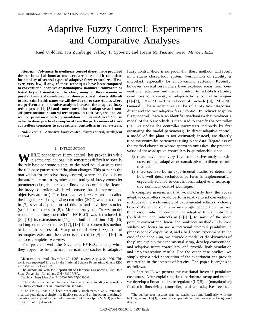
Fig. 1. Hardware setup of the inverted pendulum system.

linearizing controller (AFL). Next, we design two indirectadaptive fuzzy controllers, one that does not usea prioriinformation about the plant, and one that does. Followingthis, we specify two direct adaptive fuzzy controllers, onethat uses a feedback linearizing controller as the “knownpart” of the controller and another that uses an LQR forinitialization. Simulation and implementation results are shownin all cases. Finally, we summarize and discuss the results andthe performance of each controller.

In Section III, we present the process control case study.After providing the experimental setup and model we sum-marize our results using a feedback linearizing controller andan indirect adaptive fuzzy controller. In Section IV, we firstdescribe the ball-beam experiment and its mathematical model.Then we develop a (nonadaptive) fuzzy controller and a directadaptive fuzzy controller and compare their performance insimulation and implementation. In Section V, the concludingremarks, we summarize the overall results, provide a broadassessment of the apparent advantages and disadvantages ofthe adaptive fuzzy control techniques, and provide some futureresearch directions which help to identify limitations of thescope and content of this paper. This paper is a significantlyexpanded version of the one in [30].

II. ROTATIONAL INVERTED PENDULUM

In our first case study for indirect and direct adaptive fuzzycontrol, we will focus on a rotational inverted pendulum testbed. Since adaptive control is being studied, special emphasiswill be put on robustness by investigating the ability ofthe controllers to compensate for significant plant parametervariations.

A. Experiment Setup

The rotational inverted pendulum is an underactuated (i.e.,it has fewer inputs than degrees of freedom), unstable system

that presents considerable control-design challenges, and is,therefore, appropriate for testing the performance of differentcontrol techniques. The experimental setup used in this paperwas developed in [31] and [32], where a nonlinear mathe-matical model of the system was obtained via identificationtechniques, and four different control methods were applied:proportional derivative control, linear quadratic regulation,direct fuzzy control, and autotuned fuzzy control.

The hardware setup of the system is shown in Fig. 1 (takenfrom [31]). It consists of three principal parts: the pendulumitself (controlled object), interface circuits, and the controller,implemented by means of a program in a digital computer.The controller can actuate the pendulum by turning the dcmotor to which it is attached. The motor has an optical encoderon its shaft that allows the measurement of its angle (withrespect to the starting position) which we will refer to as.The shaft of the motor has a rotating base fixed to it. Thependulum can rotate freely around the base, and its angle,,can also be measured with an optical encoder with respect tothe pendulum’s stable equilibrium point, where it is assumedto have a value of radians. The input voltage to the dc motoramplifier is constrained to a range of5 V.

As detailed in [31], the rotational pendulum system presentstwo somewhat separate problems: first, a controller needsto be designed that is able to balance the pendulum, andsecond, an adequate algorithm has to be used to swing upthe pendulum so that when it reaches an upright position(i.e., where ) its angular velocity ( ) is close tozero. This facilitates the job of the controller which “catches”the pendulum and tries to balance it. In this paper, we willnot be concerned with swing-up details, and will concentrateonly on the balancing control of the pendulum. The so-called“simple energy pumping” swing-up algorithm developed in[31]4 will be used without changes in all the experiments and

4Please consult this reference for details on the swing-up algorithm.

ORDONEZ et al.: ADAPTIVE FUZZY CONTROL: EXPERIMENTS AND COMPARATIVE ANALYSES 169

simulations, only with minor tunings depending on the natureof the test. This algorithm is just a proportional controllerwhich takes as input the error between a maximum swingangle (the tuning parameter) and the base angle.

In implementation, a sampling time of 0.01 s was used.All the simulation and experimental plots include the swing-up phase and show the first 6 s only, since this time wasconsidered enough to show the representative aspects of theresults.

B. Modeling and Simulation

The rotational inverted pendulum can be represented with afour-state nonlinear model. The states are, , , and . Ofthem, only and are directly available for measurement;the other two states have to be estimated. To do this, weuse a first-order backward difference approximation of thederivative. As tested in [31], this estimation method turnsout to be very reliable and accurate. Thus, for the rest ofthe discussion, it will be assumed that all states are directlyavailable for the controllers without need of further estimation.

The differential equations that describe the dynamics of thependulum system (note that is the unstable equilibriumpoint) are given by

(1)

(2)

where Kg is the mass of the pendulum,m is the distance from the center of mass of

the pendulum, is the acceleration due togravity, is the inertia ofthe pendulum, rad is thefrictional constant between the pendulum and the rotating base,

is a proportionality constant, and isthe control input (voltage applied to the motor). A first-ordermodel of the dc motor is given bywith and . The numerical valuesof the constants were determined experimentally in [31]. Notethat the sign of depends on whether the pendulum is in theinverted or the noninverted position, i.e., forwe have , and otherwise(recall that is the stable equilibrium point). Whensimulating the system, a conditional statement is used todetermine the sign of according to the relation above.

Let , , , and . Then a statevariable representation of the plant is given by

(3)

where , , ,, , and . Since we

are only interested in balancing the pendulum, we take theoutput of the system as .

For simulation of the system, a fourth-order Runge–Kuttanumerical method was used in all cases, with an integration

step size of 0.001 s. The controllers are assumed to becontinuous; therefore, the sampling time of the controller wasset equal to the integration step size. Also, the initial conditionswere kept identical in all simulations; these are rad,

rad , rad, and rad . Underthese conditions, the pendulum is in the downward position.When the simulations start, the pendulum is first swung upwith the same swing-up algorithm used for implementation,and then “caught” by the balancing controller currently beingtested to resemble experimental conditions as accurately aspossible. The balancing controller begins to act when

rad; at the same time, the swing-up controller is shut down.For the swing-up algorithm, we have one design parameter,

the angle , with values typically between 1.1 and 1.4 radians;this angle determines the maximum amplitude of each swing.The gain is fixed at 0.75 for all tests. Then, taking asthe swing-up control input, the algorithm works as follows:

If then

else

C. Two Nonadaptive Controllers

In this section, two nonadaptive controllers for the invertedpendulum will be introduced, and these will serve as a baselinefor comparison to the results to follow. First, a linear quadraticregulator from [31] (which provided the best experimental re-sults for nominal conditions) will be used. Second, a feedbacklinearizing control law will be used; as shown later, there is noguarantee of boundedness using this technique, and the resultsobtained here corroborate this theoretical prediction.

1) Linear Quadratic Regulator:To design an LQR for thependulum, the approach taken in [31] was to linearize thesystem model by using the approximation , whichis valid for small angles, in (3). The resulting system can beshown to be controllable; thus, an LQR can be constructed.For the design, the greatest penalty was assigned to theerror in states and , since the primary objective of thecontroller is to balance the pendulum, and not to keep the basefrom moving. The state-feedback gain obtained was testedexperimentally and, after some fine tuning, the gain vectorused was , where the state error

( is a reference-state trajectory, typically setidentically equal to zero) is used, and .

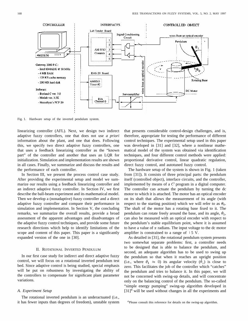
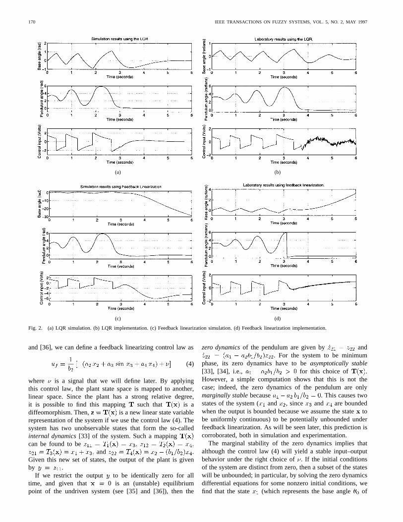
As shown in Fig. 2(a) and (b), the LQR performs verywell in both simulation and implementation; it successfullybalances the pendulum and drives all the system states to zero.The control input ideally goes to zero when equilibrium isreached [Fig. 2(a)], although in practice it does not [Fig. 2(b)],since the unmodeled aspects of the system (e.g., sensor noise,sampling time, nonlinear characteristics, etc.) prevent thecontroller from behaving perfectly. The results obtained hereclosely match those in [31].

2) Feedback Linearizing Controller:We find that the in-verted pendulum has astrong relative degree[33], [34] oftwo because after differentiating the output twice, we obtain

. Then, as described in [35]


(a) (b)

(c) (d)

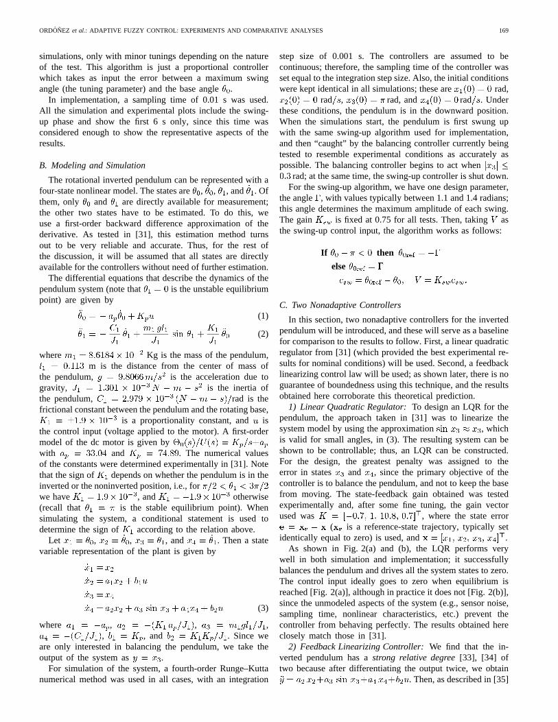
Fig. 2. (a) LQR simulation. (b) LQR implementation. (c) Feedback linearization simulation. (d) Feedback linearization implementation.

and [36], we can define a feedback linearizing control law as

(4)

where is a signal that we will define later. By applyingthis control law, the plant state space is mapped to another,linear space. Since the plant has a strong relative degree,it is possible to find this mapping such that is adiffeomorphism. Then, is a new linear state variablerepresentation of the system if we use the control law (4). Thesystem has two unobservable states that form the so-calledinternal dynamics[33] of the system. Such a mappingcan be found to be

and .Given this new set of states, the output of the plant is givenby .

If we restrict the output to be identically zero for alltime, and given that 0 is an (unstable) equilibriumpoint of the undriven system (see [35] and [36]), then the

zero dynamicsof the pendulum are given by and. For the system to be minimum

phase, its zero dynamics have to beasymptotically stable[33], [34], i.e., for this choice of .However, a simple computation shows that this is not thecase; indeed, the zero dynamics of the pendulum are onlymarginally stablebecause . This causes twostates of the system ( and , since and are boundedwhen the output is bounded because we assume the statetobe uniformly continuous) to be potentially unbounded underfeedback linearization. As will be seen later, this prediction iscorroborated, both in simulation and experimentation.

The marginal stability of the zero dynamics implies thatalthough the control law (4) will yield a stable input–outputbehavior under the right choice of. If the initial conditionsof the system are distinct from zero, then a subset of the stateswill be unbounded; in particular, by solving the zero dynamicsdifferential equations for some nonzero initial conditions, wefind that the state (which represents the base angleof


the rotational pendulum) will be given by in steadystate, where represents time andis an integration constant.

It is worth noting that the unboundedness of can betolerated in this experiment, since all it means is that thependulum base keeps rotating while the pendulum is beingbalanced. Of course, in practice, a limit is imposed on therate and amount of this rotation to protect the machinery, butin principle, the marginal stability of the zero dynamics caneffectively be dealt with.

To simulate and implement the feedback linearizing closedloop, it is necessary to specify the signal. Let bea prespecified reference trajectory (set equal to zero for allcases in this work), at least twice differentiable, and take

(following the notation in [35] and [36]).Then, let with which we obtain astable (in the input–output sense) closed-loop system withpoles at . This choice of the closed-loop poleswas made because of practical considerations: experience withfeedback linearization on the pendulum experiment indicatesthat attempting to bring the output error to zero too fastcan sometimes result in failure or a degraded performance;therefore, these somewhat slow poles were chosen.

The simulation results in Fig. 2(c) are as expected—thependulum is balanced, and the base keeps rotating at an almostconstant velocity. Note that this controller settles the controlinput at a nonzero value, which in turn introduces energy intothe system and causes its base to rotate; this is easily explainedby the theoretical analysis of the zero dynamics. A comparisonwith the experimental results in Fig. 2(d) shows significantsimilarities: after the swing-up phase, the statesand , aswell as the control input, behave as in the simulation. Observethat in simulation the feedback linearizing controller reachesa peak value of 6 V to balance the pendulum; althoughin implementation the control input is limited to 5 V asexplained above, no such bound was used for simulation sincewe desired to preserve ideal circumstances regarding controlaction.

D. Adaptive Feedback Linearization

Both the feedback linearizing controller and the LQR, aswell as almost any other nonadaptive technique used on thependulum fail (or in the case of direct fuzzy control havedegraded performance [31]) when the nominal system (i.e., thependulum without any mass changes or added disturbances)is altered in anunknown way. It is in such a situation thatadaptive control plays a central role since it is, at least inprinciple, able to deal with significant plant changes. In thisinvestigation, two types of plant alterations were used—acontainer half filled with metal bolts fixed at the tip of thependulum, and a container half filled with water fixed at thetip of the pendulum.

The added weight (not accounted for in the design of thecontrollers) not only shifts the pendulum’s center of mass awayfrom the pivot point (which, in turn, decreases the naturalfrequency of the pendulum) and makes the effects of frictionless dominant, but also introduces random disturbances thatvary in nature with the bolts and the water. In the case of the

water container, a “sloshing liquid” effect is created, whichstrongly affects the dynamics of the system. As will be seenfrom the results below, the bolts have a different type of effectthat is caused by their “rattling” during balancing.

We note that the adaptive controllers in this subsection andthe remainder of this section are based on the assumption thatthe plant is minimum-phase (see [3], [36]). Since this assump-tion does not hold for the pendulum, some consequences of thetechniques are no longer guaranteed; specifically, we shouldnot expect the state (and possibly the control input) tobe bounded, because its behavior will depend on the initialconditions of the system. However, the study of the adaptivetechniques on such a system is of theoretical and practical rel-evance because, in the first place, it provides a good exampleof practical results very well predicted by theoretical analysisof nonlinear systems, and in the second place, it can giveinsight into how to overcome the limitations of the adaptivecontrollers inherited by their underlying assumptions. As willbe shown, it is indeed possible to obtain not only stability andboundedness, but also good robustness to unmodeled plantchanges.

The adaptive fuzzy techniques illustrated in this paper arebased on feedback linearization; therefore, adaptive feedbacklinearization (AFL) seemed the most natural choice for refer-ence and comparison to conventional adaptive control. For thedesign of this controller, the technique described in [35] and[36] was used as we discuss next.

We first rewrite (3) as a linear combination of known, fixed,nonlinear functions

(5)

where

(6)

We shallestimate and by searching for the optimumvectors and .We use and to denote the estimates of theoptimum parameter vectors at time. Then, the adaptivecontrol law is given bywhere stands for the estimated Lie derivative ofwithrespect to , as defined in [34] and [36], and the variablehas been dropped for convenience. To allow for tracking, wetake , with and

to have the same poles as in the nonadaptive feedback


linearization. Notice that does not need to be estimated, sincehas already been approximated by a backward

difference, as explained above.Following [35], define as a vector contain-

ing all the combinations , , , and

. For adaptation, define an error signal of theform with , where the transferfunction is strictly positive real [33].The adaptation law given by a normalized gradient approach is

(7)

where is the regressorvector obtained by computing theoutput error equation (see [36]). To startthe search for the optimum vectors and at thebest known point in the search space, their estimatesand were initialized using the parameters obtainedfrom the system model, and

. For simulation and implementation weused and . These values for andwere determined via manual tuning; after several simulationand experimentation trials, they were the choices that, as faras we could determine, made the controller work at its bestand still maintain the strictly positive real condition.

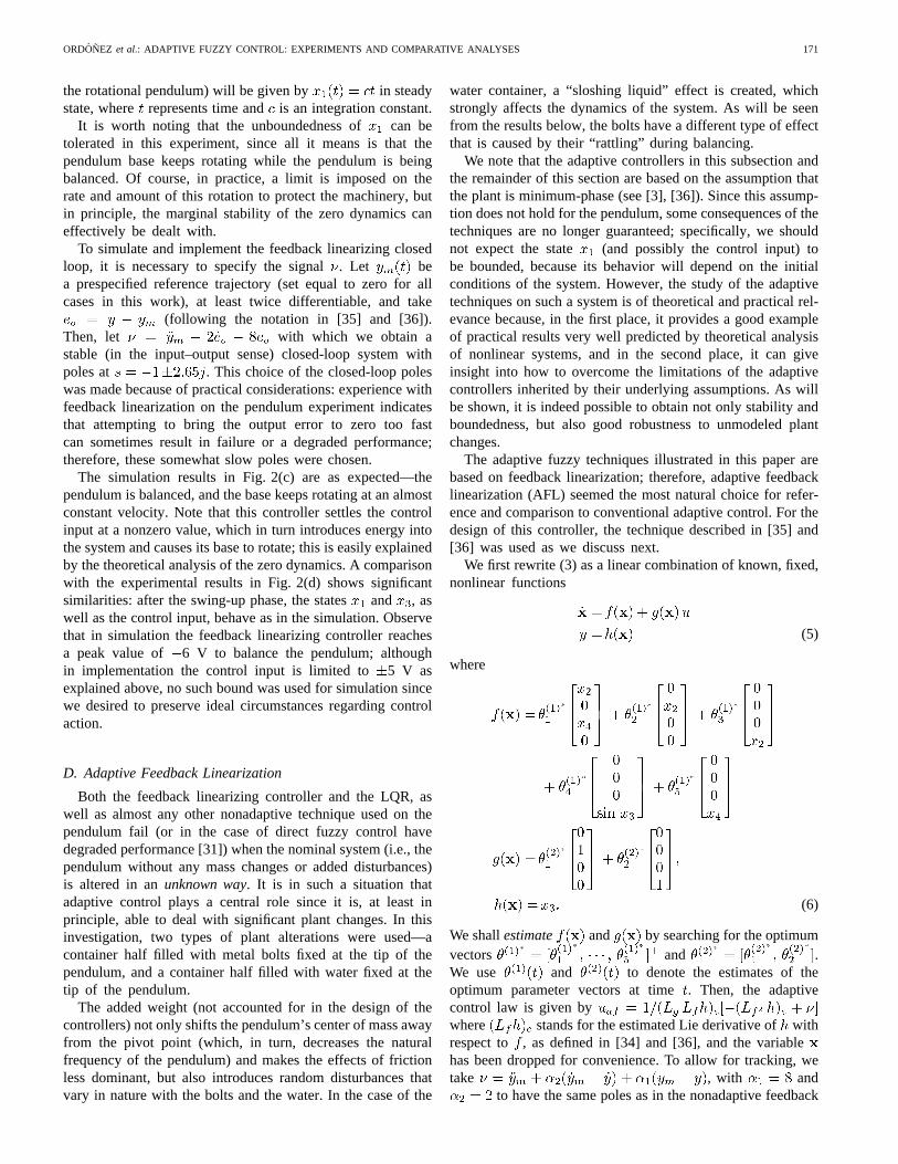
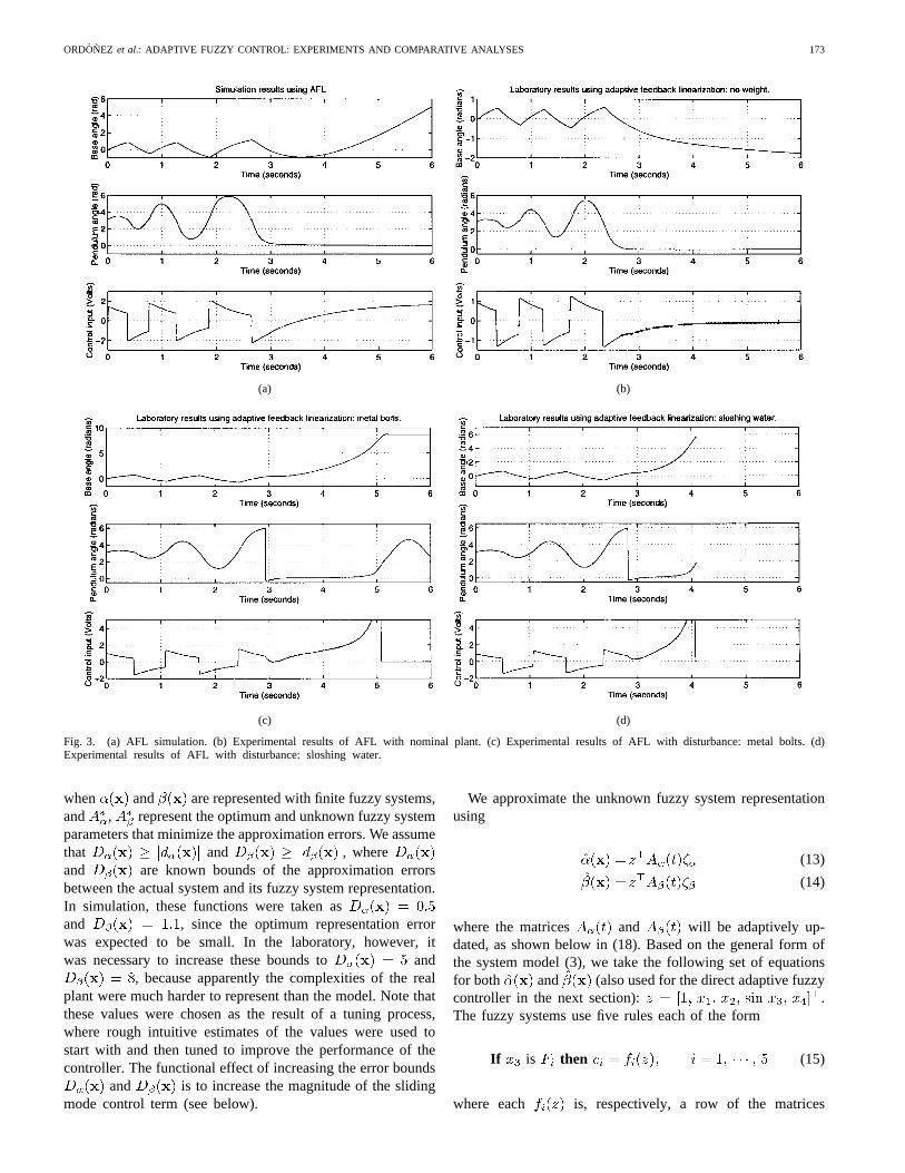
Fig. 3 contains the results obtained with AFL. Fig. 3(a) hascharacteristics similar to those of the nonadaptive feedbacklinearization in Fig. 2(a), although the required control inputstays within implementation bounds. For the nominal plant, thecontroller exhibits very good behavior, as seen in Fig. 3(b):the pendulum is perfectly balanced and the control inputsettles at a value close to zero so the base rotates slowly.In Fig. 3(c) we observe that the controller manages to balancethe pendulum with bolts, but only for a short time; the base isturning rapidly and, at about the fifth second, the control inputreaches the its limit of 5 V. The controller had the greatestproblems with water and was not able to maintain equilibrium,as seen in Fig. 3(d). In the next section, we will show how theadaptive fuzzy control techniques can significantly outperformthis conventional adaptive controller.

E. Indirect Adaptive Fuzzy Control

Here, an indirect adaptive fuzzy controller (IAFC) will bedeveloped for the inverted pendulum; two possible configu-rations will be presented and used for experiments. First, acontroller that does not make an explicit use of the knownplant dynamics to estimate the “certainty equivalence controlterm” [1], [3] will be used on the pendulum. Second, it willbe illustrated how to incorporate the knowledge of the model(3) in the design. It will be shown experimentally that suchan enhanced controller has, in the case of the pendulum, a no-ticeable advantage over the previous techniques, and providesan increased robustness against the induced disturbances.

For what follows in this section and the next, the notationfrom [1]–[3] will be used. Moreover, in the interest of beingbrief, we do not repeat the theoretical development of the con-trollers in [1]–[3], and simply provide a complete descriptionof each controller. To fully understand why the controllers in

this and the next section result in stable operation, the readershould consult [1]–[3].

1) Design without Use of Plant Dynamics Knowledge:Aspreviously shown, the pendulum model has a relative degreeof two. The input–output differential equation of the pendulummodel can thus be rewritten as

(8)

where, for now, we take and ( andare known, measurable parts of the dynamics [3]), and

substituting the numerical values of the parameters we obtain

(9)

(10)

In these equations, we use “approximately equal” signs be-cause the numerical parameters of the equations are notexpected to represent the pendulum’s input–output dynamicsexactly; rather, the right-hand side of (9) and (10) are simplyourbest known approximationsto and , respectively.Note that , so there exists a (take, for instance,

, which gives us a safe margin of error) such thatfor all ; thus, is bounded away from

zero, a condition we will need to ensure stability.It is possible to represent (9) and (10) using a special

form of Takagi–Sugeno fuzzy systems [37]. To briefly presentthe notation, take a fuzzy system denoted by . Then,

. Here, singleton fuzzificationof the input is assumed; the fuzzy systemhas rules, and is the value of the membership functionfor the antecedent of theth rule given the input . It isassumed that the fuzzy system is constructed in such a waythat for all . The parameter isthe consequent of theth rule which, in this paper, will betaken as a linear combination of Lipschitz continuous functions

, , so that, . Define

...

......

......

Then, the nonlinear equation that describes the fuzzy systemcan be written as (notice that standard fuzzysystems may be treated as special cases of this more generalrepresentation [3]).

Given this notation, we can write

(11)

(12)

where , are the approximation errors that arise


(a) (b)

(c) (d)

Fig. 3. (a) AFL simulation. (b) Experimental results of AFL with nominal plant. (c) Experimental results of AFL with disturbance: metal bolts. (d)Experimental results of AFL with disturbance: sloshing water.

when and are represented with finite fuzzy systems,and , represent the optimum and unknown fuzzy systemparameters that minimize the approximation errors. We assumethat and , whereand are known bounds of the approximation errorsbetween the actual system and its fuzzy system representation.In simulation, these functions were taken asand , since the optimum representation errorwas expected to be small. In the laboratory, however, itwas necessary to increase these bounds to and

, because apparently the complexities of the realplant were much harder to represent than the model. Note thatthese values were chosen as the result of a tuning process,where rough intuitive estimates of the values were used tostart with and then tuned to improve the performance of thecontroller. The functional effect of increasing the error bounds

and is to increase the magnitude of the slidingmode control term (see below).

We approximate the unknown fuzzy system representationusing

(13)

(14)

where the matrices and will be adaptively up-dated, as shown below in (18). Based on the general form ofthe system model (3), we take the following set of equationsfor both and (also used for the direct adaptive fuzzycontroller in the next section): .The fuzzy systems use five rules each of the form

If is then (15)

where each is, respectively, a row of the matrices


Fig. 4. Input membership functions.

and , and we initialize the system with

(16)

Note that this fuzzy system design is overspecified, mainly inthe case of because, from the system model, this functionis not expected to depend on the state vector. However, thischoice was made to allow for a greater adaptation flexibility.The initialization (16) gives the system the best-known startingpoint in the search space. The input fuzzy setsare asdescribed in Fig. 4 (the normalizing gain for the input to thefuzzy system was set to one for simplicity).

Define the signals and, where now we take and we let ,

(with these choices, the poles of the error transferfunction are at and , which produce a smallerror settling time). Then, the indirect adaptive control law[1], [3] is given by

(17)

where thecertainty equivalence control termis taken as. The sliding-mode control termis

given by sgn . Todefine thebounding control term , we first need to determinebounding functions and for and ,respectively. Based on the numerical values of (9) and (10),the bounding functions were empirically determined to be

, . Then, let

sgn whenever , and otherwise.The parameter defines a bounded, closed subset of the

error-state space within which the error is guaranteed tostay. For simulation, we took ; again, a largermargin had to be used in implementation, and the smallestacceptable value was . Note that although it is possible,in principle, to take an arbitrarily small , in practice it isoften the case that the bounding control acts “too much” witha small , and the unavoidable limits in the control-inputsignal cause the system to become unstable. Also note thatfrom the stability analysis in [1] and [3], the bounding controlterm is not required for stability and may, thus, beset to zero

if it provides no advantage in a particular design. However,it gives the designer the flexibility of choosing a hard boundfor the tracking error, which in the case of the pendulum isa useful feature.

To define the adaptation equations, letbe a identitymatrix, and let for simulation, andfor implementation, and take

(18)

A projection algorithm is used to ensure that andremain within reasonable limits; specifically, it is sufficient toensure that is bounded away from zero with

.Note that the IAFC adaptation algorithm guarantees that the

parameter error matrices andwill at least stay bounded. Note also that (9) and

(10) are themselves only approximations, based on our bestknowledge of the plant. Thus, it is possible that the fuzzysystem representation of the input–output equation and

does not converge to (9) and (10), but perhaps to a better(or worse) model of the system.

In this way, the IAFC from [1] and [3] is completelyspecified. One of its assumptions is not satisfied, namely, thatthe zero-dynamics of the plant are exponentially attractive;thus, as happened with the adaptive and nonadaptive feed-back linearizing controllers, boundedness of the state, andpossibly of the control input , is not expected. However,in principle, the controller should be able to achieve outputconvergence (i.e., keep the pendulum balanced).

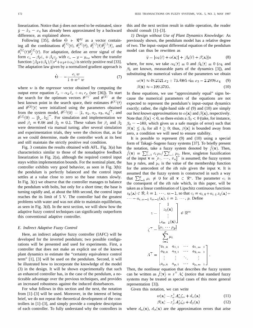
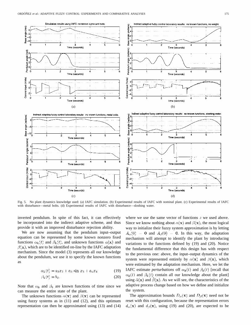
We see in Fig. 5(a) that this is indeed the case. Thependulum is successfully balanced, and the settling time of thecontroller is smaller than in the case of any of the previouscontrollers since here , which haspoles at and ; the reason why this signalwas not used for the (adaptive and nonadaptive) feedbacklinearizing controllers is that with it they performed worse,both in simulation and experimentation, in terms of errorconvergence and robustness.

For implementation, we see in Fig. 5(b) that the pendulumis balanced using the nominal plant, although the outputerror is not exactly zero. When the bolts disturbance is used[Fig. 5(c)], the controller has trouble similar to AFL [seeFig. 3(c)] because the control input reaches its lower limitof 5 V. We see in Fig. 5(d) that with sloshing water,the controller performs better, although it is apparent thatthe control input limit is about to be reached. Thus, theperformance of this IAFC design is roughly similar to thatof adaptive feedback linearization.

2) Incorporation of Plant Dynamics Knowledge in Design:To improve the robustness characteristics of the IAFC, wewill now take a slightly different design approach and willmake explicit and direct use of the knowledge we have ofthe plant, i.e., the nonlinear model (3). By comparing thesimulation and experimental results so far, we see that althoughvery useful for theoretical analysis and design, the model isnevertheless a relatively poor approximation of the rotational


(a) (b)

(c) (d)

Fig. 5. No plant dynamics knowledge used: (a) IAFC simulation. (b) Experimental results of IAFC with nominal plant. (c) Experimental results of IAFCwith disturbance—metal bolts. (d) Experimental results of IAFC with disturbance—sloshing water.

inverted pendulum. In spite of this fact, it can effectivelybe incorporated into the indirect adaptive scheme, and thusprovide it with an improved disturbance rejection ability.

We are now assuming that the pendulum input–outputequation can be represented by some known nonzero fixedfunctions and , and unknown functions and

, which are to be identified on-line by the IAFC adaptationmechanism. Since the model (3) represents all our knowledgeabout the pendulum, we use it to specify the known functionsas

(19)

(20)

Note that and are known functions of time since wecan measure the entire state of the plant.

The unknown functions and can be representedusing fuzzy systems as in (11) and (12), and this optimumrepresentation can then be approximated using (13) and (14)

where we use the same vector of functionswe used above.Since we know nothing about and , the most logicalway to initialize their fuzzy system approximation is by letting

and . In this way, the adaptationmechanism will attempt to identify the plant by introducingvariations to the functions defined by (19) and (20). Noticethe fundamental difference that this design has with respectto the previous one: above, the input–output dynamics of thesystem were represented entirely by and , whichwere estimated by the adaptation mechanism. Here, we let theIAFC estimateperturbationsoff and [recall that

and contain all our knowledge about the plant]using and . As we will see, the characteristics of theadaptive process change based on how we define and initializethe system.

The approximation bounds and need not bereset with this configuration, because the representation errors

and , using (19) and (20), are expected to be


(a) (b)

(c) (d)

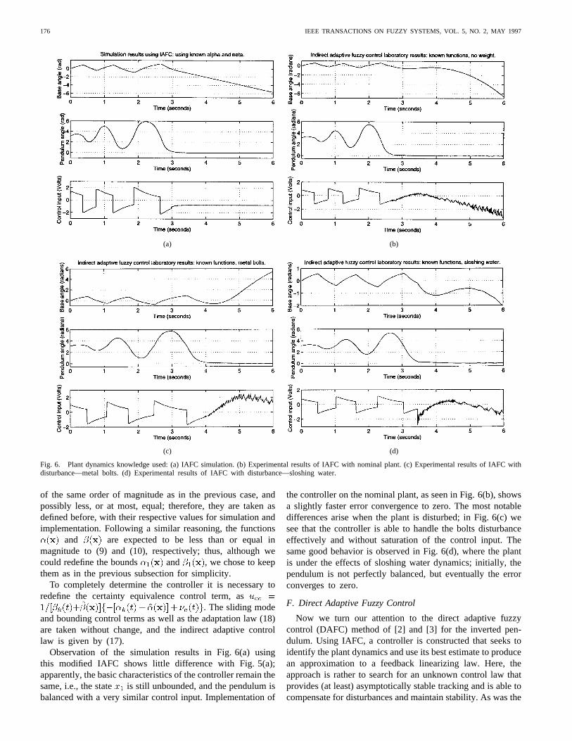
Fig. 6. Plant dynamics knowledge used: (a) IAFC simulation. (b) Experimental results of IAFC with nominal plant. (c) Experimental results of IAFC withdisturbance—metal bolts. (d) Experimental results of IAFC with disturbance—sloshing water.

of the same order of magnitude as in the previous case, andpossibly less, or at most, equal; therefore, they are taken asdefined before, with their respective values for simulation andimplementation. Following a similar reasoning, the functions

and are expected to be less than or equal inmagnitude to (9) and (10), respectively; thus, although wecould redefine the bounds and , we chose to keepthem as in the previous subsection for simplicity.

To completely determine the controller it is necessary toredefine the certainty equivalence control term, as

. The sliding modeand bounding control terms as well as the adaptation law (18)are taken without change, and the indirect adaptive controllaw is given by (17).

Observation of the simulation results in Fig. 6(a) usingthis modified IAFC shows little difference with Fig. 5(a);apparently, the basic characteristics of the controller remain thesame, i.e., the state is still unbounded, and the pendulum isbalanced with a very similar control input. Implementation of

the controller on the nominal plant, as seen in Fig. 6(b), showsa slightly faster error convergence to zero. The most notabledifferences arise when the plant is disturbed; in Fig. 6(c) wesee that the controller is able to handle the bolts disturbanceeffectively and without saturation of the control input. Thesame good behavior is observed in Fig. 6(d), where the plantis under the effects of sloshing water dynamics; initially, thependulum is not perfectly balanced, but eventually the errorconverges to zero.

F. Direct Adaptive Fuzzy Control

Now we turn our attention to the direct adaptive fuzzycontrol (DAFC) method of [2] and [3] for the inverted pen-dulum. Using IAFC, a controller is constructed that seeks toidentify the plant dynamics and use its best estimate to producean approximation to a feedback linearizing law. Here, theapproach is rather to search for an unknown control law thatprovides (at least) asymptotically stable tracking and is able tocompensate for disturbances and maintain stability. As was the


case with IAFC, the DAFC methodology allows the designer touse previous knowledge or experience with the plant in variousways. Here, we will illustrate two representative possibilities,and we will see that is possible to obtain significantly differentcontrol results depending on the approach taken.

In IAFC, it was possible to use a known part of the plantdynamics represented by and in the control design.We saw that for the pendulum application it was beneficialto include the known dynamics because it increased therobustness of the design. DAFC provides the designer witha method to incorporate a best guess of what the controllershould be (below we will call this the “known controller,”denoted by ). The algorithm then adaptively tunes a fuzzycontroller to compensate for inaccuracies in our choice of thisknown controller.

1) Design Using Feedback Linearization as a Known Con-troller: As described in [2] and [3], DAFC is a somewhatmore restrictive technique than its indirect counterpart since,in addition to the assumption that the plant is minimum-phase,it is also required that the system input–output (8) is such that

for ; further, it is assumed that is boundedby two finite constants, and . For the pendulum, thisassumption holds since , where,for instance, we take, as before, and .The last plant assumption needed in [2] and [3] is that forsome , . Since is expected to bea constant, we can safely set , and the assumptionholds.

Note that the control equations derived in [2] and [3]are based on the premise that is positive, but it isstated there that the laws can be modified to allow for thenegative case. Thus, the equations used here will be slightlymodified versions of those in [2] and [3], as required by thecharacteristics of the pendulum; specifically, the adaptationdifferential equation and the sliding-mode control term willeach have a small but crucial sign change.

Let be an unknown ideal controller that we will try to ap-proximate. In [2] and [3], this ideal controller is assumed to bea feedback linearizing law of the form

In general, it is possible to express in terms of aTakagi–Sugeno fuzzy system, aswhere is some known controller term, which we will usein this section and set equal to zero in the next, andis the error between the fuzzy representation and. It isassumed that , where is a knownbound for the error. In practice, it is often hard to have aconcrete idea about the magnitude of , because therelation between and its fuzzy representation might bedifficult to characterize; however, it is much easier to beginwith a rough, intuitive idea about this bound, and then iteratethe design process and adjust it, until the performance of thecontroller indicates that one is close to the right value. Forsimulation, we found that gave us good results,and in the laboratory, we increased it to . Thesebounds are both relatively small, which indicates that the fuzzysystem we used, although a simple one, could represent theideal controller with sufficient accuracy.

We are going to search for using

(21)

where is as defined for the IAFC, with the fuzzy setsof Fig. 4. The matrix is adaptively updated on-line, and the function vector is taken as in the previousSection. The fuzzy system again uses only five rules, asgiven by (15), and now each is a row of the matrix

. To approximate a feedback linearizing controllerwe will define as in law (4), and we will take as inthe feedback linearization design. Further, following the sameline of thought as in Section II-E.2, we initialize the fuzzysystem with .

The DAFC control law is given by .It is formed by three terms: the fuzzy approximation to theoptimum controller (21), and sliding and bounding controlterms. Take the signals and as defined for the IAFCcase. Since (as noted above) , the sliding-modeterm is given by sgn . Note the minussign which is a result of the fact that .

The bounding-control term needs the assumption thatis bounded, with . We take as de-fined before; then, if ,

sgn and otherwise.For simulation, we used and increased it to

in implementation. Please refer to the discussion onIAFC for an explanation on how we determined these values.

The last part of the DAFC mechanism is the adaptation law,which is chosen in such a way that the output error convergesasymptotically to zero, and the parameter error remains at leastbounded. This law is given, in general, by

(22)

Again, note the minus sign for . The parameter canbe chosen nonzero to potentially improve adaptation [2], [3],but here we took for . For simulation, weused , and in experimentation we decreased thegain slightly to . With these choices the algorithmwas able to adapt and estimate the control lawfast enoughto perform well and compensate for disturbances, but withoutinducing oscillations typical of a too high adaptation rate.

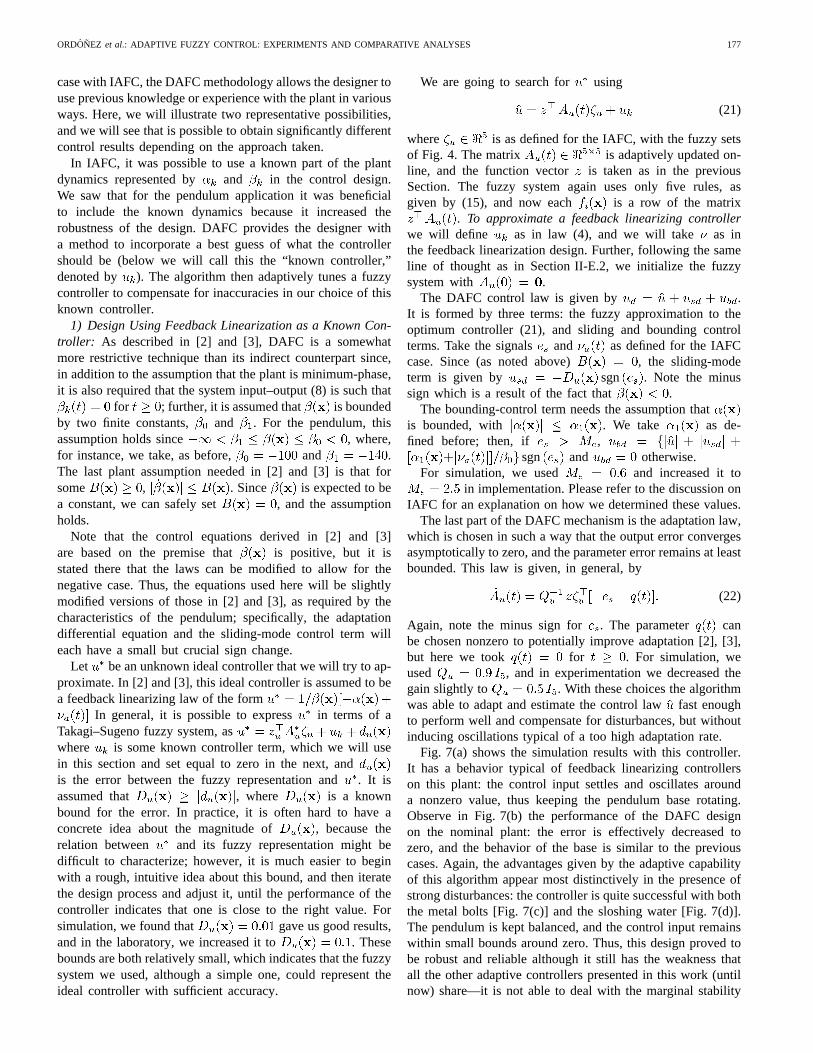
Fig. 7(a) shows the simulation results with this controller.It has a behavior typical of feedback linearizing controllerson this plant: the control input settles and oscillates arounda nonzero value, thus keeping the pendulum base rotating.Observe in Fig. 7(b) the performance of the DAFC designon the nominal plant: the error is effectively decreased tozero, and the behavior of the base is similar to the previouscases. Again, the advantages given by the adaptive capabilityof this algorithm appear most distinctively in the presence ofstrong disturbances: the controller is quite successful with boththe metal bolts [Fig. 7(c)] and the sloshing water [Fig. 7(d)].The pendulum is kept balanced, and the control input remainswithin small bounds around zero. Thus, this design proved tobe robust and reliable although it still has the weakness thatall the other adaptive controllers presented in this work (untilnow) share—it is not able to deal with the marginal stability


(a) (b)

(c) (d)

Fig. 7. DAFC using feedback linearizinguk. (a) DAFC simulation. (b) Experimental results of DAFC with nominal plant. (c) Experimental results of DAFCwith disturbance—metal bolts. (d) Experimental results of DAFC with disturbance—sloshing water.

condition of the system’s zero dynamics. Therefore, as a lastand, in our opinion, best fuzzy adaptive design example, wewill now describe a DAFC that cannot only compensate forthe induced disturbances (and, in fact, it does it with greaterease than all the previous controllers), but is also able to keepstate boundedness, even though the theoretical analysis of [2]and [3] does not predict it (recall that such analysis does notpreclude it).

2) Using the LQR to Obtain Boundedness:Although thetheoretical analysis in [2] and [3] uses the assumption that theunknown control law , which the DAFC tries to identify asa feedback linearizing law, it was found experimentally that itis not necessarily the case. If the right known controller is usedand/or the adaptation mechanism is initialized appropriately,then the adaptation algorithm will converge to a controllerthat might behave in a very different manner because thismechanism seems to try to find the (local) optimum controllerclosest to its starting point in the search space, and this

optimum does not necessarily have to be a feedback linearizingcontroller.

This finding is of special importance when the controldesign task involves dealing with a nonminimum phase plantlike the pendulum, for which feedback linearization-basedadaptive techniques have the limitation of being unable tomaintain complete state boundedness. As stated before, theunboundedness of the state is admissible for the pendulum,but it might not be for other systems.

Consider, for instance, that a nonadaptive controller isavailable that can control the nonminimum phase plant withstate boundedness. Then, it is possible that the desirableboundedness characteristics of this controller can be incorpo-rated into the DAFC design, and enhanced by the robustnessthat the adaptive method provides. It is not yet known howto characterize, in general, the controllers that can be used insuch a way; however, for our present study, a most natural andintuitive choice for this purpose is the LQR. This controller


implements a linear function of the plant states, and is, there-fore, able to drive the state error to zero for the nominal plantwhile maintaining state boundedness. Observe in Fig. 2(a) and(b) that all the plant states are indeed kept bounded. The LQRwas shown to have a very good performance on the nominal,undisturbed system. Nevertheless, it fails immediately whensignificant disturbances are introduced.

A DAFC will be designed based on the LQR, so that itsgood behavior in terms of state boundedness can be kept,and its weakness regarding plant disturbances eliminated.Two different, and functionally equivalent ways were foundto accomplish this. The first makes use of the term, asillustrated above. The second uses an appropriate initializationof the matrix . Since the use of has already been shown,only the second approach will be described here.

Again, take the control law defined above. The boundingand sliding-mode control terms are taken without changes.Also, the adaptation law (22) is used, now with a smaller gain(i.e., we slow adaptation down), , for simulationand implementation purposes. This adaptation gain was chosenvia tuning of the controller. We found that higher gains tendedto produce a more oscillatory behavior.

The fundamental difference between this and the previousdesign lies in the ideal that we aim to identify. Before,the adaptive search was configured in such a way that themechanism converged to a feedback linearizing law; now, wewant it to identify a control input that behaves basically like anLQR, i.e., we want to implement anadaptive LQR. To do this,it is necessary to start the adaptation algorithm at a point in thesearch space in the proximity of the ideal LQR controller.The closest approximation we have to this idealis the statefeedback gain vector of the LQR controller. Therefore, wewill use it to initialize the fuzzy approximation of the desiredcontrol . Take the fuzzy system described by (21), with thesame functions vector as before, and let . Then weinitialize the matrix as

(23)

Notice that the sign of the gains has been reversed since in thiscase we do not use the state error , but rather the vector,which consists of functions of the states themselves. It is worthmentioning that an alternative similar way of implementingthis design consists of using the control term (i.e.,we set equal to the LQR state feedback law) and letting

. We have tested this approach and it also worksvery well.

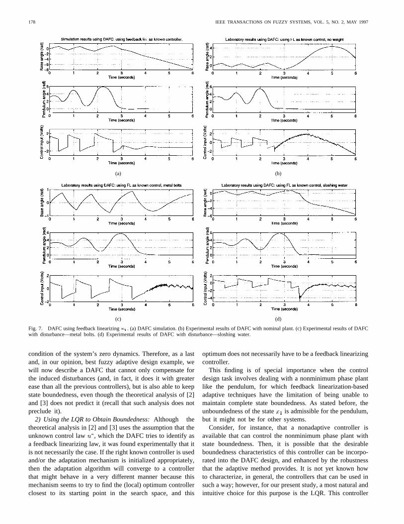
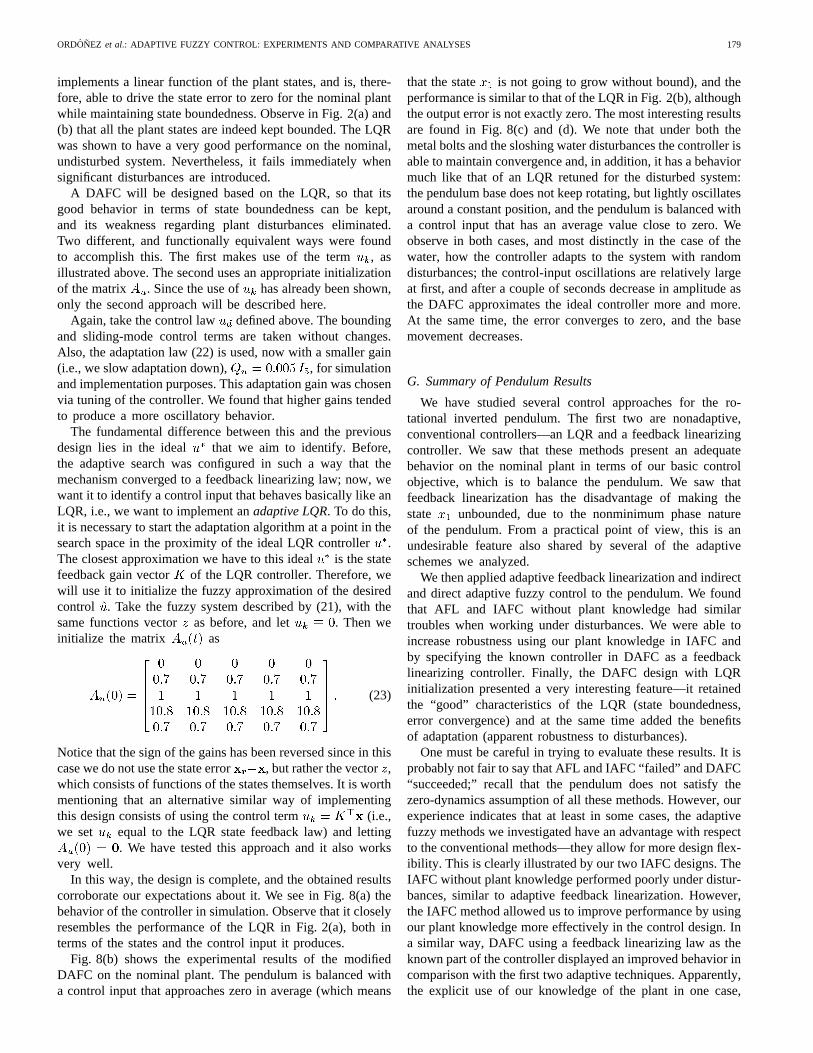
In this way, the design is complete, and the obtained resultscorroborate our expectations about it. We see in Fig. 8(a) thebehavior of the controller in simulation. Observe that it closelyresembles the performance of the LQR in Fig. 2(a), both interms of the states and the control input it produces.

Fig. 8(b) shows the experimental results of the modifiedDAFC on the nominal plant. The pendulum is balanced witha control input that approaches zero in average (which means

that the state is not going to grow without bound), and theperformance is similar to that of the LQR in Fig. 2(b), althoughthe output error is not exactly zero. The most interesting resultsare found in Fig. 8(c) and (d). We note that under both themetal bolts and the sloshing water disturbances the controller isable to maintain convergence and, in addition, it has a behaviormuch like that of an LQR retuned for the disturbed system:the pendulum base does not keep rotating, but lightly oscillatesaround a constant position, and the pendulum is balanced witha control input that has an average value close to zero. Weobserve in both cases, and most distinctly in the case of thewater, how the controller adapts to the system with randomdisturbances; the control-input oscillations are relatively largeat first, and after a couple of seconds decrease in amplitude asthe DAFC approximates the ideal controller more and more.At the same time, the error converges to zero, and the basemovement decreases.

G. Summary of Pendulum Results

We have studied several control approaches for the ro-tational inverted pendulum. The first two are nonadaptive,conventional controllers—an LQR and a feedback linearizingcontroller. We saw that these methods present an adequatebehavior on the nominal plant in terms of our basic controlobjective, which is to balance the pendulum. We saw thatfeedback linearization has the disadvantage of making thestate unbounded, due to the nonminimum phase natureof the pendulum. From a practical point of view, this is anundesirable feature also shared by several of the adaptiveschemes we analyzed.

We then applied adaptive feedback linearization and indirectand direct adaptive fuzzy control to the pendulum. We foundthat AFL and IAFC without plant knowledge had similartroubles when working under disturbances. We were able toincrease robustness using our plant knowledge in IAFC andby specifying the known controller in DAFC as a feedbacklinearizing controller. Finally, the DAFC design with LQRinitialization presented a very interesting feature—it retainedthe “good” characteristics of the LQR (state boundedness,error convergence) and at the same time added the benefitsof adaptation (apparent robustness to disturbances).

One must be careful in trying to evaluate these results. It isprobably not fair to say that AFL and IAFC “failed” and DAFC“succeeded;” recall that the pendulum does not satisfy thezero-dynamics assumption of all these methods. However, ourexperience indicates that at least in some cases, the adaptivefuzzy methods we investigated have an advantage with respectto the conventional methods—they allow for more design flex-ibility. This is clearly illustrated by our two IAFC designs. TheIAFC without plant knowledge performed poorly under distur-bances, similar to adaptive feedback linearization. However,the IAFC method allowed us to improve performance by usingour plant knowledge more effectively in the control design. Ina similar way, DAFC using a feedback linearizing law as theknown part of the controller displayed an improved behavior incomparison with the first two adaptive techniques. Apparently,the explicit use of our knowledge of the plant in one case,


(a) (b)

(c) (d)

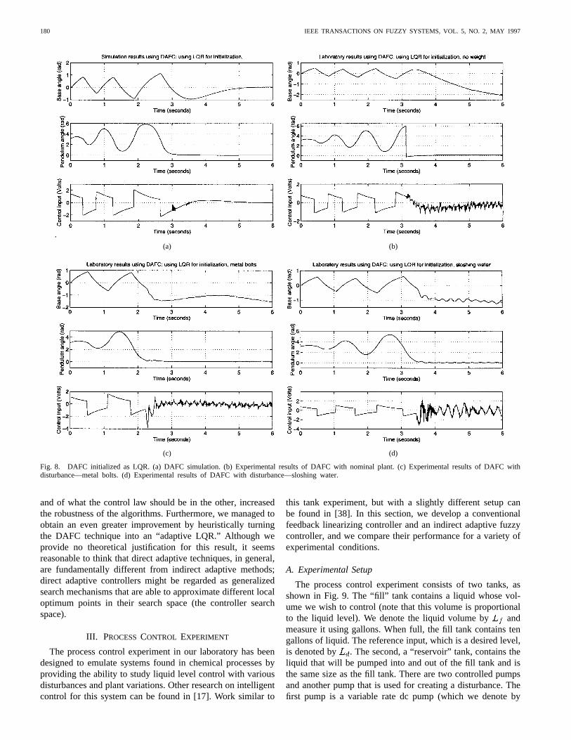
Fig. 8. DAFC initialized as LQR. (a) DAFC simulation. (b) Experimental results of DAFC with nominal plant. (c) Experimental results of DAFC withdisturbance—metal bolts. (d) Experimental results of DAFC with disturbance—sloshing water.

and of what the control law should be in the other, increasedthe robustness of the algorithms. Furthermore, we managed toobtain an even greater improvement by heuristically turningthe DAFC technique into an “adaptive LQR.” Although weprovide no theoretical justification for this result, it seemsreasonable to think that direct adaptive techniques, in general,are fundamentally different from indirect adaptive methods;direct adaptive controllers might be regarded as generalizedsearch mechanisms that are able to approximate different localoptimum points in their search space (the controller searchspace).

III. PROCESSCONTROL EXPERIMENT

The process control experiment in our laboratory has beendesigned to emulate systems found in chemical processes byproviding the ability to study liquid level control with variousdisturbances and plant variations. Other research on intelligentcontrol for this system can be found in [17]. Work similar to

this tank experiment, but with a slightly different setup canbe found in [38]. In this section, we develop a conventionalfeedback linearizing controller and an indirect adaptive fuzzycontroller, and we compare their performance for a variety ofexperimental conditions.

A. Experimental Setup

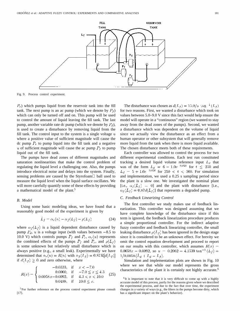
The process control experiment consists of two tanks, asshown in Fig. 9. The “fill” tank contains a liquid whose vol-ume we wish to control (note that this volume is proportionalto the liquid level). We denote the liquid volume by andmeasure it using gallons. When full, the fill tank contains tengallons of liquid. The reference input, which is a desired level,is denoted by . The second, a “reservoir” tank, contains theliquid that will be pumped into and out of the fill tank and isthe same size as the fill tank. There are two controlled pumpsand another pump that is used for creating a disturbance. Thefirst pump is a variable rate dc pump (which we denote by


Fig. 9. Process control experiment.

) which pumps liquid from the reservoir tank into the filltank. The next pump is an ac pump (which we denote by)which can only be turned off and on. This pump will be usedto control the amount of liquid leaving the fill tank. The lastpump, another variable rate dc pump (which we denote by),is used to create a disturbance by removing liquid from thefill tank. The control input to the system is a single voltagewhere a positive value of sufficient magnitude will cause thedc pump to pump liquid into the fill tank and a negative

of sufficient magnitude will cause the ac pump to pumpliquid out of the fill tank.

The pumps have dead zones of different magnitudes andsaturation nonlinearities that make the control problem ofregulating the liquid level a challenging one. Also, the pumpsintroduce electrical noise and delays into the system. Finally,sensing problems are caused by the Styrofoam ball used tomeasure the liquid level when the liquid surface oscillates. Wewill more carefully quantify some of these effects by providinga mathematical model of the plant.5

B. Model

Using some basic modeling ideas, we have found that areasonably good model of the experiment is given by

(24)

where is a liquid dependent disturbance caused bypump , is a voltage input (with values between8.5 to10.0 V) which controls pumps and , representsthe combined effects of the pumps and , andis some unknown but relatively small disturbance which isalways positive (e.g., a small leak). Experimentally we havedetermined that withif and zero otherwise, where

ifififif

(25)

5For further reference on the process control experiment please consult[17].

The disturbance was chosen asfor two reasons. First, we wanted a disturbance which took onvalues between 5.0–9.0 V since this fact would help ensure themodel will operate in a “continuous” region (we wanted to stayaway from the dead zones of the pumps). Second, we wanteda disturbance which was dependent on the volume of liquidsince we actually view the disturbance as an effect from ahuman operator or other subsystem that will generally removemore liquid from the tank when there is more liquid available.The chosen disturbance meets both of these requirements.

Each controller was allowed to control the process for twodifferent experimental conditions. Each test run constitutedtracking a desired liquid volume reference input thatwas of the form for and

for . For simulationand implementation, we used a 0.25 s sampling period sincethe plant is a slow one. We investigated the nominal plant[i.e., ] and the plant with disturbance [i.e.,

] that represents a degraded pump.

C. Feedback Linearizing Control

The first controller we study makes use of feedback lin-earization. This controller was designed assuming that wehave complete knowledge of the disturbance since if thisterm is ignored, the feedback linearization procedure producesa simple proportional controller. For the indirect adaptivefuzzy controller and feedback linearizing controller, the smallleaking disturbance has been ignored in the design stagesince it is considered to be an unknown effect. For brevity weomit the control equation development and proceed to reporton our results with this controller, which assumes

, so.

Simulation and implementation plots are shown in Fig. 10where we see that while our model represents the grosscharacteristics of the plant it is certainly not highly accurate.6

6It is important to note that it is very difficult to come up with a highlyaccurate model of this process, partly for the reasons given where we describedthe experimental process, and due to the fact that over time, the experimentchanges in a variety of ways (e.g., the filters in the pumps become dirty, whichhas a significant impact on the plant’s behavior).


(a) (b)

(c) (d)

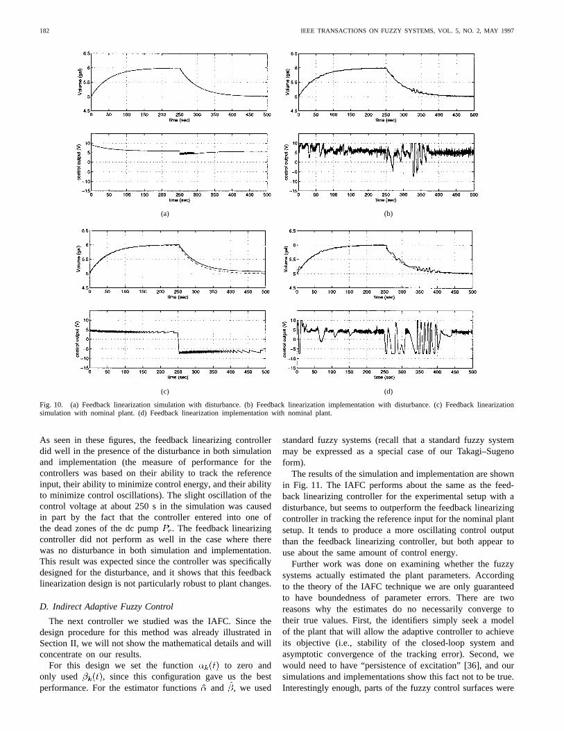
Fig. 10. (a) Feedback linearization simulation with disturbance. (b) Feedback linearization implementation with disturbance. (c) Feedback linearizationsimulation with nominal plant. (d) Feedback linearization implementation with nominal plant.

As seen in these figures, the feedback linearizing controllerdid well in the presence of the disturbance in both simulationand implementation (the measure of performance for thecontrollers was based on their ability to track the referenceinput, their ability to minimize control energy, and their abilityto minimize control oscillations). The slight oscillation of thecontrol voltage at about 250 s in the simulation was causedin part by the fact that the controller entered into one ofthe dead zones of the dc pump. The feedback linearizingcontroller did not perform as well in the case where therewas no disturbance in both simulation and implementation.This result was expected since the controller was specificallydesigned for the disturbance, and it shows that this feedbacklinearization design is not particularly robust to plant changes.

D. Indirect Adaptive Fuzzy Control

The next controller we studied was the IAFC. Since thedesign procedure for this method was already illustrated inSection II, we will not show the mathematical details and willconcentrate on our results.

For this design we set the function to zero andonly used , since this configuration gave us the bestperformance. For the estimator functionsand , we used

standard fuzzy systems (recall that a standard fuzzy systemmay be expressed as a special case of our Takagi–Sugenoform).

The results of the simulation and implementation are shownin Fig. 11. The IAFC performs about the same as the feed-back linearizing controller for the experimental setup with adisturbance, but seems to outperform the feedback linearizingcontroller in tracking the reference input for the nominal plantsetup. It tends to produce a more oscillating control outputthan the feedback linearizing controller, but both appear touse about the same amount of control energy.

Further work was done on examining whether the fuzzysystems actually estimated the plant parameters. Accordingto the theory of the IAFC technique we are only guaranteedto have boundedness of parameter errors. There are tworeasons why the estimates do no necessarily converge totheir true values. First, the identifiers simply seek a modelof the plant that will allow the adaptive controller to achieveits objective (i.e., stability of the closed-loop system andasymptotic convergence of the tracking error). Second, wewould need to have “persistence of excitation” [36], and oursimulations and implementations show this fact not to be true.Interestingly enough, parts of the fuzzy control surfaces were


(a) (b)

(c) (d)

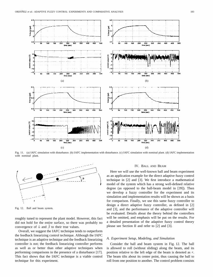
Fig. 11. (a) IAFC simulation with disturbance. (b) IAFC implementation with disturbance. (c) IAFC simulation with nominal plant. (d) IAFC implementationwith nominal plant.

Fig. 12. Ball and beam system.

roughly tuned to represent the plant model. However, this factdid not hold for the entire surface, so there was probably noconvergence of and to their true values.

Overall, we suggest the IAFC technique tends to outperformthe feedback linearizing control technique. Although the IAFCtechnique is an adaptive technique and the feedback linearizingcontroller is not; the feedback linearizing controller performsas well as or better than other adaptive techniques whenperforming comparisons in the presence of a disturbance [17].This fact shows that the IAFC technique is a viable controltechnique for this experiment.

IV. BALL AND BEAM

Here we will use the well-known ball and beam experimentas an application example for the direct adaptive fuzzy controltechnique in [2] and [3]. We first introduce a mathematicalmodel of the system which has a strong well-defined relativedegree (as opposed to the ball-beam model in [39]). Thenwe develop a fuzzy controller for the experiment and itssimulation and implementation results will be shown as a basisfor comparison. Finally, we use this same fuzzy controller todesign a direct adaptive fuzzy controller, as defined in [2]and [3], and the performance of the adaptive controller willbe evaluated. Details about the theory behind the controllerswill be omitted, and emphasis will be put on the results. Fora detailed presentation of the adaptive fuzzy control theoryplease see Section II and refer to [2] and [3].

A. Experiment Setup, Modeling, and Simulation

Consider the ball and beam system in Fig. 12. The ballis allowed to roll (without sliding) along the beam, and itsposition relative to the left edge of the beam is denoted as.The beam tilts about its center point, thus causing the ball toroll from one position to another. The control problem consists


Fig. 13. Motor-Ball-Beam Control Scheme:�r is the angle reference input,�e is the angle error, and� is the beam angle.

in designing a controller that tilts the beam in such a way thatthe ball is brought from its initial position to another desiredposition. The beam is driven by a dc motor whose shaft isattached to the center of the beam through a 50 : 1-turn ratiogear box. A ten-turn precision potentiometer is attached to themotor shaft to measure the angle of the beam. There are 32photodiodes mounted along the bottom of the beam, spacedat 0.75-in intervals along the slot over which the ball rolls.Two lamps are positioned above the experiment so that theyilluminate the whole beam area. The photodiodes detect theshadow cast by the ball to ascertain its position. Notice that thisposition sensing mechanism provides a discrete approximationto the actual position of the ball, and thus complicates thecontrol task. A resistive strip could have been used to providecontinuous position sensing, but this experiment was designedto be more challenging using the photodiodes (please see [40]for a detailed description of the setup).

Consider Fig. 13 for a block-diagram description of thesystem. Let be the input armature current to the motor,theangle of the beam, andthe position of the ball on the beam.A simple proportional-integral-derivative (PID) controller isused to drive the motor and to position the beam at any desiredangle. This controller takes as an input the errorbetweenan angle reference and the beam angle. The signal

is produced by the ball-position controller (which seeksto achieve our primary objective). By means of appropriatetuning of the PID controller, it is possible to achieve verygood angle tracking, and since the inner loop has much fasterdynamics than the outer loop, it can be considered virtuallyinvisible to the ball-position controller.

Let and . Then, a linear state-space modelof the motor is given by

, where , ,, and (the numerical values

come from the motor specifications and the beam dimensions).If we now let we can obtain two more equations whichrepresent the ball and beam dynamics when the beam angleis taken as the input, using Newton’s second law. Here, weare using the approximation (valid because thebeam angle varies within a small range around zero) to havethe input enter linearly. We have found that a reasonably goodmodel of our ball-beam system is given by

(26)

where and , and the system output

is . The numerical values take into account theacceleration due to gravity and the friction constant betweenthe ball and the beam (determined experimentally), and arescaled in such a way that the outputis in units of 0.75 in,which corresponds to the distance between the photodiodes.The function is an approximationto the acceleration due to friction that the ball experiences onthe beam.

If the output is repeatedly differentiated, we find that thesystem has a well-definedstrong relative degree[33], [34] offour. Furthermore, it is possible to determine that thezerodynamics [34] of the system are exponentially stable (thedetails of the calculations involved are very tedious and are,therefore, omitted).

For our simulations below, we use a fourth-orderRunge–Kutta numerical method with an integration stepsize of 0.001 s. In implementation, a sampling time of 0.01s is used.

B. A Fuzzy Controller for the Ball and Beam

We now describe our results for the ball and beam using astandard fuzzy system for ball position control (details on thecontroller are omitted for brevity). The fuzzy controller hastwo inputs: the position error (defined as , where

is the desired ball position) and the error derivative.We use singleton fuzzification for both inputs. Forwe takefive triangular membership functions; for we use three, andwe make a standard choice for the rule base. In the inferencemechanism we use minimum to represent the premise andproduct for the implication, and centroid defuzzification isapplied to obtain the output of the fuzzy system.

For all simulations and laboratory experiments, the ball wasinitially on position five on the beam (that is, it was set ontop of the photodiode number five, where the photodiodes arenumbered from 0 to 31 beginning at the left); the desiredposition is twelve during the first ten seconds, and then changesto eight for another 10 s. The discrete ball position sensingmechanism of the real system is also used in simulation—theball position controller receives not the exact value of, but itsposition index (as represented by the number of photodiodesalong the beam).

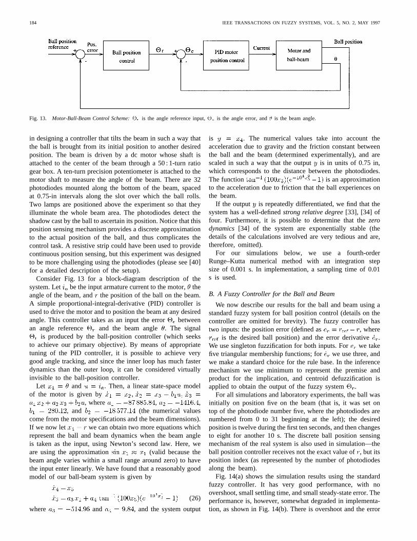
Fig. 14(a) shows the simulation results using the standardfuzzy controller. It has very good performance, with noovershoot, small settling time, and small steady-state error. Theperformance is, however, somewhat degraded in implementa-tion, as shown in Fig. 14(b). There is overshoot and the error


(a)

(b)

Fig. 14. Direct fuzzy controller. (a) Simulation results. (b) Implementationresults.

is larger. Notice the ball-position measurement noise [spikesbetween seventh and eighth seconds in Fig. 14(b)], which addsto the complexity of the control task.

C. Direct Adaptive Fuzzy Control

We will now use the fuzzy controller of the previous sectionto design a DAFC following the methodology of [2] and [3].It is expected that the adaptive controller will achieve animproved performance and have a greater robustness againstnoise. Two assumptions about the plant have to be verifiedto apply this technique. First, the system has to be minimumphase; this condition may be easily verified for our proposedmodel. As we mentioned above, the ball-beam model hasa relative degree of four. However, to simplify the designwe ignore the motor dynamics (notice that this assumptionrequires the motor control to be efficient enough, i.e., it shouldprovide good tracking with little lag; we can see that this is the

case in Fig. 14: the motor shaft anglefollows the referenceclosely), so we may use the approximation . In this

way, we only have to deal with the two-state system in (26).If we differentiate the output twice and take ,we find that

(27)

That is, the relative degree of the system that the ball positioncontroller “sees” is two, and it has no zero dynamics; therefore,it is minimum phase (note that the much more complicatedanalysis that does not discard the motor dynamics leads tonumerically similar results, with the system having a relativedegree of four and asymptotically stable zero dynamics).

The second plant assumption of [2] and [3] can also beverified from (27). Using the notation from these referenceslet . Then there exist constants and

such that . Take, for instance,and . It is also required that for some

, . The assumption holds if we let, since is a constant.

We will not show the development of the DAFC sinceit was already illustrated in Section II. However, there isone issue to notice: in our DAFC design we used the fuzzysystem described abovewithout any modificationsfor the term

(recall that a standard fuzzy system is a special case ofthe more general Takagi–Sugeno form we consider), and theadaptation laws adopted a simplified form.

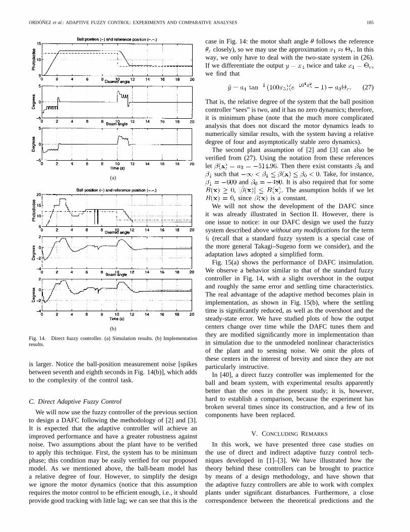
Fig. 15(a) shows the performance of DAFC insimulation.We observe a behavior similar to that of the standard fuzzycontroller in Fig. 14, with a slight overshoot in the outputand roughly the same error and settling time characteristics.The real advantage of the adaptive method becomes plain inimplementation, as shown in Fig. 15(b), where the settlingtime is significantly reduced, as well as the overshoot and thesteady-state error. We have studied plots of how the outputcenters change over time while the DAFC tunes them andthey are modified significantly more in implementation thanin simulation due to the unmodeled nonlinear characteristicsof the plant and to sensing noise. We omit the plots ofthese centers in the interest of brevity and since they are notparticularly instructive.

In [40], a direct fuzzy controller was implemented for theball and beam system, with experimental results apparentlybetter than the ones in the present study; it is, however,hard to establish a comparison, because the experiment hasbroken several times since its construction, and a few of itscomponents have been replaced.

V. CONCLUDING REMARKS

In this work, we have presented three case studies onthe use of direct and indirect adaptive fuzzy control tech-niques developed in [1]–[3]. We have illustrated how thetheory behind these controllers can be brought to practiceby means of a design methodology, and have shown thatthe adaptive fuzzy controllers are able to work with complexplants under significant disturbances. Furthermore, a closecorrespondence between the theoretical predictions and the


(a)

(b)

Fig. 15. Direct adaptive fuzzy controller. (a) Simulation results. (b) Imple-mentation results.

experimental results has been found. The performance of theadaptive fuzzy controllers has been compared with that ofseveral other techniques which, according to our experience,present a good behavior for the plants we used. In thecase of the rotational inverted pendulum, a comparison wasmade with a linear quadratic regulator and adaptive andnonadaptive feedback linearizing controllers. For the processcontrol problem, the comparison was made with nonadaptivefeedback linearization, and for the ball and beam we comparedwith a standard (nonadaptive) fuzzy controller.

Although the results we obtained seem to indicate that theDAFC and IAFC have comparable performance or are able tooutperform the techniques they were compared with, it is stillnecessary to evaluate the performance of the controllers undera greater variety of conditions. It remains to be investigatedhow robust the controllers are against many different typesof disturbances; for instance, we did not study how theadaptive fuzzy controllers react to “impact disturbances” on

the pendulum. Generally speaking, disturbances of this typepresent a great challenge for adaptive schemes, especiallyif there is a sloshing liquid at the endpoint. The invertedpendulum is an example of a system with marginally stablezero dynamics that because of its nature, provides insight intothe way the adaptive controllers work. And, as we saw, it waspossible to design a DAFC that gave us bounded states in spiteof the marginal stability of the zero dynamics. However, weprovided no theoretical justification of the fact that this designworked as it did. In the cases of the process control tank andthe ball-beam system, the adaptive fuzzy controllers were ableto compensate for some disturbances and sensing noise, but itstill seems possible that their performance could be improved(perhaps by further tuning of the techniques).

The results of our case studies suggest that investigating anextension of the adaptive schemes in [1]–[3] to certain types ofnonminimum phase systems might be fruitful; if accomplished,such an extension would broaden the application spectrumof adaptive techniques in general. In addition, the IAFC andDAFC are single-input single-output schemes, and an exten-sion to multi-input multi-output systems is currently underway; the indirect case has already been introduced in [41]. It isalso important to notice that the adaptive fuzzy controllers in[1]–[3] arecontinuous timetechniques; to implement them weused a digital computer, and thus were forced to implicitlyuse a discrete time approximation of the controllers. It isreasonable to think that a proof of stability is still applicablewhen a continuous time technique is discretized, but sucha study is outside the scope of the present work. Recently,(in [42]) the authors have introduced a stable discrete-timeadaptive control scheme for a class of nonlinear systems.

ACKNOWLEDGMENT

The authors would like to thank M. Widjaja, under thedirection of Prof. S. Yurkovich, for developing the rotationalinverted pendulum experiment. The process control experi-ment was initially set up by R. Garcar under the direction ofProf. U. Ozguner and the authors would like to thank themfor this. They would also like to thank P. Jaklitsch, who laterupdated the experiment and made several improvements to itunder the direction of Prof. S. Yurkovich, and J. Zumberge,working under the direction of Prof. K. Passino, who expandedon the improvements of P. Jacklitsch by coding all the softwarein C, improving the performance of the level measuringsensors, and adding an ac pump to establish the experimentaltestbed used for this study. They would also like to thank E.G. Laukonen, under the direction of Prof. S. Yurkovich, whodeveloped the ball and beam experiment.

REFERENCES

[1] J. T. Spooner and K. M. Passino, “Stable indirect adaptive control usingfuzzy systems and neural networks,” in34th IEEE Conf. Decision Contr.Proc., New Orleans, LA, Dec. 1995, pp. 243–248.

[2] , “Stable direct adaptive control using fuzzy systems and neuralnetworks,” in 34th IEEE Conf. Decision Contr. Proc.,New Orleans,LA, Dec. 1995, pp. 249–254.

[3] , “Stable adaptive control using fuzzy systems and neural net-works,” IEEE Trans. Fuzzy Syst.,vol. 4, pp. 339–359, Aug. 1996.


[4] L.-X. Wang, Adaptive Fuzzy Systems and Control: Design and StabiltyAnalysis. Englewood Cliffs, NJ: Prentice-Hall, 1994.

[5] K. M. Passino and S. Yurkovich, “Fuzzy control,” inHandbook onControl, W. Levine, Ed. Boca Raton, FL: CRC, 1996, pp. 1001–1017.

[6] D. Driankov, H. Hellendoorn, and M. M. Reinfrank,An Introduction toFuzzy Control. Heidelberg, Germany: Springer-Verlag, 1993.

[7] T. Procyk and E. Mamdani, “A linguistic self-organizing process con-troller,” Automatica,vol. 15, no. 1, pp. 15–30, 1979.

[8] J. R. Layne and K. M. Passino, “Fuzzy model reference learningcontrol,” J. Intell. Fuzzy Syst.,vol. 4, no. 1, pp. 33–47, 1996.

[9] , “Fuzzy model reference learning control,” inProc. 1st IEEEConf. Contr. Applicat.,Dayton, OH, Sept. 1992, pp. 686–691.

[10] , “Fuzzy model reference learning control for cargo ship steering,”IEEE Contr. Syst. Mag.,vol. 13, pp. 23–34, Dec. 1993.

[11] W. A. Kwong and K. M. Passino, “Dynamically focused fuzzy learningcontrol,” IEEE Trans. Syst., Man, Cybern.,vol. 26, pp. 53–74, Feb. 1996.

[12] J. Layne, K. Passino, and S. Yurkovich, “Fuzzy learning control for anti-skid braking systems,” inProc. IEEE Conf. Decision Contr.,Tucson,AZ, Dec. 1992, pp. 2523–2528.

[13] W. Kwong and K. Passino, “Fuzzy learning systems for aircraft controllaw reconfiguration,” inProc. IEEE Int. Symp. Intell. Contr.,Columbus,OH, Aug. 16–18, 1994, pp. 333–338.

[14] W. A. Kwong, K. M. Passino, E. G. Lauknonen, and S. Yurkovich,“Expert supervision of fuzzy learning systems for fault tolerant aircraftcontrol,” Proc. IEEE, Spec. Issue Fuzzy Logic Eng. Applicat.,vol. 83,pp. 466–483, Mar. 1995.

[15] , “Expert supervision of fuzzy learning systems with applicationsto reconfigurable control for aircraft,” inProc. IEEE Conf. DecisionContr., Orlando, FL, Dec. 1994, pp. 4116–4121.

[16] W. Lennon and K. Passino, “Intelligent control for brake systems,” inProc. IEEE Int. Symp. Intell. Contr.,Monterey, CA, Aug. 1995, pp.499–504.

[17] J. Zumberge and K. M. Passino, “A case study in intelligent control fora process control experiment,” inProc. IEEE Int. Symp. Intell. Contr.,Dearborn, MI, Sept. 1996, to be published.

[18] V. G. Moudgal, W. A. Kwong, K. M. Passino, and S. Yurkovich, “Fuzzylearning control for a flexible-link robot,”IEEE Trans. Fuzzy Syst.,vol.3, pp. 199–210, May 1995.

[19] T. A. Johansen, “Fuzzy model based control: Stability, robustness, andperformance issues,”IEEE Trans. Fuzzy Syst.,vol. 2, pp. 221–234, Aug.1994.

[20] C.-Y. Su and Y. Stepanenko, “Adaptive control of a class of nonlinearsystems with fuzzy logic,”IEEE Trans. Fuzzy Syst.,vol. 2, pp. 285–294,Nov. 1994.

[21] L.-X. Wang, “Stable adaptive fuzzy control of nonlinear systems,” inProc. 31st Conf. Decision Cont.,Tucson, AZ, 1992, pp. 2511–2516.

[22] , “A supervisory controller for fuzzy control systems that guar-antees stability,”IEEE Trans. Automat. Contr.,vol. 39, pp. 1845–1847,Sept. 1994.

[23] J. T. Spooner and K. M. Passino, “Stable adaptive fuzzy control foran automated highway system,” inProc. IEEE Int. Symp. Intell. Contr.,Monterey, CA, pp. 531–536, Aug. 1995.

[24] F.-C. Chen and H. K. Khalil, “Adaptive control of nonlinear systemsusing neural networks—A dead-zone approach,” inProc. Amer. Cont.Conf., Boston, MA, 1991, pp. 667–672.

[25] , “Adaptive control of nonlinear systems using neural networks,”Int. J. Contr.,vol. 55, pp. 1299–1317, 1992.

[26] F.-C. Chen and W.-C. Tsao, “Adaptive control of linearizable discrete-time systems,” inProc. Amer. Contr. Conf.,Baltimore, MD, June 1994,pp. 880–881.

[27] F.-C. Chen and H. K. Khalil, “Adaptive control of a class of nonlineardiscrete-time systems using neural networks,”IEEE Trans. Automat.Contr., vol. 40, pp. 791–801, May 1995.

[28] M. M. Polycarpou and P. A. Ioannou, “Identification and control ofnonlinear systems using neural network models: Design and stabilityanalysis,” Univ. Southern California, Dept. Electrical Engineering, Syst.Rep. 91-09-01, Sept. 1991.

[29] G. A. Rovithakis and M. A. Christodoulou, “Adaptive control ofunknown plants using dynamical neural networks,”IEEE Trans. Syst.,Man., Cybern.,vol. 24, pp. 400–412, Mar. 1994.

[30] R. Ordonez, J. T. Spooner, and K. M. Passino, “Experiments andcomparative analyses in adaptive fuzzy control,” inProc. IEEE Int.Symp. Intell. Contr.,Dearborn, MI, Sept. 1996, to be published.

[31] M. Widjaja and S. Yurkovich, “Intelligent control for swing up andbalancing of an inverted pendulum system,” inProc. 4th IEEE Int. Conf.Contr. Applicat.,Albany, NY, Sept. 1995, pp. 534–542.

[32] S. Yurkovich and M. Widjaja, “Fuzzy controller synthesis for an invertedpendulum system,”IFAC Contr. Eng. Practice,vol. 4, pp. 445–469, Apr.1996.

[33] J.-J. E. Slotine and W. Li,Applied Nonlinear Control. EnglewoodCliffs, NJ: Prentice-Hall, 1991.

[34] M. Vidyasagar,Nonlinear System Analysis,2nd ed. Englewood Cliffs,NJ: Prentice-Hall, 1993.

[35] S. S. Sastry and A. Isidori, “Adaptive control of linearizable systems,”IEEE Trans. Automat. Contr.,vol. 34, pp. 1123–1131, Nov. 1989.

[36] S. S. Sastry and M. Bodson,Adaptive Control: Stability, Convergence,and Robustness.Englewood Cliffs, NJ: Prentice-Hall, 1989.

[37] T. Takagi and M. Sugeno, “Fuzzy identification of systems and itsapplication to modeling and control,”IEEE Trans. Syst., Man, Cybern.,vol. 15, pp. 116–132, 1985.

[38] H. Thomas and E. Sebastian, “Approximately time optimal fuzzy controlof a two-tank system,”IEEE Contr. Syst. Mag.,vol. 14, pp. 24–30, June1994.

[39] S. S. John Hauser and P. Kokotovic, “Nonlinear control via approximateinput-output linearization: The ball and beam example,”IEEE Trans.Automat. Contr.,vol. 37, pp. 392–398, Mar. 1992.

[40] E. G. Laukonen and S. Yurkovich, “A ball and beam testbed for fuzzyidentification and control design,” inAmer. Contr. Conf.,San Francisco,CA, June 1993, vol. 1, pp. 665–669.

[41] R. E. Ordonez, J. T. Spooner, and K. M. Passino, “Stable multi-inputmulti-output adaptive fuzzy control,” inIEEE Conf. Decision Contr.,Dearborn, MI, Sept. 1996, pp. 31–36.

[42] J. T. Spooner, R. Ordonez, and K. M. Passino, “Stable direct adaptivecontrol of a class of discrete time nonlinear systems,” inIFAC WorldCongress,San Francisco, CA, July 1996, vol. K, pp. 343–348, invitedpaper.

Raul Ord o~nez was born in Guayaquil, Ecuador,on February 18, 1971. He received the B.S. degree(summa cum laude) from the Instituto Tecnologicoy de Estudios Superiores de Monterrey, Monterrey,Mexico, in 1994, and the M.S. degree from TheOhio State University, Columbus, OH, in 1996, bothin electrical engineering. He is currently workingtoward the Ph.D. at The Ohio State University.

In 1994, he received a Litton Fellowship andhas since worked as a Teaching and a ResearchAssistant. His research interests include fuzzy and

neural control, adaptive control, and stability analysis for nonlinear systems.

Jon Zumberge was born in Dayton, OH, in 1971.He received the B.S.E.E. degree, in 1994, and theM.S.E.E. degree, in 1996, both from The Ohio StateUniversity, Columbus.

He is currently working for Delphi Chassis Sys-tems, Dayton as a Project Engineer. His researchinterests include adaptive fuzzy control, supervisoryfuzzy control, and nonlinear identification via fuzzysystems.

Jeffrey T. Spooner received the B.A. degree inphysics from Wittenberg University, Springfield,OH, in 1991, the B.S. degree in electrical engineer-ing from The Ohio State University, Columbus, in1993, and the M.S. degree in electrical engineering(with a specialization in control systems), in 1995,from The Ohio State University, Columbus.

Since 1995, he has been with the Control Subsys-tems Department at Sandia National Laboratories,Albuquerque, NM. His areas of interest includeadaptive control, fuzzy systems, neural networks,and modeling.


Kevin M. Passino (S’79–M’90–SM’96) receivedthe B.S.E.E. degree from Tri-State University, An-gola, IN, in 1983, and the M.S. and Ph.D. degrees inelectrical engineering from the University of NotreDame, IN, in 1989.

He has worked in the control systems group atMagnavox Electronic Systems Co., Ft. Wayne, IN,on research in missile control, and at McDonnellAircraft Co., St. Louis, MI, on research in flightcontrol. He spent a year at Notre Dame as a VisitingAssistant Professor, and is currently an Associate

Professor in the Department of Electrical Engineering at The Ohio StateUniversity, Columbus. He is an Associate Editor for the IEEE TRANSACTIONS

ON AUTOMATIC CONTROL, served as the Guest Editor for the 1993IEEE ControlSystems Magazine Special Issue on Intelligent Controland Guest Editor fora special track of papers on intelligent control forIEEE Expert Magazinein 1996, and is on the Editorial Board of theInternational Journal forEngineering Applications of Artificial Intelligence. He is co-editor (with P. J.Antsaklis) of the bookAn Introduction to Intelligent and Autonomous Control(Norwell, MA: Kluwer, 1993). His research interests include intelligentand autonomous control techniques, nonlinear analysis of intelligent controlsystems, failure detection and identification systems, and genetic algorithmsfor control.

Dr. Passino is a member of the IEEE Control Systems Society Board ofGovernors. He was the Publicity co-chair for the IEEE Conference on Decisionand Control in Japan in 1996 and is the Workshops Chair for the 1997 IEEEConference on Decision and Control. He was a Program Chairman for the8th IEEE International Symposium on Intelligent Control in 1993, served asthe Finance Chair for the 9th IEEE International Symposium on IntelligentControl, and is serving as the General Chair for the 11th IEEE InternationalSymposium on Intelligent Control.

adaptive fuzzy control experiments and comparative analyses

Documents