adaptive high-order methods for elliptic problems: … · adaptive high-order methods for elliptic...
TRANSCRIPT

Adaptive High-Order Methods for Elliptic Problems:
Convergence and Optimality
Claudio Canuto
Department of Mathematical SciencesPolitecnico di Torino, Italy
Joint work with
Ricardo H. Nochetto, University of Maryland, U.S.A.
Rob Stevenson, Korteweg-de Vries Institute for Mathematics, The Netherlands
Marco Verani, Politecnico di Milano, Italy
Foundations of Computational MathematicsBarcelona, July 14 2017

Outline
Introduction
Adaptive Fourier methods
A framework for hp-Adaptivity
hp-Adaptive Approximation
Basic hp-Adaptive Algorithm
Realizations of the Algorithm
Conclusions

Introduction Adaptive Fourier methods hp-framework hp-Adaptive Approximation Basic hp-AFEM Realizations Conclusions
Outline
Introduction
Adaptive Fourier methods
A framework for hp-Adaptivity
hp-Adaptive Approximation
Basic hp-Adaptive Algorithm
Realizations of the Algorithm
Conclusions
hp-AFEM Claudio Canuto

Introduction Adaptive Fourier methods hp-framework hp-Adaptive Approximation Basic hp-AFEM Realizations Conclusions
Adaptive approximation of elliptic problems: the state of the art
• Adaptivity for finite-order methods [wavelets, h-type finite elements]:well-understood in terms of algorithms and theory (convergence, optimality)
[Dorfler 1996, Morin, Nochetto and Siebert 2000, Binev, Dahmen and DeVore 2004,
Stevenson 2007, Cascon, Kreuzer, Nochetto and Siebert 2008 ]
• Adaptivity for high-order methods [spectral, hp-type finite elements]:heuristic algorithms, partial theory
I A posteriori error analysis:
[Gui and Babuska 1986, Oden, Demkowicz et al ’89, Bernardi ’96, Ainsworthand Senior ’98, Schmidt and Siebert ’00, Melenk and Wohlmuth ’01, Heuvelinand Rannacher ’03, Houston and Suli ’05, Eibner and Melenk ’07, Braess,Pillwein and Schoberl ’08, Ern and Vohralık ’14, ... ]
I Convergence and optimality:
[Scherer 1982, Schmidt and Siebert 2000, Dorfler and Heuveline 2007, Burgand Dorfler 2011, Bank, Parsania, and Sauter 2014, our work (2012 →)]
hp-AFEM Claudio Canuto
Introduction Adaptive Fourier methods hp-framework hp-Adaptive Approximation Basic hp-AFEM Realizations Conclusions
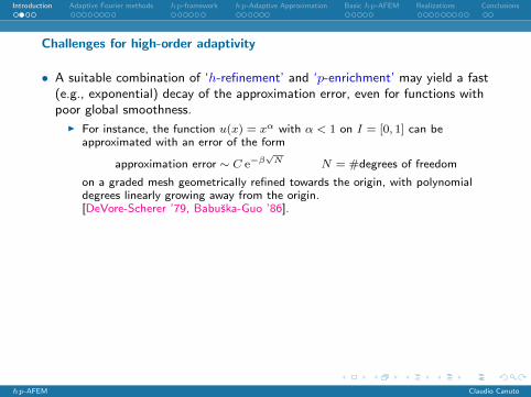
Challenges for high-order adaptivity
• A suitable combination of ‘h-refinement’ and ‘p-enrichment’ may yield a fast(e.g., exponential) decay of the approximation error, even for functions withpoor global smoothness.
I For instance, the function u(x) = xα with α < 1 on I = [0, 1] can beapproximated with an error of the form
approximation error ∼ C e−β√N N = #degrees of freedom
on a graded mesh geometrically refined towards the origin, with polynomialdegrees linearly growing away from the origin.[DeVore-Scherer ’79, Babuska-Guo ’86].
• Need of dealing with approximation classes of functions for which the (best)approximation error decays faster than algebraically (e.g., exponentially).
• The choice between ‘h-refinement’ and ‘p-enrichment’ is quite delicate.
In an iterative adaptive algorithm, one of the two choices may appearpreferable in an earlier stage, but eventually it may reveal itself short-sightedand non-optimal.
One should incorporate the possibility of stepping back, and correcting earlyerrors in the adaptive strategy.
hp-AFEM Claudio Canuto

Introduction Adaptive Fourier methods hp-framework hp-Adaptive Approximation Basic hp-AFEM Realizations Conclusions
Approximation classes
• Best N-term approximation error: Given v ∈ V , define
σN (v) = infVN⊂V
dimVN=N
infw∈VN
‖v − w‖V .
• Decay vs N identifies an approximation class:
σN (v) . φ(N) with φ→ 0 as N →∞.
• Algebraic class (finite-order methods):
v ∈ AsB iff |v|AsB
:= supN
σN (v)Ns/d <∞.
• Exponential class (infinite-order methods):
v ∈ Aη,tG iff |v|Aη,tG
:= supN
σN (v)eηNτ
<∞.
hp-AFEM Claudio Canuto

Introduction Adaptive Fourier methods hp-framework hp-Adaptive Approximation Basic hp-AFEM Realizations Conclusions
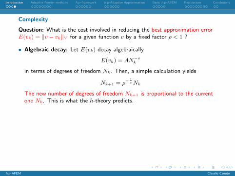
Complexity
Question: What is the cost involved in reducing the best approximation errorE(vk) = ‖v − vk‖V for a given function v by a fixed factor ρ < 1 ?
• Algebraic decay: Let E(vk) decay algebraically
E(vk) = AN−sk
in terms of degrees of freedom Nk. Then, a simple calculation yields
Nk+1 = ρ−1sNk
The new number of degrees of freedom Nk+1 is proportional to the currentone Nk. This is what the h-theory predicts.
• Exponential decay: Let E(vk) decay exponentially
E(vk) = Ae−ηNk .
Then, a simple calculation reveals that
Nk+1 −Nk = −η−1 log ρ
and the number of degrees of freedom must only grow by an additiveconstant. This property is very delicate to prove!
hp-AFEM Claudio Canuto
Introduction Adaptive Fourier methods hp-framework hp-Adaptive Approximation Basic hp-AFEM Realizations Conclusions
Complexity
Question: What is the cost involved in reducing the best approximation errorE(vk) = ‖v − vk‖V for a given function v by a fixed factor ρ < 1 ?
• Algebraic decay: Let E(vk) decay algebraically
E(vk) = AN−sk
in terms of degrees of freedom Nk. Then, a simple calculation yields
Nk+1 = ρ−1sNk
The new number of degrees of freedom Nk+1 is proportional to the currentone Nk. This is what the h-theory predicts.
• Exponential decay: Let E(vk) decay exponentially
E(vk) = Ae−ηNk .
Then, a simple calculation reveals that
Nk+1 −Nk = −η−1 log ρ
and the number of degrees of freedom must only grow by an additiveconstant. This property is very delicate to prove!
hp-AFEM Claudio Canuto

Introduction Adaptive Fourier methods hp-framework hp-Adaptive Approximation Basic hp-AFEM Realizations Conclusions
Outline
Introduction
Adaptive Fourier methods
A framework for hp-Adaptivity
hp-Adaptive Approximation
Basic hp-Adaptive Algorithm
Realizations of the Algorithm
Conclusions
hp-AFEM Claudio Canuto
Introduction Adaptive Fourier methods hp-framework hp-Adaptive Approximation Basic hp-AFEM Realizations Conclusions
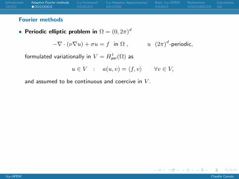
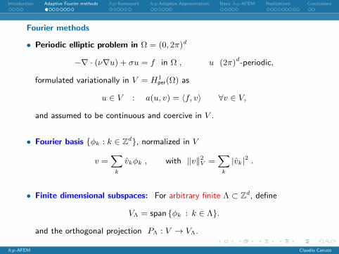
Fourier methods
• Periodic elliptic problem in Ω = (0, 2π)d
−∇ · (ν∇u) + σu = f in Ω , u (2π)d-periodic,
formulated variationally in V = H1per(Ω) as
u ∈ V : a(u, v) = 〈f, v〉 ∀v ∈ V,
and assumed to be continuous and coercive in V .
• Fourier basis φk : k ∈ Zd, normalized in V
v =∑k
vkφk , with ‖v‖2V =∑k
|vk|2 .
• Finite dimensional subspaces: For arbitrary finite Λ ⊂ Zd, define
VΛ = span φk : k ∈ Λ.
and the orthogonal projection PΛ : V → VΛ.
hp-AFEM Claudio Canuto

Introduction Adaptive Fourier methods hp-framework hp-Adaptive Approximation Basic hp-AFEM Realizations Conclusions
Fourier methods
• Periodic elliptic problem in Ω = (0, 2π)d
−∇ · (ν∇u) + σu = f in Ω , u (2π)d-periodic,
formulated variationally in V = H1per(Ω) as
u ∈ V : a(u, v) = 〈f, v〉 ∀v ∈ V,
and assumed to be continuous and coercive in V .
• Fourier basis φk : k ∈ Zd, normalized in V
v =∑k
vkφk , with ‖v‖2V =∑k
|vk|2 .
• Finite dimensional subspaces: For arbitrary finite Λ ⊂ Zd, define
VΛ = span φk : k ∈ Λ.
and the orthogonal projection PΛ : V → VΛ.
hp-AFEM Claudio Canuto

Introduction Adaptive Fourier methods hp-framework hp-Adaptive Approximation Basic hp-AFEM Realizations Conclusions
Galerkin approximation and residual
• Galerkin projection
uΛ ∈ VΛ : a(uΛ, vΛ) = 〈f, vΛ〉 ∀vΛ ∈ VΛ .
• Residual rΛ = r(uΛ) ∈ V ′ defined by
〈rΛ, v〉 = 〈f, vΛ〉 − a(uΛ, v) ∀v ∈ V.
It satisfies‖rΛ‖2V ′ =
∑k 6∈Λ
|rk|2, rk = 〈rΛ, φk〉.
• (Ideal) efficient and reliable error estimator
1
α∗‖r(uΛ)‖V ′ ≤ ‖u− uΛ‖V ≤
1
α∗‖r(uΛ)‖V ′ ,
hp-AFEM Claudio Canuto
Introduction Adaptive Fourier methods hp-framework hp-Adaptive Approximation Basic hp-AFEM Realizations Conclusions
Dorfler marking
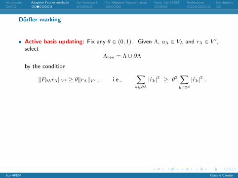
• Active basis updating: Fix any θ ∈ (0, 1). Given Λ, uΛ ∈ VΛ and rΛ ∈ V ′,select
Λnew = Λ ∪ ∂Λ
by the condition
‖P∂ΛrΛ‖V ′ ≥ θ‖rΛ‖V ′ , i.e.,∑k∈∂Λ
|rk|2 ≥ θ2∑k∈Zd
|rk|2 .
• Minimality: ∂Λ may be chosen of minimal cardinality by a greedy approach,bases on the decreasing rearrangement of the moduli of the Fouriercoefficients of rΛ.
• Feasibility: Exploiting some more information on data, a feasible versionexists, which requires exploring only a finite number of Fourier coefficients ofrΛ.
hp-AFEM Claudio Canuto

Introduction Adaptive Fourier methods hp-framework hp-Adaptive Approximation Basic hp-AFEM Realizations Conclusions
Dorfler marking
• Active basis updating: Fix any θ ∈ (0, 1). Given Λ, uΛ ∈ VΛ and rΛ ∈ V ′,select
Λnew = Λ ∪ ∂Λ
by the condition
‖P∂ΛrΛ‖V ′ ≥ θ‖rΛ‖V ′ , i.e.,∑k∈∂Λ
|rk|2 ≥ θ2∑k∈Zd
|rk|2 .
• Minimality: ∂Λ may be chosen of minimal cardinality by a greedy approach,bases on the decreasing rearrangement of the moduli of the Fouriercoefficients of rΛ.
• Feasibility: Exploiting some more information on data, a feasible versionexists, which requires exploring only a finite number of Fourier coefficients ofrΛ.
hp-AFEM Claudio Canuto
Introduction Adaptive Fourier methods hp-framework hp-Adaptive Approximation Basic hp-AFEM Realizations Conclusions
An ideal adaptive algorithm
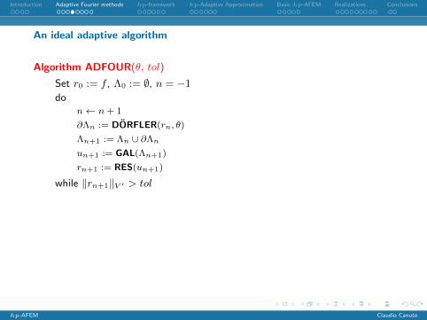
Algorithm ADFOUR(θ, tol)
Set r0 := f , Λ0 := ∅, n = −1
don← n+ 1
∂Λn := DORFLER(rn, θ)
Λn+1 := Λn ∪ ∂Λn
un+1 := GAL(Λn+1)
rn+1 := RES(un+1)
while ‖rn+1‖V ′ > tol
Theorem (contraction property of ADFOUR). Let θ ∈ (0, 1) and letΛn, unn≥0 be the sequence generated by the adaptive algorithm above.Then,
|||u− un+1||| ≤√
1− α∗α∗θ2︸ ︷︷ ︸
ρ(θ)<1
|||u− un|||
where |||v||| =√a(v, v).
hp-AFEM Claudio Canuto

Introduction Adaptive Fourier methods hp-framework hp-Adaptive Approximation Basic hp-AFEM Realizations Conclusions
An ideal adaptive algorithm
Algorithm ADFOUR(θ, tol)
Set r0 := f , Λ0 := ∅, n = −1
don← n+ 1
∂Λn := DORFLER(rn, θ)
Λn+1 := Λn ∪ ∂Λn
un+1 := GAL(Λn+1)
rn+1 := RES(un+1)
while ‖rn+1‖V ′ > tol
Theorem (contraction property of ADFOUR). Let θ ∈ (0, 1) and letΛn, unn≥0 be the sequence generated by the adaptive algorithm above.Then,
|||u− un+1||| ≤√
1− α∗α∗θ2︸ ︷︷ ︸
ρ(θ)<1
|||u− un|||
where |||v||| =√a(v, v).
hp-AFEM Claudio Canuto

Introduction Adaptive Fourier methods hp-framework hp-Adaptive Approximation Basic hp-AFEM Realizations Conclusions
A more aggressive version
If the coefficients of the equation are analytic, the Galerkin matrix is “quasisparse”. Exploiting this property, one can slightly enrich the active setproduced by Dorfler’s marking, and push the contraction constant towards 0 .
Algorithm A-ADFOUR(θ, tol)
Set r0 := f , Λ0 := ∅, n = −1do
n← n+ 1
∂Λn := DORFLER(rn, θ)
∂Λn := ENRICH(∂Λn, θ)
Λn+1 := Λn ∪ ∂Λnun+1 := GAL(Λn+1)
rn+1 := RES(un+1)
while ‖rn+1‖V ′ > tol
Theorem (contraction property of A-ADFOUR). Let θ ∈ (0, 1) and letΛn, unn≥0 be the sequence generated by A-ADFOUR. Then,
|||u− un+1||| ≤ 2
√α∗α∗
√1− θ2 |||u− un||| .
hp-AFEM Claudio Canuto

Introduction Adaptive Fourier methods hp-framework hp-Adaptive Approximation Basic hp-AFEM Realizations Conclusions
Optimality issues
• Target cardinality growth: If the solution u belongs to some exponentialclass Aη,tG , one should expect
#Λn ≤
(1
ηlog
|u|Aη,tG
‖u− un‖
)1/τ
+ C , n = 0, 1, 2, . . .
• Residual obstruction: Dorfler marking is based on the current residual rΛ.In general, this belongs to a worse approximation class than the solution.
v ∈ Aη,tG ⇒ r(v) ∈ Aη,tG for some η ≤ η, τ ≤ τ.
• Estimate on cardinality growth:
#Λn ≤
(1
ηlog
|u|Aη,tG
‖u− un‖
)1/τ
+ C , n = 0, 1, 2, . . .
• Remedies...
hp-AFEM Claudio Canuto

Introduction Adaptive Fourier methods hp-framework hp-Adaptive Approximation Basic hp-AFEM Realizations Conclusions
Remedy I: incorporating a coarsening step
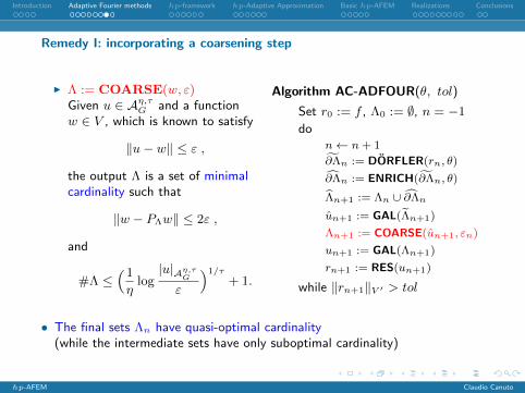
I Λ := COARSE(w, ε)Given u ∈ Aη,τG and a functionw ∈ V , which is known to satisfy
‖u− w‖ ≤ ε ,
the output Λ is a set of minimalcardinality such that
‖w − PΛw‖ ≤ 2ε ,
and
#Λ ≤(1
ηlog|u|Aη,τ
G
ε
)1/τ
+ 1.
Algorithm AC-ADFOUR(θ, tol)
Set r0 := f , Λ0 := ∅, n = −1
don← n+ 1
∂Λn := DORFLER(rn, θ)
∂Λn := ENRICH(∂Λn, θ)
Λn+1 := Λn ∪ ∂Λn
un+1 := GAL(Λn+1)
Λn+1 := COARSE(un+1, εn)
un+1 := GAL(Λn+1)
rn+1 := RES(un+1)
while ‖rn+1‖V ′ > tol
• The final sets Λn have quasi-optimal cardinality(while the intermediate sets have only suboptimal cardinality)
hp-AFEM Claudio Canuto
Introduction Adaptive Fourier methods hp-framework hp-Adaptive Approximation Basic hp-AFEM Realizations Conclusions
Remedy I: incorporating a coarsening step
I Λ := COARSE(w, ε)Given u ∈ Aη,τG and a functionw ∈ V , which is known to satisfy
‖u− w‖ ≤ ε ,
the output Λ is a set of minimalcardinality such that
‖w − PΛw‖ ≤ 2ε ,
and
#Λ ≤(1
ηlog|u|Aη,τ
G
ε
)1/τ
+ 1.
Algorithm AC-ADFOUR(θ, tol)
Set r0 := f , Λ0 := ∅, n = −1
don← n+ 1
∂Λn := DORFLER(rn, θ)
∂Λn := ENRICH(∂Λn, θ)
Λn+1 := Λn ∪ ∂Λn
un+1 := GAL(Λn+1)
Λn+1 := COARSE(un+1, εn)
un+1 := GAL(Λn+1)
rn+1 := RES(un+1)
while ‖rn+1‖V ′ > tol
• The final sets Λn have quasi-optimal cardinality(while the intermediate sets have only suboptimal cardinality)
hp-AFEM Claudio Canuto

Introduction Adaptive Fourier methods hp-framework hp-Adaptive Approximation Basic hp-AFEM Realizations Conclusions
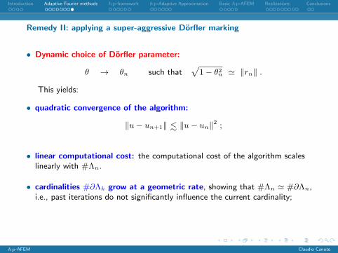
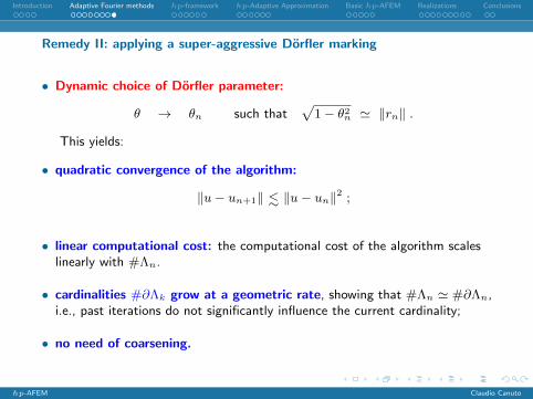
Remedy II: applying a super-aggressive Dorfler marking
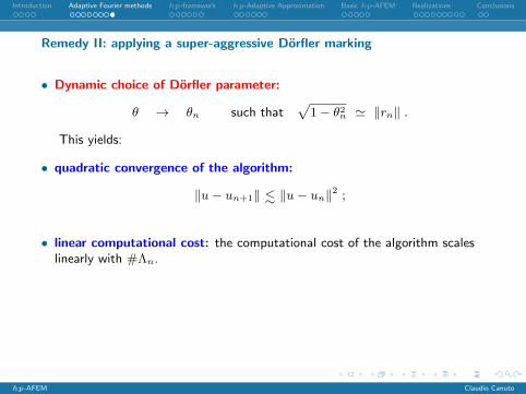
• Dynamic choice of Dorfler parameter:
θ → θn such that√
1− θ2n ' ‖rn‖ .
This yields:
• quadratic convergence of the algorithm:
‖u− un+1‖ <∼ ‖u− un‖2 ;
• linear computational cost: the computational cost of the algorithm scaleslinearly with #Λn.
• cardinalities #∂Λk grow at a geometric rate, showing that #Λn ' #∂Λn,i.e., past iterations do not significantly influence the current cardinality;
• no need of coarsening.
hp-AFEM Claudio Canuto

Introduction Adaptive Fourier methods hp-framework hp-Adaptive Approximation Basic hp-AFEM Realizations Conclusions
Remedy II: applying a super-aggressive Dorfler marking
• Dynamic choice of Dorfler parameter:
θ → θn such that√
1− θ2n ' ‖rn‖ .
This yields:
• quadratic convergence of the algorithm:
‖u− un+1‖ <∼ ‖u− un‖2 ;
• linear computational cost: the computational cost of the algorithm scaleslinearly with #Λn.
• cardinalities #∂Λk grow at a geometric rate, showing that #Λn ' #∂Λn,i.e., past iterations do not significantly influence the current cardinality;
• no need of coarsening.
hp-AFEM Claudio Canuto

Introduction Adaptive Fourier methods hp-framework hp-Adaptive Approximation Basic hp-AFEM Realizations Conclusions
Outline
Introduction
Adaptive Fourier methods
A framework for hp-Adaptivity
hp-Adaptive Approximation
Basic hp-Adaptive Algorithm
Realizations of the Algorithm
Conclusions
hp-AFEM Claudio Canuto

Introduction Adaptive Fourier methods hp-framework hp-Adaptive Approximation Basic hp-AFEM Realizations Conclusions
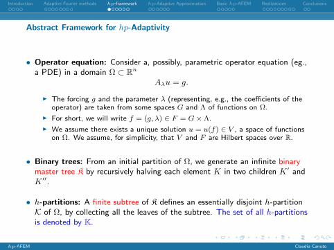
Abstract Framework for hp-Adaptivity
• Operator equation: Consider a, possibly, parametric operator equation (eg.,a PDE) in a domain Ω ⊂ Rn
Aλu = g.
I The forcing g and the parameter λ (representing, e.g., the coefficients of theoperator) are taken from some spaces G and Λ of functions on Ω.
I For short, we will write f = (g, λ) ∈ F = G× Λ.
I We assume there exists a unique solution u = u(f) ∈ V , a space of functionson Ω. We assume, for simplicity, that V and F are Hilbert spaces over R.
• Binary trees: From an initial partition of Ω, we generate an infinite binarymaster tree K by recursively halving each element K in two children K′ andK′′.
• h-partitions: A finite subtree of K defines an essentially disjoint h-partitionK of Ω, by collecting all the leaves of the subtree. The set of all h-partitionsis denoted by K.
hp-AFEM Claudio Canuto
Introduction Adaptive Fourier methods hp-framework hp-Adaptive Approximation Basic hp-AFEM Realizations Conclusions
Abstract Framework for hp-Adaptivity
• Operator equation: Consider a, possibly, parametric operator equation (eg.,a PDE) in a domain Ω ⊂ Rn
Aλu = g.
I The forcing g and the parameter λ (representing, e.g., the coefficients of theoperator) are taken from some spaces G and Λ of functions on Ω.
I For short, we will write f = (g, λ) ∈ F = G× Λ.
I We assume there exists a unique solution u = u(f) ∈ V , a space of functionson Ω. We assume, for simplicity, that V and F are Hilbert spaces over R.
• Binary trees: From an initial partition of Ω, we generate an infinite binarymaster tree K by recursively halving each element K in two children K′ andK′′.
• h-partitions: A finite subtree of K defines an essentially disjoint h-partitionK of Ω, by collecting all the leaves of the subtree. The set of all h-partitionsis denoted by K.
hp-AFEM Claudio Canuto

Introduction Adaptive Fourier methods hp-framework hp-Adaptive Approximation Basic hp-AFEM Realizations Conclusions
• hp-partitions: A hp-element is a pair D = (K, d) ∈ K× N, i.e., a geometricelement K together with a dimension d.
Given a h-partition K, an associated hp-partition of Ω is a collection
D = D = (KD, dD) : KD ∈ K.
The set of all hp-partitions is denoted by D.
hp-AFEM Claudio Canuto

Introduction Adaptive Fourier methods hp-framework hp-Adaptive Approximation Basic hp-AFEM Realizations Conclusions
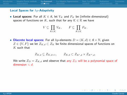
Local Spaces for hp-Adaptivity
• Local spaces: For all K ∈ K, let VK and FK be (infinite dimensional)spaces of functions on K, such that for any K ∈ K we have
V ⊆∏K∈K
VK , F ⊆∏K∈K
FK .
• Discrete local spaces: For all hp-elements D = (K, d) ∈ K× N, givenZ ∈ V, F we let ZK,d ⊂ ZK be finite dimensional spaces of functions onK such that
ZK,d ⊆ ZK,d+1, ZK,d ⊂ ZK′,d × ZK′′,d.
We write ZD = ZK,d and observe that any ZD will be a polynomial space ofdimension h d.
• Example: When K is an n-simplex, VK,d may be chosen as Pp(K), wherethe associated polynomial degree p = p(d) can be defined as the largestvalue in N such that dimPp−1(K) =
(n+p−1p−1
)≤ d.
I This definition normalizes the starting value p(1) = 1 for all n ∈ N.I Only for n = 1, it holds that p(d) = d for all d ∈ N.
hp-AFEM Claudio Canuto
Introduction Adaptive Fourier methods hp-framework hp-Adaptive Approximation Basic hp-AFEM Realizations Conclusions
Local Spaces for hp-Adaptivity
• Local spaces: For all K ∈ K, let VK and FK be (infinite dimensional)spaces of functions on K, such that for any K ∈ K we have
V ⊆∏K∈K
VK , F ⊆∏K∈K
FK .
• Discrete local spaces: For all hp-elements D = (K, d) ∈ K× N, givenZ ∈ V, F we let ZK,d ⊂ ZK be finite dimensional spaces of functions onK such that
ZK,d ⊆ ZK,d+1, ZK,d ⊂ ZK′,d × ZK′′,d.
We write ZD = ZK,d and observe that any ZD will be a polynomial space ofdimension h d.
• Example: When K is an n-simplex, VK,d may be chosen as Pp(K), wherethe associated polynomial degree p = p(d) can be defined as the largestvalue in N such that dimPp−1(K) =
(n+p−1p−1
)≤ d.
I This definition normalizes the starting value p(1) = 1 for all n ∈ N.I Only for n = 1, it holds that p(d) = d for all d ∈ N.
hp-AFEM Claudio Canuto

Introduction Adaptive Fourier methods hp-framework hp-Adaptive Approximation Basic hp-AFEM Realizations Conclusions
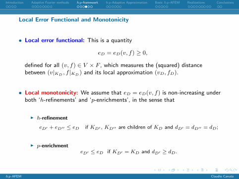
Local Error Functional and Monotonicity
• Local error functional: This is a quantity
eD = eD(v, f) ≥ 0,
defined for all (v, f) ∈ V × F , which measures the (squared) distancebetween (v|KD , f |KD ) and its local approximation (vD, fD).
• Local monotonicity: We assume that eD = eD(v, f) is non-increasing underboth ‘h-refinements’ and ‘p-enrichments’, in the sense that
I h-refinement
eD′ + eD′′ ≤ eD if KD′ , KD′′ are children of KD and dD′ = dD′′ = dD;
I p-enrichmenteD′ ≤ eD if KD′ = KD and dD′ ≥ dD.
hp-AFEM Claudio Canuto
Introduction Adaptive Fourier methods hp-framework hp-Adaptive Approximation Basic hp-AFEM Realizations Conclusions
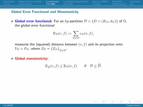
Global Error Functional and Monotonicity
• Global error functional: For an hp-partition D = D = (KD, dD) of Ω,the global error functional
ED(v, f) :=∑D∈D
eD(v, f),
measures the (squared) distance between (v, f) and its projection ontoVD × FD, where ZD =
(ZD)D∈D.
• Global monotonicity:
ED(v, f) ≤ ED(v, f) if D ≤ D.
• Notation:
I The cardinality of D is defined as #D :=∑D∈D dD (dD local dimension).
I The set D of all hp-partitions contains the subset Dc of the ‘conforming’partitions. We assume that for any D ∈ D there exists a conforming partitionC(D) such that
D ≤ C(D).
hp-AFEM Claudio Canuto

Introduction Adaptive Fourier methods hp-framework hp-Adaptive Approximation Basic hp-AFEM Realizations Conclusions
Example of Choice of Error Functional eD
• Consider the model elliptic problem in Ω
−∆u = f, u = 0 in ∂Ω,
• Define as a local error functional
eD(v, f) := |v − P 1pDv|
2H1(KD) +
1
κ‖p−1D hD(f − P 0
pD−1f)‖2L2(KD) ∀D ∈ D,
whereI P 1
p , P 0p resp. are orthogonal projectors on Pp(KD) in the inner products of
L2(KD), H10 (KD), resp.
I κ is a parameter to be chosen later on.
hp-AFEM Claudio Canuto

Introduction Adaptive Fourier methods hp-framework hp-Adaptive Approximation Basic hp-AFEM Realizations Conclusions
Outline
Introduction
Adaptive Fourier methods
A framework for hp-Adaptivity
hp-Adaptive Approximation
Basic hp-Adaptive Algorithm
Realizations of the Algorithm
Conclusions
hp-AFEM Claudio Canuto

Introduction Adaptive Fourier methods hp-framework hp-Adaptive Approximation Basic hp-AFEM Realizations Conclusions
• Goal: Given two functions (v, f) ∈ V × F and a target accuracy ε > 0, finda “near optimal” hp-partition D such that
ED(v, f) ≤ ε.
• The task will be realized in two stages...
hp-AFEM Claudio Canuto
Introduction Adaptive Fourier methods hp-framework hp-Adaptive Approximation Basic hp-AFEM Realizations Conclusions
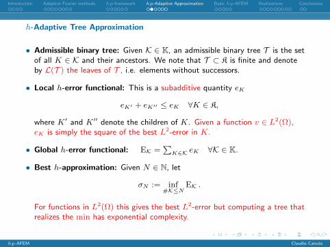
h-Adaptive Tree Approximation
• Admissible binary tree: Given K ∈ K, an admissible binary tree T is the setof all K ∈ K and their ancestors. We note that T ⊂ K is finite and denoteby L(T ) the leaves of T , i.e. elements without successors.
• Local h-error functional: This is a subadditive quantity eK
eK′ + eK′′ ≤ eK ∀K ∈ K,
where K′ and K′′ denote the children of K. Given a function v ∈ L2(Ω),eK is simply the square of the best L2-error in K.
• Global h-error functional: EK =∑K∈K eK ∀K ∈ K.
• Best h-approximation: Given N ∈ N, let
σN := inf#K≤N
EK .
For functions in L2(Ω) this gives the best L2-error but computing a tree thatrealizes the min has exponential complexity.
hp-AFEM Claudio Canuto
Introduction Adaptive Fourier methods hp-framework hp-Adaptive Approximation Basic hp-AFEM Realizations Conclusions
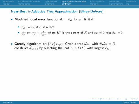
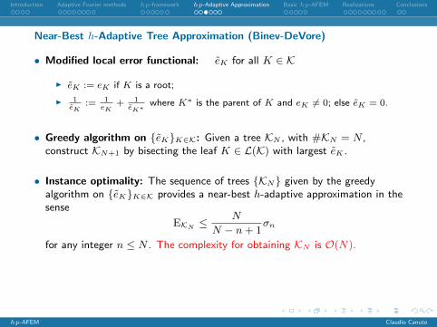
Near-Best h-Adaptive Tree Approximation (Binev-DeVore)
• Modified local error functional: eK for all K ∈ K
I eK := eK if K is a root;
I 1eK
:= 1eK
+ 1eK∗
where K∗ is the parent of K and eK 6= 0; else eK = 0.
• Greedy algorithm on eKK∈K: Given a tree KN , with #KN = N ,construct KN+1 by bisecting the leaf K ∈ L(K) with largest eK .
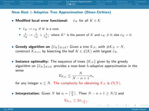
• Instance optimality: The sequence of trees KN given by the greedyalgorithm on eKK∈K provides a near-best h-adaptive approximation in thesense
EKN ≤N
N − n+ 1σn
for any integer n ≤ N . The complexity for obtaining KN is O(N).
• Interpretation: Given N let n = dN2e. Then N − n+ 1 ≥ N/2 and
EKN ≤ 2σdN2e.
hp-AFEM Claudio Canuto
Introduction Adaptive Fourier methods hp-framework hp-Adaptive Approximation Basic hp-AFEM Realizations Conclusions
Near-Best h-Adaptive Tree Approximation (Binev-DeVore)
• Modified local error functional: eK for all K ∈ K
I eK := eK if K is a root;
I 1eK
:= 1eK
+ 1eK∗
where K∗ is the parent of K and eK 6= 0; else eK = 0.
• Greedy algorithm on eKK∈K: Given a tree KN , with #KN = N ,construct KN+1 by bisecting the leaf K ∈ L(K) with largest eK .
• Instance optimality: The sequence of trees KN given by the greedyalgorithm on eKK∈K provides a near-best h-adaptive approximation in thesense
EKN ≤N
N − n+ 1σn
for any integer n ≤ N . The complexity for obtaining KN is O(N).
• Interpretation: Given N let n = dN2e. Then N − n+ 1 ≥ N/2 and
EKN ≤ 2σdN2e.
hp-AFEM Claudio Canuto
Introduction Adaptive Fourier methods hp-framework hp-Adaptive Approximation Basic hp-AFEM Realizations Conclusions
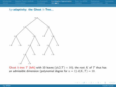
hp-adaptivity: the Ghost h-Tree...
and Subordinate hp-Tree (Binev)
10
6
2
1 1
4
3
2
1 1
1
1
4
1 3
2
1 1
1
10
6
2 4
3 1
4
1 3
2 1
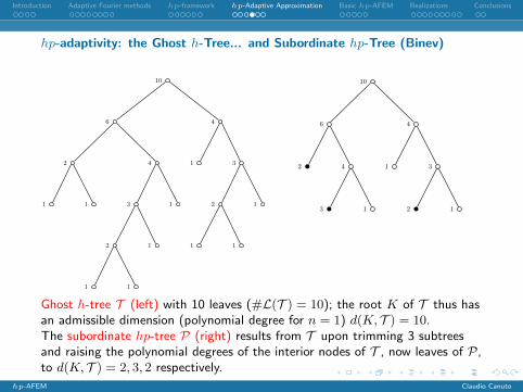
Ghost h-tree T (left) with 10 leaves (#L(T ) = 10); the root K of T thus hasan admissible dimension (polynomial degree for n = 1) d(K, T ) = 10.
The subordinate hp-tree P (right) results from T upon trimming 3 subtreesand raising the polynomial degrees of the interior nodes of T , now leaves of P,to d(K, T ) = 2, 3, 2 respectively.
hp-AFEM Claudio Canuto
Introduction Adaptive Fourier methods hp-framework hp-Adaptive Approximation Basic hp-AFEM Realizations Conclusions
hp-adaptivity: the Ghost h-Tree... and Subordinate hp-Tree (Binev)
10
6
2
1 1
4
3
2
1 1
1
1
4
1 3
2
1 1
1
10
6
2 4
3 1
4
1 3
2 1
Ghost h-tree T (left) with 10 leaves (#L(T ) = 10); the root K of T thus hasan admissible dimension (polynomial degree for n = 1) d(K, T ) = 10.The subordinate hp-tree P (right) results from T upon trimming 3 subtreesand raising the polynomial degrees of the interior nodes of T , now leaves of P,to d(K, T ) = 2, 3, 2 respectively.
hp-AFEM Claudio Canuto

Introduction Adaptive Fourier methods hp-framework hp-Adaptive Approximation Basic hp-AFEM Realizations Conclusions
Adaptive Strategy for hp-Refinements: hp-NEARBEST(Binev)
• Ghost h-tree T : This is the previous h-tree associated with v ∈ L2(Ω).
• Admissible dimension: Given K ∈ T , the dimension d(K, T ) is
d(K, T ) = #L(T (K)),
where T (K) is the subtree of T emanating from K. This quantity dependson both T and the underlying tree T .
• Local hp-error functionals: Let eK,d be the local error functional on K ∈ Twith polynomial dimension d. The modified local hp-error functional eK(T )reads
I eK(T ) := eK,1 provided K ∈ L(T ) is a leaf;
I eK(T ) := mineK′ (T ) + eK′′ (T ), eK,d(K,T )
otherwise.
• Subordinate hp-tree P: This tree is obtained from the h-tree uponeliminating the subtree T (K) whenever increasing the polynomial dimensionin K from 1 to d(K, T ) reduces the error, i.e.
eK(T ) = eK,d(K,T ).
hp-AFEM Claudio Canuto

Introduction Adaptive Fourier methods hp-framework hp-Adaptive Approximation Basic hp-AFEM Realizations Conclusions
Instance Optimality of hp-NEARBEST
• Theorem (Binev): The subordinate hp-tree PN with cardinality
#PN =∑
K∈L(PN )
d(K, TN ) = #L(TN ) = N
gives a hp partition DN with #DN = N and near-best hp-approximationover DN in the sense that the global error functional satisfies
EDN (v, f) ≤ 2N
N − n+ 1σn(v, f) ∀N ≥ n,
where σn is the best hp-error for (v, f) with n total degrees of freedom.
I The cost for constructing DN is bounded by O(∑
K∈TN d(K, TN )), and
varies from O(N logN) for well balanced trees to O(N2) for highlyunbalanced trees.
• Interpretation: Choosing B > 1, n = NB
and b = 12(1− 1
B) < 1 implies
I EDN (v, f) ≤ εI #DN ≤ B#D for all D ∈ D such that ED(v, f) ≤ bε.
hp-AFEM Claudio Canuto

Introduction Adaptive Fourier methods hp-framework hp-Adaptive Approximation Basic hp-AFEM Realizations Conclusions
Outline
Introduction
Adaptive Fourier methods
A framework for hp-Adaptivity
hp-Adaptive Approximation
Basic hp-Adaptive Algorithm
Realizations of the Algorithm
Conclusions
hp-AFEM Claudio Canuto

Introduction Adaptive Fourier methods hp-framework hp-Adaptive Approximation Basic hp-AFEM Realizations Conclusions
Basic Modules
We assume availability of the following routines, which realize the twofundamental steps of the algorithm.
I [D, fD] := hp-NEARBEST(ε, v, f)
The routine hp-NEARBEST takes as input ε > 0 and (v, f) ∈ V × F ,and outputs D ∈ D as well as fD, such that
(i) ED(v, f)12 ≤ ε;
(ii) #D ≤ B#D for any D ∈ D with ED(v, f)12 ≤ bε, for some constants
0 < b ≤ 1 ≤ B.
This routine may be implemented via Binev’s algorithm.
I [D, u] := PDE(ε,D, fD)
The routine PDE takes as input ε > 0, D ∈ Dc, and data fD ∈ FD. Itoutputs D ∈ Dc with D ≤ D and u ∈ V cD such that ‖u(fD)− u‖V ≤ ε.
hp-AFEM Claudio Canuto

Introduction Adaptive Fourier methods hp-framework hp-Adaptive Approximation Basic hp-AFEM Realizations Conclusions
Assumptions on Global Error Functional
We assume the existence of constants C1, C2 > 0 with
C1C2 < b,
such that the following properties hold:
• Continuity of the solution upon data:
‖u(f)− u(fD)‖V ≤ C1 infw∈V
ED(w, f)12 ∀D ∈ D, ∀ f ∈ F,
• Lipschitz continuity of ED upon state:
supf∈F|ED(w, f)
12 − ED(v, f)
12 | ≤ C2‖w − v‖V ∀D ∈ D, ∀v, w ∈ V.
hp-AFEM Claudio Canuto
Introduction Adaptive Fourier methods hp-framework hp-Adaptive Approximation Basic hp-AFEM Realizations Conclusions
Verifying the Assumptions on Global Error Functional
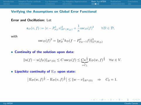
Error and Oscillation: Let
eD(v, f) := |v − P 1pDv|
2H1(KD) +
1
κoscD(f)2 ∀D ∈ D,
withoscD(f)2 = ‖p−1
D hD(f − P 0pD−1f)‖2L2(KD)
• Continuity of the solution upon data:
‖u(f)− u(fD)‖H1(Ω) ≤ C oscD(f) ≤ Cκ12︸ ︷︷ ︸
=C1
ED(w, f)12 ∀w ∈ V.
• Lipschitz continuity of ED upon state:∣∣ED(w, f)12 − ED(v, f)
12∣∣ ≤ ‖w − v‖H1(Ω) ⇒ C2 = 1.
• Bound on constants: C1C2 = Cκ12C2 < b for κ sufficiently small.
hp-AFEM Claudio Canuto

Introduction Adaptive Fourier methods hp-framework hp-Adaptive Approximation Basic hp-AFEM Realizations Conclusions
Verifying the Assumptions on Global Error Functional
Error and Oscillation: Let
eD(v, f) := |v − P 1pDv|
2H1(KD) +
1
κoscD(f)2 ∀D ∈ D,
withoscD(f)2 = ‖p−1
D hD(f − P 0pD−1f)‖2L2(KD)
• Continuity of the solution upon data:
‖u(f)− u(fD)‖H1(Ω) ≤ C oscD(f) ≤ Cκ12︸ ︷︷ ︸
=C1
ED(w, f)12 ∀w ∈ V.
• Lipschitz continuity of ED upon state:∣∣ED(w, f)12 − ED(v, f)
12∣∣ ≤ ‖w − v‖H1(Ω) ⇒ C2 = 1.
• Bound on constants: C1C2 = Cκ12C2 < b for κ sufficiently small.
hp-AFEM Claudio Canuto
Introduction Adaptive Fourier methods hp-framework hp-Adaptive Approximation Basic hp-AFEM Realizations Conclusions
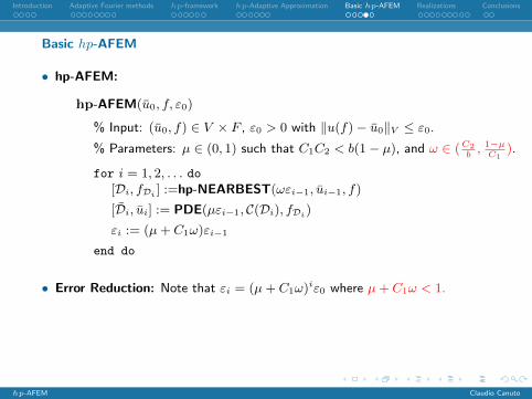
Basic hp-AFEM
• hp-AFEM:
hp-AFEM(u0, f, ε0)
% Input: (u0, f) ∈ V × F , ε0 > 0 with ‖u(f)− u0‖V ≤ ε0.
% Parameters: µ ∈ (0, 1) such that C1C2 < b(1− µ), and ω ∈ (C2b, 1−µC1
).
for i = 1, 2, . . . do[Di, fDi ] :=hp-NEARBEST(ωεi−1, ui−1, f)
[Di, ui] := PDE(µεi−1, C(Di), fDi)εi := (µ+ C1ω)εi−1
end do
• Error Reduction: Note that εi = (µ+ C1ω)iε0 where µ+ C1ω < 1.
• Coarsening: Tolerance for ui within PDE is τi := µεi−1 and the subsequentinput tolerance of hp-NEARBEST is ωεi = ω(µ+ C1ω)εi−1 > ωτi. Sincein our applications C2 = 1 and ω > C2/b ≥ 1, we see that ωεi > τi = µεi−1.
hp-AFEM Claudio Canuto

Introduction Adaptive Fourier methods hp-framework hp-Adaptive Approximation Basic hp-AFEM Realizations Conclusions
Basic hp-AFEM
• hp-AFEM:
hp-AFEM(u0, f, ε0)
% Input: (u0, f) ∈ V × F , ε0 > 0 with ‖u(f)− u0‖V ≤ ε0.
% Parameters: µ ∈ (0, 1) such that C1C2 < b(1− µ), and ω ∈ (C2b, 1−µC1
).
for i = 1, 2, . . . do[Di, fDi ] :=hp-NEARBEST(ωεi−1, ui−1, f)
[Di, ui] := PDE(µεi−1, C(Di), fDi)εi := (µ+ C1ω)εi−1
end do
• Error Reduction: Note that εi = (µ+ C1ω)iε0 where µ+ C1ω < 1.
• Coarsening: Tolerance for ui within PDE is τi := µεi−1 and the subsequentinput tolerance of hp-NEARBEST is ωεi = ω(µ+ C1ω)εi−1 > ωτi. Sincein our applications C2 = 1 and ω > C2/b ≥ 1, we see that ωεi > τi = µεi−1.
hp-AFEM Claudio Canuto
Introduction Adaptive Fourier methods hp-framework hp-Adaptive Approximation Basic hp-AFEM Realizations Conclusions
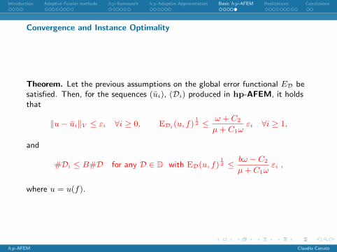
Convergence and Instance Optimality
Theorem. Let the previous assumptions on the global error functional ED besatisfied. Then, for the sequences (ui), (Di) produced in hp-AFEM, it holdsthat
‖u− ui‖V ≤ εi ∀i ≥ 0, EDi(u, f)12 ≤ ω + C2
µ+ C1ωεi ∀i ≥ 1,
and
#Di ≤ B#D for any D ∈ D with ED(u, f)12 ≤ bω − C2
µ+ C1ωεi ,
where u = u(f).
hp-AFEM Claudio Canuto

Introduction Adaptive Fourier methods hp-framework hp-Adaptive Approximation Basic hp-AFEM Realizations Conclusions
Outline
Introduction
Adaptive Fourier methods
A framework for hp-Adaptivity
hp-Adaptive Approximation
Basic hp-Adaptive Algorithm
Realizations of the Algorithm
Conclusions
hp-AFEM Claudio Canuto

Introduction Adaptive Fourier methods hp-framework hp-Adaptive Approximation Basic hp-AFEM Realizations Conclusions
A practical hp-adaptive algorithm
• Recall PDE:
I [D, u] := PDE(ε,D, fD)
The routine PDE takes as input ε > 0, D ∈ Dc, and data fD ∈ FD. Itoutputs D ∈ Dc with D ≤ D and u ∈ V cD such that ‖u(fD)− u‖V ≤ ε.
• Error reduction: For efficiency, PDE should exploit the work already carriedout within hp-AFEM.Precisely, for any desired error reduction factor % ∈ (0, 1), it should give
‖u(fD)− u‖V ≤ % infv∈V cD
‖u(fD)− v‖V .
• Indeed, at each call of PDE within hp-AFEM, we will be already guaranteedto have
infv∈V cD
‖u(fD)− v‖V ≤ Cε,
whence a suitable choice of % will yield
‖u(fD)− u‖V ≤ ε.• Remark: The input data fD is piecewise polynomial on the input partitionD, hence no data oscillation appears.
hp-AFEM Claudio Canuto

Introduction Adaptive Fourier methods hp-framework hp-Adaptive Approximation Basic hp-AFEM Realizations Conclusions
A practical hp-adaptive algorithm
• Recall PDE:
I [D, u] := PDE(ε,D, fD)
The routine PDE takes as input ε > 0, D ∈ Dc, and data fD ∈ FD. Itoutputs D ∈ Dc with D ≤ D and u ∈ V cD such that ‖u(fD)− u‖V ≤ ε.
• Error reduction: For efficiency, PDE should exploit the work already carriedout within hp-AFEM.Precisely, for any desired error reduction factor % ∈ (0, 1), it should give
‖u(fD)− u‖V ≤ % infv∈V cD
‖u(fD)− v‖V .
• Indeed, at each call of PDE within hp-AFEM, we will be already guaranteedto have
infv∈V cD
‖u(fD)− v‖V ≤ Cε,
whence a suitable choice of % will yield
‖u(fD)− u‖V ≤ ε.
• Remark: The input data fD is piecewise polynomial on the input partitionD, hence no data oscillation appears.
hp-AFEM Claudio Canuto

Introduction Adaptive Fourier methods hp-framework hp-Adaptive Approximation Basic hp-AFEM Realizations Conclusions
A practical hp-adaptive algorithm
• Recall PDE:
I [D, u] := PDE(ε,D, fD)
The routine PDE takes as input ε > 0, D ∈ Dc, and data fD ∈ FD. Itoutputs D ∈ Dc with D ≤ D and u ∈ V cD such that ‖u(fD)− u‖V ≤ ε.
• Error reduction: For efficiency, PDE should exploit the work already carriedout within hp-AFEM.Precisely, for any desired error reduction factor % ∈ (0, 1), it should give
‖u(fD)− u‖V ≤ % infv∈V cD
‖u(fD)− v‖V .
• Indeed, at each call of PDE within hp-AFEM, we will be already guaranteedto have
infv∈V cD
‖u(fD)− v‖V ≤ Cε,
whence a suitable choice of % will yield
‖u(fD)− u‖V ≤ ε.• Remark: The input data fD is piecewise polynomial on the input partitionD, hence no data oscillation appears.
hp-AFEM Claudio Canuto

Introduction Adaptive Fourier methods hp-framework hp-Adaptive Approximation Basic hp-AFEM Realizations Conclusions
• PDE: This module may be implemented by the usual loop
SOLVE → ESTIMATE → MARK → GROW
where
GROW may be either an h-refinement or a p-enrichment.
• Features:
I ESTIMATE: should be based on a reliable and efficient a posteriori errorindicator, with constants independent of the current hp-partition D(in particular, “p-robust”).
I GROW: should yield a new hp partition Dnew with #Dnew . #D andguaranteed saturation property
‖u− uD‖V . ‖uDnew − uD‖V(all constants independent of D).
I MARK: might be skipped. Indeed, since the task of producing a near-besthp-partition is assigned to hp-NEARBEST, in principle even a uniformrefinement/enrichment is allowed.
hp-AFEM Claudio Canuto
Introduction Adaptive Fourier methods hp-framework hp-Adaptive Approximation Basic hp-AFEM Realizations Conclusions
Applications to elliptic self-adjoint problems
We detail three possible realizations of PDE, based on:
I a residual estimator, in dimension 1,
I a residual estimator, in dimension 2
I an equilibrated flux estimator, in dimension 2.
• In a 1D domain, for the general elliptic self-adjoint problem
u ∈ H10 (Ω) : −(µux)x + σu = f + gx in H−1(Ω),
I the residual-based error estimator ηD(uD, fD) defined by
η2D(uD, fD) =
∑D∈D
‖rD‖2H−1(KD)
is p-robust and easily computable element-wise;
I the saturation property is guaranteed by raising the polynomial degree frompD to some pD ≤ 2pD + 3 in each marked element.
I Thus, hp-AFEM is fully optimal.
hp-AFEM Claudio Canuto
Introduction Adaptive Fourier methods hp-framework hp-Adaptive Approximation Basic hp-AFEM Realizations Conclusions
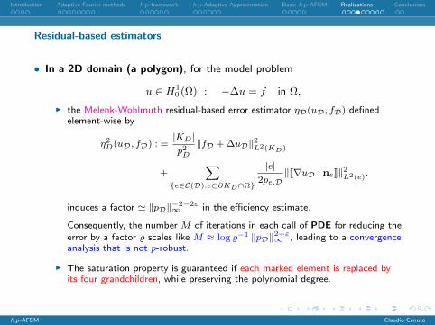
Residual-based estimators
• In a 2D domain (a polygon), for the model problem
u ∈ H10 (Ω) : −∆u = f in Ω,
I the Melenk-Wohlmuth residual-based error estimator ηD(uD, fD) definedelement-wise by
η2D(uD, fD) : =
|KD|p2D
‖fD + ∆uD‖2L2(KD)
+∑
e∈E(D):e⊂∂KD∩Ω
|e|2pe,D
‖[[∇uD · ne]]‖2L2(e).
induces a factor ' ‖pD‖−2−2ε∞ in the efficiency estimate.
Consequently, the number M of iterations in each call of PDE for reducing theerror by a factor % scales like M ≈ log %−1 ‖pD‖2+ε
∞ , leading to a convergenceanalysis that is not p-robust.
I The saturation property is guaranteed if each marked element is replaced byits four grandchildren, while preserving the polynomial degree.
hp-AFEM Claudio Canuto
Introduction Adaptive Fourier methods hp-framework hp-Adaptive Approximation Basic hp-AFEM Realizations Conclusions
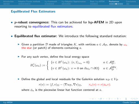
Equilibrated Flux Estimators
• p-robust convergence: This can be achieved for hp-AFEM in 2D uponresorting to equilibrated flux estimators.
• Equilibrated flux estimator: We introduce the following standard notation:
I Given a partition D made of triangles K, with vertices a ∈ AD, denote by ωathe star (or patch) of elements containing a.
I For any such vertex, define the local energy space
H1∗(ωa) :=
v ∈ H1(ωa) : 〈v, 1〉ωa = 0 a ∈ Aint
D ,
v ∈ H1(ωa) : v = 0 on ∂ωa ∩ ∂Ω a ∈ AbdryD .
I Define the global and local residuals for the Galerkin solution uD ∈ VDr(v) := 〈f, v〉Ω − 〈∇uD,∇v〉Ω, ra(v) = r(φav).
where φa is the piecewise linear hat function centered at a.
hp-AFEM Claudio Canuto

Introduction Adaptive Fourier methods hp-framework hp-Adaptive Approximation Basic hp-AFEM Realizations Conclusions
p-Robust A Posteriori Estimates
• Upper and lower bounds:
‖∇(u−uD)‖2Ω ≤ 3∑a∈AD
‖ra‖2H1∗(ωa)′ , ‖ra‖H1
∗(ωa)′ . ‖∇(u−uD)‖ωa ∀a ∈ AD.
• p-robust equivalence:
‖ra‖H1∗(ωa)′ ' ‖σa‖ωa
where σa ∈ RT (Da) is a suitable equilibrated flux for uD (i.e., it satisfies〈∇ · σa, 1〉T = 〈f, 1〉T for all T ⊂ ωa),[Braess, Pillwein and Schoberl (2009)]
• Computability. A particular equilibrated flux σa can be efficiently computedby solving a discrete saddle-point problem in the space RT (Da).[Ern and Vohralık (2015)]
hp-AFEM Claudio Canuto
Introduction Adaptive Fourier methods hp-framework hp-Adaptive Approximation Basic hp-AFEM Realizations Conclusions
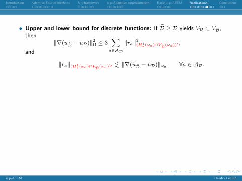
• Upper and lower bound for discrete functions: If D ≥ D yields VD ⊂ VD,then
‖∇(uD − uD)‖2Ω ≤ 3∑a∈AD
‖ra‖2(H1∗(ωa)∩VD(ωa))′ ,
and
‖ra‖(H1∗(ωa)∩VD(ωa))′ . ‖∇(uD − uD)‖ωa ∀a ∈ AD.
• Marking: Suppose we apply a star-based Dorfler marking, and that for anymarked star we can find a local space VD(ωa) ⊃ VD(ωa) for which it holds
‖ra‖H1∗(ωa)′ . ‖ra‖(H1
∗(ωa)∩VD(ωa))′ uniformly in p.
• Saturation property: Then, we immediately obtain the p-robust saturationproperty
‖∇(u− uD)‖2Ω . ‖∇(uD − uD)‖2Ω
• Contraction property: This implies the following bound with % < 1
‖∇(u− uD)‖Ω ≤ %‖∇(u− uD)‖Ω
hp-AFEM Claudio Canuto

Introduction Adaptive Fourier methods hp-framework hp-Adaptive Approximation Basic hp-AFEM Realizations Conclusions
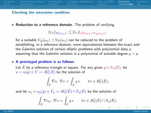
Checking the saturation condition
• Reduction to a reference domain. The problem of verifying
‖ra‖H1∗(ωa)′ . ‖ra‖(H1
∗(ωa)∩VD(ωa))′
for a suitable VD(ωa) ⊃ VD(ωa) can be reduced to the problem ofestablishing, in a reference domain, norm equivalences between the exact andthe Galerkin solution of certain elliptic problems with polynomial data p,assuming that the Galerkin solution is a polynomial of suitable degree q > p.
• A prototypal problem is as follows:
Let E be a reference triangle or square. For any given g ∈ Pp(E), letu = u(g) ∈ V := H1
0 (E) be the solution of∫E
∇u · ∇v =
∫E
g v ∀v ∈ H10 (E),
and let uq = uq(g) ∈ Vq := H10 (E) ∩ Pq(E) be the solution of∫
E
∇uq · ∇v =
∫E
g v ∀v ∈ H10 (E) ∩ Pq(E).
hp-AFEM Claudio Canuto
Introduction Adaptive Fourier methods hp-framework hp-Adaptive Approximation Basic hp-AFEM Realizations Conclusions
Checking the saturation condition
• Reduction to a reference domain. The problem of verifying
‖ra‖H1∗(ωa)′ . ‖ra‖(H1
∗(ωa)∩VD(ωa))′
for a suitable VD(ωa) ⊃ VD(ωa) can be reduced to the problem ofestablishing, in a reference domain, norm equivalences between the exact andthe Galerkin solution of certain elliptic problems with polynomial data p,assuming that the Galerkin solution is a polynomial of suitable degree q > p.
• A prototypal problem is as follows:
Let E be a reference triangle or square. For any given g ∈ Pp(E), letu = u(g) ∈ V := H1
0 (E) be the solution of∫E
∇u · ∇v =
∫E
g v ∀v ∈ H10 (E),
and let uq = uq(g) ∈ Vq := H10 (E) ∩ Pq(E) be the solution of∫
E
∇uq · ∇v =
∫E
g v ∀v ∈ H10 (E) ∩ Pq(E).
hp-AFEM Claudio Canuto

Introduction Adaptive Fourier methods hp-framework hp-Adaptive Approximation Basic hp-AFEM Realizations Conclusions
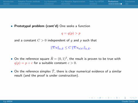
• Prototypal problem (cont’d) One seeks a function
q = q(p) > p
and a constant C > 0 independent of g and p such that
‖∇u‖0,E ≤ C ‖∇uq(p)‖0,E .
• On the reference square R = (0, 1)2, the result is proven to be true withq(p) = p+ c for a suitable constant c > 0.
• On the reference simplex T , there is clear numerical evidence of a similarresult (and the proof is under construction).
hp-AFEM Claudio Canuto
Introduction Adaptive Fourier methods hp-framework hp-Adaptive Approximation Basic hp-AFEM Realizations Conclusions
• Prototypal problem (cont’d) One seeks a function
q = q(p) > p
and a constant C > 0 independent of g and p such that
‖∇u‖0,E ≤ C ‖∇uq(p)‖0,E .
• On the reference square R = (0, 1)2, the result is proven to be true withq(p) = p+ c for a suitable constant c > 0.
• On the reference simplex T , there is clear numerical evidence of a similarresult (and the proof is under construction).
hp-AFEM Claudio Canuto

Introduction Adaptive Fourier methods hp-framework hp-Adaptive Approximation Basic hp-AFEM Realizations Conclusions
Outline
Introduction
Adaptive Fourier methods
A framework for hp-Adaptivity
hp-Adaptive Approximation
Basic hp-Adaptive Algorithm
Realizations of the Algorithm
Conclusions
hp-AFEM Claudio Canuto
Introduction Adaptive Fourier methods hp-framework hp-Adaptive Approximation Basic hp-AFEM Realizations Conclusions
Conclusions
• We have considered several adaptive spectral methods, with guaranteedlinear or quadratic convergence; we have discussed their optimality propertiesin terms of cardinality of activated degrees of feedom.
• We have introduced an abstract framework for hp-adaptivity.
• We have presented an algorithm for hp-adaptive approximation, withinstance optimality.
• We have considered a general, convergent and nearly-optimal hp-adaptivefinite element method, and we have discussed several specific realizations.
• Various extension are waiting:
I Discontinuous Galerkin (underway)I Stokes systemI anisotropic adaptivityI non-symmetric operatorsI ...
hp-AFEM Claudio Canuto

Introduction Adaptive Fourier methods hp-framework hp-Adaptive Approximation Basic hp-AFEM Realizations Conclusions
Some references
I C. Canuto, R.H. Nochetto and M. Verani, Adaptive Fourier-Galerkin Methods,Math. Comp. 83 (2014), 1645–1687.
I C. Canuto, R.H. Nochetto and M. Verani, Contraction and optimality propertiesof adaptive Legendre-Galerkin methods: the 1-dimensional case, Comput. &Math. with Appl. 67 (2014), no.4, 752–770.
I C. Canuto, V. Simoncini and M. Verani, On the decay of the inverse of matricesthat are sum of Kronecker products, Linear Algebra Appl., 452 (2014), 21–39
I C. Canuto, V. Simoncini and M. Verani, Adaptive Legendre-Galerkin methods:the multidimensional case, J. Sci. Comput. 63 (2015), 769–798
I C. Canuto, R.H. Nochetto, R. Stevenson, M. Verani, Adaptive spectral Galerkinmethods with dynamic marking, SIAM J. Numer. Anal. 54 (2016), 3193–3213
I C. Canuto, R.H. Nochetto, R. Stevenson, M. Verani, Convergence and optimalityof hp-AFEM, Numer. Math. 135 (2017), 1073-1119
I C. Canuto, R.H. Nochetto, R. Stevenson, M. Verani, On p-robust saturation forhp-AFEM, Comput. & Math. with Appl. 73 (2017), 2004–2022
hp-AFEM Claudio Canuto