adaptive myelination and its synchronous dynamics in the
TRANSCRIPT

Adaptive myelination and its synchronous dynamics in theKuramoto network model with state-dependent delays
by
Seong Hyun Park
A thesis submitted in conformity with the requirementsfor the degree of Doctor of Philosophy
Graduate Department of Department of MathematicsUniversity of Toronto
© Copyright 2021 by Seong Hyun Park


Adaptive myelination and its synchronous dynamics in the Kuramoto networkmodel with state-dependent delays
Seong Hyun ParkDoctor of Philosophy
Graduate Department of Department of MathematicsUniversity of Toronto
2021
Abstract
White matter pathways form a complex network of myelinated axons that play
a critical role in brain function by facilitating the timely transmission of neural
signals. Recent evidence reveals that white matter networks are adaptive and that
myelin undergoes continuous reformation through behaviour and learning during
both developmental stages and adulthood in the mammalian lifecycle. Conse-
quently, this allows axonal conduction delays to adjust in order to regulate the
timing of neuron signals propagating between different brain regions. Despite its
newly founded relevance, the network distribution of conduction delays have yet
to be widely incorporated in computational models, as the delays are typically
assumed to be either constant or ignored altogether. From its clear influence to-
wards temporal dynamics, we are interested in how adaptive myelination affects
oscillatory synchrony in the brain. We introduce a plasticity rule into the de-
lays of a weakly coupled oscillator network, whose positions relative to its natural
limit cycle oscillations is described through a coupled phase model. From this,
the addition of slowly adaptive network delays can potentially lead coupled os-
cillators to a more phase synchronous limit cycle. To see how adaptive white
matter remodelling can shape synchronous dynamics, we modify the canonical
Kuramoto model by enabling all connections with phase-dependent delays that
change over time. We directly compare the synchronous behaviours of the Ku-
ramoto model equipped with static delays and adaptive delays by analyzing the
synchronized equilibria and stability of the system’s phases. Our mathematical
analysis of the model with dirac and exponentially distributed connection de-
lays, supported by numerical simulations, demonstrates that larger, more widely
ii

varying distributions of delays generally impede synchronization in the Kuramoto
network. Adaptive delays act as a stabilizing mechanism for the synchrony of the
network by adjusting towards a more optimal distribution of delays. Adaptive
delays also make global synchronization more resilient to perturbations and injury
towards network architecture. Our results provide insights about the potential
significance of activity-dependent myelination. For future works, we hope that
these results lay out the groundwork to computationally study the influence of
adaptative myelination towards large-scale brain synchrony.
iii

Dedicated to my parents, who have always supported me,
and
to my brother, Kevin, who will always be my closest friend and family.
iv

Acknowledgments
It has been a long and arduous journey for me to finish this dissertation, and I
couldn’t have done it without the help of the wonderful people around me. I would
like to devote this page to thank everyone who was involved.
First and foremost, I would like to thank my parents for all their time and
efforts to ensure that I can focus on my studies. To mom and dad, I owe so much
to your continuous support, and I hope to keep making you guys proud. To my
brother Kevin, I have always been able to open up and share my thoughts with
you, and you listened to me every time. I couldn’t be more fortunate to have you
in my life.
I would like to thank the people of the U of T mathematics department for
allowing me to graduate. I would especially like to thank the graduate secretary
Jemima for her guidance and consultation. If it weren’t for you, I wouldn’t have
been able to find an awesome supervisor and graduate.
I would like to thank my advisor, Jeremie Lefebvre, for taking me in as his
doctoral student 3 years back. You gave me more chances than I deserved, and
you invested your time to regularly meet with me despite your busy and often
hectic schedule. You’ve helped me non-stop from start to finish, and I couldn’t
have asked for a better advisor.
I would like to thank the Krembil Computational Neuroscience lab, for inspiring
me and teaching me a ton of things, especially the neurobiology that I initially
had no familiarity with. I feel incredibly previliged to be around such a welcoming
and dedicated community, and I hope that many more students get involved in
neuroscience during the years to come.
Special thanks to Adam Stinchcombe for your invaluable feedback on the nu-
merics. The figures wouldn’t be half as good without your input.
And with that, I look forward to entering a new chapter of my life. But I will
forever cherish the years I spent during these graduate years.
v

Statement of originality
Unless cited, the work and results presented in this paper are the product of the
author’s original research. Chapter 1 overviews the physiological concepts of neu-
ronal oscillations and myelin plasticity, and ties them into the paper’s hypothesis
on neurocomputational models. Chapter 2 introduces the weakly coupled oscil-
lator network model and phase model with connection delays, and establishes
the projective relation between the two models. Chapter 3 defines the Kuramoto
phase model with constant delays, and derives the equations for an N -dimensional
oscillator network’s synchronous state and its respective stability criteria. Chapter
4 analyzes the Kuramoto phase model with adaptive delays. The full contents of
Chapter 4 is published as the journal ‘Synchronization and resilience in the Ku-
ramoto white matter network model with adaptive state-dependent delays’ in the
Journal of Mathematical Neuroscience (2020). The original model was proposed
by co-author Jeremie Lefebvre, and all analysis and numerical experiments were
conducted by first author Seong Hyun Park. Chapter 5 analyzes the Kuramoto
phase model with adaptive conduction velocities. The model used in Chapter 5
is taken from the research article ‘Activity-dependent myelination: a glial mech-
anism of oscillatory self-organization in large-scale brain networks’ published in
PNAS (2020) by Rabiya Noori, Jeremie Lefebvre, Seong Hyun Park et al. Chap-
ter 5.1 defines the model and its physiological meaning, and the contents are fully
taken, with permission from co-author Jeremie Lefebvre, from the research arti-
cle. Chapter 5.2 derives theoretical equations which can be found in the research
article. Chapter 5.3 conducts numerical experiments on the model, and all con-
tents in this section are entirely original research conducted by Seong Hyun Park
and is not published in the research article. Chapter 6 concludes the findings of
this dissertation. Appendix A discusses the persistent entrainment property of a
mean-field model, as published as the research article ‘Persistent Entrainment in
Non-linear Neural Networks With Memory’ by Seong Hyun Park, Jeremie Lefeb-
vre et al. in Frontiers in Applied Mathematics and Statistics (2018). The contents
of this Appendix chapter is considered to be separate from the main dissertation
vi

topic. All analysis and results found in this section is published in the research
article and is the original contribution of first author Seong Hyun Park.
vii

Contents
1 Introduction 1
1.1 The neuron . . . . . . . . . . . . . . . . . . . . . . . . . . . . . . . 2
1.2 Measuring and modeling neuronal outputs . . . . . . . . . . . . . . 9
1.3 Oscillations and synchrony . . . . . . . . . . . . . . . . . . . . . . . 12
1.4 Myelin and white matter plasticity . . . . . . . . . . . . . . . . . . 16
1.5 Understanding the link between adaptive myelination and neural
synchrony . . . . . . . . . . . . . . . . . . . . . . . . . . . . . . . . 21
2 Delay oscillator models 27
2.1 Weakly coupled oscillator networks with connection delays . . . . . 28
2.2 Phase models and synchrony . . . . . . . . . . . . . . . . . . . . . . 32
2.3 Malkin’s theorem . . . . . . . . . . . . . . . . . . . . . . . . . . . . 36
2.4 Formulation of adaptive delays . . . . . . . . . . . . . . . . . . . . . 42
2.5 Summary . . . . . . . . . . . . . . . . . . . . . . . . . . . . . . . . 46
3 Kuramoto network model with distributed delays 47
3.1 Derivation of model . . . . . . . . . . . . . . . . . . . . . . . . . . . 47
3.2 The synchronous state . . . . . . . . . . . . . . . . . . . . . . . . . 49
3.3 Synchrony with single delay . . . . . . . . . . . . . . . . . . . . . . 52
3.4 Synchrony with distributed delays . . . . . . . . . . . . . . . . . . . 57
3.5 Synchrony with exponentially distributed delays . . . . . . . . . . . 61
3.6 The incoherent state . . . . . . . . . . . . . . . . . . . . . . . . . . 66
3.7 Numerical simulations for single and exponentially distributed delays 71
3.8 Summary . . . . . . . . . . . . . . . . . . . . . . . . . . . . . . . . 76
viii

4 Kuramoto model with adaptive delays 77
4.1 Modeling adaptive delays . . . . . . . . . . . . . . . . . . . . . . . . 77
4.2 Synchronized state and stability with plastic delays . . . . . . . . . 79
4.3 Synchronization of two coupled oscillators with plastic delays . . . . 83
4.4 Synchronization in large-scale oscillator networks with plastic delays 86
4.5 Numerical simulations for networks with adaptive delays . . . . . . 92
4.6 Application: resilience to injury with sparse connectivity . . . . . . 97
4.7 Summary . . . . . . . . . . . . . . . . . . . . . . . . . . . . . . . . 101
5 Kuramoto model with adaptive conduction velocities 103
5.1 Modeling adaptive velocities . . . . . . . . . . . . . . . . . . . . . . 103
5.2 Impact on synchronization . . . . . . . . . . . . . . . . . . . . . . . 105
5.3 Numerical simulations . . . . . . . . . . . . . . . . . . . . . . . . . 107
5.4 Summary . . . . . . . . . . . . . . . . . . . . . . . . . . . . . . . . 111
6 Discussion 113
6.1 Summary and relevance of results . . . . . . . . . . . . . . . . . . . 113
6.2 Limitations . . . . . . . . . . . . . . . . . . . . . . . . . . . . . . . 116
6.3 Future directions . . . . . . . . . . . . . . . . . . . . . . . . . . . . 120
A Persistent entrainment in non-linear neural networks 125
B Proof of theorems 133
C Smooth adjustments to functions 137
D Numerical Methods 141
List of symbols 143
Bibliography 145
ix

List of Figures
1.1 Illustration of sodium (Na+) and potassium (K+) protein
channels. The movement of ions is moderated by the opening
and closing of the channel gates. When their respective gates are
opened, diffusion forces cause Na+ ions to flow into the cell and K+
ions to flow outward. Illustration taken from [3] . . . . . . . . . . . 3
1.2 Illustration of forces created by concentration differences.
The specific permeability of the cell membrane prevents the ions
from distributing evenly along the two sides of the membrane, lead-
ing to a concentration difference of cations and anions. This causes
an electrostatic force and diffusion force to act on the cell mem-
brane. Illustration taken from [63] . . . . . . . . . . . . . . . . . . . 4
1.3 Graph of a typical action potential cycle. The labeled graph
shows the corresponding changes of the membrane potential (in
millivolts) at each phase of the action potential cycle (resting, de-
polarization, repolarization, refractory period) over time. For illus-
trative clarity, we plot our own numerically simulated values for the
voltage graph using the Hudgkin-Huxley model, which we will be
presented in Section 1.2. . . . . . . . . . . . . . . . . . . . . . . . . 5
x
1.4 Anatomy of neuronal signaling circuitry. A. The neuron re-
ceives signals through its dendrite branches, and fires signals along
the axon to other neurons. B. The anatomy of the synapse. Neuro-
transmitters are released from activated vesicles, where they make
way along the synaptic junction and latch onto the receptor pro-
teins. Original illustration taken from [3]. . . . . . . . . . . . . . . . 8
1.5 Extracellular EEG and MEG recordings. Recordings of a
drug-resistant epilepsy patient. A. Simultaneous recordings from
depth, grid, and scalp electrodes over a 4s (left column) and 6s
(right column) epoch. B. MEG recording (blue) alongside a depth
EEG placed in the hippocampus (red). The original figure and
additional details can be found in [11]. . . . . . . . . . . . . . . . . 10
1.6 Computational models of a neuron’s membrane potential.
A. Membrane voltage (mV) over time using the Hodgkin-Huxley
equations, found in [28]. B. Membrane voltage (mV) of a single
neuron, using the stochastic spiking model with 800 excitatory neu-
rons and 200 inhibitory neurons. The algorithm used for the spik-
ing model can be found in [36]. The resting potentials (RP) of each
model is also plotted. . . . . . . . . . . . . . . . . . . . . . . . . . . 12
1.7 Interpretation of phases from spiking activity. A. Membrane
voltage (mV) over time using the Hodgkin-Huxley equations, found
in [28]. The membrane potential peaks occur at a fixed interval
following t > 10ms. The consecutive peak times t1, t2 define the
period T = t2 − t1. B. Phase model θ(t) of the Hodgkin-Huxley
peak times in plot A, graphed as a sine wave such that the times
t at which sin(θ(t)) = 1 align with the spike times. Here, θ(t) is
defined such that θ(tk) = 2πk + φ for each spike time tk and some
constant phase-offset φ chosen so that the peaks align, with linear
interpolation of θ(t) on each interval t ∈ [tk, tk+1]. . . . . . . . . . . 15
xi

1.8 Anatomy of a myelinated axon. Mature oligodendrocyte cells
form myelinated sheaths that insulate segments of an axonal path,
as an extended glial plasma membrane wraps around the axonal
cord spirally and compacts. Action potential signals travel along
myelinated segments through saltatory conduction, which is a far
more efficient and quicker method of propagation. The gaps be-
tween myelinated segments/internodes are the nodes of Ranvier, at
which the action potential is replenished. The complete diagram is
taken from [16]. . . . . . . . . . . . . . . . . . . . . . . . . . . . . . 19
1.9 Diagram illustrating the influence of conduction velocities
towards spike arrival times. Two neurons F1 and F2 fire spikes
at time t1 and t2 towards a single target neuron T . The signals
propagate at different conduction speeds v1 and v2 for F1 and F2
respectively, from which the signals arrive at times t1 + d1/v1 and
t2 +d2/v2. The arrival times may differ, unless v1 and v2 correspond
to the heterogeneous distances d1 and d2. Here, d1 > d2, and hence
it is ideal for v1 < v2 for the arrival times to match. Illustration
taken and adjusted from [54]. . . . . . . . . . . . . . . . . . . . . . 22
2.1 Schematic of phase parameterization of limit cycle trajec-
tory. The phase variable θ(t) indicates the relative position of
oscillator x(t) along 2π-periodic limit cycle γ at time t. . . . . . . . 34
xii

2.2 Diagram illustrating adaptation towards a more synchronous
periodic trajectory. Here, M = γ1 × · · · × γN is the manifold
with natural limit cycles γi corresponding to the uncoupled net-
work (2.3). On M , the oscillators have a phase of ω0t at time t.
There are two invariant manifolds Mε(τ0), Mε(τ
∗) nearby M cor-
responding to the coupled network (2.2) with initial delays τ 0 and
modified delays τ ∗ respectively. The arrows represent the oscilla-
tors’ phase positions θi(t) along each manifold trajectory. Here,
Mε(τ0) (orange) lacks in-phase synchrony with the phase positions
spread out, whereas Mε(τ∗) (green) is nearly in-phase and hence
shows more coherent synchronization. A shift in delays τ 0 → τ ∗
can attract the oscillators from Mε(τ0) to Mε(τ
∗). . . . . . . . . . . 45
3.1 Theoretical stability plots for the Kuramoto network with
single static delay. A. The L-H error curve of fixed point equation
(3.13) for the in-phase sync. frequency Ω. There are three sync.
frequencies Ω1 < Ω2 < Ω3 on the interval [ω0 − g, ω0 + g]. B. Plot
of cos(Ωiτ0) for each sync. frequency Ωi, i = 1, 2, 3 in reference to
plot A. Frequencies whose markers are above the x-axis (red line)
indicates that the sync. state is stable, and unstable otherwise. C,
D, E. Complex scatter plots of the exact stability eigenvalues for
frequencies Ω1, Ω2, Ω3 respectively, using the LambertW equation
(3.19) for branch indices k ∈ Z, |k| ≤ 10. With each frequency,
the distribution of eigenvalues is consistent with the stability deter-
mined by cos(Ωτ 0). For all plots, the all-to-all topology aij = 1 is
used, and ω0 = 1.0, g = 1.5, τ 0 = 2.0s. . . . . . . . . . . . . . . . . 55
xiii

3.2 Stability plots for the Kuramoto network with increasing
coupling and increasing single delay. A. Plot of all sync. fre-
quencies satisfying (3.13) for varying coupling coefficient g > 0 and
fixed delay τ 0 = 2.0s. B. The respective stability criterion plots
cos(Ωτ 0) of each frequency Ω found in plot A. At every g > 0, each
frequency’s stability criterion is plotted using the same colour. C.
Plot of all sync. frequencies satisfying (3.13) for varying delay τ 0
and fixed coupling g = 0.15. D. The respective stability plot of each
frequency Ω found in plot C. For all plots, the all-to-all topology
aij = 1 is used, and ω0 = 1.0. . . . . . . . . . . . . . . . . . . . . . 56
3.3 Stability plots for the Kuramoto network with exponen-
tially sampled delays. A. Plot of the single sync. frequency Ω
satisfying (3.40) with respect to each increasing mean delay τm. B.
Plot of the real (magenta) and imaginary (green) parts of the two
non-zero expected eigenvalues λ1 (x marker), λ2 (square marker)
from (3.43) at each τm. C. Plot of stability criterions with increas-
ing τm at the single sync. frequency as shown in plot A. The purple
line plots sup Re(Λ) at each τm (purple), where Λ is the set of lo-
cated eigenvalues near λ = 0 that satisfy (3.29) with respect to an
instance of sampled i.i.d. delays τij ∼ exp(τm). There is a loss of
stability as sup Re(Λ) becomes positive near the critical mean delay
τm = τmc . The orange line plots − cos(Ωτm). Positive values im-
ply instability around frequency Ω. D, E. Complex plots showing
the expected (blue) eigenvalues and actual (red) eigenvalues Λ, in
accordance to a sampled set of exponential delays τij with mean
τm = 2.0s, 6.0s and respective sync. frequency Ω. For all plots,
N = 60 with the all-to-all topology aij = 1, and g = 1.5, ω0 = 1.0. . 63
xiv

3.4 Expected value and standard deviations of the eigenvalue
matrix det[Ψλ,N ]. A. Plot of the theoretical mean and standard
deviation µλ (blue), σλ (red) from (3.37) with increasing τm at fixed
λ = 0.1. Here, µλ, σλ is normalized by multiplication factor βλ.
B, C. Plots of µλ (blue line), σλ (red line) at fixed τm = 2.0s, 6.0s
respectively while taking the limit λ→ 0 (or as − log10 λ increases).
At τm = 2.0s, the inequality µλ > σλ holds for all small values λ
near λ = 0+. At τm = 6.0s, the inequality µλ σλ holds and
σλ increases as λ → 0+. D. Plot of the (scaled by log10) standard
deviation of the eigenvalue matrix Ψλ,N at each decreasing λ→ 0+
and fixed τm = 2.0s (purple x), τm = 6.0s (magenta square). E.
The p-value of the lillietest for normality of det[Ψλ,N ] at each λ as
λ → 0 at τm = 2.0s (green) and τm = 6.0s (black). A small p-
value rejects the null hypothesis and implies lack of normality. The
values in plots D, E were obtained by taking the sample variance
and p-value of det[Ψλ,N ] computed over 2000 iterations of sampled
delays τij with exponential mean τm. For all plots, N = 60 with
the all-to-all topology aij = 1, and g = 1.5, ω0 = 1.0. . . . . . . . . 66
xv

3.5 Stability plots for the incoherent state of the Kuramoto
network. A. Plot of the stability regions instability regions for the
incoherent state and the synchronous state of the Kuramoto model
with respect to single delay τ 0 and coupling coefficient g > 0. The
red area is the unstable region for the synchronous state θi(t) = Ωt
with the red curve g = g(τ 0), τ 0 > 0 as defined by (3.23), while the
blue + red region is the neutrally stable region for the incoherent
state with the blue curve g = 2 g(τ 0), τ 0 > 0. B. Plots of the real
part of the two eigenvalues λ1, λ2 describing the stability around
the incoherent state with exponentially distributed delays, scaled
by s. log10(x) defined by (3.45). The positive eigenvalue branch
Re(λ1) > 0 (red) and negative eigenvalue branch Re(λ2) < 0 (green)
are plotted with increasing mean delay τm. Here, g = 1.5. For both
plots, the all-to-all topology aij = 1 is used and ω0 = 1.0. . . . . . . 70
3.6 Numerical plots over time for the Kuramoto model with
single delay. A, B. Plot of the instantaneous frequencies θ′i(t)
and (sine) phase deviations φi(t) over time of a trial with g = 1.0,
τ 0 = 4.0s. We observe that in-phase synchronization occurs for
this trial. C, D. Likewise plots over time of a trial with g = 0.2,
τ 0 = 2.5s. We observe that entrainment occurs, but the synchrony
is not in-phase. E. The order parameter of the two trials plotted
in A, B (orange) and C, D (blue). Each trial was run up to time
T = 300s. The parameters used were N = 20 with the all-to-all
topology aij = 1, and ω0 = 1.0. . . . . . . . . . . . . . . . . . . . . 72
xvi

3.7 Numerical plots for asymptotic values of the Kuramoto
model with single delay. A. Heatmap of the asymptotic sync.
frequencies Ω of different trials with parameters g ∈ [0, 1.5], τ 0 ∈
[0, 12]. The parameters varied with step-sizes ∆g = 0.1, ∆τ 0 =
0.25. Here, green indicates that Ω > ω0 = 1.0, and purple indicates
Ω < ω0. B. Heatmap of the asymptotic order r of the same trials
plotted in A. The neutral stability curves g = 2 g(τ 0) for the inco-
herent state (yellow) and g = g(τ 0) for the synchronous state (red)
are also shown. Each trial was run up to t = 300s. The parameters
used were N = 20 with the all-to-all topology aij = 1, and ω0 = 1.0. 73
3.8 Numerical plots of over time for the Kuramoto model with
exponentially distributed delays. A, B. Plot of the instanta-
neous frequencies θ′i(t) and (sine) phase deviations φi(t) over time
of a trial with τm = 2.0s. We observe that in-phase synchroniza-
tion occurs for this trial with small phase-locked deviation. C, D.
Likewise plots over time of a trial with τm = 6.0s. Neither entrain-
ment of frequencies nor phase-locking occurs. E. Histogram of the
exponentially sampled delays τij for the two trials plotted in A, B
(orange) and C, D (blue). F. The order parameter of the two trials
plotted with the same colour scheme. Each trial was run up to time
T = 500s (displayed up to 100s here). The parameters used were
N = 60 with the all-to-all topology aij = 1, and g = 1.5, ω0 = 1.0. . 74
xvii

3.9 Numerical plots for asymptotic values of the Kuramoto
model with exponentially distributed delays. A. Plots of
the estimated frequency Ω (black) from solution θ′i(t) with sampled
delays τij ∼ exp(τm) at each τm, and the corresponding theoretical
frequency Ω (magenta) using equation (3.40). The frequencies align
closely until τm ≈ 4.0s, at which the synchronous state begins to
lose its stability. B. Plot of the largest real part sup Re(Λ) across
all non-zero eigenvalues λ such that det[Ψλ,N ] = 0 for each mean
delay τm. The matrix Ψλ,N is defined by (3.31) from a a sample of
delays τij ∼ exp(τm). C. The asymptotic order r for a solution θi(t)
with sampled delays τij ∼ exp(τm). For each τm, the same trial
was used across all plots. The mean delay is varied with step-size
∆τm = 0.5s. The parameters used were N = 60 with the all-to-all
topology aij = 1, and g = 1.5, ω0 = 1.0. . . . . . . . . . . . . . . . . 75
4.1 Schematic of a network of coupled oscillators with plastic
conduction delays implementing temporal control of global
synchronization. The network is built of recurrently connected
phase oscillators, and connections are subjected to conduction de-
lays. Those delays are regulated by a phase-dependent plasticity
rule. Depending on whether the phase difference between two oscil-
lators is positive, zero, or negative, the delays are either increased
(myelin retraction), unaltered, or decreased (stabilization). . . . . . 80
xviii

4.2 Stability plots for the 2-dim Kuramoto network with adap-
tive delay. A. Plot of the L-R error functions Rκ(Ω) with varying
fixed gain κ = 0 (magenta), κ = 20 (yellow), and κ = 30 (blue).
All roots Ω < ω0 ofRκ(Ω) are potential synchronization frequencies
for the two oscillator system. The number of roots Ω increase with
larger κ. B. Plot of the largest real part among non-zero stability
eigenvalues, denoted sup Re(Λ; Ω), at each sync. frequency Ω given
by the roots of Rκ(Ω) at κ = 30. C, D. Complex plots of stabil-
ity eigenvalues around frequencies Ω = Ω3, Ω4 respectively, where
Ω1 < Ω2 < · · · < Ω5 < ω0 are the five sync. frequencies at κ = 30.
The parameters used are g = 1.5, ω0 = 1.0 , τ 0 = 2.0s. . . . . . . . 85
4.3 Theoretical synchronization frequencies for a large N-dim
oscillator system A. Plots of the L-R error function R(Ω, δ2) of
(4.26), with varying fixed δ > 0 over Ω ∈ [0, ω0 + g]. There is a
unique sync. frequency Ω = Ω(δ) for each fixed δ > 0. B. Plot
of the frequency Ω = Ω(δ) over increasing δ > 0. The parameters
used are g = 1.5, ω0 = 1.0, κ = 80, and τ 0 = 0.1s. . . . . . . . . . . 88
4.4 Theoretical eigenvalue plots for a large N-dim oscillator
system A. Real part of the leading eigenvalue λ` of the eigenvalue
distribution Λ at each δ > 0 and corresponding frequency Ω = Ω(δ).
B. Imaginary part(s) of the leading eigenvalue(s) λ` of Λ. C, D, E.
Numerically estimated plots of eigenvalues λ ∈ Λ satisfying (4.36)
at δ = 0.025, 0.035, 0.045 respectively, marked by blue x markers.
The grayscale heatmap shows the logarithmic modulus of the L-R
error of (4.36) in the numerically searched region for λ ∈ Λ. The
parameters used are g = 1.5, ω0 = 1.0, κ = 80, and τ 0 = 0.1s. . . . . 91
xix

4.5 Numerical plots for the 2-dim Kuramoto network with
adaptive delay. The numerical solutions with different initial
conditions are graphed. Plots A, C, E (red) shows the solution
plots starting with initial frequency and phase difference (Ω0,∆0) =
(0.625, 0.30), while plots B, D, F (orange) has initial condition
(Ω0,∆0) = (0.85, 0.9). A, B. Plots of derivatives θ′1(t), θ′2(t) over
time. For each trial, θ′1(t) (dashed) and θ′2(t) (dotted) converge to
a common value Ω asymptotically. Each trial of oscillators entrain
to a different frequency, implying the existence of multiple synchro-
nization frequencies. C, D. Plots of sine phases sin φi(t). For both
trials, the oscillators asymptotically phase-lock with φi(t) → φi,
i = 1 (dotted), i = 2 (dashed). The phase-locked difference ∆12 :=
φ2 − φ1 is also different for the two trials. E, F. Plots of adaptive
delays τ12(t) (dashed) and τ21(t) (dotted) over time. For each trial,
delay τ12(t) converges to some positive equilibrium delay τE and
τ21(t) decays to 0. The parameters used for all plots are g = 1.5/2,
κ = 30, ω0 = 1.0, τ 0 = 0.1s, ατ = 1.0, ε = 0.01. . . . . . . . . . . . . 93
4.6 Basins of attraction for the 2-dim Kuramoto network with
adaptive delay. Plots showing the basin of attraction around
the two stable synchronous states (Ω1,∆1) := (0.917, 0.111) (red
star) and (Ω2,∆2) := (0.625, 0.522) (yellow star) as found in Figure
4.2. At each grid point (Ω0,∆0), a numerical solution was obtained
up to time t = 500s with (modified) initial function ϕ1(t) = Ω0t,
ϕ2(t) = Ω0t + ∆0. The solution converges to Ωi if |Ω− Ωi| < 0.01,
and the grid point is coloured red (i = 1) or yellow (i = 2). Ω was
computed by averaging over the last 50s of the solution. Each basin
of attraction is shown by taking different rates ατ = 1.0, 0.5, 0.1.
The parameters used are g = 1.5/2, κ = 30, ω0 = 1.0, τ 0 = 0.1s,
ε = 0.01. . . . . . . . . . . . . . . . . . . . . . . . . . . . . . . . . . 94
xx

4.7 Numerical plots for the N-dim Kuramoto network with
adaptive delay. A. Plots of derivatives θ′i(t) over time. We have
that all θ′i(t) converge to a common frequency, estimated to be Ω =
0.863. B. Plots of sine phases sin(φi(t)), where φi(t) = θi(t) − Ωt.
All oscillators appear to asymptotically phase lock to one another.
C. Plots of a sample of 40 adaptive delays τij(t) over time. Some
delays τij(t) converge to some positive equilibrium τEij , while others
decay to 0. D. Density of phase differences ∆ij = φj − φi, which
was assumed to be Gaussian. The Gaussian curve N(0, 2δ2) (black
line) is fit over the density. E. Plot showing oscillators with ran-
domized initial frequency and phase deviation (Ω0, δ0) (blue star)
synchronizing towards respective estimated asymptotic frequency
and phase deviation (Ω, δ) (orange marker) across 10 trials. The
numerical values are plotted over the theoretical curve Ω = Ω(δ)
as defined by (4.26). The red marker is the estimated bifurcation
point (Ω(δc), δc) for δc ≈ 0.325. The parameters used were N = 40,
g = 1.5, κ = 80, ω0 = 1.0, τ 0 = 0.1s, ε = 0.01, ατ = 0.5. . . . . . . . 96
4.8 Illustration of connections before and after injury. A. Plots
of the connection matrix A = (aij) before injury (γ = 0) and after
injury (γ = 0.8), with aij = 1, 0 indicated in white, black respec-
tively. B. The connection coefficient aij = aij(t) as a function of
time. Connections exposed to injury (magenta line) decay from
aij = 1 pre-injury to aij = 0 post-injury, while non-exposed con-
nections (blue line) remain at aij = 1. To conduct this experiment,
each numerical trial was run over 500s with injury of connections
aij occurring at t = 240 ∼ 260s, as indicated by the red highlighted
region. . . . . . . . . . . . . . . . . . . . . . . . . . . . . . . . . . . 99
xxi

4.9 Comparing resilience against injury between plastic and
non-plastic delays. Injury towards the connection topology aij
with index γ = 0.8 occurred at t = 240 ∼ 260s, indicated by the
red highlighted region. A. Histograms of the existing delays τij(t)
where aij = 1, at midtime before injury t = 240s (orange), and at
the end time following injury t = 500s (blue). The density is log10
scaled visually for clarity. The delays become distributed away
from τ 0 = 2.0s to either some largely varying equilibrium delays
τEij > 0 or decay to 0. Existing delays re-distribute themselves
post-injury to retain synchrony. C, D. Plots of derivatives θ′i(t)
over time, without and with plasticity respectively. Both networks
entrain in frequency pre-injury. Following injury, both networks
entrain to a new frequency closer to ω0. E, F. Plots of sin φi(t) over
time, without and with plasticity respectively. Following injury,
the oscillators without plastic delays fails to coherently phase-lock,
while the oscillators with plastic delays are able to phase lock within
close proximity to each other. The parameters used were N = 40,
ατ = 0.5, g = 1.5, κ = 80, ω0 = 1.0, τ 0 = 2.0s, and ε = 0.01. . . . . 100
xxii

4.10 Comparing of post-injury network asymptotic behaviour
with increasing injury between plastic and non-plastic de-
lays. Each numerical trial was run over 500s, and all asymptotic
values were evaluated by averaging over the final 24s. Injury of
connections aij occurred at t = 240 ∼ 260s. Both plots show trials
with adaptive delays (purple) and fixed delays (red). A. Plot of
post-injury asymptotic frequency Ω for trials with injury γ > 0. As
γ increases, Ω → ω0. B. Plot of post-injury asymptotic standard
deviation δ for trials with injury γ > 0. As γ increases, δ has signifi-
cant increase for trials without plasticity, while δ remains relatively
small for trials with plasticity until γ = 0.9. The parameters used
were N = 40, ατ = 0.5, g = 1.5, κ = 80, ω0 = 1.0, τ 0 = 2.0s, and
ε = 0.01. . . . . . . . . . . . . . . . . . . . . . . . . . . . . . . . . . 101
xxiii

5.1 Numerical plots for the N-dim Kuramoto network with
adaptive conduction velocities. Each numerical trial was run
for 5s. A, B. Plots of derivatives θ′i(t) over time without and with
plastic velocities respectively. Entrainment to a common frequency
occurs given adaptation, and fails to occur without. C. Plot of
the order parameter r(t) over time comparing the non-plastic κ =
0 (orange) and plastic case κ = 1.0 (blue) shown in plots A, B.
With plasticity, r(t) → 1 which implies in-phase synchronization.
Without plasticity, coherent synchronization fails to manifest. D.
A sample of 100 conduction velocities cij(t) over time with plastic
gain κ = 1.0. There is a gradual increase of the velocities over time
as they re-distribute away from the baseline velocity c0 = 1.0mm/s.
E. Histograms of the delays τij(t) at initial time t = 0 (orange) and
final time t = T = 5 × 10³ms. Overall, the delays shift towards
lower values over time. For clarity, all time axes are logorithmically
scaled. The same two trials pertaining to the plastic and non-plastic
case were used for all plots. The parameters used were N = 30,
g = 1.5, ω0 = 1.0, αc = 0.1, β0 = 0.01, c0 = 1.0m/s, κ = 1.0,
`m = 4.5mm. . . . . . . . . . . . . . . . . . . . . . . . . . . . . . . . 109
xxiv

5.2 Comparing asymptotic behaviour of the Kuramoto model
with and without adaptive conduction velocities. Each nu-
merical trial was run for 5s, and all asymptotic values were evalu-
ated by averaging over the final 250ms. A. Plot of the asymptotic
frequency Ω for trials with plasticity κ = 1.0 (blue) and without
plasticity κ = 0 (red) with increasing mean tract length `m. As `m
increases, the frequency Ω remains relatively stable below ω0 with
plasticity, and jumps near ω0 without plasticity. B. Plot of the
asymptotic order parameter r for trials with increasing `m. With
plastic velocities, synchrony occurs with r ≈ 1 throughout all tract
lengths `m. Without plasticity, synchrony fails as r decreases at
`m = 3.5mm. C. Comparison plot of the mean and standard de-
viation (std) of the delays τij(t) at initial time t = 0 (x-axis) and
final time t = 5s (y-axis). There is a decrease in both the mean and
standard deviation following adaptation over time. The parame-
ters used were N = 30, g = 1.5, ω0 = 1.0, αc = 0.1, β0 = 0.01,
c0 = 1.0m/s, κ = 1.0. . . . . . . . . . . . . . . . . . . . . . . . . . . 111
A.1 Driven non-linear network model. A. Schematic illustration of
the network with global periodic forcing S(t) driving the activity
of connected units ui(t) with time delay τ . One node is highlighted
in red, with local connections. B. Activity of the individual nodes
(light gray lines) in the absence of forcing S(t) = 0 for the network
equation (A.1). The mean network activity u(t) as the average of
all ui(t) is also plotted. . . . . . . . . . . . . . . . . . . . . . . . . . 127
xxv

A.2 Effect of noise on system’s stability and eigenmodes in the
mean-field equation. A. Plot showing the relation (red line)
between noise D > 0 and linear gain R = R[u0, D]. The blue
dashed line shows the approximate critical gain Rc ≈ −0.999, which
represents the boundary between stability (R > Rc) and instability
(R < Rc). Increasing the amount of noise leads to an increase
in gain R. B, C, D, E. The eigenvalue spectrum Λ with respect
to noise D = 0.12, 0.20, 0.24, 0.40 each pertaining to the points
(black markers) in plot A. The eigenvalues λk of the first few indices
|k| ≤ 10 are plotted. For all plots, τ = 200ms, g = −1.5, and s = 1. 129
A.3 Persistent entrainment with multiple stimulation frequen-
cies. A. Numerical solution of the mean-field model (A.5) with
stimulation S(t) applied at the transient time interval t = 2 ∼ 4s
(highlighted magenta). B. Complex plot of the corresponding eigen-
value spectrum representing the theoretical eigenmodes of the so-
lution in A. The eigenvalues λk ∈ Λ, scaled by αk → αkτ for αk =
Re(λk) closely follow the analytic curve C = γ(ω) + iω : ω ∈ R
(blue line), where γ(ω) is defined by (A.12). C. The power spec-
tral density plot of the pre-stimulation time interval t = 0 ∼ 2
(orange line), transient interval t = 2 ∼ 4s (magenta line) and
post-transient interval t = 4 ∼ 6s (blue line). The pre-stim density
has a peak at the natural frequency ω = 2/τ . The peak powers
indicate resonant activity, as the transient density and post-stim
density have peaks exactly at the forcing frequencies ω = ω1, ω2.
The parameters used were τ = 200ms, D = 0.22, g = −1.5, and
s = 1. . . . . . . . . . . . . . . . . . . . . . . . . . . . . . . . . . . 131
xxvi

xxvii

Chapter 1
Introduction
There are several unresolved mysteries surrounding our brain: a complex network
of connected cells called neurons. The central nervous system, which is composed
of over 100 billion neurons, has an architecture that appears to exhibit a seem-
ingly infinite amount of detail. A fundamental feature of the brain is its ability to
continuously grow and adapt, which is referred to as neuroplasticity. Neuroplas-
ticity is instrumental in both developing and preserving the cognitive structure
and functions that are imperative to our everyday lives. Uncovering and under-
standing the factors, whether intrinsic or extrinsic, that drive neuroplasticity can
answer many questions surrounding processes such as learning behaviour, cogni-
tion, and disease. Many of these factors related to neuroplasticity pertain to the
facilitation and maintenance of the brain’s oscillatory attributes. The brain is
largely characterized as rhythmic, and it must constantly adjust and sustain its
systematic tempos and frequencies for it to properly function. Evidence that sup-
ports new and existing hypotheses regarding neuroplasticity and neural rhythms
can be discovered by combining multiple disciplines, from conducting physiological
experiments on clinical patients to studying dynamical regimes in mathematical
models. Here, we aim to analyze computational models that display dynamics
related to brain oscillations. To begin, we establish the physiological context of
the brain from which the models are derived.
1

2 CHAPTER 1. INTRODUCTION
1.1 The neuron
In order to understand the nervous system, we first need to understand how the
neurons individually function. The neuron, like all other types of cells, operates
through the delicate interplay of electrostatic and diffusion forces in the following
manner. A membrane, called the lipid bilayer, separates the fluids that are inside
and outside of the cell. The relative concentration of ions between the intercel-
lular and extracellular fluid, which is referred to as the concentration gradient, is
moderated by protein channel gates on the lipid bilayer that open and close. As
ions can only pass through the lipid bilayer using opened channel gates, the cel-
lular membrane is selectively permeable to specific ions. Regarding neurons, the
most significant cations that actively diffuse through the membrane are sodium
(Na+) and potassium (K+). In contrast, the chloride anions (Cl−) do not move.
The movement of these cations are moderated by the permeability of the mem-
brane, which can be adjusted by the proportion of Na+ gates and K+ gates that
are opened as illustrated in Figure 1.1. As the passage of ions are constrained,
a concentration difference of ions between the intracellular and extracellular fluid
forms, resulting in an electrical potential caused by the net difference in ion charge.
An electric potential, known as the diffusion potential or membrane potential, de-
velops as a result of ion concentration differences between the inside and outside
of the membrane. The membrane potential V in millivolts (mV), defined as the
intracellular minus the extracellular net ionic voltage, is given by the Goldman-
Hodgkin-Katz voltage equation [3]:
V = −61 · logCiNa+PNa+ + Ci
K+PK+ + CoCl−PCl−
CoNa+PNa+ + Co
K+PK+ + CiCl−PCl−
(1.1)
Here, Cyx is the concentration of ion x on the inside (y = i) or outside (y = o) of the
membrane, Px is the selective permeability for ion x. Hence, the separation of ions
lead to an electrostatic force and diffusion force to exist between the membrane,
as shown in Figure 1.2. During most times a neuron’s membrane potential V is in
equilibrium, at which the electrostatic and diffusion force is in balance and no net

1.1. THE NEURON 3
movement of ions occur. However, by opening and closing its ion channel gates,
the concentrations Cyx can change and the membrane potential of the cell is able to
increase or decrease. This gives rise to one of the most critical processes a cell can
undergo: the generation of the action potential. The action potential is defined as
the rapid fluctuation in membrane potential, and is the basis for all neurological
computation that occurs in our nervous system as it provides neurons the means to
communicate with one another. In order to produce an action potential, the cell’s
membrane potential goes through a cyclic sequence of changes that are defined
as resting, depolarization, repolarization, and refraction phases. In the case of
neurons, the action potential is mostly dictated by the movement of Na+ and K+
ions.
Figure 1.1: Illustration of sodium (Na+) and potassium (K+) protein channels. Themovement of ions is moderated by the opening and closing of the channel gates. When theirrespective gates are opened, diffusion forces cause Na+ ions to flow into the cell and K+ ions toflow outward. Illustration taken from [3]
At the cell’s resting state, the membrane potential is at its equilibrium voltage
of approximately −70 mV. This is caused by the high relative concentration of
K+ ions inside the cell, along with its high selective permeability PK+ compared
to the other ions’ permeabilities. A high relative concentration of Na+ ions also
exists outside of the cell, but this does not significantly affect the overall potential
due to its low corresponding permeability PNa+ . The membrane potential remains

4 CHAPTER 1. INTRODUCTION
Figure 1.2: Illustration of forces created by concentration differences. The specificpermeability of the cell membrane prevents the ions from distributing evenly along the two sidesof the membrane, leading to a concentration difference of cations and anions. This causes anelectrostatic force and diffusion force to act on the cell membrane. Illustration taken from [63]
static during this state, as most of the cell’s channel gates are closed and therefore
prevent the diffusion of ions. The ion gates can become triggered by electrical
and chemical signals to open, which prompts the ‘activation’ of the cell. When
a sufficient number of Na+ gates initially open, the cell enters its depolarization
stage. During this stage, the permeability of Na+ sharply increases, which unlocks
the diffusion force of Na+ ions and allows them to flow into the interior of the
cell through the channel gates. This causes the membrane potential to rapidly
increase towards a positive voltage. The monotonic increase in the membrane
potential is fueled by a positive feedback loop, as an increase in voltage triggers
more Na+ channel gates to open and subsequently leads to more Na+ ions to diffuse
inward and further decrease the potential difference. Once the membrane potential
reaches a peak positive voltage that ranges between +35mV and +40mV, the Na+
channels begin to close and an influx of K+ channels open up. Consequently, the
Na+ ions halt their movements and the K+ ions diffuse towards the outside of
the membrane, resulting in a sudden decrease in the membrane potential back
towards its resting voltage. This reversion of the membrane potential is referred
to as the repolarization stage. Following repolarization however, the membrane
potential typically undershoots past its resting potential to a more ‘hyperpolarized’
voltage under the resting potential. This occurs in preparation for the refractory
period, during which the ions return to their resting state concentrations. After
repolarization, there is a high concentration of K+ ions outside the cell and a high

1.1. THE NEURON 5
concentration of Na+ ions inside the cell. To reset the concentrations, the cell
utilizes an Na+-K+ pump that actively transports K+ ions inward and Na+ ions
outward. The operation of the ion pump is fueled by the cell’s mitochondria using
adenosine triphosphate (ATP) as its energy currency. An exchange of ions occurs
at a 3 K+ per 2 Na+ ratio, and the odd ratio results in a net positive increase
in the hyperpolarized membrane potential back to its resting potential. The cell
returns to its resting state, setting up the action potential process to repeat itself.
Typical action potentials from neurons are regularly fired over time as the neuron
is stimulated from an amalgamation of different sources. Figure 1.3 provides a
graphical summary of a typical action potential cycle as explained above. Here,
we plotted own numerically generated values using MATLAB from the Hudgkin-
Huxley model equations, which we will discuss in later sections.
Figure 1.3: Graph of a typical action potential cycle. The labeled graph shows the corre-sponding changes of the membrane potential (in millivolts) at each phase of the action potentialcycle (resting, depolarization, repolarization, refractory period) over time. For illustrative clar-ity, we plot our own numerically simulated values for the voltage graph using the Hudgkin-Huxleymodel, which we will be presented in Section 1.2.
Neurons are the most excitable cell and have the simplest mechanism for an
action potential. The fluctuation in voltage of sodium-based action potential pro-

6 CHAPTER 1. INTRODUCTION
cesses occurs in the span of milliseconds, which is a small fraction of the resting
period. Consequently, action potentials are referred to as spikes due to its spiking
shape in membrane potential readings over time. The action potential shape can
vary across different types of neurons. Other ions, such as the calcium Ca2+ ion
and its slower channel gates, can play a more significant role in slowing the rate
of repolarization, leading to the slower calcium-mediated spike. The initiation of
the action potential sequence follows an ‘all-or-nothing’ principle: If the stimu-
lus onto the cell membrane does not surpass a certain activation threshold, the
depolarization process does not occur and the positive feedback loop of the Na+
channels fails to initiate. This allows for inhibition of the neuron to occur, where
certain signals (most often from other ‘inhibitory’ neurons) prevent the membrane
potential from reaching its activation threshold and thereby stopping the action
potential initiation.
The action potential allows for neurons to collectively process, transmit, and
store information. For this reason neurons are often described as computing units,
and the basic components of the nervous system possess similarities to a computer.
Neurons are able to communicate with one another by propagating action potential
signals through their axonal connections. An axon is a long cable-like projection
of the neuron that conducts the action potential signals to other neurons. The
action potential spike is generated at the axon hillock, the axonal part closest to the
cell soma. The change in membrane potential then triggers the adjacent set of ion
channels to open, creating a permeability increase of Na+ ions followed by K+ ions
outlined in the depolarization and repolarization phase. This creates a traveling
wave of ion channels opening and closing, and the action potential propagates
along the axon membrane in this manner. However, axons can become myelinated
which unlocks a more efficient conduction of action potentials. We discuss this
mechanism in further detail in later sections. The action potential spike ‘fired’
by the neuron is conducted to the synaptic terminal, where the electrical impulse
triggers the release of chemical agents called neurotransmitters. At the synapse,
or the junction between two neurons, the emitted neurotransmitters are received

1.1. THE NEURON 7
by receptors on the target neuron. The receptors convert the chemical signal
back into an electrical one, and this signal is transmitted to the target neuron’s
dendrite. The dendrite processes the synaptic input by assigning it a synaptic
weight. Figure 1.4 illustrates the neuronal signaling circuitry described above. The
weighted summation of multiple signals arriving from different neurons produces a
single reaction, which perturbs the resting potential of the recipient neuron. The
computation of neuronal signals at the recipient neuron is referred to as integration,
and is the principal factor in determining whether the neuron will become ‘excited’
and fire an action potential. Consequently, the behaviour of neurons is largely
dictated as a group, and the capacity of neurons to communicate and coordinate
with each other is essential for healthy nervous system function.
The interactions between neurons can be mathematically interpreted as follows.
Let y be the integrated reaction of a target neuron, and suppose synaptic inputs
x1, . . . , xN arrive from neurons 1, . . . , N at a certain time frame. Then, synaptic
weights w1, . . . , wN ∈ R are assigned to each input, and y = w1x1 + · · · + wNxN .
There exists an activation threshold θ > 0, such that if y ≥ θ, the target neuron
fires an action potential. Otherwise, the stimulation fails. The sign of the synaptic
weights w1, . . . , wN determine whether the firing neuron is inhibitory or excitatory.
Inhibitory neurons have a negative synaptic weight wi < 0, and act as ‘brakes’
to slow down the firing of action potentials. Excitatory neurons have a positive
syanptic weight wi > 0, and act as stimuli for the target neuron to encourage firing.
Whether the firing neuron is inhibitory or excitatory is determined by the type
of neurotransmitter released at the synapse. For example, a common inhibitory
neurotransmitter is Gamma aminobutyric acid (GABA), while a typical excitatory
neurotransmitter is Acetylcholine (ACh). On this note, a widely used rule in
mathematical neuroscience is Dale’s principle, which states the following: Suppose
a neuron j is connected to neurons 1, . . . , N . If neuron j is excitatory/inhibitory
towards neuron i 6= j, then neuron j is excitatory/inhibitory towards all other
neurons. That is, a neuron cannot be excitatory towards one neuron and inhibitory
towards another. This restriction allows us to classify neurons as either excitatory

8 CHAPTER 1. INTRODUCTION
or inhibitory in the neuronal network.
Figure 1.4: Anatomy of neuronal signaling circuitry. A. The neuron receives signalsthrough its dendrite branches, and fires signals along the axon to other neurons. B. The anatomyof the synapse. Neurotransmitters are released from activated vesicles, where they make wayalong the synaptic junction and latch onto the receptor proteins. Original illustration taken from[3].
Neuronal computation must deal with sensory input from the outside world in
addition to signals from its internal circuitry. As such, neurons are able to receive
and integrate information from one’s surrounding environment. Sensory neurons
have receptors that encode stimuli such as visual and auditory noise into electrical
signals through a process called sensory transduction. The receptors respond to
sensory input by fluctuating their membrane potential accordingly and generating
an action potential. These action potentials are then sent to neurons in the central
nervous system to be intergrated. From this, a neuronal network’s capabilities are
significantly defined by how it processes external inputs. The brain must adapt
to constant sensory input through learning and memory, or otherwise maintain
and preserve its critical functions and equilibrium states through homeostatic
mechanisms.
Other factors play an important role in shaping the activity of neural circuits.
Synaptic plasticity, or the property for synapses to strengthen or weaken their
response to signals, can lead to higher-dimensional, more complex adjustments of

1.2. MEASURING AND MODELING NEURONAL OUTPUTS 9
the circuit structure. Furthermore, although we have established how a typical
neuron functions, neuronal anatomy can vary across different brain regions. For
instance, some neurons such as the granule cells in the olfactory bulb, do not have
dendrites or axons and cannot generate action potentials [37].
1.2 Measuring and modeling neuronal outputs
Electrical currents caused by the movement of ions across the neuronal membrane
can be measured using extracellular devices [10, 11]. By inducing a membrane
potential, currents give rise to an electric field that can be monitored by placing
electrodes close to a group of neurons. All aspects of neuronal signaling, such as
the dendrite, axon, and axon terminal, jointly contribute to the recorded extra-
cellular field. As a result, extracellular field readings are indicative of all these
processes occurring near the measured brain region. Electrodes measure the local
field potential (LFP) of nervous tissue, defined as the electric signal generated by
the collective inputs of individual cells. The LFP is largely representative of the
overall synaptic output in a nearby network of neurons.
There are multiple ways to record the electrical fluctuations of brain regions.
Some of them are more loca (LFPs), while others are more global and monitor
the collective response of millions of cells. Figure 1.5 plots the data obtained from
different methods, with the original plots found in [11]. Electroencephalography
(EEG) is the oldest and most frequently utilized method, with the first human
EEG recorded in 1924 by Hans Berger [24]. In the conventional scalp EEG, volt-
age fluctuations in areas across the brain are monitored by placing numerous elec-
trodes on specified locations along the scalp. Figure 1.5(A) shows an example of
simultaneous EEG recordings employed on a patient with drug-resistant epilepsy.
Here, invasive depth electrodes, which simultaneously measures the LFP more di-
rectly in deeper regions of the brain, were also applied alongside the scalp EEG.
Another method is magnetoencephalography (MEG), which uses superconducting
quantum interference devices (SQUIDs) to measure weak magnetic fields induced
by synaptic currents. Figure 1.5(B) shows a simultaneously recorded MEG with a

10 CHAPTER 1. INTRODUCTION
depth EEG of a patient. In both types of recordings, we can see highly correlated
recordings or seemingly rhythmic fluctuations. Extracellular measurements such
as EEG and MEG have strong applications across many disciplines. In the medical
field, EEG is used to detect abnormal brain patterns, and serves as a diagnostic
test for neurological disorders such as epilepsy. Since its inception, extracellular
techniques have also improved greatly over the years. New developments in micro-
electrode technology has provided more accurate readings, subsequently leading
to a better understanding of network activity and cognitive behaviour.
Figure 1.5: Extracellular EEG and MEG recordings. Recordings of a drug-resistantepilepsy patient. A. Simultaneous recordings from depth, grid, and scalp electrodes over a4s (left column) and 6s (right column) epoch. B. MEG recording (blue) alongside a depth EEGplaced in the hippocampus (red). The original figure and additional details can be found in [11].
With the capability to obtain higher quality measurements of neuronal inputs,
this motivates the development of computational models to gain rigorous insights
in neural system behaviour in conjunction with empirical data. Computational
neuroscience is the development, simulation, and analysis of mathematical models

1.2. MEASURING AND MODELING NEURONAL OUTPUTS 11
to explore and understand cognitive organization and function. While the overall
field of neuroscience includes disciplines in both biology and engineering, a com-
putational approach to studying brain dynamics greatly differ from a biological
approach. Indeed, the application of neurocomputational models offer their own
advantages, and provide insights that cannot be easily obtained through clinical
studies alone. Numerical simulations are able to quickly generate several iden-
tical and independent trials while incorporating a large number of parameters.
Through mathematical techniques, specific brain dynamics can be isolated and
analyzed in-depth. Model studies of microscopic and macroscopic network be-
haviours can help formulate rigorous hypotheses that support neurophysiological
findings. The problems encompassing neuroscience are vast and complex, and no
singular field contains all the solutions. As such, an essential part of computational
neuroscience is to operate in unity with its biological counterpart. Experimental
findings are used to verify and inspire further innovation of models. Modern neu-
roscience research is largely a joint effort, and establishing a bridge across diverse
fields is essential for future progress.
Neuronal outputs can be simulated using mathematical equations. A famous
comprehensively detailed model is the Hodgkin-Huxley model, which models an
individual neuron’s action potential. The neuron is treated like a battery by rep-
resenting the lipid bilayer as a capacitance and the voltage-gated ion channels
as an electric conductance. The model is comprised of a set of differential equa-
tions that describe how each type of ion contributes to the neuron’s membrane
potential. Setting the resting potential to be −70mV, Figure 1.6(A) plots a nu-
merical simulation using the Hodgkin-Huxley equations found in [28]. Another
model is the stochastic Integrate-and-fire model [36], which simulates the ‘spiking’
behaviour observed in a typical neuron. Here, we apply the model to simulate the
membrane potentials of neurons in a network composed of 800 excitatory neurons
and 200 inhibitory neurons, with a single excitatory neuron’s output shown in
Figure 1.6(B). In addition to the one presented here, there are many variations
of the Integrate-and-fire model to simulate different spiking behaviours [34, 36].

12 CHAPTER 1. INTRODUCTION
Comparing these model simulations to actual EEG and MEG recordings, we can
see that various computational models are able to replicate the voltage patterns
found in regions of the brain.
Figure 1.6: Computational models of a neuron’s membrane potential. A. Membranevoltage (mV) over time using the Hodgkin-Huxley equations, found in [28]. B. Membrane voltage(mV) of a single neuron, using the stochastic spiking model with 800 excitatory neurons and 200inhibitory neurons. The algorithm used for the spiking model can be found in [36]. The restingpotentials (RP) of each model is also plotted.
There are many more types of computational models, each that serve a specific
purpose in understanding the brain’s dynamics. In contrast to the examples given
above, neuronal outputs and mechanisms can be more abstractly interpreted, such
that the focus is placed on a certain dynamical regime rather than physiological
accuracy. In the following section, we define the concept of a neuron’s firing
phase to describe the oscillatory nature of membrane potential fluctuations, as
qualitatively noted in the LFP readings in Figure 1.5. This leads into phase
models that will be introduced later on our main focus in this dissertation.
1.3 Oscillations and synchrony
Neurons repeatedly initiate and propagate action potential firings over time, lead-
ing to a sequence of membrane potential spikes. Consequently, neurons exhibit
patterns in their firing timings, and their spike timings are often rhythmic in na-

1.3. OSCILLATIONS AND SYNCHRONY 13
ture and display an oscillatory firing cycle. Tonic and phasic activities are two
typical firing behaviors observed in many types of neurons [73]. Tonic firing is
when a neuron fires a sustained train of spikes over time, while phasic firing oc-
curs when a neuron responds with one or few spikes at the onset of the stimulus
and remaining quiescent afterwards. In the former case, neurons are found to dis-
play a periodic rhythm in their firings over time. Hence, neural tissues are able to
produce brain waves due to the fluctuations of neuronal voltages, as evidenced by
the oscillatory patterns observed through the EEG and MEG recordings presented
by Figure 1.5 in the prior Section 1.2. Brain waves are indicative of healthy neu-
ral communication, information processing, and higher cognitive function [10]. In
many cases, brain disorders are associated with irregularities in synchronized neu-
ral oscillations. For instance, disorders such as schizophrenia is associated with the
impairment of synchronous oscillations during late-stage brain maturation [69].
Rhythmic synchronization of a neural network occurs from the collective align-
ment of individual firing patterns. The ability for neurons to properly synchronize
strongly dictates brain activity, and disruptions in brain synchronization is hy-
pothesized to contribute to autism by destroying coherence of brain rhythms and
slowing cognitive processing speed [74]. Neural synchrony is also closely related to
the development of cortical circuits, and plays a role in the maturation of certain
cognitive functions [70]. Prominent LFP signals are the product of synchronized
inputs in the observed area. Indeed, neuron action potentials additively contribute
towards the LFP at each point in time, and hence high amplitude LFP readings
depend on simultaneous firings of the measured group of neurons. Rhythmic
synchronization of neurons also play a critical role towards the individual firing
activities of neurons. The capability for a neuron’s membrane potential to reach
its activation threshold and fire a spike is highly dependent on the simultaneous
arrival of other neurons’ signals at the synapse [65]. Furthermore, firing activity is
maximized during peak amplitude times of LFP signals, at which the membrane
voltages of single neurons become closer to their activation thresholds and there-
fore increases the probability of firing. As a result, individual neuronal firings

14 CHAPTER 1. INTRODUCTION
become synchronized to the mean synaptic activity of its locally surrounding pop-
ulation of neurons [53]. The importance of synchrony is also expressed through the
‘communication through coherence’ hypothesis [21], which states that the precise
alignment of firing rhythms among a group of neurons is needed in order for their
communication to be effective. That is, coherent synchrony is a dynamic that
drives strong neuronal communication, rather than being a product of it.
Neuronal firing timings, and therefore synchrony, can be described by their
spiking frequencies and phases. A neuron’s spiking frequency is the rate at which
it reaches a local peak potential over time. Oftentimes, a neuron’s spiking pat-
tern converges to a certain static frequency. Given two neurons have the same
frequency, the neurons are said to be in-phase if their spikes occur simultaneously.
Otherwise, they are defined to be out-of-phase and the phase offset is the temporal
difference between their spikes. Phase-locking occurs when the phase offset be-
tween two neurons remain constant over time. Mathematically, we may quantify
the phase θ(t) at time t for a neuron as follows. The neuron undergoes an action
potential with spike time t when θ(t) is a multiple of 2π. Suppose we have a
sequence of firing times t1 < t2 < · · · < tn, such that θ(tk) = 2πk. From this, the
derivative θ′(t) is the neuron’s instantaneous frequency (in radians per unit time)1
at time t, or the tangental rate of phase increase. Given that the firing times occur
at a fixed interval, such that T = tk+1 − tk for all k, we define T to be the period
of the neuron firings, and the respective frequency to be f = 2π/T . We can apply
this interpretation of a phase to model neuronal firing times. Figure 1.7(A) plots
the Hudgkin-Huxley modeled membrane potential, as shown in the prior section,
where we observe membrane potential peaks occurring at a fixed periodic rate
after time t > 10ms. We label two consecutive peak voltage times t1, t2 > 10ms,
from which the firing period is T = t2 − t1. From this, the phase θ(t) models the
neuronal firing times as shown by Figure 1.7(B), where the positive peaks of the
sin(θ(t)) align with the simulated action potential spikes.
The phase can be used as a deterministic representation of firing timings and
1If we define the phase such that the neuron fires an action potential when θ(t) is an integer, then theinstantaneous frequency is expressed in Hz, assuming the unit of time is in seconds. Additionally in this case,the frequency would be given by f = 1/T , where T is the firing period.

1.3. OSCILLATIONS AND SYNCHRONY 15
Figure 1.7: Interpretation of phases from spiking activity. A. Membrane voltage (mV)over time using the Hodgkin-Huxley equations, found in [28]. The membrane potential peaksoccur at a fixed interval following t > 10ms. The consecutive peak times t1, t2 define the periodT = t2 − t1. B. Phase model θ(t) of the Hodgkin-Huxley peak times in plot A, graphed as asine wave such that the times t at which sin(θ(t)) = 1 align with the spike times. Here, θ(t) isdefined such that θ(tk) = 2πk+φ for each spike time tk and some constant phase-offset φ chosenso that the peaks align, with linear interpolation of θ(t) on each interval t ∈ [tk, tk+1].
a measure of synchrony in a network of neurons. Quantifying a neuron’s phase
as a function of time is useful in modeling neuronal firing activity with irregular
rhythms. Realistically, a neuron’s phase may not be well-defined, as the integra-
tion and firing mechanism is often stochastic in nature. Certain classifications
of neurons undergo more intricate cyclic firing sequences [34, 36], whose firing
frequencies may not be well defined. In some cases, neurons only exhibit regular
firing patterns in the presence of synchronous activity, while spiking incoherently
otherwise. Interpretations of frequency and phase, as well as neuronal synchrony,
may vary based on context, and is by no means universally valid. In the scope
of this dissertation, we settle on the above interpretation of the phase, which will
remain appropriate for the computational problems explored.
Brain waves oscillate at certain prominent frequencies affected by a myriad
of factors. Experimental evidence indicate that brain waves oscillating at specific

16 CHAPTER 1. INTRODUCTION
frequency ranges pertains to certain neurological functions and states. Theta oscil-
lations ranging between 3-8 Hz are regularly present during Rapid-Eye-Movement
(REM) sleep, and is believed to be involved in synaptic plasticity in the hippocam-
pus [12]. Alpha waves with power peaks ranging between 8-12 Hz consist of the
dominant rhythms in an adult human brain and is linked to memory performance,
attention, and awareness in a variety of tasks [46]. Higher frequency gamma band
synchronization at a frequency of 40–80 Hz is found in many cortical areas, and
is related to various cognitive functions [21]. Broadly speaking, slower frequency
waves occur during sub-conscious, meditative states while higher-frequency waves
are associated with high-performance demanding tasks. Complications can arise
however as different frequency rhythms do not always act independently with
respect to functional roles. For instance, phenomena such as theta-gamma cross-
frequency coupling have been acknowledged to occur, during which gamma os-
cillations coordinate with different theta rhythm in the hippocampus and their
computations become bundled together [44].
Despite its clear importance, the exact mechanisms surrounding oscillatory syn-
chronization remain largely a mystery. The capability for the brain to undergo
its synchronous states is affected by several components, many of which cannot
be rigorously explained. Despite the complexities that appear, synaptic commu-
nication and neural synchrony has been a topic of extensive neurological research.
To gain a better understanding of synchronous dynamics in neural systems is a
central motivation for the research committed throughout this dissertation.
1.4 Myelin and white matter plasticity
A historically overlooked component in the facilitation of neuronal synchrony is
the time it takes for signals to traverse between axonal connections. The overall
transmission delay, which we define as the time passed from when action potential
spike leaves the axon hillock to the start of the post-synaptic potential at the
recipient neuron, is a critical factor in the communication of neurons and how
neurons rhythmically organize. This is primarily attributed to the high degree

1.4. MYELIN AND WHITE MATTER PLASTICITY 17
of temporal precision necessary in the transmission of neuronal spikes for proper
regulation of network functions. The activation of a neuron is highly dependent on
neural signals simultaneously arriving at the post-synpatic receptors, in order to
cause sufficient depolarization and trigger an action potential at the postsynaptic
cell. Hence, transmission delays play a key role the system’s structural capability
to synchronize, as it must be accounted for when establishing the phase relations
between neurons.
The transmission delay consists of the summation of the conduction delay and
the synaptic delay. The synaptic delay occurs from the events in the synaptic
process. These events include the discharge of the neurotransmitter at the synaptic
terminal, the binding of the transmitter onto the membrane receptor, and the
opening and closing of the sodium channel gates to allow for the inward diffusion of
sodium for the activation of the post-synaptic action potential. The synaptic delay
can vary across different neurons, with an estimated minimum delay of at least
0.5 ms [3] for the synaptic processes to take place. The other component in the
calculation of the transmission delay is time it takes for a spike to travel across the
axonal membrane to the post-synaptic terminal. The resulting conduction delay
of the propagating signal is subject to the laws of kinematics, and is dependent
on the axonal tract length and the signal’s conduction velocity throughout the
axonal pathway.
Conduction velocities play an important role in determining transmission delays
to optimize for synchronization across populations of neurons. Conduction veloc-
ities of neuronal signals are primarily affected by myelin: a multilaminar sheath
wrapped around the axonal membrane. A population of glial cells called oligo-
dendrocytes (OGs) produce the insulating myelin sheath coiling around axonal
segments. The electrical signals travel along myelinated segments via saltatory
conduction, a significantly faster and more efficient method of propagation in com-
parison to the traveling wave of ion diffusion that occurs in unmyelinated axons.
Myelinated segments along the axonal wire are separated by short unmyelinated
internodes called the nodes of Ranvier. For myelinated axons, the action potential

18 CHAPTER 1. INTRODUCTION
process occurs only at these internodes, where the fired signal replenishes its lost
voltage from propagation along the axon. An illustration of a myelinated axon and
its components discussed above is shown in Figure 1.8. Conduction speed differ-
ences between axons are primarily attributed to the amount of myelination across
the axon, as the speed of propagation can range within 1-200m/s [16] between
unmyelinated and fully myelinated axons. Specifically, the speed of conduction
in myelinated axons is mainly attributed to the Ranvier internode lengths and
spacings across the axon and the g-ratio, which is the ratio between the diameter
of the axon and the thickness of the myelin sheath [30].
The vast network of myelinated axonal fibers, also known as white matter, leads
to a temporal network of distributed conduction delays. From birth, white matter
is developed alongside the rest of the nervous system features to adopt a geneti-
cally programmed structure, as OG cells determine to which extent specific axons
are myelinated. Mature OG cells myelinate axons in accordance to a multitude of
factors. OG cells favour myelinating axons that are more electrically active and
are thicker in diameter. Axons that are situated near a larger density of OG cells
and away from other axons are more heavily myelinated. The majority of white
matter infrastructure construction occurs during mammalian childhood, and the
differences in myelin length and thickness are established early on. Brain regions
that are myelinated first generally become more heavily myelinated throughout
development, whereas late regions are mostly lightly myelinated [23]. The distri-
bution in myelin sheath length is primarily determined within the initial days of
the myelination process, and mature myelin sheaths elongate at a rate propor-
tional to their established myelination patterns to compensate for body growth
[5].
The resulting myelin structure of the network is responsible for the emergence
and evolution of a rich repertoire of spatiotemporal activity patterns, notably
oscillations with variable spatial properties [13]. The intricacy of the white mat-
ter structure and its associated dynamics strongly suggest that axonal conduction
delays play a key role to preserve spike timings and orchestrate neural communica-

1.4. MYELIN AND WHITE MATTER PLASTICITY 19
Figure 1.8: Anatomy of a myelinated axon. Mature oligodendrocyte cells form myelinatedsheaths that insulate segments of an axonal path, as an extended glial plasma membrane wrapsaround the axonal cord spirally and compacts. Action potential signals travel along myelinatedsegments through saltatory conduction, which is a far more efficient and quicker method ofpropagation. The gaps between myelinated segments/internodes are the nodes of Ranvier, atwhich the action potential is replenished. The complete diagram is taken from [16].
tion. Indeed, by varying the degree of myelination along each axon, the conduction
delay can be finely tuned for the timely arrival of propagating signals at the recip-
ient cell. This proposition becomes evident particularly in the auditory system,
where precise control of interaural delays is critical for proper computation of au-
ditory inputs. Auditory neurons must register spike times from stimulus within a
few milliseconds to ensure substantial encoding occurs [39]. In auditory brainstem
axons, myelin internode length decreases and Ranvier node diameter increases
progressively along distal axon segments [20]. It remains difficult to believe that
such finely detailed myelin profiles exist without functionality, and the amount
of precision involved in oscillatory synchronous and phase-relative sequences ap-
pear difficult to achieve and preserve with synaptic capabilities alone. Rather, the
myelination process appears deliberately assigned for the temporal optimization

20 CHAPTER 1. INTRODUCTION
of neural signals. This raises new questions and theories as to how white matter
structure can shape neural network dynamics.
Based on newly discovered evidence, white matter structure in the mammalian
brain has proven to exhibit far more temporally active dynamics than traditionally
presumed. Contrary to historical presumptions, new studies strongly suggest that
white matter structure undergoes continuous changes past its developmental stage
and well into adulthood, rather than remaining static [47, 75]. Substantial myelin
formation continues to occur within the fully mature Central Nervous System in
an activity-dependent manner [5, 6, 22]. Furthermore, recent experimental re-
sults imply that white matter structure is responsive to experiences such as motor
learning and social interactions [48]. Humans training on a car-racing video game
showed induced changes in both gray and white matter structure after merely two
hours [29]. Mice subjects put through month of social isolation led to reduced
internodes generated per oligodendrocyte and thinner myelin sheaths [45]. Over-
all, myelination has been shown to be regulated by both intrinsic and extrinsic
cues. An updated view proposes that two modes of myelination exist: One in-
dependent of neuronal activity, and another that depends on neural activity [30].
Changes in white matter structure in the adult human brain has been found to
be primarily caused by changes in myelination behaviour in existing mature oligo-
dendrocytes, as opposed to an increase in population of myelinating glial cells
[78]. These findings reveal that white matter can restructure itself in response to
ongoing neural activity in order to facilitate neurological function over time. As a
result, myelin plasticity has garnered greater attention across multiple disciplines
in neuroscience.
While white matter seems to play a critical role in establishing brain functions,
the mechanisms governing myelin development and its relationship with neural
activity remain mostly unknown [5]. Synaptic plasticity has been the traditional
focus in what affects functional activity and neural circuitry. This is not coinciden-
tal, as the development of non-invasive measurement techniques such as EEG led
to the synapse being seen as the leading mechanism of nervous system plasticity

1.5. UNDERSTANDING THE LINK BETWEEN ADAPTIVE MYELINATION AND NEURAL SYNCHRONY21
over myelin. However, recent advancements in electron microscopy have allowed
high-resolution maps of single axons of pyramidal neurons to be rendered and
display variability in myelin thickness and tract length [68]. Improved imaging
techniques, along with evidence of myelin plasticity, has sparked new questions
and theories on the role of myelination in neural activities such as learning. How-
ever, there are still uncertainties on how myelination and neuron activity affect
each other. It remains a question as to whether changes in myelin patterns precede
or follow the modification of a neuronal network processes. While it is strongly
established that experience affects myelination, it is not known whether myeli-
nation is influenced through changes in neuronal activity, or in a direct manner
[16]. How non-synaptic regions of axons signal myelinating glia is yet to be deter-
mined, although GABAergic synaptic inputs to OPCs have been identified [71].
Much remains to be understood regarding the mechanisms in oligodendrocytes
development and myelin sheath remodeling.
1.5 Understanding the link between adaptive myelination
and neural synchrony
In light of recent biological experiments and results as outlined in the prior Sec-
tion 1.4, it has been hypothesized that myelin remodelling can be critical in main-
taining essential oscillatory and synchronous processes found in many neural sys-
tems [54]. Speculatively, a malleable delay architecture can allow for a redistri-
bution of conduction delays, and provide a higher level of corrective adjustments
in order to aid in the optimization of neuronal network synchrony. While there is
merit to this proposition, the exact manner in which activity-dependent myelina-
tion affects cognitive processes remain uncertain and is yet to be determined. In
the scope of this dissertation, we seek to explore this line of inquiry. Our main goal
is to determine how white matter plasticity can influence the brain’s synchronous
capabilities through the analysis of chosen mathematical models with oscillatory
dynamics.

22 CHAPTER 1. INTRODUCTION
To see how changes in myelination can play a key role in synchrony among
neurons, we consider the following simplified setting as illustrated in Figure 1.9.
Suppose two neurons F1, F2 that both fire a signal at times t1, t2 respectively
towards the same recipient neuron T , and that the synaptic delay of the two signals
are the same. We can calculate the conduction velocity for each signal using the
velocity equation as di/vi, where di, vi is the axonal distance and conduction
velocity for neuron Fi, i = 1, 2 From this, the arrival time for each signal i = 1, 2
is given by τi = τB + ti + di/vi, where τB is the synaptic delay. To ensure the
two signals become integrated by the target neuron at the same time, the times
it takes for the action potential spikes to propagate and arrive at the synaptic
terminal must be equal. That is, t1 + d1/v1 = t2 + d2/v2. In the expected scenario
of heterogeneous distances d1 6= d2, simultaneous arrival times can only occur if
the conduction velocities v1, v2 are assigned the appropriate values dependent on
their respective distances. In general, longer distances require faster propagation
speeds for uniformity in conduction times.
Figure 1.9: Diagram illustrating the influence of conduction velocities towards spikearrival times. Two neurons F1 and F2 fire spikes at time t1 and t2 towards a single target neuronT . The signals propagate at different conduction speeds v1 and v2 for F1 and F2 respectively,from which the signals arrive at times t1 + d1/v1 and t2 + d2/v2. The arrival times may differ,unless v1 and v2 correspond to the heterogeneous distances d1 and d2. Here, d1 > d2, and henceit is ideal for v1 < v2 for the arrival times to match. Illustration taken and adjusted from [54].
Although the importance of white matter structure is gaining renewed interest,
transmission delays remain to be incorporated in neurocomputational settings. It
is essential for models to be enriched with new neurobiological findings, and there

1.5. UNDERSTANDING THE LINK BETWEEN ADAPTIVE MYELINATION AND NEURAL SYNCHRONY23
is compounding evidence that myelin plasticity is more relevant towards synaptic
activity than initially presumed. However, delay models have garnered greater
attention from recent experimental results and have sparked mathematical inter-
est. In particular, models such as connected oscillator network models are being
analyzed with time-delayed coupling [19, 77], and more detailed models of axonal
cables [49] are being considered. Despite this, myelination as an adaptive, dynami-
cal process remains to be explicitly included in neurocomputational literature. We
are interested in how the plastic component of myelination can greater enhance
the brain’s synchronous capabilities, and we aim to formulate the question in the
context of computational network models. Analyzing network models allows us to
uncover the potential ways in which adaptive myelination alters neural activity.
In addition to defining the problem from a computational standpoint, we seek
to establish a mathematical framework that can quantitatively include adaptive
delays and analyze its dynamics.
As a tentative effort to computationally interpret myelin plasticity, we sketch
the following scenario. Suppose we have a network of N neurons, each with output
Xi, i ≤ N . Let τ = (τ1, . . . , τM) be a vector of positive transmission delays
pertaining to the travel time of propagating signals, where τj > 0 corresponds to
the jth axon. In accordance to varying levels of myelination, the delays τ1, . . . , τM
differ among connections. We model the activity of neuronal outputs Xi to be
governed under some system of equations
dXi
dt= fi(X, τ ;λ), 1 ≤ i ≤ N (1.2)
where fi is the synaptic plasticity rule for each neuron i, and λ are parameter values
representing the network’s physiological features. Suppose that for all λ ∈ Λ in
some parameter space Λ, the neurons operating under (1.2) exhibits some desired
dynamic X . For instance, X can be the stability around a limit cycle trajectory
or the convergence towards synchronous state. Now, we can introduce adaptive
myelination into our dynamical system (1.2) by allowing the delays τ = τ(t) to
change over time and adapt in accordance to a plasticity rule. As a simple example,

24 CHAPTER 1. INTRODUCTION
we can let the delays τ(t) adjust in response to the present state of the network.
That is,
dτjdt
= gj(X, τ ; ρ), 1 ≤ i, j ≤ N (1.3)
where the jth delay τJ follows some adaptive rule gj, and ρ is a set of temporal
parameters related to the myelination process. The effect of adaptive myelination
can be assessed by comparing dynamic X of our neuronal system (1.2) with static
delays and adaptive delays. Specifically, we are interested in how implementing the
plasticity rule (1.3) onto the network’s delays τ affects X . To do so, we speculate
that the delays will be able to adjust themselves towards a new distribution τ ∗ of
delays over a long period of time, which shapes the network structure such that
neuronal activity follows the altered system of equations
dXi
dt= fi(X, τ
∗ ;λ), 1 ≤ i ≤ N (1.4)
that displays an altered dynamic X ∗. Consequently, X ∗ may be an enhanced
version of the original dynamic X . For instance, X ∗ may have a broader stability
region Λ∗, or have stronger resilience against perturbations onto (1.2) to preserve
synchrony in the system. We wish to study this scenario in-depth with a chosen
example of a dynamical oscillatory system 1.2. Ideally, we can use a system with
well-known synchronous dynamics X under static delays to directly see the impact
of introducing adaptive delays.
As a prototype, we analyze a simplified model with oscillatory outputs to deter-
mine whether activity-dependent delays impact the phase coordination of coupled
oscillators when compared to static delays. The main model that we use, and will
introduce and derive in rigorous detail in upcoming chapters, is the Kuramoto
phase model: a phenomenological model with a long history of applications in neu-
roscience, notably to study the collective organization of oscillatory neural systems
[9]. In addition, the Kuramoto model displays synchronous convergence dynamics
that is simple analytically and numerically. This proves to be important due to the
high-dimensional and theoretical complexities that arise with state-dependent de-

1.5. UNDERSTANDING THE LINK BETWEEN ADAPTIVE MYELINATION AND NEURAL SYNCHRONY25
lays. The Kuramoto model is also an ideal candidate for examining the collective
impact of adaptive conduction delays on coupled oscillator networks. Although
the neurophysiological relevance may come into question, the preliminary results
that we obtain can provide new insights into the large-scale role of white matter
remodelling and its potential role in neural synchrony.

26

Chapter 2
Delay oscillator models
To study how myelin plasticity impacts neural synchrony, we incorporate conduc-
tion delays onto a computational network model where oscillations and synchro-
nization can be well-defined. In this chapter, we establish the weakly coupled os-
cillator network model, where concepts of frequency, phase-locking, and synchrony
can be defined with respect to a periodic limit cycle trajectory. Furthermore,
trajectories of weakly coupled networks along a limit cycle can be reduced to a
one-dimensional coupled phase model, in which phase synchrony is the princi-
pal dynamic. The presence of connection delays between each nodal output in
a weakly coupled network and phase models can shape their overall synchronous
behaviour. We provide an overview of relevant theorems and results concerning
weakly coupled networks and phase models with static connection delays unper-
turbed by additional myelination. At the end of this chapter, we formalize the
concept of adaptive myelination under the neurocomputational context we’ve es-
tablished. While our main analysis will be conducted on the Kuramoto phase
model, this chapter shows the relevance of the Kuramoto model results and what
the phase outputs describe in terms of weakly coupled oscillator networks.
27

28 CHAPTER 2. DELAY OSCILLATOR MODELS
2.1 Weakly coupled oscillator networks with connection
delays
Connection delays between neuronal outputs in a network can be included in a
model in the form of delay differential equations. In the broadest sense, a delay
differential equation is a type of functional differential equation. A delay can be
time-dependent or static, discrete or continuous, evolutionary or periodic. While
dynamical systems with delays can be straightforward to define, particularly in the
simplest case of single constant delays, it is important to establish the definition
of such a system to account for all types of delays. While we explore the case of
adaptive, state-dependent delays in later sections, we provide the general definition
of a delay differential equation here.
Let r ≥ 0, and C([−r, 0],RN) be the Banach space of all continuous functions
f : [−r, 0]→ RN equipped with the topology of uniform convergence. We denote
the norm of such functions to be |f | = sup−r≤s≤0 |f(s)|. Unless stated otherwise,
we denote C = C([−r, 0],RN). Suppose x : [t0 − r, t0 + M ] → RN is a trajectory
starting at initial time t0 up to time t0+M . Then at time t ∈ [t0, t0+M ], xt ∈ C is
the history function of all past states up to time lag −r defined as xt(s) = x(t+s)
for each s ∈ [−r, 0]. For all examples, we will always set the initial time to be
t0 = 0.
Definition 1. Suppose U ⊂ R× C is an open subset of continuous history func-
tions, and f : U → RN is a functional on U . Then, the relation
dx
dt= f(t, xt) (2.1)
is a delay differential equation (DDE) on U . Given an initial function φ ∈ C, a
function x : [t0−r, t0 +M ] is a solution starting at time t0 with history φ if xt0 = φ
and x satisfies (2.1) for all t ∈ [t0, t0 + M ]. If f(t, xt) = f(xt), then the DDE is
autonomous. A system that evolves under equation 2.1 is also be referred to as a
delay dynamical system.
In network models, delays can take on many forms, with notable examples

2.1. WEAKLY COUPLED OSCILLATOR NETWORKS WITH CONNECTION DELAYS 29
being distributed and/or periodic. Throughout this dissertation, we consider a
weakly coupled oscillator network (WCON) equipped with discrete connection
delays, which is defined as follows.
Definition 2. Suppose we have a network of N outputs X(t) ∈ Rm over time.
A weakly coupled oscillator network (WCON) with connection delays τij ∈ R+,
1 ≤ i, j ≤ N is defined as a system of autonomous delay differential equations of
the form
dXi
dt= Fi(Xi) + ε
N∑j=1
Gij(Xi(t), Xj(t− τij)), 1 ≤ i ≤ N (2.2)
with individual function Fi : Rm → Rm for each oscillator i and connection func-
tions Gi : (Rm)N → Rm with small coupling coefficient ε 1.
We refer to the nodes Xi(t) of the network (2.2) as the output of oscillator i at
time t. Here, an oscillator represents a single neuron or a population of neurons,
and its output depends on the context of the model. Some common examples of 1-
dimensional outputs Xi(t) ∈ R as given by Definition 2 are the neuron’s membrane
potential, frequency, or phase position. Given two-dimensional trajectories Xi ∈
C, the output being homeomorphic to the modulus and phaseXi ' (r, θ) ∈ R+×T,
can refer to the amplitude and phase of an oscillating neuron. Here, T = [−π, π)
mod 2π is the 1-torus that is topologically equivalent to the unit circle S1, and
the lag τij > 0 represents the transmission delay of the signal from neuron j to
neuron i.
The weakly coupled oscillator model (2.2) can be interpreted as follows. Each
isolated neuron i with output Xi has local dynamics governed by its own function
Fi(Xi). That is, in the uncoupled system where ε = 0 written as
dXi
dt= Fi(Xi) 1 ≤ i ≤ N (2.3)
each neuron has outputs that can actively evolve independently in accordance to
Fi(Xi) without the influence of other neurons. In the case where all uncoupled
functions Fi are the same (i.e. Fi = Fj for all i, j), then (2.2) is a coupled

30 CHAPTER 2. DELAY OSCILLATOR MODELS
network with identical neurons, as they are all individually governed by the same
rule. The functions Gij describe the connection of neuron j firing a signal onto
recipient neuron i, where the signal has a transmission delay of τij to reach neuron
i. Across the network, ε is the uniform strength of the synaptic connections.
Since we assume that ε is small, the connections between neurons is considered
to be a small perturbation onto the individual dynamics of each neuron. In other
words, the oscillations of the neurons in a weakly coupled network stems from
the mechanisms of each neuron itself rather than the interactions between other
neurons.
Weak coupling assumes that the network connections perturb the dynamics of
each neuron as a net sum of all lagged pairwise connections from neuron j onto
neuron i. However, it must be emphasized that a network having a coupled form
is an assumption, and is not related to the weakness of connections. Whether
it is reasonable to assume oscillator networks take on the weakly coupled form
requires rigorous mathematical derivation. Nevertheless, by looking at structures
of neurons in the brain, there is also some neurological justification to model some
neuronal networks to have pairwise interactions [37].
To model stable neuronal oscillatory behaviour, we are mainly interested in
the network stabilizing towards periodic trajectories, which can be described as a
limit cycle attractor.
Definition 3. Given a dynamical system, X(t) is a T -periodic solution if it is an
invariant solution such that X(t + T ) = X(t). Suppose we have existence and
uniqueness of solutions at all points x0 ∈ V for some open set V ⊂ (Rm)N . A T -
periodic solution X(t) = γ(t) is a limit cycle attractor if the set γ = γ([0, T ]) has
a basin of attraction set B ⊂ V with the following property: For any point b ∈ B
and any open neighbourhood U of γ, there is a sufficiently large tasy > 0 such that
the unique trajectory X(t) with initial condition X(0) = b satisfies X(t) ∈ U for
all t > tasy. If γ is a singleton, then the solution is an equilibrium point.
With an existing limit cycle attractor, denoted γ(t), each particle in the dy-
namical system follows a closed 1-dimensional trajectory and can therefore be

2.1. WEAKLY COUPLED OSCILLATOR NETWORKS WITH CONNECTION DELAYS 31
characterized by a frequency and phase. However, determining the presence of an
invariant solution can be quite difficult in general. Regarding WCONs, it is rela-
tively easy to evaluate for a limit cycle trajectory γi(t) in the uncoupled network
(2.3) with no connections ε = 0. In the presence of coupling terms ε > 0, we are
ensured the existence of an invariant manifold close to the uncoupled limit cycles
γi(t). This is a key property of WCONs known as the persistence of normally hy-
perbolic invariant manifolds, which states that ε-perturbations of coupled terms
onto an uncoupled network act as an ε-perturbation onto the uncoupled limit
cycles. We state this formally in the following theorem. The theorem is proved
in the non-delay case τij ≡ 0 and the single, small delay case τij ≡ τ 0 = O(1).
Otherwise, we assume that the invariant solution persists. We do not provide a
proof here, but refer the reader to [64] for the proof of an analogous statement.
Theorem 1. Suppose the uncoupled oscillator network (2.3) has a stable limit
cycle attractor Xi(t) = γi(t) for all i ≤ N . Denote γ = (γ1, . . . , γN). Given a
weakly coupled oscillator network (2.2), suppose that the delays τij are of order
within O(1) and that the connection functions Gij(Xi, Xj) have bounded, contin-
uous derivatives. Then, there exists some ε0 > 0 such that for all ε < ε0, there is
a function h : R+× [0, ε0]→ (Rm)N such that the set Mε := (t, h(t, ε)) : t ∈ R+
is an invariant manifold and
sup|h(t, ε)− γ(t)|, t ∈ R+ → 0 as ε→ 0 (2.4)
Theorem 1 is a necessary property of WCONs moving forward, as it will be
relevant in deriving a phase model under Malkin’s theorem, which will be presented
in detail later. We note that the existing invariant solution h(t, ε), t > 0 in
Theorem 1 may not be a periodic limit cycle. For our purposes however, the
important feature of h(t, ε) is that it lies close to the uncoupled cycle γ(t) with a
distance scaled based on ε.
While weakly coupled oscillator networks can have appealing properties, such
as the persistence of invariant manifolds, it can be difficult to directly capture

32 CHAPTER 2. DELAY OSCILLATOR MODELS
certain dynamics such as synchrony with the network model itself. In order to
conduct analysis of specific dynamics, it is convenient to reduce the network model
to appropriate canonical models that better describe the anticipated mechanisms.
Here, we formalize the concept of a canonical model.
Definition 4. A (delay) dynamical system
dx
dt= F (xt), x ∈ X (2.5)
has
dy
dt= G(yt), y ∈ Y (2.6)
as a model if there is a continuous function h : X → Y such that if x(t) is a
solution of (2.5), then y(t) = h(x(t)) is a solution of (2.6).
Suppose there is a family of dynamical systems
dx
dt= Fα(xt), X ∈ Xα, α ∈ A (2.7)
Then, the dynamical system (2.6) is a canonical model if for every α, there is a
continuous function (observation) hα : Xα → Y that maps solutions of (2.7) to
solutions of (2.6).
The reduction towards certain canonical models appeals to dynamics we wish
to observe. As will be shown by Malkin’s theorem, every weakly coupled network
with a persisting uncoupled limit cycle under ε-perturbations can be canonically
modeled by a phase model, on which it is easier to make terms such as frequency,
phase-locking, and synchrony rigorous.
2.2 Phase models and synchrony
As seen in Definition 3, the existence of some stable limit cycle is a necessary
condition for synchrony of a network to be considered. However, attraction to-
wards a limit cycle does not necessarily imply coherent synchronization will occur.
That is, limit cycle stability does not portray the phase synchrony of oscillators.

2.2. PHASE MODELS AND SYNCHRONY 33
Rather, synchronous behaviour along an existing limit cycle is explicitly described
by a phase model.
Definition 5. A (delay) dynamical system is a phase model if it is in the form of
dθidt
= fi(θt), θi ∈ T (2.8)
for all i ≤ N , where T = [−π, π) mod 2π is the 1-torus. A weakly coupled network
of phase oscillators with delays τij, 1 ≤ i, j ≤ N is a phase model in the form
dθidt
= Ωi + ε
N∑j=1
gij(θi(t), θj(t− τij)) (2.9)
where Ωi ∈ R is the natural frequency of oscillator i and ε 1. Here, we refer to
the output θi(t) as the phase of oscillator i, and θ′i(t) is the instantaneous frequency
of oscillator i.
Phase models represent the positions of oscillators along a limit cycle attractor.
As illustrated in Figure 2.1, suppose we have a dynamical system with an oscillator
x(t) ∈ Rm orbits a limit cycle trajectory γ ⊂ Rm. Then, if γ is T -periodic, the
oscillator rotates along the limit cycle with frequency Ω = 2π/T in radians per
unit time. The phase can be defined as follows. We can set a reference point
x0 ∈ γ along the limit cycle. Then, since the limit cycle has a 1-dimensional
parameterization γ : S1 → γ where S1 is the unit circle, we can set γ(0) = x0, and
define the phase at time t to be θ(t) = γ−1(x(t)) when x(t) ∈ γ. Phase models are
projections of dynamical systems whose trajectory follows a limit cycle attractor.
Since the notation of a frequency and phase can only be defined along a limit cycle
trajectory, we define synchronization in the context of phase models.
Definition 6. Given a phase model (2.9), the system is said to be frequency locked
if it has a stable periodic solution θi(t) for all i. Given a frequency-locked system,
oscillators i and j are said to be pairwise entrained if the period for solutions θi(t)
and θj(t) are equal. The system is entrained if every pair of oscillators are pairwise
entrained. The difference θi(t) − θj(t) is the phase difference between oscillators

34 CHAPTER 2. DELAY OSCILLATOR MODELS
Figure 2.1: Schematic of phase parameterization of limit cycle trajectory. The phasevariable θ(t) indicates the relative position of oscillator x(t) along 2π-periodic limit cycle γ attime t.
i and j. Oscillators i and j are said to be pairwise phase-locked if their phase
difference is constant. Oscillators i and j are said to be in-phase if θi(t) = θj(t)
and out-of-phase if θi(t) − θj(t) 6= 0, π. The system is said to be synchronize if
it is entrained and all oscillators are phase-locked. In-phase synchrony refers to a
synchronized system where all oscillators are in-phase with each other.
In accordance to Definition 6, a network of oscillator phases asymptotically
synchronize as t → ∞ given θi(t) → Ωt + φi for some global frequency Ω and
phase-lock deviations φi. In-phase synchrony occurs when φi = φj for all i, j.
We can measure asymptotic synchronous behaviour by computing the following
asymptotic levels of entrainment and phase-lock deviations as t→∞. Given phase
trajectories θi(t) with corresponding derivative solution θ′i(t), i ≤ N to some phase
model (2.8), we define useful asymptotic metrics to determine the extent to which
oscillators converge to a synchronous state as follows.
We can estimate the entrainment frequencies for each oscillator i by defining
the asymptotic averages
Ωi := limt→∞
1
h
∫ t+h
t
θ′i(s) ds ≈1
h
∫ T
T−hθ′i(s) ds (2.10)
where we apply the approximation formula above given the solution is known up

2.2. PHASE MODELS AND SYNCHRONY 35
to time t = T . The corresponding estimate for the global frequency Ω is the
sample mean
Ω =1
N
N∑i=1
Ωi (2.11)
Likewise, we can numerically estimate the asymptotic phase offsets φi for each
oscillator by taking the difference φi(t) := θi(t)− Ωt and defining the asymptotic
average
φi := limt→∞
1
h
∫ t+h
t
φi(s) ds ≈1
h
∫ T
T−hφi(s) ds (2.12)
and estimate the phase-locked variance δ2 by taking the sample variance of the
array φi, i ≤ N . That is, the asymptotic estimate for the phase-locked variance
δ2 is
δ2 :=1
N − 1
N∑i=1
(φi − φ)2 (2.13)
where φ is the sample mean of φi, i ≤ N defined similarly to (2.11).
Another useful measure of synchrony is the order parameter [67], which is
derived by visualizing the phases θi(t) as the relative positions of points on a
complex unit circle. This is written as the complex value
re−ψ =1
N
N∑j=1
eiθj (2.14)
as a macroscopic measure of the collective level of synchrony by the whole popula-
tion. Here, the radius r(t) ∈ [0, 1] quantifies the coherence of the oscillator phases,
and ψ(t) is an average phase. When r(t) = 1, the system is perfectly in-phase
and θi(t) = θj(t) for all i, j. When r(t) = 0, the system is completely incoherent
and are evenly distributed along the unit circle. The asymptotic convergence be-
haviour of the order r(t) indicates whether entrainment occurs at a network level.
If r(t)→ r as t→∞ for some asymptotic value r > 0, then the relative positions
of the oscillators are not changing and hence they have settled on some common
frequency Ω. The asymptotic value can be estimated by
r = limt→∞
∫ t+h
t
r(s) ds ≈ 1
h
∫ T
T−hr(s) ds (2.15)

36 CHAPTER 2. DELAY OSCILLATOR MODELS
given we know the solution up to time t = T . We will refer to r(t) as the or-
der of the network at time t. In later sections, we will be making use of the
above definitions in order to measure levels of synchrony of numerically obtained
solutions.
2.3 Malkin’s theorem
Now that we’ve provided exact definitions of synchrony in the context of phase
models, we need to be able to reduce a general weakly coupled network model
(2.2) to a phase model (2.9). Before proceeding, we explain the conditions given
by Malkin’s theorem, which is as follows. Suppose each oscillator Xi(t) in the
WCON has a limit cycle γi with no coupling ε = 0, which represents individual
local dynamics. In the simplest case, let’s assume each uncoupled limit cycle
γi has a period of 2π with respect to time variable t. Then, there is a natural
parameterization of γi by the phase θ ∈ T, from which the phase along γi(t) is
directly t itself. Thus, a phase perturbation of φ onto the natural oscillation of
oscillator i along γi at time/phase t translates to a shift in position from γi(t) to
γi(t+ φ). We now state and provide the proof of Malkin’s theorem as done in [1,
35], which shows that phase models are indeed canonical models of weakly coupled
networks with limit cycle attractors.
Theorem 2 (Malkin’s theorem). Suppose the uncoupled oscillator network (2.3)
has an exponentially orbitally stable 2π-periodic limit cycle attractor Xi(t) = γi(t)
for each i ≤ N . Given a WCON (2.2), suppose that we are given the same
conditions as Theorem 1, and that an invariant manifold persists under sufficiently
small ε > 0.
Denote s = εt as a slow time variable, which represents a slower rate of change
proportional to the weak coupling strength ε 1. Define ϕi(s) ∈ T as the slowly
changing phase deviation from phase t along the natural oscillation γi(t), t ≥ 0.
Then, there exists an ε0 > 0 such that for all ε ∈ (0, ε0), the phase deviations are

2.3. MALKIN’S THEOREM 37
a solution to the phase equation under the slow-time variable s given by
dϕi(s)
ds=
N∑j=1
hij(ϕj(s− ζij)− ϕi(s)− ψij) +O(ε) (2.16)
where ζij = ετij and ψij = τij mod 2π. The 2π-periodic functions hij : T → T is
given by
hij(φ) =1
2π
∫ 2π
0
qi(t)TGij(γi(t), γj(t+ φ)) dt (2.17)
where Gij(Xi, Xj) are the coupling functions in the WCON (2.2) and the function
qi : R→ Rm is a unique, non-trivial periodic solution to the adjoint linear equation
with periodic coefficients:
dqi(t)
dt= −A(t)T qi(t) (2.18)
where A(t) = DFi(γi(t)) and Fi(Xi) is the independent function in the WCON
(2.2).
Proof. By Theorem 1, the invariant manifold M = γ1 × · · · × γN persists (or is
assumed to persist) under the given conditions. That is, there exists some ε0 > 0
such that for all ε < ε0, there exists some normally hyperbolic invariant manifold
Mε that is an ε-neighbourhood Mε of M . Hence, we can write the trajectory Xi(t)
of (2.2) near Mε by
Xi(t) = γi(t+ ϕi(s)) + ε Pi(t, ϕ, ε) (2.19)
for some smooth vector-functions εPi that represents the ε-perturbation from the
invariant manifold M , and phase deviation ϕi(t). Before proceeding, we denote
ϕi = ϕi(s) throughout the proof for simplicity. Differentiating both sides of (2.19)
with respect to t, we obtain
dXi
dt= γ′i(t+ ϕi)
(1 + ε
dϕids
)+ ε
dPi(t, ϕ, ε)
dt(2.20)
while plugging in (2.19) to (2.2) and Taylor expanding Fi(Xi) centered at γi(t+ϕi)

38 CHAPTER 2. DELAY OSCILLATOR MODELS
up to terms of order O(ε2) gives
dXi
dt= Fi(γi(t+ϕi))+εDFi(γi(t+ϕi))Pi(t, ϕ, ε)+εGi(t, γ, ϕ, τ, ε)+O(ε2) (2.21)
where Gi(t, γ, ϕ, τ, ε) is an abbreviation for the summation
Gi(t, γ, ϕ, τ, ε) :=N∑j=1
Gij[γi(t+ ϕi), γj(t− τij + ϕj(s− ζij))] (2.22)
Note that in (2.21), the terms of order O(ε) inside Gij are ignored by expanding
Gij centered at the non-ε order terms. By definition of γi(t),
γ′i(t+ ϕi) = Fi(γ(t+ ϕi)) (2.23)
from which equating all ε-order terms of the right-sides of (2.19) and (2.21) results
in
dPi(t)
dt= DFi(γi(t+ ϕi))Pi(t, ϕ, ε) +Gi(t, γ, ϕ, τ, ε)
− Fi(γi(t+ ϕi))dϕids
+O(ε2)
(2.24)
The above equation (2.24) becomes a linear differential equation with respect to
Yi(t) = Pi(t, ϕ, ε) as
dYi(t)
dt= Ai(t)Yi(t) + bi(t) (2.25)
with matrix
Ai(t) = DFi(γi(t+ ϕi)) (2.26)
and the vector
bi(t) = Gi(t, γ, ϕ, τ, ε)− Fi(γi(t+ ϕi))dϕids
(2.27)
which are both 2π-periodic in time scale t, since under the slow-time variable s the
phase deviation terms ϕi(s), ϕj(s − ζij) are treated as constants. Now, consider

2.3. MALKIN’S THEOREM 39
the adjoint linear homogeneous system
dqi(t)
dt= −Ai(t, ϕi)T qi(t, ϕi) (2.28)
and each equation (2.28) is parameterized by γi. Here, we normalize qi to satisfy
the condition
1
2π
∫ 2π
0
qi(t, ϕi)TFi(γi(t+ ϕi)) dt = 1 (2.29)
Since each limit cycle γi is asymptotically stable, by Floquet’s theorem both the
linear system (2.25) in the homogeneous case bi ≡ 0 and the adjoint system (2.28)
have Floquet multipliers with a single multiplier 1 and the other multipliers lying
inside the unit circle. The multipliers therefore define a unique 2π-periodic solution
qi(t, ϕi) = Ri(t)etBiqi(0, ϕi) for some 2π-periodic matrix Ri(t) and constant matrix
Bi. Now, by Fredholm’s theorem, the inhomogeneous system (2.25) has a 2π-
periodic solution Yi(t) if and only if the inhomogeneous term bi is orthogonal to
qi(t, ϕ). That is,
〈qi, bi〉 =1
2π
∫ 2π
0
qi(t, ϕ)T bi(t) dt = 0 (2.30)
holds for all i. Since qi(t, ϕ) is a unique solution, so is Yi(t). By the normalization
condition (2.29) and the definition of bi(t), the orthogonality condition (2.30) is
equivalent to
dϕids
=1
2π
N∑j=1
∫ 2π
0
qi(t, ϕi)TGij[γi(t+ ϕi), γj(t− τij + ϕj(s− ζij))] dt (2.31)
Since ϕi is treated as a parameter, and by the form of the matrix Ai(t, ϕi), it
suffices to find a solution qi(t, 0) to the adjoint system (2.28) for the case ϕi = 0,
from which any other solution qi(t) has the form qi(t, ϕ) = qi(t+ϕi, 0). Hence, we
denote qi(t) as the solution to (2.28) for ϕi = 0, from which (2.31) becomes
dϕids
=1
2π
N∑j=1
∫ 2π
0
qi(t+ ϕi)TGij[γi(t+ ϕi), γj(t− τij + ϕj(s− ζij))] dt (2.32)

40 CHAPTER 2. DELAY OSCILLATOR MODELS
Then, by change of variables t→ t+ ϕi, (2.32) can be rewritten in the form
dϕids
=1
2π
N∑j=1
∫ 2π
0
qi(t)TGij[γi(t), γj(t− τij + ϕj(s− ζij)− ϕi)] dt (2.33)
which is a phase equation of the form (2.16) and each coupling function hij(φ) is
defined by (2.17) as desired.
It is important to strictly mention that the derived phase model (2.16) only
describes the phase deviations from the natural phases t of the uncoupled limit cy-
cles γi(t), i ≤ N . It does not describe the relative phase positions along limit cycle
trajectories, as the coupled oscillators stay on the perturbed invariant manifold
Mε which may not be a closed, periodic trajectory. If we want the phases ϕi(s)
under the phase model (2.16) to pertain to oscillator positions along a limit cycle
attractor, we would need to project our WCON (2.2) moving along the invariant
manifold Mε onto its natural limit cycles γi, i ≤ N as a local model defined by
some new WCON system
dXi
dt= Fi(Xi) + ε
N∑j=1
Gij(Xi, Xj(t− τij)), Xi ∈ γi (2.34)
This is proven to be doable in the non-delay case τij = 0 in [37]. However, we
will refrain from exploring this technicality, as it is not within the focus of this
dissertation.
The conditions for Malkin’s theorem can be slightly generalized as follows. It
was assumed that each oscillator’s limit cycle γi had a natural periodicity of 2π
(or equivalently, a natural frequency of 1). However, Malkin’s theorem still holds
when each cycle γi has periods Ti such that all periods are integer multiples of each
other. We note that if T is the least common multiple of all periods T1, . . . , TN ,
then every cycle is T -periodic. Hence, we can rescale the time by t → 2πt/T so
that each limit cycle is 2π periodic with respect to the rescaled time. However,
as the focus is on how the coupled delays τij influence the model, we will assume
each oscillator has the same natural frequency. This assumption also holds when

2.3. MALKIN’S THEOREM 41
we set the network to have the same uncoupled function Fi(x) = F (x) for all i, so
that all oscillators have the same natural frequency.
Suppose all uncoupled oscillators have natural frequency ω0 > 0. Then, addi-
tional reductions on the phase deviation model (2.16) written in Malkin’s theorem
can be made. We can rescale the time t→ ω0t so that the period is 2π before de-
riving the phase model as in Malkin’s theorem. Then, the weakly coupled network
(2.2) is expressed under the rescaled time frame as
dXi
dt=
1
ω0
Fi(Xi) +ε
ω0
N∑j=1
Gij(Xi(t), Xj(t− τij)) (2.35)
from which the corresponding phase equation under Malkin’s theorem is
dϕi(s)
ds=
1
ω0
N∑j=1
hij(ϕj(s− ζij)− ϕi(s)− ψij) +O(ε) (2.36)
where s = εω0t is slow-time and ζij = εω0τij, ψij = ω0τij mod 2π. We can express
the phase deviation model (2.36) to include the natural frequency ω0 as a linear
term by writing the phase of each oscillator θi(t) as a phase deviation from the
natural phase ω0t:
θi(t) = ω0t+ ϕi(s) (2.37)
Differentiating both sides of (2.37) with respect to time t and by (2.36), we obtain
the weakly coupled phase model
dθi(t)
dt= ω0 + ε
N∑j=1
hij(θj(t− τij)− θi(t)) +O(ε2) (2.38)
as a result of the relations
dθi(t)
dt= ω0 + εω0
dϕi(s)
dt(2.39)
θj(t− τij) = ω0(t− τij) + ϕj(s− ετij) (2.40)
The phase deviations ϕi(s) under the derived phase model (2.16) by Malkin’s
theorem operates under a slower time scale s = εt relative to the natural param-

42 CHAPTER 2. DELAY OSCILLATOR MODELS
eterization t of the uncoupled limit cycles γi. This affects how the delays τij in
the WCON (2.2) appear in the phase model. For the terms where the delay τij is
small such that τij is within order O(1) of ε, the delay τij in (2.2) becomes negli-
gible under slow-time since ϕj(s − ζij) = ϕj(s) + O(ε) in step (2.21) of Malkin’s
theorem. Repeating the steps above, the corresponding coupling terms in (2.38)
becomes hij(θj(t)−θi(t)−ψij), and thus small delays takes the form of a constant
phase deviation in the projected phase model (2.38). Therefore, when a delay τij
in the weakly connected network is a multiple of a few periods, the correspond-
ing delay term ζij is negligible in the phase model. On the other hand, if the
transmission delay is on the scale of 1/ε periods, the delay explicitly shows up in
the phase model (2.38). Hence, the delays need to be large relative to the period
of the limit cycles γi in order to appear as delays in the projected phase model.
Physiologically, this refers to transmission delays through lengthy non-myelinated
axons, where the propagation is very slow. In theory, it remains an open problem
whether the invariant manifold Mε persists under large connection delays τij of
order O(1/ε) as in Theorem 1. Furthermore, the classification of whether the
delays τij are of order O(1) and O(1/ε) is rather gray. Nevertheless, both terms
θj(t−τij)−θi(t) and θj(t)−θi(t)−ζij have the same non-delay limit θj(t)−θi(t) as
τij → 0. Therefore, for simplicity we assume that all delays τij in the phase model
appear as the delayed phase coupling term hij(θj(t− τij)− θi(t)) as in (2.38).
2.4 Formulation of adaptive delays
So far, we have only considered synchrony of oscillator models with static delays.
Our main focus of interest, which has not yet been mathematically defined, is
the dynamics of adaptive delays. This takes form as transmission delays that
change in accordance to altered myelination patterns on axons, as discussed in
Section 1.3. Our principal focus in this dissertation is to answer how adaptive
delays can strengthen the synchronous behaviour of a dynamical neuronal system.
Before proceeding, we note that the presence of delays in a WCON can display
interesting temporal dynamics even without adaptative properties. For instance,

2.4. FORMULATION OF ADAPTIVE DELAYS 43
connection delays in a network can cause resonant feedback responses to certain
oscillatory stimulations into the system [57]. That is, delayed connections allow
the network to entrain its oscillations with respect to the stimulation frequencies.
As an aside, in Appendix A we explored this phenomenon in-depth through the
analysis of a non-linear stochastic WCON in detail. While this may not directly
relate to adaptive delays, the persistent entrainment property highlights the multi-
faceted dynamics transmission delays have in a neuronal network.
Recall that the presence of lagged coupling terms in a WCON (2.2) acts as
a perturbation onto the natural phase ω0t of individual oscillators (2.3) along
their periodic limit cycles γi with frequency ω0. Malkin’s phase model (2.16)
describes the phase deviations φi from the oscillators’ natural phase along an
invariant manifold trajectory Mε. We incorporate adaptive delays into the WCON
architecture and Malkin’s phase model with the following proposition in mind.
Adaptive delays can potentially enhance the phase synchrony of a WCON by
attracting the oscillators towards a different invariant manifold where the phase
deviations φi are more entrained and in-phase.
We implement adaptive delays to our established setting of WCONs and their
corresponding phase models as follows. Let α 1 be a slow-time scale constant,
which defines the rate at which our adaptive delays adjust over time. As myelin
plasticity operates at a significantly slower pace relative to synaptic plasticity, we
set α ε as the weak coupling coefficient ε represents the synaptic plasticity for
the WCON outputs. Recall that t is the time variable that pertains to the phase
of the natural oscillations along the uncoupled limit cycles γi. As done in Malkin’s
theorem, we also define the corresponding slow-time variable η = αt, from which
η s at all times t where we recall s = εt is the slow-time variable proportional
to ε. Then, in a WCON (2.2) with delays τij > 0, we allow each coupling delay
τij to evolve as a time-dependent function by setting
τij(t) = τ 0ij + τAij (η), 1 ≤ i, j ≤ N (2.41)
where τAij (η) is a slow-evolving adaptive component and τ 0ij > 0 is an initial,

44 CHAPTER 2. DELAY OSCILLATOR MODELS
baseline delay at time t = 0.
We formulate the following scenario, which proposes how our written adaptive
delays (2.41) can affect the trajectories along a WCON to have more coherent
levels of synchronization. Suppose we have a weakly coupled network (2.2) such
that the uncoupled network (2.3) has attractive limit cycles Xi(t) = γi(t), i ≤ N
with identical natural frequency ω0. Let τ 0 = (τ 0ij), τ ∗ = (τ ∗ij) be two sets of
network delays, and assume that for a small coupling coefficient ε > 0, the weakly
coupled network equipped with delay τ = τ k has an invariant manifold Mε(τk)
for k = 0, ∗. We argue that by Theorem 1, under sufficient conditions, that this
assumption holds. By Malkin’s theorem, for each invariant manifold Mε(τk), the
oscillators along the manifold have phases that are given by the coupled phase
equation
dθi(t)
dt= ω0 + ε
N∑j=1
hij(θj(t− τ kij)− θi(t)), 1 ≤ i ≤ N (2.42)
where hij are the coupled phase functions (2.17). The attraction of oscillators
towards an invariant manifold does not ensure phase synchrony occurs among
oscillators relative to their natural limit cycle oscillations. With this in mind,
suppose the phase equation (2.42) with delays τ 0 has no coherent phase synchrony
(i.e. entrainment and coherent phase-locking does not occur), while the phase
equations with delays τ ∗ achieve coherent phase synchrony. If synchronization
is a desired asymptotic outcome for the weakly coupled oscillator network, then
we would want the network to have a delay structure with delays τ ∗. If the
coupled oscillator network has initial delays τ = τ 0, then the delays would need
to be time-dependent (i.e. τ = τ (t)) in order to change to τ → τ ∗ and hence
converge from trajectory Mε(τ0) to Mε(τ
∗) where phase synchronization would
occur. Suppose τ is adaptive in accordance to (2.41) at a myelination rate α, where
α ε. Furthermore, suppose the adaptive delay component τAij (η) operates such
that τij(0) = τ 0ij and τij(η) → τ ∗ij as η → ∞. By the steps in Malkin’s theorem,
all delay terms that change at a rate smaller than order O(ε) can be treated as

2.4. FORMULATION OF ADAPTIVE DELAYS 45
constants with respect to time variable t. Therefore, as long as τij(t) evolves at
a rate of order smaller than O(ε), we derive a differential equation (2.25) with
periodic coefficients. Hence, the projection under Malkin’s theorem is preserved.
At initial time t = 0, the oscillator phases shift with respect to equation (2.42)
with delays τ 0. Over an extended period of time as η →∞, the oscillator phases
operate under phase equations (2.42) with delays τ ∗, which displays more coherent
phase synchronous behaviour. The above scenario is illustrated in Figure 2.2.
Figure 2.2: Diagram illustrating adaptation towards a more synchronous periodictrajectory. Here, M = γ1× · · · × γN is the manifold with natural limit cycles γi correspondingto the uncoupled network (2.3). On M , the oscillators have a phase of ω0t at time t. There aretwo invariant manifolds Mε(τ
0), Mε(τ∗) nearby M corresponding to the coupled network (2.2)
with initial delays τ 0 and modified delays τ ∗ respectively. The arrows represent the oscillators’phase positions θi(t) along each manifold trajectory. Here, Mε(τ
0) (orange) lacks in-phasesynchrony with the phase positions spread out, whereas Mε(τ
∗) (green) is nearly in-phase andhence shows more coherent synchronization. A shift in delays τ 0 → τ ∗ can attract the oscillatorsfrom Mε(τ
0) to Mε(τ∗).
The above formulation of adaptive delays presents itself with some theoretical
limitations and challenges. The canonical projection of Mε(τ (η))) to its respective
phase equation (2.38) with τij = τij(η) must hold at each time η. This requires the
additional assumption that the invariant manifoldMε(τ (η)) exists for all transition
times η such that τij(0) = τ 0ij and τij(η) → τ ∗ij. To justify this assumption, the

46 CHAPTER 2. DELAY OSCILLATOR MODELS
proof of Theorem 1 must be rigorously explored and remains an open problem
outside the focus of this dissertation. In addition, it is not yet clear how to define
the plasticity rule for τAij (t) such that the transition towards more synchronous
delay structures occur. Nevertheless, due to the complex analytical nature of limit
cycles, it remains more feasible to study the effects of adaptive delays towards
synchrony with coupled phase models rather than with general weakly coupled
oscillator networks. We choose to focus on the coupled phase model (2.38) with
adaptive delays and identical oscillators, which can be expressed as
dθidt
= ω0 + εN∑j=1
hij(θj(t− τij(t))− θi(t)) (2.43)
where τij(t) changes in accordance to some plasticity rule we have yet to define.
2.5 Summary
The weakly coupled oscillator network (WCON) provides a neurocomputational
framework for studying neural oscillations and synchrony by providing concise
definitions through limit cycle attractors. Assuming an invariant manifold exists
under sufficiently weak coupling ε > 0, delayed coupling terms perturb the oscil-
lators’ local dynamics on their natural limit cycles γi. This is expressed as phase
deviations from the natural oscillations, written as a phase model under Malkin’s
theorem. Under certain coupling structures, the oscillator phases can deviate to-
wards more synchronous positions over time. We speculate that with properly
defined myelin plasticity rules, adaptive delays can optimize the network’s delay
structure and therefore promote phase synchrony in WCONs by attracting the
oscillators towards a more ideal invariant manifold that encourages synchronous
behaviour. In the sections to follow we analyze the Kuramoto model, which is a
specific type of phase model with well-known synchronous dynamics. Our analysis
will focus on how adaptive myelination can modify the Kuramoto network’s ini-
tial distribution of delays to strengthen stability around the synchronous regime
as outlined above.

Chapter 3
Kuramoto network model with
distributed delays
In this section, we define the Kuramoto coupled-oscillator phase model with static
connection delays and establish the key approaches in determining the system’s
synchronization frequencies and its respective stability around the synchronous
state. The Kuramoto phase model serves as an ideal prototype for studying the
impacts of delays (static or adaptive) onto its simple, well-known synchronous
dynamics. Moving forward, we will be comparing these results to the Kuramoto
model with adaptive delays in the next chapter.
3.1 Derivation of model
The Kuramoto model is a simple phase model that displays straightforward syn-
chronous dynamics. Despite the tremendous simplification from general phase
models, the Kuramoto model is extensively used across many research areas as
it has shown to be a strong canonical model for studying various synchronous
regimes found in nature [40], particularly synchrony in oscillatory neural systems
[9]. The Kuramoto model, with or without time delay, has been extensively stud-
ied [62, 67], and is increasingly used to model local oscillatory neural activity in
brain-scale simulations informed by anatomical white matter connectivity [58, 59,
60].
47

48 CHAPTER 3. KURAMOTO NETWORK MODEL WITH DISTRIBUTED DELAYS
The Kuramoto model is derived as follows. Suppose we have a weakly coupled
oscillator model with N identical oscillators Xi with a distribution of transmission
delays τij, 1 ≤ i, j ≤ N , such that each oscillator in the uncoupled network
Xi = F (Xi) has a limit cycle γ with natural frequency ω0. That is, as established
in the previous section, the oscillatory outputs follow the network rule
dXi
dt= F (Xi) + ε
N∑j=1
Gij(Xi, Xj(t− τij)), 1 ≤ i ≤ N (3.1)
where ε 1 is a small coupling coefficient. By Malkin’s theorem, each oscillator’s
phase θi(t) along some existing invariant manifold Mε abides by a phase model of
the form
dθidt
= ω0 +N∑j=1
hij(θj(t− τij)− θi(t)) (3.2)
By taking the Fourier series of each coupling term hij(θ) and keeping only the
initial term, we derive the following Kuramoto phase model
dθidt
= ω0 +N∑j=1
sij sin(θj(t− τij)− θi(t)) (3.3)
where sij is the Fourier coefficient of the leading term. We note that unless the
functions hij are all odd functions, it is not justifiable to omit all other terms of
its Fourier series. Nevertheless, the purpose of the Kuramoto model is to reduce
a phase model to its most simplest form, in order to gain insight as to what type
of dynamics can be arise as influenced by connection delays. While many Fourier
harmonics and possible interactions can arise in a general weakly coupled network
setting, the Kuramoto model uses the simplest possible oscillatory interaction
terms for better analytic practicality.
In the case of identical connection terms Gij(X, Y ) ≡ G(X, Y ) in (3.1), the
phase functions are identical as well with hij(θ) ≡ h(θ) in (3.2). This can be
seen by looking at the additive form of hij(θ) in (2.17). Hence we have identical
connection strengths sij = s as well. Therefore, we assume that all coupling
coefficients sij are either the same term s or otherwise 0 when there is no connection

3.2. THE SYNCHRONOUS STATE 49
from output j onto i. We write the Fourier coefficient terms in the form sij =
aijgN−1, where g is the global coupling coefficient and aij ∈ 0, 1 is the connection
topology. Here, aij represents whether oscillator j is connected to i. That is,
aij =
1 if Gij 6= 0
0 if Gij = 0
(3.4)
for the coupling functions Gij(X, Y ) in the original network (3.1). We proceed to
analyze the Kuramoto model in the following form, as proposed by [54],
dθidt
= ω0 +g
N
N∑j=1
aij sin(θj(t− τij)− θi(t)) (3.5)
As the focus will be on the effects of the transmission delays τij, we consider only
positive coupling interactions by assuming g > 0. While not considered here, it
is found that the effects of negative coupling coefficients g < 0 can lead to some
repulsive coupling and phase-locking to an anti-phase state θi(t) = θj(t) + π [15].
3.2 The synchronous state
The Kuramoto model was motivated by the phenomenon of collective synchro-
nization, in which the oscillators converge to a common global frequency [67].
Following our definition of collective synchrony, we focus on analyzing the Ku-
ramoto system’s stability around the synchronous state
θi(t) = Ωt+ φi (3.6)
where Ω ∈ R is the global entrainment frequency and φi ∈ T is a constant asymp-
totic phase-locked deviation from the synchronized oscillation Ωt. In order for
coherent synchronization to occur, it is ideal that the phase-locked deviations φi
have minimal differences from each other. When we have equal deviations φi = φj
for all i, j, the synchronization is in-phase. Plugging in (3.6) to the Kuramoto
model (3.5), the global frequency Ω and phase deviations φi must satisfy the self-

50 CHAPTER 3. KURAMOTO NETWORK MODEL WITH DISTRIBUTED DELAYS
consistency equations
Ω = ω0 +g
N
N∑j=1
aij sin(−Ωτij + ∆ij) (3.7)
for all i, where ∆ij := φj − φi is the phase difference between oscillators i and j.
We consider a system of N Kuramoto phase oscillators, and determine some
basic conditions for the fixed transmission delays τij at which the system converge
to the synchronized state (3.6). Firstly, synchronization is ensured in the case
where all the delays are close to 0, as stated by the following theorem.
Theorem 3. Given the Kuramoto network (3.5), suppose we have τij = 0 for all
delays. Then the system is always stable around the in-phase synchronized state
θi(t) = ω0t.
Proof. This theorem is a special case of Theorem 9.15 in [37].
In the presence of non-zero delays τij > 0 however, a sychronous state (3.6)
may not exist as the self-consistency relation (3.7) will not be realized for all sets
of values Ω, φ1, . . . , φN . In-phase synchronization θi(t) = Ωt may not occur, and
it is more likely that there exists a less coherent synchronous state with non-zero
phase deviations φi alongside Ω that satisfy the self-consistency relation. To see
how φi could affect the synchronous regime, we consider the case where the phase
differences θj − θi remain typically small in our system. Then, we can linearize
the Kuramoto (3.5) using the approximation sinx ≈ x for |x| 1. The governing
dynamics becomes
dθidt
= ω0 +g
N
N∑j=1
aij(θj(t− τij)− θi(t)) (3.8)
Under the assumption that the phase differences remain small and our network can
be approximated by the linear dynamics of (3.8), there exists some synchronous
state as long as a connection exists for each oscillator, as stated formally by the
following theorem.

3.2. THE SYNCHRONOUS STATE 51
Theorem 4. Given the Kuramoto network (3.5), suppose the delayed phase dif-
ferences θj(t − τij) − θi(t) remain small. In addition, suppose for each i, there is
some j such that aij = 1. Then, there is a unique global frequency Ω and small
phase-locks φi such that θi(t) = Ωt+ φi is a solution to (3.5).
Proof. The proof is provided in [18].
However, the linear approximation (3.8) of the Kuramoto phase dynamics is
not often valid. The oscillator phases θi(t) is susceptible to large fluctuations,
particularly when the network is not coherently entrained and/or phase-locked.
Hence, stability at the existing synchronous state is not ensured under Theorem 4.
As we will see in later sections, adaptive delays allow for the existence of multiple
synchronous states (3.6) that satisfy the self-consistency relation (3.7).
Given the synchronous state (3.6), we assess whether the Kuramoto network
asymptotically converges to it by determining the local stability around the solu-
tion. To do so, we introduce the small ε-perturbation
θi(t) = Ωt+ φi + ε ϕi(t) (3.9)
where Ω, φi satisfy (3.7). Inserting (3.9) into (3.5),
Ω + εϕ′i(t) = ω0 +g
N
N∑j=1
aij sin (−Ωτij + φiε (ϕj(t− τij)− ϕi(t))) (3.10)
Linearizing the sine term around −Ωτij + φi, only the ε-terms survive by the
self-consistency condition, giving the linear equation
ϕ′i(t) =g
N
N∑j=1
aij cos(−Ωτij + φi) (ϕj(t− τij)− ϕi(t)) (3.11)
To find an equation for the stability eigenvalues λ around the synchronized state,
we substitute ϕi(t) = vieλt where ~v := (v1, . . . , vN) is the respective eigenvector.
This results in the transcendental equation
λvi =g
N
N∑j=1
aij cos(Ωτij)(vje−λτij − vi
)(3.12)

52 CHAPTER 3. KURAMOTO NETWORK MODEL WITH DISTRIBUTED DELAYS
Suppose that Λ is the set of eigenvalues λ ∈ C that satisfy equation (3.12), where
each λ has some associated eigenvector ~v = (v1, . . . , vN). Then, we say that
Kuramoto oscillators are stable around the state (3.6) given Re(λ) < 0 for all
λ ∈ Λ, and unstable otherwise. We note that λ = 0 is always an eigenvalue
with associated eigenvector ~v = (1, . . . , 1), which suggests that the system will
either be neutrally stable or unstable. However, the eigenvalue λ = 0 has a one-
dimensional eigenspace spanned by a constant perturbation vector ~v = (1, . . . , 1),
which represents offsetting all oscillator phases by the same constant phase offset.
The zero eigenvalue does not affect the in-phase stability at all, since by the
rotational symmetry of the system, adding a constant offset to each oscillator
phase does not affect the in-phase synchrony of the network. Hence, regarding
stability the zero eigenvalue = 0 can be ignored. In the next sections, we analyze
the stability around synchronous states for different distributions of delays τij ≥ 0
by studying their respective eigenspectrums. Moving forward, the emphasis will
be on the dynamics of delays in conjunction with the coupling coefficient g > 0.
Hence from this point onwards, we will typically set the connection topology to
be the basic all-to-all topology given by aij = 1 for all i, j.
3.3 Synchrony with single delay
We analyze the synchrony of the Kuramoto network (3.5) equipped with a single
common delay τ 0 > 0 for each pair of oscillators, such that τij = τ 0 for all
i, j. Then, the self-consistency relation can be easily fulfilled with the in-phase
synchronous state θi(t) = Ωt, which is given by
Ω = ω0 − gN∑j=1
aij sin(Ωτ 0) ≈ ω0 − ga sin(Ωτ 0) (3.13)
where a is the proportion of aij’s that are equal to 1. The fixed point equation
(3.13) can have multiple solutions Ω, and hence can potentially result in the ex-
istence of multiple stable synchronous states. We note that the frequencies Ω
solving (3.13) must be within the interval [ω0 − g, ω0 + g]. By the transcendental
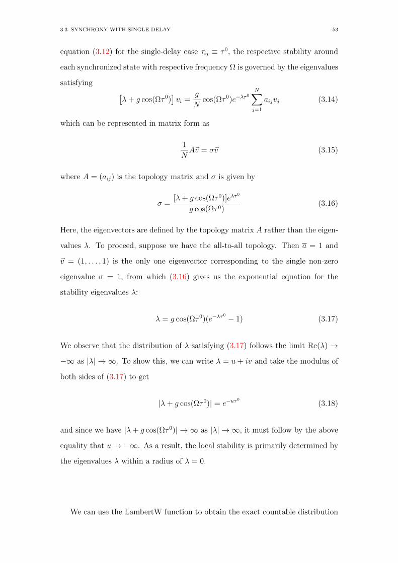
3.3. SYNCHRONY WITH SINGLE DELAY 53
equation (3.12) for the single-delay case τij ≡ τ 0, the respective stability around
each synchronized state with respective frequency Ω is governed by the eigenvalues
satisfying [λ+ g cos(Ωτ 0)
]vi =
g
Ncos(Ωτ 0)e−λτ
0N∑j=1
aijvj (3.14)
which can be represented in matrix form as
1
NA~v = σ~v (3.15)
where A = (aij) is the topology matrix and σ is given by
σ =[λ+ g cos(Ωτ 0)]eλτ
0
g cos(Ωτ 0)(3.16)
Here, the eigenvectors are defined by the topology matrix A rather than the eigen-
values λ. To proceed, suppose we have the all-to-all topology. Then a = 1 and
~v = (1, . . . , 1) is the only one eigenvector corresponding to the single non-zero
eigenvalue σ = 1, from which (3.16) gives us the exponential equation for the
stability eigenvalues λ:
λ = g cos(Ωτ 0)(e−λτ0 − 1) (3.17)
We observe that the distribution of λ satisfying (3.17) follows the limit Re(λ) →
−∞ as |λ| → ∞. To show this, we can write λ = u+ iv and take the modulus of
both sides of (3.17) to get
|λ+ g cos(Ωτ 0)| = e−uτ0
(3.18)
and since we have |λ+ g cos(Ωτ 0)| → ∞ as |λ| → ∞, it must follow by the above
equality that u→ −∞. As a result, the local stability is primarily determined by
the eigenvalues λ within a radius of λ = 0.
We can use the LambertW function to obtain the exact countable distribution

54 CHAPTER 3. KURAMOTO NETWORK MODEL WITH DISTRIBUTED DELAYS
of eigenvalues Λ for (3.17). The eigenvalues λk ∈ Λ, k ∈ Z are given by
λk = −g C0 +Wk(−g C0 exp(g C0τ
0))
τ 0(3.19)
where C0 := cos(Ωτ 0) and Wk(z) is the kth branch of the LambertW function.
Otherwise, we can immediately assess the stability by the following statement1.
Theorem 5. Given the Kuramoto network (3.5) with the all-to-all topology, sup-
pose τij = τ 0 ≥ 0 for all i, j. Then, the system is stable around the in-phase
synchronized state θi(t) = Ωt if and only if g cos(Ωτ 0) > 0, where Ω satisfies
(3.13) for a = 1.
Proof. Let λ = u + iv be any eigenvalue, and suppose u > 0. Then, equating the
real parts of (3.17),
u = g cos(Ωτ 0)[e−uτ0
cos(vτ 0)− 1] (3.20)
from which e−uτ0
cos(vτ 0) < 1. Hence, it must hold that g cos(Ωτ 0) < 0 for the
right-side of the above equation to be positive.
Figure 3.1 shows an instance of the above results with natural frequency ω0 =
1.0 corresponding to a 2π-periodic limit cycle, alongside selected values g = 1.5
and τ 0 = 2.0s. Figure 3.1(A) plots the L-R error (left-hand side minus right-hand
side) of the fixed-point equation (3.13) for the in-phase synchronization frequency
Ω ∈ [ω0 − g, ω0 + g]. We locate three synchronization frequencies Ω1 < Ω2 < Ω3.
Figure 3.1(B) plots the stability criterion cos(Ωiτ0), i = 1, 2, 3 for each synchro-
nization frequency found. With respect to Theorem 5, the synchronized state at
frequency Ωi is stable if cos(Ωiτ0) > 0, and unstable otherwise. We observe that
Ω1 = 0.259, Ω3 = 2.465 are stable and Ω2 = 1.887 is unstable. Figure 3.1(C, D)
plots the exact eigenvalues λk ∈ Λ using the LambertW equation (3.19) at fre-
quencies Ω = Ω1, Ω2 respectively for the initial indexed branches Wk(z), |k| ≤ 10.
We see that the distribution of eigenvalues are consistent with the criterion in The-
1Theorem 5 can be generalized to hold for any connection topology aij . The proof is provided in the mainresult of [17]

3.3. SYNCHRONY WITH SINGLE DELAY 55
orem 5, as there is an eigenvalue with positive real part at the unstable frequency
Ω = Ω2, while all non-zero eigenvalues are on the left-side of the imaginary axis
for stable frequency Ω = Ω1. As a result, the network can synchronize in-phase
with entrained frequency Ω = Ω1 or Ω = Ω3.
Figure 3.1: Theoretical stability plots for the Kuramoto network with single staticdelay. A. The L-H error curve of fixed point equation (3.13) for the in-phase sync. frequencyΩ. There are three sync. frequencies Ω1 < Ω2 < Ω3 on the interval [ω0 − g, ω0 + g]. B. Plotof cos(Ωiτ
0) for each sync. frequency Ωi, i = 1, 2, 3 in reference to plot A. Frequencies whosemarkers are above the x-axis (red line) indicates that the sync. state is stable, and unstableotherwise. C, D, E. Complex scatter plots of the exact stability eigenvalues for frequenciesΩ1, Ω2, Ω3 respectively, using the LambertW equation (3.19) for branch indices k ∈ Z, |k| ≤ 10.With each frequency, the distribution of eigenvalues is consistent with the stability determined bycos(Ωτ0). For all plots, the all-to-all topology aij = 1 is used, and ω0 = 1.0, g = 1.5, τ0 = 2.0s.
We are also interested in how the synchronous frequencies Ω and their respec-
tive stabilities change as the coupling coefficient g and delay τ 0 are increased.
Figure 3.2(A) shows all solution frequencies Ω to (3.13) for each varying g > 0
and fixed delay τ 0 = 2.0s. A bifurcation occurs at some critical coupling strength
gc ≈ 1.42, as two higher synchronization frequencies appear and remain onwards.
Figure 3.2(B) plots the respective stability term cos(Ωτ 0) for each located fre-
quency, where the frequency Ω is stable if cos(Ωτ 0) > 0. There, we see that there
exists a stable lower frequency branch Ω1 < ω0 (blue curve) and a stable higher
frequency branch Ω3 > ω0 (green curve) past the bifurcation value gc. The mid-
dle frequency branch Ω2 (orange curve) remains unstable. Figure 3.2(C) shows

56 CHAPTER 3. KURAMOTO NETWORK MODEL WITH DISTRIBUTED DELAYS
Figure 3.2: Stability plots for the Kuramoto network with increasing coupling andincreasing single delay. A. Plot of all sync. frequencies satisfying (3.13) for varying couplingcoefficient g > 0 and fixed delay τ0 = 2.0s. B. The respective stability criterion plots cos(Ωτ0) ofeach frequency Ω found in plot A. At every g > 0, each frequency’s stability criterion is plottedusing the same colour. C. Plot of all sync. frequencies satisfying (3.13) for varying delay τ0 andfixed coupling g = 0.15. D. The respective stability plot of each frequency Ω found in plot C.For all plots, the all-to-all topology aij = 1 is used, and ω0 = 1.0.
the single solution frequency for each varying delay τ 0 > 0 and fixed small cou-
pling g = 0.15. Here, the synchronization frequency fluctuates around the natural
frequency ω0 = 1.0 as τ 0 increases. Figure 3.2(D) plots the respective stability
criterion for each frequency, where we observe that the synchronous state peri-
odically alternates between stable and unstable as τ 0 increases. Consequently,
for increasing values of τ 0, we are not always ensured a stable synchronization
frequency to exist.
By constraining cos(Ωτ 0) ≤ 0, together with (3.13) we can derive boundary
curves for the stability of the synchronous frequency Ω with respect to parameters
g, τ 0. We have cos(Ωτ 0) ≤ 0 if and only if
(4k + 1)π
2≤ Ωτ 0 ≤ (4k + 3)π
2, k ∈ Z (3.21)

3.4. SYNCHRONY WITH DISTRIBUTED DELAYS 57
from which by the equalities of (3.21) and equation (3.13), it follows that cos(Ωτ 0) =
0 given
(4k + 2± 1)π
2= ω0τ
0 ± gτ 0, k ∈ Z (3.22)
From the two equations above, we obtain the instability region g < g(τ 0), τ 0 > 0,
where g(τ 0) is the parameteric curve
g(τ 0) =
ω0 − (4k+1)π
2τ0, (4k+1)π
2≤ ω0τ
0 ≤ (2k + 1)π, k ∈ Z
(4k+3)π2τ0
− ω0, (2k + 1)π ≤ ω0τ0 ≤ (4k+3)π
2, k ∈ Z
0 otherwise
(3.23)
We reserve discussion of the above derived stability region for later sections.
3.4 Synchrony with distributed delays
We now analyze the synchronous dynamics of the Kuramoto network model (3.5)
with a distribution of connection delays τij > 0. To start off, the single delay
stability criterion around the in-phase synchronous state given in Theorem 5 can
be generalized as follows.
Theorem 6. Given the Kuramoto network (3.5), suppose the delays τij and con-
nection topology aij are such that there exists a frequency Ω such that θi(t) = Ωt
satisfies the self-consistency relation (3.7) with ∆ij ≡ 0. If cos(Ωτij) > 0 for all in-
dices i, j where aij = 1, then the system is stable around the in-phase synchronous
state θi(t) = Ωt.
Proof. The statement is proved using Lyapunov functionals for delay equations in
[55].
While Theorem 6 does provide us with a basic stability region, the criterion
can be seen as too strict as it does not allow for a single delay τij to leave the
region cos(Ωτij) > 0. Indeed, given a large number of oscillators, we can still
expect in-phase synchronization to occur given the vast majority of delays are
within the cosine bound cos(Ωτij) > 0. We seek to define a stability region that

58 CHAPTER 3. KURAMOTO NETWORK MODEL WITH DISTRIBUTED DELAYS
encompasses all distributions of delays that leads to a stable synchronous state. As
part of a statistical approach, it is necessary for us to consider large-N dimensional
networks. For simplicity, we also set the connection topology to be all-to-all (i.e.
aij ≡ 1). Suppose the connection delays τij are i.i.d. sampled from a known
distribution with density ρ(τ). We assume that synchrony must occur in-phase,
for which the common frequency Ω satisfies the fixed-point equation
Ω = ω0 +g
N
N∑j=1
sin(−Ωτij) (3.24)
for each i ≤ N . Taking N → ∞, by the Law of Large Numbers (3.24) can be
approximated as the limit equation
Ω = ω0 + g
∫ ∞0
sin(−Ωτ)ρ(τ) dτ (3.25)
For large-N networks, we can expect the solution Ω to (3.25) to satisfy the self-
consistency equations (3.24) with minimal phase error. By (3.12), local stability
around the in-phase frequency Ω is governed by eigenvalues λ ∈ C, each with
corresponding eigenvector ~v, satisfying the matrix equation
[Dλ − g
Mλ
N
]~v = ~0 (3.26)
where Dλ is a diagonal matrix whose entries are
Dii = λ+g
N
N∑j=1
cos(Ωτij), i ≤ N (3.27)
and Mλ = (Mij) is a random square matrix of i.i.d. entries
Mij = cos(Ωτij)e−λτij , 1 ≤ i, j ≤ N (3.28)
We can forgo consideration of the eigenvector ~v by equating the condition (3.26)
as
det
[Dλ − g
Mλ
N
]= 0 (3.29)

3.4. SYNCHRONY WITH DISTRIBUTED DELAYS 59
Further approximations can be made as follows. Note that as N → ∞, the
diagonal entries Dii → λ + g E[cos(Ωτ)], where E[f(τ)] is the expected value of
f(τij) defined as
E[f(τ)] =
∫ ∞0
f(τ)ρ(τ) dτ (3.30)
and by the Law of Large Numbers, Dλ → (λ + g E[cos(Ωτ)])I, where I is the
identity matrix. By properties of determinants, (3.29) can be approximated by
the equation det[Ψλ,N ] = 0, where Ψλ,N is the matrix defined by
Ψλ,N := I +
(βλN
)Mλ, βλ =
−gλ+ g E[cos(Ωτ)]
(3.31)
Since Mλ is a random matrix, the determinant det[Ψλ,N ] is a random variable.
We choose to express the eigenvalue equation (3.29) in the approximate limit
form (3.31), as the expected value of the determinant can be easily written from
the following theorem.
Theorem 7. Let M be a random N -dimensional square matrix where the entries
Mij are i.i.d sampled such that for all i, j ≤ N , E[Mij] = µ and Var[Mij] = σ2.
Then, for any coefficient β,
E(
det
[I + β
M
N
])= 1 + βµ (3.32)
and the variance has the form
Var
(det
[I + β
M
N
])=
2N∑K=2
(β
N
)K bK/2c∑p=0
αK, p µK−2pσ2p (3.33)
for some coefficients αK, p ∈ Z. In the case where µ = 0, the variance is given by
Var
(det
[I + β
M
N
])=
N∑p=1
(βσ
N
)2pN !
(N − p)!(3.34)
which consist of the terms in (3.33) independent of µ.
Proof. We refer the reader to Appendix B for the proof.
Based on computational simulations, it turns out that determinants of matrices

60 CHAPTER 3. KURAMOTO NETWORK MODEL WITH DISTRIBUTED DELAYS
of the form Ψλ,N satisfies a Central Limit Theorem under certain conditions. We
leave the proof of the following theorem as an open problem, as we will not need to
know the distribution of det[Ψλ,N ] to implement our stability analysis. A similar
statement is given in [51], and such random matrix theorems can potentially have
strong implications in stability theory for large-dimensional systems.
Theorem 8. Let M be a random N -dimensional square matrix where the entries
Mij are i.i.d sampled from a common distribution with density ρ(x) that exponen-
tially decays, such that E[Mij] = µ 6= −1/β for all i, j and the entries Mij have
a sufficiently small variance Var(Mij) = σ2. Then, there exists sequences µN , σN
such thatlog∣∣det
[I + βM
N
]∣∣− µNσN
d−→ N(0, 1) (3.35)
as N →∞ (i.e. converges in distribution to the standard normal distribution).
To apply Theorem 7 to our stability analysis, we approach the eigenvalue cri-
terion (3.31) in a statistical sense. That is, a randomly sampled matrix of de-
lays τ = (τij) ∈ RN×N+ can lead to either stability or instability around the in-
phase synchronous state. Deterministically, the expected distribution of stability
eigenvalues λ ∈ C are given by the equation E(det[Ψλ,N ]) = 0 or equivalently,
E[cos(Ωτ)e−λτ ] = −1/βλ. However, a given sampled distribution of delays τ can
have eigenvalues λ satisfying det[Ψλ,N ] = 0 that deviate widely from the expected
distribution given the variance of delays is large. Therefore, the expected distri-
bution of eigenvalues may not be an accurate descriptor of local stability around
a synchronous state. Nevertheless, we can establish a stability criterion for which
there is strong likelihood of the Kuramoto network being in-phase stable if sat-
isfied. We proceed by fixing an arbitrary real λ > 0. Then, for a given sampled
distribution of delays τ , we can say there is a strong likelihood that there exists
a positive real eigenvalue near λ > 0 if
Var(det[Ψλ,N ]) (E(det[Ψλ,N ]))2 = (1 + βλµλ)2 (3.36)
where Ψλ,N is defined by (3.29), from which det[Ψλ,N ] = 0 is well within one

3.5. SYNCHRONY WITH EXPONENTIALLY DISTRIBUTED DELAYS 61
standard deviation from the mean E(det[Ψλ,N ]). We denote
µλ = E[cos(Ωτ)e−λτ ], σ2λ = Var[cos(Ωτ)e−λτ ] (3.37)
and from the form of the variance (3.33) in Theorem 7, Var(det[Ψλ,N ]) becomes an
increasing function with respect to large σ2λ given µλ fixed, for which Var(det[Ψλ,N ])
is dominated by the positive terms independent of µλ. Therefore, the oscillators
will likely be unstable at the in-phase synchronous frequency Ω if there exists some
real λ > 0 such that σλ is sufficiently large with respect to µλ, indicated by the
inequality (3.36) being satisfied. In the next section, we test the above criterion
in the case of exponentially distributed delays.
3.5 Synchrony with exponentially distributed delays
As an application of the developed theory in the previous section, suppose the
connection delays τij in a large-N all-to-all Kuramoto network are i.i.d. sampled
from the exponential distribution across all indices i, j ≤ N . That is, τij ∼
exp(τm), where τm > 0 is the mean delay. Under the exponential density function
ρ(τ) = µ exp(−µτ), τ > 0, µ = 1/τm (3.38)
the fixed-point equation (3.25) for the synchronization frequency Ω becomes
Ω = ω0 −gµΩ
µ2 + Ω2(3.39)
from which potential synchronization frequencies are given by real roots Ω ∈
[ω0 − g, ω0 + g] of the cubic polynomial equation
Ω3 + ω0Ω2 + (µ2 + gµ)Ω− ω0µ2 = 0 (3.40)
Hence, the Kuramoto model with exponentially distributed delays can have either
zero, one, or three possible synchronous frequencies, depending on the nature of
the roots of (3.40). To analyze the in-phase stability at frequency Ω, we compute

62 CHAPTER 3. KURAMOTO NETWORK MODEL WITH DISTRIBUTED DELAYS
the required mean and second moment
E[cos(Ωτ)e−λτ ] =µ(λ+ µ)
(λ+ µ)2 + Ω2(3.41)
E[cos2(Ωτ)e−2λτ ] =µ
2
(2λ+ µ
4Ω2 + (2λ+ µ)2+
1
2λ+ µ
)(3.42)
By Theorem 7, the expected distribution of the eigenvalues satisfying E(det[Ψλ,N ]) =
0 is given by the roots of the cubic polynomial
λ3 +
(2µ+
gµ2
µ2 + Ω2
)λ2 +
((µ2 + Ω2) +
2gµ3
µ2 + Ω2− gµ
)λ = 0 (3.43)
from which there are two non-trivial eigenvalues.
We simulate the distribution of stability eigenvalues λ around the approximate
in-phase frequency Ω under samples of exponential delays τij as the mean delay
τm increases, while keeping all other parameters fixed. We set the number of
oscillators to be N = 60, alongside large coupling g = 1.5 and natural frequency
ω0 = 1.0. Figure 3.3(A) plots the solution Ω of (3.40) at each mean delay τm,
with step-size ∆τm = 0.5s. All τm within the plotted range resulted in a single
real solution Ω = Ω(τm) as shown, with the two complex solutions ignored. We
observe that Ω < ω0 for all τm as well. This implies that, unlike the single-delay
case τij = τ 0, a varying distribution of delays drives the oscillators to synchronize
at lower frequencies in comparison to their natural frequency. Hence, network
synchrony is easier to achieve at the lower frequency bands, which is needed under
the more difficult scenario of widely distributed connection delays.
For each mean delay τm, Figure 3.3(B) plots the two non-zero expected eigen-
values λ1, λ2 as given by (3.43) at the single synchronous frequency Ω = Ω(τm).
As shown by plotting the real and imaginary parts of each eigenvalue, the eigen-
values remain negative real until some critical mean delay τmc . For τm > τm
c , the
eigenvalues become complex while maintaining negative real parts. Hence, a bi-
furcation occurs at τmc , for which as τm ↑ τm
c , one of the eigenvalues λ1 approaches
0. From this observation τmc can be determined by setting the last coefficient of

3.5. SYNCHRONY WITH EXPONENTIALLY DISTRIBUTED DELAYS 63
Figure 3.3: Stability plots for the Kuramoto network with exponentially sampleddelays. A. Plot of the single sync. frequency Ω satisfying (3.40) with respect to each increasingmean delay τm. B. Plot of the real (magenta) and imaginary (green) parts of the two non-zeroexpected eigenvalues λ1 (x marker), λ2 (square marker) from (3.43) at each τm. C. Plot ofstability criterions with increasing τm at the single sync. frequency as shown in plot A. Thepurple line plots sup Re(Λ) at each τm (purple), where Λ is the set of located eigenvalues nearλ = 0 that satisfy (3.29) with respect to an instance of sampled i.i.d. delays τij ∼ exp(τm).There is a loss of stability as sup Re(Λ) becomes positive near the critical mean delay τm = τmc .The orange line plots − cos(Ωτm). Positive values imply instability around frequency Ω. D,E. Complex plots showing the expected (blue) eigenvalues and actual (red) eigenvalues Λ, inaccordance to a sampled set of exponential delays τij with mean τm = 2.0s, 6.0s and respectivesync. frequency Ω. For all plots, N = 60 with the all-to-all topology aij = 1, and g = 1.5,ω0 = 1.0.
the polynomial (3.43) to 0. That is,
µ4c + gµ3
c + 2µ2cΩ− gµcΩ2 + Ω4 = 0, µc = 1/τm
c (3.44)
By applying cubic root formulas for Ω from (3.40) with (3.44) and numerically
minimizing error, we estimate the critical mean delay to be τmc = 4.94s with
respect to our chosen parameter values. The expected eigenvalues λ1, λ2 imply
that the network under exponential delays remain stable regardless of how large
τm is. By comparing with numerical trials as we will see later on, the expected
eigenvalues are not an accurate descriptor of local synchronous stability of the

64 CHAPTER 3. KURAMOTO NETWORK MODEL WITH DISTRIBUTED DELAYS
network. However, bifurcations regarding eigenvalues λ1, λ2 can be indicative of a
change in network convergence behaviour as we will now see.
We obtain a more direct description of stability as follows. For each mean
delay τm, a matrix of i.i.d. delays τij ∼ exp(τm) was sampled. From this instance
of sampled delays of mean τm, we estimated the locations of the corresponding
distribution of eigenvalues λ satisfying equation (3.29), which we denote as Λ.
This was done by utilizing the fminsearch function in MATLAB. A detailed
explanation about the computational method is given in Appendix D. We denote
sup Re(Λ) as the maximum real component over all non-zero eigenvalues λ ∈ Λ
for each τm. Then, we have a loss of stability if sup Re(Λ) > 0. Figure 3.3(C)
plots sup Re(Λ), from which we note that sup Re(Λ) goes from negative to positive
near τmc . This suggests that τm
c is the bifurcation point at which loss of network
stability occurs. Alternatively, we can treat the sampled delays as a single delay
τij = τm and utilize the single-delay stability condition cos(Ωτm) > 0. Juxtaposing
cos(Ωτm) with sup Re(Λ) > 0 we see that the network operating at single-delay
τm signals a loss of stability at a point sooner than τmc . This implies that the
distribution of the connection delays τij can aid in preserving synchronization
given larger mean delays. Lastly, Figure 3.3(D, E) provides a complex plot of
actual eigenvalues Λ along with the expected eigenvalues λ1, λ2 from (3.43). For
illustrative clarity, we scale the imaginary components of each eigenvalue λ ∈ Λ
using the sign log function
s. log10(x) = sign(x) · log10(1 + |x|) (3.45)
All plotted eigenvalues λ ∈ Λ had a numerical error within log10(det Ψλ,N) < −3.8.
Being consistent with the prior discussion, the eigenvalues for the mean delay
τm = 2.0 < τmc remain on the left side of the imaginary axis, while there exist
some eigenvalues with positive real part for the mean delay τm = 6.0 > τmc .
We provide some more in-depth analysis by computing the standard deviation
of the eigenvalue matrix det[Ψλ,N ]. Figure 3.4(A) compares the mean and standard
deviation µλ, σλ as defined in (3.37) and calculated by exact formulas (3.41, 3.42)

3.5. SYNCHRONY WITH EXPONENTIALLY DISTRIBUTED DELAYS 65
at the arbitrary fixed positive value λ = 0.1. It can be seen that for τm > τmc ,
we have σλ > µλ and this difference increases as τm increases. As discussed in
the prior section, this can lead to det[Ψλ,N ] having a significantly larger standard
deviation than its mean close to λ = 0. We discover a clear difference between the
relation between the mean and standard deviation when we take the limit λ→ 0
while fixing the mean delay τm. Figure 3.4(B, C) plots the mean µλ and standard
deviations σλ while fixing τm = 2.0s, 6.0s respectively and taking λ → 0+. Here,
the limit λ → 0+ is expressed by increasing the term − log10 λ. For τm = 2.0s,
the standard deviation remains smaller than the mean with σλ < µλ as λ → 0+.
For τm = 6.0s, the opposite holds with µλ σλ as λ → 0+. As discussed in the
prior Section 3.4, the limit behaviour µλ σλ as λ → 0+ implies that there is a
large standard deviation of det[Ψλ,N ] near λ = 0+. This is relevant since a large
standard deviation of det[Ψλ,N ] for some small λ > 0 may indicate the existence
of an unstable eigenvalue λ ∈ C satisfying det[Ψλ,N ] = 0 with Re(λ) > 0.
We check whether σλ being large corresponds to a larger det[Ψλ,N ]. We numer-
ically estimate std(det[Ψλ,N ]) at each point λ > 0 and τm by taking the sample
standard deviation of det[Ψλ,N ] numerically computed over 2000 iterations of sam-
pled delays τij ∼ exp(τm), 1 ≤ i, j ≤ N . Figure 3.4(D) compares these estimates
at τm = 2.0s, 6.0s with λ→ 0+. We note that the trend mirrors the results with
µλ, σλ, with std(det[Ψλ,N ]) being significantly large at τm = 6.0s and increasing
as λ→ 0, while std(det[Ψλ,N ]) is small at τm = 2.0s. Overall, there is consistency
between these results and the previous results on the distribution of stability eigen-
values λ ∈ C as shown in Figure 3.3(D, E). That is, higher standard deviations
σλ and std(det[Ψλ,N ]), which occur at larger mean delays τm > τmc , result in a
loss of stability with the existence of positive real eigenvalues. As a nod to the
unproven Theorem 8, we applied the Lillie hypothesis test for normality on each
array of log(det[Ψλ,N ]) and plotted the p-value at each λ → 0+ and mean delays
τm = 2.0s, 6.0s. A small p-value implies rejection of the null hypothesis that
log(det[Ψλ,N ]) is normally distributed. We note that the p-value is fairly large for
both mean delays at λ = 1.0, and then decreases to < 0.001 as λ → 0+. This

66 CHAPTER 3. KURAMOTO NETWORK MODEL WITH DISTRIBUTED DELAYS
Figure 3.4: Expected value and standard deviations of the eigenvalue matrix det[Ψλ,N ].A. Plot of the theoretical mean and standard deviation µλ (blue), σλ (red) from (3.37) withincreasing τm at fixed λ = 0.1. Here, µλ, σλ is normalized by multiplication factor βλ. B, C.Plots of µλ (blue line), σλ (red line) at fixed τm = 2.0s, 6.0s respectively while taking the limitλ→ 0 (or as − log10 λ increases). At τm = 2.0s, the inequality µλ > σλ holds for all small valuesλ near λ = 0+. At τm = 6.0s, the inequality µλ σλ holds and σλ increases as λ → 0+. D.Plot of the (scaled by log10) standard deviation of the eigenvalue matrix Ψλ,N at each decreasingλ → 0+ and fixed τm = 2.0s (purple x), τm = 6.0s (magenta square). E. The p-value of thelillietest for normality of det[Ψλ,N ] at each λ as λ → 0 at τm = 2.0s (green) and τm = 6.0s(black). A small p-value rejects the null hypothesis and implies lack of normality. The values inplots D, E were obtained by taking the sample variance and p-value of det[Ψλ,N ] computed over2000 iterations of sampled delays τij with exponential mean τm. For all plots, N = 60 with theall-to-all topology aij = 1, and g = 1.5, ω0 = 1.0.
implies an overall loss in normality of the random variable log det[Ψλ,N ] as λ→ 0
for both mean delays τm = 2.0, 6.0s. Hence, the lack of normality of log det[Ψλ,N ]
near λ = 0+ is independent of stability. Nevertheless, more work is needed to as-
sess the distribution of log det[Ψλ,N ] at λ and to realize the potential applications
of Theorem 8.
3.6 The incoherent state
A complementary method in analyzing the stability of the Kuramoto model around
the synchronized state is to assess its stability around the incoherent state, which

3.6. THE INCOHERENT STATE 67
represents the oscillatory phases being uniformly distributed on the torus T. In
some cases that we will find, there is an overlap of the stability region boundaries
around the synchronous state and incoherent state. In addition, defining the
distribution of phases with respect to the incoherent state allows us to take a
continuum limit N → ∞ onto the network, which is not as intuitive to do with
the synchronous state. This approach is outlined in [67], with similar results in
[77]. To start, we take the number of oscillators N to infinity. Then, we define the
network of phases to be positioned along the unit circle S in terms of a continuous
density. Let ρ(θ, t) dθ be the fraction of oscillators whose phase lie between θ and
θ+dθ at time t. As a density, the function ρ is non-negative, 2π-periodic in θ and
satisfies the normalization ∫ 2π
0
ρ(θ, t) dθ = 1 (3.46)
To proceed, we assume that the continuum of oscillator phases acts like an in-
compressible fluid. This allows us to say that density ρ(θ, t) is governed by the
Euler-Lagrange equation
dρ
dt= − d
dθ(ρv) (3.47)
where θ is the fluid’s position along the unit circle, and v(θ, t) is the instantaneous
velocity of the fluid at position θ and time t. Likewise to the previous sections,
we assume that the Kuramoto network is all-to-all connected and the connection
delays τij are i.i.d. sampled from the positive density h(τ). Then, we define the
delayed order parameter
ξi(t)eiψi(t) :=
1
N
N∑j=1
eiθj(t−τij) (3.48)
for each i. Taking the imaginary component of (3.48) we can write the Kuramoto
model (3.5) in a mean-field form
θ′i(t) = ω0 + g ξi(t) sin(ψi(t)− θi(t)) (3.49)
Now, by the Law of Large Numbers, taking N →∞ allows us to express (3.48)

68 CHAPTER 3. KURAMOTO NETWORK MODEL WITH DISTRIBUTED DELAYS
as the integrand
ξi(t)eiψi(t) =
∫ 2π
0
∫ ∞0
eiθρ(θ, t− τ)h(τ) dτ dθ (3.50)
Noting that the N -limit is the same for all order parameters, we have ξieiψi ≈ ξeiψ
for all i as N →∞. Hence, the mean-field equation (3.49) as a velocity at phase
position θ and time t can be expressed as
v(θ, t) = ω0 + g ξ(t) sin(ψ(t)− θ) (3.51)
Plugging in (3.51) into (3.47) and expressing the order parameter in its inte-
grand form (3.50) we obtain the single equation for density ρ:
dρ
dt= − d
dθ
[ρ
(ω0 + g
∫ 2π
0
∫ ∞0
sin(θ′ − θ)ρ(θ′, t− τ)h(τ) dτ dθ′)]
(3.52)
which is the Kuramoto model for infinite-dimension N .
To assess the synchronous behaviour of the Kuramoto system in large dimen-
sions, we consider the uniform incoherent state
ρ0(θ, t) =1
2π(3.53)
and determine the stability of the density ρ(θ, t) around ρ0. The incoherent state
ρ0 is the zero solution with respect to global synchrony, as a uniform distribution
of oscillatory phases θ implies the order parameter r = 0. We apply stability
analysis on the state ρ0 by taking the ε-perturbation η(θ, t). Let
ρ(θ, t) = ρ0(θ, t) + εη(θ, t) (3.54)
where ε 1 and the perturbation η can be written as a Fourier series in θ
η(θ, t) = c(t)eiθ + c(t)e−iθ + η⊥(θ, t) (3.55)
where η⊥ are the higher order harmonic terms of η. Due to the sinusoidal coupling
of the Kuramoto model, only the first harmonic, c(t), displays nontrivial dynamics.

3.6. THE INCOHERENT STATE 69
Substituting ρ in (3.54) into (3.52) while ignoring all but the first harmonic c(t)
in (3.55), we get
dc
dt= −iω0c+
g
2
∫ ∞0
c(t− τ)h(τ) dτ (3.56)
Writing c(t) = beλt for any constant b, we wish to evaluate for the eigenvalues
λ ∈ C satisfying the above equation. Plugging in this eigenvalue function we
obtain the equation
λ = −iω0 +g
2Lh(λ) (3.57)
where Lh is the Laplace transform of density h defined as
Lh(λ) =
∫ ∞0
e−λτh(τ) dτ (3.58)
Hence, the stability around the incoherent state ρ0 is determined by the distribu-
tion of eigenvalues λ ∈ C satisfying fixed-point equation (3.57). The incoherent
state is unstable Re(λ) ≥ 0 for some eigenvalue λ, which implies the system pulls
away from incoherence and possibly towards a more coherent asymptotic state.
We consider specific cases of the delay distribution h(τ) and how it affects a
large-N network’s stability around the incoherent state. Given the single delay
case h(τ) = δ(τ − τ 0) for which τij = τ 0 for all i, j, the eigenvalue equation (3.57)
for λ ∈ C is
λ = −iω0 +g e−λτ
0
2(3.59)
We determine the boundary condition at which we have neutral stability around
the incoherent state, which occurs when Re(λ) ≤ 0 for all λ ∈ C satisfying (3.59).
Setting λ = u + iv and equating the real parts of (3.59) we find that u ≤ 0 given
cos(vτ 0) ≤ 0, from which we obtain the bounds
(4k + 1)π
2≤ vτ 0 ≤ (4k + 3)π
2, k ∈ Z (3.60)
where u = 0 when equality holds for either side of (3.60). Now, equating the

70 CHAPTER 3. KURAMOTO NETWORK MODEL WITH DISTRIBUTED DELAYS
imaginary parts of (3.59) and transforming v → −v, we get
v = ω0 −g sin(vτ 0)
2(3.61)
We observe the similarities of (3.60) and (3.61) to (3.21) and (3.13). By identical
steps, the neutral stability region of the incoherent state is given by g < 2 g(τ 0),
τ 0 > 0, where g(τ 0) is the parametric curve defined in (3.23). As a result, the stable
region of the incoherent state contains the unstable region of the synchronous
state. Fixing ω0 = 1.0, Figure 3.5(A) plots the stable region g < 2 g(τ 0) regarding
the incoherent state, as well as the unstable region g < g(τ 0), τ 0 > 0 for the
synchronous state as derived in Section 3.3. By looking at the coloured regions,
we note that the stable incoherent regions periodically appear with increasing
τ 0, with diminishing peak coupling g > 0. This indicates that smaller delays τ 0
generally require stronger coupling in order for the network to avoid the incoherent
regime.
Figure 3.5: Stability plots for the incoherent state of the Kuramoto network. A. Plotof the stability regions instability regions for the incoherent state and the synchronous state ofthe Kuramoto model with respect to single delay τ0 and coupling coefficient g > 0. The red areais the unstable region for the synchronous state θi(t) = Ωt with the red curve g = g(τ0), τ0 > 0as defined by (3.23), while the blue + red region is the neutrally stable region for the incoherentstate with the blue curve g = 2 g(τ0), τ0 > 0. B. Plots of the real part of the two eigenvaluesλ1, λ2 describing the stability around the incoherent state with exponentially distributed delays,scaled by s. log10(x) defined by (3.45). The positive eigenvalue branch Re(λ1) > 0 (red) andnegative eigenvalue branch Re(λ2) < 0 (green) are plotted with increasing mean delay τm. Here,g = 1.5. For both plots, the all-to-all topology aij = 1 is used and ω0 = 1.0.
Now, suppose that the delays τij are distributed in accordance to the exponen-

3.7. NUMERICAL SIMULATIONS FOR SINGLE AND EXPONENTIALLY DISTRIBUTED DELAYS 71
tial distribution h(τ) = µ exp(−µτ) with µ = 1/τm and mean delay τm. Then,
(3.57) becomes the complex quadratic expression
λ2 + (µ+ iω0)λ+ iω0µ−g
2= 0 (3.62)
for eigenvalues λ ∈ C. Hence, the incoherent state under exponentially distributed
delays have two stability eigenvalues λ1, λ2 ∈ C. Fixing the parameters g = 1.5,
ω0 = 1.0, Figure 3.5(B) plots Re(λ1), Re(λ2) as τm increases. For all τm > 0,
we have Re(λ1) > 0 and Re(λ2) < 0 and hence the incoherent state is always
unstable. However, as τm increases, Re(λ1) ↓ 0 while Re(λ2) remains significantly
negative. This result suggests that there is an overall convergence towards neutral
stability for the incoherent state as τm →∞. We note that the eigenvalues fail to
detect the transition from stability to instability of the synchronous state at the
critical point τmc as shown in Section 3.5.
3.7 Numerical simulations for single and exponentially dis-
tributed delays
With numerical simulations, we validate the theoretical analysis committed in the
previous sections to the Kuramoto delay model equipped with single-delay and
exponentially distributed i.i.d. delays. For direct comparison, we fix the same
parameter values as used in the previous figures. Numerical solutions θi(t) with
corresponding derivative solution θ′i(t), i ≤ N for some time interval 0 ≤ t ≤ T to
the Kuramoto model (3.5) were generated by implementing the dde23 function on
MATLAB. To measure levels of synchrony, we rely on the asymptotic estimators
Ω, φi(t), r provided in Section 2.3.
We set the Kuramoto model to a single delay τij = τ 0, and gauge the level of
in-phase synchronization across varying coupling g > 0 and delay τ 0 > 0. We also
set the number of oscillators to be N = 20 with the all-to-all connection topology.
Figure 3.6 shows the frequency and phases of two numerical trials with different
parameter values. Plots with the red-orange colour scheme used parameter values

72 CHAPTER 3. KURAMOTO NETWORK MODEL WITH DISTRIBUTED DELAYS
g = 1.0, τ 0 = 4.0s, while the blue-purple scheme used g = 0.2, τ 0 = 2.5s. Figure
3.6(A, C) shows the instantaneous frequencies θ′i(t) over time. If θ′i(t) → Ω for
some frequency Ω, then this is indicative of entrainment occurring. We see that
in both cases, entrainment occurs. We note that in the red-orange trial, the
oscillators entrain at a higher frequency than their natural frequency ω0 = 1.0,
which was estimated to be Ω = 1.453. Figure 3.6(B, D) shows the phase deviations
φi(t) over time. In both trials, phase-locking occurs with asymptotic convergence
φi(t) → φi for some constant φi ∈ T. However, red-orange trial phase-locks in-
phase, while the synchronization in the blue-purple trial lacks coherence with large
phase deviations. This is reflected in their respective order parameters r(t) shown
in Figure 3.7(E). We can clearly see that r(t) → 1 for the red-orange trial and
r(t)→ 0 for the blue-purple trial.
Figure 3.6: Numerical plots over time for the Kuramoto model with single delay. A,B. Plot of the instantaneous frequencies θ′i(t) and (sine) phase deviations φi(t) over time of atrial with g = 1.0, τ0 = 4.0s. We observe that in-phase synchronization occurs for this trial.C, D. Likewise plots over time of a trial with g = 0.2, τ0 = 2.5s. We observe that entrainmentoccurs, but the synchrony is not in-phase. E. The order parameter of the two trials plotted inA, B (orange) and C, D (blue). Each trial was run up to time T = 300s. The parameters usedwere N = 20 with the all-to-all topology aij = 1, and ω0 = 1.0.
We wish to determine how asymptotic measurements vary in different regions
of parameters g > 0, τ 0 > 0. We proceed by varying g ∈ [0, 1.5], τ 0 ∈ [0, 12] with
step-size ∆g = 0.1, ∆τ 0 = 0.25s. Figure 3.7(A) shows the estimated frequency
Ω for each trial with parameters set at (τ 0, g). We note that as τ 0 increases, the
estimated synchronization frequency Ω fluctuates between the natural frequency
ω0 = 1.0. Specifically, Ω alternates between regions of Ω > ω0 (indicated by

3.7. NUMERICAL SIMULATIONS FOR SINGLE AND EXPONENTIALLY DISTRIBUTED DELAYS 73
green) and Ω < ω0 (indicated by purple). This mirrors the trend displayed in
Figure 3.2(C) for the theoretical synchronous frequencies Ω, where similar fluctu-
ations are seen under fixed coupling g and increasing τ 0. Figure 3.7(B) shows the
respective asymptotic order r for each trial.
We assess whether stability criterions established in prior sections align with
the numerical results by plotting the neutral stability curves g = g(τ 0) (red) for
the synchronous state and g = 2 g(τ 0) (yellow) for the incoherent state, where g is
defined by (3.23). We observe that the points (τ 0, g) where r ≈ 0 (lack of coherent
synchrony) are contained in the neutral stable region of the incoherent state.
However, some of these points (τ 0, g) also lie inside of the stable region for the
synchronous state. This implies that synchrony can occur with stable incoherence,
as it shows the criterion cos(Ωτ 0) ≥ 0 does not capture the existence of large
constant phase perturbations onto the in-phase synchronous state θi(t) = Ωt. All
solutions for the numerics with single delay were generated up to time T = 300s,
and all estimates were obtained by applying the asymptotic estimates by averaging
along the endtime interval h = 0.1T .
Figure 3.7: Numerical plots for asymptotic values of the Kuramoto model with singledelay. A. Heatmap of the asymptotic sync. frequencies Ω of different trials with parametersg ∈ [0, 1.5], τ0 ∈ [0, 12]. The parameters varied with step-sizes ∆g = 0.1, ∆τ0 = 0.25. Here,
green indicates that Ω > ω0 = 1.0, and purple indicates Ω < ω0. B. Heatmap of the asymptoticorder r of the same trials plotted in A. The neutral stability curves g = 2 g(τ0) for the incoherentstate (yellow) and g = g(τ0) for the synchronous state (red) are also shown. Each trial was runup to t = 300s. The parameters used were N = 20 with the all-to-all topology aij = 1, andω0 = 1.0.
Now we simulate the Kuramoto model with exponential i.i.d. sampled con-

74 CHAPTER 3. KURAMOTO NETWORK MODEL WITH DISTRIBUTED DELAYS
nection delays τij exp(τm) with mean delay τm. Here, we increase the number of
oscillators to large N = 60, and fix the coupling to g = 1.5. Likewise to the single-
delay case, Figure 3.8 shows the frequency and phases of two numerical trials with
different parameter values. Plots with the red-orange colour scheme pertains to
the solution with mean delay τm = 2.0, while the blue-purple scheme has mean
delay τm = 6.0. Figure 3.8(A, C) shows the instantaneous frequencies θ′i(t) over
time, from which we see that entrainment occurs at τm = 2.0s and fails at higher
mean delay τm = 6.0s. Similarly results show with the phase deviations plotted in
figure 3.8(B, D). Phase-locking occurs with minimal phase deviations at τm = 2.0,
while the phases remain incoherent at τm = 6.0s. Figure 3.8(E) shows the density
of sampled connection delays τij used to generate the solutions in the prior plots.
With a larger mean delay τm = 6.0s, there are a greater number of large delays
τij > τm in comparison to τm = 2.0s as the standard deviation of the exponential
distribution is equal to its mean. Figure 3.8(F) shows the corresponding order
parameter r(t) over time for each solution. As consistent with the prior observa-
tions, r(t)→ 1 for τm = 2.0 as t→∞ for τm = 2.0s, while r(t) hovers near 0 for
τm = 6.0s.
Figure 3.8: Numerical plots of over time for the Kuramoto model with exponentiallydistributed delays. A, B. Plot of the instantaneous frequencies θ′i(t) and (sine) phase devia-
tions φi(t) over time of a trial with τm = 2.0s. We observe that in-phase synchronization occursfor this trial with small phase-locked deviation. C, D. Likewise plots over time of a trial withτm = 6.0s. Neither entrainment of frequencies nor phase-locking occurs. E. Histogram of theexponentially sampled delays τij for the two trials plotted in A, B (orange) and C, D (blue). F.The order parameter of the two trials plotted with the same colour scheme. Each trial was runup to time T = 500s (displayed up to 100s here). The parameters used were N = 60 with theall-to-all topology aij = 1, and g = 1.5, ω0 = 1.0.

3.7. NUMERICAL SIMULATIONS FOR SINGLE AND EXPONENTIALLY DISTRIBUTED DELAYS 75
Figure 3.9 explores the effect of increasing τm to asymptotic values of solu-
tions. The mean delay is increased with step-size ∆τm = 0.5s, and we measure
the convergence values of the generated solution θi(t), θ′i(t) with sampled delays τij
having mean τm. In figure 3.9(A), the N -limit theoretical frequency Ω from (3.40)
is plotted alongside the estimated frequency Ω. The two frequencies Ω, Ω closely
align until the solutions θ(t) numerically lose their asymptotic synchrony. Fig-
ure 3.9(B) plots sup Re(Λ), defined as the largest real part of non-zero eigenvalues
λ ∈ Λ satisfying det[Ψλ,N ] = 0 for the sampled delays τij at each mean τm. This
is the same stability plot as in Figure 3.3(C). We determine whether this aligns
with the numerical loss of stability. Figure 3.9(C) plots the asymptotic order r for
each solution used in the frequency plot figure 3.9(A). We observe a sudden drop
in r at τm = 4.5s, which is close to where the sup Re(Λ) → 0. Hence, the loss
of synchrony is dependent on sup Re(Λ), from which there is merit in predicting
the bifurcation point of sup Re(Λ) by comparing the mean and variances of the
stability matrix variables. All solutions for the numerics with single delay were
generated up to time T = 500s, and all estimates were obtained with h = 0.1T .
Figure 3.9: Numerical plots for asymptotic values of the Kuramoto model with ex-ponentially distributed delays. A. Plots of the estimated frequency Ω (black) from solutionθ′i(t) with sampled delays τij ∼ exp(τm) at each τm, and the corresponding theoretical frequencyΩ (magenta) using equation (3.40). The frequencies align closely until τm ≈ 4.0s, at which thesynchronous state begins to lose its stability. B. Plot of the largest real part sup Re(Λ) acrossall non-zero eigenvalues λ such that det[Ψλ,N ] = 0 for each mean delay τm. The matrix Ψλ,N
is defined by (3.31) from a a sample of delays τij ∼ exp(τm). C. The asymptotic order r for asolution θi(t) with sampled delays τij ∼ exp(τm). For each τm, the same trial was used across allplots. The mean delay is varied with step-size ∆τm = 0.5s. The parameters used were N = 60with the all-to-all topology aij = 1, and g = 1.5, ω0 = 1.0.

76 CHAPTER 3. KURAMOTO NETWORK MODEL WITH DISTRIBUTED DELAYS
3.8 Summary
We conclude from these findings that the Kuramoto model with static connection
delays τij faces difficulties in achieving synchronization, which can be portrayed
through both numerically generated phase solutions θi(t) and our theoretical sta-
bility analysis. As shown by looking at the case of single-delay and exponentially
distributed delays, there is a general loss in the oscillators’ ability to synchronize
with larger connection delays with higher variance. This suggests some adaptation
is required at a temporal level to ensure phase synchronization occurs, particu-
larly when the delays are distance-based with axonal connections among a neural
population. We see how this can be accomplished in the upcoming section, where
we implement a phenomenological plasticity rule on the delays.

Chapter 4
Kuramoto model with adaptive
delays
In this section, we now approach the synchronization problem in Kuramoto models
with adaptive delays, and compare the results with the non-adaptive delays as
done in the previous chapter. Adaptive delays may provide a way to acquire
a distribution of delays that is optimal for phase synchronization of Kuramoto
oscillators. Enabled with adaptive delays, our model corresponds to an N + N2
dimensional functional differential equation with state-dependent delays. That is,
N oscillator phases θi(t) and N2 connection delays τij(t). The analysis of such
systems with state-dependent delays is technically challenging [25, 76, 14], and
so we assess the effects of allowing our delays to adapt in accordance to a basic
plasticity rule. This chapter in its entirety has been published [56] as the journal
‘Synchronization and resilience in the Kuramoto white matter network model with
adaptive state-dependent delays’ by the Journal of Mathematical Neuroscience
(2020).
4.1 Modeling adaptive delays
Likewise to Chapter 3, we consider a network of N weakly-coupled non-linear and
delayed Kuramoto oscillators whose phases θi(t) evolve in accordance to (3.5).
However, in this scenario we assume the transmission delays τij = τij(t) fluctuate
77

78 CHAPTER 4. KURAMOTO MODEL WITH ADAPTIVE DELAYS
in time. Recall from Section 1.5 that the transmission delay τij is the sum of
the conduction delay τCij affected by axonal myelination and the synaptic delay
τBij . Since we want to emphasize the effects of conduction delays, we assume that
the synaptic delay is negligible by setting τBij ≈ 0 for all i, j, from which the
conduction delay τCij is equal to the transmission delay τij. The axonal conduction
delays τCij correspond to the conduction time taken by an action potential along
a myelinated fiber. The propagation speed cij = cij(t, `) fluctuates with respect
to a signal’s position ` along the length of an axon as saltatory conduction occurs
at successive nodes of Ranvier. As a consequence of ongoing myelination along
the axonal segments, the instantaneous conduction velocity cij(t, `) at position `
changes slowly in time t. From this, each conduction delay may be expressed as
τij(t) =
∫Pij
c−1ij (t, `) d`, 1 ≤ i, j ≤ N (4.1)
That is, a line integral along the axonal pathway Pij connecting oscillator j to
i. It is uncertain how neural activity and/or oscillatory brain dynamics influ-
ences myelin formation. However, this detailed plasticity relation is difficult to
formulate, and requires precise data on myelination patterns in order to properly
integrate into the model. Our goal is to tentatively observe the types of temporal
dynamics that can arise from adaptive mechanisms. As a prototypical approach,
we consider the Kuramoto model
dθidt
= ω0 +g
N
N∑j=1
aij sin(θj(t− τij(t))− θi(t)), i ≤ N (4.2)
where the delays τij(t) follow the simple sublinear plasticity rule
α−1τ
d
dtτij(t) = H(τij(t)) ·
[−(τij(t)− τ 0
ij) + κ · sin(θj(t)− θi(t))]
(4.3)
where 1 ≤ i, j ≤ N . Here, ατ ≤ 1 is the homeostatic rate constant that sets the
time scale of the evolving delays, which must be slow as discussed in Section 2.5.
The plasticity coefficient κ > 0 sets the gain of the conduction delay changes. The
initial condition for delays τij(t) at t = 0 is provided by baseline lags τ 0ij ≥ 0. That

4.2. SYNCHRONIZED STATE AND STABILITY WITH PLASTIC DELAYS 79
is, τij(0) = τ 0ij for all i, j. The Heaviside function H(τ) is defined as a smooth
function such that H(τ) = 0 if τ < 0 and H(τ) = 1 if τ > ε for some small ε > 0.
The Heaviside function H(τ) is present to preserve the non-negativity of the delays
τij(t) at all times t ≥ 0. For details on the construction of the smooth Heaviside
function, we refer the reader to Appendix C. According to this rule, fluctuations
in conduction delays are governed by an interplay between a local drift component
that represents metabolic inertia towards an initial baseline lag τ 0ij representing
minimal myelination, and a forcing term that depends on the phase difference
∆ij := θj − θi between oscillators i and j.
A schematic of the network structure as well as the activity-dependent plasticity
rule are plotted in Figure 4.1. There, given |θj−θi| < π, one can see that whenever
θj > θi, the time delay increases due to an effective reduction in conduction velocity
caused by myelin retraction. The opposite occurs if θj < θi and the time delay
decreases: the connection speeds up due to myelin stabilization [16]. If the phase
is the same, no changes in conduction velocity are required, and the delay remains
stable at its initial lag τ 0ij.
Under the plasticity rule (4.3), new issues regarding the existence and unique-
ness of solutions becomes an issue. This is not an issue as long as all relevant
functions are sufficiently smooth, as stated by the following theorem.
Theorem 9. The Kuramoto model (4.2) with adaptive delays τij = τij(t) following
the plasticity rule (4.3) has a unique solution θi(t), τij(t), i, j ≤ N given that the
history function ϕi : [−r, 0]→ T for θi(t) is smooth at all times. Furthermore, the
existing delay solutions τij(t) are bounded.
Proof. We refer the reader to Appendix B for the proof of this statement.
4.2 Synchronized state and stability with plastic delays
Mathematically, we analyze the network’s ability (4.2) to asymptotically achieve
the synchronized state θi(t) = Ωt+φi for some global frequency Ω and small phase
deviations φi as t → ∞. Applying the synchronous state ansatz (3.6) onto both

80 CHAPTER 4. KURAMOTO MODEL WITH ADAPTIVE DELAYS
Figure 4.1: Schematic of a network of coupled oscillators with plastic conductiondelays implementing temporal control of global synchronization. The network is builtof recurrently connected phase oscillators, and connections are subjected to conduction delays.Those delays are regulated by a phase-dependent plasticity rule. Depending on whether the phasedifference between two oscillators is positive, zero, or negative, the delays are either increased(myelin retraction), unaltered, or decreased (stabilization).
the phases (3.5) and the delays as in (4.3) , we obtain the expressions for the
global frequency Ω ∈ R and individual offsets φ = (φ1, . . . , φN) ∈ RN as
Ω = ω0 +g
N
N∑j=1
aij sin(−ΩτEij + ∆ij) (4.4)
τEij = max(τ 0ij + κ sin(∆ij), 0) (4.5)
for all i, j, where ∆ij = φj − φi. The above equations (4.4, 4.5) replace the self-
consistency criterion for the global frequency Ω and phase-locked deviations φi. It
must hold that if Ω satisfies (4.4), then Ω ∈ [ω0−g, ω0+g]. To assess the network’s
stability at the synchronized state (Ω,φ) satisfying (3.6, 4.5), we introduce the
perturbation terms εi(t), ηij(t) around the equilibrium states (4.4) and (4.5) for

4.2. SYNCHRONIZED STATE AND STABILITY WITH PLASTIC DELAYS 81
θi(t) and τij(t) respectively. That is, we write
θi(t) = Ωt+ φi + εi(t) (4.6)
τij(t) = τEij + ηij(t) (4.7)
and examine the stability at the equilibrium point εi(t) = ηij(t) = 0. The delay
perturbations ηij(t) abide by the linearized form of (4.3) around all positive delays
τEij = τ 0ij + κ sin(∆ij) > 0. For the equilibrium delays τEij = 0, we proceed by
assuming the corresponding perturbation terms will act in an asymptotically stable
manner. Specifically, for all phase offset differences such that τEij = 0, by the
nature of the Heaviside cutoff function H(τ) in (4.3) there exists some tasy ∈ R
such that for all t > tasy, τij(t) = 0 and consequently ηij(t) = 0. That is, if
τEij = 0, the perturbation term is asymptotically ηij(t) = 0. This condition will
be satisfied given the synchronous state (Ω,φ) is indeed stable. Since the purpose
of linearization is to determine stability, the above assumption is valid to make
before proceeding. Taken together, the linearized equations for the terms ηij(t) as
τij(t)→ τEij are given by
d
dtηij(t) =
−ηij(t) + κC0
ij(εj(t)− εi(t)) if τEij > 0
0 if τEij = 0
(4.8)
where C0ij := cos(∆ij). Inserting (4.6) and (4.7) into the Kuramoto model (4.2),
d
dtεi(t) = ω0−Ω+
g
N
N∑j=1
aij sin(−Ω(τEij +H(τEij )ηij(t)) + ∆ij + εj(t− τEij )− εi(t)
)(4.9)
where we have made the approximation εj(t − τij(t)) ≈ εj(t − τEij ) when τij(t)
is near τEij . With (Ω,φ) satisfying (4.6), and by taking a first-order expansion
around the term −ΩτEij , we obtain the linear system for the phase perturbation
term given by
d
dtεi(t) =
g
N
N∑j=1
aijCij[εj(t− τEij )− εi(t)− ΩHijηij(t)] (4.10)

82 CHAPTER 4. KURAMOTO MODEL WITH ADAPTIVE DELAYS
where we denote Cij = cos(−ΩτEij + ∆ij) and Hij = H(τEij ). Hence, the network
synchronizes at (Ω,φ) given that all perturbation terms εi(t), ηij(t) following the
linear system of fixed delay differential equations (4.8, 4.9) converges to 0. From
here, we can analyze the stability at the synchronous point (Ω,φ) by setting the
ansatz εi(t) = vieλt, ηij(t) = wije
λt with respect to eigenvalue λ ∈ C. By (4.8),
the coefficients wij satisfy
wij = κC0ijHij
(vj − viλ+ 1
)(4.11)
for all i, j, λ 6= −1. Applying (4.11) to coefficients wij,
λvi =g
N
N∑j=1
aijCij
[vje−λτEij − vi − ΩκC0
ijHij
(vj − viλ+ 1
)](4.12)
That is, λ is an eigenvalue if there exists an eigenvector ~v = (v1, . . . , vN) ∈ CN
satisfying (4.12). In matrix form, (4.12) can be expressed as
[Dλ −
gMλ
N
]~v = ~0 (4.13)
where D, M are N -dimensional square matrices defined as follows. D is the
diagonal matrix with diagonal entries
Dii = λ(λ+ 1) +g
N
N∑j=1
aijCij(λ+ 1− ΩκC0ijHij), 1 ≤ i ≤ N (4.14)
and Mλ has entries
Mij = aijCij
[(λ+ 1)e−λτ
Eij − ΩκC0
ijHij
], 1 ≤ i, j ≤ N (4.15)
In summary, we acquire the following stability criterion: The system is (neutrally)
stable around the synchronized state (Ω,φ) if Re(λ) ≤ 0 for all eigenvalues λ ∈ C
satisfying det[Ψλ,N ] = 0, where Ψλ,N is the N ×N matrix given by
Ψλ,N := Dλ −( gN
)Mλ (4.16)

4.3. SYNCHRONIZATION OF TWO COUPLED OSCILLATORS WITH PLASTIC DELAYS 83
Of note is that our approach is an extension of the non-plastic case. Indeed,
without plasticity κ = 0, the delays remain fixed at the baseline lag τ 0ij, and as
a result there is no need for the delays to establish an equilibrium with positive
phase offset differences ∆ij. Hence, the oscillators become perfectly in-phase with
φi = 0 during synchronization, from which the matrices Dλ, Mλ defined by (4.14),
(4.15) are given by (3.27), (3.28) respectively and we obtain the stability criterion
given in Section 3.4.
4.3 Synchronization of two coupled oscillators with plastic
delays
As a first illustrative approach to the general case when the number of coupled
oscillators is large, we consider a reduced two-oscillator network. The following
setup is similar to the system analyzed in [4]. We let N = 2 with a12 = a21 = 1
and remove all self-integration terms by setting a11 = a22 = 0. We also set the
baseline delays to be equal with τ 012 = τ 0
21 = τ 0. Then, the phases θ1(t), θ2(t) follow
the Kuramoto system
θ′1(t) = ω0 + g sin(θ2(t− τ12(t))− θ1(t))
θ′2(t) = ω0 + g sin(θ1(t− τ21(t))− θ2(t))(4.17)
with respective plasticity equations
τ ′12(t) = H(τ12(t)) · [−(τ12(t)− τ 0) + κ sin(θ2(t)− θ1(t))]
τ ′21(t) = H(τ21(t)) · [−(τ21(t)− τ 0)− κ sin(θ2(t)− θ1(t))](4.18)
By symmetry we may let ∆12 = φ2 − φ1 > 0. We proceed by setting a sufficiently
large plasticity gain with κ τ 0. Then, it follows that the respective equilib-
rium delays are τE12 := τ 0 + κ sin(∆12) and τE21 = 0, resulting in a single positive

84 CHAPTER 4. KURAMOTO MODEL WITH ADAPTIVE DELAYS
equilibrium delay. Hence, by (4.4) the frequency Ω and offset ∆12 satisfies
Ω = ω0 + g sin(−ΩτE12 + ∆12) (4.19)
Ω = ω0 − g sin(∆12) (4.20)
Solving for ∆12 above, we obtain
∆12 = arcsin
(ω0 − Ω
g
)> 0 (4.21)
where positivity holds only when Ω < ω0. This leads to the oscillators synchroniz-
ing at a lower frequency Ω ∈ [ω0 − g, ω0). Substituting ∆12 in (4.19) with (4.21),
the synchronous frequency Ω is given by the fixed-point equation
Ω = ω0 + g sin
(−Ω
(τ 0 + κ
(ω0 − Ω
g
))+ arcsin
(ω0 − Ω
g
))(4.22)
Then, θ1(t), θ2(t) synchronizes at a common frequency Ω implicitly satisfying
(4.22). Since it was assumed that τE21 = 0, for self-consistency the synchronous
frequency Ω must also satisfy τ 0 − κ sin(∆12) < 0, which can be written as
Ω < ω0 − gκ−1τ 0 ≈ ω0 since we set κ τ 0. Without plasticity κ = 0, the
oscillators become in-phase with ∆12 = 0 and synchronizes at a frequency Ω given
by the single-delay equation (3.13).
Setting the parameter values to be g = 1.5, ω0 = 1.0, Figure 4.2(A) plots
the L-R error (left-hand side minus right-hand side) of (4.22) on the interval
[ω0−g, ω0) with respect to representative values κ = 0, 20, 30 of the plasticity gain.
Here, we denote the L-R error at Ω as Rκ(Ω). We observe that higher plasticity
gains κ > 0 generally leads to a greater number of potential synchronization
frequencies Ω smaller than the natural frequency ω0 for our system. We can see
that R0(Ω), R20(Ω) have single roots within the interval [ω0−g, ω0) for κ = 0, 20,
while R30(Ω) has five roots within the interval [ω0 − g, ω0).
As derived in Section 4.2, the stability of the oscillators at the synchronization
state (Ω,∆12) is determined by the distribution of eigenvalues λ ∈ C that satisfy

4.3. SYNCHRONIZATION OF TWO COUPLED OSCILLATORS WITH PLASTIC DELAYS 85
Figure 4.2: Stability plots for the 2-dim Kuramoto network with adaptive delay. A.Plot of the L-R error functions Rκ(Ω) with varying fixed gain κ = 0 (magenta), κ = 20 (yellow),and κ = 30 (blue). All roots Ω < ω0 of Rκ(Ω) are potential synchronization frequencies forthe two oscillator system. The number of roots Ω increase with larger κ. B. Plot of the largestreal part among non-zero stability eigenvalues, denoted sup Re(Λ; Ω), at each sync. frequencyΩ given by the roots of Rκ(Ω) at κ = 30. C, D. Complex plots of stability eigenvalues aroundfrequencies Ω = Ω3, Ω4 respectively, where Ω1 < Ω2 < · · · < Ω5 < ω0 are the five sync.frequencies at κ = 30. The parameters used are g = 1.5, ω0 = 1.0 , τ0 = 2.0s.
(4.16). In the 2-dimensional case, we have
det
∣∣∣∣∣∣λ(λ+ 1) + C12(λ+ 1− ΩκC0) −C12(e−λτE12(λ+ 1)− ΩκC0)
−C21 λ+ C21
∣∣∣∣∣∣ = 0 (4.23)
where C12 = g cos(−ΩτE12 + ∆12), C21 = g cos(∆12), C0 = cos(∆12). This results
in the root equation PΩ(λ) + QΩ(λ)e−λτ = 0, where τ = τE12 is the single positive
equilibrium delay and PΩ(λ), QΩ(λ) are polynomials given by
PΩ(λ) = λ3 + (1 + C12 + C21)λ2 + [κC12 + (1 + C12)C21]λ+ C12C21 (4.24)
QΩ(λ) = −C12C21(λ+ 1) (4.25)
where κ = 1−ΩκC0. Note that PΩ(0) +QΩ(0) = 0, which means we have neutral

86 CHAPTER 4. KURAMOTO MODEL WITH ADAPTIVE DELAYS
stability.
For each synchronization frequency Ω that satisfies (4.22) at large gain κ = 30,
the corresponding stability eigenvalues λ ∈ C given by (4.23) near 0 was located
numerically using an fminsearch in MATLAB. We denote sup Re(Λ; Ω) to be the
largest real part among the set of located non-zero eigenvalues Λ for frequency Ω.
If sup Re(Λ; Ω) < 0, then by our stability criterion, the frequency Ω defines a stable
synchronous state. Otherwise, it is unstable. Figure 4.2(B) plots sup Re(Λ; Ω) at
each of the five synchronization frequencies Ω1 < Ω2 < · · · < Ω5 < ω0, from which
we find that Ω3 = 0.725, Ω5 = 0.969 are stable frequencies while the rest are unsta-
ble. Figures 4.2(C,D) shows the complex plot of the located eigenvalues for stable
frequency Ω = Ω3 and unstable frequency Ω = Ω4 respectively. The distribution
of the plotted eigenvalues illustrate the stable and unstable frequencies Ω3, Ω4
respectively, with a significantly positive real eigenvalue appearing for Ω = Ω4.
These results in the simplified two-oscillator case highlight that under sufficiently
large plasticity gain, adaptive delays introduce multiple low-frequency stable states
(Ω,∆12). We compare this result to the single-delay results in Chapter 3. With a
non-adaptive single delay, there exists at most one stable synchronous frequency
Ω < ω0 across different couplings g > 0 and delays τ 0. This suggests that an
adaptive regime leads the Kuramoto oscillators to be able to synchronize at a
greater number of frequencies. In addition, adaptive delays cause the oscillators
to synchronize at lower frequencies relative to their uncoupled natural frequency
ω0.
4.4 Synchronization in large-scale oscillator networks with
plastic delays
Now suppose we have a large N -dimensional system (4.2) with the all-to-all topol-
ogy aij ≡ 1. Again for simplicity, we set the baseline lags to be constant with
τ 0ij ≡ τ 0. The main difficulty in assessing the synchrony of large-dimensional
systems is the uncertainty revolving around the synchronization state (Ω,φ) sat-

4.4. SYNCHRONIZATION IN LARGE-SCALE OSCILLATOR NETWORKS WITH PLASTIC DELAYS 87
isfying the self-consistency equation (4.4). As discussed in Section 3.2, while it is
likely that a synchronous state θi(t) = Ωt + φi exists, it is difficult to determine
how the system will synchronize when the synchrony is not expected to be in-
phase. Unlike our simple 2-dimensional case in Section 4.3, in large-dimensional
systems there can exist several possible frequencies and phase deviations φ sat-
isfying the self-consistency equation. Rather than trying to find exact solutions,
we approach the synchronization state (Ω,φ) in the following statistical sense.
Suppose that under synchrony, the phase-locked deviations φi follow some distri-
bution with standard deviation δ. We can set the φi’s to be centered at 0 by
shifting φi → φi − φ, where φ is the mean of each φi. As an approximation, we
write that the phase differences ∆ij := φj − φi are i.i.d. under some common
density ρ(∆) across all indices i, j. Since ∆ij = −∆ji, the density satisfies the
symmetry ρ(∆) = ρ(−∆) as well. In addition, the differences ∆ij have approxi-
mate standard deviation√
2δ. Now, averaging the self-consistency equation (4.4)
over all indices i and taking the limit N → ∞, we obtain the following N -limit
approximation for the synchronization frequency Ω:
Ω = ω0 + g
∫ ∞−∞
sin(−ΩτE(∆) + ∆)ρ(∆) d∆ (4.26)
where τE(∆) = H(τ 0 +κ sin ∆) ·(τ 0 +κ sin(∆)). In order to apply (4.26) to obtain
the global frequencies Ω, we parametrize the unknown density ρ(∆) by assuming
it is Gaussian with some small variance 2δ2. That is, we set ρ(∆) = ρδ(∆) such
that
ρδ(∆) =1√
4πδ2exp
(−∆2
4δ2
)(4.27)
Without plasticity, we have in-phase synchronization ∆ij = 0 from which ρδ(∆)
is the dirac delta distribution at 0 and (4.26) becomes
Ω = ω0 + g sin(−Ωτ 0) (4.28)
which agrees with (3.13) for a single static delay τij(t) = τ 0. Figure 4.3(A) plots
the L-R error R(Ω, δ2) for (4.26) for various fixed values of δ2 > 0 on interval

88 CHAPTER 4. KURAMOTO MODEL WITH ADAPTIVE DELAYS
Ω ∈ [0, ω0 + g]. We keep the other parameter values consistent with Section 4.2 at
g = 1.5, ω0 = 1.0, τ 0 = 0.1s. We find that there is a unique root Ω toR(Ω, δ2) = 0
at each fixed variance δ2 > 0. Hence, we can obtain an implicit curve Ω = Ω(δ)
to (4.26) with respect to δ > 0. The curve Ω = Ω(δ) is plotted in Figure 4.3(B)
with step-size ∆δ = 0.05 on interval [0, 0.10], and shows a continuous range of
potential synchronization states (Ω(δ), δ) along δ > 0 to a large N -dimensional
system of oscillators. The graph of curve Ω = Ω(δ) also shows that Ω(δ) < ω0 for
all δ > 0, once again implying that the oscillators are drawn to synchronize at a
lower frequency from their natural frequency.
Figure 4.3: Theoretical synchronization frequencies for a large N-dim oscillator sys-tem A. Plots of the L-R error function R(Ω, δ2) of (4.26), with varying fixed δ > 0 overΩ ∈ [0, ω0 + g]. There is a unique sync. frequency Ω = Ω(δ) for each fixed δ > 0. B. Plotof the frequency Ω = Ω(δ) over increasing δ > 0. The parameters used are g = 1.5, ω0 = 1.0,κ = 80, and τ0 = 0.1s.
For small phase differences ∆ij, the equilibrium delays are approximately τEij ≈
τ 0 + κ∆ij if ∆ij > 0 and τEij = 0 if ∆ij < 0. Before proceeding, we set κ to
be sufficiently larger than the baseline lag τ 0 such that τ0
κ≈ 0. Then, most
negative differences ∆ij < 0 fall below the Heaviside cutoff τ 0 + κ∆ij < 0. From
this, the Heaviside term becomes approximately dependent on the sign of ∆ij
with Hij ≈ H(∆ij) for all i, j. For large gain κ, two categories of equilibirum
delays emerge that contribute to the global frequency Ω in (4.26): For half the
connections with phase difference ∆ij < 0, the corresponding delays τij(t) decay
to τEij = 0 as we have τ 0 < −κ∆ij < 0 with τ 0 κ. Otherwise, with ∆ij > 0

4.4. SYNCHRONIZATION IN LARGE-SCALE OSCILLATOR NETWORKS WITH PLASTIC DELAYS 89
the delay τij(t) establishes a positive equilibrium at τEij = τ 0 + κ∆ij. The positive
delays τEij become widely distributed with a large standard deviation of κ√
2δ.
The coupled network can synchronize towards any stable point (Ω, δ) along the
curve Ω = Ω(δ), δ > 0. To assess the stability at each state (Ω, δ), we consider the
N -dimensional eigenvalue criterion (4.16) for λ ∈ C. Under the assumption that
the phase differences ∆ij are i.i.d. with ∆ij ∼ N(0, 2δ2), det[Ψλ,N ] follows some
random distribution. Since the computation of det Ψλ,N requires exact values
of ∆ij, we choose to focus on computing the expected eigenvalues λ satisfying
E(det[Ψλ,N ]) = 0. We start by fixing (Ω, δ) and setting κ τ 0. Note that as
N →∞, the entries Dii for the diagonal matrix Dλ defined by (4.14) converge to
the expected value µλ,D given by
µλ,D := λ(λ+ 1) + g
∫ ∞−∞
CΩ(∆)[λ+ 1− Ωκ cos(∆)H(∆)]ρδ(∆) d∆ (4.29)
by the Law of Large Numbers, where CΩ(∆) = cos(−ΩτE(∆)+∆). Here, we used
the approximation H(τE(∆)) ≈ H(∆), which is justified by the above discussion.
Hence, for large N the condition det[Ψλ,N ] = 0 is equivalent to
det
[I +
βλMλ
N
]= 0, β = −g/µλ,D (4.30)
Furthermore, each entry Mij in the matrix Mλ defined in (4.15) has expected value
µλ,M given by
µλ,M :=
∫ ∞−∞
C(∆)[(λ+ 1)e−λτ
E(∆) − Ωκ cos(∆)H(∆)]ρ(∆) d∆ (4.31)
where τE(∆) ≈ H(∆) · (τ 0 + κ∆). By Theorem 7, the above determinant (4.30)
has expectation
E(
det
[I +
βλMλ
N
])= 1− g
(µλ,Mµλ,D
)(4.32)
Equating the above expectation to 0, we obtain µλ,D = gµλ,M as the equation for

90 CHAPTER 4. KURAMOTO MODEL WITH ADAPTIVE DELAYS
the expected distribution of eigenvalues λ. This simplifies to the expression
λ = g
∫ ∞0
CΩ(∆)(e−λτE(∆) − 1)ρδ(∆) d∆ (4.33)
In the non-plastic case κ = 0, (4.33) becomes
λ = g cos(Ωτ 0)(e−λτ0 − 1) (4.34)
which is the exact eigenvalue equation for a single fixed delay τij(t) = τ 0 as
analyzed in Section 3.3. Therefore, (4.33) is an extension of the non-adaptive
single delay case. To aid in numerically evaluating for the distribution of expected
eigenvalues λ ∈ C, we note the following. For all λ = u + iv satisfying (4.33),
taking the modulus of both sides results in the inequality
|λ| ≤ g
(1 +
∫ ∞0
e−uτE(∆)ρδ(∆) d∆
)(4.35)
From above, if u → ∞ as |λ| → ∞, the right-side term converges to g which
is a contradiction. It follows that as |λ| → ∞, u → −∞ for the distribution of
eigenvalues λ given by (4.33). Hence, eigenvalues far away from λ = 0 is ensured
to have negative real parts, which does not affect the stability of the synchronous
state. Therefore, it suffices to search for eigenvalues within reasonable proximity
to λ = 0. Note that the exponential term in (4.33) oscillates in high frequency
κδv for small ∆, which presents difficulties in numerical integration. To deal with
this, we scale the eigenvalues λ→ κλ so that (4.33) takes the form
λ = κg
(e−λτ
0/κ
∫ ∞0
CΩ(∆)e−λ∆ρδ(∆) d∆− I0
)(4.36)
where I0 :=∫∞
0CΩ(∆)ρδ(∆) d∆. We denote by Λ the set of eigenvalues satisfying
(4.36). We note that the set Λ is closed under conjugates: If λ ∈ Λ, then λ ∈ Λ.
Furthermore, 0 ∈ Λ for all δ > 0. As we will show, the stability of the system is
roughly defined by the leading non-zero eigenvalue λ` ∈ Λ with the largest real
part Re(λ`) = supRe(λ) : λ ∈ Λ, λ 6= 0.

4.4. SYNCHRONIZATION IN LARGE-SCALE OSCILLATOR NETWORKS WITH PLASTIC DELAYS 91
Figure 4.4: Theoretical eigenvalue plots for a large N-dim oscillator system A. Real partof the leading eigenvalue λ` of the eigenvalue distribution Λ at each δ > 0 and correspondingfrequency Ω = Ω(δ). B. Imaginary part(s) of the leading eigenvalue(s) λ` of Λ. C, D, E.Numerically estimated plots of eigenvalues λ ∈ Λ satisfying (4.36) at δ = 0.025, 0.035, 0.045respectively, marked by blue x markers. The grayscale heatmap shows the logarithmic modulusof the L-R error of (4.36) in the numerically searched region for λ ∈ Λ. The parameters usedare g = 1.5, ω0 = 1.0, κ = 80, and τ0 = 0.1s.
At each synchronous frequency Ω = Ω(δ) and deviation δ > 0 displayed in
Figure 4.3(B), a numerical search was conducted onto equation (4.36) to obtain
the set Λ of expected eigenvalues. Likewise to the prior Chapter 3, this was
done by applying MATLAB’s fminsearch function. Figure 4.4(A, B) graphs the
real and imaginary part of the leading eigenvalue λ` at each δ > 0 respectively.
From the real plot of λ`, all non-zero eigenvalues have negative real part. In the
imaginary plot, we note that a change in the leading eigenvalue λ` occurs near a
critical standard deviation δc ≈ 0.325, where λ` transitions from strictly real to
having an imaginary component. Similar to what we saw in Section 3.5 with fixed
exponentially distributed delays, this could signify a shift in the stability status
at (Ω, δ) at a critical standard deviation δc. This is reflective of what occurs
numerically, as we will see in the next section. To see exactly what is happening
with the eigenvalues, Figures 4.4(C, D, E) shows a complex plot of the numerically
estimated distribution Λ for each chosen state (Ω, δ) as δ passes through δc. At
δ = 0.025 < δc, the leading non-zero eigenvalue is strictly real close to 0, while

92 CHAPTER 4. KURAMOTO MODEL WITH ADAPTIVE DELAYS
at δ = 0.35 > δc, there are two complex leading eigenvalues that are conjugates
of each other. At a larger deviation δ = 0.45, eigenvalues close to the real axis
drift farther from the origin, while the leading eigenvalues have larger imaginary
components. All plotted eigenvalues λ ∈ Λ were found to satisfy (4.36) within
absolute L-R error = 1.12, with larger error as |λ| increases.
4.5 Numerical simulations for networks with adaptive de-
lays
Likewise to Section 3.7, we test the theoretical premises developed in the pre-
vious sections by assessing the behaviour of numerical simulations. Once again,
we can estimate the synchronous frequency Ω and phase-locked deviations φ by
the asymptotic estimates Ω, φ respectively as defined by (2.11) and (2.12). We
evaluate the estimates by taking the average over interval [T − h, T ], where t = T
is the end-time for the numerical trajectory θi(t) and h is the interval duration.
We set all baseline delays to be a unique value τ 0 > 0, so that τij(0) = τ 0ij = τ 0.
Since the plasticity rule (4.3) is an Ordinary Differential Equation, it suffices for
all delays to have an initial value at t = 0. Before t = 0, we set the phases
θi(t) to be positioned in accordance to some initial frequency Ω0 and initial phase
deviations φ0i . That is, we define the linear initial function ϕ(t) = Ω0t + φ0
i and
set θi(t) = ϕi(t) on t ≤ 0. In order to have reasonably behaving solutions θi(t),
we modify the function ϕi(t) so that it satisfies the necessary derivative condition
ϕ′i(0) = ω0 +g
N
N∑j=1
sin(−Ω0τ0 + φ0
j − φ0i ) (4.37)
for all i. This adjustment was done in order to avoid numerical discontinuities
for the derivative θ′i(t) at t = 0. For details on the construction of ϕi(t), refer to
Appendix B.
Using the same set of parameters, Figures 4.5, 4.6 plots the results of numerical
simulations from the reduced two-oscillator network as set up in Section 4.3. All
trials were run for duration 0−500s. Each trial was also run with initial condition

4.5. NUMERICAL SIMULATIONS FOR NETWORKS WITH ADAPTIVE DELAYS 93
(Ω0,∆0), pertaining to the initial function ϕ1(t) = Ω0t, ϕ2(t) = Ω0t + ∆0 for
phases θ1(t), θ2(t) respectively. We demonstrate the existence of the two stable
synchronization states as theoretically determined in Section 4.3. Figure 4.5 shows
the asymptotic behaviour of two trials that start with different initial conditions.
Figure 4.5(A, B) plots the derivatives θ′1(t), θ′2(t) of each trial. We observe that
in both cases, each pair of oscillator frequencies entrain to a common frequency
over time. The two trials converge to different common frequencies, estimated
to be Ω = 0.916 (red) and Ω = 0.625 (orange) respectively. Figure 4.5(C, D)
plots the (sine) phase deviations sin φ1(t), sin φ2(t) of each trial. For each trial,
the two oscillators become phase locked as φ2(t)− φ1(t) converges asymptotically
to estimated constant differences ∆12 = 0.111 (red) and ∆12 = 0.522 (orange).
Figure 4.5(E, F) plots the connection delays τ12(t), τ21(t) over time. By choosing
our plasticity gain κ = 30 0.1 = τ 0, it follows that for both trials, τ12(t)
converges to some positive equilibrium delay τE and τ21(t) decays to 0.
Figure 4.5: Numerical plots for the 2-dim Kuramoto network with adaptive delay.The numerical solutions with different initial conditions are graphed. Plots A, C, E (red) showsthe solution plots starting with initial frequency and phase difference (Ω0,∆0) = (0.625, 0.30),while plots B, D, F (orange) has initial condition (Ω0,∆0) = (0.85, 0.9). A, B. Plots of derivativesθ′1(t), θ′2(t) over time. For each trial, θ′1(t) (dashed) and θ′2(t) (dotted) converge to a common
value Ω asymptotically. Each trial of oscillators entrain to a different frequency, implying theexistence of multiple synchronization frequencies. C, D. Plots of sine phases sin φi(t). For both
trials, the oscillators asymptotically phase-lock with φi(t)→ φi, i = 1 (dotted), i = 2 (dashed).
The phase-locked difference ∆12 := φ2 − φ1 is also different for the two trials. E, F. Plotsof adaptive delays τ12(t) (dashed) and τ21(t) (dotted) over time. For each trial, delay τ12(t)converges to some positive equilibrium delay τE and τ21(t) decays to 0. The parameters usedfor all plots are g = 1.5/2, κ = 30, ω0 = 1.0, τ0 = 0.1s, ατ = 1.0, ε = 0.01.

94 CHAPTER 4. KURAMOTO MODEL WITH ADAPTIVE DELAYS
Figure 4.6: Basins of attraction for the 2-dim Kuramoto network with adaptive delay.Plots showing the basin of attraction around the two stable synchronous states (Ω1,∆1) :=(0.917, 0.111) (red star) and (Ω2,∆2) := (0.625, 0.522) (yellow star) as found in Figure 4.2. Ateach grid point (Ω0,∆0), a numerical solution was obtained up to time t = 500s with (modified)
initial function ϕ1(t) = Ω0t, ϕ2(t) = Ω0t+ ∆0. The solution converges to Ωi if |Ω− Ωi| < 0.01,
and the grid point is coloured red (i = 1) or yellow (i = 2). Ω was computed by averagingover the last 50s of the solution. Each basin of attraction is shown by taking different ratesατ = 1.0, 0.5, 0.1. The parameters used are g = 1.5/2, κ = 30, ω0 = 1.0, τ0 = 0.1s, ε = 0.01.
The above results imply that there exist at least two stable synchronization
states, and that the frequency the system converges towards is dependent on the
initial condition. With multiple numerical trials across varying initial conditions
(Ω0,∆0), we can obtain a basin of attraction around each stable synchronous
states. Figure 4.6 plots the asymptotic state of each trial run with initial point
(Ω0,∆0), where ω0 − g/2 ≤ Ω0 ≤ ω0 + g/2 and 0 < ∆0 < 1 with step-sizes
∆Ω0 = 0.1 × g/2 and ∆∆0 = 0.1 respectively. The asymptotic frequency Ω of
each trial was estimated by averaging the derivatives θ′i(t) over the last 50s. All
trials converged to either Ω1 = 0.915 (coloured red) or Ω2 = 0.625 (coloured
yellow), as it was found that |Ω− Ωi| < 0.01 for one of i = 1, 2. The frequencies
Ω1, Ω2 aligned with the two stable synchronous states found in Section 4.3, plotted
as coloured star points. The basins were obtained by varying the homeostatic rate
constant ατ > 0. We can observe that by decreasing ατ , the basins change as
more trials converge to Ω1 instead of Ω2. Convergence of the points is suggestive
of a separatrix curve between the basins of attraction of both stable fixed points,
which is roughly approximated by the boundary between the red and yellow region.
More generally, each stable synchronous point (Ω,∆) with corresponding positive

4.5. NUMERICAL SIMULATIONS FOR NETWORKS WITH ADAPTIVE DELAYS 95
equilibrium delay τE > 0 attracts all trajectories with initial condition (Ω0,∆0)
such that
F (|Ω0 − Ω|, |∆0 −∆|, |τE − τ 0|, ατ ) < C (4.38)
for some metric function F dependent on ατ and constant C > 0 dependent on ατ .
Note that the phases θ1(t), θ2(t) and delays τ12(t), τ21(t) always have a positive
initial distance from the synchronous state since |τ12(0) − τE| > 0. Therefore,
it is not guaranteed that phases with initial condition (Ω0,∆0) = (Ω,∆) will
synchronize at (Ω,∆). In conclusion, our numerical results confirm the stability
analysis at each synchronous state, and that the basin of attraction around each
synchronous state is significantly affected by the rate constant ατ .
Figure 4.7 shows the numerical results with a large dimensional network N = 40
with the all-to-all topology. All trials were run from 0−500s, with estimated values
Ω, φi obtained by averaging the arrays over the last 50s. The same parameter
values are used as in Section 3.4. For each trial done, the initial function ϕi(t)
was set up by choosing some frequency Ω0 ∈ [ω0 − g4, ω0 + g
4] and deviation δ0 ∈
(0, 0.5). The initial phases φ0i were i.i.d. sampled uniformly from the interval
[−√
3δ0,√
3δ0]. The ith oscillator was equipped with the (modified) initial linear
function ϕi(t) = Ω0t + φ0i . Figure 4.7(A, B, C, D) graphs the results of a single
numerical trial with Ω0 = 1.089 and δ0 = 0.370. Figure 4.7(A) plots the derivative
arrays θ′i(t), which we note converges to some constant frequency estimated as
Ω = 0.863. Figure 4.7(B) plots the (sine) phase deviations sin φi(t), which shows
that each φi(t) phase-locks to some constant deviation estimated by φi and overall
standard deviation δ = 0.370. Figure 4.7(C) plots a sample of 40 adaptive delays
τij(t), which converges to some positive equilibrium τEij > 0 or decay to 0. Figure
4.7(D) plots a histogram of estimated phase-locked differences ∆ij = φj − φi. To
show how well the approximation holds, a Gaussian curve ρ(∆) given by (4.27) is
fit over the histogram. Visually, the Gaussian curve aligns well with the histogram,
which shows validity in the equation (4.26) for large dimensions.
The numerical simulation, as presented above, was repeated 10 times with
randomized initial conditions (Ω0, δ0). Figure 4.7(E) plots the initial condition

96 CHAPTER 4. KURAMOTO MODEL WITH ADAPTIVE DELAYS
Figure 4.7: Numerical plots for the N-dim Kuramoto network with adaptive delay.A. Plots of derivatives θ′i(t) over time. We have that all θ′i(t) converge to a common frequency,
estimated to be Ω = 0.863. B. Plots of sine phases sin(φi(t)), where φi(t) = θi(t) − Ωt. Alloscillators appear to asymptotically phase lock to one another. C. Plots of a sample of 40adaptive delays τij(t) over time. Some delays τij(t) converge to some positive equilibrium τEij ,
while others decay to 0. D. Density of phase differences ∆ij = φj − φi, which was assumed
to be Gaussian. The Gaussian curve N(0, 2δ2) (black line) is fit over the density. E. Plotshowing oscillators with randomized initial frequency and phase deviation (Ω0, δ0) (blue star)
synchronizing towards respective estimated asymptotic frequency and phase deviation (Ω, δ)(orange marker) across 10 trials. The numerical values are plotted over the theoretical curveΩ = Ω(δ) as defined by (4.26). The red marker is the estimated bifurcation point (Ω(δc), δc) forδc ≈ 0.325. The parameters used were N = 40, g = 1.5, κ = 80, ω0 = 1.0, τ0 = 0.1s, ε = 0.01,ατ = 0.5.
(Ω0, δ0) (blue star) and the corresponding estimated synchronization state (Ω0, δ0)
for each trial (yellow circle). To see whether the numerics align with the theoretical
analysis, the theoretical curve Ω = Ω(δ) corresponding to the solution to (4.26) at
each δ was plotted. The approximate critical point (Ω(δc), δc) at δc ≈ 0.325 (red
line), as defined in Section 4.5, was also plotted on the curve (red marker). We
observe that for the majority of trials, the phases synchronize with phase-locked
deviation δ near the critical value δc. This implies that there is an attraction
towards stable synchronous states with the largest possible phase deviation δ.
However, our theoretical analysis shows an inaccuracy with the frequency curve

4.6. APPLICATION: RESILIENCE TO INJURY WITH SPARSE CONNECTIVITY 97
Ω = Ω(δ), as there is a large error |Ω(δ)− Ω| for each trial synchronizing at (Ω, δ).
Other approximations for Ω could be used to improve the analysis further, and
are left for future work.
4.6 Application: resilience to injury with sparse connec-
tivity
One of the most salient examples of white matter plasticity comes from neuroimag-
ing in presence of lesion. In these cases, white matter remodelling takes place in
order to restore and maintain function, a process that notably impacts neural syn-
chronization [7]. We now investigate whether the basic plasticity mechanism can
be used to stabilize phase locked states in the presence of network damage. That
is, we would like to know whether changes in time delays can compensate for a
reduction in effective connectivity and make the global synchronous state more
resilient. To investigate this problem, we model injury as a loss in connections
aij. Defining γ ∈ [0, 1] as the injury index, we introduce here the sparse synaptic
connectivity weights given by
aij =
1 pij ≥ γ
0 pij < γ
(4.39)
where pij is a uniformly distributed i.i.d. sampling on [0, 1]. Then, γ represents the
connectivity damage through an increase in the sparseness of network connections.
Note that if γ = 0, then we obtain the all-to-all connection topology aij ≡ 1,
corresponding to no injury in the system. If γ = 1, we have the trivial system
aij = 0 which means no signal between the oscillators can occur. For a set γ we
have the probability to retain the connection as 1 − γ. Without plasticity, as an
instance of (3.13) with a = 1 − γ the mean dynamics for the Kuramoto network
(4.2) with single baseline delay τ 0ij = τ 0 is given by
Ω = ω0 + (1− γ)g sin(−Ωτ 0) (4.40)

98 CHAPTER 4. KURAMOTO MODEL WITH ADAPTIVE DELAYS
By observation, we have an effective coupling coefficient given by geff = (1− γ)g.
Thus, damage simply reduces the net coupling. To demonstrate this point, we start
with a strong coupling parameter and decrease it until stability is either lost or
preserved by plasticity. According to (4.40), the synchronization frequency follows
the limit Ω→ ω0 as γ → 1. Hence, by the stability criterion by Theorem 5, if the
baseline lag τ 0 is chosen such that cos(Ωτ 0) ≥ 0 and cos(ω0τ0) < 0, the network
without plastic delays is susceptible to injury destabilizing the synchronous state.
Numerical simulations were conducted by applying similar parameter values as
in Section 4.5 while introducing injury γ = 0.8 to the connections. The initial
condition of the network was fixed at Ω = 0.8, δ0 = 0.5. Figure 4.8(A) shows
the destruction of existing connections following injury by comparing connection
grids for aij before and after the injury. The injury is implemented by defining
smooth connection functions aij = aij(t) over time as follows. For the connections
aij affected by injury, we define
aij(t) =
1 t ≤ tinj,s
0 t ≥ tinj,f
smooth otherwise
(4.41)
where tinj,s < tinj,f are the start and end time respectively of the injury period
during which aij decays smoothly. The precise definition of (4.41) is given in
Appendix C. The connections aij unaffected by injury remain at aij = 1. Fig-
ure 4.8(B) shows the functions aij = aij(t) of the injury-prone connections and
uninjured connections.
Severe injury with index γ = 0.8 was implemented on the Kuramoto system
equipped with plastic delays (κ = 80) and static delays (κ = 0). The phase
solutions θi(t) were obtained up to t = 500s, with injury onto the connections aij
occurring from tinj,s = 240s to tinj,f = 260s. Figure 4.9(A) shows the distribution
of the delays τij(t) among the existing connections aij = 1 at t = tinj,s (pre-injury)
and t = tinj,f (post-injury). With all connections intact, the delays distribute

4.6. APPLICATION: RESILIENCE TO INJURY WITH SPARSE CONNECTIVITY 99
Figure 4.8: Illustration of connections before and after injury. A. Plots of the connectionmatrix A = (aij) before injury (γ = 0) and after injury (γ = 0.8), with aij = 1, 0 indicatedin white, black respectively. B. The connection coefficient aij = aij(t) as a function of time.Connections exposed to injury (magenta line) decay from aij = 1 pre-injury to aij = 0 post-injury, while non-exposed connections (blue line) remain at aij = 1. To conduct this experiment,each numerical trial was run over 500s with injury of connections aij occurring at t = 240 ∼ 260s,as indicated by the red highlighted region.
themselves away from the initial baseline delay τ 0 = 2.0s. As noted in the previous
sections, half the delays τij decay to 0 and the other half stabilize with large
standard deviation. Post-injury, the delays re-distribute to a new set of values in
an effort to preserve synchrony. With fewer connections available, the system’s
ability for the surviving delays to adjust themselves are critical in re-stabilizing
the system’s synchronous state. Figure 4.9(B) (no plasticity) and Figure 4.9(C)
(with plasticity) show that both networks entrain to a glboal frequency successfully
before and after injury is inflicted. The entrainment frequencies pre-injury Ωpre ≈
Ωpre and post-injury Ωpost ≈ Ωpost were estimated by taking the average of the
numeric array θ′i(t), i ≤ N at asymptotic time segments t = 216 ∼ 240s and
t = 476 ∼ 500s respectively. Figure 4.9(D) (no plasticity) and Figure 4.9(E) (with
plasticity) plots the sine phases deviations sin φi(t) from the pre-injury frequency
Ωpre and post-injury frequency Ωpost at their appropriate times t. That is,
φi(t) =
θi(t)− Ωpret t ≤ tinj,s
θi(t)− Ωpret t ≥ tinj,f
θi(t)− Ωi,smooth(t) otherwise
(4.42)
where Ωi,smooth(t) is a smooth function transitioning from Ωpre to Ωpre. Following

100 CHAPTER 4. KURAMOTO MODEL WITH ADAPTIVE DELAYS
injury, from Figure 4.9(D) the phases without adaptive delays collectively fail to
phase-lock and collectively remain at a chaotic state. In contrast, Figure 4.9(E)
shows the phases with adaptive delays demonstrating resilience against the con-
nection injury as most oscillators are able to coherently phase-lock with minimal
phase deviations.
Figure 4.9: Comparing resilience against injury between plastic and non-plastic de-lays. Injury towards the connection topology aij with index γ = 0.8 occurred at t = 240 ∼ 260s,indicated by the red highlighted region. A. Histograms of the existing delays τij(t) where aij = 1,at midtime before injury t = 240s (orange), and at the end time following injury t = 500s(blue). The density is log10 scaled visually for clarity. The delays become distributed away fromτ0 = 2.0s to either some largely varying equilibrium delays τEij > 0 or decay to 0. Existing delaysre-distribute themselves post-injury to retain synchrony. C, D. Plots of derivatives θ′i(t) overtime, without and with plasticity respectively. Both networks entrain in frequency pre-injury.Following injury, both networks entrain to a new frequency closer to ω0. E, F. Plots of sin φi(t)over time, without and with plasticity respectively. Following injury, the oscillators withoutplastic delays fails to coherently phase-lock, while the oscillators with plastic delays are able tophase lock within close proximity to each other. The parameters used were N = 40, ατ = 0.5,g = 1.5, κ = 80, ω0 = 1.0, τ0 = 2.0s, and ε = 0.01.
Now we examine the effect of gradually increasing the severity of injury towards

4.7. SUMMARY 101
the system’s global frequency Ω ≈ Ω and the variance δ2 ≈ δ2 of the phase devi-
ations. For each trial at injury γ, the same initial condition and parameters were
used as in Figure 4.9. Figure 4.10(A) shows that connection loss generally leads to
the synchronization frequency Ω becoming closer to the natural frequency. This
trend applies both to the network with plastic delays and without plastic delays,
as a result of a decreased effective coupling coefficient geff. Figure 4.10(B) plots the
estimated standard deviation δ with increasing injury. The network without plas-
tic delays exhibits a significant loss in coherent synchrony with increasing δ > 0
as more connections are lost. In contrast, the network equipped with adaptive
delays persistently displays phase coherence with δ 1 across injury levels up to
γ = 0.9.
Figure 4.10: Comparing of post-injury network asymptotic behaviour with increasinginjury between plastic and non-plastic delays. Each numerical trial was run over 500s,and all asymptotic values were evaluated by averaging over the final 24s. Injury of connectionsaij occurred at t = 240 ∼ 260s. Both plots show trials with adaptive delays (purple) and fixed
delays (red). A. Plot of post-injury asymptotic frequency Ω for trials with injury γ > 0. As γ
increases, Ω→ ω0. B. Plot of post-injury asymptotic standard deviation δ for trials with injuryγ > 0. As γ increases, δ has significant increase for trials without plasticity, while δ remainsrelatively small for trials with plasticity until γ = 0.9. The parameters used were N = 40,ατ = 0.5, g = 1.5, κ = 80, ω0 = 1.0, τ0 = 2.0s, and ε = 0.01.
4.7 Summary
We examined the influence of adaptive conduction delays on a Kuramoto net-
work with a single initial delay τ 0ij = τ 0. Here, the conduction delays are able
to redistribute themselves in accordance to the current phase differences of the
Kuramoto oscillators. Under this plasticity rule, adaptive delays improved the

102 CHAPTER 4. KURAMOTO MODEL WITH ADAPTIVE DELAYS
capacity for the network to synchronize by establishing an equilibrium with phase-
locked differences. In a simple 2-dimensional setting, adaptive delays introduce an
increased number of stable synchronous states. The synchronous frequency that
the 2-dimensional oscillator network converges towards was shown to be affected
by the initial condition and the adjustment rate ατ for the adaptive delays. For a
network with a large number of oscillators, greater stability with adaptive delays
were demonstrated as the Kuramoto model had higher resilience against injury
perturbations. We have yet to determine how synchrony can be improved in the
Kuramoto network with exponentially distributed delays as seen in Chapter 3. In
the next chapter, we implement a more detailed plasticity rule onto this Kuramoto
network.

Chapter 5
Kuramoto model with adaptive
conduction velocities
In this chapter, we propose a more detailed plasticity rule for our adaptive delays
that borrow influence from known physiological properties of myelination. Specif-
ically, we aim to model plasticity through changes in the conduction velocities of
propagating signals along axonal paths. Then, we analyze how the state-dependent
delays that operate under the plasticity rule reinforce synchronization on a Ku-
ramoto network with wide-ranging distant-dependent delays. The model applied
here is taken from the research article ‘Activity-dependent myelination: a glial
mechanism of oscillatory self-organization in large-scale brain networks’ published
in PNAS (2020) by Rabiya Noori, Jeremie Lefebvre, Seong Hyun Park et al. One
can refer to the cited article [52] for more information and detailed results.
5.1 Modeling adaptive velocities
As done in the previous chapter, we consider the Kuramoto network model with N
oscillators following the phase equations (4.2) with delays τij = τij(t) that change
in a phase-dependent way. As discussed in Section 4.1, each conduction delay
τij(t) at time t may be expressed as a line integral (4.1) along some fixed axonal
pathway with tangental propagation speed cij = cij(t, `) at position `. Given each
axonal pathway Pij has total tract length `ij with average speed cij(t) along the
103

104 CHAPTER 5. KURAMOTO MODEL WITH ADAPTIVE CONDUCTION VELOCITIES
path, we can approximate the time-dependent delays τij as a reduced form of (4.1)
given by
τij(t) =`ijcij(t)
, 1 ≤ i, j ≤ N (5.1)
We now consider the following phase-dependent myelination rule that determines
the adaptation of each conduction velocity cij between oscillator i and j,
α−1c
d
dtcij = M(cij(t)) · (−DRIFT + GAIN) (5.2)
Here, αc 1 is a rate constant representing the slower time-scale in which myelin-
induced changes in conduction velocities occur. The coefficient term M(c) is
defined by M(c) = 1 for c < cmax and M(c) = 0 otherwise. This is to impose
an upper limit on how much myelination can occur along each axon, such that
the conduction velocity cannot increase indefinitely. The conduction velocity cij
is adjusted by the two mechanisms given by the terms DRIFT and GAIN in (5.2).
The DRIFT term models the negative effect of metabolic burdens that hinder
the myelination process. The term is mathematically defined by
DRIFT = βij(cij(t)− c0) (5.3)
where c0 > 0 is a uniform baseline velocity that sets the initial velocity cij(0) = c0
for all i, j. The baseline velocity c0 also represents the case of unmyelinated and/or
minimal myelination, and the metabolic burden is written as an inertial drag of
cij towards c0. The coefficient βij accounts for the net effect caused by metabolic
and biophysical forces that prevent myelin formation. Greater efforts are required
to myelinate longer axons, and as a result βij is dependent on the normalized tract
length as defined by
βij = β0`ij
maxi,j(`ij)(5.4)
where β0 is a scaling coefficient and we normalize βij with respect to the maximum
tract length maxi,j(`ij) so that βij ≤ β0 for all i, j.
The GAIN term is the activity-dependent component of myelination that ad-

5.2. IMPACT ON SYNCHRONIZATION 105
justs the conduction velocity in a positive, phase-dependent manner. The GAIN
term is given by
GAIN = κ · sin+(θj(t)− θi(t)) (5.5)
where κ ≥ 0 is the plasticity gain coefficient that indicates the myelination rate
in response to the phase difference ∆ij := θj − θi. The function sin+(∆) :=
max(sin(∆), 0) is the positive part of the sine function, which ensures that the
conduction velocity can only increase in accordance to the current phase difference
∆ij. A larger phase difference ∆ij between oscillators i and j is indicative of a
need for greater adjustments to velocity cij, and hence by (5.5) this leads to
an increased rate of myelination-promoting forcing. In the case of κ = 0, the
conduction velocities have no plasticity and therefore remain fixed at the baseline
velocity (i.e. cij(t) = c0 for all i, j, t > 0).
5.2 Impact on synchronization
As demonstrated in Sections 3.5, 3.7 with exponentially distributed connection
delays τij, synchronization becomes more difficult to achieve given the Kuramoto
network has large, widely varying connection delays τij. We wish to determine
whether this issue can be remedied by introducing plastic delays through adaptive
conduction velocities using the plasticity rule (5.2) defined in the prior Chapter 4.
For direct comparison, we choose parameter values that are consistent with the
scenario involving static, exponentially distributed i.i.d delays τij explored in Sec-
tions 3.5, 3.7. As such, for the Kuramoto network (4.2) with identical oscillators,
we set the connections to be all-to-all so that aij ≡ 1. The delays τij = τij(t) are
distance-dependent in accordance to (5.1), and we independently sample the tract
lengths `ij, in millimeters1 from the exponential distribution `ij ∼ exp(`m) with
mean distance `m.
1We use millimeters as the distance unit here for accurately scaled tract lengths and millseconds as the unittime. This will lead to the conduction velocities dynamically changing within the span of a few seconds with oursimulations, as well as the frequencies being extremely high. We acknowledge that the goal here is to strictly assesshow synchrony is affected in our theoretical setup of the Kuramoto model, as opposed to one that is consistentwith clinical data. As such, in order to consider the effects of slowly-changing myelination, we acknowledge thata more suitable choice of parameters is needed

106 CHAPTER 5. KURAMOTO MODEL WITH ADAPTIVE CONDUCTION VELOCITIES
Suppose that the system achieves phase synchronization as t → ∞. That
is, the phases converge to the state θi(t) = Ωt + φi, where Ω is some global
frequency and φi ∈ T are constant phase-locked deviations. Then, it follows
that the conduction velocities cij(t) converge to some equilibrium cEij for each i, j.
Assuming the phase deviations φi are small, by the nature of the plasticity rule, the
conduction velocity cij(t) only undergoes adaptive change from its baseline velocity
c0 given its respective phase difference ∆ij := φj−φi is positive. That is, if ∆ij < 0,
then cEij = c0. Otherwise, we have cEij ≥ c0, where equality occurs only when
oscillators i, j are in-phase. Hence, a re-organization of the velocity distribution
occurs alongside phase synchronization, with the equilibrium velocities given by
cEij =
cmax ·
[c0 + κ
βij∆ij
]if ∆ij ≥ 0
c0 if ∆ij < 0
(5.6)
where we applied the approximation sin ∆ij ≈ ∆ij for small ∆ij. With half of
the phase difference being non-negative, an increase in conduction velocities from
the baseline velocity occurs in at most half of the delays. Subsequently, denoting
the equilibrium delay τEij := `ij/cEij, there is an overall decrease in the conduction
delays from their initial values since τEij ≤ τ 0ij.
In a large-dimensional network, we can estimate the mean and variance of
the equilibrium velocities cEij in the following statistical sense. Suppose that the
phase-locked differences ∆ij are i.i.d. under a density function ρ(∆), and the
tract lengths `ij are sampled from density ν(`). We assume that all samples ∆ij
and `ij are statistically independent of one another. Again, we assume the phase
differences ∆ij are sampled from the normal distribution with mean 0 and variance
2δ as in Section 4.4, with density ρ(∆) = ρδ(∆) defined by (4.27). Now, we denote
cE as the average of all equilibrium velocities and cEplas as the average among all
velocities cEij > c0 affected by adaptation (i.e. velocities cij with corresponding
difference ∆ij > 0). Then, we have
cE =c0
2+cEplas
2(5.7)

5.3. NUMERICAL SIMULATIONS 107
and subsequent mean equilibrium delay τE
τE =`m
2
(1
c0+
1
cEplas
)(5.8)
Given a large number of oscillators N , assuming most velocities cEij < cmax, by the
Law of Large Numbers the average for adaptive velocities can be approximated in
terms of densities ρδ(∆) and ν(`) as
cEplas ≈ c0 + κ · `maxβ0
∫ ∞0
∫ ∞0
∆
`ρδ(∆)ν(`) d∆ d` (5.9)
where `max is the maximum tract length. Similarly, the variance of velocities cEij,
denoted as σ2c , can be written as
σ2c ≈
∫ ∞0
∫ ∞0
(κ · `max
β0
∆
`− cEplas
)2
ρδ(∆)ν(`) d∆ d` (5.10)
5.3 Numerical simulations
Our goal is to determine whether adaptive velocities cij(t) aid in the asymptotic
synchronization of the Kuramoto phase model with widely varying initial delays
τij. For our analysis, we numerically simulate the phases θi(t) and adaptive ve-
locities cij(t) operating under equation (5.2) using the same parameters set up in
Section 5.2. That is, we have the all-to-all network aij ≡ 1 and exponentially i.i.d.
sampled tract lengths `ij ∼ exp(`m). For simplicity, we choose the baseline veloc-
ity c0 = 1.0 m/s so that the initial delays are also exponentially distributed with
mean delay τm = `m (in milliseconds). To directly see the results of implementing
adaptive velocities, we compare the collective phase behaviour for the Kuramoto
model with plasticity κ > 0 and without plasticity κ = 0. Given no plasticity,
we end up in the scenario with static, exponentially distributed delays τij. As
shown in Section 3.7, synchronization will not occur if the mean tract length `m
is sufficiently large.
The numerical solutions θi(t) and cij(t), 1 ≤ i, j ≤ N as well as their respective
derivatives θ′i(t) and c′ij(t) are generated by implementing the ddesd function in

108 CHAPTER 5. KURAMOTO MODEL WITH ADAPTIVE CONDUCTION VELOCITIES
MATLAB. Regarding our phase history functions ϕi(t) for phases θi(t) before starting
time t = 0, for each numerical trial we choose a random initial frequency Ω0 ∈
(ω0− g4, ω0 + g
4) and standard deviation δ0 = 0.6, from which we randomly sample
initial phases φ0i ∈ (−
√3δ0,√
3δ0) uniformly. The ith phase is then given the
linear history function ϕi(t) = Ω0t + φ0i for t ≤ 0. Unlike in Section 4.5, we do
not make any adjustments to the function so that it is continuously differentiable
at initial time t = 0. Furthermore, in order to observe strong adaptations, we set
the gain κ to be magnitudes larger than the retractive scaling β0. Specifically,
we set κ = 1.0 and β0 = 0.01 throughout the numerical trials. We also cap the
conduction speed at cmax = 150m/s. For consistency with prior chapters, we set
our coupling coefficient g = 1.5 and natural frequency ω0 = 1.0 rad/s in a large-
dimensional network with N = 30 oscillators. For all trials performed, we obtain
numerical solutions from starting time t = 0 to end time t = T where T = 5s.
Figure 5.1 shows the solution arrays for two trials: one with plasticity κ = 1.0
and one without. Here, the mean tract length is set to `m = 4.5mm. Fig-
ure 5.1(A,B) plots the instantaneous frequencies θ′i(t) over time for non-plastic
(κ = 0) and plastic (κ > 0) velocities respectively. We see that as t → ∞, the
phases with static velocities fail to globally entrain. With plastic velocities, the
oscillators eventually exhibit the same instantaneous frequencies over time with
θ′i(t) = θ′j(t) for all i, j. The system’s common instantaneous frequency shows a
slow increase over time. Figure 5.1(C) plots the order parameter r(t) defined by
(2.14) over time for the two trials. With plasticity, we have that r(t) → 1 as
t → ∞ and remains stable. This indicates that the network phases become very
close to being in-phase with each other. In contrast, without plasticity the order
parameter decreases and behaves erratically with values r(t) < 0.4, which shows
a lack of synchronous behaviour. Figure 5.1(D) plots 100 randomly chosen plas-
tic velocities cij(t) over time. Here, we see that the velocities whose plasticity is
activated steadily increase over time away from the baseline velocity c0 = 1.0m/s.
Other velocities remain at the baseline velocity c0 as a result of negative corre-
sponding phase difference θj(t)−θi(t). Figure 5.1(E) plots the histograms showing

5.3. NUMERICAL SIMULATIONS 109
the distribution of plastic conduction delays τij(t) at the initial time t = 0 and
end time t = T . As a result of the velocities adaptively increasing, there is a re-
distribution in the delays towards lesser values in conjunction with the network’s
convergence to synchrony.
Figure 5.1: Numerical plots for the N-dim Kuramoto network with adaptive conduc-tion velocities. Each numerical trial was run for 5s. A, B. Plots of derivatives θ′i(t) over timewithout and with plastic velocities respectively. Entrainment to a common frequency occursgiven adaptation, and fails to occur without. C. Plot of the order parameter r(t) over timecomparing the non-plastic κ = 0 (orange) and plastic case κ = 1.0 (blue) shown in plots A, B.With plasticity, r(t) → 1 which implies in-phase synchronization. Without plasticity, coherentsynchronization fails to manifest. D. A sample of 100 conduction velocities cij(t) over time withplastic gain κ = 1.0. There is a gradual increase of the velocities over time as they re-distributeaway from the baseline velocity c0 = 1.0mm/s. E. Histograms of the delays τij(t) at initial timet = 0 (orange) and final time t = T = 5× 10³ms. Overall, the delays shift towards lower valuesover time. For clarity, all time axes are logorithmically scaled. The same two trials pertainingto the plastic and non-plastic case were used for all plots. The parameters used were N = 30,g = 1.5, ω0 = 1.0, αc = 0.1, β0 = 0.01, c0 = 1.0m/s, κ = 1.0, `m = 4.5mm.
Figure 5.2 shows the effect of increasing the mean tract length `m onto asymp-
totic behaviours of solutions and the delay distribution. All asymptotic values

110 CHAPTER 5. KURAMOTO MODEL WITH ADAPTIVE CONDUCTION VELOCITIES
were computed by averaging over the last 250ms (final 5% of total time) of each
solution array. We conduct iterations of the same trials done in Figure 5.1 while
increasing the mean tract length `m by increments of 0.5m and keeping all other
parameters fixed. Figure 5.2(A) plots asymptotic estimate of the global frequency
Ω ≈ Ω as defined in (2.11) for each trial’s solution obtained by setting mean tract
length `m. For trials with all static velocities κ = 0, there is a steep increase at
`m ≈ 3.5mm as a result of the delays remaining exponentially distributed with
mean τm = `m. On the other hand, the asymptotic frequency Ω for trials with
adaptive velocities at gain κ = 1.0 remains relatively stable below the natural fre-
quency ω0. To measure asymptotic synchrony, Figure 5.2(B) plots the asymptotic
order parameter r as defined in (2.15) for each trial. With static velocities, there
is a loss in stability at some critical mean `mc ≈ 3.5mm as signified by the drop in
r. With adaptive velocities, our solutions become closely in-phase as t→∞ with
r ≈ 1 for all trials. By these results, plastic delays preserves phase synchronization
of the Kuramoto oscillators given an increase in mean exponential tract length `m.
Figure 5.2(C) compares the initial and final delay distributions τij(0) and τij(T )
respectively for each trial with plasticity. Denoting the mean τm(t) and stan-
dard deviation σ(t) for distribution τij(t) at time t, this comparison is done by
graphing (τm(0), τm(T )) and (σ(0), σ(T )). Without plasticity, the delays τij(t)
remain constant and exponentially distributed at mean `m, for which we have
τm(t) = σ(t) = `m for all t and the graph would align with the linear line y = x.
For the solutions with plasticity, for all mean lengths `m, we have τm(T ) < τm(0)
and σ(T ) < σ(0) as expected due to an increase in velocities. Notably, there is
a slower increase in the final mean delay τm(T ), and τm(T ) remains below the
critical mean delay τmc ≈ 3.5ms at which there was a loss of stability without
plasticity as seen in Figure 5.2(B). Furthermore, there is a greater increase in the
final standard deviation, with σ(T ) > τm(T ) for all `m. This implies that while
there is an overall decrease in the delays τij after adaptation, there remains a
distribution of larger delays τij > τm relative to the mean delay. Hence, adaptive
velocities reduce the mean and standard deviation of the delays to reinforce phase

5.4. SUMMARY 111
Figure 5.2: Comparing asymptotic behaviour of the Kuramoto model with and with-out adaptive conduction velocities. Each numerical trial was run for 5s, and all asymptoticvalues were evaluated by averaging over the final 250ms. A. Plot of the asymptotic frequencyΩ for trials with plasticity κ = 1.0 (blue) and without plasticity κ = 0 (red) with increasing
mean tract length `m. As `m increases, the frequency Ω remains relatively stable below ω0 withplasticity, and jumps near ω0 without plasticity. B. Plot of the asymptotic order parameter rfor trials with increasing `m. With plastic velocities, synchrony occurs with r ≈ 1 throughoutall tract lengths `m. Without plasticity, synchrony fails as r decreases at `m = 3.5mm. C.Comparison plot of the mean and standard deviation (std) of the delays τij(t) at initial timet = 0 (x-axis) and final time t = 5s (y-axis). There is a decrease in both the mean and standarddeviation following adaptation over time. The parameters used were N = 30, g = 1.5, ω0 = 1.0,αc = 0.1, β0 = 0.01, c0 = 1.0m/s, κ = 1.0.
synchronization.
5.4 Summary
As seen in Chapter 3, the Kuramoto network loses its ability to synchronize with
exponentially distributed conduction delays that have a large mean delay. When
conduction velocities are able to adapt in accordance to the phase differences of
network oscillators, the conduction delays shift to a smaller distribution of more
optimized values over time and cause the network to become in-phase. Thus, we
find that adaptive velocities provide a remedy to the lack of synchronization that
comes with larger, widely varying connection delays.

112

Chapter 6
Discussion
We summarize our results and their relevance to neuroscience. Then, we go over
the main limitations and unresolved obstacles in our developed theory and pre-
sented simulations. Lastly, we provide speculations in the future of this research,
and possible ways it can be further developed and expanded upon.
6.1 Summary and relevance of results
Our goal was to better understand the role of activity-dependent myelination and
white matter plasticity in brain dynamics and synchronization. We sought to
interpret the activity-dependent property of myelinated connection delays in or-
der to unveil new mechanisms that shape synchrony and support the relevance
of myelin plasticity from a neurocomputational perspective. To do so, we used
the Kuramoto network as a mathematical prototype that demonstrates the syn-
chronous dynamics of oscillator networks with adaptive delays. Our focus was to
determine whether adaptive delays significantly improve the Kuramoto network’s
capacity to become in-phase and entrain to a common frequency. Given that this
is the case, the results of the model’s study reinforces the proposition that myelin
plasticity is essential in maintaining synchrony and by association, brain function.
White matter plays a critical role in maintaining brain function through the
coordination of neural dynamics across multiple temporal and spatial scales. As
implied through recent findings, white matter structure undergoes continuous re-
113

114 CHAPTER 6. DISCUSSION
organization in an activity-dependent manner. The adaptive nature of glial cells
lead to the adjustment of myelination patterns along axonal cables. In turn, this
affects the conduction velocities of propagating signals across brain regions in
order to promote efficient neural communication. While the mechanism remains
poorly understood, the consequences of such plastic processes on brain dynamics
and synchronization can be readily explored and characterized using well-known
mathematical models.
To accomplish this, we examined the influence of adaptive conduction delays
on the synchronization of neural oscillators. Specifically, we integrated adaptive
conduction delays into weakly coupled oscillator networks. We primarily focused
on analyzing how delays can adjust in order to enhance the phase synchronization
of oscillators along a closed limit cycle trajectory. A simplified approach to this
problem is to project each oscillator output onto a coupled phase model, which
describes the relative oscillator positions on a closed trajectory (and consequently,
phase synchronous behaviour). Malkin’s theorem allows us to do so given our
delays change at a sufficiently slower rate relative to the plasticity of oscillator
outputs. This is physiologically consistent as myelin remodeling occurs at a much
slower rate compared to synaptic plasticity. As such, it becomes relevant to study
coupled phase models to determine how myelin plasticity affects neural synchro-
nization. To assess the potential delay dynamics that can arise, we chose to look
at the Kuramoto model, a simple phase model with well-known synchronous dy-
namics and applicative relevance in neuroscience.
We study in detail two types of Kuramoto networks with connection lags: a
network where the delays are all equal to a single delay, and a network with each
delay i.i.d. sampled from an exponential distribution. Both our theoretical and
numerical results show that without adaptation (i.e. connection delays remain-
ing static over time), synchrony with a large network of Kuramoto oscillators
becomes more difficult as the connection lags are both larger and more varied.
We demonstrate this using derived implicit equations for the global frequency Ω
and eigenvalues λ ∈ C that provide a rigorous criterion for the stability around

6.1. SUMMARY AND RELEVANCE OF RESULTS 115
the in-phase synchronous state θi(t) = Ωt. Our derived equations imply that
with increasing delays, parameter regions arise in which the synchronous state is
unstable. This theoretical result aligned with the behaviour of numerical phase
solutions in large-dimensional settings. Based on our analysis of the Kuramoto
model with static delays, additional corrective dynamics for phase alignment is
needed to ensure synchronization will occur.
As a direct comparison, we equipped the Kuramoto networks with state-dependent
delays that change in accordance to a defined plasticity rule. For the network with
a single-valued delay across all connections, we allowed the delays to change at a
rate proportional to the phase differences ∆ij = θj − θi between each pair of oscil-
lators. This led to a trade-off between the system’s capacity to synchronize and
the coherence of the synchronous state itself. Under plastic delays, the network
was able to synchronize under parameter conditions where it didn’t before without
plasticity. Consequently, we no longer had perfect in-phase synchrony, as it de-
pended on establishing an equilibrium between the delays τij and small, positive
phase-locked deviations ∆ij 6= 0. Furthermore, unlike with static delays whose
variance impedes synchronization, adaptive delays were able to reach an equilib-
rium distribution optimized for the synchronization of oscillators. These outcomes
were evident by looking into the asymptotic behaviour of 2-dimensional and large-
dimensional networks through both theoretical and numerical means. The simple
form of our proposed plasticity rule for delays enabled us to develop equations for
the synchronous frequency Ω and corresponding stability eigenvalues for adaptive
delays that is consistent with the non-plastic delay case. Our conducted numerical
experiments also showed greater preservation of the synchronous state for instance
shown by the Kuramoto model had greater resilience against sudden changes in
connectivity mimicking a spatially diffuse injury [26].
For the network with delays sampled from an exponential distribution, we en-
forced a more physiologically detailed plasticity rule onto the conduction delays.
This was done by writing distant-dependent delays and making the conduction
velocities increase in response to phase differences ∆ij. Our numerical analysis

116 CHAPTER 6. DISCUSSION
showed that under this change, the conduction velocities increased and subse-
quently the delays were drawn towards a distribution with a lower mean delay
and variance. By re-organizing towards a smaller range of delays, the system
was able to coherently synchronize despite initially having large exponentially dis-
tributed delays. In conjunction with the prior plasticity rule on conduction delays,
this demonstrates that groups of network delays can restructure with either in-
creased or decreased variance to reinforce synchrony, depending on the nature of
the adaptive rule used.
Our study of the Kuramoto model show that adaptive delays are able to over-
come the limitations in synchronization that occur with static network delays.
From our model interpretation of myelin plasticity, flexibility in the white mat-
ter structure introduces additional corrective dynamics that can further drive the
network’s phase alignment. In general, these results imply that adaptive delays
has a strong capacity to heighten and support neuronal synchrony. Coupled with
newly discovered physiological evidence, this reinforces the hypothesis that the
nervous system’s ability to reorganize conduction properties plays an important
role in brain synchronization.
6.2 Limitations
While our analysis led to insightful results regarding adaptive myelination onto
synchronous dynamics, there are many limitations with the model used. The
incorporation of myelin plasticity into the context of our computational models
opens up further questions. While setting up and conducting numerical simu-
lations of our model’s solutions, we also encountered some issues that need to
be taken into account. We discuss below the most significant issues raised when
conducting our analysis and numerical experiments. Our model interpretation of
myelin mechanisms with neuronal dynamics remains tentative, and more efforts
are needed in this field of research.
Allowing transmission delays to freely evolve over time leads to unresolved the-
oretical problems in the landscape of weakly coupled oscillator networks (WCON).

6.2. LIMITATIONS 117
A key property of weakly coupled networks is that invariant manifold near the un-
coupled limit cycles will exist given sufficiently small coupling strength ε > 0. This
statement is mathematically valid for WCONs equipped with a single, small ex-
plicit delay τ , yet it is unknown whether the statement (as written in Theorem 1)
holds when τ is large relative to ε or when τ is time-dependent with τ = τ(t).
In the scope of this paper, we assumed that the invariant manifold exists given
that the delays evolve at a very slow rate relative to the scale of ε, and that the
delays do not increase beyond a certain upper bound. We proposed that adaptive
delays is beneficial towards the phase synchrony of oscillators in a WCON, where
the phases are defined as deviations relative to the natural oscillations along the
uncoupled 2π-periodic limit cycles. Under an appropriate plasticity rule, delays
can potentially adjust themselves towards a different distribution of delays, which
may result in the oscillators being drawn towards a new, more synchronous tra-
jectory near their uncoupled limit cycles. However, this formulation of synchrony
depends on the persistence of an invariant manifold while its connection delays
change. We assumed that an invariant manifold continues to exist with ongoing
delay perturbations, which has yet to be rigorously shown to hold.
To accurately model adaptive myelination means that the time-dependent de-
lays must change at a far slower rate than the network’s oscillatory dynamics.
This is required for empirical accuracy, as changes in myelin patterns occur over a
far longer time period relative to synaptic plasticity. It is also demanded in theory
as well for the phase model projection under Malkin’s theorem to be valid. We
showed in Chapter 4 that the rate of delay adaptation affects the basin of attrac-
tion around the synchronous state. However, we encountered numerical conflicts
with our proposed plasticity rules by setting our delays to adapt at a slow rate.
In our models, the time-scale regarding temporal plasticity was formulated by the
rate constants α = ατ , αc in our plasticity rules (4.3), (5.2) for the conduction de-
lays and velocities respectively. When running our numerical simulations, setting
the rate α 0.1 led to difficulties in getting the temporal adaptation to manifest
towards aiding synchronous behaviour. We believe this was caused by rapid fluc-

118 CHAPTER 6. DISCUSSION
tuations in oscillator phases θi(t), which tends to occur when the oscillators are
not in sync, may not translate to monotone changes in the delays over time. This
is because having slow adaptability α 1 is dependent on a consistent state of
phase differences ∆ij over time, as per our plasticity rules. Hence, slowing down
the delay’s rate of adaptation results in excessive shrinking the basin of attrac-
tion around the synchronous state. To address this, the proposed plasticity rule
should be amended to be more robust against sudden shifts in phases θi(t). As a
suggested example [4, 54], we may consider delays evolving at a rate proportional
to distributed phases over time with a modified version of (4.3) as given by
α−1τ
dτij(t)
dt= H(τij(t))
[−(τij(t)− τ 0) + κ
∫ ∞0
h(s) sin(θj(s)− θi(s)) ds]
(6.1)
where h(t) is a distribution function over time. The above plasticity rule takes the
weighted average over past phase differences, which can lead to steadier, more im-
pactful delay changes over time under a very small rate ατ . Nevertheless, modeling
such elaborate plasticity rules often comes at the cost of dropping analytic and
computational tractability, and more thorough implementation of myelin plasticity
remains to be further expanded upon.
The high-dimensionality of a coupled network equipped with adaptive connec-
tion delays also presents a numerical issue. The Kuramoto phase model with N
oscillator phases θi(t), i ≤ N comprises of N2 delay solutions τij(t) that also need
to be numerically evaluated. This poses difficulties in implementing MATLAB’s
ddesd numerical function, which utilizes adaptive time-step sizing based on the
truncation errors of the solutions. Solving for a large N + N2 number of solu-
tions leads to either greater numerical error in the solutions, or precise solutions
with an exponential increase in computational runtime. In our case, the runtime
issue is compounded with slower rates of adaptation as demanded by the theo-
retical framework and physiological relevance. With slower evolving delays over
time, this forces us to examine the solutions θi(t), τij(t) over a longer time inter-
val t ∈ [0, tf ] to assess convergent behaviour. This problem persists in biological
experiments as well, as a longer period of time is needed to measure significant

6.2. LIMITATIONS 119
myelin activity through longitudinal studies [27, 31] in comparison to synaptic
activity. Hence, numerically simulating adaptive delays in a large-dimensional
network proves to be difficult as solution error and runtime scales poorly with the
number of oscillators in the network.
Theoretically, solutions to the Kuramoto model with adaptive delays exist and
are unique given that the initial functions ϕi(t), t ≤ 0 for each oscillator θi(t) are
continuously differentiable and all vector field functions are smooth. However,
the solutions may not be well-behaved unless all functions ϕi(t) are continuously
differentiable at t = 0 (see [72, 76]). It is possible to construct such smooth func-
tions ϕi(t) that abide by the network equations at t = 0 as we have done with the
Kuramoto delay model with a single initial delay. However, this becomes difficult
given varying initial delays τ 0ij = τij(0). Furthermore, initial functions ϕi(t) that
meet the smoothness criterion may behave erratically near t = 0, which may lead
to problems in obtaining well-behaving numerical solutions and estimating a basin
of attraction around the synchronous state. In our case, we observed no significant
differences in solution behaviour when using history functions that are smooth at
t = 0 versus those that are not.
Overall, the plasticity rule we imposed on the Kuramoto model remains a ten-
tative construction, and more work is needed to solve the numerous problems and
uncertainties that comes into play. It is established that white matter restructures
itself in response to ongoing neural activity. We primarily incorporated this fact
in our plasticity rule in a manner that promotes local synchrony. In our model, we
relied heavily on i.i.d. statistical frameworks. The initial delays and tract lengths
are independently sampled from a common distribution, and myelin adaptation of
the axonal connection between two oscillators do not depend on the myelination
of other connections. We note that these assumptions limit the implications of
our results, as network elements are correlative in nature and myelination on each
axon is related to the activities of nearby groups of neurons and glial cells [30].

120 CHAPTER 6. DISCUSSION
6.3 Future directions
As our main focus, we have established a basic mathematical framework in-
spired by recent experimental results pertaining to myelin plasticity. Our models
equipped with myelin plasticity rules yield insights to the untapped reservoir of
temporal dynamics that can arise from responsive white matter responding to
neuronal dynamics. Despite its shortcomings, our analysis and results can serve
as a stepping stone towards uncovering a new type of neuronal network dynamics.
There are a diversity of paths we can take to expand upon the efforts committed
here.
Myelination is enforced and constrained by numerous factors surrounding the
affected axonal segments that we have not considered in our plasticity rules. Myeli-
nating glia prioritize thicker axons that are nearby and are more electrically active
[30]. More complex neural circuits with higher-level cognitive functions become
myelinated later than circuits pertaining to basic functions [23]. Space is also
limited within bundled groups of axons, and hence there is a trade-off between op-
timizing the g-ratios (ratio between the inner and outer axonal diameter measuring
relative myelin thickness) of the axons and available room for myelination. The
resulting conduction velocities from the myelin profiles can also be more explicitly
equated as a function of the g-ratio and the lengths and spacings of unmyelinated
Ranvier internodes along the axon. When writing more biologically empirical
equations for myelinated conduction velocities, we must take into account known
physiological bounds imposed on new myelin formation.
There is a trade-off between complexity and feasibility when modeling neuronal
dynamics. As an initial step, we have used a simple model to formulate original
hypotheses and gain new insights on physiological phenomena. In this disserta-
tion, we applied the Kuramoto model as the basic computational architecture to
equip adaptive delays, which demonstrates the capabilities of activity-dependent
myelination to influence neural synchronous dynamics. However, computational
models must encompass newly discovered biological evidence in order to be more
physiologically relevant, and there are many aspects of myelination that have yet

6.3. FUTURE DIRECTIONS 121
to be incorporated. For instance, models can look to implementing the interactions
between glial cells and neurons as a principal component of adaptive myelination.
As mentioned in Section 1.4, experimental observations suggest that changes in
myelin formation in adult humans is mostly driven by adjustments in mature
oligodendrocyte behaviour [78], and action potential firing has shown to influence
myelination [32]. It has been discovered that many glial cells can quickly respond
to neuronal activity, and in particular the NG2 neuroglial cell forms direct synap-
tic junctions with axons [8]. However, to date there is still limited information
on how myelinating glial cells communicate with neuronal and axonal activity to
develop and regulate myelin sheath lengths over time [5]. We argue that mod-
els should look towards formulating possible relations between neural and glial
activities, which can help raise feasible hypotheses as to how myelin sheaths are
established and maintained to support brain function.
Neuronal communication can also be optimized through myelin growth and
remodeling in other contexts besides phase synchrony. Adaptive myelination can
facilitate the efficiency of neural signaling by altering the arrival times of prop-
agating action potentials at the post-synaptic junction. This dynamic can be
portrayed by implementing adaptive delays onto other types of models. Some
examples are stochastic firing models that equates neural signals as spike trains
as seen in [33], and the stochastic spike-diffuse-spike model along an axon [49]. A
neuron’s probability of reaching its firing threshold is critically dependent on mul-
tiple spikes arriving simultaneously. As discussed in Section 1.5, the synchrony of
spiking arrival times can be achieved by precisely controlling propagation speeds
in proportion to the corresponding axonal lengths. Hence, the effects of white mat-
ter restructuring on active neural network communication can explored in other
facets by implementing adaptation of delay timings on spiking neurons.
In our model studies, adaptive myelination enhances an oscillatory network’s
synchronous dynamics by modifying its distribution of conduction delays. How-
ever, recent evidence implies that changes in white matter tracts can significantly
promote synaptic plasticity altogether. Indeed, newly formed myelin sheaths can

122 CHAPTER 6. DISCUSSION
tune activated neuronal circuits [66] and regulate circuit connectivity [43] as a
result of altered connection speeds and timings. In accordance to theories such
as Hebbian plasticity and Communication through Coherence [21], synchronous
activation of neurons directly improves the synaptic strength between neurons as
a consequence of spike-timing dependent plasticity. In our Kuramoto framework,
this can be interpreted as the dimension N of the network increasing as more neu-
rons become active in the network. The connections aij can also have a continuous
weighting between [0, 1] representing the strength of synaptic connectivity from
neuron j to i, which can be dependent on the myelinated distribution of conduc-
tion velocities cij or the level of synchrony between the neurons. Outside of phase
models, neuronal signal amplitudes can increase as a result of a temporally opti-
mized conduction velocities. Hence, to model the effects of adaptive myelination
onto synaptic plasticity, a redistribution of conduction delays or velocities can act
as perturbations to the parameters pertaining to the network’s outputs.
The effects of adaptive myelination towards phase synchrony, even in our set-
ting of the Kuramoto model, remains to be fully understood. We can further
investigate our version of the Kuramoto model with adaptive delays by expanding
upon our established mathematical framework as follows. We can analyze the case
of non-identical oscillators with a distribution of natural frequencies ωi towards
synchrony. We may also fit experimental white matter data into the connection
topology aij and conduction velocities cij(t) of our model in Chapter 5, as has
been done in [52], to gain a more physiologically plausible insight. We may also
examine these oscillatory dynamics with more refined equations modeling the con-
duction velocities of neural signals across myelinated axons, as discussed above.
Nevertheless, the exact relation between the amount of myelination and the re-
sultant conduction velocities will require a more detailed model to fully take into
consideration.
While the Kuramoto model is one of the most frequently applied models in
capturing oscillatory dynamics found in biological systems, we can look at other
relevant canonical models in the neurocomputational literature. For instance,

6.3. FUTURE DIRECTIONS 123
rather than using phase models, we can directly analyze a particular weakly cou-
pled oscillator network and its limit cycle trajectories. An example is the Hopf
normal model [61, 54], composed of a system of N oscillators with a complex
output Zi(t) ∈ C each defined by the equation
Zi(t) = (1 + iω0 − |Zi(t)|2)Zi(t) +g
N
N∑j=1
Zj(t− τij)− Zi(t) (6.2)
where similar to the Kuramoto model, ω0 is the natural frequency and g is the
global coupling coefficient. The Hopf normal model has an attractive limit cycle
Zi(t) = exp(iω0t) without coupling (g = 0). The manner in which presence of
weak couplings (g > 0) perturbs the limit cycle and its stability has yet to be
determined, particularly under state-dependent delays τij = τij(t). We may also
look at how the presence of adaptive myelination affects stochastic network models.
When neuronal firing and signaling is modeled stochastically, synchronization is
defined and measured differently using computational tools such as the frequency
power spectrum as opposed to oscillatory phases. Some examples include the non-
linear network model [41] explored in Appendix A, and spiking models [36]. In
new model contexts, adaptive myelination opens up potentially new uncharted
dynamics with further biological implications.

124

Appendix A
Persistent entrainment in
non-linear neural networks
With the presence of non-negligible connection delays in a weakly coupled oscilla-
tor network, certain rhythmic and memory dynamics can arise in overall network
behaviour. Here, using a mean-field projected model of the average neuronal out-
put, we investigate the properties of a driven non-linear network model, where we
observe a persistent entrainment response by implementing global periodic stimu-
lation onto the network. Persistent entrainment describes an outlasting response
exceeding the duration of the stimulation period, which has garnered much recent
attention in the topic of brain stimulation. Following rhythmic stimulation for a
temporary period of time, the alterations towards neuronal oscillations and syn-
chrony can last for seconds or hours after the stimulation has been cut off [38].
As therapy, periodic stimulation has been used to entrain brain oscillations for
an extended length of time, in which neurons synchronize to the stimulation fre-
quency even after it has been turned off in a state dependent way [50, 2] As we will
demonstrate, our analysis shows that with delayed feedback, oscillatory excitation
(or periodic forcing) can evoke an outlasting response from the network exceeding
the duration of the stimulation. We refer the reader to [57] for additional details
on this section’s results.
We analyze the dynamics of a weakly coupled network of interacting inhibitory
125

126 APPENDIX A. PERSISTENT ENTRAINMENT IN NON-LINEAR NEURAL NETWORKS
neurons whose membrane potentials ui(t) abide by the following set of non-linear
stochastic DDEs with constant delay
s−1duidt
= −ui(t) +1
N
N∑j=1
wijf [uj(t− τ)] + S(t) +√
2Dξi(t) (A.1)
where time t is in milliseconds. Here, s = 1 is the membrane rate constant and
τ is a mean conduction delay of the network. The firing rate function f is the
non-linear sigmoid function f(u) = [1 + exp(−βu)]−1. We denote g as the average
weight across all synaptic weights wij. The activity of the neurons are individually
perturbed by the independent Gaussian white noise input ξi(t) of intensity D over
time and smooth periodic forcing S(t) = S χ(t) cos(ωt) with forcing frequency ω,
where χ(t) represents the duration of the forcing [ts, tf ] and is defined as
χ(t) = χ0 exp(−(t− ts)−2
)· exp
(−(t− tf )−2
), ts < t < tf (A.2)
and χ(t) = 0 otherwise. Here, χ0 is a normalization factor creating peak ampli-
tude S(t) = S. Figure A.1(A) provides a schematic illustration of the network
perturbed with periodic forcing. Figure A.1(B) compares an individual output
ui(t) with the mean output u(t) = N−1∑N
i=1 ui(t). For our analysis, we imple-
ment the following mean-field reduction and linearization to assess the stability of
u(t). Assuming the system’s noise D is sufficiently small with D 1, we can ex-
press the dynamics of each node of (A.1) as fluctuations around a network average
u(t). That is,
ui(t) = u(t) + vi(t) (A.3)
where the local fluctuations vi obey the Langevin equation
s−1dvidt
= −vi(t) +√
2Dξi(t) (A.4)
From (A.3) and (A.4), we may derive the mean-field representation of the network
dynamics. By [41], the network equation (A.1) reduces to a mean-field canonical

127
model, which is a one-dimensional non-stochastic DDE
du
dt= −u(t) + g F [u(t− τ)] + S(t) (A.5)
with response function derived under the limit of large β
F [u] =1
2
(1 + erf
[u√2D
])(A.6)
where erf(u) is the error function.
Figure A.1: Driven non-linear network model. A. Schematic illustration of the networkwith global periodic forcing S(t) driving the activity of connected units ui(t) with time delayτ . One node is highlighted in red, with local connections. B. Activity of the individual nodes(light gray lines) in the absence of forcing S(t) = 0 for the network equation (A.1). The meannetwork activity u(t) as the average of all ui(t) is also plotted.
In the absence of stimulation and with negative mean-field weight g < 0, the
equation (A.5) possesses a unique equilibrium u0, which satisfies the implicit fixed-
point equation
u0 = g F [u0] (A.7)
The stability of the equilibrium state u0 is determined by considering small fluctua-
tions around the fixed point u0 to obtain the linearized dynamics. The linearization
of (A.5) without stimuation S(t) = 0 is written as
du
dt= −u(t) +Ru(t− τ) (A.8)

128 APPENDIX A. PERSISTENT ENTRAINMENT IN NON-LINEAR NEURAL NETWORKS
where R = g F ′[u0] is the linear gain. Setting the ansatz u(t) = c eλt for eigenvalue
λ ∈ C, we obtain the characteristic equation that defines the eigenvalues of (A.8)
and the corresponding analytical solution
λ = Re−λτ − 1 =⇒ λ =W (Rτeτ )
τ− 1 (A.9)
where W (z) is the LambertW function. There is a countable spectrum Λ :=
λk, k ∈ Z of eigenvalues λk = αk + iωk satisfying (A.9), indexed by the integer
branches of the LambertW function W (z) = Wk(z), k ∈ Z. Hence, without
stimulation, solutions u(t) of (A.5) can be written as the following eigenmode
expansion near u0:
u(t) =∞∑
k=−∞
ck eλt =
∞∑k=−∞
ck eαkteiωkt (A.10)
A stable oscillatory solution exists when all αk < 0 for λ ∈ Λ. From the shape of
the distribution Λ as we will show, the stability is defined by the leading eigenvalue
λ0 given by the zeroth index. From this, stable limit cycle solutions emerge when a
Hopf bifurcation occurs for which a pair of critical eigenvalues cross the imaginary
axis, so that the following equation is satisfied
iωc =W0(Rc τe
τ )
τ− 1 (A.11)
for some critical gain Rc and corresponding critical frequency ωc.
With fixed delay τ , changes in the noise intensity leads to variations in the
gain R which directly impacts the stability of the system through changes in the
eigenvalue spectrum Λ. Figure A.2 precisely shows that increasing D > 0 shifts
the system from unstable modes with α0 > 0 to a stable fixed point. Figure A.2(A)
plots the relation between the noise intensity D and linear gain R, from which we
observe that R < 0 increases as D increases. The estimated value Rc ≈ −0.999
with critical noise Dc = 0.204 satisfying (A.11) for some frequency ωc represents
the boundary between unstable oscillations for R < Rc and dampened solutions
for R > Rc around equilibrium u = u0. Figure A.2(B, C, D, E) plots the spectrum

129
Λ on the complex plane for selected increasing values D = 0.12, 0.20, 0.24, 0.40
respectively. From the complex plots we observe a gradual shift of the eigenvalues
λk towards the left side of the imaginary axis, and that the leading eigenvalue
λ0 = α0 + iω0 such that α0 = maxα : α + iω ∈ Λ is given by the zeroth branch
of the LambertW function in (A.9). Consistent with prior analysis, the eigenvalue
plots express instability for noise D < Dc with some eigenvalues λk on the right-
side of the imaginary axis, and a stable regime for D > Dc with all eigenvalues λk
on the left-side.
Figure A.2: Effect of noise on system’s stability and eigenmodes in the mean-fieldequation. A. Plot showing the relation (red line) between noise D > 0 and linear gainR = R[u0, D]. The blue dashed line shows the approximate critical gain Rc ≈ −0.999, whichrepresents the boundary between stability (R > Rc) and instability (R < Rc). Increasing theamount of noise leads to an increase in gain R. B, C, D, E. The eigenvalue spectrum Λ withrespect to noise D = 0.12, 0.20, 0.24, 0.40 each pertaining to the points (black markers) in plotA. The eigenvalues λk of the first few indices |k| ≤ 10 are plotted. For all plots, τ = 200ms,g = −1.5, and s = 1.
Alternatively to the LambertW function as in (A.9), the eigenvalue spectrum
Λ of the linear mean-field equation (A.8) can be described by the main theorems
in ([42]). With large delays, the eigenvalues are closely distributed an analytic
curve. Defining γ : R→ R by
γ(ω) = −1
2log
(1 + ω2
R2
)(A.12)

130 APPENDIX A. PERSISTENT ENTRAINMENT IN NON-LINEAR NEURAL NETWORKS
and the image set C = γ(ω)+iω : ω ∈ R, we have that for each scaled eigenvalue
λk = αkτ + iωk, αk + iωk ∈ Λ,
dist(C, λ) := inf|γ(ω) + iω − λ| : ω ∈ R → 0 (A.13)
as τ → ∞. This follows by applying the main theorems in [42] to the linear
equation (A.8).
We conduct a numerical experiment where we apply multiple stimulation fre-
quencies. That is, we set S(t) to have multiple stimulation frequencies η1, η2 in
the form
S(t) = χ(t) · (S1 cos(η1t) + S2 cos(η2t)) (A.14)
By the eigenmode expansion (A.10), the oscillations of the solution u(t) is intrin-
sically characterized by the eigenfrequencies ωk, k ∈ Z. To determine whether the
eigenfrequencies can lead to a resonant response, we select the stimuli frequencies
of (A.14) to be the lower eigenfrequencies by setting η1 = ω1 and η2 = ω2. Fixing
D = 0.22 and τ = 200ms, figure A.3 shows the results of a numerical solution
conducted under the above conditions. Figure A.3(A) plots the numerical array
u(t) of (A.5), which is computed using the dde23 function in MATLAB over time
interval t = 0 ∼ 6s. The stimulation S(t) given by (A.14) is applied on the tran-
sient time interval t = 2 ∼ 4s. The solution u(t) is set to be u(t) = 1 for all t < 0.
The nature of the non-linear delay term in (A.5) induces the oscillatory frequency
ω = 2/τ for the solution u(t) before the stimulation is applied. From the plot of
the solution, we see a notable change in oscillatory behaviour in the post-transient
time interval t = 4 ∼ 6s as well as the transient region.
Figure A.3(B) shows the complex plot of the spectrum Λ, with real part scaled
αk → αkτ . The eigenvalues indicate a stable regime with dampening rate αk < 0
for all k ∈ Z. The curve C is graphed as a blue line, which closely aligns with
eigenvalues λk ∈ Λ. This is consistent with the limit (A.13), and our chosen delay
τ = 200ms is sufficiently large such that the spectrum Λ follows the analytic curve
C. To see the persistent response to the stimuli, the power spectral density was
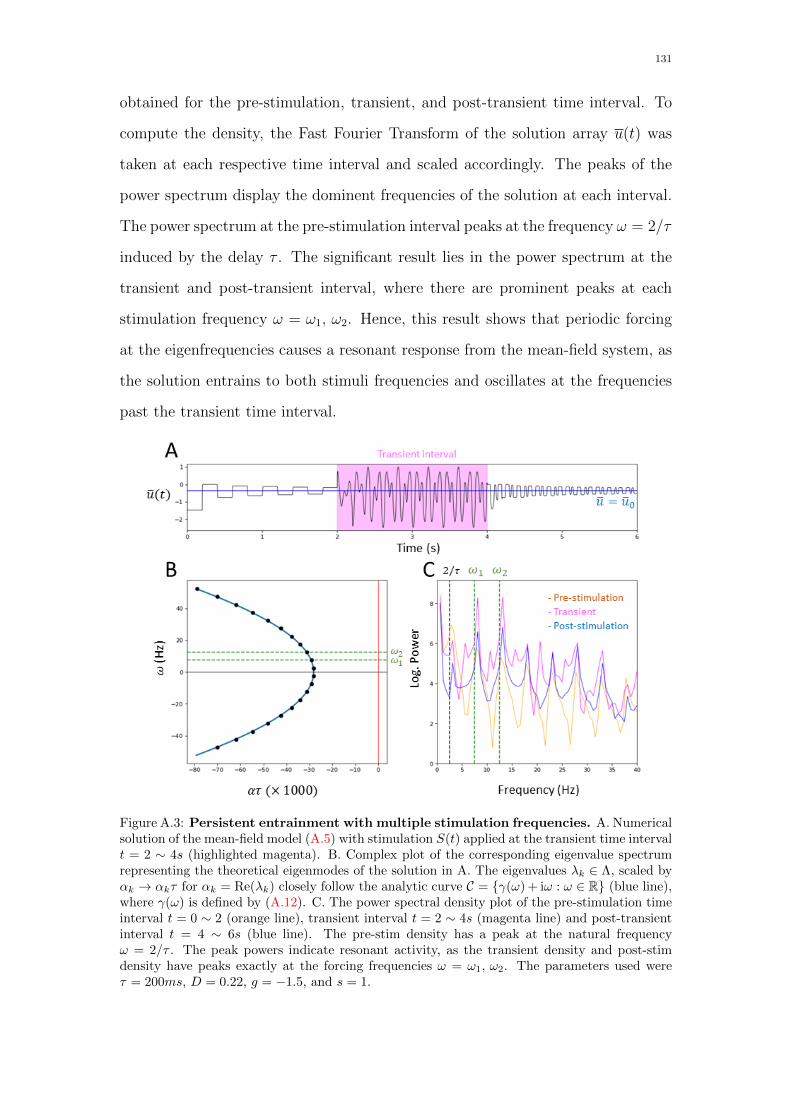
131
obtained for the pre-stimulation, transient, and post-transient time interval. To
compute the density, the Fast Fourier Transform of the solution array u(t) was
taken at each respective time interval and scaled accordingly. The peaks of the
power spectrum display the dominent frequencies of the solution at each interval.
The power spectrum at the pre-stimulation interval peaks at the frequency ω = 2/τ
induced by the delay τ . The significant result lies in the power spectrum at the
transient and post-transient interval, where there are prominent peaks at each
stimulation frequency ω = ω1, ω2. Hence, this result shows that periodic forcing
at the eigenfrequencies causes a resonant response from the mean-field system, as
the solution entrains to both stimuli frequencies and oscillates at the frequencies
past the transient time interval.
Figure A.3: Persistent entrainment with multiple stimulation frequencies. A. Numericalsolution of the mean-field model (A.5) with stimulation S(t) applied at the transient time intervalt = 2 ∼ 4s (highlighted magenta). B. Complex plot of the corresponding eigenvalue spectrumrepresenting the theoretical eigenmodes of the solution in A. The eigenvalues λk ∈ Λ, scaled byαk → αkτ for αk = Re(λk) closely follow the analytic curve C = γ(ω) + iω : ω ∈ R (blue line),where γ(ω) is defined by (A.12). C. The power spectral density plot of the pre-stimulation timeinterval t = 0 ∼ 2 (orange line), transient interval t = 2 ∼ 4s (magenta line) and post-transientinterval t = 4 ∼ 6s (blue line). The pre-stim density has a peak at the natural frequencyω = 2/τ . The peak powers indicate resonant activity, as the transient density and post-stimdensity have peaks exactly at the forcing frequencies ω = ω1, ω2. The parameters used wereτ = 200ms, D = 0.22, g = −1.5, and s = 1.

132

Appendix B
Proof of theorems
Here, we formally prove certain theorems applied throughout the thesis.
Proof of Theorem 7:
Proof. Equation (3.32) follows from the Fredholm determinant expansion
det
[I + β
M
N
]= 1 +
β
N
N∑i=1
Mii +
(β
N
)2 ∑1≤i<j≤N
det
Mii Mij
Mji Mjj
+
(β
N
)3 ∑1≤i<j<k≤N
det
Mii Mij Mik
Mji Mjj Mjk
Mki Mkj Mkk
+ · · ·+
(β
N
)NdetM
(B.1)
Taking the expectation of both sides of the above expression, only the first two
terms survive as the determinant of any submatrix of dimension d > 1 is a signed
permuted product of E[Mij] = µ. By definition of determinants, there are an equal
number of positive and negative signed permutations, causing the summation to
cancel out. Hence,
E(
det
[I + β
M
N
])= 1 +
β
N
N∑i=1
E[Mii] + 0 + · · ·+ 0 = 1 + βµ (B.2)
133

134 APPENDIX B. PROOF OF THEOREMS
By definition of the determinant, the summation in (B.1) consists of terms of the
formK∏i=1
Mki,ρ(ki) (B.3)
where K > 1 is the size of a sub-matrix in the summation (B.1) and 1 ≤ k1 < · · · <
kd ≤ N are the selected integers, and ρ is a permutation of the set k1, . . . , kd.
To prove equation (3.33), we have that the variance of any summation of random
variables X1, . . . , Xn is given by
Var(1 +X1 + · · ·+Xn) =n∑
i,j=1
Cov(Xi, Xj) (B.4)
where Cov(X, Y ) := E(XY )−EX ·EY is the covariance of random variables X, Y .
Hence, by taking the variance of the right-side expansion in (B.1), the variance of
det[I + βN−1M ] is a linear combination of terms of the form
Cov
(d1∏i=1
Mki,ρ1(ki),
d2∏j=1
M`j ,ρ2(`j)
)= σ2pµK−2p (B.5)
Here, d1, d2 ≤ N are the size of the two submatrices that contain the permuted
product terms, and K = d1 + d2 ≤ 2N . The integer p is the number of matching
terms ki, ρ1(ki) = `j, ρ2(`j), from which by the fact that the variables Mij are
i.i.d. and the definition of covariance, the equality in (B.5) follows. Var(det[I +
βN−1M ]) is a summation of the above terms (B.5) with each term multiplied by
the coefficient
sgn(ρ1) · sgn(ρ2)
(β
N
)K(B.6)
where sgn(ρ) ∈ −1, 1 is the sign of permutation ρ. The integer αK,p is the
signed number of terms given by (B.5) with total subdimension K = d1 + d2 and
p number of matching variables. In the special case that µ = 0, the only terms
given by (B.5) that survive are the ones that completely match. That is, terms
with d1 = d2, ρ1 = ρ2, ki = `i for all i, from which the coefficient αK,p is the
number of permutations in the determinant of each submatrix with dimension p.
This results in (3.34).

135
Proof of Theorem 9:
The Kuramoto model (4.2) and plasticity rule (4.3) with adaptive delays can be
expressed as an N+N2-dimensional system of oscillators θ(t) := (θi(t))1≤i≤N ∈ RN
and a matrix of delays τ (t) ∈ RN×N+ , defined by the state-dependent DDEs
θ(t) = F (θt, τ (t)) (B.7)
τ (t) = G(θ(t), τ (t)) (B.8)
where θt ∈ C := ([−r, 0],RN) defined by θt(s) = θ(t + s), s ∈ [−r, 0], and C
is the space of all continuous functions from interval [−r, 0] for some r > 0.
Here, F : C × RN×N+ → RN is the function whose ith co-ordinate Fi(θt, τ (t))
is given by (4.2) and G : RN × RN×N+ → RN×N
+ is the function whose ijth co-
ordinate Gij(θi(t), θj(t), τij(t)) is given by (4.3). Assuming the solutions θ(t), τ (t)
exist, each delay solution τ (t) is bounded for all t ≥ 0. This is clear since given
τij(t) > τ 0ij + κ, it must hold that τ ′ij(t) < 0. Hence, it suffices to define the space
C with any r > maxi,jτ 0ij+ κ.
Denote C1 ⊂ C to be the subspace of all continuously differentiable functions.
Let θ0(s) = ϕ(s) for some C1 initial function ϕ : [−r, 0] → RN and τ (0) =
τ 0 ∈ RN×N+ be the initial delays. Since (B.8) is a system of Ordinary Differential
Equations, τ (t) is independent of initial values on t < 0. Hence, we represent
an initial function for τ (t) with an initial point τ 0 ∈ RN×N+ . Existence and
uniqueness of solution (θ(t), τ (t)) follows by theorems in [25] given that both
F,G are continuously differentiable functions over (ϕ, τ 0) ∈ C1 ×RN×N+ . The ith
co-ordinate Fi(ϕ, τ0) is a linear combination of terms sin(ϕj(τ
0ij) − ϕi), which is
continuously differentiable over ϕ ∈ C1. G is continuously differentiable given the
Heaviside function H(τ) is smooth.

136

Appendix C
Smooth adjustments to functions
In accordance to Theorem 9 and similar theorems regarding DDEs found in [25,
76], existence and uniqueness of solutions are not guaranteed unless the vector
functionals f(t, xt) are smooth. Hence, we define the functions in the Kuramoto
model (4.2) and plasticity rule (4.3) for adaptive delays τij = τij(t). We define the
smooth mollifier function h : R→ R by
h(t) =
exp(−(x+ 1)−2) · exp(−(x− 1)−2) if − 1 < t < 1
0 otherwise
(C.1)
Then, we express the smooth Heavyside function Hε(τ) with small ε is defined
with respect to a smooth mollifier function h : R→ R as
Hε(τ) =
∫ τ
0h(−1 + 2ε−1s ds)∫ ε
0h(−1 + 2ε−1s) ds
if τ > 0
0 otherwise
(C.2)
Similarly, we can define the smoothly decaying connection term aij(t) as given in
(4.41) by writing
aij(t) =
∫ t−tinj,s0
h(−1 + 2s/(tinj,f − tinj,s)) ds∫ tinj,f−tinj,s0
h(−1 + 2s/(tinj,f − tinj,s)) dstinj,s < t < tinj,f (C.3)
and aij(t) = 1 for t < tinj,s, aij(t) = 0 for t > tinj,f , from which aij(t) ∈ [0, 1] and
decreases on interval (tinj,s, tinj,f ). From this construction, H(τ), aij(t) are both
137

138 APPENDIX C. SMOOTH ADJUSTMENTS TO FUNCTIONS
C∞ functions.
Even with existence and uniqueness of solutions of DDE systems, we may not
have nicely behaving solutions unless we also have sufficient smoothness in the
initial conditions. For the Kuramoto model with a single delay τ 0ij, we are able to
make adjustments to the history functions ϕi(t), where θi(t) = ϕi(t) for t ≤ 0, such
that they satisfy the necessary condition (4.37). While solutions θi(t) exist and
are unique by Theorem 9 without the history functions satisfying (4.37), we are
not guaranteed to have reasonably behaving solutions unless we have continuity
of θ′i(t) at t = 0. For details on this, see [72, 76]. This is also a necessary condition
for providing accurate numerical simulations, as the interpolation procedure in
dde23 and ddesd rely on θ′i(t) being continuous everywhere.
For the numerical simulations regarding the Kuramoto model with single base-
line (initial) delay τ 0ij = τ 0, we consider the linear initial functions ϕi(t) = Ω0 +ϕ0
i ,
i ≤ N , parametrized by initial frequency Ω0 ∈ R and phase offsets (ϕ01, . . . , ϕ
0N) ∈
RN . As discussed above, we require that our linear initial function to be contin-
uously differentiable at t = 0. Given any initial C1 function ϕi(t) for θi(t), we
define the modified C1 function ϕi(t) of ϕi(t) for each i ≤ N that is continuously
differentiable as follows. We can obtain the modified slope ~v ∈ RN by imposing
the following condition on ϕi(t)
vi = ω0 +g
N
N∑i=1
sin(ϕj(−τ 0)− ϕi(0)) (C.4)
Then, for each i we define the cubic polynomial pi : R→ R that interpolates ϕi(t)
between t = 0,−τ 0 using the modified slope. That is, pi(t) = ϕi(t) at t = 0,−τ 0
and p′i(0) = vi, p′i(−τ 0) = ϕi(−τ 0). Then, the modified initial function ϕi(t) is
given by
ϕi(t) =
ϕi(t) t < −τ 0
pi(t) −τ 0 ≤ t ≤ 0
(C.5)
for i ≤ N . All numerical trials for the Kuramoto model with single initial delay
were conducted using the corresponding modified functions ϕi(t) of ϕi(t) = Ω0t+
139
ϕ0i , i ≤ N . Otherwise, the unmodified linear functions ϕi(t) were used.

140

Appendix D
Numerical Methods
Here we discuss how numerical functions were implemented to provide solutions to
implicit equations and solve delay differential equations. All numerical simulations
were done through MATLAB, and all numerical arrays were plotted through the
matplotlib package in python. All non-analytically solvable integrals∫ baf(x) dx
were evaluated with the integral function from MATLAB.
To find points λ ∈ R or λ ∈ C that solve the root equation F (λ) = 0, we apply
the fminsearch function from MATLAB as follows. To search for solutions λ ∈ C,
we define the logorithmic error E(λ) := log10 |F (λ)| and rectangular search region
R = u + iv : |u| ≤ uL, |v| ≤ vL. At evenly spaced mesh points λp ∈ R so that
we’re taking Mu ×Mv points, we compute the error E(λp). At every point λP
whose error is within a certain tolerance E(λp) < tol, we conduct an fminsearch
for a local minima λ = λmin that minimizes E(λ) starting at λp. All unique
located points λmin following a set number of iterations iter are the numerically
approximated solutions to F (λ) = 0 with error |F (λmin)|. The same procedure
is done when searching for real-values λ ∈ R and fixed-point equations λ = G(λ)
by taking F (λ) = λ − G(λ). Typical search parameter values range as follows.
We take tol ∈ [−5, 1], depending on how thorough and quick the search needs to
be done, and the partition size for λP ∈ R is in the range Mu, Mv ∈ [50, 100].
The number of iterations is set to iter ∈ [2000, 2500] for all approximations. All
fminsearch estimates on each shown figure are graphed with view limits within
141

142 APPENDIX D. NUMERICAL METHODS
the rectangular region R.
Numerical trajectories for each DDE were obtained as follows. For the non-
linear mean-field equation (A.5), the dde23 function was implemented to obtain
the solution array u(t). For the Kuramoto model with static delays (3.5), the
dde23 function was implemented to obtain the solution arrays θi(t), i ≤ N and
derivative arrays θ′i(t), i ≤ N . For the Kuramoto model (4.2) with adaptive delays
(4.3), the ddesd function was implemented. Here, given the large-dimensional
case as in Section 4.5, the NormControl option was toggled ‘on’, for which the
integration step is determined based on control error relative to the norm of the
solution θi(t), τij(t).
For the exact scripts used to generate each figure and data set, we refer the
reader to https://github.com/parkseo7/DissertationCode.git.

List of symbols
The following is a full list of notations used throughout the dissertation:
• R+ = [0,∞)
• RN+ = x ∈ RN : xi ∈ R+
• (Rm)N = (x1, . . . , xN) : xi ∈ Rm
• C([−r, 0],Rn) = f : [−r, 0]→ RN , f continuous
• S is the unit circle
• T = [−π, π) mod 2π ' S1
•dy
dt= y(t) = y′(t) is the first-derivative of function y : R→ RN at time t.
• τ =
τ11 · · · τ1N
.... . .
...
τN1 · · · τNN
∈ RN×N+
• E[f(X)] is the expected value of random variable f(X).
• I is the N -dimensional square identity matrix.
• Ψλ,N = I+ βλMλN is the matrix for stability eigenvalues satisfying det[Ψλ,N ] = 0
• s. log10(x) = sign(x) · log10(1 + |x|)
• Ω = 1N
∑Ni=1
∫ Tt−T θ
′i(t) dt
The following abbreviations are used throughout the dissertation:
• WCON: Weakly coupled oscillator network
• i.i.d: independently and identically distributed
143

144

Bibliography
[1] Isam Al-Darabsah and Sue Campbell. “A phase model with large time delayed coupling”.
In: Physica D: Nonlinear Phenomena (May 2020), p. 132559. doi: 10.1016/j.physd.
2020.132559.
[2] Sankaraleengam Alagapan et al. “Modulation of Cortical Oscillations by Low-Frequency
Direct Cortical Stimulation Is State-Dependent”. In: PLoS biology 14 (Mar. 2016), e1002424.
doi: 10.1371/journal.pbio.1002424.
[3] John E. Hall Arthur C. Guyton. Guyton and Hall Textbook of Medical Physiology - 11th-Ed.
Jan. 2005.
[4] F. Atay. “Distributed delays facilitate amplitude death of coupled oscillators”. In: Physical
Review Letters, v.91 (2003) 91 (Jan. 2003).
[5] Franziska Auer, Stavros Vagionitis, and Tim Czopka. “Evidence for Myelin Sheath Re-
modeling in the CNS Revealed by In Vivo Imaging”. In: Current Biology 28 (Feb. 2018).
doi: 10.1016/j.cub.2018.01.017.
[6] Marie E Bechler, Matthew Swire, and Charles Ffrench-Constant. “Intrinsic and adaptive
myelination - a sequential mechanism for smart wiring in the brain”. English. In: Devel-
opmental neurobiology 78.2 (Aug. 2017), pp. 68–79. issn: 1932-8451. doi: 10.1002/dneu.
22518.
[7] Sonya Bells et al. “Changes in White Matter Microstructure Impact Cognition by Disrupt-
ing the Ability of Neural Assemblies to Synchronize”. In: The Journal of Neuroscience 37
(July 2017), pp. 0560–17. doi: 10.1523/JNEUROSCI.0560-17.2017.
[8] Dwight Bergles, Ronald Jabs, and Christian Steinhauser. “Neuron-glia synapses in the
brain”. In: Brain research reviews 63 (Dec. 2009), pp. 130–7. doi: 10.1016/j.brainresrev.
2009.12.003.
[9] Michael Breakspear, Stewart Heitmann, and Andreas Daffertshofer. “Generative Models of
Cortical Oscillations: Neurobiological Implications of the Kuramoto Model”. In: Frontiers
145

146 BIBLIOGRAPHY
in Human Neuroscience 4 (2010), p. 190. issn: 1662-5161. doi: 10.3389/fnhum.2010.
00190. url: https://www.frontiersin.org/article/10.3389/fnhum.2010.00190.
[10] Gyorgy Buzsaki. Rhythms of The Brain. Jan. 2009, xiv, 448 p. isbn: 9780195301069 (alk.
paper) 0195301064 (alk. paper). doi: 10.1093/acprof:oso/9780195301069.001.0001.
[11] Gyorgy Buzsaki, Costas Anastassiou, and Christof Koch. “The origin of extracellular fields
and currents—EEG, ECoG, LFP and spikes”. In: Nature reviews. Neuroscience 13 (May
2012), pp. 407–20. doi: 10.1038/nrn3241.
[12] Gyorgy Buzsaki. “Theta Oscillations in the Hippocampus”. In: Neuron 33.3 (2002), pp. 325
–340. issn: 0896-6273. doi: https://doi.org/10.1016/S0896-6273(02)00586-X. url:
http://www.sciencedirect.com/science/article/pii/S089662730200586X.
[13] Joana Cabral et al. “Exploring mechanisms of spontaneous MEG functional connectivity:
How delayed network interactions lead to structured amplitude envelopes of band-pass
filtered oscillations.” In: NeuroImage 90 (Dec. 2013). doi: 10.1016/j.neuroimage.2013.
11.047.
[14] Kenneth L. Cooke and Wenzhang Huang. “On the Problem of Linearization for State-
Dependent Delay Differential Equations”. In: Proceedings of the American Mathematical
Society 124.5 (1996), pp. 1417–1426. issn: 00029939, 10886826.
[15] Otti D’Huys et al. “Synchronization properties of network motifs: Influence of coupling
delay and symmetry”. In: Chaos (Woodbury, N.Y.) 18 (Oct. 2008), p. 037116. doi: 10.
1063/1.2953582.
[16] R Douglas Fields. “A new mechanism of nervous system plasticity: Activity-dependent
myelination”. In: Nature Reviews Neuroscience 16 (Nov. 2015), pp. 756–767. doi: 10.
1038/nrn4023.
[17] Matthew G. Earl and Steven H. Strogatz. “Synchronization in oscillator networks with
delayed coupling: A stability criterion”. In: Phys. Rev. E 67 (3 2003), p. 036204. doi:
10.1103/PhysRevE.67.036204.
[18] Vıctor Eguıluz et al. “Structural and functional networks in complex systems with de-
lay”. In: Physical review. E, Statistical, nonlinear, and soft matter physics 83 (May 2011),
p. 056113. doi: 10.1103/PhysRevE.83.056113.
[19] G.B. Ermentrout. “Oscillator death in populations of “all to all” coupled nonlinear oscilla-
tors”. In: Physica D: Nonlinear Phenomena 41.2 (1990), pp. 219 –231. issn: 0167-2789. doi:
https://doi.org/10.1016/0167-2789(90)90124-8. url: http://www.sciencedirect.
com/science/article/pii/0167278990901248.

BIBLIOGRAPHY 147
[20] Marc Ford et al. “Tuning of Ranvier node and internode properties in myelinated axons
to adjust action potential timing”. In: Nature Communications 6:8073 (Aug. 2015). doi:
10.1038/ncomms9073.
[21] Pascal Fries. “Neuronal Gamma-Band Synchronization as a Fundamental Process in Cor-
tical Computation”. In: Annual review of neuroscience 32 (Apr. 2009), pp. 209–24. doi:
10.1146/annurev.neuro.051508.135603.
[22] Rafael G. Almeida and David A. Lyons. “On Myelinated Axon Plasticity and Neuronal
Circuit Formation and Function”. In: The Journal of Neuroscience 37.42 (Oct. 2017),
pp. 10023–10034. doi: 10.1523/JNEUROSCI.3185-16.2017.
[23] Matthew Glasser and David Van Essen. “Mapping Human Cortical Areas in vivo Based
on Myelin Content as Revealed by T1- and T2-weighted MRI”. In: The Journal of neuro-
science : the official journal of the Society for Neuroscience 31 (Aug. 2011), pp. 11597–616.
doi: 10.1523/JNEUROSCI.2180-11.2011.
[24] L.F. Haas. “Hans Berger (1873–1941), Richard Caton (1842–1926), and electroencephalog-
raphy”. In: Journal of neurology, neurosurgery, and psychiatry 74 (Feb. 2003), p. 9. doi:
10.1136/jnnp.74.1.9.
[25] Jack K. Hale and S. M. Verduyn Lunel. Introduction to Functional Differential Equations.
New York: Springer-Verlag, 1993.
[26] Jasmeet Hayes, Erin Bigler, and Mieke Verfaellie. “Traumatic Brain Injury as a Disorder of
Brain Connectivity”. In: Journal of the International Neuropsychological Society in press
(Nov. 2015). doi: 10.1017/S1355617715000740.
[27] Robert Hill, Alice Li, and Jaime Grutzendler. “Lifelong cortical myelin plasticity and age-
related degeneration in the live mammalian brain”. In: Nature neuroscience 21 (May 2018).
doi: 10.1038/s41593-018-0120-6.
[28] A. Hodgkin and A. Huxley. “A quantitative description of membrane current and its
application to conduction and excitation in nerve”. In: The Journal of Physiology 117
(1952).
[29] Shir Hofstetter et al. “Short-Term Learning Induces White Matter Plasticity in the Fornix”.
In: The Journal of neuroscience : the official journal of the Society for Neuroscience 33
(July 2013), pp. 12844–50. doi: 10.1523/JNEUROSCI.4520-12.2013.
[30] Livia de Hoz and Mikael Simons. “The emerging functions of oligodendrocytes in regu-
lating neuronal network behaviour”. In: BioEssays 37 (Jan. 2015). doi: 10.1002/bies.
201400127.

148 BIBLIOGRAPHY
[31] Ethan Hughes et al. “Myelin remodeling through experience-dependent oligodendrogenesis
in the adult somatosensory cortex”. In: Nature neuroscience 21 (May 2018). doi: 10.1038/
s41593-018-0121-5.
[32] Tomoko Ishibashi et al. “Astrocytes Promote Myelination in Response to Electrical Im-
pulses”. In: Neuron 49 (Apr. 2006), pp. 823–32. doi: 10.1016/j.neuron.2006.02.006.
[33] Taishi Iwasaki et al. “Estimation of neural connections from partially observed neural
spikes”. In: Neural Networks 108 (Nov. 2017). doi: 10.1016/j.neunet.2018.07.019.
[34] E.M. Izhikevich. “Which Model to Use for Cortical Spiking Neurons?” In: Neural Networks,
IEEE Transactions on 15 (Oct. 2004), pp. 1063 –1070. doi: 10.1109/TNN.2004.832719.
[35] Eugene Izhikevich. “Phase Models With Explicit Time Delays”. In: Physical Review E 58
(May 1998). doi: 10.1103/PhysRevE.58.905.
[36] Eugene Izhikevich. “Simple model of Spiking Neurons”. In: IEEE transactions on neural
networks / a publication of the IEEE Neural Networks Council 14 (Feb. 2003), pp. 1569–
72. doi: 10.1109/TNN.2003.820440.
[37] Eugene M. Izhikevich and Frank C. Hoppensteadt. Weakly Connected Neural Networks.
Springer-Verlag New York, 1997. doi: 10.1007/978-1-4612-1828-9.
[38] Florian Kasten, James Dowsett, and Christoph Herrmann. “Sustained Aftereffect of α-
tACS Lasts Up to 70 min after Stimulation”. In: Frontiers in Human Neuroscience 10
(May 2016). doi: 10.3389/fnhum.2016.00245.
[39] Christoph Kayser, Nikos Logothetis, and Stefano Panzeri. “Millisecond encoding precision
of auditory cortex neurons”. In: Proceedings of the National Academy of Sciences of the
United States of America 107 (Sept. 2010), pp. 16976–81. doi: 10.1073/pnas.1012656107.
[40] Y. Kuramoto. Chemical Oscillations, Waves, and Turbulence. Berlin, New York: Springer-
Verlag, 1984.
[41] Jeremie Lefebvre et al. “Stimulus Statistics Shape Oscillations in Nonlinear Recurrent
Neural Networks”. In: Journal of Neuroscience 35 (Feb. 2015), pp. 2895–2903. doi: 10.
1523/JNEUROSCI.3609-14.2015.
[42] Mark Lichtner, Matthias Wolfrum, and Serhiy Yanchuk. “The Spectrum of Delay Differ-
ential Equations with Large Delay”. In: SIAM J. Math. Analysis 43 (Jan. 2011), pp. 788–
802. doi: 10.1137/090766796.

BIBLIOGRAPHY 149
[43] Jia Liu et al. “White Matter Plasticity in Anxiety: Disruption of Neural Network Syn-
chronization During Threat-Safety Discrimination”. In: Frontiers in Cellular Neuroscience
14 (2020), p. 351. issn: 1662-5102. doi: 10.3389/fncel.2020.587053. url: https:
//www.frontiersin.org/article/10.3389/fncel.2020.587053.
[44] Vıctor J. Lopez-Madrona et al. “Gamma oscillations coordinate different theta rhythms
in the hippocampus”. In: bioRxiv (2018). doi: 10.1101/418434. eprint: https://www.
biorxiv.org/content/early/2018/09/14/418434.full.pdf. url: https://www.
biorxiv.org/content/early/2018/09/14/418434.
[45] Manabu Makinodan et al. “A Critical Period for Social Experience-Dependent Oligoden-
drocyte Maturation and Myelination”. In: Science (New York, N.Y.) 337 (Sept. 2012),
pp. 1357–60. doi: 10.1126/science.1220845.
[46] Andreas Mierau, Wolfgang Klimesch, and Jeremie Lefebvre. “State-Dependent Alpha Peak
Frequency Shifts: Experimental Evidence, Potential Mechanisms and Functional Implica-
tions”. In: Neuroscience 360 (July 2017). doi: 10.1016/j.neuroscience.2017.07.037.
[47] Michelle Monje. “Myelin Plasticity and Nervous System Function”. In: Annual Review of
Neuroscience 41 (July 2018), pp. 61–76. doi: 10.1146/annurev-neuro-080317-061853.
[48] Christopher Mount and Michelle Monje. “Wrapped to Adapt: Experience-Dependent Myeli-
nation”. In: Neuron 95 (Aug. 2017), pp. 743–756. doi: 10.1016/j.neuron.2017.07.009.
[49] Richard Naud and Andre Longtin. “Linking demyelination to compound action potential
dispersion with a spike-diffuse-spike approach”. In: The Journal of Mathematical Neuro-
science 9 (Dec. 2019). doi: 10.1186/s13408-019-0071-6.
[50] Toralf Neuling, Stefan Rach, and Christoph Herrmann. “Orchestrating neuronal networks:
sustained after-effects of transcranial alternating current stimulation depend upon brain
states”. In: Frontiers in human neuroscience 7 (Apr. 2013), p. 161. doi: 10.3389/fnhum.
2013.00161.
[51] Hoi H. Nguyen and Van Vu. “Random matrices: Law of the determinant”. In: The Annals
of Probability 42.1 (2014), 146–167. issn: 0091-1798. doi: 10.1214/12- aop791. url:
http://dx.doi.org/10.1214/12-AOP791.
[52] Rabiya Noori et al. “Activity-dependent myelination: A glial mechanism of oscillatory
self-organization in large-scale brain networks”. In: Proceedings of the National Academy
of Sciences 117 (June 2020), p. 201916646. doi: 10.1073/pnas.1916646117.
[53] M. Okun, A. Naim, and I. Lampl. “The Subthreshold Relation between Cortical Local
Field Potential and Neuronal Firing Unveiled by Intracellular Recordings in Awake Rats”.
In: The Journal of Neuroscience 30 (2010), pp. 4440 –4448.

150 BIBLIOGRAPHY
[54] S. Pajevic, P.J. Basser, and R.D. Fields. “Role of myelin plasticity in oscillations and
synchrony of neuronal activity”. In: Neuroscience 276 (2014). Secrets of the CNS White
Matter, pp. 135 –147. issn: 0306-4522. doi: https://doi.org/10.1016/j.neuroscience.
2013.11.007. url: http://www.sciencedirect.com/science/article/pii/S0306452213009470.
[55] Antonis Papachristodoulou and Ali Jadbabaie. “Synchronization in Oscillator Networks:
Switching Topologies and Non-homogeneous Delays”. In: Proceedings of the 44th IEEE
Conference on Decision and Control (2005), pp. 5692–5697.
[56] Seong Park and Jeremie Lefebvre. “Synchronization and resilience in the Kuramoto white
matter network model with adaptive state-dependent delays”. In: (Aug. 2020). doi: 10.
1101/2020.08.25.266841.
[57] Seong Park et al. “Persistent Entrainment in Non-linear Neural Networks With Memory”.
In: Frontiers in Applied Mathematics and Statistics 4 (Aug. 2018). doi: 10.3389/fams.
2018.00031.
[58] Spase Petkoski and Viktor Jirsa. “Transmission time delays organize the brain network
synchronization”. In: Philosophical Transactions of the Royal Society A: Mathematical,
Physical and Engineering Sciences 377 (Sept. 2019), p. 20180132. doi: 10.1098/rsta.
2018.0132.
[59] Spase Petkoski, J. Matias Palva, and Viktor Jirsa. “Phase-lags in large scale brain synchro-
nization: Methodological considerations and in-silico analysis”. In: PLOS Computational
Biology 14 (July 2018), e1006160. doi: 10.1371/journal.pcbi.1006160.
[60] Adrian Ponce-Alvarez et al. “Resting-State Temporal Synchronization Networks Emerge
from Connectivity Topology and Heterogeneity”. In: PLoS computational biology 11 (Feb.
2015), e1004100. doi: 10.1371/journal.pcbi.1004100.
[61] D. Reddy, Abhijit Sen, and G. Johnston. “Time Delay Induced Death in Coupled Limit Cy-
cle Oscillators”. In: Physical Review Letters 80 (May 1998). doi: 10.1103/PhysRevLett.
80.5109.
[62] Francisco Rodrigues et al. “The Kuramoto model in complex networks”. In: Physics Re-
ports 610 (Jan. 2016), pp. 1–98. doi: 10.1016/j.physrep.2015.10.008.
[63] Raul Rojas. Neural Networks - A Systematic Introduction. Springer, 1996.
[64] Kunimochi Sakamoto. “Invariant manifolds in singular perturbation problems for ordi-
nary differential equations”. In: Proceedings of the Royal Society of Edinburgh: Section A
Mathematics 116.1-2 (1990), 45–78. doi: 10.1017/S0308210500031371.

BIBLIOGRAPHY 151
[65] Emilio Salinas and Terrence Sejnowski. “Impact of Correlated Synaptic Input on Output
Firing Rate and Variability in Simple Neuronal Models”. In: The Journal of neuroscience
: the official journal of the Society for Neuroscience 20 (Sept. 2000), pp. 6193–209.
[66] Patrick Steadman et al. “Disruption of Oligodendrogenesis Impairs Memory Consolidation
in Adult Mice”. In: Neuron 105 (Nov. 2019). doi: 10.1016/j.neuron.2019.10.013.
[67] Steven H. Strogatz. “From Kuramoto to Crawford: exploring the onset of synchronization
in populations of coupled oscillators”. In: Physica D: Nonlinear Phenomena 143.1 (2000),
pp. 1 –20. issn: 0167-2789. doi: 10.1016/S0167-2789(00)00094-4.
[68] Giulio srubek tomassy et al. “Distinct Profiles of Myelin Distribution Along Single Axons
of Pyramidal Neurons in the Neocortex”. In: Science (New York, N.Y.) 344 (Apr. 2014),
pp. 319–24. doi: 10.1126/science.1249766.
[69] Peter Uhlhaas and Wolf Singer. “The Development of Neural Synchrony and Large-Scale
Cortical Networks During Adolescence: Relevance for the Pathophysiology of Schizophrenia
and Neurodevelopmental Hypothesis”. In: Schizophrenia bulletin 37 (May 2011), pp. 514–
23. doi: 10.1093/schbul/sbr034.
[70] Peter Uhlhaas et al. “Neural synchrony and the development of cortical networks”. In:
Trends in cognitive sciences 14 (Feb. 2010), pp. 72–80. doi: 10.1016/j.tics.2009.12.
002.
[71] Mateo Velez-Fort et al. “Postnatal Switch from Synaptic to Extrasynaptic Transmission
between Interneurons and NG2 Cells”. In: The Journal of neuroscience : the official journal
of the Society for Neuroscience 30 (May 2010), pp. 6921–9. doi: 10.1523/JNEUROSCI.
0238-10.2010.
[72] Hans-Otto Walther. “The solution manifold and C1-smoothness for differential equations
with state-dependent delay”. In: Journal of Differential Equations 195 (Nov. 2003), pp. 46–
65. doi: 10.1016/j.jde.2003.07.001.
[73] Lei Wang et al. “Ionic mechanisms underlying tonic and phasic firing behaviors in retinal
ganglion cells: A model study”. In: Channels (Austin, Tex.) 8 (Mar. 2014). doi: 10.4161/
chan.28012.
[74] John Welsh, Edward Ahn, and Dimitris Placantonakis. “Is autism due to brain desynchro-
nization? Int J Dev Neurosci”. In: International journal of developmental neuroscience :
the official journal of the International Society for Developmental Neuroscience 23 (Apr.
2005), pp. 253–63. doi: 10.1016/j.ijdevneu.2004.09.002.

152 BIBLIOGRAPHY
[75] Jill Williamson and David Lyons. “Myelin Dynamics Throughout Life: An Ever-Changing
Landscape?” In: Frontiers in Cellular Neuroscience 12 (Nov. 2018), p. 424. doi: 10.3389/
fncel.2018.00424.
[76] Jianhong Wu. “Chapter 5 Functional Differential Equations with State-Dependent Delays:
Theory and Applications”. In: Handbook of Differential Equations: Ordinary Differential
Equations 3 (Dec. 2006). doi: 10.1016/S1874-5725(06)80009-X.
[77] M. K. Stephen Yeung and Steven H. Strogatz. “Time Delay in the Kuramoto Model
of Coupled Oscillators”. In: Phys. Rev. Lett. 82 (3 1999), pp. 648–651. doi: 10.1103/
PhysRevLett.82.648.
[78] Maggie S.Y. Yeung et al. “Dynamics of Oligodendrocyte Generation and Myelination in the
Human Brain”. In: Cell 159 (Nov. 2014), pp. 766–74. doi: 10.1016/j.cell.2014.10.011.