adaptive second order sliding mode control … · sliding mode controller. the integral sliding...
TRANSCRIPT

ADAPTIVE SECOND ORDER SLIDING MODE CONTROL STRATEGIES
FOR UNCERTAIN SYSTEMS
SANJOY MONDAL
ADAPTIVE SECOND ORDER SLIDING MODE
CONTROL STRATEGIES FOR UNCERTAIN
SYSTEMS
A
Thesis Submitted
in Partial Fulfilment of the Requirements
for the Degree of
DOCTOR OF PHILOSOPHY
By
SANJOY MONDAL
Department of Electronics and Electrical Engineering
Indian Institute of Technology Guwahati
Guwahati - 781 039, INDIA.
July, 2012
Certificate
This is to certify that the thesis entitled “ADAPTIVE SECOND ORDER SLIDING MODE
CONTROL STRATEGIES FOR UNCERTAIN SYSTEMS”, submitted by Sanjoy Mondal
(08610202), a research scholar in the Department of Electronics and Electrical Engineering, Indian
Institute of Technology Guwahati, for the award of the degree of Doctor of Philosophy, is a record
of an original research work carried out by him under my supervision and guidance. The thesis has
fulfilled all requirements as per the regulations of the Institute and in my opinion has reached the
standard needed for submission. The results embodied in this thesis have not been submitted to any
other University or Institute for the award of any degree or diploma.
Dated: Dr. Chitralekha Mahanta
Guwahati. Professor
Dept. of Electronics and Electrical Engg.
Indian Institute of Technology Guwahati
Guwahati - 781039, India.

To the memory of my father Ashok Kumar Mondal
Acknowledgement
First and foremost, I feel it as a great privilege in expressing my deepest and most sincere grati-
tude to my supervisor Dr. Chitralekha Mahanta, for her excellent guidance. Her kindness, dedication,
friendly accessibility and attention to details have been a great inspiration to me. My heartfelt thanks
to my supervisor for the unlimited support and patience shown to me. I would particularly like to
thank for all her help in patiently and carefully correcting all my manuscripts.
I am also very thankful to my doctoral committee members Prof. R. Bhattacharjee, Prof. S. Majhi
and Prof. S. K. Dwivedy for sparing their precious time to evaluate the progress of my work. Their
suggestions have been valuable. I would also like to thank other faculty members of EEE Dept. for
their kind help during my academic work. I am grateful to all the members of the research and tech-
nical staff of the department without whose help I could not have completed this thesis.
Thanks go out to all my friends in the Control and Instrumentation Laboratory. They have always
been around to provide useful suggestions, companionship and created a peaceful research environ-
ment.
My friends at IITG made my life joyful and were constant source of encouragement. Among my
friends, I would like to extend my special thanks to Ali, Senthil, Utkal, Kuntal, Om Prakash, Nagesh,
Asish, Rajib Panigharhi, Sayantan, Rajib Jana and Sanjeev. My work definitely would not have been
possible without their love and care which helped me to enjoy my new life in IITG. Special thanks also
go to Dola Govind Pradhan, Bajrangbali, Mandar, Mridul, Madhulika, Tausif, Basudev and Arghya
for their help during my stay.
My deepest gratitude goes to my family for the continuous love and support showered on me through-
out. The opportunities that they have given me and their unlimited sacrifices are the reasons for my
being where I am and what I have accomplished so far.
v
Abstract
The main objective of this thesis is to develop robust sliding mode control strategies for uncertain
systems. More specifically, the aim of this thesis is to develop sliding mode control schemes which are
successful in controlling systems affected by both matched and mismatched types of uncertainty. One
major drawback suffered by conventional sliding mode controllers is the presence of high frequency
oscillations in the control input known as chattering. Because of the discontinuous control action in
sliding mode controllers, chattering becomes an inherent undesired phenomenon. Apart from chatter-
ing, another disadvantage faced by conventional sliding mode controllers is their design prerequisite
of advance knowledge about the upper bound of the system uncertainty. This thesis is an attempt
to provide solution for these two main limitations of conventional first order sliding mode controllers.
The central focus of this thesis is to improve upon the existing sliding mode control techniques with
the prime objective of chattering mitigation. An adaptive gain tuning mechanism which can estimate
the uncertainty adaptively is proposed in this thesis. Hence prior knowledge about the upper bound
of system uncertainty is no longer a necessary requirement in the proposed adaptive sliding mode
controller. The basic idea of the proposed adaptive sliding mode controller is that the discontinuous
sign function is made to act on the time derivative of the control input and the actual control signal
obtained after integration is continuous and hence chattering is removed. The adaptive gain tuning
strategy ensures that the controller gain is not overestimated. Based upon the core idea of adaptive
sliding mode, various classes of sliding mode controllers are proposed in this thesis. In order to ensure
smooth control action throughout the entire operating range, this thesis proposes an adaptive integral
sliding mode controller. The integral sliding mode (ISM) algorithm eliminates the reaching phase.
Therefore, invariance towards matched disturbances can be ensured from the very beginning by using
this method. The proposed adaptive sliding mode control methodology is used to control nonlinear
multiple input multiple output (MIMO) systems which are highly cross-coupled. The proposed con-
vi
troller is used for stabilization as well as trajectory tracking of coupled MIMO systems affected by
both matched and mismatched uncertainty. Experimental studies are conducted on a single degree of
freedom (DOF) vertical take-off and landing (VTOL) aircraft system to study the real time perfor-
mance of the proposed adaptive sliding mode (SM) controller. The design prerequisite of the proposed
controller is complete knowledge about the state vector which is not available in this example. Hence
unavailable states of the 1 DOF VTOL are estimated by using an extended state observer (ESO). It is
a well established fact that finite time convergence of terminal sliding mode (TSM) control exists and
can be proved if a detailed mathematical analysis of its behaviour near the singularities is available.
However, TSM suffers from the drawback of chattering like in conventional first order sliding mode.
The proposed adaptive sliding mode strategy is used to design a terminal sliding mode controller for
linear and nonlinear uncertain systems. To improve the transient performance of uncertain systems,
a nonlinear sliding surface based adaptive chattering free sliding mode controller is proposed. The
nonlinear sliding surface changes the system’s closed loop damping ratio from its initial low value to
a final high value in accordance with the error magnitude. Hence fast initial response and gradually
diminishing overshoot are ensured. This thesis extends the nonlinear sliding surface based integral
sliding mode (ISM) controller to the discrete domain also where the controller consists of a nominal
control and ISM based discontinuous control. The nominal control is designed based on composite
nonlinear feedback (CNF) which varies the damping ratio of the closed loop system to ensure good
transient performance. The discontinuous control component rejects the matched disturbances and
model mismatches. Simulation studies are conducted involving linear and nonlinear, SISO and MIMO
systems affected by both matched and mismatched types of uncertainty and their results demonstrate
the effectiveness of the proposed adaptive chattering free sliding mode controller.
vii
Contents
List of Figures xi
List of Tables xv
List of Acronyms xv
List of Symbols xvii
List of Publications xix
1 Introduction 1
1.1 Introduction . . . . . . . . . . . . . . . . . . . . . . . . . . . . . . . . . . . . . . . . . . 2
1.2 Motivation and purpose . . . . . . . . . . . . . . . . . . . . . . . . . . . . . . . . . . . 3
1.3 Contributions of this Thesis . . . . . . . . . . . . . . . . . . . . . . . . . . . . . . . . . 5
1.4 Organization of the Thesis . . . . . . . . . . . . . . . . . . . . . . . . . . . . . . . . . . 5
2 Preliminary Concepts 8
2.1 Introduction . . . . . . . . . . . . . . . . . . . . . . . . . . . . . . . . . . . . . . . . . . 9
2.2 Variable Structure System and Sliding Mode . . . . . . . . . . . . . . . . . . . . . . . 9
2.3 Stability of the Sliding mode . . . . . . . . . . . . . . . . . . . . . . . . . . . . . . . . 11
2.4 Relative Degree in Sliding Mode . . . . . . . . . . . . . . . . . . . . . . . . . . . . . . 12
2.5 Order of the sliding mode . . . . . . . . . . . . . . . . . . . . . . . . . . . . . . . . . . 12
2.6 Finite time stability . . . . . . . . . . . . . . . . . . . . . . . . . . . . . . . . . . . . . 13
2.7 Chattering . . . . . . . . . . . . . . . . . . . . . . . . . . . . . . . . . . . . . . . . . . . 15
2.8 Summary . . . . . . . . . . . . . . . . . . . . . . . . . . . . . . . . . . . . . . . . . . . 17
3 Adaptive Integral Sliding Mode Controller 18
3.1 Introduction . . . . . . . . . . . . . . . . . . . . . . . . . . . . . . . . . . . . . . . . . . 19
3.2 Problem Definition . . . . . . . . . . . . . . . . . . . . . . . . . . . . . . . . . . . . . . 20
3.3 Design of adaptive integral sliding mode controller . . . . . . . . . . . . . . . . . . . . 21
viii
Contents
3.3.1 Finite time stabilization of an integrator chain system . . . . . . . . . . . . . . 22
3.3.2 Design of integral sliding mode controller . . . . . . . . . . . . . . . . . . . . . 22
3.3.3 Design of adaptive integral chattering free sliding mode controller . . . . . . . 24
3.4 Simulation Examples . . . . . . . . . . . . . . . . . . . . . . . . . . . . . . . . . . . . . 26
3.4.1 Adaptive integral chattering free sliding mode controller for the triple integrator
system . . . . . . . . . . . . . . . . . . . . . . . . . . . . . . . . . . . . . . . . . 26
3.4.2 Adaptive integral chattering free sliding mode controller for the single inverted
pendulum . . . . . . . . . . . . . . . . . . . . . . . . . . . . . . . . . . . . . . . 27
3.5 Summary . . . . . . . . . . . . . . . . . . . . . . . . . . . . . . . . . . . . . . . . . . . 29
4 Adaptive Sliding Mode Controller for Multiple Input Multiple Output (MIMO)Systems 30
4.1 Introduction . . . . . . . . . . . . . . . . . . . . . . . . . . . . . . . . . . . . . . . . . . 31
4.2 Adaptive sliding mode controller . . . . . . . . . . . . . . . . . . . . . . . . . . . . . . 32
4.2.1 Stability during the sliding mode . . . . . . . . . . . . . . . . . . . . . . . . . . 32
4.2.2 Design of the control law . . . . . . . . . . . . . . . . . . . . . . . . . . . . . . 34
4.2.3 Design of the adaptive tuning law . . . . . . . . . . . . . . . . . . . . . . . . . 35
4.3 The twin rotor MIMO System . . . . . . . . . . . . . . . . . . . . . . . . . . . . . . . . 37
4.3.1 TRMS Description . . . . . . . . . . . . . . . . . . . . . . . . . . . . . . . . . . 37
4.3.2 System Modeling . . . . . . . . . . . . . . . . . . . . . . . . . . . . . . . . . . . 38
4.3.3 Design of sliding mode controller for the TRMS horizontal subsystem . . . . . 43
4.3.4 Design of adaptive tuning law for the horizontal subsystem . . . . . . . . . . . 45
4.3.5 Stability during the sliding mode . . . . . . . . . . . . . . . . . . . . . . . . . . 46
4.3.6 Design of sliding mode controller for the TRMS vertical subsystem . . . . . . . 47
4.3.7 Design of adaptive tuning law for the vertical subsystem . . . . . . . . . . . . . 48
4.3.8 Stability of the sliding surface . . . . . . . . . . . . . . . . . . . . . . . . . . . . 49
4.3.9 Simulation results . . . . . . . . . . . . . . . . . . . . . . . . . . . . . . . . . . 51
4.3.10 Control parameters for the horizontal subsystem . . . . . . . . . . . . . . . . . 51
4.3.11 Control parameters for the vertical subsystem . . . . . . . . . . . . . . . . . . . 51
4.4 The vertical take-off and landing (VTOL) aircraft . . . . . . . . . . . . . . . . . . . . 56
4.4.1 Adaptive sliding mode controller design with PI sliding surface . . . . . . . . . 57
4.4.2 The adaptive PI sliding surface design . . . . . . . . . . . . . . . . . . . . . . . 59
ix
Contents
4.4.3 Effectiveness . . . . . . . . . . . . . . . . . . . . . . . . . . . . . . . . . . . . . 65
4.4.4 Simulation Results . . . . . . . . . . . . . . . . . . . . . . . . . . . . . . . . . . 66
4.5 Case study on 1 degree of freedom (DOF) vertical take-off and landing (VTOL) aircraft
system . . . . . . . . . . . . . . . . . . . . . . . . . . . . . . . . . . . . . . . . . . . . . 70
4.5.1 Linear extended state observer (LESO) design . . . . . . . . . . . . . . . . . . 71
4.5.2 Experimental Results . . . . . . . . . . . . . . . . . . . . . . . . . . . . . . . . 73
4.6 Summary . . . . . . . . . . . . . . . . . . . . . . . . . . . . . . . . . . . . . . . . . . . 78
5 Adaptive Terminal Sliding Mode Controller 80
5.1 Introduction . . . . . . . . . . . . . . . . . . . . . . . . . . . . . . . . . . . . . . . . . . 81
5.2 Design of chattering free adaptive terminal sliding mode controller . . . . . . . . . . . 82
5.3 Stabilization of a triple integrator system . . . . . . . . . . . . . . . . . . . . . . . . . 87
5.4 Tracking control of a robotic manipulator . . . . . . . . . . . . . . . . . . . . . . . . . 90
5.4.1 Effectiveness . . . . . . . . . . . . . . . . . . . . . . . . . . . . . . . . . . . . . 93
5.4.2 Simulation Studies . . . . . . . . . . . . . . . . . . . . . . . . . . . . . . . . . . 93
5.5 Summary . . . . . . . . . . . . . . . . . . . . . . . . . . . . . . . . . . . . . . . . . . . 101
6 Nonlinear Sliding Surface based Adaptive Sliding Mode Controller 102
6.1 Introduction . . . . . . . . . . . . . . . . . . . . . . . . . . . . . . . . . . . . . . . . . . 103
6.2 Adaptive chattering free sliding mode (SM) controller using nonlinear sliding surface . 104
6.2.1 Stability in sliding mode . . . . . . . . . . . . . . . . . . . . . . . . . . . . . . . 105
6.2.2 Choice of nonlinear function Υ(r, y) . . . . . . . . . . . . . . . . . . . . . . . . 109
6.2.3 Simulation Results . . . . . . . . . . . . . . . . . . . . . . . . . . . . . . . . . . 110
6.2.3.1 Time response of second order process with time delay . . . . . . . . 110
6.2.3.2 Comparison with adaptive SM controller using linear sliding surface . 112
6.2.4 Stabilization of an uncertain system . . . . . . . . . . . . . . . . . . . . . . . . 113
6.2.5 Performance comparison with third order sliding mode controller . . . . . . . . 117
6.3 Composite nonlinear feedback based discrete integral sliding mode controller . . . . . 121
6.3.1 Discrete ISM controller for linear system with matched uncertainty . . . . . . . 121
6.3.2 Composite nonlinear feedback (CNF) based controller design . . . . . . . . . . 124
6.3.3 Closed loop behavior and stability of the overall system . . . . . . . . . . . . . 126
6.3.4 Simulation Results . . . . . . . . . . . . . . . . . . . . . . . . . . . . . . . . . . 128
x
List of Figures
6.3.4.1 Single input single output (SISO) system . . . . . . . . . . . . . . . . 128
6.3.4.2 Comparison of the proposed discrete CNF-ISM controller with different
discrete ISM controllers . . . . . . . . . . . . . . . . . . . . . . . . . . 132
6.3.4.3 Multiple-input multiple-output (MIMO) system . . . . . . . . . . . . 133
6.4 Summary . . . . . . . . . . . . . . . . . . . . . . . . . . . . . . . . . . . . . . . . . . . 136
7 Conclusions and Scope for Future Work 138
7.1 Conclusions . . . . . . . . . . . . . . . . . . . . . . . . . . . . . . . . . . . . . . . . . . 139
7.2 Scope for future work . . . . . . . . . . . . . . . . . . . . . . . . . . . . . . . . . . . . 140
A Appendix 142
A.1 Modeling of 1 DOF VTOL Aircraft System . . . . . . . . . . . . . . . . . . . . . . . . 143
References 146
xi
List of Figures
2.1 Illustration of Filippov method . . . . . . . . . . . . . . . . . . . . . . . . . . . . . . . 11
2.2 The chattering effect . . . . . . . . . . . . . . . . . . . . . . . . . . . . . . . . . . . . . 16
3.1 State response with the proposed control law (3.22) . . . . . . . . . . . . . . . . . . . . 27
3.2 Control input with the proposed control law (3.22) . . . . . . . . . . . . . . . . . . . . 27
3.3 Sliding surface with the proposed control law (3.22) . . . . . . . . . . . . . . . . . . . 27
3.4 Estimated adaptive gain with the proposed control law (3.22) . . . . . . . . . . . . . . 27
3.5 System output with the proposed control law (3.22) . . . . . . . . . . . . . . . . . . . 28
3.6 Control input with the proposed control law (3.22) . . . . . . . . . . . . . . . . . . . . 28
3.7 Sliding manifold with the proposed control law (3.22) . . . . . . . . . . . . . . . . . . 29
3.8 Estimated adaptive gain with the proposed control law (3.22) . . . . . . . . . . . . . . 29
4.1 The twin rotor MIMO system (TRMS) [1] . . . . . . . . . . . . . . . . . . . . . . . . . 38
4.2 Step response of the TRMS using the proposed adaptive SM controller . . . . . . . . . 52
4.3 Adaptive gain parameter of proposed adaptive SM controller . . . . . . . . . . . . . . 53
4.4 Square wave response of the TRMS using the proposed adaptive sliding mode controller 54
4.5 Sine wave response of the TRMS using the proposed adaptive sliding mode controller 54
4.6 Position tracking using the proposed controller subjected to an external disturbance . 55
4.7 A typical sketch of a VTOL aircraft in the vertical plane [2]. . . . . . . . . . . . . . . 57
4.8 State responses with the method proposed by Wen and Cheng [3] . . . . . . . . . . . . 67
4.9 Control inputs with the method proposed by Wen and Cheng [3] . . . . . . . . . . . . 68
4.10 State responses using the proposed adaptive sliding mode controller . . . . . . . . . . 68
4.11 Control inputs using the proposed adaptive sliding mode controller . . . . . . . . . . . 69
4.12 Estimated parameters using the proposed adaptive sliding mode controller . . . . . . 69
4.13 Sliding surface and sliding manifold using the proposed adaptive sliding mode controller 70
xii
List of Figures
4.14 QNET VTOL trainer on ELVIS II . . . . . . . . . . . . . . . . . . . . . . . . . . . . . 73
4.15 Angular position (x1) obtained by using the proposed adaptive sliding mode controller 75
4.16 Angular velocity (x2) obtained by using the proposed adaptive sliding mode controller 75
4.17 Sliding surface s obtained by using the proposed adaptive sliding mode controller . . . 76
4.18 Control input u obtained by using the proposed adaptive sliding mode controller . . . 76
4.19 Adaptive gain (T ) obtained by using the proposed adaptive sliding mode controller . . 77
4.20 Experimental results using the proposed method when parameters are changed by 25% 77
5.1 State response and control input with the controller proposed in [4] . . . . . . . . . . . 88
5.2 State response and control input with the proposed adaptive TSM controller . . . . . 89
5.3 Estimated parameters ˆB0,ˆB1 with the proposed adaptive TSM controller . . . . . . . 89
5.4 Configuration of a two-link robotic manipulator . . . . . . . . . . . . . . . . . . . . . 94
5.5 Output tracking response of joint 1 and joint 2 with the controller proposed in [5] . . 95
5.6 Control input of joint 1 and joint 2 with the controller proposed in [5] . . . . . . . . . 96
5.7 Output tracking response of joint 1 and joint 2 using the proposed controller . . . . . 97
5.8 Control input of joint 1 and joint 2 using the proposed controller . . . . . . . . . . . . 97
5.9 Estimated parameters ˆB0, ˆB1 and ˆB2 using the proposed adaptive tuning method . . 98
5.10 Sliding surfaces and sliding manifolds using the proposed controller . . . . . . . . . . . 98
5.11 Output tracking response of joint 1 and joint 2 with the controller proposed by Defoort
et al. [4] . . . . . . . . . . . . . . . . . . . . . . . . . . . . . . . . . . . . . . . . . . . . 99
5.12 Control input of joint 1 and joint 2 with the controller proposed by Defoort et al. [4] 100
6.1 Output response of adaptive SM controller with different sliding surfaces . . . . . . . . 113
6.2 Adaptive gains of SM controller with different sliding surfaces . . . . . . . . . . . . . . 114
6.3 System output and control input using the control law [6] . . . . . . . . . . . . . . . . 115
6.4 System output and control input using the proposed controller . . . . . . . . . . . . . 115
6.5 Adaptive gain, sliding manifold and sliding surface using the proposed controller . . . 116
6.6 System output and control input using the control law [4] . . . . . . . . . . . . . . . . 118
6.7 System states and control input using the proposed controller . . . . . . . . . . . . . . 119
6.8 Adaptive gain, sliding manifold and sliding surface using the proposed controller . . . 119
6.9 System outputs produced by the proposed adaptive SM controller and [4] . . . . . . . 120
xiii
List of Figures
6.10 Block diagram of CNF based Discrete ISM controller . . . . . . . . . . . . . . . . . . . 125
6.11 System state x1 ; solid line with proposed discrete CNF-ISM controller and broken line
with discrete ISM controller . . . . . . . . . . . . . . . . . . . . . . . . . . . . . . . . . 131
6.12 System state x2 ; solid line with proposed discrete CNF-ISM controller and broken line
with discrete ISM Controller . . . . . . . . . . . . . . . . . . . . . . . . . . . . . . . . 131
6.13 System state x3 ; solid line with proposed discrete CNF-ISM controller and broken line
with discrete ISM Controller . . . . . . . . . . . . . . . . . . . . . . . . . . . . . . . . 132
6.14 Control input for the closed loop system; solid line with proposed discrete CNF-ISM
controller and broken line with discrete ISM controller . . . . . . . . . . . . . . . . . . 132
6.15 System output for the closed loop system for different values of ξ and ts , solid line with
proposed discrete CNF-ISM controller and broken line with discrete ISM controller . . 133
6.16 System state x1 ; solid line with proposed discrete CNF-ISM method and broken line
with Abidi et al.’s method [7] . . . . . . . . . . . . . . . . . . . . . . . . . . . . . . . . 135
6.17 Control law u1 ; solid line with proposed discrete CNF-ISM method and broken line
with Abidi et al.’s method [7] . . . . . . . . . . . . . . . . . . . . . . . . . . . . . . . . 136
6.18 Control law u2 ; solid line with proposed discrete CNF-ISM method and broken line
with Abidi et al.’s method [7] . . . . . . . . . . . . . . . . . . . . . . . . . . . . . . . . 136
A.1 Free body diagram of 1 DOF VTOL aircraft system . . . . . . . . . . . . . . . . . . . 143
xiv
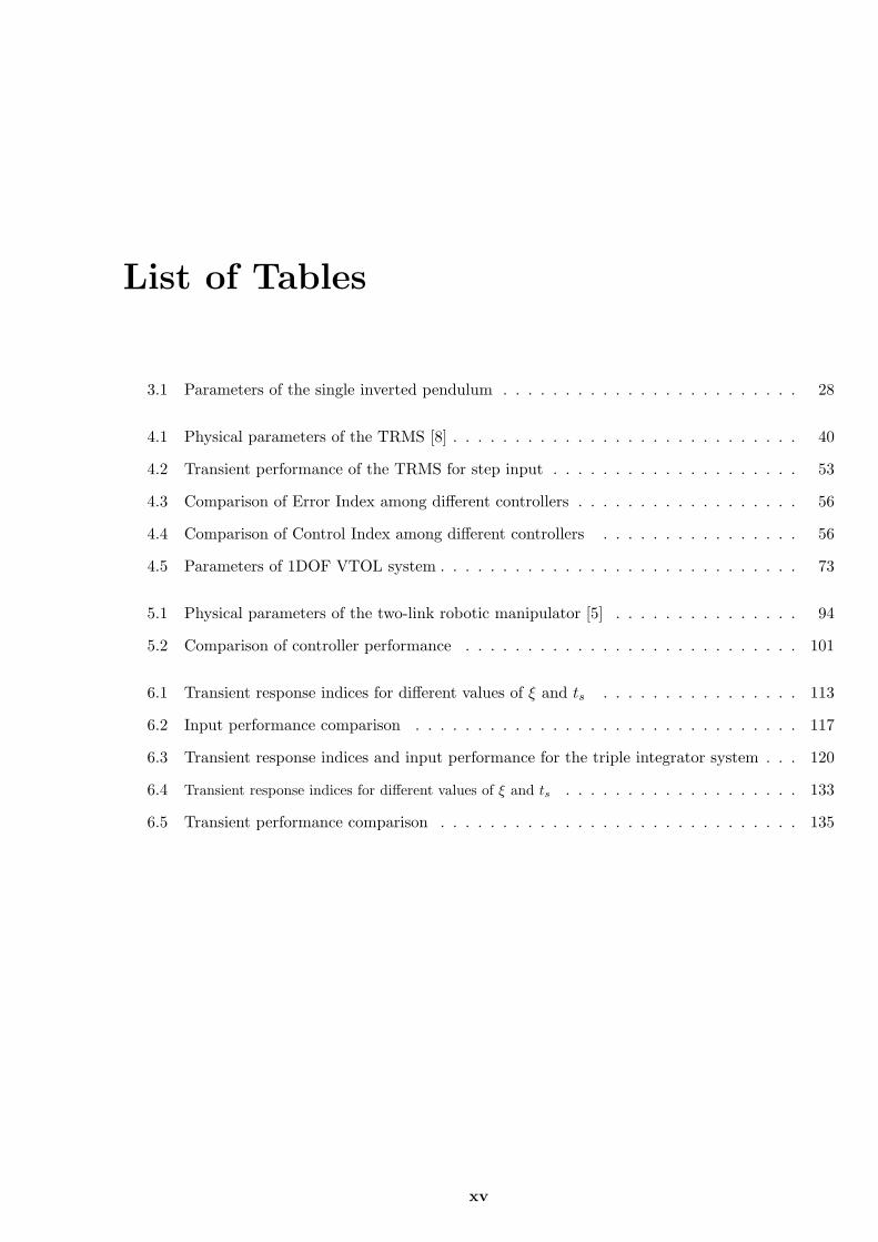
List of Tables
3.1 Parameters of the single inverted pendulum . . . . . . . . . . . . . . . . . . . . . . . . 28
4.1 Physical parameters of the TRMS [8] . . . . . . . . . . . . . . . . . . . . . . . . . . . . 40
4.2 Transient performance of the TRMS for step input . . . . . . . . . . . . . . . . . . . . 53
4.3 Comparison of Error Index among different controllers . . . . . . . . . . . . . . . . . . 56
4.4 Comparison of Control Index among different controllers . . . . . . . . . . . . . . . . 56
4.5 Parameters of 1DOF VTOL system . . . . . . . . . . . . . . . . . . . . . . . . . . . . . 73
5.1 Physical parameters of the two-link robotic manipulator [5] . . . . . . . . . . . . . . . 94
5.2 Comparison of controller performance . . . . . . . . . . . . . . . . . . . . . . . . . . . 101
6.1 Transient response indices for different values of ξ and ts . . . . . . . . . . . . . . . . 113
6.2 Input performance comparison . . . . . . . . . . . . . . . . . . . . . . . . . . . . . . . 117
6.3 Transient response indices and input performance for the triple integrator system . . . 120
6.4 Transient response indices for different values of ξ and ts . . . . . . . . . . . . . . . . . . . 133
6.5 Transient performance comparison . . . . . . . . . . . . . . . . . . . . . . . . . . . . . 135
xv
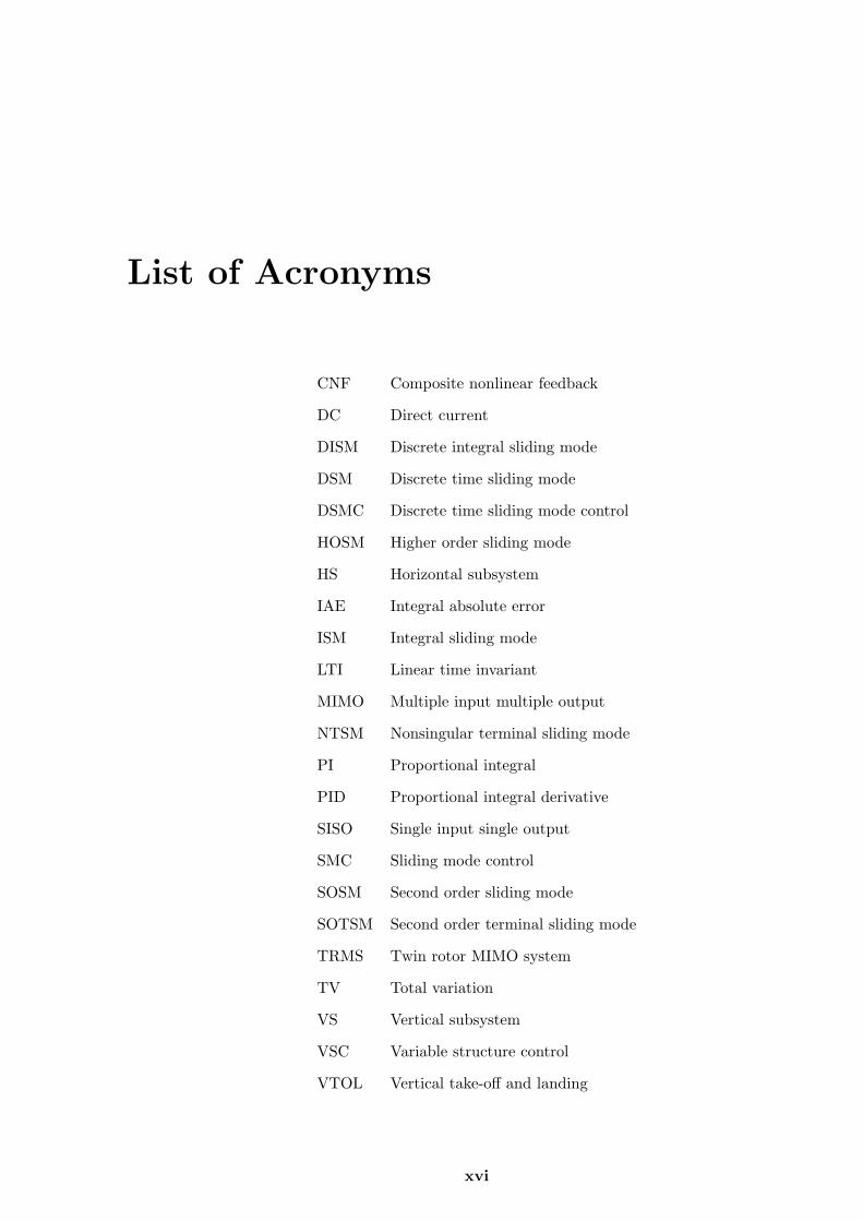
List of Acronyms
CNF Composite nonlinear feedback
DC Direct current
DISM Discrete integral sliding mode
DSM Discrete time sliding mode
DSMC Discrete time sliding mode control
HOSM Higher order sliding mode
HS Horizontal subsystem
IAE Integral absolute error
ISM Integral sliding mode
LTI Linear time invariant
MIMO Multiple input multiple output
NTSM Nonsingular terminal sliding mode
PI Proportional integral
PID Proportional integral derivative
SISO Single input single output
SMC Sliding mode control
SOSM Second order sliding mode
SOTSM Second order terminal sliding mode
TRMS Twin rotor MIMO system
TV Total variation
VS Vertical subsystem
VSC Variable structure control
VTOL Vertical take-off and landing
xvi
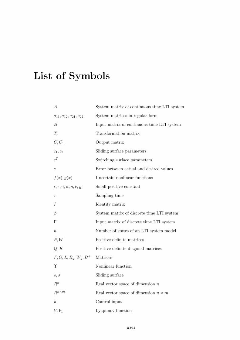
List of Symbols
A System matrix of continuous time LTI system
a11, a12, a21, a22 System matrices in regular form
B Input matrix of continuous time LTI system
Tr Transformation matrix
C,C1 Output matrix
c1, c2 Sliding surface parameters
cT Switching surface parameters
e Error between actual and desired values
f(x), g(x) Uncertain nonlinear functions
ϵ, ε, γ, κ, η, ν, ϱ Small positive constant
τ Sampling time
I Identity matrix
ϕ System matrix of discrete time LTI system
Γ Input matrix of discrete time LTI system
n Number of states of an LTI system model
P,W Positive definite matrices
Q,K Positive definite diagonal matrices
F,G,L,Bg,Wg, B+ Matrices
Υ Nonlinear function
s, σ Sliding surface
Rn Real vector space of dimension n
Rn×m Real vector space of dimension n×m
u Control input
V, V1 Lyapunov function
xvii
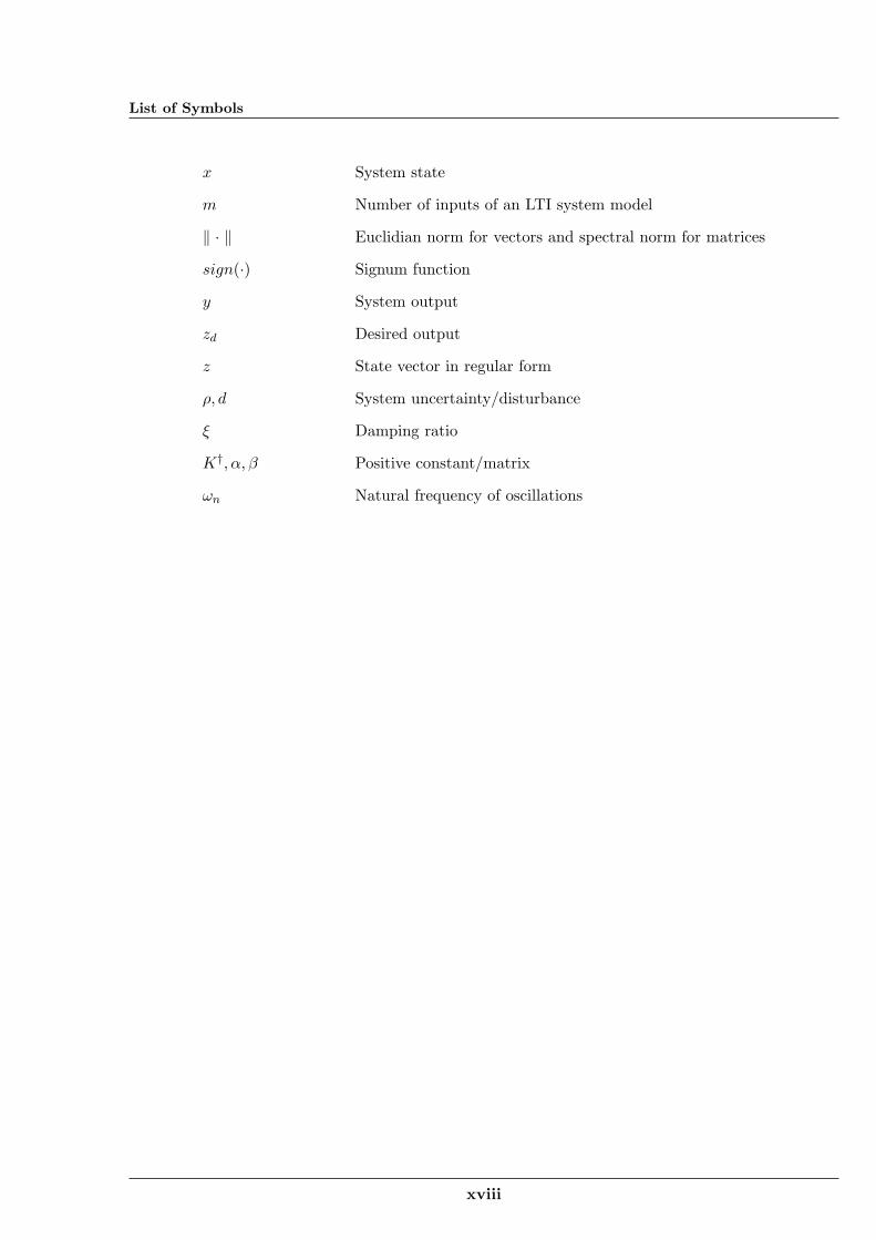
List of Symbols
x System state
m Number of inputs of an LTI system model
∥ · ∥ Euclidian norm for vectors and spectral norm for matrices
sign(·) Signum function
y System output
zd Desired output
z State vector in regular form
ρ, d System uncertainty/disturbance
ξ Damping ratio
K†, α, β Positive constant/matrix
ωn Natural frequency of oscillations
xviii
List of Publications
Refereed Journals
1. S. Mondal and C. Mahanta, “Adaptive Second order Terminal Sliding Mode Controller for
Robotic Manipulators”, Journal of the Franklin Institute, Elsevier, Accepted.
2. S. Mondal and C. Mahanta, “Chattering Free Adaptive Multivariable Sliding Mode Controller
for Systems with Matched and Mismatched Uncertainty”, ISA Transactions, Elsevier, 52(3), pp.
335-341, 2013.
3. S. Mondal and C. Mahanta, “Adaptive Integral Higher Order Sliding Mode Controller for Un-
certain Systems”, Journal of Control Theory Applications, Springer, 11(1), pp. 61-68, 2013.
4. S. Mondal and C. Mahanta, “Adaptive second-order sliding mode controller for a twin rotor
multi-input-multi-output system”, IET Control Theory & Applications, vol. 6(14), pp. 2157-
2167, 2012.
5. S. Mondal and C. Mahanta, “A Fast Converging Robust Controller using Adaptive Second Order
Sliding Mode”, ISA Transactions, Elsevier, vol. 51(6), pp. 713-721, 2012.
6. S. Mondal and C. Mahanta, “Composite Nonlinear Feedback based Discrete Integral Sliding
Mode Controller for Uncertain Systems”, Communications in Nonlinear Science and Numerical
Simulation, Elsevier, vol. 17(3), pp. 1320-1331, 2012.
7. S. Mondal and C. Mahanta, “Nonlinear Sliding Surface based Second Order Sliding Mode Con-
troller for Uncertain Linear Systems”, Communications in Nonlinear Science and Numerical
Simulation, Elsevier, vol. 16(9), pp. 3760-3769, 2011.
xix
List of Publications
Conference Proceedings
1. S. Mondal, and C. Mahanta, “Observer based Sliding Mode Control Strategy for Vertical Take-
Off and Landing (VTOL) Aircraft System”, 8th IEEE Conference on Industrial Electronics and
Applications (ICIEA),pp. 1-5, 19-21th June, 2013, Melbourne, Australia.
2. S. Mondal, T.V. Gokul and C. Mahanta, “Adaptive Second Order Sliding Mode Controller for
Vertical Take-off and Landing Aircraft System”, 6th International Conference on Industrial and
Information Systems (ICIIS),pp. 1-5, 6-9th August, 2012, IITMadras, India.
3. S. Mondal, T.V. Gokul and C. Mahanta, “Chattering Free Sliding Mode Controller for Mis-
matched Uncertain System”, 6th International Conference on Industrial and Information Sys-
tems (ICIIS),pp. 1-5, 6-9th August, 2012, IITMadras, India.
4. S. Mondal and C. Mahanta, “Improved Adaptive Control of Nonlinear Uncertain Systems
Through Second Order Sliding Mode Controller”, Proc. 12th IEEE Workshop on Variable Struc-
ture Systems, pp. 100-104, 12-14th January, 2012, Mumbai, India.
5. S. Mondal and C. Mahanta, “Second Order Sliding Mode Controller for Twin Rotor MIMO
System”, Proc. INDICON 2011, pp. 1-5, 17-18th December, 2011, Hyderabad, India.
6. S. Mondal and C. Mahanta,“Controlling Uncertain Systems with Variable Gain based Second
Order Integral Sliding Mode Controller”, Proc. National System Conference 2011 (NSC 2011),
9-11th December, 2011, Bhubaneswar, India.
7. S. Mondal and C. Mahanta, “Nonlinear Feedback Based Discrete Integral Sliding Mode Con-
troller for Linear Uncertain System”, Proc. National System Conference 2010 (NSC 2010),
10-12th December, 2010, Surathkal, India.
8. S. Mondal and C. Mahanta, “Discrete-time Sliding Mode Tracking Control for Uncertain Sys-
tems”, Proc. 4th International Conference on Computer Applications in Electrical Engineering
Recent Advances, 19-21 February, 2010, IIT Roorkee, India.
xx

1Introduction
Contents
1.1 Introduction . . . . . . . . . . . . . . . . . . . . . . . . . . . . . . . . . . . . 2
1.2 Motivation and purpose . . . . . . . . . . . . . . . . . . . . . . . . . . . . . 3
1.3 Contributions of this Thesis . . . . . . . . . . . . . . . . . . . . . . . . . . . 5
1.4 Organization of the Thesis . . . . . . . . . . . . . . . . . . . . . . . . . . . . 5
1
1. Introduction
1.1 Introduction
In reality, all physical systems are affected by uncertainties occurring due to modeling error, para-
metric variation and external disturbance. Controlling dynamical systems in presence of uncertainties
is extremely difficult as performance of the controller degrades and the system may even be driven to
instability. As such, active research is continuing to develop controllers which can work successfully
in spite of uncertainties. Robust control techniques such as nonlinear adaptive control [9], model
predictive control [10], backstepping [11] and sliding mode control [12, 13] have evolved to deal with
uncertainties. These control techniques are capable of achieving the specified control objectives in
spite of modeling errors and parametric uncertainties affecting the controlled system. Beginning in
the late 1970s and continuing till today, the sliding mode control (SMC) [14, 15] methodology has
received wide attention because of its inherent insensitivity to parametric variations and external dis-
turbances. The sliding mode control (SMC) is a particular type of variable structure control system
(VSCS) which uses a discontinuous control input. Recently many successful practical applications of
sliding mode control (SMC) have established the importance of sliding mode theory. Sliding mode
controllers are now-a-days widely used in a variety of application areas like robotics, process control,
aerospace and power electronics [16, 17]. The research in this held was initiated by Emel’yanov and
his colleagues [14] and the design paradigm now forms a mature and established approach for robust
control and estimation. The idea of sliding mode control (SMC) was not known to the control com-
munity at large until an article published by Utkin [15] and a book by Itkis [18].
Design of the SMC involves two key steps, viz. (1) the design of a sliding surface in accordance with
the desired closed loop performance and (2) the design of a suitable control law. The sliding surface is
to be designed optimally to satisfy all constraints and required specifications. The initial phase when
the state trajectory is directed towards the sliding surface is called the reaching phase. During the
reaching phase, the system is sensitive to all types of disturbances. However, a control law can be
designed which ensures finite time reaching of the sliding surface even in the presence of uncertain-
ties and disturbances. For eliminating the non-robust reaching phase, an integral sliding mode was
proposed in [19, 20] which naturally allowed SMC to be combined with other techniques. The main
advantages of the SMC are the following:
(i) During the sliding mode, the system is insensitive to matched model uncertainties and distur-
bances [21].
2
1.2 Motivation and purpose
(ii) When the system is on the sliding manifold, it behaves as a reduced order system with respect to
the original plant.
However, in spite of the claimed robustness, implementation of the SMC in real time is handicapped by
a major drawback known as chattering which is the high frequency bang-bang type of control action.
Chattering is caused due to the fast dynamics which are usually neglected in the ideal model of sliding
mode. In the ideal sliding mode, the control is assumed to switch with an infinite frequency. However,
in actual plants, due to the inertia of actuators and sensors as well as the presence of nonlinearities, the
switching occurs with high but finite frequency only. The main consequence is that the sliding mode
takes place in a small neighborhood of the sliding manifold, whose dimension is inversely proportional
to the control switching frequency. In sliding mode, due to the finite switching of control signal, the
states would switch about the sliding surface rather than lie directly on it. This switching can occur
at a high frequency and is called chattering. The effect of chattering is that the high frequency com-
ponents of the control propagate through the system and thereby excite the unmodeled fast dynamics
and give rise to undesired oscillations which affect the system output. This can degrade the system
performance or may even lead to instability. Moreover, the term chattering has been designated to
indicate the bad effect, potentially disruptive, that a switching control can produce on a controlled
mechanical plant. Chattering as well as the necessity of discontinuous control are two main criticisms
against practical realization of sliding mode control scheme. These drawbacks are more prominent
while dealing with mechanical systems since rapidly changing control actions induce stress and wear
in mechanical parts and the system may even suffer breakdown in a short time [22].
1.2 Motivation and purpose
In order to overcome the above mentioned drawbacks, efforts are on to find a continuous control
action which is robust against uncertainties and guarantees the same control objective as offered by the
standard sliding mode approach. Different approaches have been proposed to avoid chattering [21,23].
The main idea of such approaches was to change the dynamics in a small vicinity of the discontinuity
surface in order to avoid real discontinuity and, at the same time, to preserve the main properties
of the whole system. However, the ultimate accuracy and robustness of the sliding mode are par-
tially lost in this process. The commonly used approach is by using continuous approximations of the
sign(·) function (such as the sat(·) function, the tanh(·) function) in the implementation of the control
3
1. Introduction
law. An interesting approach evolved for elimination of chattering was the higher order sliding mode
methodology introduced by Arie Levant [24–26]. The higher order sliding modes generalize the basic
sliding mode idea by acting directly on the higher order time derivatives of the sliding variable instead
of influencing its first time derivative only as it happens in standard sliding modes. Keeping the
main advantages of the original approach, higher order sliding modes remove the chattering effect and
provide even higher accuracy. A number of higher order sliding mode controllers are proposed in the
literature [12, 25–29]. However, the main constraint in implementation of higher order sliding modes
is the increasing information demand. In general, any r-th order sliding mode controller requires the
knowledge of the time derivatives of the sliding variable up to the (r-1)-th order. The only exceptions
are provided by the twisting controller [24], the super twisting controller [24] and the sub-optimal
algorithm. Among higher order sliding mode controllers, second order sliding mode controllers are
the most widely used because of their simplicity and low information demand. In second order sliding
mode methodology, the control action affects directly the sign and the amplitude of the sliding vari-
able and a suitable switching logic guarantees the finite time convergence of the state to the sliding
manifold.
Sliding mode control [30] has been extensively used in control systems perturbed by matched uncer-
tainty which enters the system through the input channel. However, designing sliding mode controllers
for systems perturbed by the mismatched type of uncertainty, which is due to perturbations in the
system parameters, still remains a challenge to the research community. The difficulty lies in the fact
that the dynamics of the uncertain system are affected even after reaching the sliding mode. Active
research is continuing in the control community for developing sliding mode controllers for systems
affected by mismatched type of uncertainty. By designing a sliding mode controller for certain states
of the system which are provided as inputs to a reduced order system can take care of mismatched
uncertainties. However, the disadvantage of this method is that uncertainties should lie in the range
space of certain matrix of the nominal system [30]. A fuzzy logic based sliding mode controller pro-
posed in [31] was successful in achieving quadratic stability for systems with mismatched uncertainty.
Even this method could handle mismatched uncertainty of a certain form only provided its bound was
known apriori [32, 33]. By introducing two sets of switching surfaces for the subsystems and hence
reducing the rank of the uncertainty, asymptotic stability was achieved in [34]. Dynamic output feed-
back sliding mode controllers were attempted in [35] and nonlinear integral type sliding surface was
4
1.3 Contributions of this Thesis
used to deal with mismatched uncertainties in [36]. All these works required prior knowledge about
the upper bound of the mismatched uncertainty which was in general difficult to obtain. Hence a
strategy to obtain the upper bound of the system uncertainty or a method which does not require this
knowledge is needed. The adaptive sliding mode controller proposed by Cheng at al. [3,37,38] provided
a solution to this problem. However, this adaptive method yielded gains which were overestimated in
many cases giving rise to large control efforts and high chattering [39,40].
Motivated by the above reasons, this thesis attempts to develop suitable sliding mode control strate-
gies which can eliminate chattering. In particular, this thesis aims for designing chattering free sliding
mode controllers which can effectively handle systems with uncertainties of both matched and mis-
matched type, without requiring the prior knowledge about the upper bound of the uncertainty. The
effectiveness of the developed sliding mode control scheme is validated by applying the controller to
important benchmark control problems like the twin rotor MIMO system (TRMS), the vertical take-
off and landing system (VTOL) and the two-link robotic manipulator which are typical examples of
highly nonlinear systems affected by severe uncertainties.
1.3 Contributions of this Thesis
The main contribution of this thesis is the design of a chattering free adaptive sliding mode
controller for systems affected by both matched and mismatched types of uncertainty. The control
law is designed in such a way that the discontinuous sign function acts on the time derivative of the
control input. So the actual control obtained after integration is continuous and hence chattering
is eliminated. Adaptive tuning mechanism is used to estimate the upper bound of the uncertainty,
thereby eliminating the necessity of its prior knowledge. The proposed idea of adaptive chattering
free sliding mode is used to design integral and terminal sliding mode controllers. A nonlinear sliding
surface based adaptive sliding mode controller is proposed for improving transient performances like
overshoot and settling time.
1.4 Organization of the Thesis
This thesis is divided into seven chapters. A brief description about each chapter is presented in
this section.
5
1. Introduction
• Chapter 2: A few preliminary and basic concepts related to sliding mode control are discussed
in Chapter 2.
• Chapter 3: In this chapter a chattering free adaptive integral sliding mode controller for
uncertain systems is proposed. Instead of a regular control input, the derivative of the control
input is used in the proposed control law. The discontinuous sign function in the controller is
made to act on the time derivative of the control input. The actual control signal obtained by
integrating the derivative control signal is smooth and chattering free. The adaptive tuning law
used in the proposed controller eliminates the need of prior knowledge about the upper bound
of the system uncertainty.
• Chapter 4: In this chapter an adaptive sliding mode controller for coupled multi input multi
output (MIMO) systems affected by both matched and mismatched uncertainties is proposed.
More specifically, the problem of controlling a twin rotor MIMO system (TRMS) in cross-coupled
condition is addressed using adaptive sliding mode control technique. An adaptive mechanism
is embedded in the controller as well as the sliding surface to overcome the perturbations.
The proposed controller with adaptive sliding surface is implemented for a vertical take-off and
landing (VTOL) aircraft system affected by matched and mismatched uncertainties. An adaptive
gain tuning mechanism is used to ensure that the gain is not overestimated with respect to the
actual unknown value of the uncertainty. A case study was conducted on the laboratory set-up
of a 1 degree of freedom VTOL system to investigate the real time performance of the proposed
adaptive sliding mode controller.
• Chapter 5: In this chapter an adaptive chattering free terminal sliding mode controller is
proposed to ensure fast and finite time stabilization of uncertain systems. Instead of the normal
control input, its time derivative is used in the proposed controller. An adaptive tuning method
is utilized to deal with the system uncertainties whose upper bounds are not required to be
known in advance.
• Chapter 6: An adaptive sliding mode controller is proposed in this chapter using nonlinear slid-
ing surface which ensures better transient performance over linear sliding surfaces. One major
benefit is that chattering is completely removed from the control signal. To improve the perfor-
mance of discrete time uncertain systems, an algorithm based on integral sliding mode (ISM)
6
1.4 Organization of the Thesis
and composite nonlinear feedback (CNF) is proposed. The discrete CNF based ISM method
ensures fast rise time and less overshoot as compared to ISM method with linear feedback.
• Chapter 7: In this chapter conclusions from the research work are drawn and the scope for
future research is outlined.
7
2Preliminary Concepts
Contents
2.1 Introduction . . . . . . . . . . . . . . . . . . . . . . . . . . . . . . . . . . . . 9
2.2 Variable Structure System and Sliding Mode . . . . . . . . . . . . . . . . . 9
2.3 Stability of the Sliding mode . . . . . . . . . . . . . . . . . . . . . . . . . . 11
2.4 Relative Degree in Sliding Mode . . . . . . . . . . . . . . . . . . . . . . . . 12
2.5 Order of the sliding mode . . . . . . . . . . . . . . . . . . . . . . . . . . . . 12
2.6 Finite time stability . . . . . . . . . . . . . . . . . . . . . . . . . . . . . . . . 13
2.7 Chattering . . . . . . . . . . . . . . . . . . . . . . . . . . . . . . . . . . . . . . 15
2.8 Summary . . . . . . . . . . . . . . . . . . . . . . . . . . . . . . . . . . . . . . 17
8
2.1 Introduction
2.1 Introduction
In this chapter, preliminary concepts relevant to sliding mode control are discussed briefly. The
necessary fundamentals of the sliding mode are explained concisely so that the sliding mode con-
troller design and analysis carried out in the succeeding chapters can be easily followed. Chattering
phenomenon which is an undesired phenomenon occurring in conventional sliding mode controller is
explained and methods devised for chattering mitigation are introduced. Finite time stability which
is an important notion in sliding mode control is described. First and second order sliding modes are
explained to highlight the basic difference between the two.
2.2 Variable Structure System and Sliding Mode
A variable structure system (VSS) [15] is a dynamical system whose structure changes according
to an appropriate switching logic in order to exploit the desirable properties of these structures. To
illustrate, let us consider the following dynamical system
x = f(t, x, u) (2.1)
where x ∈ Rn are the state variables and u ∈ Rm is the control input.
Further,
u = [u1(t, x), u2(t, x), ..., um(t, x)]T (2.2)
where
ui =
u+i (t, x), if σi(x) > 0
u−i (t, x), if σi(x) < 0
i = 1, 2, ...m
(2.3)
Here
σ(x) = [σ1(x) σ2(x)....σm(x)]T (2.4)
is the sliding manifold and σi(x) = 0(i = 1, 2, ...m) is the i-th sliding surface. The motion on the
sliding manifold σ(x) = 0 is called the sliding mode.
The differential equation (2.1) does not formally satisfy the classical theorem on the existence and
9
2. Preliminary Concepts
uniqueness of the solution since it has discontinuous right hand side. Moreover, the right hand side
is usually not defined on the discontinuity surfaces. Thus, it fails to satisfy conventional existence
and uniqueness results of differential equation theory. Nevertheless, an important aspect of sliding
mode control design is the assumption that the system state behaves in a unique way when restricted
to σ(x) = 0. Therefore, the problem of existence and uniqueness of differential equations with dis-
continuous right hand sides is of fundamental importance. Various types of existence and uniqueness
theorems are proposed by Utkin [15], Itkis [18], Hajeck [41] and Filippov [42]. The method of Filip-
pov [42] is conceptually straightforward. This method is now briefly recalled to help in understanding
variable structure system behaviour on the switching surface.
Let us now consider an n-th order VSS system with a single input as given below,
x = f(t, x, u) (2.5)
with the following general control strategy
u =
u+(t, x), if σ(x) > 0
u−(t, x), if σ(x) < 0(2.6)
The system dynamics are not directly defined on the manifold σ(x) = 0. It has been shown by Fil-
ippov that the state trajectories of (2.5) with control (2.6) on σ(x) = 0 are the solutions of the equation
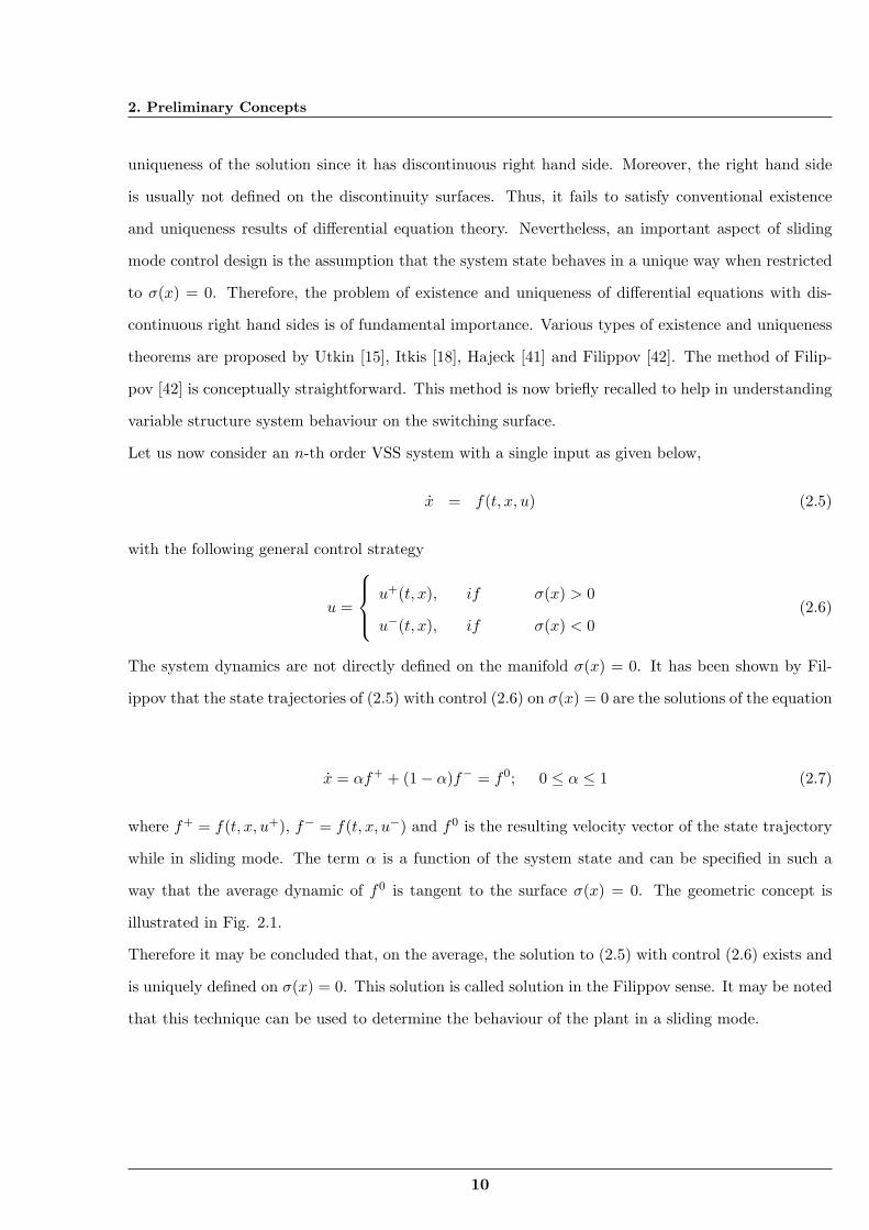
x = αf+ + (1 − α)f− = f0; 0 ≤ α ≤ 1 (2.7)
where f+ = f(t, x, u+), f− = f(t, x, u−) and f0 is the resulting velocity vector of the state trajectory
while in sliding mode. The term α is a function of the system state and can be specified in such a
way that the average dynamic of f0 is tangent to the surface σ(x) = 0. The geometric concept is
illustrated in Fig. 2.1.
Therefore it may be concluded that, on the average, the solution to (2.5) with control (2.6) exists and
is uniquely defined on σ(x) = 0. This solution is called solution in the Filippov sense. It may be noted
that this technique can be used to determine the behaviour of the plant in a sliding mode.
10
2.3 Stability of the Sliding mode
!(x)=0 !
"
#
Figure 2.1: Illustration of Filippov method
2.3 Stability of the Sliding mode
The objective of sliding mode control is to ensure sliding motion in finite time from an arbitrary
initial condition. The system state must approach the sliding surface at least asymptotically. The
largest such neighborhood is called the region of attraction. Stability of the sliding surface requires
to choose a generalized Lyapunov function V (t, x) which is positive definite and has a negative time
derivative in the region of attraction. Unfortunately, there are no standard methods to find Lyapunov
functions for arbitrary nonlinear systems.
For all single input systems, a suitable Lyapunov function can be chosen as
V (t, x) =12σ2(x) (2.8)
which clearly is globally positive definite.
If
V (t, x) = σ(x)σ(x) < 0 (2.9)
in the domain of attraction, then the state trajectory converges to the sliding surface and is restricted
to the surface for all subsequent time. This latter condition is called the reaching or reachability
condition [12] [22] [30] [43] and it ensures that the sliding manifold is reached asymptotically.
11
2. Preliminary Concepts
A strong condition for finite time reaching is given as follows
V (t, x) = σ(x)σ(x) ≤ −η|σ(x)| (2.10)
for some η > 0, known as η reachability condition in the literature. For a general m input system, it
is not necessary to ensure sliding mode on each discontinuity surface but sliding mode should exist on
the intersection of all discontinuity surfaces. These conditions ascertain that sliding surfaces remain
attractive.
2.4 Relative Degree in Sliding Mode
Definition 2.1. A smooth autonomous single input single output (SISO) system x = a(t, x) +
b(t, x)u with the control u and output σ is said to have the relative degree r, if the Lie derivatives
locally satisfy the conditions [44]
Lbσ = LaLbσ = .... = Lr−2a Lbσ = 0, Lr−1
a Lbσ = 0. (2.11)
It can be shown that the equality of the relative degree to r actually means that σ, σ, ..., σ(r−1) do
not depend on control and can be taken as a part of new local coordinates and σ(r) linearly depends
on u with the nonzero coefficient Lr−1a Lbσ.
2.5 Order of the sliding mode
The standard sliding mode can be implemented only if the relative degree of the sliding variable
is 1, i.e. control has to appear in its first total time derivative σ. Another problem of the standard
sliding mode is that the high frequency switching in the control may cause dangerous vibrations called
chattering. The sliding mode order approach [24] addresses both these issues of relative degree restric-
tion and chattering while preserving the features of the sliding mode. The sliding order characterizes
the dynamics smoothness degree in the vicinity of the sliding mode and can be defined as given below:
Definition 2.2. Let us consider a discontinuous differential equation x = f(t, x) understood in
the Filippov sense [42] and σ(x) is a smooth function. Then, provided that
1. σ, σ, ..., σ(r−1) are continuous functions of x,
12
2.6 Finite time stability
2. the set
σ = σ = σ = ......... = σ(r−1) = 0 (2.12)
is a non-empty integral set,
the motion on set (2.12) is said to exist in r-sliding (rth-order sliding) mode [24] [45]. The set
(2.12) is called r-sliding set. It is said that the sliding order is strictly r, if the next derivative σ(r) is
discontinuous or does not exist as a single-valued function of x.
2.6 Finite time stability
The standard sliding mode used in the traditional VSSs is of the first order (σ is continuous and σ
is discontinuous). The standard sliding mode design suggests choosing a new auxiliary sliding variable
of the first relative degree. That variable is usually a linear combination of the sliding variable σ and
its successive total time derivatives [23], which leads to only exponential stabilization of σ. The finite
time stabilization corresponds to the high order sliding mode (HOSM) approach [24] [27]. Asymptoti-
cally stable HOSMs arise in systems with traditional sliding mode control, if the relative degree of the
sliding variable σ is higher than 1. An important property which concerns asymptotic stability is finite
time stability (FTS), i.e. the solutions of a system which reach the equilibrium point in finite time.
Finite time stability is preferable, since it offers higher robustness and higher accuracy in presence
of small sampling noises and delays. The concept of finite time stability corresponding to high order
sliding mode (HOSM) is explicitly discussed in [46] [47] [48] [49] [50] [51]. A simple definition of finite
time stability as given in [47] is stated below:
The main idea of finite time stability lies in assigning infinite eigenvalue to the closed loop system
at the origin and therefore the right hand side of the ordinary differential equation can not be locally
Lipschitz at the origin. Also there exists the settling time function T (x0) where x0 is the initial
condition that determines time for a solution to reach the equilibrium. This settling time function (in
general) depends on the initial condition of a solution.
13
2. Preliminary Concepts
Let us consider the following example [49] [50] [51]
x = −|x|asgn(x) x ∈ Rn, (2.13)
for which the solutions are (a ∈]0, 1[):
x(t, x0) =
s(t, x0), if 0 ≤ t ≤ |x0|1−a
1−a
0, if t > |x0|1−a
1−a
(2.14)
with s(t, x0) = sgn(x0)(|x0|1−a − t(1 − a))1
1−a and they reach the origin in finite time. The time
required for the solutions to reach the equilibrium is called the settling time which depends on the
initial condition of the solution.
Definition 2.3. Finite time stability of continuous autonomous systems [49] [50] [51]
Let us consider the continuous autonomous system
x = f(x), x ∈ Rn (2.15)
The origin of the system (2.15) is finite time stable (on an open neighbourhood V ⊂ Rn) if [52]:
• there exits a function T : V \ 0 → R≥0 such that if x0 ∈ V \ 0 then Φx0(t) is defined (and in
particular is unique) on [0, T (x0)), Φx0(t) ∈ V \ 0 for all t ∈ [0, T (x0)) and limt→T (x0)
Φx0(t) = 0.
The quantity T is called settling time function of system (2.15).
• for all ϵ > 0, there exists a function δ(ϵ) > 0, for every x0 ∈ (δ(ϵ)Bn \ 0)∩
V, Φx0(t) ∈ ϵBn
for all t ∈ [0, T (x0))
where B is the unit open ball in Rn and Φx0(t) denotes a solution of system (2.15) starting from
x0 ∈ Rn at t = 0.
Definition 2.4. Finite time stability of discontinuous systems [52]
Let us consider the differential inclusion
x ∈ F (x), x ∈ Rn (2.16)
where F is a set valued function on Rn, x denotes the right derivative of x. The origin of (2.16)
is finite time stable if
14
2.7 Chattering
• the origin of the system (2.16) is stable : if for all ϵ > 0, there is δ(ϵ) > 0 such that if x0 ∈ δ(ϵ)B,
then any solution ϕx0 starting at x0 is defined for all t ≥ 0 and ϕx0(t) ∈ ϵB for all t ≥ 0,
• there exists T0 : S → R≥0, such that for all solutions ϕx0 ∈ S(x0), ϕx0(t) = 0 for all t ≥ T0(ϕx0).
T0 is the settling time of the solution ϕx0 .
Here ϕx0(t) represents a solution of system (2.16) starting from x0, S(x0) is the set of all solutions ϕx0
and space S =∪
x0∈Rn
S(x0).
If T (x) = supϕx∈S(x)
T0(ϕx) < +∞, then T (x) is the time for the solution ϕx to reach the origin called
the settling time function of system (2.16).
2.7 Chattering
In real life applications, it is not reasonable to assume that the control signal can switch at infinite
frequency. Due to the presence of inertia in actuators and sensors, surrounding noise and exogenous
disturbances, actually the control signal commutes at a very high though finite frequency. The control
signal’s oscillation frequency turns out to be not only finite but also almost unpredictable. Its main
consequence is that the sliding mode takes place in a small neighbourhood of the sliding manifold
whose width is inversely proportional to the control switching frequency [12] [22] [30].
The notions of ideal and real sliding mode are adopted here to distinguish the sliding motion that
occurs ideally on the sliding manifold (assuming ideal control devices) from a sliding motion that,
due to the non-idealities of the control law implementation, takes place in a vicinity of the sliding
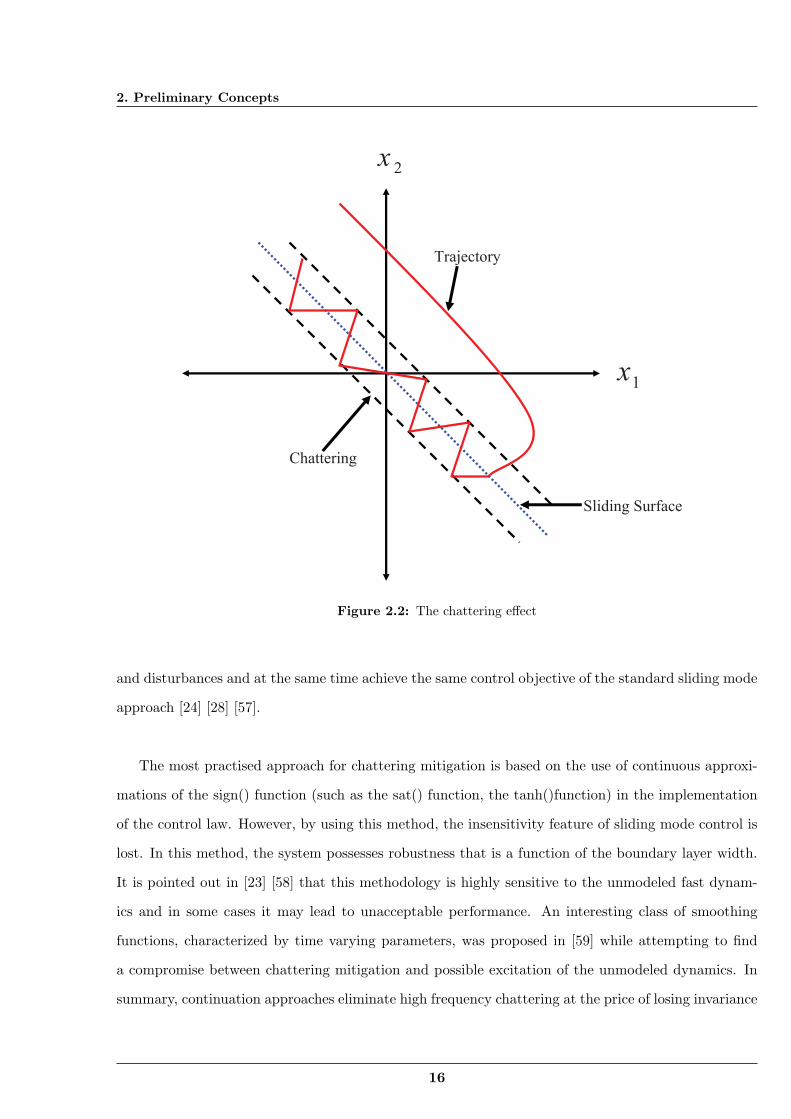
manifold, which is called the boundary layer (illustrated in Fig. 2.2).
The effect of the finite switching frequency of the control is referred in the literature as chatter-
ing [53] [54] [55]. Basically, the high frequency components of the control propagate through the
system, thereby exciting the unmodeled fast dynamics resulting in undesired oscillations which affect
the system output. This phenomenon degrades the system performance or may even lead to insta-
bility. The term chattering has also been designated to indicate the potentially disruptive affect that
a switching control force or torque can produce on a controlled mechanical plant [23] [27] [55] [56].
Chattering and high control activity are the major drawbacks of the sliding mode approach in the
practical realization of sliding mode control schemes. Active research is continuing to realize a contin-
uous control action which can overcome these drawbacks and ensure robustness against uncertainties
15
2. Preliminary Concepts
2x
1x
Trajectory
Sliding Surface
Chattering
Figure 2.2: The chattering effect
and disturbances and at the same time achieve the same control objective of the standard sliding mode
approach [24] [28] [57].
The most practised approach for chattering mitigation is based on the use of continuous approxi-
mations of the sign() function (such as the sat() function, the tanh()function) in the implementation
of the control law. However, by using this method, the insensitivity feature of sliding mode control is
lost. In this method, the system possesses robustness that is a function of the boundary layer width.
It is pointed out in [23] [58] that this methodology is highly sensitive to the unmodeled fast dynam-
ics and in some cases it may lead to unacceptable performance. An interesting class of smoothing
functions, characterized by time varying parameters, was proposed in [59] while attempting to find
a compromise between chattering mitigation and possible excitation of the unmodeled dynamics. In
summary, continuation approaches eliminate high frequency chattering at the price of losing invariance
16
2.8 Summary
towards uncertainty. One effective approach for chattering elimination is by using the second order
sliding mode methodology [24] [27].
2.8 Summary
In this chapter, basic concepts and properties of sliding modes have been discussed concisely. The
main advantages of the sliding mode control technique are the simplicity in both implementation and
design and the inherent robustness with respect to matched internal and external uncertainties and
disturbances.
17
3Adaptive Integral Sliding Mode
Controller
Contents
3.1 Introduction . . . . . . . . . . . . . . . . . . . . . . . . . . . . . . . . . . . . 19
3.2 Problem Definition . . . . . . . . . . . . . . . . . . . . . . . . . . . . . . . . 20
3.3 Design of adaptive integral sliding mode controller . . . . . . . . . . . . . 21
3.4 Simulation Examples . . . . . . . . . . . . . . . . . . . . . . . . . . . . . . . 26
3.5 Summary . . . . . . . . . . . . . . . . . . . . . . . . . . . . . . . . . . . . . . 29
18
3.1 Introduction
3.1 Introduction
Sliding mode control (SMC), developed from the variable structure system theory, has gained
much more attention for its robustness against parameter variations and external disturbances under
matching conditions [30, 43, 60]. In sliding mode control (SMC), the system states are moved from
their initial states towards a chosen manifold in the state space, called the sliding surface [30, 43].
After reaching the sliding manifold, the system becomes totally insensitive to parametric uncertainties
and external disturbances. The motion of the trajectory from the initial condition towards the sliding
surface until it hits the sliding surface is called the reaching phase. During the reaching phase, the
system is not robust and even matched uncertainty can affect the system performance. To solve this
problem, an integral sliding mode (ISM) concept was proposed in [19].
In integral sliding mode control method, an integral term was incorporated in the sliding manifold
which guaranteed that the system trajectories would start in the manifold itself from the initial time
and thus the reaching phase was totally eliminated. Hence the system became invariant towards the
matching uncertainty right from the beginning.
Although the ISM controller guarantees robustness against system uncertainty, the crucial part is the
control discontinuity leading to chattering as explained in Chapter 2. Another difficulty faced by the
ISM controller is the necessity of prior knowledge about the upper bound of the system uncertainty.
In real time application it is very difficult to get the upper bound of the uncertainty and often this
bound is overestimated yielding to excessive gain.
For circumventing the above difficulties, this chapter proposes an integral sliding surface based chat-
tering free sliding mode controller which uses an adaptive tuning law. The main attributes of the
proposed controller are robustness and smooth control signal. An adaptive tuning law is used for the
controller to estimate the unknown but bounded system uncertainties. As such the upper bounds of
the system uncertainties are not required to be known in advance. Moreover, the chattering in the
control input is eliminated by using the proposed controller.
The brief outline of this chapter is as follows. Section 3.2 briefly discusses the design problem and
the assumptions made. In Section 3.3, the proposed adaptive integral sliding mode control method is
described. Section 3.4 presents simulation examples to demonstrate the efficiency and advantages of
the proposed controller. A brief summary of the chapter is presented in Section 3.5.
19
3. Adaptive Integral Sliding Mode Controller
3.2 Problem Definition
A class of nonlinear dynamic system is considered as follows:
x = f(x) + g(x)u
y = σ(x) (3.1)
where x ∈ Rn are the state variables, u ∈ R is the control input and σ(x) ∈ R is the measured output
function known as the sliding variable. It is assumed that f(x) and g(x) are smooth functions.
Let the system have a relative degree r with respect to the output variable σ which means that Lie
derivatives Lgσ;LfLgσ; ...;Lr−2f Lgσ are equal to zero identically in the vicinity of a given point and
Lr−1f Lgσ is not zero at the point. The equality of the relative degree to r means, in a simplified way,
that u first appears explicitly only in the r-th total time derivative of σ.
Remark 3.1 For simplicity, the relative degree of the system (3.1) is assumed to be equal to the order
of the sliding surface.
Assumption 3.1 The relative degree r of the system (3.1) is known a priori.
Assumption 3.2 An exact robust differentiator is available for exactly measuring or estimating the
derivative of variables.
The aim of the first order sliding mode control is to force the state trajectories to move along the
sliding manifold σ(x) = 0. In the higher order sliding mode control, the purpose is to move the
states along the switching surface σ(x) = 0 and to keep its (r − 1) successive time derivatives viz
σ, σ, ..., σ(r−1) to zero by using a suitable discontinuous control action [24]. The r-th order derivative
of σ(x) satisfies the following equation,
σ(r)(x) = a(x) + b(x)u (3.2)
where r is the relative degree, a(x) = Lrfσ(x) and b(x) = Lr−1f Lgσ(x). Here Lf and Lg are the Lie
derivatives [25] of the smooth functions in (3.1).
The r-th order sliding mode control of the system (3.1) with respect to the sliding variable σ(x) can
be expressed as [61],
zi = zi+1
zr = a(x) + b(x)u (3.3)
20
3.3 Design of adaptive integral sliding mode controller
where 1 ≤ i ≤ r − 1 and [z1, z2, ..., zr]T = [σ(x), σ(x), ..., σ(r−1)(x)]T
Assumption 3.3. Matrices a(x) and b(x) consist of the nominal parts (a(x), b(x)) which are known
apriori and uncertain parts (∆a(x), ∆b(x)) which are bounded and unknown [62].
Thus the following can be written,
a(x) = a(x) + ∆a(x)
b(x) = b(x) + ∆b(x) (3.4)
σ(r)(x) = (a+ ∆a)(x) + (b+ ∆b)(x)u
= a(x) + b(x)u+ ∆F (x, t) (3.5)
where ∆F (x, t) = ∆a(x) + ∆b(x)u includes all the uncertain parameters and external disturbance.
Using (3.4) and (3.5) with z as the state variable, the r-th order sliding mode control for the system
(3.1) can be written as,
zi = zi+1
zr = a(z) + b(z)u+ ∆F (z, t) (3.6)
In the regular form, the above can be written as,
z = A(z) + B(z)u+ ∆F (z, t) (3.7)
where z = [z1 z2...zi..zr]T , and A(z), B(z) are matrices with proper dimension. The uncertainties in
the system due to modeling error and parameter variation are denoted by ∆F (z, t) which is assumed
to be differentiable with respect to time. In this problem, the uncertainties in the system (3.6) are
assumed to meet the matching conditions. Then ∆F (z, t) ∈ spanB(z) [30] meaning that ∆F (z, t)
is a matched uncertainty.
3.3 Design of adaptive integral sliding mode controller
The design procedure for the overall control signal is carried out in two parts, design of the nominal
control wnom and then design of the overall control law u. At first, the nominal control law wnom is
designed that guarantees finite time stabilization of the chain of integrators in absence of uncertainties.
21
3. Adaptive Integral Sliding Mode Controller
Then the reaching law based overall control law is designed to reject the uncertainties and maintain
the sliding mode.
3.3.1 Finite time stabilization of an integrator chain system
Let us consider the nominal system which is represented by the single input single output (SISO)
integrator chain as described below,
z1 = z2
z2 = z3
.
zr = wnom (3.8)
The control objective is to drive the states of (3.8) to z = 0 at the fixed finite time [63].
Theorem 3.1. Let k1, k2, ...kn > 0 be such that the polynomial ϕ(λ) = λn + knλn−1 + ...+ k2λ+ k1
is Hurwitz. For the system (3.8), there exists a value ε ∈ (0, 1) such that for every αi ∈ (1 − ε, 1),
i = 1, 2, ...n, the origin is a globally stable equilibrium in finite time under the feedback
wnom(z) = −k1sign(z1)|z1|α1 − k2sign(z2)|z2|α2 − ...− knsign(zn)|zn|αn (3.9)
where α1, ...αn satisfy
αi−1 = αiαi+1
2αi+1−αi, i = 2, ..., n with αn+1 = 1 [63].
3.3.2 Design of integral sliding mode controller
However, when the system is perturbed or uncertain, the finite time stabilization is not ensured
[63]. In this section a reaching law based discontinuous control law is developed which rejects the
uncertainties of the system and ensures that the control objectives are fulfilled [62].
Let us consider an integral sliding surface,
s(z) = zn − zn(0) −∫wnom(z)dt (3.10)
The initial condition of the system is defined by zn(0). The nominal control wnom ensures the conver-
gence of the chain of integrators in finite time as given in Theorem 3.1.
22
3.3 Design of adaptive integral sliding mode controller
By taking the time derivative of (3.10), the following is obtained,
s(z) = zn − wnom
= a(z) + b(z)u+ ∆F (z, t) − wnom (3.11)
Using (3.11) and the constant rate reaching law s(z) = −Gsign(s(z)) [30] such that it satisfies the
reachability condition s(z)s(z) ≤ −η|s(z)| where η being a positive constant yields,
−Gsign(s(z)) = a(z) + b(z)u− wnom (3.12)
Here G is the switching gain. The control law described above ensures finite time stabilization of the
system states and also rejects the uncertainties if G > |∆F (z, t)|. Hence the overall control law can
be obtained as [62],
u = b(z)−1−a(z) + wnom −Gsign(s(z)) (3.13)
However, the high frequency chattering is always present in the control signal.
In order to remove the undesired chattering in the control input, an adaptive integral chattering free
sliding mode controller is developed. In the proposed controller, the time derivative of the control
input, u would be designed to act on the higher order derivatives of the sliding variable [64,65]. Hence
instead of the actual control u, the time derivative of the control, u would be used as the control
input. The new control v = u would be designed as a discontinuous signal, but its integral (the actual
control u) would be continuous thereby eliminating the high frequency chattering.
Now taking the first order time derivative of (3.11) yields,
s(z) = zn − wnom (3.14)
Using (3.2), (3.14) can be written as,
s(z) =d
dt(a(z) + b(z)u) − wnom
= ˙a(z) + ˙b(z)u+ b(z)u− wnom
= ˙a(z) + ˙b(z)u+ b(z)u− wnom + ∆F (z, t) (3.15)
23
3. Adaptive Integral Sliding Mode Controller
Assuming y1 = s(z) and y2 = s(z), the system dynamics can be written as [66,67],
y1 = y2
y2 = Φ[z, u] + Ψ[z]v (3.16)
where v = u and Φ[z, u] collects all the uncertain terms not involving u, i.e. Φ[z, u] = ˙a(z) + ˙b(z)u−
wnom + ∆F (z, t) and Ψ[z] = b(z). Thus the system (3.16) becomes a chain of integrators controlled
by the input v. So a sliding mode controller for the above system can be designed to keep the system
trajectories on the sliding manifold by using the control input v. To design an SMC for the system
(3.16), the sliding function is considered as,
σ = y2 + κy1 (3.17)
where κ is a positive constant. The derivative of (3.17) is obtained as,
σ = y2 + κy1 (3.18)
Using (3.18) and (3.15) yields,
σ = ˙a(z) + ˙b(z)u+ b(z)u− wnom + ∆F (z, t) + κ(zn − wnom) (3.19)
Using the µ reaching law [68] yields,
σ = −ρsign(σ) (3.20)
where ρ > |∆F (z, t)| to satisfy the reaching law condition σσ ≤ −η|σ| where η is a positive constant
[56]. Using (3.19) and (3.20), the control law is obtained as,
u = −b(z)−1 ˙a(z) + ˙b(z)u− wnom + κ(zn − wnom) + ρsign(σ) (3.21)
3.3.3 Design of adaptive integral chattering free sliding mode controller
In practice, the upper bound of the system uncertainty is often unknown in advance and hence the
error term |∆F (z, t)| is difficult to find. So an adaptive tuning law is proposed to estimate ρ. Then
the control law (3.21) can be written as
u = −b(z)−1 ˙a(z) + ˙b(z)u− wnom + κ(zn − wnom) + T sign(σ) (3.22)
24
3.3 Design of adaptive integral sliding mode controller
where T estimates the value of ρ. Defining the adaptation error as T = T − T , the parameter T will
be estimated by using the adaptation law [40] [69,70] as given below,
˙T = ν|σ| (3.23)
where ν is a positive constant. A Lyapunov function V is selected as V = 12σ
2 + 12γT
2 whose time
derivative is as follows,
V = σσ + γT ˙TUsing (3.19) yields,
V = σ[ ˙a(z) + ˙b(z)u+ b(z)u− wnom + ∆F (z, t) + κ(zn − wnom)] + γ(T − T ) ˙T
Using (3.22) and (3.23) yields,V = σ[∆F (z, t) − T sign(σ)] + γ(T − T )ν|σ|
The above equation can be written asV ≤ |∆F (z, t)||σ| − T |σ| + T |σ| − T |σ| + γ(T − T )ν|σ|
≤ (|∆F (z, t)| − T )|σ| − (T − T )|σ| + γ(T − T )ν|σ|≤ −(−|∆F (z, t)| + T )|σ| − (T − T )(−γν|σ| + |σ|)≤ −βσ
√2|σ|/
√2 − βν
√2γ(T − T )/
√2γ
where βσ = (T − |∆F (z, t)|) and βν = (|σ| − γν|σ|)So, V ≤ −minβσ
√2, βν
√2/γ(|σ|/
√2 + T
√γ/2)
≤ −βV 1/2 (3.24)
where β = minβσ√
2, βν√
2/γ with β > 0. The above inequality holds if ˙T = ν|σ|, βσ > 0, βν >
0, T > |∆F (z, t)| and γ < 1ν . Therefore, finite time convergence to a domain σ = 0 is guaranteed from
any initial condition [40,62].
Remark 3.2. Practically, |σ| cannot become exactly zero in finite time and thus the adaptive param-
eter ˙T may increase boundlessly [40]. A simple way of overcoming this disadvantage is to modify the
adaptive tuning law (3.23) by using the dead zone technique [30,40] as
˙T =
ν|σ|, |σ| ≥ ϵ
0, |σ| < ϵ(3.25)
where ϵ is a small positive constant.
As is evident from (3.22), u is discontinuous but integration of u yields a continuous control law u.
Hence the undesired high frequency chattering of the control signal is alleviated. Thus the above
adaptive integral sliding mode control method offers two main advantages. Firstly, the knowledge
25
3. Adaptive Integral Sliding Mode Controller
about the upper bound of the system uncertainties is not required. Secondly, the chattering in the
control input is eliminated.
3.4 Simulation Examples
The proposed adaptive integral chattering free sliding mode controller is applied to two examples
of uncertain system. Both the examples are simulated by using ODE 5 solver in the MATLAB -
Simulink platform with a fixed step size of 0.005 sec.
3.4.1 Adaptive integral chattering free sliding mode controller for the triple inte-grator system
The triple integrator system [62] having parametric uncertainty is described below,
x1 = x2
x2 = x3
x3 = u+ p(x), y = x1 (3.26)
where p(x) = sin(10x1) is the bounded uncertainty, y is the output and the initial condition of
the system is assumed as x(0) = [1 0 − 1]T . Stabilization of the above system is investigated and
simulation is performed with k1 = 1, k2 = 1.5, k3 = 1.5 (3.9) and G = 1.5 (3.13). For designing the
adaptive integral SM controller, same controller parameters as used by Defoort et al. [62] are chosen.
The adaptive tuning law (3.23) is designed as ˙T = 0.8|σ| with T0 = 0.5. The sliding manifold coeffi-
cient κ (3.17) is selected as 2.
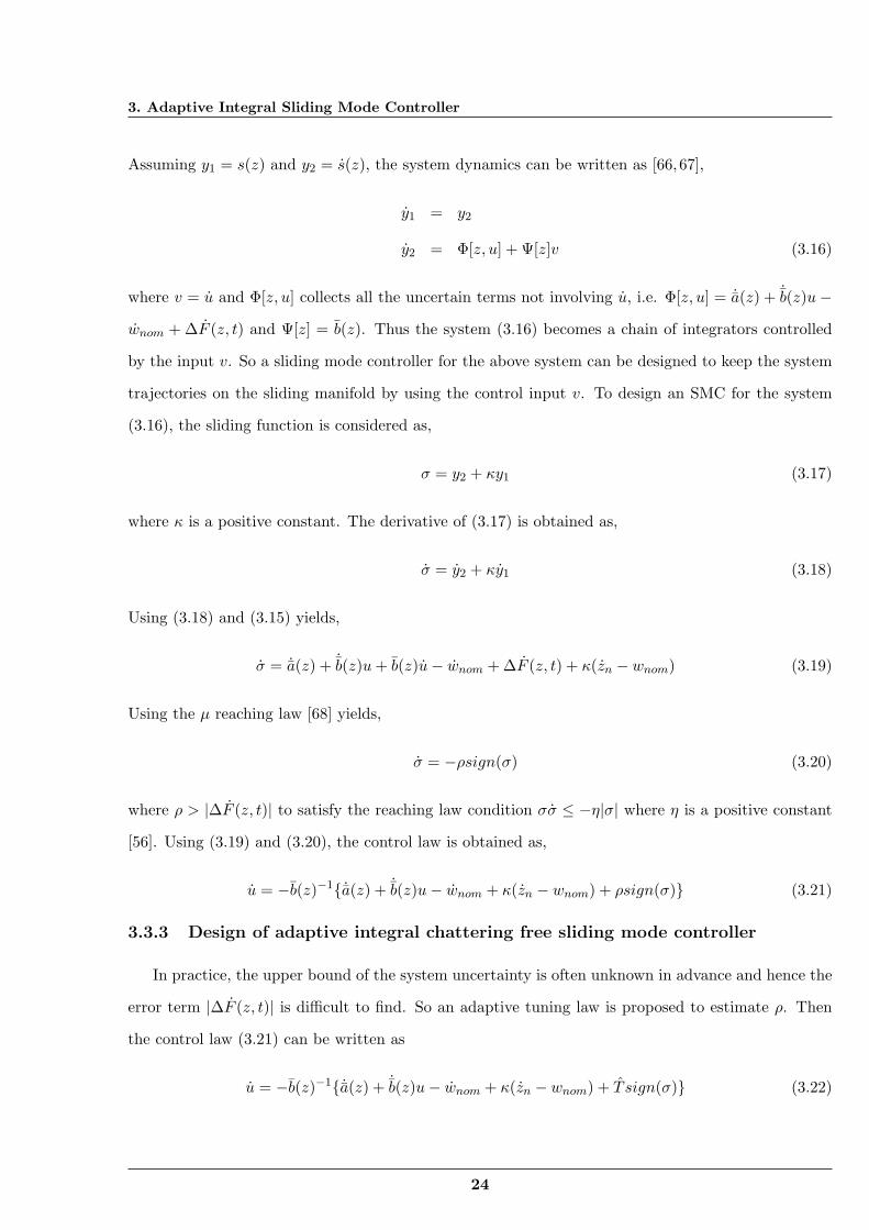
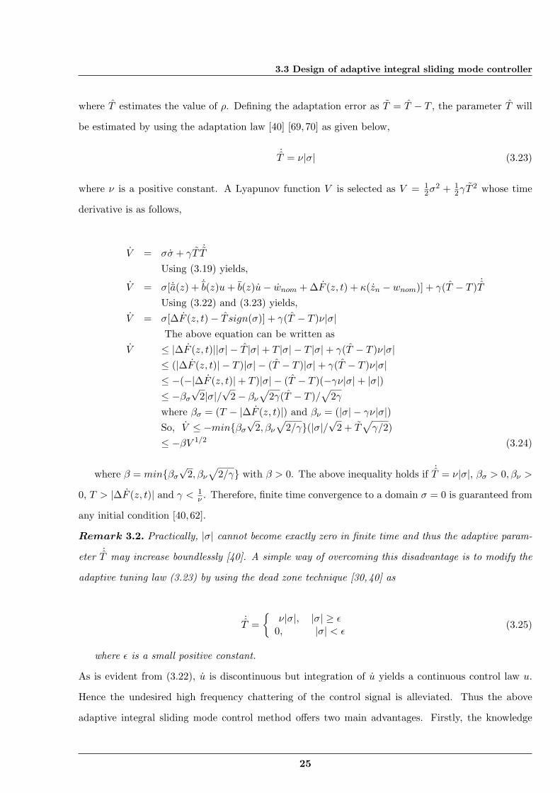
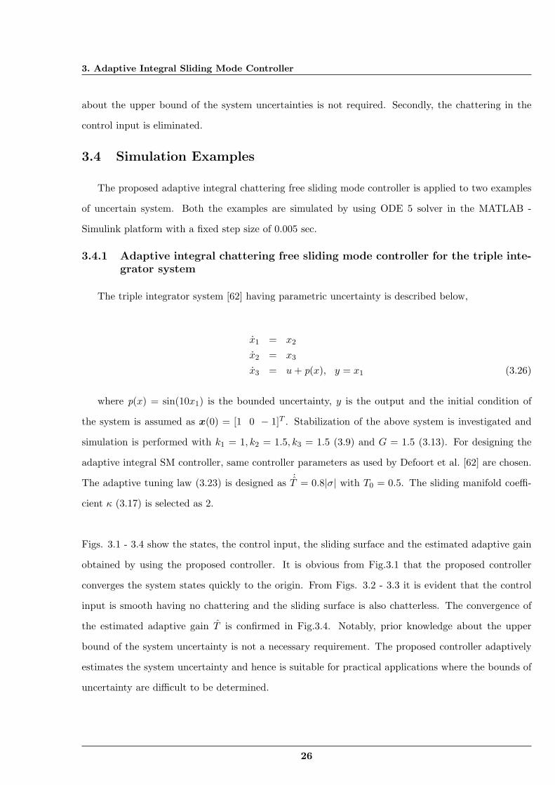
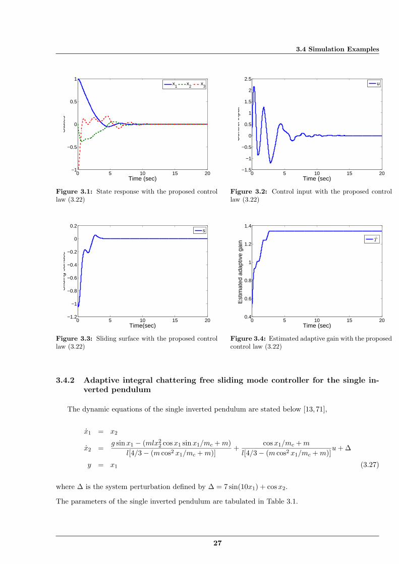
Figs. 3.1 - 3.4 show the states, the control input, the sliding surface and the estimated adaptive gain
obtained by using the proposed controller. It is obvious from Fig.3.1 that the proposed controller
converges the system states quickly to the origin. From Figs. 3.2 - 3.3 it is evident that the control
input is smooth having no chattering and the sliding surface is also chatterless. The convergence of
the estimated adaptive gain T is confirmed in Fig.3.4. Notably, prior knowledge about the upper
bound of the system uncertainty is not a necessary requirement. The proposed controller adaptively
estimates the system uncertainty and hence is suitable for practical applications where the bounds of
uncertainty are difficult to be determined.
26
3.4 Simulation Examples
0 5 10 15 20−1
−0.5
0
0.5
1
Time (sec)
Sta
tes
x1
x2
x3
Figure 3.1: State response with the proposed controllaw (3.22)
0 5 10 15 20−1.5
−1
−0.5
0
0.5
1
1.5
2
2.5
Time (sec)
Con
trol
inpu
t
u
Figure 3.2: Control input with the proposed controllaw (3.22)
0 5 10 15 20−1.2
−1
−0.8
−0.6
−0.4
−0.2
0
0.2
Time(sec)
Slid
ing
surf
ace
s
Figure 3.3: Sliding surface with the proposed controllaw (3.22)
0 5 10 15 200.4
0.6
0.8
1
1.2
1.4
Time (sec)
Est
imat
ed a
dapt
ive
gain
T
Figure 3.4: Estimated adaptive gain with the proposedcontrol law (3.22)
3.4.2 Adaptive integral chattering free sliding mode controller for the single in-verted pendulum
The dynamic equations of the single inverted pendulum are stated below [13,71],
x1 = x2
x2 =g sinx1 − (mlx2
2 cosx1 sinx1/mc +m)l[4/3 − (m cos2 x1/mc +m)]
+cosx1/mc +m
l[4/3 − (m cos2 x1/mc +m)]u+ ∆
y = x1 (3.27)
where ∆ is the system perturbation defined by ∆ = 7 sin(10x1) + cosx2.
The parameters of the single inverted pendulum are tabulated in Table 3.1.
27
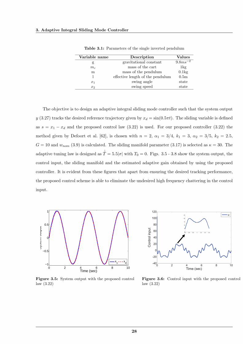
3. Adaptive Integral Sliding Mode Controller
Table 3.1: Parameters of the single inverted pendulum
Variable name Description Valuesg gravitational constant 9.8ms−2
mc mass of the cart 1kgm mass of the pendulum 0.1kgl effective length of the pendulum 0.5mx1 swing angle statex2 swing speed state
The objective is to design an adaptive integral sliding mode controller such that the system output
y (3.27) tracks the desired reference trajectory given by xd = sin(0.5πt). The sliding variable is defined
as s = x1 − xd and the proposed control law (3.22) is used. For our proposed controller (3.22) the
method given by Defoort et al. [62], is chosen with n = 2, α1 = 3/4, k1 = 3, α2 = 3/5, k2 = 2.5,
G = 10 and wnom (3.9) is calculated. The sliding manifold parameter (3.17) is selected as κ = 30. The
adaptive tuning law is designed as ˙T = 5.5|σ| with T0 = 0. Figs. 3.5 - 3.8 show the system output, the
control input, the sliding manifold and the estimated adaptive gain obtained by using the proposed
controller. It is evident from these figures that apart from ensuring the desired tracking performance,
the proposed control scheme is able to eliminate the undesired high frequency chattering in the control
input.
0 2 4 6 8 10−1
−0.5
0
0.5
1
Time (sec)
Sys
tem
out
put
x1
xd
Figure 3.5: System output with the proposed controllaw (3.22)
0 2 4 6 8 10-40
-20
0
20
40
60
80
100
120
Time (sec)
Co
ntr
ol in
pu
t
u
2.4 2.6 2.8 3 3.2 3.4 3.60
5
10
15
20
25
Figure 3.6: Control input with the proposed controllaw (3.22)
28
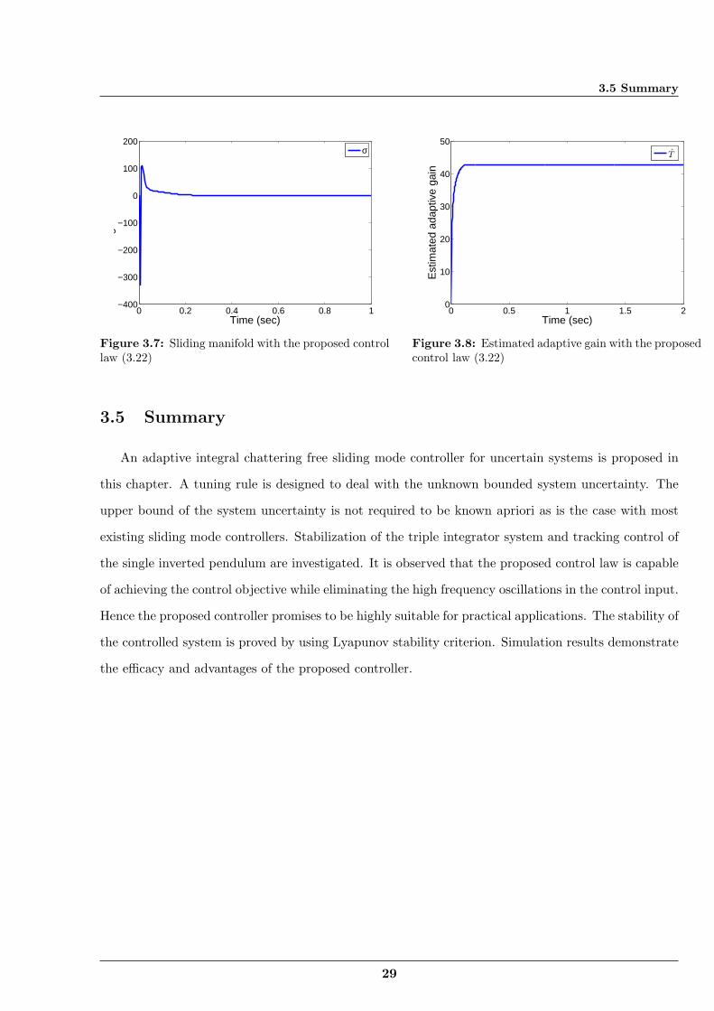
3.5 Summary
0 0.2 0.4 0.6 0.8 1−400
−300
−200
−100
0
100
200
Time (sec)
Slid
ing
man
ifold
σ
Figure 3.7: Sliding manifold with the proposed controllaw (3.22)
0 0.5 1 1.5 20
10
20
30
40
50
Time (sec)
Est
imat
ed a
dapt
ive
gain
T
Figure 3.8: Estimated adaptive gain with the proposedcontrol law (3.22)
3.5 Summary
An adaptive integral chattering free sliding mode controller for uncertain systems is proposed in
this chapter. A tuning rule is designed to deal with the unknown bounded system uncertainty. The
upper bound of the system uncertainty is not required to be known apriori as is the case with most
existing sliding mode controllers. Stabilization of the triple integrator system and tracking control of
the single inverted pendulum are investigated. It is observed that the proposed control law is capable
of achieving the control objective while eliminating the high frequency oscillations in the control input.
Hence the proposed controller promises to be highly suitable for practical applications. The stability of
the controlled system is proved by using Lyapunov stability criterion. Simulation results demonstrate
the efficacy and advantages of the proposed controller.
29
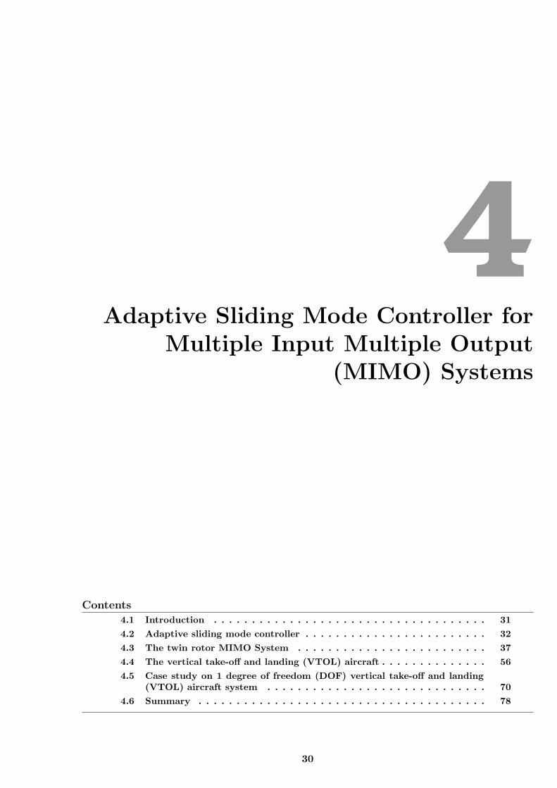
4Adaptive Sliding Mode Controller for
Multiple Input Multiple Output(MIMO) Systems
Contents
4.1 Introduction . . . . . . . . . . . . . . . . . . . . . . . . . . . . . . . . . . . . 31
4.2 Adaptive sliding mode controller . . . . . . . . . . . . . . . . . . . . . . . . 32
4.3 The twin rotor MIMO System . . . . . . . . . . . . . . . . . . . . . . . . . 37
4.4 The vertical take-off and landing (VTOL) aircraft . . . . . . . . . . . . . . 56
4.5 Case study on 1 degree of freedom (DOF) vertical take-off and landing(VTOL) aircraft system . . . . . . . . . . . . . . . . . . . . . . . . . . . . . 70
4.6 Summary . . . . . . . . . . . . . . . . . . . . . . . . . . . . . . . . . . . . . . 78
30
4.1 Introduction
4.1 Introduction
It is evident from the discussion so far that the sliding mode control (SMC) is a robust control
strategy which is insensitive to matched uncertainty affecting a dynamic system [43]. However, in
presence of mismatched perturbations, the property of asymptotical stability is, in general, hard to
achieve by using the traditional SMC technique [59]. One significant research finding is that the
stability of the system is guaranteed if the system trajectory is driven to a bounded region [31,72,73].
Hence when the system contains mismatched perturbations, the information about the upper bound
of perturbations is needed in order to achieve asymptotical stability [32, 74, 75]. A technique was
developed in [38] where asymptotic stability could be achieved without requiring the information about
the upper bound of the system uncertainties. Here adaptive mechanism was embedded in the controller
as well as in the sliding surface, but the control input obtained by using the above-mentioned method
was not smooth and high frequency chattering was present which made the algorithm substantially
difficult to apply practically.
In this chapter, a chattering free sliding mode control scheme for multiple input multiple output
(MIMO) systems with both matched and mismatched uncertainties is proposed. A tuning rule based
sliding mode is used to design the proposed controller in order to mitigate chattering and adaptive
tuning mechanism is employed for estimating the upper bound of the system uncertainty. The twin
rotor multi input multi output system (TRMS), which is a typical example of a coupled MIMO system
with mismatched uncertainty, is considered for design and validation purpose. The TRMS is divided
into a horizontal and a vertical subsystem and an adaptive sliding mode controller is designed for each
of the subsystems. Next the adaptive sliding mode controller is applied for stabilization of the vertical
take-off and landing (VTOL) aircraft system which is affected by both matched and mismatched
types of uncertainty. To show the effectiveness of the proposed control law, experimental studies are
conducted on a single degree of freedom (DOF) vertical take-off and landing (VTOL) aircraft system
to study the real time performance of the proposed adaptive sliding mode (SM) controller. The design
prerequisite of the sliding mode controller is complete knowledge about the state vector which is not
available in this example. Hence unavailable states of the 1 DOF VTOL are estimated by using an
extended state observer (ESO).
The outline of this chapter is as follows. Section 4.2 discusses the design procedure of the adaptive
sliding mode controller. The design strategy is demonstrated by taking the TRMS into consideration
31
4. Adaptive Sliding Mode Controller for Multiple Input Multiple Output (MIMO) Systems
in Section 4.3. In Section 4.4, effectiveness of this adaptive sliding mode controller is validated by
applying it for stabilization of the VTOL system. Experimental results obtained by applying the
adaptive sliding mode controller on the laboratory set-up QNET which is the prototype of VTOL
aircraft system are presented in Section 4.5. A brief summary of the chapter is presented in Section
4.6.
4.2 Adaptive sliding mode controller
Let us consider the following uncertain system
x = Ax+Bu+ f(x, t) (4.1)
where x ∈ Rn is the state vector, u ∈ Rm is the control input and the continuous function f(x, t)
represents matched and mismatched uncertainties together. Let us assume that the above system is
in the regular form requiring no transformation. Thus the system can be written as,
x1 = a11x1 + a12x2 + fu(x, t)
x2 = a21x1 + a22x2 +B2u+B2fm(x, t) (4.2)
where x1 ∈ Rn−m, x2 ∈ Rm, fu(x, t) is the mismatched perturbation and fm(x, t) is the matched one.
Let us consider the sliding surface given by
s = cx
= c1x1 + c2x2 (4.3)
where c1, c2 are matrices with proper dimension.
4.2.1 Stability during the sliding mode
During the sliding mode s = 0 and therefore (4.3) can be written as,
s = cx = c1x1 + c2x2 = 0
or, x2 = −c−12 c1x1 (4.4)
32
4.2 Adaptive sliding mode controller
where c2 is invertible.
Using (4.4) in the state space model (4.2) yields,
x1 = a11x1 − a12c−12 c1x1 + fu
= (a11 − a12c−12 c1)x1 + fu
= asx1 + fu (4.5)
where as = (a11−a12c−12 c1). Furthermore, fu is the uncertainty satisfying the condition ||fu|| ≤ λ||x1||
[8] where λ is a bounded positive constant.
Remark 4.1. The above assumption is a limitation on the uncertainties that can be tolerated by the
system. From the work in [74] [76] [77], these assumptions are fundamental and reasonable. The
structural requirement on the interconnection bounds is not essential because it can be easily extended
to a more general case (for example, [78] can be referred to).
It is to be noted that c1 and c2 are designed in such a way that the eigenvalues of as lie in the left
half of the s-plane and there exits a positive definite matrix P [74] such that
aTs P + Pas = −R (4.6)
where R is also a positive definite matrix. Let a Lyapunov function for the system be defined as
V2 = xT1 Px1. The time derivative of V2 is obtained as,
V2 = xT1 Px1 + xT1 Px1
= xT1 aTs Px1 + fTu Px1 + xT1 Pasx1 + xT1 Pfu
= xT1 (aTs P + Pas)x1 + fTu Px1 + xT1 Pfu
= −xT1Rx1 + 2xT1 Pfu (4.7)
It is known that [74] [75],
xT1Rx1 ≥ λmin(R)xT1 x1 = λmin(R)||x1||2 (4.8)
where λmin is the minimum eigen value and so,
V2 ≤ −λmin(R)||x1||2 + 2xT1 Pfu (4.9)
33
4. Adaptive Sliding Mode Controller for Multiple Input Multiple Output (MIMO) Systems
If there exists a bounded positive constant λ such that λ < 0.5λmin(R)/||P ||, then
2xT1 Pfu ≤ 2λ||P ||||x1||2 < λmin(R)||x1||2 (4.10)
and
V2 ≤ −λmin(R)||x1||2 + 2xT1 Pfu < 0 (4.11)
Hence the stability in the sliding mode is proved.
4.2.2 Design of the control law
The time derivative of sliding surface
s =d
dt(cx)
= cx(t)
= c(Ax+Bu+ f(x, t)) (4.12)
s = cAx+ cBu+ cf(x, t)
= cA2x+ cABu+ cBu+ (cAf(x, t) + cf(x, t)) (4.13)
Assuming s = y1(x) and s = y2(x), the system dynamics can be written as,
y1(x) = y2(x)
y2(x) = Φ[x, u] + Ψ[x]v (4.14)
where v = u and Φ[x, u] collects all the uncertain terms not involving u. So a sliding mode controller
for the above system can be designed to keep the system trajectories on the sliding manifold using the
control input u = v. Let the sliding function be considered as,
σ = y2(x) + κy1(x) (4.15)
where κ is a positive constant. Differentiating (4.15) yields,
σ = y2(x) + κy1(x) (4.16)
34
4.2 Adaptive sliding mode controller
Using (4.12), (4.13) and (4.16) yields,
σ = cA2x+ cABu+ cBu+ (cAf(x, t) + cf(x, t))
+κc(Ax+Bu+ f(x, t))
= cA2x+ κcAx+ (cAB + κcB)u+ cBu
+c(Af(x, t) + f(x, t) + κf(x, t)) (4.17)
Using the constant plus proportional reaching law gives rise to,
σ = −k1σ − k2sign(σ) (4.18)
Using (4.17) and (4.18), the control law is obtained as,
u = −(cB)−1((cA2 + κcA)x+ (cAB + κcB)u
+k1σ + k2sign(σ)) (4.19)
where k1 ≥ 0 and k2 > c(Af(x, t)+ f(x, t)+κf(x, t)) = c∇F = Q to satisfy the reaching law condition
σσ ≤ −η||σ||, where η is a positive constant.
Proof : A Lyapunov function is defined as V = 12σ
2 and using the control law it is easy to find that,
V = σσ
= σ[c∇F − k1σ − k2sign(σ)]
= σ[Q− k1σ − k2sign(σ)]
≤ Q||σ|| − k2||σ|| ≤ −η||σ|| (4.20)
Clearly, (4.20) implies that if k1 ≥ 0 and k2 > Q, control law (4.19) forces the sliding manifold σ to
zero in finite time.
4.2.3 Design of the adaptive tuning law
In practice, the uncertain term ∇F is often difficult to know. Hence an adaptive tuning law is
designed to determine k2. So (4.18) can be written as
σ = −k1σ − T sign(σ) (4.21)
35
4. Adaptive Sliding Mode Controller for Multiple Input Multiple Output (MIMO) Systems
where T estimates the value of k2.
Using (4.19) and (4.21), the control law is obtained as,
u = −(cB)−1((cA2 + κcA)x+ (cAB + κcB)u
+k1σ + T sign(σ)) (4.22)
Defining the adaptation error as T = T − T , the parameter T is estimated by using the adaptation
law [39,69,79]
˙T =
1γ||σ|| (4.23)
where γ is a positive constant. A Lyapunov function is defined as V = 12σ
2 + 12γT
2 and it is easy to
find that,
V = σσ + γT ˙T
= σ[c∇F − k1σ − T sign(σ)] + γ(T − T ) ˙T
= σ[Q− k1σ − T sign(σ)] + γ(T − T ) ˙T
≤ Q||σ|| − T ||σ|| ≤ −η||σ|| (4.24)
The above inequality holds if ˙T = 1
γ ||σ||, η > 0 and T > Q. This ensures the convergence of σ and
guarantees that the states converges to equilibrium asymptotically.
Remark 4.2. Practically, ||σ|| cannot become exactly zero in finite time and thus the adaptive pa-
rameter ˙T may increase boundlessly. A simple way of overcoming this disadvantage is to modify the
adaptive tuning law (4.23) by using the dead zone technique [30] as
˙T =
1γ ||σ||, ||σ|| ≥ ϵ
0, ||σ|| < ϵ(4.25)
where ϵ is a small positive constant.
As is evident from (4.19), u is free from any discontinuous part and so integration of u yields a
continuous control law u. Hence the undesired high frequency chattering of the control signal is
eliminated.
Thus the above adaptive SM control method offers two main advantages. Firstly, the knowledge about
36
4.3 The twin rotor MIMO System
the upper bound of the system uncertainties is not required. Secondly, the chattering in the control
input is removed.
4.3 The twin rotor MIMO System
In this section the problem of controlling the twin rotor MIMO system (TRMS), which is the
prototype of a helicopter, is addressed. The above-mentioned control law is used for the TRMS
affected by mismatched uncertainty.
The TRMS has been the object of research for control theorists for many years. The TRMS resembles
a nonlinear system with heavy cross coupling effects. Hence controlling the TRMS is quite challenging
and has gained a lot of research interest [8, 80–83]. An evolutionary computation based proportional
integral derivative (PID) controller has been proposed for addressing the tracking control problem in
the TRMS [84]. A fuzzy logic based linear quadratic regulator (LQR) control has been developed
to stabilize the TRMS in presence of high cross coupling [1]. In [1] the phase portrait technique has
been used for rule reduction and obtaining the model. In [85] a robust dead beat controller has been
designed for controlling the TRMS. Here the system was decoupled into two single input single output
(SISO) models and the cross coupling was considered as disturbance for each other.
In this section, a sliding mode (SM) controller is proposed for position control of the TRMS. In
the proposed design methodology, the mathematical model of the TRMS is pseudo decoupled into a
horizontal and a vertical subsystem. The cross coupling effect between the main rotor and the tail
rotor is considered as the uncertainty in the pseudo decoupled TRMS. An adaptive tuning law is
adopted to deal with the system uncertainty. The main benefit offered by this adaptive sliding mode
controller is that apriori knowledge about the upper bound of the system uncertainty is not needed.
A proportional integral (PI) sliding surface is designed for the vertical subsystem to remove the offset
in the pitch angle. Simulation results illustrate that our proposed adaptive sliding mode controller
shows better tracking performance with lesser control effort as compared to PID controllers [84]. Even
the presence of an external disturbance in the horizontal as well as the vertical subsystem does not
degrade the performance of the proposed adaptive sliding mode controller.
4.3.1 TRMS Description
The TRMS is a laboratory setup resembling a flight control system as shown in Fig. 4.1. The
TRMS is a highly coupled nonlinear multi input multi output (MIMO) system. The TRMS consists
37
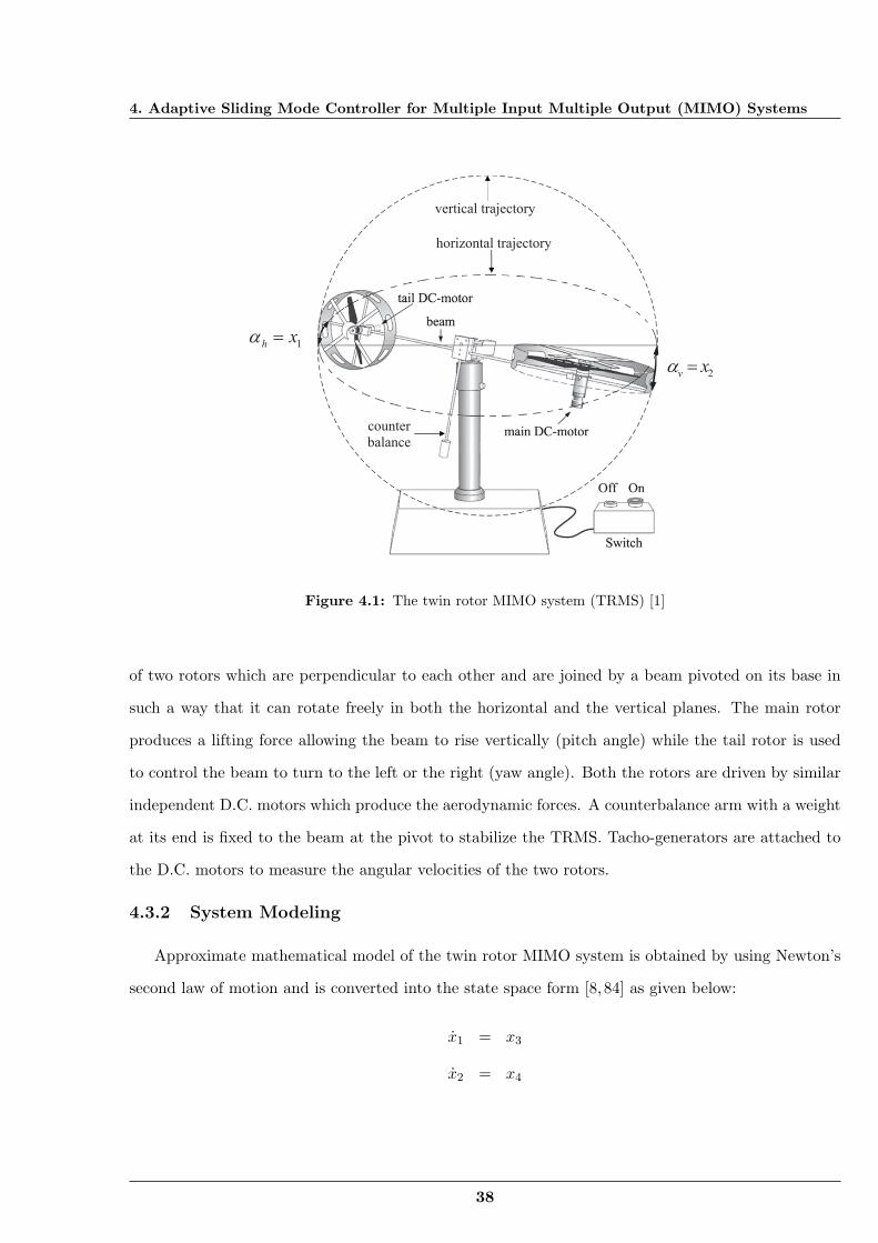
4. Adaptive Sliding Mode Controller for Multiple Input Multiple Output (MIMO) Systems
horizontal trajectory
vertical trajectory
1hx !
2vx !
counter
balance
Figure 4.1: The twin rotor MIMO system (TRMS) [1]
of two rotors which are perpendicular to each other and are joined by a beam pivoted on its base in
such a way that it can rotate freely in both the horizontal and the vertical planes. The main rotor
produces a lifting force allowing the beam to rise vertically (pitch angle) while the tail rotor is used
to control the beam to turn to the left or the right (yaw angle). Both the rotors are driven by similar
independent D.C. motors which produce the aerodynamic forces. A counterbalance arm with a weight
at its end is fixed to the beam at the pivot to stabilize the TRMS. Tacho-generators are attached to
the D.C. motors to measure the angular velocities of the two rotors.
4.3.2 System Modeling
Approximate mathematical model of the twin rotor MIMO system is obtained by using Newton’s
second law of motion and is converted into the state space form [8,84] as given below:
x1 = x3
x2 = x4
38
4.3 The twin rotor MIMO System
x3 =1jh
[ltSfFh(wt)cosx2 − khx3 − x3x4(D −E)sin2x2 − jmrwm(x6)x4sinx2
+jmrTmr
(uv − x6)dwm(x6)dx6
cosx2]
x4 = 9.1[lmSfFv(wm) − g(0.0099cosx2 + 0.0168sinx2) − kvx4]
+9.1[−0.0252x23sin2x2 +
jtrTtr
(uh − x5)dwt(x5)dx5
]
x5 =1Ttr
(uh − x5)
x6 =1Tmr
(uv − x6) (4.26)
With uv(uh) being the input voltage of the DC motor for the main (tail) propeller, the armature
current iv(ih) can be obtained by solving the following differential equations
divdt
=1Tmr
(uv − iv)
dihdt
=1Ttr
(uh − ih) (4.27)
where x1 = αh is the yaw angle, x2 = αv is the pitch angle, x3 = Ωh is the angular velocity around
the horizontal axis, x4 = Ωv is the angular velocity around the vertical axis, x5 = ih is the armature
current of the tail propeller subsystem, x6 = iv is the armature current of the main propeller subsystem.
Furthermore, lm(lt) is the main (tail) length of the beam, jmr(jtr) is the moment of inertia for the main
(tail) propeller subsystem, Tmr(Ttr) is the time constant of the main (tail) motor-propeller system and
ωm(ωt) is the rotational speed of the main (tail) rotor DC motor. Moreover, kv(kh) is the friction
constant of the main (tail) propeller subsystem, Sf is the balanced scale and uv(uh) is the control
input for the main (tail) DC motor. The propulsive force to move the joined beam in the vertical
(horizontal) direction is denoted by Fv(Fh) which is approximately described by a nonlinear function of
the angular velocity ωm(ωt). Gravitational acceleration is symbolized as g and D, E, G are constants.
Furthermore,
jh = Dsin2x2 + Ecos2x2 +G
ωm(x6) = 90.99x66 + 599.73x5
6 − 129.26x46 − 1283.64x3
6 + 63.45x26 + 1283.41x6
ωt(x5) = 2020x55 − 194.69x4
5 − 4283.15x35 + 262.27x2
5 + 3768.83x5
39
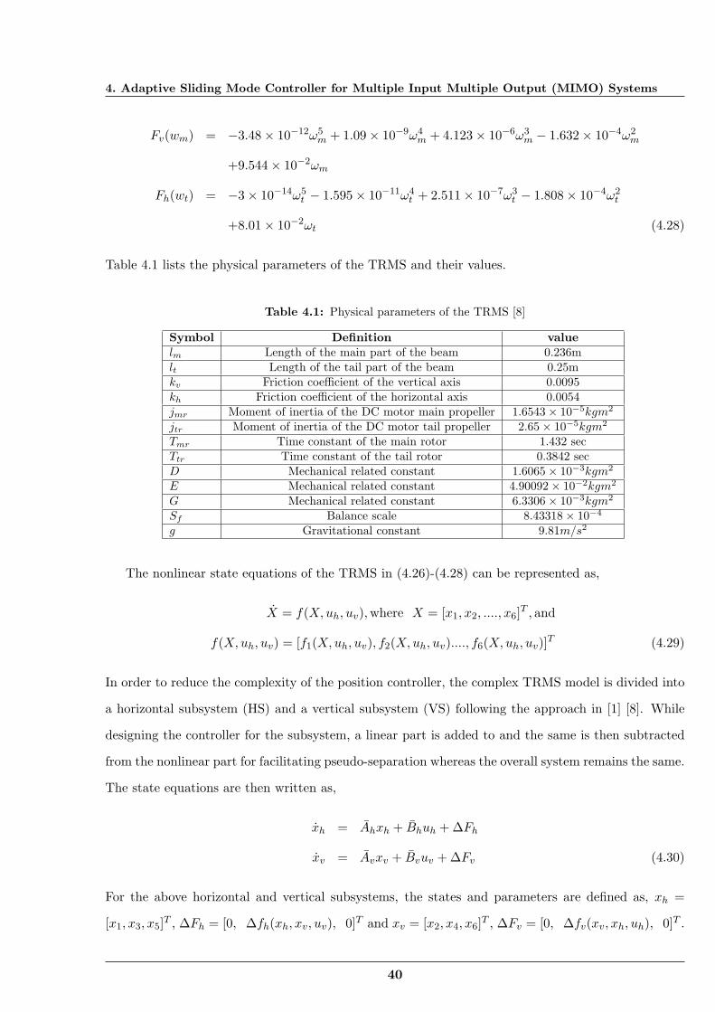
4. Adaptive Sliding Mode Controller for Multiple Input Multiple Output (MIMO) Systems
Fv(wm) = −3.48 × 10⁻¹²ω5m + 1.09 × 10⁻⁹ω4
m + 4.123 × 10⁻⁶ω3m − 1.632 × 10⁻⁴ω2
m
+9.544 × 10⁻²ωm
Fh(wt) = −3 × 10⁻¹⁴ω5t − 1.595 × 10⁻¹¹ω4
t + 2.511 × 10⁻⁷ω3t − 1.808 × 10⁻⁴ω2
t
+8.01 × 10⁻²ωt (4.28)
Table 4.1 lists the physical parameters of the TRMS and their values.
Table 4.1: Physical parameters of the TRMS [8]
Symbol Definition valuelm Length of the main part of the beam 0.236mlt Length of the tail part of the beam 0.25mkv Friction coefficient of the vertical axis 0.0095kh Friction coefficient of the horizontal axis 0.0054jmr Moment of inertia of the DC motor main propeller 1.6543 × 10⁻⁵kgm2
jtr Moment of inertia of the DC motor tail propeller 2.65 × 10⁻⁵kgm2
Tmr Time constant of the main rotor 1.432 secTtr Time constant of the tail rotor 0.3842 secD Mechanical related constant 1.6065 × 10⁻³kgm2
E Mechanical related constant 4.90092 × 10⁻²kgm2
G Mechanical related constant 6.3306 × 10⁻³kgm2
Sf Balance scale 8.43318 × 10⁻⁴
g Gravitational constant 9.81m/s2
The nonlinear state equations of the TRMS in (4.26)-(4.28) can be represented as,
X = f(X,uh, uv),where X = [x1, x2, ...., x6]T , and
f(X,uh, uv) = [f1(X,uh, uv), f2(X,uh, uv)...., f6(X,uh, uv)]T (4.29)
In order to reduce the complexity of the position controller, the complex TRMS model is divided into
a horizontal subsystem (HS) and a vertical subsystem (VS) following the approach in [1] [8]. While
designing the controller for the subsystem, a linear part is added to and the same is then subtracted
from the nonlinear part for facilitating pseudo-separation whereas the overall system remains the same.
The state equations are then written as,
xh = Ahxh + Bhuh + ∆Fh
xv = Avxv + Bvuv + ∆Fv (4.30)
For the above horizontal and vertical subsystems, the states and parameters are defined as, xh =
[x1, x3, x5]T , ∆Fh = [0, ∆fh(xh, xv, uv), 0]T and xv = [x2, x4, x6]T , ∆Fv = [0, ∆fv(xv, xh, uh), 0]T .
40
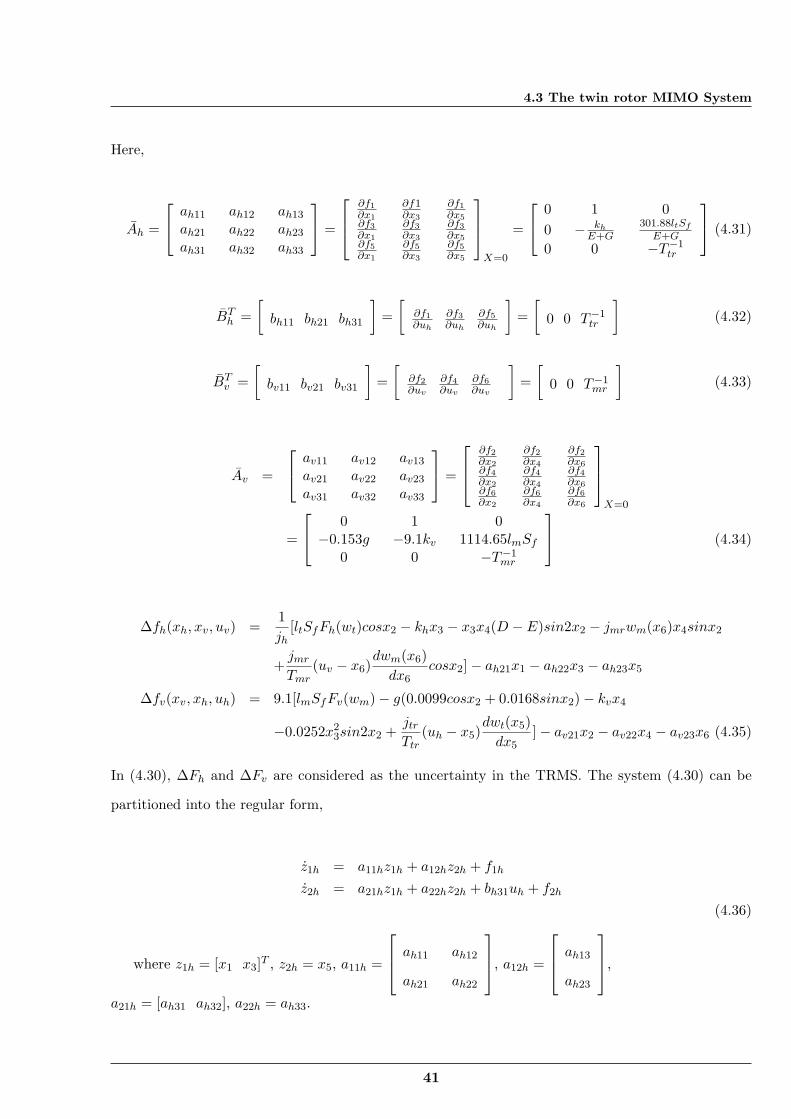
4.3 The twin rotor MIMO System
Here,
Ah =
ah11 ah12 ah13
ah21 ah22 ah23
ah31 ah32 ah33
=
∂f1∂x1
∂f1∂x3
∂f1∂x5
∂f3∂x1
∂f3∂x3
∂f3∂x5
∂f5∂x1
∂f5∂x3
∂f5∂x5
X=0
=
0 1 00 − kh
E+G301.88ltSf
E+G
0 0 −T−1tr
(4.31)
BTh =
[bh11 bh21 bh31
]=[
∂f1∂uh
∂f3∂uh
∂f5∂uh
]=[
0 0 T−1tr
](4.32)
BTv =
[bv11 bv21 bv31
]=[
∂f2∂uv
∂f4∂uv
∂f6∂uv
]=[
0 0 T−1mr
](4.33)
Av =
av11 av12 av13
av21 av22 av23
av31 av32 av33
=
∂f2∂x2
∂f2∂x4
∂f2∂x6
∂f4∂x2
∂f4∂x4
∂f4∂x6
∂f6∂x2
∂f6∂x4
∂f6∂x6
X=0
=
0 1 0−0.153g −9.1kv 1114.65lmSf
0 0 −T−1mr
(4.34)
∆fh(xh, xv, uv) =1jh
[ltSfFh(wt)cosx2 − khx3 − x3x4(D − E)sin2x2 − jmrwm(x6)x4sinx2
+jmrTmr
(uv − x6)dwm(x6)dx6
cosx2] − ah21x1 − ah22x3 − ah23x5
∆fv(xv, xh, uh) = 9.1[lmSfFv(wm) − g(0.0099cosx2 + 0.0168sinx2) − kvx4
−0.0252x23sin2x2 +
jtrTtr
(uh − x5)dwt(x5)dx5
] − av21x2 − av22x4 − av23x6 (4.35)
In (4.30), ∆Fh and ∆Fv are considered as the uncertainty in the TRMS. The system (4.30) can be
partitioned into the regular form,
z1h = a11hz1h + a12hz2h + f1h
z2h = a21hz1h + a22hz2h + bh31uh + f2h
(4.36)
where z1h = [x1 x3]T , z2h = x5, a11h =
ah11 ah12
ah21 ah22
, a12h =
ah13
ah23
,
a21h = [ah31 ah32], a22h = ah33.
41
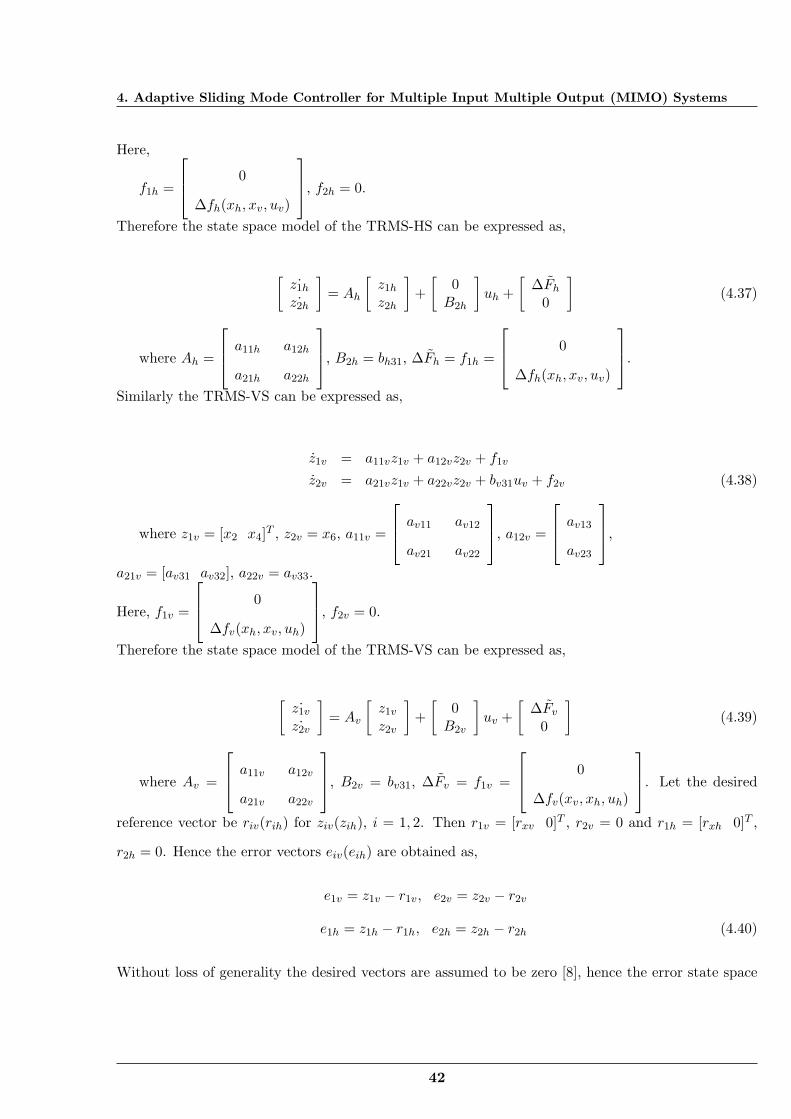
4. Adaptive Sliding Mode Controller for Multiple Input Multiple Output (MIMO) Systems
Here,
f1h =
0
∆fh(xh, xv, uv)
, f2h = 0.
Therefore the state space model of the TRMS-HS can be expressed as,
[˙z1h˙z2h
]= Ah
[z1hz2h
]+[
0B2h
]uh +
[∆Fh
0
](4.37)
where Ah =
a11h a12h
a21h a22h
, B2h = bh31, ∆Fh = f1h =
0
∆fh(xh, xv, uv)
.
Similarly the TRMS-VS can be expressed as,
z1v = a11vz1v + a12vz2v + f1v
z2v = a21vz1v + a22vz2v + bv31uv + f2v (4.38)
where z1v = [x2 x4]T , z2v = x6, a11v =
av11 av12
av21 av22
, a12v =
av13
av23
,
a21v = [av31 av32], a22v = av33.
Here, f1v =
0
∆fv(xh, xv, uh)
, f2v = 0.
Therefore the state space model of the TRMS-VS can be expressed as,
[˙z1v˙z2v
]= Av
[z1vz2v
]+[
0B2v
]uv +
[∆Fv
0
](4.39)
where Av =
a11v a12v
a21v a22v
, B2v = bv31, ∆Fv = f1v =
0
∆fv(xv, xh, uh)
. Let the desired
reference vector be riv(rih) for ziv(zih), i = 1, 2. Then r1v = [rxv 0]T , r2v = 0 and r1h = [rxh 0]T ,
r2h = 0. Hence the error vectors eiv(eih) are obtained as,
e1v = z1v − r1v, e2v = z2v − r2v
e1h = z1h − r1h, e2h = z2h − r2h (4.40)
Without loss of generality the desired vectors are assumed to be zero [8], hence the error state space
42
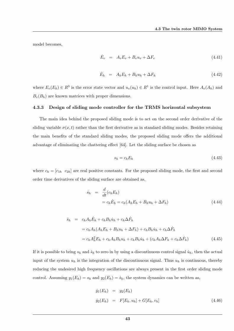
4.3 The twin rotor MIMO System
model becomes,
Ev = AvEv +Bvuv + ∆Fv (4.41)
Eh = AhEh +Bhuh + ∆Fh (4.42)
where Ev(Eh) ∈ R3 is the error state vector and uv(uh) ∈ R1 is the control input. Here Av(Ah) and
Bv(Bh) are known matrices with proper dimensions.
4.3.3 Design of sliding mode controller for the TRMS horizontal subsystem
The main idea behind the proposed sliding mode is to act on the second order derivative of the
sliding variable σ(x, t) rather than the first derivative as in standard sliding modes. Besides retaining
the main benefits of the standard sliding modes, the proposed sliding mode offers the additional
advantage of eliminating the chattering effect [64]. Let the sliding surface be chosen as
sh = chEh (4.43)
where ch = [c1h c2h] are real positive constants. For the proposed sliding mode, the first and second
order time derivatives of the sliding surface are obtained as,
sh =d
dt(chEh)
= chEh = ch(AhEh +Bhuh + ∆Fh) (4.44)
sh = chAhEh + chBhuh + ch∆Fh
= chAh(AhEh +Bhuh + ∆Fh) + chBhuh + ch∆Fh
= chA2hEh + chAhBhuh + chBhuh + (chAh∆Fh + ch∆Fh) (4.45)
If it is possible to bring sh and sh to zero in by using a discontinuous control signal uh, then the actual
input of the system uh is the integration of the discontinuous signal. Thus uh is continuous, thereby
reducing the undesired high frequency oscillations are always present in the first order sliding mode
control. Assuming y1(Eh) = sh and y2(Eh) = sh, the system dynamics can be written as,
y1(Eh) = y2(Eh)
y2(Eh) = F [Eh, uh] +G[Eh, vh] (4.46)
43
4. Adaptive Sliding Mode Controller for Multiple Input Multiple Output (MIMO) Systems
where vh = uh and F [Eh, uh] collects all the uncertain terms not involving uh. Thus the horizontal
subsystem (4.30) becomes a chain of integrators controlled by the input uh. So a sliding mode controller
for the above system can be designed to keep the system trajectories in the sliding manifold using the
control input vh. To design a SMC for the system (4.42), the sliding function is considered as,
σh = y2(Eh) + κhy1(Eh) (4.47)
where κh is a positive constant. Taking the derivative of (4.47) we get,
σh = y2(Eh) + κhy1(Eh) (4.48)
From (4.44), (4.45) and (4.46) we have,
y1(Eh) = ch(AhEh +Bhuh + ∆Fh)
y2(Eh) = chA2hEh + chAhBhuh + chBhuh + chAh∆Fh + ch∆Fh (4.49)
Using (4.48) and (4.49) we have,
σh = chA2hEh + chAhBhuh + chBhuh + chAh∆Fh + ch∆Fh + κh(ch(AhEh +Bhuh + ∆Fh))
= chA2hEh + κhchAhEh + (chAhBh + κhchBh)uh + chBhuh
+(chAh∆Fh + ch∆Fh) + κhch∆Fh (4.50)
For designing the adaptive part of the control law, we consider
σh = −k1hσh − k2hsign(σh) (4.51)
Using (4.50) and (4.51), the control law is obtained as,
uh = −(chBh)−1((chA2h + κhchAh)Eh + (chAhBh + κhchBh)uh + k1hσh + k2hsign(σh)) (4.52)
where k1h ≥ 0 and k2h > ch(Ah∆Fh + ∆Fh + κh∆Fh) = ch∇Fh = Qh to satisfy the reaching law
σhσh ≤ −ηh|σh|, where ηh > 0 [56]. Let us assume that there exits a bounded positive constant λ′h
such that, ||∇Fh|| ≤ λ′h||Eh|| [8] and Qh = λ′hch||Eh|| ≥ 0.
44
4.3 The twin rotor MIMO System
4.3.4 Design of adaptive tuning law for the horizontal subsystem
In practice the bound of uncertainty is often not known and hence the error term ||Eh|| is difficult
to know. So an adaptive tuning law is designed to determine k2h. Then the time derivative of the
control law (4.52) can be written as
uh = −(chBh)−1[(chA2h + κhchAh)Eh + (chAhBh + κhchBh)uh + k1hσh + Thsign(σh)] (4.53)
and consequently the actual control law can be obtained as,
uh = −(chBh)−1
∫ t
0[(chA2
h + κhchAh)Eh + (chAhBh + κhchBh)uh + k1hσh + Thsign(σh)]dτ (4.54)
where chBh is nonsingular, sign(σh) is the sign function and Th is the unknown bound which will be
estimated adaptively.
Defining the adaptation error as Th = Th − Th, where Th is the actual gain, the parameter Th will be
estimated by using the adaptation law
˙Th =
1γh
|σh| (4.55)
and γh > 0 is designed positive constant, Th(0) is the initial condition. A Lyapunov function is selected
as V1h = 12σ
2h + 1
2γhT2h whose time derivative is as follows,
V1h = σhσh + γhTh˙Th
= σh[ch∇Fh − k1hσh − Thsign(σh)] + γh(Th − Th)˙Th
= σh[Qh − k1hσh − Thsign(σh)] + γh(Th − Th)˙Th
≤ Qh|σh| − Th|σh|
≤ −ηh|σh| (4.56)
The above inequality holds if ˙Th = 1
γh|σh|, ηh > 0 and Th > Qh. Considering (4.55) and (4.56), it is
straightforward to verify that V1h ≤ −ηh|σh|, where ηh > 0. This ensures the convergence of σh and
guarantees that the states converge to the equilibrium asymptotically.
The adaptive law (4.55) is modified by using dead zone technique [30] as
˙Th =
1γh|σh|, |σh| ≥ ϵh
0, |σh| < ϵh
(4.57)
45
4. Adaptive Sliding Mode Controller for Multiple Input Multiple Output (MIMO) Systems
where ϵh is a small positive constant.
Initially the adaptation gain parameter γh is so chosen that it is smaller than the upper bound of
the system uncertainties. However, this is not really a restriction of the method since one can freely
choose a sufficiently small number.
4.3.5 Stability during the sliding mode
During the sliding mode sh = 0 and therefore (4.43) can be written as,
sh = chEh = c1he1h + c2he2h = 0
or, e2h = −c−12h c1he1h (4.58)
where c2h is invertible.
Using (4.58) in the error state space model (4.42), we get
e1h = a11he1h − a12hc−12h c1he1h + ∆Fh
= (a11h − a12hc−12h c1h)e1h + ∆Fh = ahse1h + ∆Fh (4.59)
where ahs = (a11h − a12hc−12h c1h). Furthermore, ∆Fh is the uncertainty satisfying the condition
||∆Fh|| ≤ λh||e1h|| [8]. It is to be noted that c1h and c2h are designed in such a way that the
eigenvalues of (a11h − a12hc−12h c1h) lie in the left half of the s-plane and there exists a positive definite
matrix Ph [74] such that
aThsPh + Phahs = −Rh (4.60)
where Rh is also a positive definite matrix. Let a Lyapunov function for the system be defined as
V2h = eT1hPhe1h. The time derivative of V2h is obtained as,
V2h = eT1hPhe1h + eT1hPhe1h
= eT1haThsPhe1h + ∆F Th Phe1h + eT1hPhahse1h + eT1hPh∆Fh
= eT1h(aThsPh + Phahs)e1h + ∆FhPhe1h + eT1hPh∆Fh
= −eT1hRhe1h + 2eT1hPh∆Fh (4.61)
It is known that [74] [75],
eT1hRhe1h ≥ λmin(Rh)eT1he1h = λmin(Rh)||e1h||2 (4.62)
46
4.3 The twin rotor MIMO System
where λmin is the minimum eigen value and so,
V2h ≤ −λmin(Rh)||e1h||2 + 2eT1hPh∆Fh (4.63)
If there exists a bounded positive constant λh such that λh < 0.5λmin(Rh)/||Ph||, then
2eT1hPh∆Fh ≤ 2λh||Ph||||e1h||2 < λmin(Rh)||e1h||2 (4.64)
and
V2h ≤ −λmin(Rh)||e1h||2 + 2eT1hPh∆Fh < 0 (4.65)
Hence the stability in the sliding mode is proved.
4.3.6 Design of sliding mode controller for the TRMS vertical subsystem
As the gravity force affects the dynamics of the vertical subsystem of the TRMS, it is difficult to
control the pitch angle at a desired reference location. In order to reduce the offset of the pitch angle,
a proportional plus integral sliding surface is designed for the vertical subsystem. Let us consider the
error state space model of the vertical subsystem given by (4.41),
Ev = AvEv +Bvuv + ∆Fv
(4.66)
where Ev ∈ R3 is the error state vector and uv ∈ R1 is the control input. Here Av and Bv are known
matrices with proper dimensions. A proportional plus integral sliding surface is chosen as,
sv = cvEv + c3v
∫ t
0e1vdτ (4.67)
where cv = [c1v c2v] are real positive constants and c3v is also a real positive constant whose selection
criterion is to be discussed in Section 4.3.8. For the proposed sliding mode, the first and second order
time derivatives of sv need to be considered. Thus we have,
sv =d
dt(cvEv + c3v
∫ t
0e1vdτ)
= cvEv + c3ve1v
= cv(AvEv +Bvuv + ∆Fv) + c3ve1v (4.68)
47
4. Adaptive Sliding Mode Controller for Multiple Input Multiple Output (MIMO) Systems
sv = cvAvEv + cvBvuv + cv∆Fv + c3v e1v
= cvAv(AvEv +Bvuv + ∆Fv) + cvBvuv + cv∆Fv + c3v e1v
= cvA2vEv + cvAvBvuv + cvBvuv + c3v e1v + cv(Av∆Fv + ∆Fv) (4.69)
By following a similar procedure as described earlier in Section 4.3.3, the following is obtained in the
case of TRMS VS,
σv = (cvA2v + κvcvAv)Ev + (cvAvBv + κvcvBv)uv + cvBvuv + c3v e1v
+κvc3ve1v + cv(Av∆Fv + ∆Fv) + κvcv∆Fv (4.70)
where κv is a positive constant. For designing the adaptive part of the control law, we consider [68]
σv = −k1vσv − k2vsign(σv) (4.71)
Using (4.70) and (4.71), the control law is obtained as,
uv = −(cvBv)−1[(cvA2v + κvcvAv)Ev + (cvAvBv + κvcvBv)uv
+c3v e1v + κvc3ve1v + k1vσv + k2vsign(σv)] (4.72)
where k1v ≥ 0 and k2v > cv(Av∆Fv + ∆Fv) + κvcv∆Fv = cv∇Fv = Qv to satisfy the reaching
law σvσv ≤ −ηv|σv| [56]. Let us assume that there exits a bounded positive constant λ′v such that,
||∇Fv|| ≤ λ′v||Ev|| [8] and Qv = λ′vcv||Ev|| ≥ 0.
4.3.7 Design of adaptive tuning law for the vertical subsystem
An adaptive tuning law is designed to determine k2v and so (4.72) can be written as [75]
uv = −(cvBv)−1[(cvA2v + κvcvAv)Ev + (cvAvBv + κvcvBv)uv
+c3v e1v + κvc3ve1v + k1vσv + Tvsign(σv)] (4.73)
where Tv estimates the value of k2v. The actual control is obtained as,
uv = −(cvBv)−1
∫ t
0[(cvA2
v + κvcvAv)Ev + (cvAvBv + κvcvBv)uv
+c3v e1v + κvc3ve1v + k1vσv + Tvsign(σv)]dτ (4.74)
48
4.3 The twin rotor MIMO System
The parameter Tv is estimated as [69] [70]
˙Tv =
1γv
|σv| (4.75)
where γv is a positive constant. A Lyapunov function is chosen as V1v = 12σ
2v + 1
2γvT2v whose time
derivative is obtained as,
V1v = σvσv + γvTv˙Tv
= σv[cv∇Fv − k1vσv − Tvsign(σv)] + γv(Tv − Tv)˙Tv
= σv[Qv − k1vσv − Tvsign(σv)] + γv(Tv − Tv)˙Tv
≤ Qv|σv| − Tv|σv|
≤ −ηv|σv| (4.76)
The above inequality holds if ˙Tv = 1
γv|σv| and Tv > Qv.
The adaptive law (4.75) is modified using the dead zone technique [30] as
˙Tv =
1γv|σv|, |σv| ≥ ϵv
0, |σv| < ϵv
(4.77)
where ϵv is a small positive constant.
The above control law (4.74) is free from any discontinuous part and hence chattering is reduced.
4.3.8 Stability of the sliding surface
During the sliding mode sv = 0 and therefore (4.67) can be written as,
sv = c1ve1v + c2ve2v + c3v
∫ t
0e1vdτ = 0
or, e2v = −c−12v (c1ve1v + c3v
∫ t
0e1vdτ) (4.78)
Using (4.41), we have
e1v = a11ve1v − a12vc−12v (c1ve1v + c3v
∫ t
0e1v dτ) + ∆Fv
= (a11v − a12vc−12v c1v)e1v − a12vc
−12v c3v
∫ t
0e1v dτ + ∆Fv
= avse1v − avt
∫ t
0e1v dτ + ∆Fv (4.79)
49
4. Adaptive Sliding Mode Controller for Multiple Input Multiple Output (MIMO) Systems
where avs = (a11v − a12vc−12v c1v) =
avs11 avs12
avs21 avs22
and avt = a12vc−12v c1v =
avt11 avt12
avt21 avt22
Let e1v = [e11v e12v]T and ∫ t
0e12v dτ = e11v (4.80)
A new state variable χ1 is defined as χ1 =∫ t0 e11v dτ and hence χ1 = e11v. Thus (4.79) can be
represented as,
χ =
χ1
e11v
e12v
=
0 1 00 0 1
−avt21 avs21 − avt22 avs22
χ1
e11v
e12v
+[
0∆Fv
]
= avvχ+[
0∆Fv
]= avvχ+ ∆Fvv (4.81)
where ∆Fvv = [0 ∆Fv]T . It is clear that ||∆Fvv|| = ||∆Fv||. Here c1v, c2v and c3v are designed in
such a way that the eigenvalues of (a11v − a12vc−12v c1v) lie in the left half of the s-plane and there exits
a positive definite matrix Pv such that
aTvvPv + Pvavv = −Rv (4.82)
where Rv is also a positive definite matrix. In the TRMS -VS, ∆Fvv satisfies ||∆Fvv|| ≤ λv||χ|| with
λv < 0.5λmin(Rv)/||Pv||. So the TRMS-VS is stable in the sliding mode. Let a Lyapunov function for
the system be selected as V2v = χTPvχ whose time derivative is obtained as,
V2v = χTPvχ+ χTPvχ
= χTaTvvPvχ+ ∆F TvvPvχ+ χTPvavvχ+ χTPv∆Fvv
= χT (aTvvPvχ+ Pvavv)χ+ ∆F TvvPvχ+ χTPv∆Fvv
= −χTRvχ+ 2χTPv∆Fvv (4.83)
It is known that [8]
χTRvχ ≥ λmin(Rv)χTχ = λmin(Rv)||χ||2 (4.84)
and V2v ≤ −λmin(Rv)||χ||2 + 2χTPv∆Fvv if λv < 0.5λmin(Rv)/||Pv||, then
2χTPv∆Fvv ≤ 2λv||Pv||||χ||2 < λmin(Rv)||χ||2 (4.85)
50
4.3 The twin rotor MIMO System
Therefore, V2v ≤ −λmin(Rv)||χ||2+2χTPv∆Fvv < 0. Hence the stability in the sliding mode is proved.
Remark 4.3. In designing the control law for the horizontal and vertical subsystems, the terms sh
and sv are needed. However, these derivative terms can neither be directly obtained nor measured.
Direct differentiation on sh(sv) is highly undesirable as practical measurement of sh(sv) in real time
application will contain high frequency noise. The first/higher order Levant’s exact differentiator [25]
[64] can be used for the estimation of sh(sv). A first order real time differentiator has the form,
z0 = −λ1|z0 − sh(sv)|1/2sign(z0 − sh(sv)) + z1
z1 = −λ2sign(z0 − sh(sv)) (4.86)
where λ1 > 0 and λ2 > 0 are the design parameters and the estimators are designed as sh(sv) = z1.
4.3.9 Simulation results
The proposed adaptive sliding mode controller is applied to the TRMS [8] and the performance
of the controlled system is studied by carrying out simulations using MATLAB ODE 4 solver with a
fixed step size of 0.01sec. The parameters used for the TRMS are as listed in Table 4.1.
4.3.10 Control parameters for the horizontal subsystem
In the horizontal subsystem, the sliding surface parameters ch = [c1h c2h] are chosen as c1h = [11 7]
and c2h = [7] to satisfy the condition (4.60). The values of the reaching mode coefficient k1h and
adaptive tuning parameter γh are chosen as 1.0 and 10 respectively (4.51, 4.55) by using the condition
given in Section 4.3.4. The value of κh (4.47) is chosen as 2.0. The adaptive tuning law is formed as˙Th = 0.1|σh| and Th(0) = 0.7 (4.55). The positive definite matrices Ph and Rh satisfying the stability
condition are selected as
Ph =[
122.27 27.2827.28 53.24
], Rh =
[98.61 7.987.98 78.29
](4.87)
The above values of Ph and Rh are found suitable for the simulation example.
4.3.11 Control parameters for the vertical subsystem
For the vertical subsystem, the PI sliding surface parameters cv = [c1v c2v] (4.67) are chosen as
c1v = [11 8], c2v = 12 and c3v = [7 0.5] to satisfy the condition mentioned in Section 4.3.5. The values
of the reaching mode coefficient k1v and the adaptive tuning parameter γv are selected as 1.3 and 1.25
51
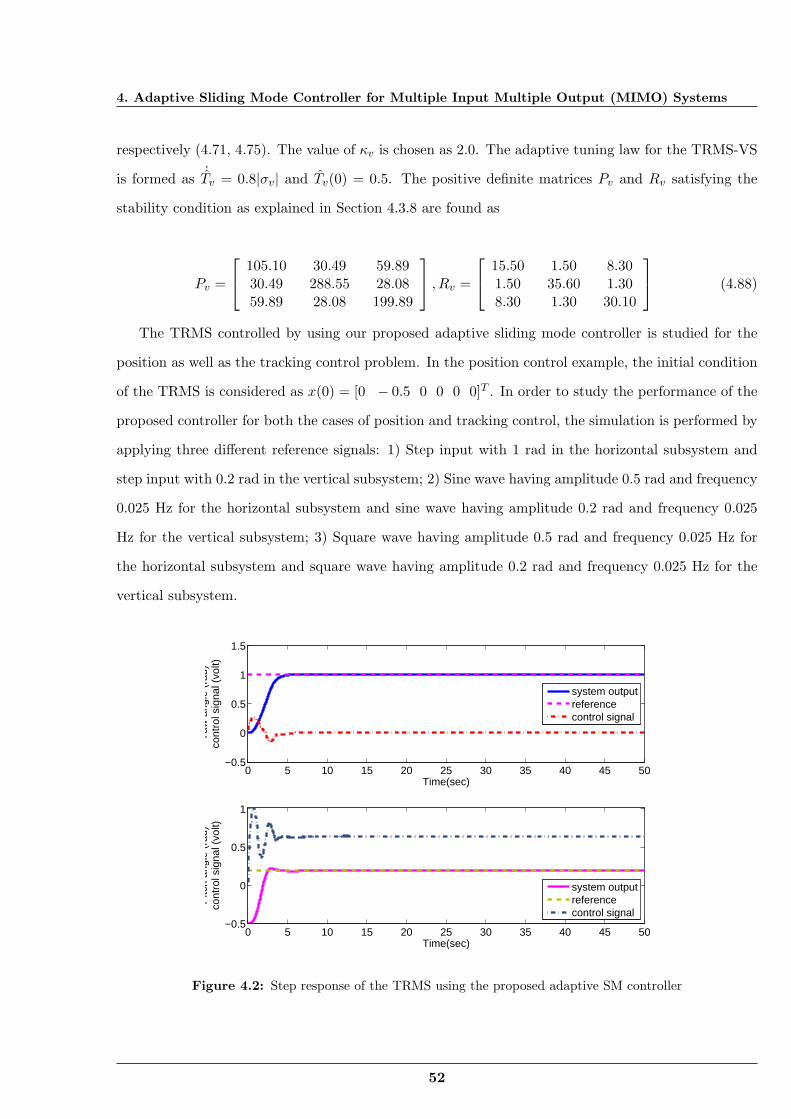
4. Adaptive Sliding Mode Controller for Multiple Input Multiple Output (MIMO) Systems
respectively (4.71, 4.75). The value of κv is chosen as 2.0. The adaptive tuning law for the TRMS-VS
is formed as ˙Tv = 0.8|σv| and Tv(0) = 0.5. The positive definite matrices Pv and Rv satisfying the
stability condition as explained in Section 4.3.8 are found as
Pv =
105.10 30.49 59.8930.49 288.55 28.0859.89 28.08 199.89
, Rv =
15.50 1.50 8.301.50 35.60 1.308.30 1.30 30.10
(4.88)
The TRMS controlled by using our proposed adaptive sliding mode controller is studied for the
position as well as the tracking control problem. In the position control example, the initial condition
of the TRMS is considered as x(0) = [0 − 0.5 0 0 0 0]T . In order to study the performance of the
proposed controller for both the cases of position and tracking control, the simulation is performed by
applying three different reference signals: 1) Step input with 1 rad in the horizontal subsystem and
step input with 0.2 rad in the vertical subsystem; 2) Sine wave having amplitude 0.5 rad and frequency
0.025 Hz for the horizontal subsystem and sine wave having amplitude 0.2 rad and frequency 0.025
Hz for the vertical subsystem; 3) Square wave having amplitude 0.5 rad and frequency 0.025 Hz for
the horizontal subsystem and square wave having amplitude 0.2 rad and frequency 0.025 Hz for the
vertical subsystem.
0 5 10 15 20 25 30 35 40 45 50−0.5
0
0.5
1
1.5
Time(sec)
Yaw
ang
le (
rad)
cont
rol s
igna
l (vo
lt)
system outputreferencecontrol signal
0 5 10 15 20 25 30 35 40 45 50−0.5
0
0.5
1
Time(sec)
Pitc
h an
gle
(rad
)co
ntro
l sig
nal (
volt)
system outputreferencecontrol signal
Figure 4.2: Step response of the TRMS using the proposed adaptive SM controller
52
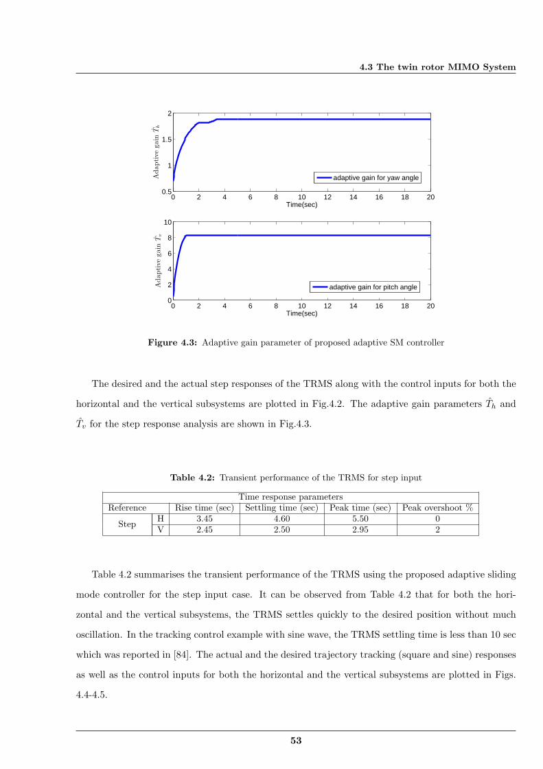
4.3 The twin rotor MIMO System
0 2 4 6 8 10 12 14 16 18 200.5
1
1.5
2
Time(sec)
Adaptive
gain
Th
adaptive gain for yaw angle
0 2 4 6 8 10 12 14 16 18 200
2
4
6
8
10
Time(sec)
Adaptive
gain
Tv
adaptive gain for pitch angle
Figure 4.3: Adaptive gain parameter of proposed adaptive SM controller
The desired and the actual step responses of the TRMS along with the control inputs for both the
horizontal and the vertical subsystems are plotted in Fig.4.2. The adaptive gain parameters Th and
Tv for the step response analysis are shown in Fig.4.3.
Table 4.2: Transient performance of the TRMS for step input
Time response parametersReference Rise time (sec) Settling time (sec) Peak time (sec) Peak overshoot %
Step H 3.45 4.60 5.50 0V 2.45 2.50 2.95 2
Table 4.2 summarises the transient performance of the TRMS using the proposed adaptive sliding
mode controller for the step input case. It can be observed from Table 4.2 that for both the hori-
zontal and the vertical subsystems, the TRMS settles quickly to the desired position without much
oscillation. In the tracking control example with sine wave, the TRMS settling time is less than 10 sec
which was reported in [84]. The actual and the desired trajectory tracking (square and sine) responses
as well as the control inputs for both the horizontal and the vertical subsystems are plotted in Figs.
4.4-4.5.
53
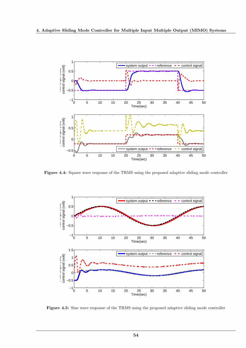
4. Adaptive Sliding Mode Controller for Multiple Input Multiple Output (MIMO) Systems
0 5 10 15 20 25 30 35 40 45 50−1
−0.5
0
0.5
1
Time(sec)
Yaw
ang
le (
rad)
con
trol
sig
nal (
volt)
system output reference control signal
0 5 10 15 20 25 30 35 40 45 50−0.5
0
0.5
1
Time(sec)
Pitc
h an
gle
(rad
) c
ontr
ol s
igna
l (vo
lt)
system output reference control signal
Figure 4.4: Square wave response of the TRMS using the proposed adaptive sliding mode controller
0 5 10 15 20 25 30 35 40 45 50−1
−0.5
0
0.5
1
Time(sec)
Yaw
ang
le (
rad)
con
trol
sig
nal (
volt)
system output reference control signal
0 5 10 15 20 25 30 35 40 45 50−1
−0.5
0
0.5
1
1.5
Time(sec)
Pitc
h an
gle
(rad
) c
ontr
ol s
igna
l (vo
lt)
system output reference control signal
Figure 4.5: Sine wave response of the TRMS using the proposed adaptive sliding mode controller
54
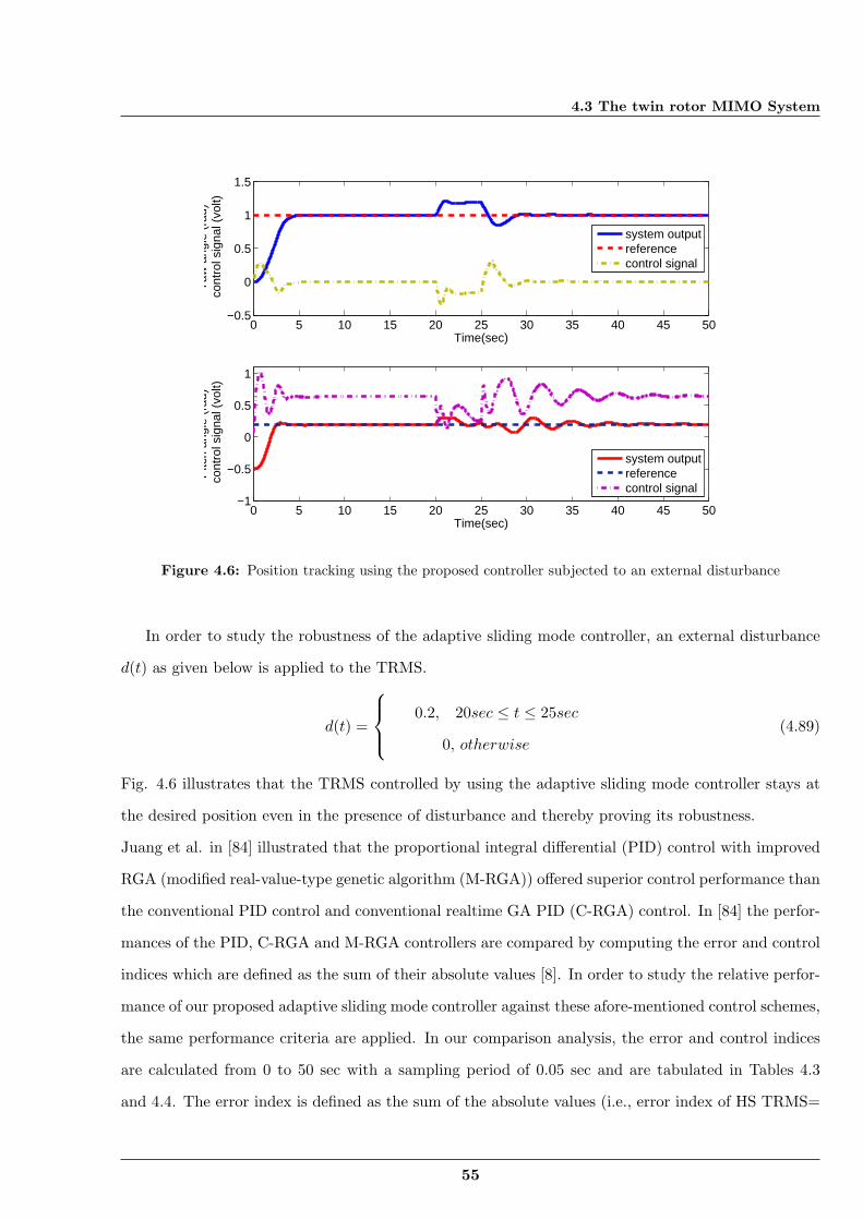
4.3 The twin rotor MIMO System
0 5 10 15 20 25 30 35 40 45 50−0.5
0
0.5
1
1.5
Time(sec)
Yaw
ang
le (
rad)
con
trol
sig
nal (
volt)
system outputreferencecontrol signal
0 5 10 15 20 25 30 35 40 45 50−1
−0.5
0
0.5
1
Time(sec)
Pitc
h an
gle
(rad
) c
ontr
ol s
igna
l (vo
lt)
system outputreferencecontrol signal
Figure 4.6: Position tracking using the proposed controller subjected to an external disturbance
In order to study the robustness of the adaptive sliding mode controller, an external disturbance
d(t) as given below is applied to the TRMS.
d(t) =
0.2, 20sec ≤ t ≤ 25sec
0, otherwise(4.89)
Fig. 4.6 illustrates that the TRMS controlled by using the adaptive sliding mode controller stays at
the desired position even in the presence of disturbance and thereby proving its robustness.
Juang et al. in [84] illustrated that the proportional integral differential (PID) control with improved
RGA (modified real-value-type genetic algorithm (M-RGA)) offered superior control performance than
the conventional PID control and conventional realtime GA PID (C-RGA) control. In [84] the perfor-
mances of the PID, C-RGA and M-RGA controllers are compared by computing the error and control
indices which are defined as the sum of their absolute values [8]. In order to study the relative perfor-
mance of our proposed adaptive sliding mode controller against these afore-mentioned control schemes,
the same performance criteria are applied. In our comparison analysis, the error and control indices
are calculated from 0 to 50 sec with a sampling period of 0.05 sec and are tabulated in Tables 4.3
and 4.4. The error index is defined as the sum of the absolute values (i.e., error index of HS TRMS=
55
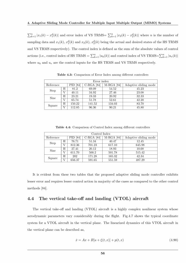
4. Adaptive Sliding Mode Controller for Multiple Input Multiple Output (MIMO) Systems
∑nk=1 |x1(k) − xd1(k)| and error index of VS TRMS=
∑nk=1 |x2(k) − xd2(k)| where n is the number of
sampling data and x1(k), xd1(k) and x2(k), xd2(k) being the actual and desired states of the HS TRMS
and VS TRMS respectively). The control index is defined as the sum of the absolute values of control
actions (i.e., control index of HS TRMS =∑n
k=1 |uh(k)| and control index of VS TRMS=∑n
k=1 |uv(k)|
where uh and uv are the control inputs for the HS TRMS and VS TRMS respectively.
Table 4.3: Comparison of Error Index among different controllers
Error indexReference PID [84] C-RGA [84] M-RGA [84] Adaptive sliding mode
Step H 81.2 69.09 54.52 45.23V 40.11 34.92 27.46 23.08
Sine H 23.21 19.33 20.92 32.33V 65.74 51.78 52.61 42.20
Square H 150.22 141.52 134.03 83.70V 112.85 96.36 90.21 45.80
Table 4.4: Comparison of Control Index among different controllers
Control IndexReference PID [84] C-RGA [84] M-RGA [84] Adaptive sliding mode
Step H 76.71 51.34 40.47 12.45V 812.36 701.23 617.10 645.98
Sine H 27.41 20.12 18.93 10.68V 611.70 500.2 501.78 515.42
Square H 202 171.28 165.32 42.34V 656.37 591.65 551.59 487.29
It is evident from these two tables that the proposed adaptive sliding mode controller exhibits
lesser error and requires lesser control action in majority of the cases as compared to the other control
methods [84].
4.4 The vertical take-off and landing (VTOL) aircraft
The vertical take-off and landing (VTOL) aircraft is a highly complex nonlinear system whose
aerodynamic parameters vary considerably during the flight. Fig.4.7 shows the typical coordinate
system for a VTOL aircraft in the vertical plane. The linearized dynamics of this VTOL aircraft in
the vertical plane can be described as,
x = Ax+B[u+ ξ(t, x)] + p(t, x) (4.90)
56
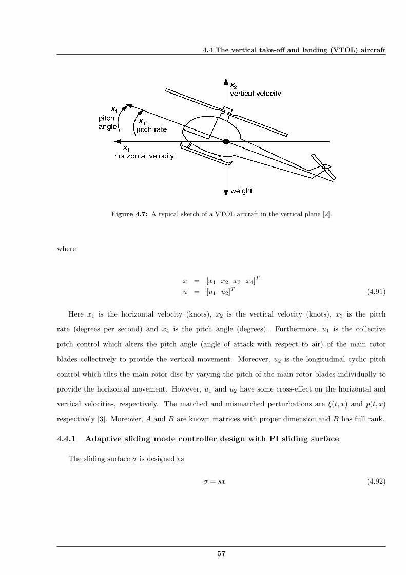
4.4 The vertical take-off and landing (VTOL) aircraft
Figure 4.7: A typical sketch of a VTOL aircraft in the vertical plane [2].
where
x = [x1 x2 x3 x4]T
u = [u1 u2]T (4.91)
Here x1 is the horizontal velocity (knots), x2 is the vertical velocity (knots), x3 is the pitch
rate (degrees per second) and x4 is the pitch angle (degrees). Furthermore, u1 is the collective
pitch control which alters the pitch angle (angle of attack with respect to air) of the main rotor
blades collectively to provide the vertical movement. Moreover, u2 is the longitudinal cyclic pitch
control which tilts the main rotor disc by varying the pitch of the main rotor blades individually to
provide the horizontal movement. However, u1 and u2 have some cross-effect on the horizontal and
vertical velocities, respectively. The matched and mismatched perturbations are ξ(t, x) and p(t, x)
respectively [3]. Moreover, A and B are known matrices with proper dimension and B has full rank.
4.4.1 Adaptive sliding mode controller design with PI sliding surface
The sliding surface σ is designed as
σ = sx (4.92)
57
4. Adaptive Sliding Mode Controller for Multiple Input Multiple Output (MIMO) Systems
where s ∈ Rm∗n is a constant matrix designed by selecting the eigen values suitably (all negative)
to make the system stable [68]. By using the transformation [3] [35] [86]
z
σ
= Mx where the
transformation matrix
M =
Wg
Bg
, Eq.(4.90) can be transformed to
z = WgAWz +WgABσ +Wgp(t, x)
σ = BgAWz +BgABσ + u+ ξ(t, x) + sp(t, x) (4.93)
Here s = Bg and Wg, Bg satisfy BgB = Im, BgW = 0, WgB = 0, and WgW = In−m. The matrix
W is chosen in such a way that J = WgAW has the desired eigen values [86] where J is a symmetric
matrix. It can be verified that
M−1 = [W B] (4.94)
When the system is in the sliding mode, it satisfies the conditions σ = 0 and σ = 0. Then the
perturbation term in Eq.(4.93) becomes Wgp(t, x) = Wgp(t,Wz) = pr(t, z). Now the reduced order
equation becomes
z = Jz + pr(t, z) (4.95)
If the mismatched perturbation pr(t, z) satisfies ||pr(t, z)|| ≤ ϕr||z|| where ϕr < −λmax(J), λmax(J)
being the maximum eigen value of the J matrix, then by choosing the Lyapunov function V = 12 ||z||
2,
it can be proved that [3] [38]
V = zTJz + zT pr(t, z) ≤ λmax(J)||z||2 + ϕr||z||2 = [λmax(J) + ϕr]V < 0 (4.96)
The above condition means that the system will be asymptotically stable once the sliding mode is
reached. However, it is obvious from the above discussion that the sliding surface design requires the
bounds of the uncertainties to be known apriori [75] which is extremely difficult practically. Hence
the need arises for designing the sliding surface in such a way that prior knowledge about the bounds
of the uncertainties is not required.
58
4.4 The vertical take-off and landing (VTOL) aircraft
4.4.2 The adaptive PI sliding surface design
Let us consider the sliding surface
σ = s(t)x (4.97)
The sliding coefficient matrix s(t) ∈ Rm∗n can be designed as [3]
s(t) = B+ +N(t)Wg (4.98)
where B+ = (BTB)−1BT ∈ Rm∗n is the Moore-Penrose pseudo inverse [20] of B and N(t) ∈ Rm∗n is
designed using adaptive technique to be explained later. Let us consider the transformation z
σ
=
Wg
s(t)
x = M(t)x (4.99)
Now defining W (t) = W+g − BN(t) ∈ Rn∗(n−m) and W+
g = W Tg (WgW
Tg )−1 ∈ Rn∗(n−m), it can be
verified that
M(t)−1 = [W (t) B] (4.100)
From Eq.s (4.99) and (4.100), it can be observed that
x = W (t)z +Bσ (4.101)
So, Eq.(4.90) gets transformed to
z = WgAW (t)z +WgABσ +Wgp(t, x) (4.102)
σ = s(t)AW (t)z + s(t)ABσ + u+ N(t)z + ξ(t, x) + s(t)p(t, x) (4.103)
When the system is in the sliding mode, it satisfies the conditions σ = 0 and σ = 0. Then the per-
turbation term in Eq.(4.102) becomes Wgp(t, x) = Wgp(t,W (t)z) = p(t, z) and Eq.(4.102) transforms
into a reduced order equation as,
z = Az + Bv(t) + p(t, z) (4.104)
59
4. Adaptive Sliding Mode Controller for Multiple Input Multiple Output (MIMO) Systems
where A = WgAW+g ∈ R(n−m)∗(n−m), B = WgAB ∈ R(n−m)∗m and v(t) = −N(t)z ∈ Rm.
Theorem 4.1. Let us consider the perturbed dynamic equation (4.104) under the assumption that
n ≤ 2m. Suppose that B has full rank and the mismatched perturbations in the domain of interest
satisfy ∥p(t, z)∥ ≤ ϕ2||z||, where ϕ2 is an unknown positive constant. If the feedback gain N(t) of the
controller is designed as [38]
N(t) = K2 + [ϕ2(t) + ρ]B+ (4.105)
where ρ is a positive constant, K2 = B+A , B+ = BT (BBT )−1 ∈ Rm∗(n−m) and ϕ2(t) is an adaptive
gain given by
ϕ2(t) =∫ t
t0
θ||z||2dτ + ϕ2(t0) (4.106)
with θ > 0 being a positive constant and ϕ2(t0) = 0 being the initial condition, then ϕ2(t) is bounded
and the trajectories z (4.104) and state x will be asymptotically stable in the sliding mode.
Proof. Let us consider the Lyapunov function V2(z, ϕ2) = 12 [∥z∥2 + θ−1ϕ2(t)2]. Here ϕ2(t) is the
estimation error of the adaptive gain given by ϕ2(t) = ϕ2(t) − ϕ2(t), where ϕ2(t) is the estimated
adaptive gain and ϕ2(t) is the actual adaptive gain [3]. Then
V2(z, ϕ2) = zT Az + zT Bv + zT p+ θ−1ϕ2˙ϕ2
≤ zT Az + zT Bv + ||z||||p|| + θ−1ϕ2˙ϕ2
≤ zT Az + zT Bv + ϕ2||z||2 + (ϕ2 − ϕ2)||z||2
≤ zT Az + zT Bv + ϕ2||z||2
≤ −ρ||z||2 ≤ 0 (4.107)
It is obvious from the above discussion that z ∈ L2 ∩ L∞ and ϕ2(t) ∈ L∞. Hence from Eq.s (4.104),
(4.105) and the fact that ∥p(t, z)∥ ≤ ϕ2 ∥z∥, it can be shown that z ∈ L∞ as well as V2 ∈ L∞.
From Barbalat’s lemma [30], it is found that z → 0 as t → ∞. The bound of the adaptation law is
0 ≤ ϕ2(t) ≤ (∥z(t0)∥2 + ϕ22)/ρ. Moreover, it can be seen from equation (4.105) that N(t) is bounded
since ϕ2(t) ∈ L∞ and hence the state x(t) = W (t)z = [W+g −BN(t)]z becomes asymptotically stable
as the system reaches the sliding mode.
It can be observed in Fig.4.7 that the VTOL weighs asymmetrically as the main propeller is heavier
than the tail propeller, i.e. the horizontal velocity and the vertical velocity would not stay in the
60
4.4 The vertical take-off and landing (VTOL) aircraft
desired states because of gravity. As such, control performance of the VTOL tends to be poor. In
order to eliminate the effect of the asymmetrical weight and reduce the offset in control, a proportional
plus integral sliding surface is used in the proposed controller. The sliding surface is chosen as,
σ′ = s(t)x−B+(A+BK)∫ t
0xdτ (4.108)
where x is the state vector and B+ = (BTB)−1BT ∈ Rm∗n is the the Moore-Penrose pseudo inverse
of B [20]. Moreover, K is the design matrix ∈ Rm∗n to satisfy the inequality
Re[λmax(A+BK) < 0] (4.109)
Taking the derivative of σ′ and using (4.103) yields
σ′ = s(t)AW (t)z + s(t)ABσ + u−B+(A+BK)(W (t)z +Bσ) + d(t, x) (4.110)
where,
d(t, x) = N(t)z + ξ(t, x) + s(t)p(t, x)
= θ ∥Wgx∥2 B+Wgx+ ξ(t, x) + s(t)p(t, x) (4.111)
The second derivative of σ′ can be expressed as
σ′ = s(t)AW (t)z + s(t)AW (t)z + s(t)AW (t)z + s(t)ABσ + s(t)ABσ
−B+(A+BK)(W (t)z +W (t)z +Bσ) + u+ d(t, x) (4.112)
In the above equation (4.112), d(t, x) is considered as unknown disturbance or perturbation.
Assumption 4.1.: The disturbance d(t, x) in (4.112) is assumed to be bounded and satisfy the
following condition:
||d(t, x)|| ≤r∑i=0
Bi||x||i (4.113)
where Bi are unknown bounds, which are not easily obtained due to the complicated structure of the
uncertainties in practical control systems. Furthermore, r is a positive integer determined by the
designer in accordance with the knowledge about the order of the perturbations. For example, if the
perturbations contain a term x31, then one may choose r = 3. However, if x4
1 exists in the perturbation,
then the inequality might not be satisfied for certain domain of x if one still chooses r = 3 [38].
61
4. Adaptive Sliding Mode Controller for Multiple Input Multiple Output (MIMO) Systems
Let us define the sliding manifold l(t) such that,
l(t) = σ′ + κσ′
l(t) = σ′ + κσ′ (4.114)
Using the above equations (4.112), (4.113) and (4.114) yields
l(t) = s(t)AW (t)z + s(t)AW (t)z + s(t)AW (t)z + s(t)ABσ + s(t)ABσ
−B+(A+BK)(W (t)z +W (t)z +Bσ) + u+ d(t, x) + κσ′ (4.115)
The derivative of the sliding manifold l(t) can be expressed as
l(t) = Φ(t, z, u) + ψ(t, z)u (4.116)
where Φ(t, z, u) = s(t)AW (t)z+s(t)AW (t)z+s(t)AW (t)z+s(t)ABσ+s(t)ABσ−B+(A+BK)(W (t)z+
W (t)z + Bσ) + d(t, x) + κσ′ collects all the uncertain terms not involving u and ψ(t, z) = 1. From
equation (4.115), the equivalent control ueq for controlling the nominal system can be designed as
ueq = −[s(t)AW (t)z + s(t)AW (t)z + s(t)AW (t)z + s(t)ABσ
+s(t)ABσ −B+(A+BK)(W (t)z +W (t)z +Bσ) + κσ′] if l(t) = 0
= 0 otherwise (4.117)
In practice, the bounds of the system uncertainty are often unknown in advance and hence the error
term d(t, x) in equation (4.112) is difficult to find. So an adaptive tuning law is proposed to estimate
d(t, x). Now the proposed adaptive controller for tackling the system uncertainty is designed as [87],
uadp = −r∑i=0
ˆBi||x||isign(l(t)) if l(t) = 0
= 0 otherwise (4.118)
where ˆBi is the adaptive parameter which is tuned using the following adaptive rule,
˙Bi = −θiρi ˆBi + θi||l(t)||||x||i if l(t) = 0
= 0 otherwise (4.119)
62
4.4 The vertical take-off and landing (VTOL) aircraft
where ρi and θi are positive constants, ˆBi(0) = 0 is the initial condition, 0 ≤ i ≤ r.
The switching control law us can be designed as,
us = −τ l(t) − ηsign(l(t)) if l(t) = 0
= 0 otherwise (4.120)
where τ and η are positive constants.
Now the control law u can be obtained as,
u = ueq + uadp + us (4.121)
where ueq is the equivalent control part, uadp is the adaptive control part and us is the switching
control.
Theorem 4.2. Let us consider the system (4.90) with the adaptive sliding surface given by (4.98)
and (4.105). The trajectory of the closed loop system (4.90) can be driven onto the sliding manifold
l(t) in finite time by using the controller given by
u = −[s(t)AW (t)z + s(t)AW (t)z + s(t)AW (t)z + s(t)ABσ
+s(t)ABσ −B+(A+BK)(W (t)z +W (t)z +Bσ) + κσ′]
−r∑i=0
ˆBi||x||isign(l(t)) − τ l(t) − ηsign(l(t)) if l(t) = 0
= 0 otherwise (4.122)
Proof. Let us define a Lyapunov function V0 as follows [40,87],
V0 =12l(t)T l(t) +
12
r∑i=0
θ−1i
˜B2i (4.123)
where ˜Bi(t) = ˆBi(t)− Bi are the estimation errors of the adaptive gains. The time derivative of V0 is
obtained as,
V0 = l(t)T l(t) +r∑i=0
θ−1i
˜Bi˙Bi
= l(t)T [s(t)AW (t)z + s(t)AW (t)z + s(t)AW (t)z + s(t)ABσ
+s(t)ABσ −B+(A+BK)(W (t)z +W (t)z +Bσ) + κσ′ + u+ d(t, x)] +r∑i=0
θ−1i
˜Bi
63
4. Adaptive Sliding Mode Controller for Multiple Input Multiple Output (MIMO) Systems
= l(t)T [s(t)AW (t)z + s(t)AW (t)z + s(t)AW (t)z + s(t)ABσ
+s(t)ABσ −B+(A+BK)(W (t)z +W (t)z +Bσ) + κσ′ + u+ d(t, x)]
+r∑i=0
θ−1i ( ˆBi(t) − Bi)θi(−ρi ˆBi + ||l(t)|| ∥x∥i)
Using the relations in (4.117-4.120) yields,
V0 ≤ [−r∑i=0
ˆBi||x||i||l(t)|| −r∑i=0
Bi||x||i||l(t)|| − τ ||l(t)|| − η||l(t)||
+r∑i=0
ˆBi||x||i||l(t)|| +r∑i=0
Bi||x||i||l(t)||] − ρi( ˆB2i − ˆBiBi)
≤ −ηl(t)sign(l(t)) − τ l(t)2 − ρi( ˆBi −12Bi)2 +
14ρiB
2i
≤ −η||l(t)|| − τ l(t)2 +14ρiB
2i (4.124)
It is clear that V0 < 0 if l(t) >√
δ14τmin
or ||l(t)|| > δ14ηmin
, where η, τ are positive design parameters
and δ1 = ρiB2i . The decrease of V0 eventually drives the trajectories of the closed loop system into
l(t) >√
δ14τmin
and ||l(t)|| > δ14ηmin
. Therefore, the trajectories of the closed loop system are bounded
ultimately as
limt→∞
l(t) ∈
(l(t) >
√δ1
4τmin
)∩(||l(t)|| > δ1
4ηmin
)(4.125)
which is a small set containing the origin of the closed loop system. In order to guarantee bounded
motion around the sliding surface, the positive parameters η and τ are chosen to be large enough such
that V0 < 0 when V0 is out of the bounded region which contains an equilibrium point [40]. It can
be observed that V0 < 0 is achievable which implies that the sliding manifold l(t) will approach zero
in finite time. Therefore, the control law given by (4.122) guarantees that the sliding mode will be
reached in finite time and sustained thereafter [87].
Remark 4.4. Once the sliding mode is established, the proposed gain adaptation law (4.119) allows
the gain ˆBi to decrease. Thus it is seen that the proposed gain adaptation law, while maintaining the
sliding mode, keeps the gain ˆBi at the smallest possible level to ensure accuracy.
Thus the adaptive gain tuning law is modified as,
˙Bi = −θiρi ˆBi + θi||l(t) − ℘||||x||i if l(t) = 0
= 0 otherwise (4.126)
64
4.4 The vertical take-off and landing (VTOL) aircraft
where 0 ≤ i ≤ r and ℘ is a small positive number.
Remark 4.5. The parameter τ in the controller (4.122) is very crucial as it is one of the parameters
responsible for determining the convergence rate of the sliding surface. It is clear that a large value of
τ will force the system states to converge to the origin at a high speed. Since a high η will require a
very high control input which is not desirable in reality, the parameter η cannot be selected too large.
Hence a compromise has to be made between the response speed and the control input.
Remark 4.6. The parameters ρ0 and ρ1 in (4.126) determine the convergence rate of the estimated
bounds ˆB0 and ˆB1. Large values of ρ0 and ρ1 can be chosen so that the estimated bounds ˆB0 and ˆB1
converge quickly to the actual bounds.
4.4.3 Effectiveness
Let us compare the proposed adaptive sliding mode controller with the adaptive sliding mode
controller (SMC) designed by Wen and Cheng [3] and given below:
u = uf + uadp + us (4.127)
where
uf = −s(t)AW (t)z − s(t)ABσ
uadp = −r∑i=0
ˆBi||x||iσ
||σ||if σ = 0
= 0 otherwise
us = −η σ
||σ||if σ = 0
= 0 otherwise
(4.128)
The adaptive parameter ˆBi is tuned using the following adaptive rule,
˙Bi = θi||x||i if σ = 0
= 0 otherwise
(4.129)
where θi are positive constants, ˆBi(0) = 0 is the initial condition, 0 ≤ i ≤ r.
Implementation of the adaptive SMC (4.127-4.129) is limited by the obvious drawback of the gain ˆBi
65
4. Adaptive Sliding Mode Controller for Multiple Input Multiple Output (MIMO) Systems
being susceptible to overestimation and thereby increasing the chattering in the system. Furthermore,
this approach is not directly applicable to real systems but requires modifications involving the sign
function which needs replacement by a saturation function. However, the width of the boundary layer
in the saturation function affects accuracy and robustness of the SMC. Furthermore, no methodology
for tuning the boundary layer width is provided in [3].
4.4.4 Simulation Results
The typical load and flight conditions for the VTOL aircraft are considered at the nominal airspeed
of 135 knots [3]. The linearized dynamics of this VTOL aircraft in the vertical plane can be described
by (4.90 - 4.91) where,
A =
−0.0366 0.0271 0.0188 −0.45550.0482 −1.0100 0.0024 −4.02080.1002 0.3681 −0.7070 1.4200
0 0 1 0
, B =
−0.4422 0.17613.5446 −7.5922−5.52 4.49
0 0
ξ(t, x) =[
−5 sin(0.5t) + x3
2 cos(0.2x1)x2 + 3
], p(t, x) =
sin(0.1x2)(0.1x3 + 0.7x4)
−0.3x4 cos(0.3x4t)−2x1 − 0.3x2
(0.2x1 + 0.4x4) sin(0.4x3)
(4.130)
The simulation is carried out in MATLAB Simulink platform by using ODE 4 solver with a fixed
step size of 0.001sec. The reference vector is chosen as xd = [0 0 0 0]T since all the states are to be
driven to zero. For comparison purpose, the associated design parameters of the proposed adaptive
sliding mode controller are chosen following [3]. As such Wg is selected as,
Wg =
0.0666 0.0076 0.0102 0.72
0.8879 0.1010 0.136 −0.028
(4.131)
Hence WgB = 0 [86]. Next the pseudo control input, the adaptive controller and the adaptive gains
are designed in accordance with equations (4.105), (4.106), (4.119) and (4.126) where θ = 0.1474,
θ0 = 0.1271, θ1 = 0.1251, ρ = 0.1971, η = 2, τ = 1, κ = diag(1.25, 1.25), ρ = 0.1519 and K is so
chosen that the eigen values are placed at −0.5,−0.7,−15,−25 [20]. The initial state is assumed as
x(0) = [2 − 2 1 1]T .
66
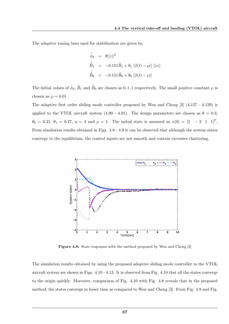
4.4 The vertical take-off and landing (VTOL) aircraft
The adaptive tuning laws used for stabilization are given by,
˙ϕ2 = θ||z||2
˙B1 = −0.151 ˆB1 + θ1 ||l(t) − ℘|| ||x||˙B0 = −0.151 ˆB0 + θ0 ||l(t) − ℘||
The initial values of ϕ2, ˆB1 and ˆB0 are chosen as 0, 1, 1 respectively. The small positive constant ℘ is
chosen as ℘ = 0.01.
The adaptive first order sliding mode controller proposed by Wen and Cheng [3] (4.127 - 4.129) is
applied to the VTOL aircraft system (4.90 - 4.91). The design parameters are chosen as θ = 0.3,
θ0 = 0.21, θ1 = 0.27, η = 4 and ρ = 1. The initial state is assumed as x(0) = [2 − 2 1 1]T .
From simulation results obtained in Figs. 4.8 - 4.9 it can be observed that although the system states
converge to the equilibrium, the control inputs are not smooth and contain excessive chattering.
0 1 2 3 4 5 6 7 8 9 10−4
−3
−2
−1
0
1
2
3
Time(sec)
Sys
tem
sta
tes
x1
x2
x3
x4
Figure 4.8: State responses with the method proposed by Wen and Cheng [3]
The simulation results obtained by using the proposed adaptive sliding mode controller to the VTOL
aircraft system are shown in Figs. 4.10 - 4.13. It is observed from Fig. 4.10 that all the states converge
to the origin quickly. Moreover, comparison of Fig. 4.10 with Fig. 4.8 reveals that in the proposed
method, the states converge in lesser time as compared to Wen and Cheng [3]. From Fig. 4.9 and Fig.
67
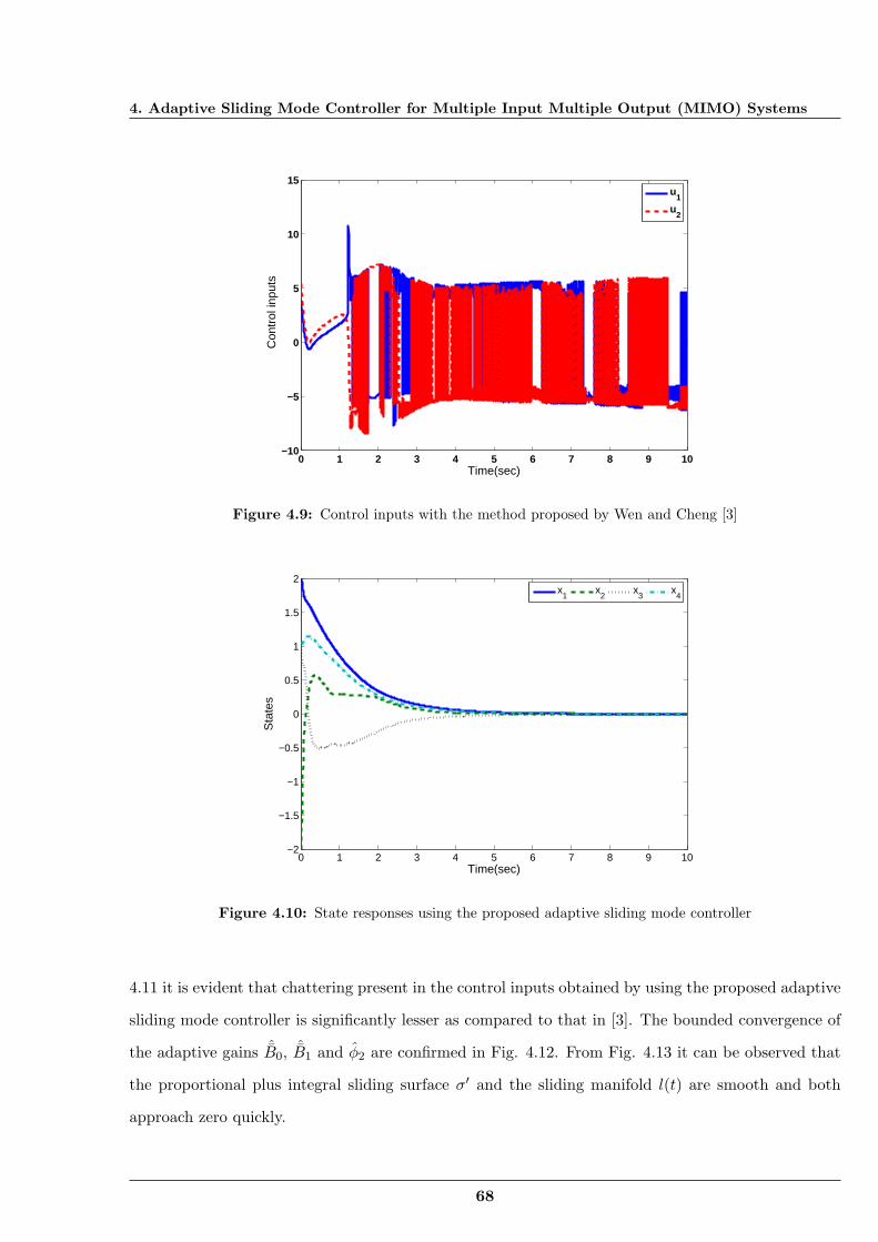
4. Adaptive Sliding Mode Controller for Multiple Input Multiple Output (MIMO) Systems
0 1 2 3 4 5 6 7 8 9 10−10
−5
0
5
10
15
Time(sec)
Con
trol
inpu
ts
u1
u2
Figure 4.9: Control inputs with the method proposed by Wen and Cheng [3]
0 1 2 3 4 5 6 7 8 9 10−2
−1.5
−1
−0.5
0
0.5
1
1.5
2
Time(sec)
Sta
tes
x1
x2
x3
x4
Figure 4.10: State responses using the proposed adaptive sliding mode controller
4.11 it is evident that chattering present in the control inputs obtained by using the proposed adaptive
sliding mode controller is significantly lesser as compared to that in [3]. The bounded convergence of
the adaptive gains ˆB0, ˆB1 and ϕ2 are confirmed in Fig. 4.12. From Fig. 4.13 it can be observed that
the proportional plus integral sliding surface σ′ and the sliding manifold l(t) are smooth and both
approach zero quickly.
68
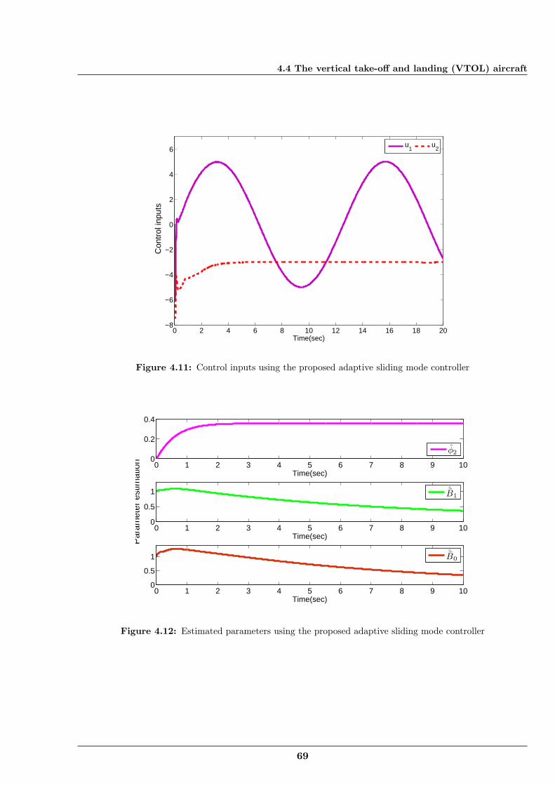
4.4 The vertical take-off and landing (VTOL) aircraft
0 2 4 6 8 10 12 14 16 18 20−8
−6
−4
−2
0
2
4
6
Time(sec)
Con
trol
inpu
ts
u1
u2
Figure 4.11: Control inputs using the proposed adaptive sliding mode controller
0 1 2 3 4 5 6 7 8 9 100
0.2
0.4
Time(sec)
φ2
0 1 2 3 4 5 6 7 8 9 100
0.5
1
Time(sec)
Par
amet
er e
stim
atio
n
ˆB1
0 1 2 3 4 5 6 7 8 9 100
0.5
1
Time(sec)
ˆB0
Figure 4.12: Estimated parameters using the proposed adaptive sliding mode controller
69
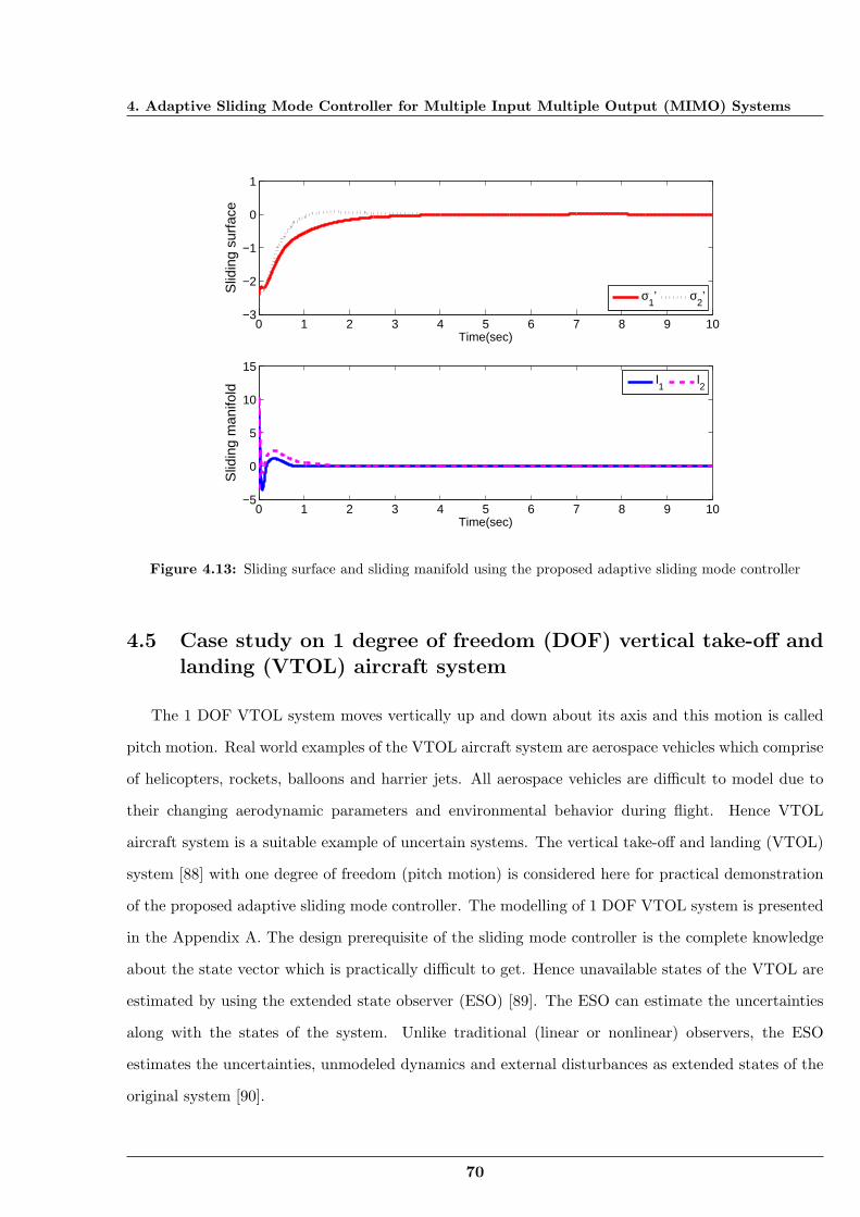
4. Adaptive Sliding Mode Controller for Multiple Input Multiple Output (MIMO) Systems
0 1 2 3 4 5 6 7 8 9 10−3
−2
−1
0
1
Time(sec)
Slid
ing
surf
ace
σ1’ σ
2’
0 1 2 3 4 5 6 7 8 9 10−5
0
5
10
15
Time(sec)
Slid
ing
man
ifold
l1
l2
Figure 4.13: Sliding surface and sliding manifold using the proposed adaptive sliding mode controller
4.5 Case study on 1 degree of freedom (DOF) vertical take-off andlanding (VTOL) aircraft system
The 1 DOF VTOL system moves vertically up and down about its axis and this motion is called
pitch motion. Real world examples of the VTOL aircraft system are aerospace vehicles which comprise
of helicopters, rockets, balloons and harrier jets. All aerospace vehicles are difficult to model due to
their changing aerodynamic parameters and environmental behavior during flight. Hence VTOL
aircraft system is a suitable example of uncertain systems. The vertical take-off and landing (VTOL)
system [88] with one degree of freedom (pitch motion) is considered here for practical demonstration
of the proposed adaptive sliding mode controller. The modelling of 1 DOF VTOL system is presented
in the Appendix A. The design prerequisite of the sliding mode controller is the complete knowledge
about the state vector which is practically difficult to get. Hence unavailable states of the VTOL are
estimated by using the extended state observer (ESO) [89]. The ESO can estimate the uncertainties
along with the states of the system. Unlike traditional (linear or nonlinear) observers, the ESO
estimates the uncertainties, unmodeled dynamics and external disturbances as extended states of the
original system [90].
70
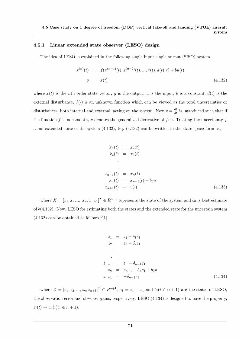
4.5 Case study on 1 degree of freedom (DOF) vertical take-off and landing (VTOL) aircraftsystem
4.5.1 Linear extended state observer (LESO) design
The idea of LESO is explained in the following single input single output (SISO) system,
x(n)(t) = f(x(n−1)(t), x(n−2)(t), ..., x(t), d(t), t) + bu(t)
y = x(t) (4.132)
where x(t) is the nth order state vector, y is the output, u is the input, b is a constant, d(t) is the
external disturbance, f(·) is an unknown function which can be viewed as the total uncertainties or
disturbances, both internal and external, acting on the system. Now v = dfdt is introduced such that if
the function f is nonsmooth, v denotes the generalized derivative of f(·). Treating the uncertainty f
as an extended state of the system (4.132), Eq. (4.132) can be written in the state space form as,
x1(t) = x2(t)x2(t) = x3(t)
.
.
xn−1(t) = xn(t)xn(t) = xn+1(t) + b0u
xn+1(t) = v(·) (4.133)
where X = [x1, x2, ..., xn, xn+1]T ∈ Rn+1 represents the state of the system and b0 is best estimate
of b(4.132). Now, LESO for estimating both the states and the extended state for the uncertain system
(4.132) can be obtained as follows [91]
z1 = z2 − δ1e1
z2 = z3 − δ2e1
.
.
zn−1 = zn − δn−1e1
zn = zn+1 − δne1 + b0u
zn+1 = −δn+1e1 (4.134)
where Z = [z1, z2, ..., zn, zn+1]T ∈ Rn+1, e1 = z1 − x1 and δi(i ∈ n + 1) are the states of LESO,
the observation error and observer gains, respectively. LESO (4.134) is designed to have the property,
zi(t) → xi(t)(i ∈ n+ 1).
71
4. Adaptive Sliding Mode Controller for Multiple Input Multiple Output (MIMO) Systems
Writing the extended order system (4.133) in the state space form gives rise to,
X = AX +Bu+ Ev (4.135)
where X = [x1, x2, ..., xn, xn+1]T is the state vector of the extended order system. Here A, B and
E matrices are given by,
A =
0 1 .... 0 00 0 1 .... 0..0 0 0 .... 10 0 0 .... 0
, B =
00..b00
, E =
00..01
(4.136)
So (4.134) represents LESO for the system (4.135). The state space model of the LESO dynamics
can be written as
Z = AZ +Bu+ L(y − CZ) (4.137)
where L = [δ1 δ2....δn δn+1]T is the observer gain vector, y is output vector and C = [1 0 0.....0] is
the output matrix.
The parameters are chosen in a special way as sn+1 +δ1sn+ ....+δn+1 = (s+ω0)n+1, where ω0 denotes
the bandwidth of the LESO (4.134) [92]. It is proved that if f is differentiable with respect to t and
v = f is bounded, then the LESO (4.134) can estimate f(t) with bounded error and also estimates
the unknown states.
Remark 4.7. In the control law (4.22), the derivative term s is needed. However, in real time
implementation, direct differentiation will lead to erroneous result as the measurements are often
noisy. There are three methods to resolve this issue, namely, the derivative estimator, the suboptimal
algorithm and the twisting algorithm. In experimental study of the VTOL system, the first method is
utilized. A derivative estimator is designed using the method in [25] [64] and is given below,
z0 = −λ1|z0 − s|1/2sign(z0 − s) + z1
z1 = −λ2sign(z0 − s) (4.138)
where λ1 > 0 and λ2 > 0 are the design parameters and the estimators are designed as s = z1.
72
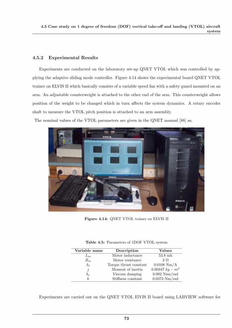
4.5 Case study on 1 degree of freedom (DOF) vertical take-off and landing (VTOL) aircraftsystem
4.5.2 Experimental Results
Experiments are conducted on the laboratory set-up QNET VTOL which was controlled by ap-
plying the adaptive sliding mode controller. Figure 4.14 shows the experimental board QNET VTOL
trainer on ELVIS II which basically consists of a variable speed fan with a safety guard mounted on an
arm. An adjustable counterweight is attached to the other end of the arm. This counterweight allows
position of the weight to be changed which in turn affects the system dynamics. A rotary encoder
shaft to measure the VTOL pitch position is attached to an arm assembly.
The nominal values of the VTOL parameters are given in the QNET manual [88] as,
Figure 4.14: QNET VTOL trainer on ELVIS II
Table 4.5: Parameters of 1DOF VTOL system
Variable name Description ValuesLm Motor inductance 53.8 mhRm Motor resistance 3 Ωkt Torque thrust constant 0.0108 Nm/Aj Moment of inertia 0.00347 kg −m2
bv Viscous damping 0.002 Nms/radk Stiffness constant 0.0373 Nm/rad
Experiments are carried out on the QNET VTOL ElVIS II board using LABVIEW software for
73
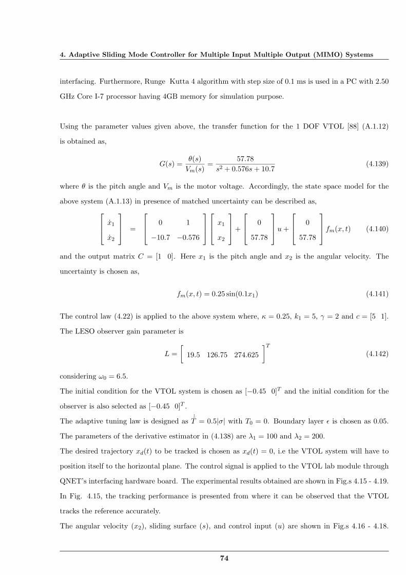
4. Adaptive Sliding Mode Controller for Multiple Input Multiple Output (MIMO) Systems
interfacing. Furthermore, Runge Kutta 4 algorithm with step size of 0.1 ms is used in a PC with 2.50
GHz Core I-7 processor having 4GB memory for simulation purpose.
Using the parameter values given above, the transfer function for the 1 DOF VTOL [88] (A.1.12)
is obtained as,
G(s) =θ(s)Vm(s)
=57.78
s2 + 0.576s+ 10.7(4.139)
where θ is the pitch angle and Vm is the motor voltage. Accordingly, the state space model for the
above system (A.1.13) in presence of matched uncertainty can be described as, x1
x2
=
0 1
−10.7 −0.576
x1
x2
+
0
57.78
u+
0
57.78
fm(x, t) (4.140)
and the output matrix C = [1 0]. Here x1 is the pitch angle and x2 is the angular velocity. The
uncertainty is chosen as,
fm(x, t) = 0.25 sin(0.1x1) (4.141)
The control law (4.22) is applied to the above system where, κ = 0.25, k1 = 5, γ = 2 and c = [5 1].
The LESO observer gain parameter is
L =[
19.5 126.75 274.625
]T(4.142)
considering ω0 = 6.5.
The initial condition for the VTOL system is chosen as [−0.45 0]T and the initial condition for the
observer is also selected as [−0.45 0]T .
The adaptive tuning law is designed as ˙T = 0.5|σ| with T0 = 0. Boundary layer ϵ is chosen as 0.05.
The parameters of the derivative estimator in (4.138) are λ1 = 100 and λ2 = 200.
The desired trajectory xd(t) to be tracked is chosen as xd(t) = 0, i.e the VTOL system will have to
position itself to the horizontal plane. The control signal is applied to the VTOL lab module through
QNET’s interfacing hardware board. The experimental results obtained are shown in Fig.s 4.15 - 4.19.
In Fig. 4.15, the tracking performance is presented from where it can be observed that the VTOL
tracks the reference accurately.
The angular velocity (x2), sliding surface (s), and control input (u) are shown in Fig.s 4.16 - 4.18.
74
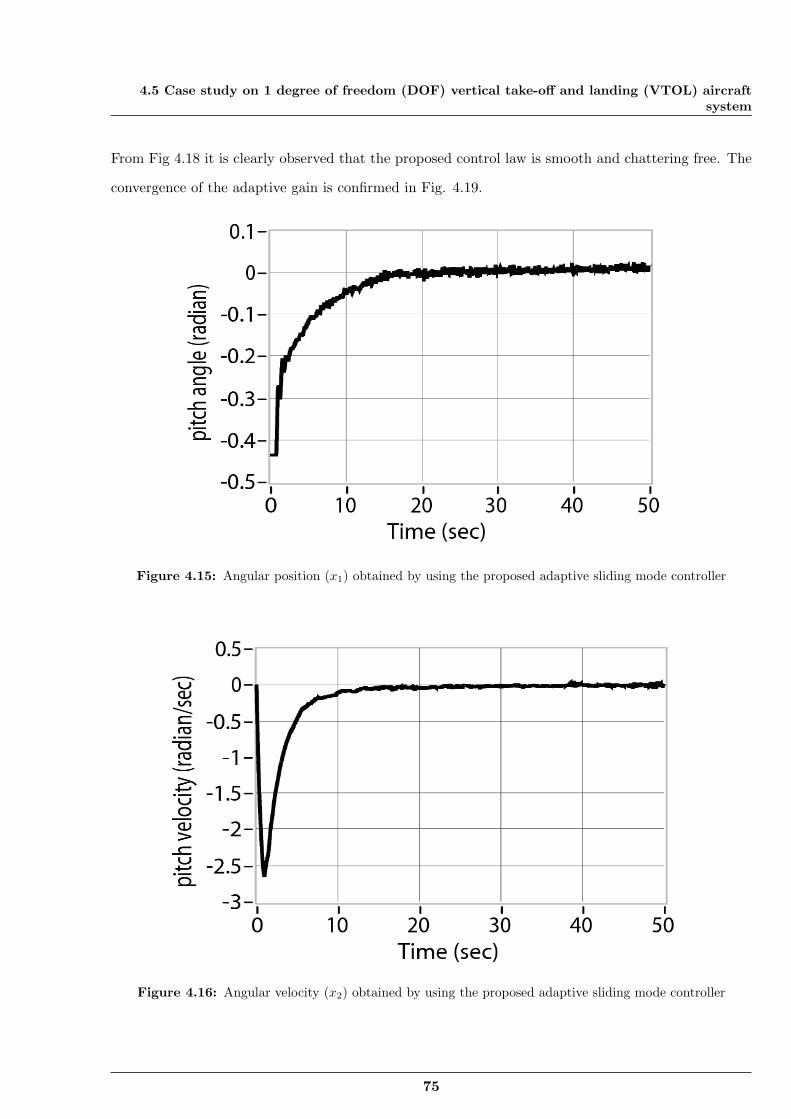
4.5 Case study on 1 degree of freedom (DOF) vertical take-off and landing (VTOL) aircraftsystem
From Fig 4.18 it is clearly observed that the proposed control law is smooth and chattering free. The
convergence of the adaptive gain is confirmed in Fig. 4.19.
Figure 4.15: Angular position (x1) obtained by using the proposed adaptive sliding mode controller
Figure 4.16: Angular velocity (x2) obtained by using the proposed adaptive sliding mode controller
75
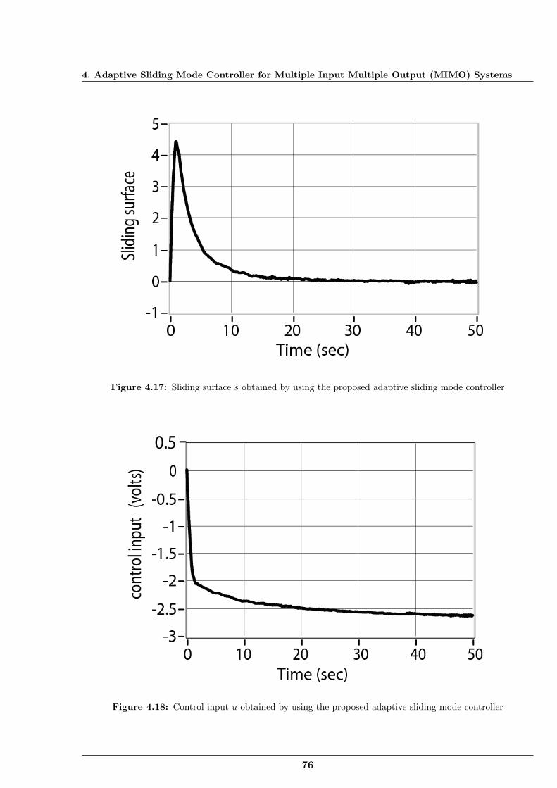
4. Adaptive Sliding Mode Controller for Multiple Input Multiple Output (MIMO) Systems
Figure 4.17: Sliding surface s obtained by using the proposed adaptive sliding mode controller
Figure 4.18: Control input u obtained by using the proposed adaptive sliding mode controller
76
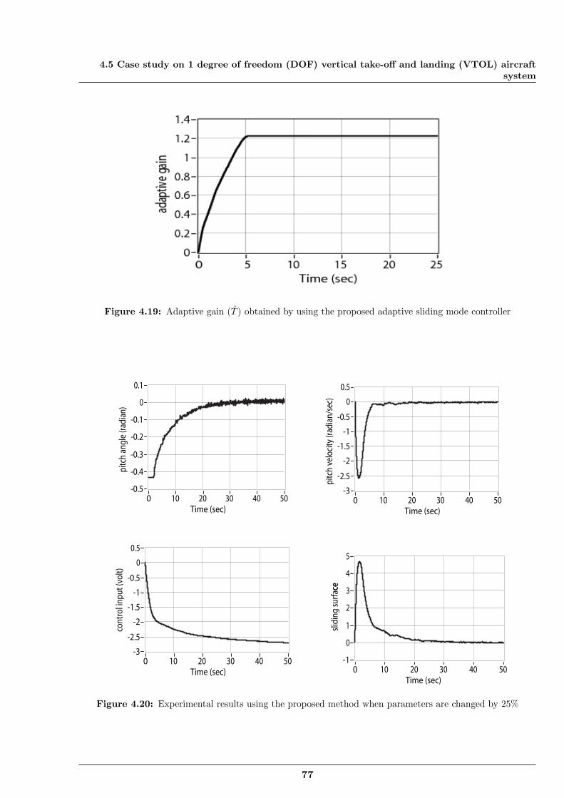
4.5 Case study on 1 degree of freedom (DOF) vertical take-off and landing (VTOL) aircraftsystem
Figure 4.19: Adaptive gain (T ) obtained by using the proposed adaptive sliding mode controller
slid
ing
sur
face
ce
5
-1
0
1
2
3
4
Time (sec) 500 10 20 30 40
con
trol
inp
ut (v
olt)
0.5
-3
-2.5
-2
-1.5
-1
-0.5
0
Time (sec) 500 10 20 30 40
pit
ch a
ngle
(rad
ian)
0.1
-0.5
-0.4
-0.3
-0.2
-0.1
0
Time (sec) 500 10 20 30 40
pit
ch v
eloc
ity
(rad
ian
/sec
)
0.5
-3
-2.5
-2
-1.5
-1
-0.5
0
Time (sec) 500 10 20 30 40
Figure 4.20: Experimental results using the proposed method when parameters are changed by 25%
77
4. Adaptive Sliding Mode Controller for Multiple Input Multiple Output (MIMO) Systems
In order to check the robustness of the proposed adaptive sliding mode controller, the plant param-
eter matrices are perturbed by 25%. In Fig. 4.20, the experimental results are shown with A = 1.25A
and B = 1.25B. It is observed from Fig. 4.20 that the proposed adaptive sliding mode controller
integrated with LESO observer still works reliably demonstrating the robustness of the proposed con-
troller - observer pair.
4.6 Summary
This chapter proposes an adaptive sliding mode (SM) controller for multi-input multi-output
(MIMO) systems. The proposed controller is applied to the twin rotor MIMO system (TRMS) which
is an example of a highly coupled nonlinear system perturbed by mismatched uncertainty. The cross-
coupling between the main and the tail rotor of the TRMS is considered as an uncertainty. An
adaptive tuning rule is designed to deal with the unknown but bounded uncertainty. However, the
upper bound of the system uncertainty is not required to be known apriori as is the case with most
sliding mode controllers. A proportional plus integral sliding surface is used to eliminate the offset
present in the pitch angle. Simulation results show that the proposed adaptive sliding mode controller
demonstrates satisfactory tracking performance and is robust to cross-coupling effect and external
disturbances. Moreover, the proposed adaptive sliding mode controller shows, in general, lesser error
with lower control effort than the PID controllers [84] reported in the literature for the TRMS.
Next, the proposed controller is applied for stabilizing a vertical take-off and landing (VTOL) aircraft
system affected by both matched and mismatched kind of uncertainties. The proposed sliding mode
controller uses a proportional plus integral sliding surface and an adaptive gain tuning law. Prior
knowledge about the upper bound of the system uncertainty, which is the design prerequisite of most
sliding mode controllers, is eliminated by using this adaptive method. Moreover, the adaptive gain
tuning mechanism also ensures that the gain is not overestimated with respect to the actual unknown
value of the uncertainty. Simulation is performed by applying the adaptive sliding mode controller to
the linearized model of the VTOL aircraft. From simulation results, the proposed controller is found
to be superior in chattering mitigation than some already existing similar kind of adaptive sliding
mode controller. Also, the states show faster convergence in the case of the proposed adaptive sliding
mode controller. For application to uncertain systems affected by severe matched and mismatched
78
4.6 Summary
uncertainties like the VTOL aircraft, the proposed adaptive sliding mode control strategy promises
to be a suitable method. Real time experiments conducted on a 1 DOF VTOL system using its
laboratory prototype QNET VTOL are described. The proposed adaptive sliding mode controller
is applied to the 1 DOF VTOL system for tracking a desired reference trajectory and experimental
performance is studied. In the experimental set-up, pitch velocity of the VTOL is the unavailable
state which is required for designing the controller. So a linear extended state observer (LESO) is
combined with the adaptive sliding mode controller to estimate pitch velocity. Experimental results
obtained confirm that the proposed controller is successful in achieving faithful trajectory tracking
for the 1 DOF VTOL. Moreover, chattering in the control input is found to be reduced substantially
corroborating the fact observed earlier in theoretical simulation studies.
79
5Adaptive Terminal Sliding Mode
Controller
Contents
5.1 Introduction . . . . . . . . . . . . . . . . . . . . . . . . . . . . . . . . . . . . 81
5.2 Design of chattering free adaptive terminal sliding mode controller . . . 82
5.3 Stabilization of a triple integrator system . . . . . . . . . . . . . . . . . . 87
5.4 Tracking control of a robotic manipulator . . . . . . . . . . . . . . . . . . . 90
5.5 Summary . . . . . . . . . . . . . . . . . . . . . . . . . . . . . . . . . . . . . . 101
80
5.1 Introduction
5.1 Introduction
It is well recognized that, conventional switching manifolds are usually linear hyper planes which
guarantee asymptotic stability. However, for nonlinear systems, nonlinear sliding surface can also be
selected [12]. In linear sliding mode (LSM), error dynamics cannot converge to zero in finite time
although the parameters can be adjusted to make the convergence arbitrarily fast. However, this
will, in turn, increase the control gain, which may cause severe chattering on the sliding surface and,
therefore, deteriorate the system performance. To tackle the problems of globally asymptotic stabi-
lization, terminal sliding mode (TSM) control scheme has been developed [5, 93–97] to achieve finite
time stabilization. Unfortunately, the terminal sliding mode control features the same drawback of
chattering [30] as in the case of conventional sliding mode control. In [98] a second order sliding mode
controller was developed for multivariable linear systems using the nonsingular terminal sliding man-
ifold. The major disadvantage of this method is that the application is restricted to linear uncertain
systems only and the upper bound of the system uncertainty must be known in advance. In [5, 94]
a continuous finite time control scheme for rigid robotic manipulators affected by uncertainty and
external disturbance was proposed using a new form of terminal sliding mode. In both these methods,
the bound of the uncertainty must be known in advance. Moreover, in these methods a boundary layer
technique is used to replace the discontinuous control action by a saturating continuous approximation
to reduce the chattering. However, its consequence is that invariance property of the SMC is lost.
In this chapter, a chattering free adaptive terminal sliding mode (TSM) controller is proposed to
achieve fast and finite time convergence. In the proposed controller, a nonsingular terminal sliding
manifold is used to design the control law. The time derivative of the control signal is used as the
control input instead of the actual control. The derivative control law is a discontinuous signal because
of the presence of the sign function. However, its integral which is the actual control, is continuous
and hence the chattering is eliminated. An adaptive tuning law is used here to estimate the unknown
uncertainties. This adaptive tuning method does not require prior knowledge about the upper bound
of the system uncertainty for designing the terminal sliding mode controller as was the case with the
terminal sliding mode controllers developed so far [5, 64,93,94,97–99].
The outline of this chapter is as follows. In Section 5.2, the proposed chattering free adaptive terminal
sliding mode (TSM) control strategy is derived. In Section 5.3 the proposed adaptive TSM controller
is applied to stabilize a triple integrator system and the performance is studied. Trajectory tracking
81
5. Adaptive Terminal Sliding Mode Controller
problem of a robotic manipulator is considered in Section 5.4 to investigate the efficacy of the proposed
adaptive TSM controller. Summary is drawn in Section 5.5.
5.2 Design of chattering free adaptive terminal sliding mode con-troller
Let us consider a class of nonlinear system
x = f(x) + ∆f(x) + d(t) +Bu (5.1)
where x = [x1 x2 x3....xn]T ∈ Rn is the state vector. Furthermore, ∆f(x) ∈ Rn is an uncertain term
representing the unmodelled dynamics or structural variation of the system (5.1) and d(t) ∈ Rn is an
external disturbance. Moreover, u ∈ Rm is the input and B is a known matrix of order n ×m. The
uncertainties of the system (5.1) are assumed to be bounded and matched such that ∆f(x) and d(t)
∈ span B. The control objective is to track a given reference signal xd in finite time from any initial
state.
Let the desired state vector be xd = [x1d x2d x3d....xnd]T . The tracking error is defined as,
e = x− xd = [(x1 − x1d) (x2 − x2d) .....(xn − xnd)]T
= [e1, e2, ......en]T . (5.2)
The goal is to design a chattering free adaptive terminal sliding mode controller for a given target xd
such that the resulting tracking error satisfies
limt→∞
||e|| = limt→∞
||x− xd|| → 0 (5.3)
where || · || denotes the Euclidean norm of a vector.
The controller is designed in two steps. At first, a linear sliding surface is defined and then using
the sliding surface, a terminal sliding manifold is obtained so that the derivative of the control input
occurs at the first derivative of the terminal sliding manifold. The actual control input is obtained
by integrating the derivative of the control signal which contains the discontinuous function and thus
eliminates the chattering [27,65,66]. The uncertainty is estimated by using an adaptive tuning law.
A set of sliding surfaces is defined in the error space passing through the origin to represent a sliding
82
5.2 Design of chattering free adaptive terminal sliding mode controller
manifold as fo1lows:
s = [s1, s2, ..., sm]T = cT e = [c1 c2 ...ci...cm]T e
=
c1nen + c1(n−1)en−1 + ...+ c11e1
c2nen + c2(n−1)en−1 + ...+ c21e1
.
cinen + ci(n−1)en−1 + ...+ ci1e1
.
cmnen + cm(n−1)en−1 + ...+ cm1e1
(5.4)
and ci = [cin ci(n−1)....ci1] be such that all roots of the polynomial
ϕ(λ(ei)) = cinλn−1 + ci(n−1)λ
n−2 + ...+ ci1λ (5.5)
are in the open left half-plane [100], i = 1, 2, ..,m. The choice of c determines the convergence rate to
the sliding surface. Let us consider (5.4), where e = x− xd. The first time derivative of (5.4) yields
s = cT e
= cT (x− xd) (5.6)
Using (5.1) and (5.6) yields,
s = cT (f(x) + ∆f(x) + d(t) +Bu− xd) (5.7)
Taking the derivative of (5.7) gives rise to
s = cT (d
dtf(x) +
d
dt∆f(x) + d(t) +Bu− xd)
= cT (f(x) + ∆f(x) + d(t) +Bu− xd) (5.8)
A nonsingular terminal sliding mode manifold is first designed as
σ = s+ βspq (5.9)
Here β = diag(β1, β2, ...., βn) is a positive constant and p/q (p and q are positive odd integers) is chosen
in such a way that the condition 1 < pq < 2 holds [94]. The linear sliding surface s is combined with
the nonsingular terminal sliding manifold σ to realize the terminal sliding mode control. As σ reaches
83
5. Adaptive Terminal Sliding Mode Controller
zero in finite time, both s and s are bound to reach zero. Then, the tracking error e asymptotically
converges to zero.
Taking the time derivative of (5.9) yields,
σ = s+ β(p
q)s
pq−1s
= β(p
q)s
pq−1(s+ β−1(
p
q)−1s
2−( pq)) (5.10)
Assumption 5.1. The first time derivative of the uncertain term, ∆f(x) and the first time derivative
of the disturbance, d(t) are assumed to be bounded and satisfy the following condition:
||cT (∆f(x) + d(t))|| ≤r∑i=0
Bi||x||i r = 0, 1, ..n (5.11)
where Bi are unknown positive constants, which are not easily obtained due to the complicated structure
of the uncertainties in practical control systems. The number of adaptive rules r is determined by the
designer in accordance with the knowledge of the relative order of perturbation that the system might
encounter. For designing the traditional sliding mode controller, one usually assumes that the upper
bound of lumped perturbations satisfies certain conditions. For example, if r = 0, then the nature of
the disturbance is periodic and it is well represented by a known constant value. If we choose r = 1,
it covers more area in the range space rather than when r = 0 is considered. Thus rest of the control
law is designed by considering r = 1.
It will be proven in Theorem 5.1 that since the derivative of the control input contains the discon-
tinuous term, the actual control signal which will be obtained after the integration operation will not
contain any high frequency switching component. Thus the proposed terminal sliding mode controller
will be free from the chattering phenomenon. Moreover, the controller does not need prior knowledge
about the upper bound of the disturbance. Instead, the upper bound is obtained by designing an
adaptive tuning law.
Theorem 5.1. Considering the uncertain system (5.1), the tracking error dynamics (5.6) can asymp-
totically converge to zero if the nonsingular terminal sliding manifold is chosen as (5.9) and the control
law is obtained as follows:
u = −(cTB)−1[cT f(x) + β−1(p
q)−1s
2−( pq) + (B0 + B1||x||)sign(σ) +K†σ − cT xd] (5.12)
84
5.2 Design of chattering free adaptive terminal sliding mode controller
where (cTB)−1 is nonsingular, B0 , B1 and K† = diag(K†1....K
†m) > 0 are the designed parameters.
In practice the bounds of the uncertain term (B0 + B1||x||) in (5.12) is often difficult to know. Hence
an adaptive tuning law is designed to determine B0 and B1. So the control law is represented as,
u = −(cTB)−1
∫ t
0[cT f(x)dτ + β−1(
p
q)−1s
2−( pq) + ( ˆB0 + ˆB1||x||)sign(σ) +K†σ − cT xd]dτ(5.13)
where ˆB0 and ˆB1 estimate the bounds of uncertainty, i.e. cT (||∆f(x)+ d(t)||) ≤ B0 + B1||x||. Defining
the adaptation error as ˜B0 = ˆB0−B0 and ˜B1 = ˆB1−B1, the parameter ˆB0 and ˆB1 are to be estimated
by using the adaptation law
˙B0 =
1ν0
(p
q)||β|| ||s(
pq)−1
σ|| (5.14)
and
˙B1 =
1ν1
(p
q)||β|| ||s(
pq)−1
σ|| ||x|| (5.15)
where ν0 and ν1 are the positive tuning parameters.
Proof : Let us consider the following Lyapunov function
V (t) =12σTσ +
12ν0
˜B20 +
12ν1
˜B21 (5.16)
Using (5.8 - 5.15), the time derivative of the Lyapunov function V (t) is obtained as,
V (t) = σT σ + ν0˜B0
˙B0 + ν1
˜B1˙B1
= β(p
q)s(
pq)−1
σT (s+ β−1(p
q)−1s
2−( pq)) + ν0( ˆB0 − B0)
˙B0 + ν1( ˆB1 − B1)
˙B1
= β(p
q)s(
pq)−1
σT [cT (d
dtf(x) +
d
dt∆f(x) + d(t) +Bu− xd) + β−1(
p
q)−1s
2−( pq)]
+( ˆB0 − B0)(p
q)||β|| ||s(
pq)−1
σ|| + ( ˆB1 − B1)(p
q)||β|| ||s(
pq)−1
σ|| ||x||
≤ ||β||(pq)||s(
pq)−1
σT || [B0 + B1||x|| −K†||σ|| − ( ˆB0 + ˆB1||x||)sign(σ)]
+( ˆB0 − B0)(p
q)||β|| ||s(
pq)−1
σ|| + ( ˆB1 − B1)(p
q)||β|| ||s(
pq)−1
σ|| ||x||
≤ −K†||σ|| (5.17)
The above inequality holds if˙B0 = 1
ν0(pq )||β|| ||s
( pq)−1
σ|| and˙B1 = 1
ν1(pq )||β|| ||s
( pq)−1
σ|| ||x||. Moreover,
||s(pq)−1|| > 0 for any s = 0 and s(
pq)−1 = 0 only when s = 0. Therefore, the convergence to a domain
σ = 0 is guaranteed from any initial condition [30].
85
5. Adaptive Terminal Sliding Mode Controller
Suppose that tr is the time when σ reaches zero from σ(0) = 0 , i.e. σ = 0 for all t ≥ tr. Once σ
reaches zero, it will stay at zero using the control law (5.12). Thus the sliding surface s will converge
to zero in finite time tf . The total time from σ(0) = 0 to stf can be calculated by using the equation
s+ βs( p
q) = 0 (5.9) from which the time taken from str to stf [94] is obtained as,
tf = tr +(pq )
(pq ) − 1β−( p
q)||str||(
pq)−1 (5.18)
Hence the error (5.2) asymptotically converges to zero and the system reaches the equilibrium. This
completes the proof.
Remark 5.1. Practically, ||σ|| cannot become exactly zero in finite time and thus the adaptive pa-
rameter˙Bi may increase boundlessly. A simple way of overcoming this disadvantage is to use the dead
zone technique [30] and modify the adaptive tuning law (5.14 - 5.15) as,
˙B0 =
1ν0
(pq )||β|| ||s( p
q)−1
σ||, ||σ|| ≥ ε
0, ||σ|| < ε(5.19)
and
˙B1 =
1ν1
(pq )||β|| s( p
q)−1
σ|| ||x||, ||σ|| ≥ ε
0, ||σ|| < ε(5.20)
where ε is a small positive constant.
Remark 5.2. The parameter ϵ in controller (5.13) is very important and it is one of the parameters
determining the convergence rate of the sliding surface. It is clear that a large ϵ will force the system
states to converge to the origin with a high speed. However, a very large value of ϵ will require a very
high control input but in reality it is always bounded. Thus the parameter ϵ cannot be selected to be
too large. In practice, a compromise has to be made between the response speed and the control input.
Remark 5.3.The parameters ν0 and ν1 in (5.14 - 5.15) determine the convergence rate of the esti-
mated bounds ˆB0 and ˆB1. Large values of ν0 and ν1 can be chosen to force the estimated bounds ˆB0
and ˆB1 to rapidly converge to the actual bounds.
Remark 5.4. An exact robust differentiator is available for accurately measuring or estimating the
derivative of variables.
86
5.3 Stabilization of a triple integrator system
5.3 Stabilization of a triple integrator system
The adaptive terminal sliding mode controller proposed above is applied to a triple integrator
system with uncertainty as described below [62],
x1 = x2
x2 = x3
x3 = u+ p(x)y = x1 (5.21)
where p(x) = 7sin(10x1) is the bounded uncertainty, y is the output and the initial condition of
the system is assumed as x(0) = [1 0 − 1]T [61]. The desired state is xd = [0 0 0]T as it is a
stabilization problem. Hence in this case the error and state are equivalent i.e, e = x− xd = x.
The third order sliding mode controller presented by Defoort et al. [4] using twisting sliding modes
to achieve finite time control is compared with the proposed adaptive TSM controller. As explained
in [61] and [62], the control for the system given by (5.21) can be obtained as [4],
u = unom + udisk (5.22)
Let k1, k2, ..., kn > 0 be such that the polynomial λn + knλn−1 + ...+ k2λ+ k1 is Hurwitz. The system
(5.21) can be stabilized to the origin using the feedback control law given in [4, 61,62] as
unom = −k1sign(x1)|x1|α1 − k2sign(x2)|x2|α2 ...− knsign(xn)|xn|αn (5.23)
where α1, ..., αn satisfy αi−1 =αiαi+1
2αi+1 − αifor i = 2, ..., n with αn+1 = 1 (5.24)
With n = 3, k1 = 1, k2 = k3 = 1.5 and α3 = 3/4, the control law (5.22) can be expressed as [4],
unom = −sign(x1)|x1|12 − 1.5sign(x2)|x2|
35 − 1.5sign(x3)|x3|
34
udisk = udisk,1 + udisk,2 (5.25)
where the sliding surface σ = x3 −∫ t0 unomdτ and udisk is given by [4],
udisk,1 = −ζ∫ t
0sign(σ)τ
udisk,2 = −ϑ|σ|12 sign(σ) (5.26)
87
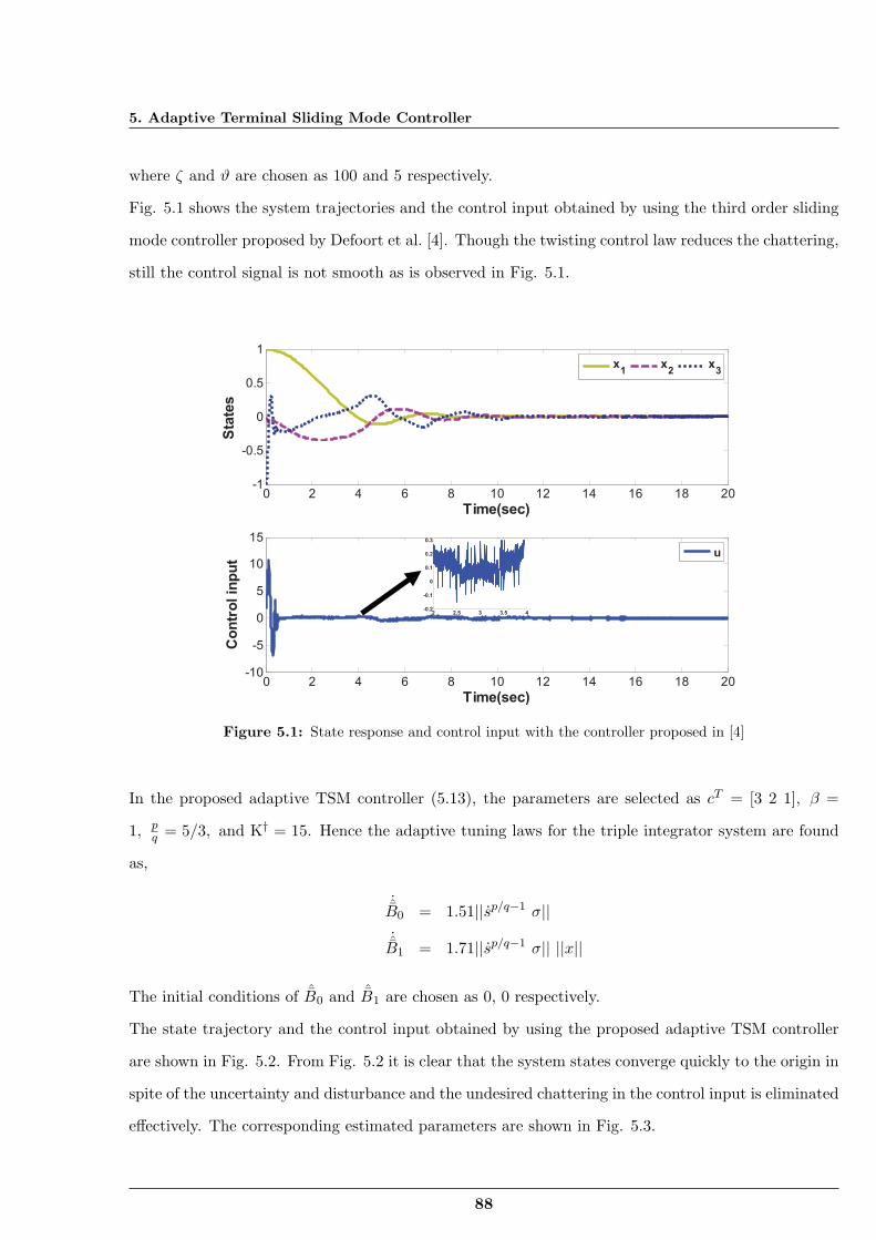
5. Adaptive Terminal Sliding Mode Controller
where ζ and ϑ are chosen as 100 and 5 respectively.
Fig. 5.1 shows the system trajectories and the control input obtained by using the third order sliding
mode controller proposed by Defoort et al. [4]. Though the twisting control law reduces the chattering,
still the control signal is not smooth as is observed in Fig. 5.1.
0 2 4 6 8 10 12 14 16 18 20-1
-0.5
0
0.5
1
Time(sec)
Sta
tes
x1
x2
x3
0 2 4 6 8 10 12 14 16 18 20-10
-5
0
5
10
15
Time(sec)
Co
ntr
ol in
pu
t
u
2 2.5 3 3.5 4-0.2
-0.1
0
0.1
0.2
0.3
Figure 5.1: State response and control input with the controller proposed in [4]
In the proposed adaptive TSM controller (5.13), the parameters are selected as cT = [3 2 1], β =
1, pq = 5/3, and K† = 15. Hence the adaptive tuning laws for the triple integrator system are found
as,
˙B0 = 1.51||sp/q−1 σ||˙B1 = 1.71||sp/q−1 σ|| ||x||
The initial conditions of ˆB0 and ˆB1 are chosen as 0, 0 respectively.
The state trajectory and the control input obtained by using the proposed adaptive TSM controller
are shown in Fig. 5.2. From Fig. 5.2 it is clear that the system states converge quickly to the origin in
spite of the uncertainty and disturbance and the undesired chattering in the control input is eliminated
effectively. The corresponding estimated parameters are shown in Fig. 5.3.
88
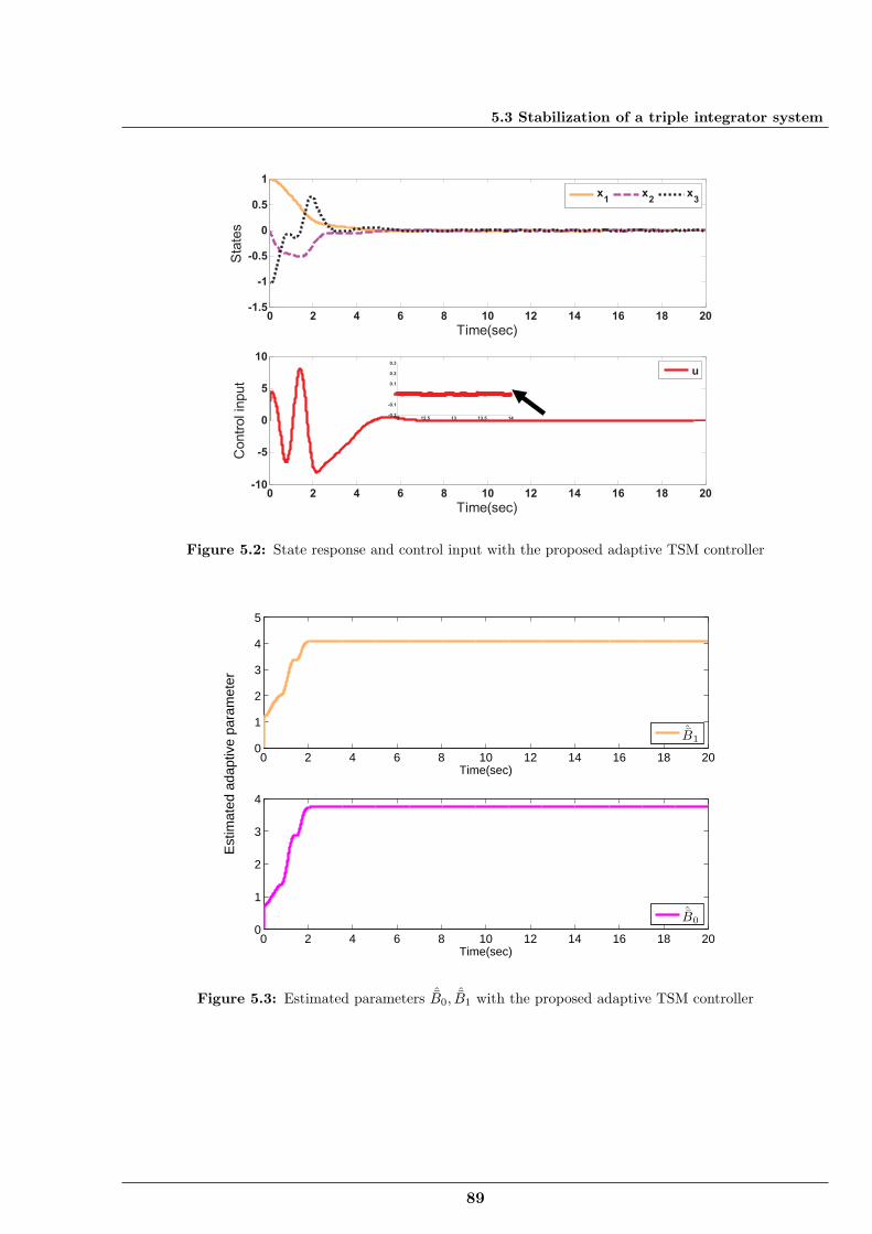
5.3 Stabilization of a triple integrator system
0 2 4 6 8 10 12 14 16 18 20-1.5
-1
-0.5
0
0.5
1
Time(sec)
Sta
tes
x1
x2
x3
0 2 4 6 8 10 12 14 16 18 20-10
-5
0
5
10
Time(sec)
Contr
ol in
put
u
12 12.5 13 13.5 14-0.2
-0.1
0
0.1
0.2
0.3
Figure 5.2: State response and control input with the proposed adaptive TSM controller
0 2 4 6 8 10 12 14 16 18 200
1
2
3
4
5
Time(sec)
ˆB1
0 2 4 6 8 10 12 14 16 18 200
1
2
3
4
Time(sec)
Est
imat
ed a
dapt
ive
para
met
er
ˆB0
Figure 5.3: Estimated parameters ˆB0,ˆB1 with the proposed adaptive TSM controller
89
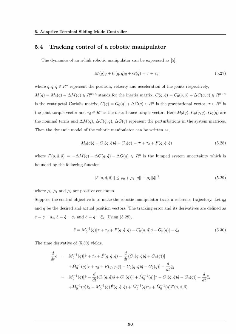
5. Adaptive Terminal Sliding Mode Controller
5.4 Tracking control of a robotic manipulator
The dynamics of an n-link robotic manipulator can be expressed as [5],
M(q)q + C(q, q)q +G(q) = τ + τd (5.27)
where q, q, q ∈ Rn represent the position, velocity and acceleration of the joints respectively,
M(q) = M0(q) + ∆M(q) ∈ Rn×n stands for the inertia matrix, C(q, q) = C0(q, q) + ∆C(q, q) ∈ Rn×n
is the centripetal Coriolis matrix, G(q) = G0(q) + ∆G(q) ∈ Rn is the gravitational vector, τ ∈ Rn is
the joint torque vector and τd ∈ Rn is the disturbance torque vector. Here M0(q), C0(q, q), G0(q) are
the nominal terms and ∆M(q), ∆C(q, q), ∆G(q) represent the perturbations in the system matrices.
Then the dynamic model of the robotic manipulator can be written as,
M0(q)q + C0(q, q)q +G0(q) = τ + τd + F (q, q, q) (5.28)
where F (q, q, q) = −∆M(q) − ∆C(q, q) − ∆G(q) ∈ Rn is the lumped system uncertainty which is
bounded by the following function
||F (q, q, q)|| ≤ ρ0 + ρ1||q|| + ρ2||q||2 (5.29)
where ρ0, ρ1 and ρ2 are positive constants.
Suppose the control objective is to make the robotic manipulator track a reference trajectory. Let qd
and q be the desired and actual position vectors. The tracking error and its derivatives are defined as
e = q − qd, e = q − qd and e = q − qd. Using (5.28),
e = M−10 (q)[τ + τd + F (q, q, q) − C0(q, q)q −G0(q)] − qd (5.30)
The time derivative of (5.30) yields,
d
dte = M−1
0 (q)[τ + τd + F (q, q, q) − d
dt(C0(q, q)q +G0(q))]
+M−10 (q)[τ + τd + F (q, q, q) − C0(q, q)q −G0(q)] −
d
dtqd
= M−10 (q)[τ − d
dt(C0(q, q)q +G0(q))] + M−1
0 (q)[τ − C0(q, q)q −G0(q)] −d
dtqd
+M−10 (q)τd +M−1
0 (q)F (q, q, q) + M−10 (q)τd + M−1
0 (q)F (q, q, q)
90
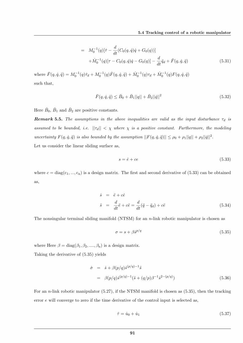
5.4 Tracking control of a robotic manipulator
= M−10 (q)[τ − d
dt(C0(q, q)q +G0(q))]
+M−10 (q)[τ − C0(q, q)q −G0(q)] −
d
dtqd + F (q, q, q) (5.31)
where F (q, q, q) = M−10 (q)τd +M−1
0 (q)F (q, q, q) + M−10 (q)τd + M−1
0 (q)F (q, q, q)
such that,
F (q, q, q) ≤ B0 + B1||q|| + B2||q||2 (5.32)
Here B0, B1 and B2 are positive constants.
Remark 5.5. The assumptions in the above inequalities are valid as the input disturbance τd is
assumed to be bounded, i.e. ||τd|| < χ where χ is a positive constant. Furthermore, the modeling
uncertainty F (q, q, q) is also bounded by the assumption ||F (q, q, q)|| ≤ ρ0 + ρ1||q|| + ρ2||q||2.
Let us consider the linear sliding surface as,
s = e+ ce (5.33)
where c = diag(c1, ..., cn) is a design matrix. The first and second derivative of (5.33) can be obtained
as,
s = e+ ce
s =d
dte+ ce =
d
dt(q − qd) + ce (5.34)
The nonsingular terminal sliding manifold (NTSM) for an n-link robotic manipulator is chosen as
σ = s+ βsp/q (5.35)
where Here β = diag(β1, β2, ...., βn) is a design matrix.
Taking the derivative of (5.35) yields
σ = s+ β(p/q)s(p/q)−1s
= β(p/q)s(p/q)−1(s+ (q/p)β−1s2−(p/q)) (5.36)
For an n-link robotic manipulator (5.27), if the NTSM manifold is chosen as (5.35), then the tracking
error e will converge to zero if the time derivative of the control input is selected as,
τ = u0 + u1 (5.37)
91
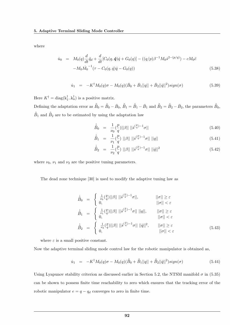
5. Adaptive Terminal Sliding Mode Controller
where
u0 = M0(q)d
dtqd +
d
dt[C0(q, q)q +G0(q)] − ((q/p)β−1M0s
2−(p/q)) − cM0e
−M0M0−1
(τ − C0(q, q)q −G0(q)) (5.38)
u1 = −K†M0(q)σ −M0(q)(B0 + B1||q|| + B2||q||2)sign(σ) (5.39)
Here K† = diag(k†1..k†n) is a positive matrix.
Defining the adaptation error as ˜B0 = ˆB0 − B0, ˜B1 = ˆB1 − B1 and ˜B2 = ˆB2 − B2, the parameters ˆB0,
ˆB1 and ˆB2 are to be estimated by using the adaptation law
˙B0 =
1ν0
(p
q)||β|| ||s(
pq)−1
σ|| (5.40)
˙B1 =
1ν1
(p
q) ||β|| ||s(
pq)−1
σ|| ||q|| (5.41)
˙B2 =
1ν2
(p
q) ||β|| ||s(
pq)−1
σ|| ||q||2 (5.42)
where ν0, ν1 and ν2 are the positive tuning parameters.
The dead zone technique [30] is used to modify the adaptive tuning law as
˙B0 =
1ν0
(pq )||β|| ||s( p
q)−1
σ||, ||σ|| ≥ ε
0, ||σ|| < ε
˙B1 =
1ν1
(pq )||β|| ||s( p
q)−1
σ|| ||q||, ||σ|| ≥ ε
0, ||σ|| < ε
˙B2 =
1ν2
(pq )||β|| ||s( p
q)−1
σ|| ||q||2, ||σ|| ≥ ε
0, ||σ|| < ε(5.43)
where ε is a small positive constant.
Now the adaptive terminal sliding mode control law for the robotic manipulator is obtained as,
u1 = −K†M0(q)σ −M0(q)( ˆB0 + ˆB1||q|| + ˆB2||q||2)sign(σ) (5.44)
Using Lyapunov stability criterion as discussed earlier in Section 5.2, the NTSM manifold σ in (5.35)
can be shown to possess finite time reachability to zero which ensures that the tracking error of the
robotic manipulator e = q − qd converges to zero in finite time.
92
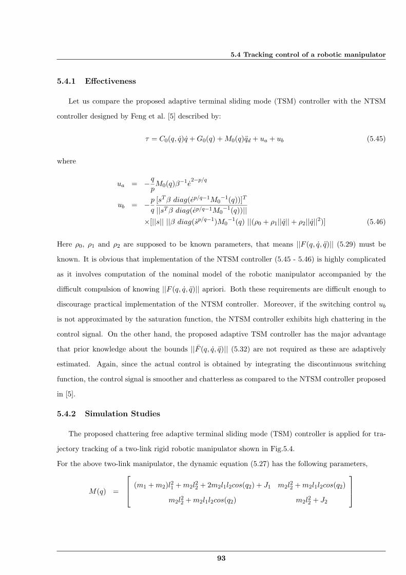
5.4 Tracking control of a robotic manipulator
5.4.1 Effectiveness
Let us compare the proposed adaptive terminal sliding mode (TSM) controller with the NTSM
controller designed by Feng et al. [5] described by:
τ = C0(q, q)q +G0(q) +M0(q)qd + ua + ub (5.45)
where
ua = −qpM0(q)β−1e
2−p/q
ub = −pq
[sTβ diag(ep/q−1M0−1(q))]T
||sTβ diag(ep/q−1M0−1(q))||
×[||s|| ||β diag(sp/q−1)M0−1(q) ||(ρ0 + ρ1||q|| + ρ2||q||2)] (5.46)
Here ρ0, ρ1 and ρ2 are supposed to be known parameters, that means ||F (q, q, q)|| (5.29) must be
known. It is obvious that implementation of the NTSM controller (5.45 - 5.46) is highly complicated
as it involves computation of the nominal model of the robotic manipulator accompanied by the
difficult compulsion of knowing ||F (q, q, q)|| apriori. Both these requirements are difficult enough to
discourage practical implementation of the NTSM controller. Moreover, if the switching control ub
is not approximated by the saturation function, the NTSM controller exhibits high chattering in the
control signal. On the other hand, the proposed adaptive TSM controller has the major advantage
that prior knowledge about the bounds ||F (q, q, q)|| (5.32) are not required as these are adaptively
estimated. Again, since the actual control is obtained by integrating the discontinuous switching
function, the control signal is smoother and chatterless as compared to the NTSM controller proposed
in [5].
5.4.2 Simulation Studies
The proposed chattering free adaptive terminal sliding mode (TSM) controller is applied for tra-
jectory tracking of a two-link rigid robotic manipulator shown in Fig.5.4.
For the above two-link manipulator, the dynamic equation (5.27) has the following parameters,
M(q) =
(m1 +m2)l21 +m2l22 + 2m2l1l2cos(q2) + J1 m2l
22 +m2l1l2cos(q2)
m2l22 +m2l1l2cos(q2) m2l
22 + J2
93
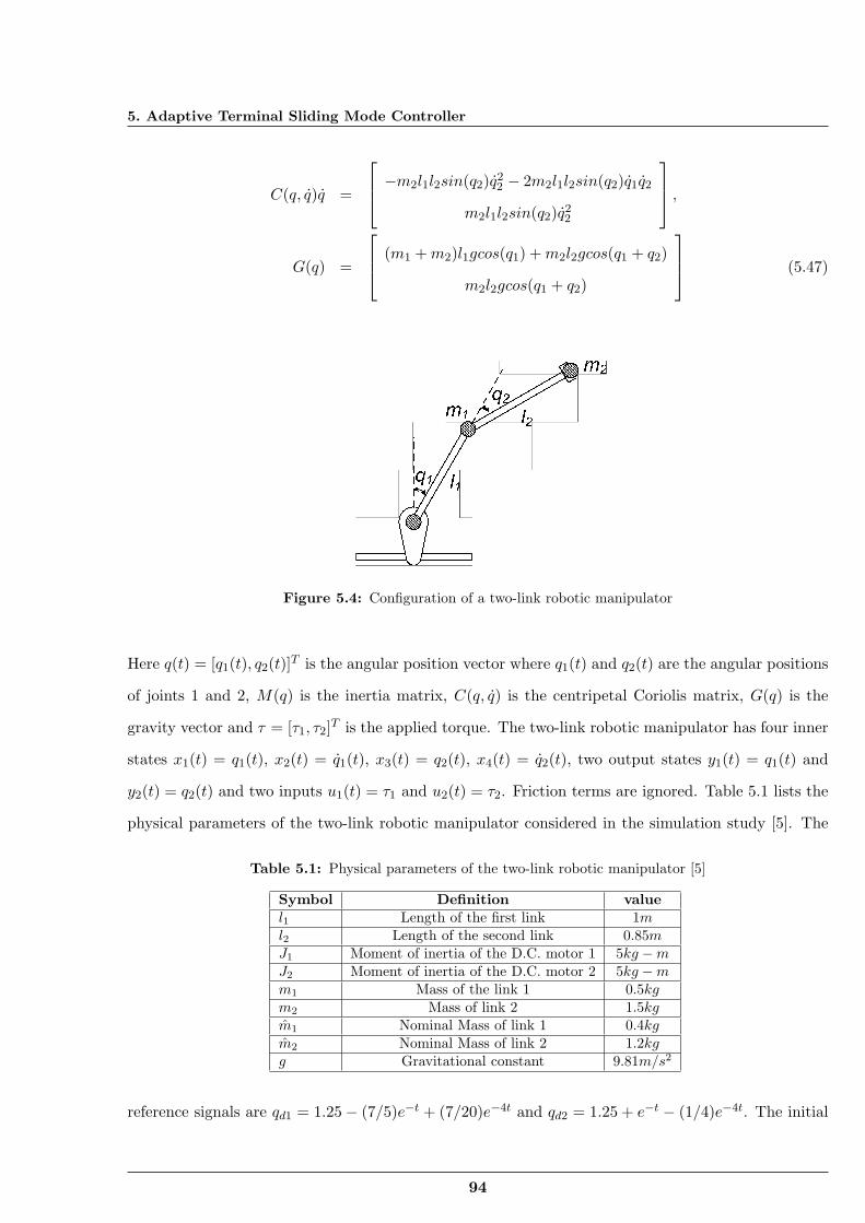
5. Adaptive Terminal Sliding Mode Controller
C(q, q)q =
−m2l1l2sin(q2)q22 − 2m2l1l2sin(q2)q1q2
m2l1l2sin(q2)q22
,G(q) =
(m1 +m2)l1gcos(q1) +m2l2gcos(q1 + q2)
m2l2gcos(q1 + q2)
(5.47)
Figure 5.4: Configuration of a two-link robotic manipulator
Here q(t) = [q1(t), q2(t)]T is the angular position vector where q1(t) and q2(t) are the angular positions
of joints 1 and 2, M(q) is the inertia matrix, C(q, q) is the centripetal Coriolis matrix, G(q) is the
gravity vector and τ = [τ1, τ2]T is the applied torque. The two-link robotic manipulator has four inner
states x1(t) = q1(t), x2(t) = q1(t), x3(t) = q2(t), x4(t) = q2(t), two output states y1(t) = q1(t) and
y2(t) = q2(t) and two inputs u1(t) = τ1 and u2(t) = τ2. Friction terms are ignored. Table 5.1 lists the
physical parameters of the two-link robotic manipulator considered in the simulation study [5]. The
Table 5.1: Physical parameters of the two-link robotic manipulator [5]
Symbol Definition valuel1 Length of the first link 1ml2 Length of the second link 0.85mJ1 Moment of inertia of the D.C. motor 1 5kg −mJ2 Moment of inertia of the D.C. motor 2 5kg −mm1 Mass of the link 1 0.5kgm2 Mass of link 2 1.5kgm1 Nominal Mass of link 1 0.4kgm2 Nominal Mass of link 2 1.2kgg Gravitational constant 9.81m/s2
reference signals are qd1 = 1.25 − (7/5)e−t + (7/20)e−4t and qd2 = 1.25 + e−t − (1/4)e−4t. The initial
94
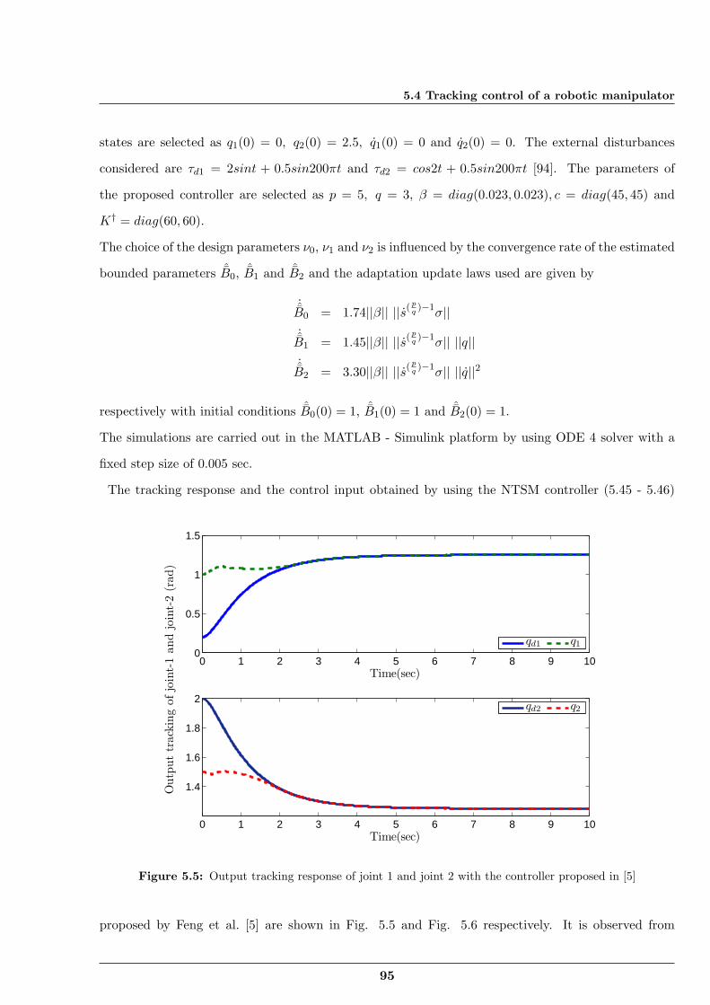
5.4 Tracking control of a robotic manipulator
states are selected as q1(0) = 0, q2(0) = 2.5, q1(0) = 0 and q2(0) = 0. The external disturbances
considered are τd1 = 2sint + 0.5sin200πt and τd2 = cos2t + 0.5sin200πt [94]. The parameters of
the proposed controller are selected as p = 5, q = 3, β = diag(0.023, 0.023), c = diag(45, 45) and
K† = diag(60, 60).
The choice of the design parameters ν0, ν1 and ν2 is influenced by the convergence rate of the estimated
bounded parameters ˆB0, ˆB1 and ˆB2 and the adaptation update laws used are given by
˙B0 = 1.74||β|| ||s(
pq)−1
σ||˙B1 = 1.45||β|| ||s(
pq)−1
σ|| ||q||˙B2 = 3.30||β|| ||s(
pq)−1
σ|| ||q||2
respectively with initial conditions ˆB0(0) = 1, ˆB1(0) = 1 and ˆB2(0) = 1.
The simulations are carried out in the MATLAB - Simulink platform by using ODE 4 solver with a
fixed step size of 0.005 sec.
The tracking response and the control input obtained by using the NTSM controller (5.45 - 5.46)
0 1 2 3 4 5 6 7 8 9 100
0.5
1
1.5
Time(sec)
qd1 q1
0 1 2 3 4 5 6 7 8 9 10
1.4
1.6
1.8
2
Time(sec)
Outp
ut
track
ing
ofjo
int-
1and
join
t-2
(rad)
qd2 q2
Figure 5.5: Output tracking response of joint 1 and joint 2 with the controller proposed in [5]
proposed by Feng et al. [5] are shown in Fig. 5.5 and Fig. 5.6 respectively. It is observed from
95
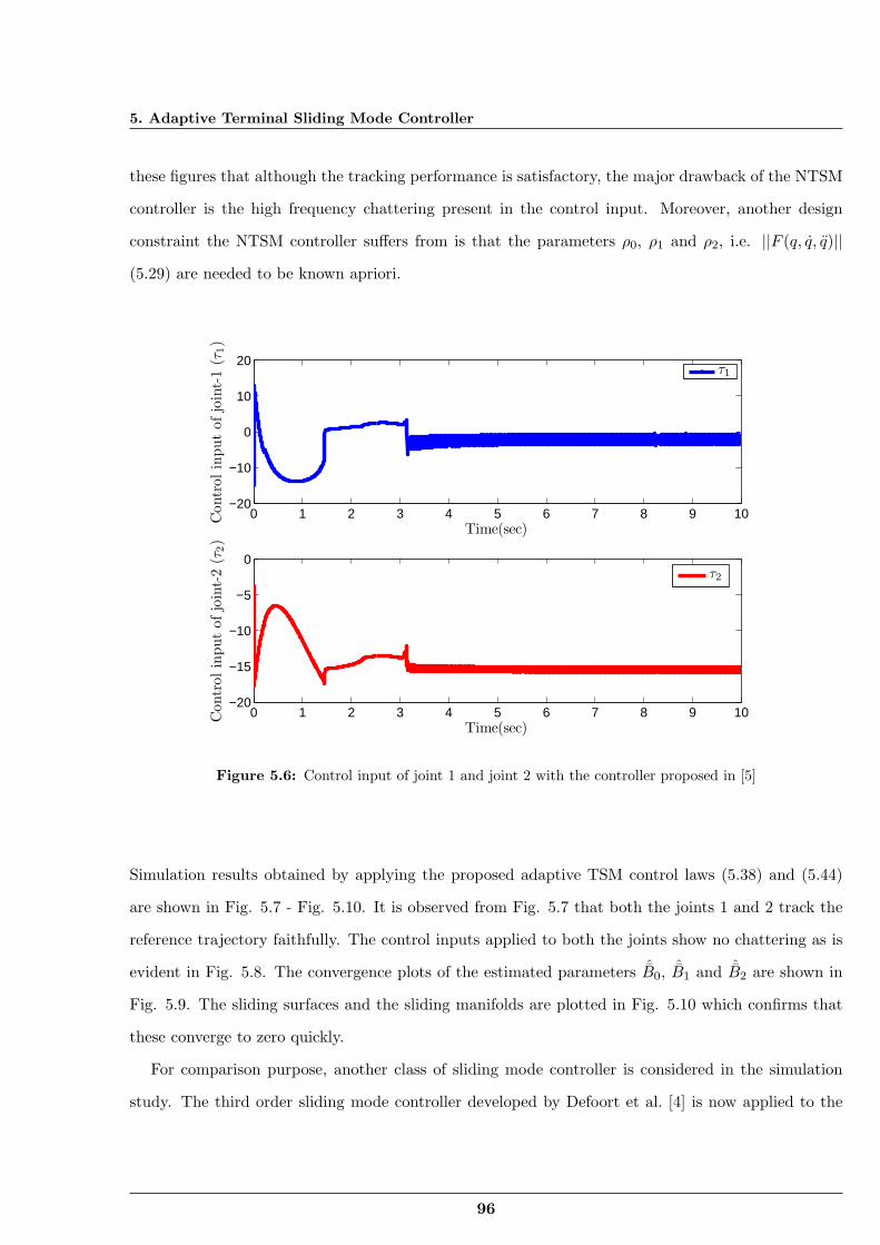
5. Adaptive Terminal Sliding Mode Controller
these figures that although the tracking performance is satisfactory, the major drawback of the NTSM
controller is the high frequency chattering present in the control input. Moreover, another design
constraint the NTSM controller suffers from is that the parameters ρ0, ρ1 and ρ2, i.e. ||F (q, q, q)||
(5.29) are needed to be known apriori.
0 1 2 3 4 5 6 7 8 9 10−20
−10
0
10
20
Time(sec)
Contr
olin
put
ofjo
int-
1(τ
1)
τ1
0 1 2 3 4 5 6 7 8 9 10−20
−15
−10
−5
0
Time(sec)
Contr
olin
put
ofjo
int-
2(τ
2)
τ2
Figure 5.6: Control input of joint 1 and joint 2 with the controller proposed in [5]
Simulation results obtained by applying the proposed adaptive TSM control laws (5.38) and (5.44)
are shown in Fig. 5.7 - Fig. 5.10. It is observed from Fig. 5.7 that both the joints 1 and 2 track the
reference trajectory faithfully. The control inputs applied to both the joints show no chattering as is
evident in Fig. 5.8. The convergence plots of the estimated parameters ˆB0, ˆB1 and ˆB2 are shown in
Fig. 5.9. The sliding surfaces and the sliding manifolds are plotted in Fig. 5.10 which confirms that
these converge to zero quickly.
For comparison purpose, another class of sliding mode controller is considered in the simulation
study. The third order sliding mode controller developed by Defoort et al. [4] is now applied to the
96
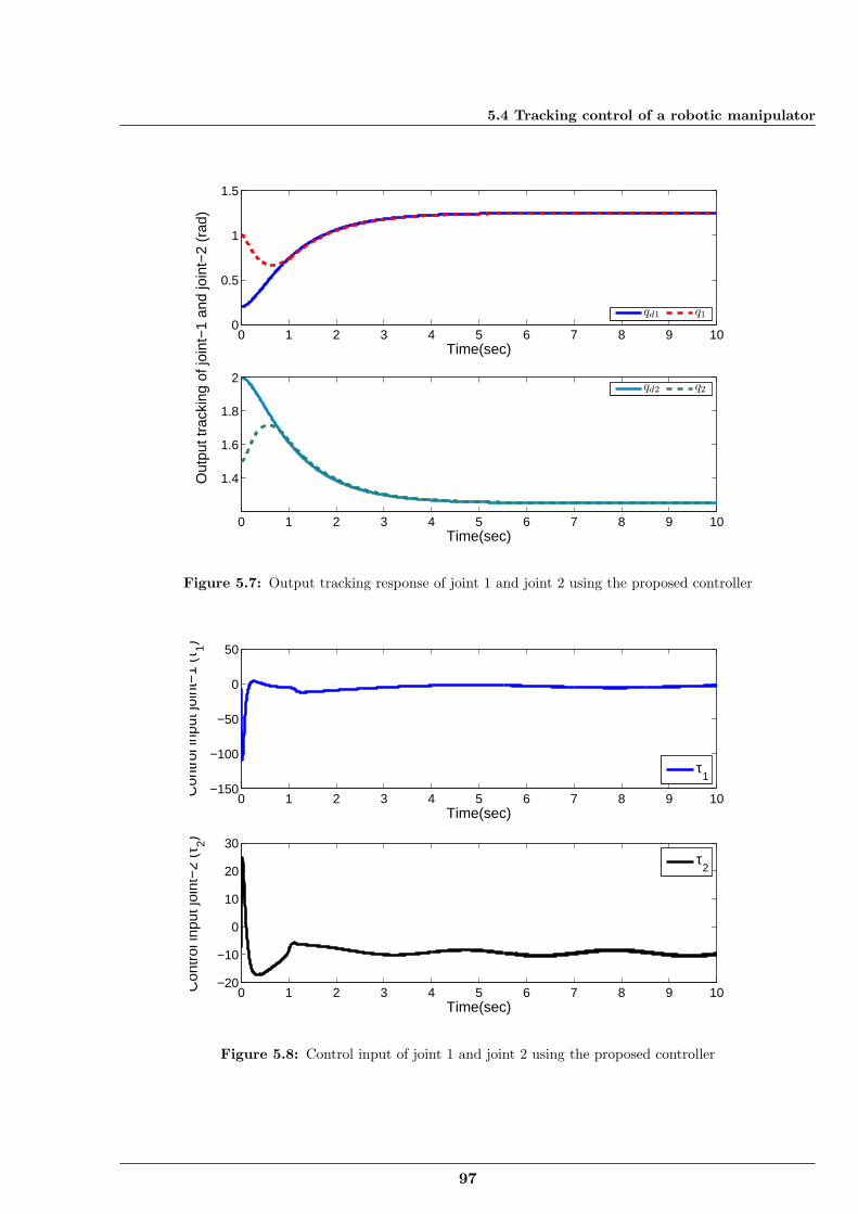
5.4 Tracking control of a robotic manipulator
0 1 2 3 4 5 6 7 8 9 100
0.5
1
1.5
Time(sec)
Out
put t
rack
ing
of jo
int−
1 an
d jo
int−
2 (r
ad)
qd1 q1
0 1 2 3 4 5 6 7 8 9 10
1.4
1.6
1.8
2
Time(sec)
qd2 q2
Figure 5.7: Output tracking response of joint 1 and joint 2 using the proposed controller
0 1 2 3 4 5 6 7 8 9 10−150
−100
−50
0
50
Time(sec)
Con
trol
inpu
t joi
nt−
1 (τ
1)
τ1
0 1 2 3 4 5 6 7 8 9 10−20
−10
0
10
20
30
Time(sec)
Con
trol
inpu
t joi
nt−
2 (τ
2)
τ2
Figure 5.8: Control input of joint 1 and joint 2 using the proposed controller
97
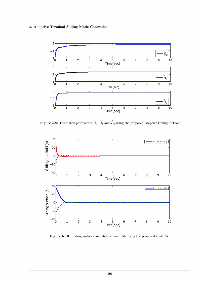
5. Adaptive Terminal Sliding Mode Controller
0 1 2 3 4 5 6 7 8 9 101
1.5
2
Time(sec)
Pra
ram
eter
estim
ation:
B0,B
1and
B2
ˆB0
0 1 2 3 4 5 6 7 8 9 101
2
3
Time(sec)
ˆB1
0 1 2 3 4 5 6 7 8 9 101
1.5
2
Time(sec)
ˆB2
Figure 5.9: Estimated parameters ˆB0, ˆB1 and ˆB2 using the proposed adaptive tuning method
0 1 2 3 4 5 6 7 8 9 10−40
−20
0
20
40
Time(sec)
Slid
ing
man
ifold
(σ)
σ1 σ2
0 1 2 3 4 5 6 7 8 9 10−40
−20
0
20
40
Time(sec)
Slid
ing
surf
ace
(s)
s1 s2
Figure 5.10: Sliding surfaces and sliding manifolds using the proposed controller
98
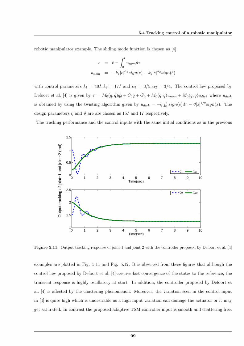
5.4 Tracking control of a robotic manipulator
robotic manipulator example. The sliding mode function is chosen as [4]
s = e−∫ t
0unomdτ
unom = −k1|e|α1sign(e) − k2|e|α2sign(e)
with control parameters k1 = 40I, k2 = 17I and α1 = 3/5, α2 = 3/4. The control law proposed by
Defoort et al. [4] is given by τ = M0(q, q)qd + C0q +G0 +M0(q, q)unom +M0(q, q)udisk where udisk
is obtained by using the twisting algorithm given by udisk = −ζ∫ t0 sign(s)dτ − ϑ|s|1/2sign(s). The
design parameters ζ and ϑ are are chosen as 15I and 1I respectively.
The tracking performance and the control inputs with the same initial conditions as in the previous
0 1 2 3 4 5 6 7 8 9 100
0.5
1
1.5
Time(sec)
Out
put t
rack
ing
of jo
int−
1 an
d jo
int−
2 (r
ad)
q1 qd1
0 1 2 3 4 5 6 7 8 9 101
1.5
2
2.5
Time(sec)
q2 qd2
Figure 5.11: Output tracking response of joint 1 and joint 2 with the controller proposed by Defoort et al. [4]
examples are plotted in Fig. 5.11 and Fig. 5.12. It is observed from these figures that although the
control law proposed by Defoort et al. [4] assures fast convergence of the states to the reference, the
transient response is highly oscillatory at start. In addition, the controller proposed by Defoort et
al. [4] is affected by the chattering phenomenon. Moreover, the variation seen in the control input
in [4] is quite high which is undesirable as a high input variation can damage the actuator or it may
get saturated. In contrast the proposed adaptive TSM controller input is smooth and chattering free.
99
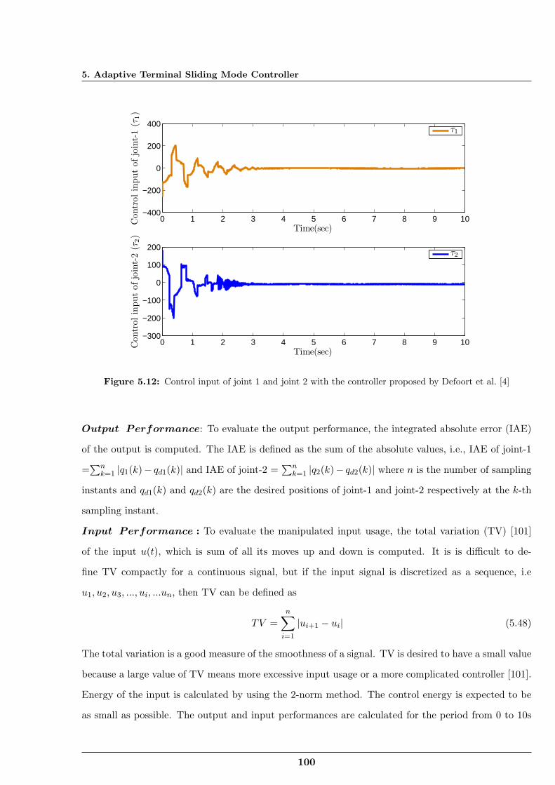
5. Adaptive Terminal Sliding Mode Controller
0 1 2 3 4 5 6 7 8 9 10−400
−200
0
200
400
Time(sec)
Contr
olin
put
ofjo
int-
1(τ
1)
τ1
0 1 2 3 4 5 6 7 8 9 10−300
−200
−100
0
100
200
Time(sec)
Contr
olin
put
ofjo
int-
2(τ
2)
τ2
Figure 5.12: Control input of joint 1 and joint 2 with the controller proposed by Defoort et al. [4]
Output Performance: To evaluate the output performance, the integrated absolute error (IAE)
of the output is computed. The IAE is defined as the sum of the absolute values, i.e., IAE of joint-1
=∑n
k=1 |q1(k)− qd1(k)| and IAE of joint-2 =∑n
k=1 |q2(k)− qd2(k)| where n is the number of sampling
instants and qd1(k) and qd2(k) are the desired positions of joint-1 and joint-2 respectively at the k-th
sampling instant.
Input Performance : To evaluate the manipulated input usage, the total variation (TV) [101]
of the input u(t), which is sum of all its moves up and down is computed. It is is difficult to de-
fine TV compactly for a continuous signal, but if the input signal is discretized as a sequence, i.e
u1, u2, u3, ..., ui, ...un, then TV can be defined as
TV =n∑i=1
|ui+1 − ui| (5.48)
The total variation is a good measure of the smoothness of a signal. TV is desired to have a small value
because a large value of TV means more excessive input usage or a more complicated controller [101].
Energy of the input is calculated by using the 2-norm method. The control energy is expected to be
as small as possible. The output and input performances are calculated for the period from 0 to 10s
100
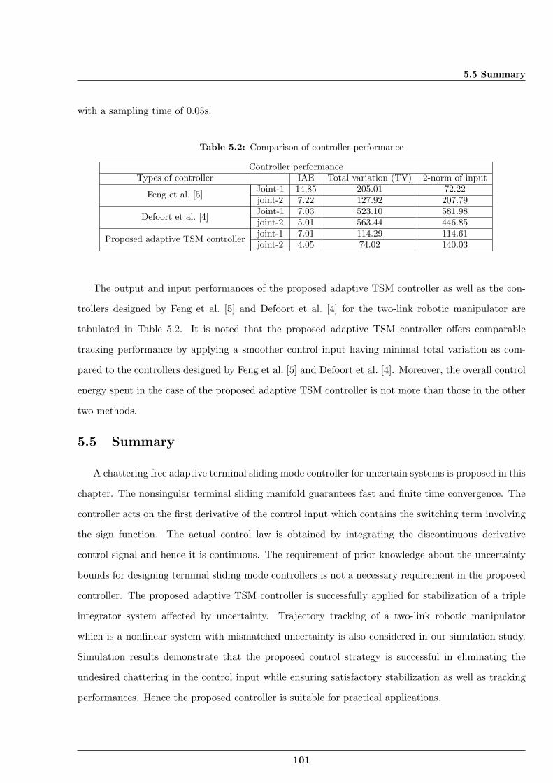
5.5 Summary
with a sampling time of 0.05s.
Table 5.2: Comparison of controller performance
Controller performanceTypes of controller IAE Total variation (TV) 2-norm of input
Feng et al. [5] Joint-1 14.85 205.01 72.22joint-2 7.22 127.92 207.79
Defoort et al. [4] Joint-1 7.03 523.10 581.98joint-2 5.01 563.44 446.85
Proposed adaptive TSM controller joint-1 7.01 114.29 114.61joint-2 4.05 74.02 140.03
The output and input performances of the proposed adaptive TSM controller as well as the con-
trollers designed by Feng et al. [5] and Defoort et al. [4] for the two-link robotic manipulator are
tabulated in Table 5.2. It is noted that the proposed adaptive TSM controller offers comparable
tracking performance by applying a smoother control input having minimal total variation as com-
pared to the controllers designed by Feng et al. [5] and Defoort et al. [4]. Moreover, the overall control
energy spent in the case of the proposed adaptive TSM controller is not more than those in the other
two methods.
5.5 Summary
A chattering free adaptive terminal sliding mode controller for uncertain systems is proposed in this
chapter. The nonsingular terminal sliding manifold guarantees fast and finite time convergence. The
controller acts on the first derivative of the control input which contains the switching term involving
the sign function. The actual control law is obtained by integrating the discontinuous derivative
control signal and hence it is continuous. The requirement of prior knowledge about the uncertainty
bounds for designing terminal sliding mode controllers is not a necessary requirement in the proposed
controller. The proposed adaptive TSM controller is successfully applied for stabilization of a triple
integrator system affected by uncertainty. Trajectory tracking of a two-link robotic manipulator
which is a nonlinear system with mismatched uncertainty is also considered in our simulation study.
Simulation results demonstrate that the proposed control strategy is successful in eliminating the
undesired chattering in the control input while ensuring satisfactory stabilization as well as tracking
performances. Hence the proposed controller is suitable for practical applications.
101
6Nonlinear Sliding Surface based
Adaptive Sliding Mode Controller
Contents
6.1 Introduction . . . . . . . . . . . . . . . . . . . . . . . . . . . . . . . . . . . . 103
6.2 Adaptive chattering free sliding mode (SM) controller using nonlinearsliding surface . . . . . . . . . . . . . . . . . . . . . . . . . . . . . . . . . . . 104
6.3 Composite nonlinear feedback based discrete integral sliding mode con-troller . . . . . . . . . . . . . . . . . . . . . . . . . . . . . . . . . . . . . . . . 121
6.4 Summary . . . . . . . . . . . . . . . . . . . . . . . . . . . . . . . . . . . . . . 136
102
6.1 Introduction
6.1 Introduction
In the previous chapters, stabilization and tracking problems of linear as well as nonlinear uncertain
systems were considered and attempts were made for their improvement using chattering free adaptive
sliding mode control which employed a linear sliding surface. In general, fast settling time and small
overshoot are the two important requirements in most of the design problems. However, it is well
known that quick response produces a large overshoot which is not at all desirable in many practical
electromechanical applications [102]. On the other hand, a low overshoot can be achieved at the cost
of a high settling time. However, a short settling time is also necessary for a quick response, but it
increases the overshoot. Thus the user has to choose between fast response and low overshoot and
most of the design problems make a trade-off between these two transient indices keeping the damping
ratio fixed.
This particular problem can be solved by using the composite nonlinear feedback (CNF) technique
[103–105]. CNF method uses a variable damping ratio to achieve high transient performance. Initially,
the damping ratio is chosen as a very low value to ensure quick response and as the output approaches
the reference, the damping ratio is increased to reduce the overshoot.In [6, 67, 106, 107], the CNF
method was used to design a nonlinear sliding surface which increased the damping ratio from its
initial low value as the output approached the set point. This resulted in a fast response at the
beginning and gradually as the output approached the set point, the effect was to reduce the settling
time and overshoot.
This chapter focuses to improve the transient performance of an uncertain system by developing a
chattering free sliding mode controller which uses a nonlinear sliding surface. Here a proportional
plus constant reaching law based chattering free sliding mode controller is proposed using nonlinear
sliding surface to improve the transient performance. An adaptive tuning law is used to deal with
unknown but bounded system uncertainties. Further, a discrete integral sliding mode controller based
on nonlinear sliding surface is designed to investigate the performance in the discrete domain.
This chapter is organized as follows:
The proposed adaptive sliding mode (SM) controller using nonlinear sliding surface is discussed in
Section 6.2. Section 6.3 discusses about nonlinear sliding surface based discrete integral sliding mode
controller for uncertain systems. A brief summary is presented in Section 6.4.
103
6. Nonlinear Sliding Surface based Adaptive Sliding Mode Controller
6.2 Adaptive chattering free sliding mode (SM) controller usingnonlinear sliding surface
A class of dynamic system is considered as follows,
x = f(x) + g(x)u
y = σ(x) (6.1)
where x ∈ Rn is the state variable, u ∈ Rm is the control input, y ∈ R is the output and σ(x) ∈ R
is the measured output function known as the sliding variable. Moreover, f(x) and g(x) are smooth
functions.
Using appropriate transformation, the above nonlinear system (6.1) can be transformed into the
following Brunowsky canonical form [106],
xi = xi+1 i = 1, ..., (n− 1)
xn = an1x1 + an2x2 + .....+ annxn +Bnu+Bnfm(x, t) (6.2)
The above system can be expressed as,
x = Ax+B(u+ fm(x, t))
y1 = C1x (6.3)
where x ∈ Rn is the state vector, u ∈ Rm is the control input, y1 is the output and fm(x, t) ∈ Rm rep-
resents parametric perturbation and external disturbances and is assumed to be matched. Here A, B
and C1 are known matrices with proper dimensions and n, m are also known. The system (6.3) can be
transformed into regular form by using a transformation matrix Tr [106], such that z = Trx = [z1 z2]T .
Then the following transformed system is obtained,
z1 = a11z1 + a12z2
z2 = a21z1 + a22z2 +B2u+B2fm(z, t)
y1 = Cz1 (6.4)
104
6.2 Adaptive chattering free sliding mode (SM) controller using nonlinear sliding surface
Here, z1 ∈ Rn−1, z2 ∈ R and C = C1(Tr)−1.
From (6.4) the following can be written,
z = Aregz +Bu+Bfm(z, t) (6.5)
where fm(z, t) contains all the uncertain terms along with disturbances and Areg can be expressed as,
Areg =[a11 a12
a21 a22
]B = [0 B2]T (6.6)
The nonlinear sliding surface is selected as [106],
cT (t) = [F − Υ(r, y)aT12P 1] (6.7)
where Υ(r, y) is a negative nonlinear function and F is a real matrix. Then
s = cT (t)e= [F − Υ(r, y)aT12P 1]e (6.8)
where e = [e1 e2]T = [z1−z1d z2−z2d]T and zd = [z1d z2d]T is the desired state. Here F is chosen
such that (a11−a12F ) has stable poles and the dominant poles have low damping ratio. Furthermore,
Υ(r, y) is a negative nonlinear function which raises its value starting with zero such that the damping
ratio for the overall system increases from an initial low value to higher ones [67,106]. Moreover, P is
a positive definite matrix which can be found by solving the Lyapunov criterion given by,
(a11 − a12F )TP + P (a11 − a12F ) = −R (6.9)
where R is also a positive definite matrix.
6.2.1 Stability in sliding mode
During the sliding mode, s = 0 and hence from (6.8)
e2 = −Fe1 + Υ(r, y)aT12Pe1 (6.10)
105
6. Nonlinear Sliding Surface based Adaptive Sliding Mode Controller
Using (6.5) and (6.10) yields
e1 = (a11 − a12F + a12Υ(r, y)aT12P )e1 + h (6.11)
where h = a11z1d + a12z2d − z1d. Suppose that the desired trajectory zd is consistently generated by
using the system model. Then there exists some control u such that
z1d = a11z1d + a12z2d
z2d = a21z1d + a22z2d +B2u (6.12)
Using (6.11) and (6.12) yields,
e1 = (a11 − a12F + a12Υ(r, y)aT12P )e1 (6.13)
To prove the stability in the sliding mode, let us consider the following Lyapunov function,
V1 = eT1 Pe1
Taking its derivative and using (6.13) yields
V1 = eT1 Pe1 + eT1 P e1
= eT1 (a11 − a12F )TPe1 + eT1 P (a11 − a12F )e1 + 2eT1 Pa12Υ(r, y)aT12Pe1
= eT1 [(a11 − a12F )TP + P (a11 − a12F )]e1 + 2eT1 Pa12Υ(r, y)aT12Pe1
= eT1 [(a11 − a12F )TP + P (a11 − a12F ) + 2Pa12Υ(r, y)aT12P ]e1
= eT1 [−R+ 2Pa12Υ(r, y)aT12P ]e1
Let there exist a matrix Q = eT1 Pa12. Thus V1 can be simplified as,
V1 = −eT1Re1 + 2QΥ(r, y)QT
Since R > 0 and Υ(r, y) < 0,
V1 < 0 (6.14)
Thus stability in sliding mode is proved. Taking first derivative of s and using (6.8) and (6.5), the
following is obtained:
s = cT (t)z − cT (t)zd − cT (t)zd + cT (t)(Aregz +Bu+Bfm(z, t)) (6.15)
106
6.2 Adaptive chattering free sliding mode (SM) controller using nonlinear sliding surface
Taking the second derivative of s yields
s = cT (t)z + cT (t)z + cT (t)Areg z + cT (t)Aregz + cT (t)Bu+ cT (t)Bu
+cT (t)Bfm(z, t) + cT (t)Bfm(z, t) − d
dt(cT (t)zd + cT (t)zd)
= cT (t)A2regz + 2cT (t)Aregz + cT (t)z + cT (t)AregBu
+2cT (t)Bu+ cT (t)B2u− cT (t)zd − cT (t)zd − cT (t)zd
−cT (t)zd + cT (t)AregBfm(z, t) + 2cT (t)Bfm(z, t) + cT (t)Bfm(z, t) (6.16)
Let all the uncertainties be norm bounded and
(cT (t)AregBfm(z, t) + 2cT (t)Bfm(z, t) + cT (t)Bfm(z, t)) = ∆F (z, t).
Assuming y1(z) = s and y2(z) = s, the system dynamics can be written as,
y1(z) = y2(z)
y2(z) = Φ(z, u) + Ψ(z)v (6.17)
where v = u and Φ(z, u) collects all the uncertain terms not involving u. Thus the systems (6.15) and
(6.16) are now controlled by the input v. A sliding mode controller can be designed for the above
system using the control input v to keep the system trajectories in the sliding manifold.
Let the sliding manifold be considered as,
σ = y2(z) + κy1(z) (6.18)
where κ is a positive constant.
Taking the derivative of (6.18) yields,
σ = y2(z) + κy1(z) (6.19)
Using (6.15) and (6.16), the following is obtained,
σ = cT (t)A2regz + 2cT (t)Aregz + cT (t)z + cT (t)AregBu
+ 2cT (t)Bu+ cT (t)Bu− cT (t)zd − cT (t)zd − cT (t)zd
− cT (t)zd + κs+ ∆F (z, t) (6.20)
107
6. Nonlinear Sliding Surface based Adaptive Sliding Mode Controller
Using the constant plus proportional reaching law yields,
σ = −k1σ − k2sign(σ) (6.21)
Using (6.20) and (6.21), the control law is obtained as,
u = −(cT (t)B)−1[cT (t)A2regz + 2cT (t)Aregz + cT (t)z
+ cT (t)AregBu+ 2cT (t)Bu− cT (t)zd − cT (t)zd − cT (t)zd
− cT (t)zd + k1σ + k2sign(σ) + κs] (6.22)
where k1 ≥ 0 and k2 > |(cT (t)AregBfm(z, t) + 2cT (t)Bfm(z, t) + cT (t)Bfm(z, t))| = |∆F (z, t)| to
satisfy the reaching law condition σσ ≤ −η|σ| for some η > 0.
In practice, the upper bound of the system uncertainty is often unknown in advance and hence the
error term |∆F (z, t)| is difficult to find. An adaptive tuning law is proposed to estimate k2 using
which the control law (6.22) can be written as
u = −(cT (t)B)−1[cT (t)A2regz + 2cT (t)AregBz + cT (t)z
+ cT (t)AregBu+ 2cT (t)Bu− cT (t)zd − cT (t)zd − cT (t)zd
− cT (t)zd + k1σ + T sign(σ) + κs] (6.23)
where T estimates the value of k2. Defining the adaptation error as T = T − T , the parameter T is
estimated by using the adaptation law as in (4.57) [40,69,70,108] and given below,
˙T = ν|σ| (6.24)
where ν is a positive constant. A Lyapunov function V2 is selected as V2 = 12σ
2 + 12γT
2 whose time
derivative is as follows,
V2 = σσ + γT ˙TUsing (6.20) yields,
V2 = σ[cT (t)A2regz + 2cT (t)Aregz + cT (t)z + cT (t)AregBu
108
6.2 Adaptive chattering free sliding mode (SM) controller using nonlinear sliding surface
+ 2cT (t)Bu+ cT (t)Bu− cT (t)zd − cT (t)zd − cT (t)zd − cT (t)zd
+ κs+ ∆F (z, t)] + γ(T − T ) ˙T
Using (6.23) and (6.24) yields,V2 = σ[∆F (z, t) − T sign(σ) − k1σ] + γ(T − T )ν|σ|
Since k1 ≥ 0, the above equation can be written asV2 ≤| ∆F (z, t) | |σ| − T |σ| + T |σ| − T |σ| + γ(T − T )ν|σ|
≤ (|∆F (z, t)| − T )|σ| − (T − T )|σ| + γ(T − T )ν|σ|≤ −(−|∆F (z, t)| + T )|σ| − (T − T )(−γν|σ| + |σ|)≤ −βσ
√2|σ/
√2| − βν
√γ/2(T − T )/
√γ/2
where βσ = (T − |∆F (z, t)|) and βν = (|σ| − γν|σ|)So, V2 ≤ −minβσ
√2, βν
√2/γ(|σ/
√2| + T
√γ/2)
≤ −βV 1/22 (6.25)
where β = minβσ√
2, βν√
2/γ with β > 0. The above inequality holds if ˙T = ν|σ|, βσ > 0, βν >
0, T > |∆F (z, t)| and γ < 1ν . Therefore, finite time convergence to a domain σ = 0 is guaranteed
from any initial condition [40,62]. The adaptive tuning law (6.24) is modified by using the dead zone
technique.
It is evident from (6.23) that u is discontinuous but integration of u yields a continuous control law
u. Hence the undesired high frequency chattering of the control signal is eliminated. Thus the above
adaptive SM control with nonlinear sliding surface offers following advantages. Firstly, an improved
transient performance can be obtained without the knowledge about the upper bound of the system
uncertainties. Secondly, the chattering in the control input is eliminated.
Assumption 6.1. An exact robust differentiator is available for exactly measuring or estimating the
derivative of variables.
6.2.2 Choice of nonlinear function Υ(r, y)
The nonlinear function Υ(r, y) is used to change the system’s damping ratio as the output y
approaches the reference position r [104] [67]. It possesses the properties mentioned below:
• When the output is far from the reference value, Υ(r, y) equals to zero (or a very small value).
• As the output approaches its final desired value, Υ(r, y) value gradually becomes highly negative.
• The nonlinear function Υ(r, y) should be continuous, differentiable and its higher derivatives
must exist.
109
6. Nonlinear Sliding Surface based Adaptive Sliding Mode Controller
The choice of Υ(r, y) is not unique. Some examples of Υ(r, y) used in literature are discussed below
[102].
Υ(r, y) = −ϱe−ψ(y−r)2 (6.26)
where r and y are the reference input and the system output respectively. Here ϱ > 0, ψ > 0 are
the tuning parameters. It is observed that the nonlinear function decreases its value from 0 to −ϱ as
the value of error (y − r) decreases from infinity (very high value) to zero. Another type of nonlinear
function Υ(r, y) used is given by,
Υ(r, y) = −ϱe−ψ|y−r| (6.27)
The value of Υ(r, y) changes from 0 to −ϱ as the error (y− r) approaches zero [109] from a high value.
Υ(r, y) can assume the following form also,
Υ(r, y) = − ϱ
1 − e−1(e−(1−(y−y0)/(r−y0))2 − e−1) (6.28)
where r is the reference input, y0 = y(0) is the initial state and ϱ is the tuning parameter. The
function Υ(r, y) changes its value from 0 to −ϱ as the error (y− r) approaches zero from a high value.
6.2.3 Simulation Results
The proposed controller is simulated in MATLAB-Simulink by using ODE 8 solver with a fixed
step size of 0.005 sec.
6.2.3.1 Time response of second order process with time delay
The proposed adaptive SM controller is applied to a second order uncertain system with time delay.
The performance of the proposed adaptive SM controller using nonlinear sliding surface is compared
with that obtained by using adaptive SM controller with different linear sliding surfaces. The second
order process with time delay is given by [9]
G(s) =0.05e−0.5s
(1 + 0.1s)(1 + s)(6.29)
which can be simplified to the following form using Pade approximation,
G(s) =0.05
(1 + 0.5s)(1 + 0.1s)(1 + s)(6.30)
110
6.2 Adaptive chattering free sliding mode (SM) controller using nonlinear sliding surface
The state space model given by Eq.(6.3) is obtained with
A =
0 1 00 0 1
−20 −32 −13
, B =
001
, C1 = [ 1 0 0 ] (6.31)
The matched uncertainty considered here is fm(x, t) = 0.5sin(10t).
Since the system is already in the regular form, the following submatrices can be written,
z1 = [x1 x2]T , z2 = x3 and coefficient matrices
a11 =[
0 10 0
], a12 =
[01
]a21 =
[−20 −32
], a22 = −13, B2 = 1, C = C1 (6.32)
• Design of nonlinear sliding surface:
The nonlinear sliding surface consists of a linear and a nonlinear term. Initially, the nonlinear term
has a very low value and as the system gradually approaches its desired position, the nonlinear term
decreases its value to a high negative value and thereby changes the value of the damping ratio. As a
result, the system response has low overshoot and small settling time. Let us recall,
cT (t) = [F − Υ(r, y)aT12P 1] (6.33)
Here the gain matrix F is designed for low damping ratio and high setting time. Moreover, F can be
designed by using pole placement technique. Let initially the system have damping ratio ξ1 and settling
time ts1. The closed loop poles are located at (−ξ1ωn +√
(ξ21 − 1)ωn) and (−ξ1ωn −√
(ξ21 − 1)ωn).
The natural frequency of oscillations ωn is given by,
ωn =4
ξ1ts1(6.34)
Let us choose the initial damping ratio ξ1 = 0.4 and settling time ts1 = 3.5. Using (6.34), the poles
can be found to be located at −1.1429 + 2.6186i,−1.1429 − 2.6186i. Thus F can be calculated using
pole placement technique as F = [8.1633 2.2857]. Solution of the Lyapunov equation (6.9) yields,
P =[
0.2144 0.00610.0061 0.0246
]using R =
[0.1 00 0.1
](6.35)
111
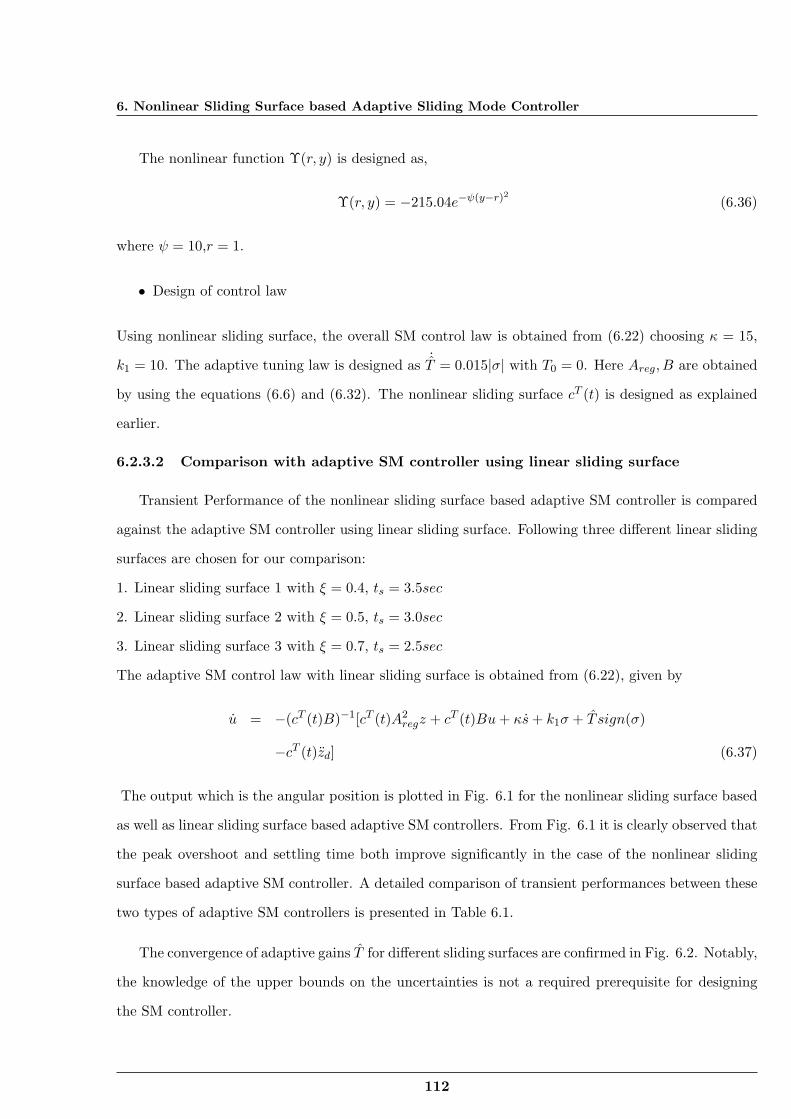
6. Nonlinear Sliding Surface based Adaptive Sliding Mode Controller
The nonlinear function Υ(r, y) is designed as,
Υ(r, y) = −215.04e−ψ(y−r)2 (6.36)
where ψ = 10,r = 1.
• Design of control law
Using nonlinear sliding surface, the overall SM control law is obtained from (6.22) choosing κ = 15,
k1 = 10. The adaptive tuning law is designed as ˙T = 0.015|σ| with T0 = 0. Here Areg, B are obtained
by using the equations (6.6) and (6.32). The nonlinear sliding surface cT (t) is designed as explained
earlier.
6.2.3.2 Comparison with adaptive SM controller using linear sliding surface
Transient Performance of the nonlinear sliding surface based adaptive SM controller is compared
against the adaptive SM controller using linear sliding surface. Following three different linear sliding
surfaces are chosen for our comparison:
1. Linear sliding surface 1 with ξ = 0.4, ts = 3.5sec
2. Linear sliding surface 2 with ξ = 0.5, ts = 3.0sec
3. Linear sliding surface 3 with ξ = 0.7, ts = 2.5sec
The adaptive SM control law with linear sliding surface is obtained from (6.22), given by
u = −(cT (t)B)−1[cT (t)A2regz + cT (t)Bu+ κs+ k1σ + T sign(σ)
−cT (t)zd] (6.37)
The output which is the angular position is plotted in Fig. 6.1 for the nonlinear sliding surface based
as well as linear sliding surface based adaptive SM controllers. From Fig. 6.1 it is clearly observed that
the peak overshoot and settling time both improve significantly in the case of the nonlinear sliding
surface based adaptive SM controller. A detailed comparison of transient performances between these
two types of adaptive SM controllers is presented in Table 6.1.
The convergence of adaptive gains T for different sliding surfaces are confirmed in Fig. 6.2. Notably,
the knowledge of the upper bounds on the uncertainties is not a required prerequisite for designing
the SM controller.
112
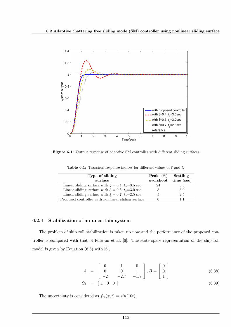
6.2 Adaptive chattering free sliding mode (SM) controller using nonlinear sliding surface
0 1 2 3 4 5 6 7 8 9 100
0.2
0.4
0.6
0.8
1
1.2
1.4
Time(sec)
Sys
tem
out
put
with proposed controllerwith ξ=0.4, t
s=3.5sec
with ξ=0.5, ts=3.0sec
with ξ=0.7, ts=2.5sec
reference
Figure 6.1: Output response of adaptive SM controller with different sliding surfaces
Table 6.1: Transient response indices for different values of ξ and ts
Type of sliding Peak (%) Settlingsurface overshoot time (sec)
Linear sliding surface with ξ = 0.4, ts=3.5 sec 24 3.5Linear sliding surface with ξ = 0.5, ts=3.0 sec 8 3.0Linear sliding surface with ξ = 0.7, ts=2.5 sec 5 2.5
Proposed controller with nonlinear sliding surface 0 1.1
6.2.4 Stabilization of an uncertain system
The problem of ship roll stabilization is taken up now and the performance of the proposed con-
troller is compared with that of Fulwani et al. [6]. The state space representation of the ship roll
model is given by Equation (6.3) with [6],
A =
0 1 00 0 1−2 −2.7 −1.7
, B =
001
(6.38)
C1 = [ 1 0 0 ] (6.39)
The uncertainty is considered as fm(x, t) = sin(10t).
113
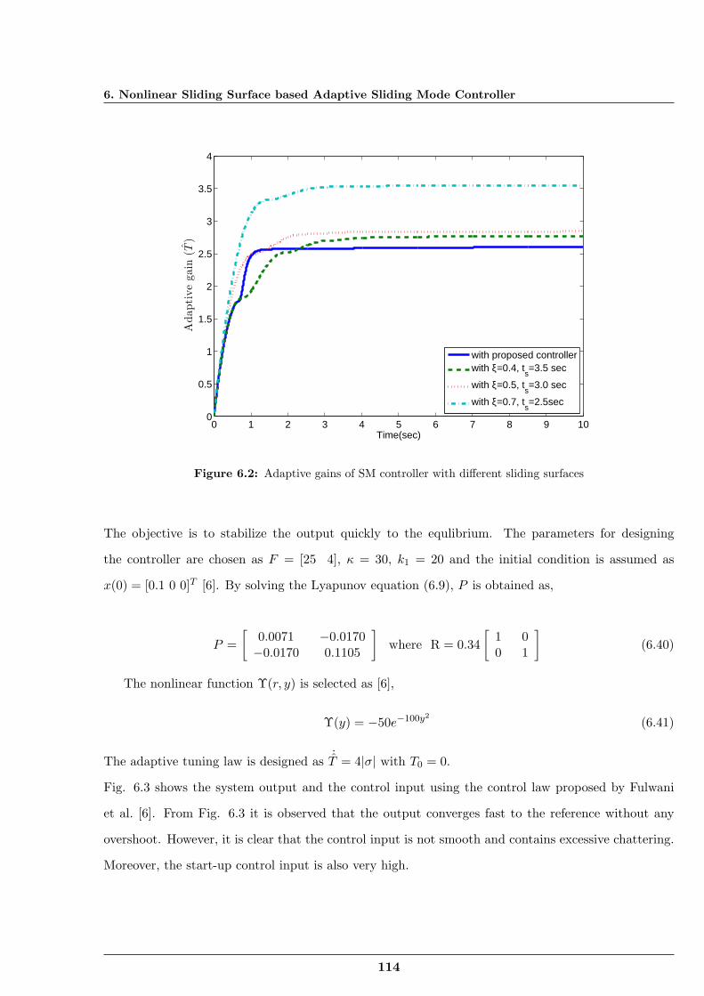
6. Nonlinear Sliding Surface based Adaptive Sliding Mode Controller
0 1 2 3 4 5 6 7 8 9 100
0.5
1
1.5
2
2.5
3
3.5
4
Time(sec)
Adapti
ve
gain
(T)
with proposed controllerwith ξ=0.4, t
s=3.5 sec
with ξ=0.5, ts=3.0 sec
with ξ=0.7, ts=2.5sec
Figure 6.2: Adaptive gains of SM controller with different sliding surfaces
The objective is to stabilize the output quickly to the equlibrium. The parameters for designing
the controller are chosen as F = [25 4], κ = 30, k1 = 20 and the initial condition is assumed as
x(0) = [0.1 0 0]T [6]. By solving the Lyapunov equation (6.9), P is obtained as,
P =[
0.0071 −0.0170−0.0170 0.1105
]where R = 0.34
[1 00 1
](6.40)
The nonlinear function Υ(r, y) is selected as [6],
Υ(y) = −50e−100y2 (6.41)
The adaptive tuning law is designed as ˙T = 4|σ| with T0 = 0.
Fig. 6.3 shows the system output and the control input using the control law proposed by Fulwani
et al. [6]. From Fig. 6.3 it is observed that the output converges fast to the reference without any
overshoot. However, it is clear that the control input is not smooth and contains excessive chattering.
Moreover, the start-up control input is also very high.
114
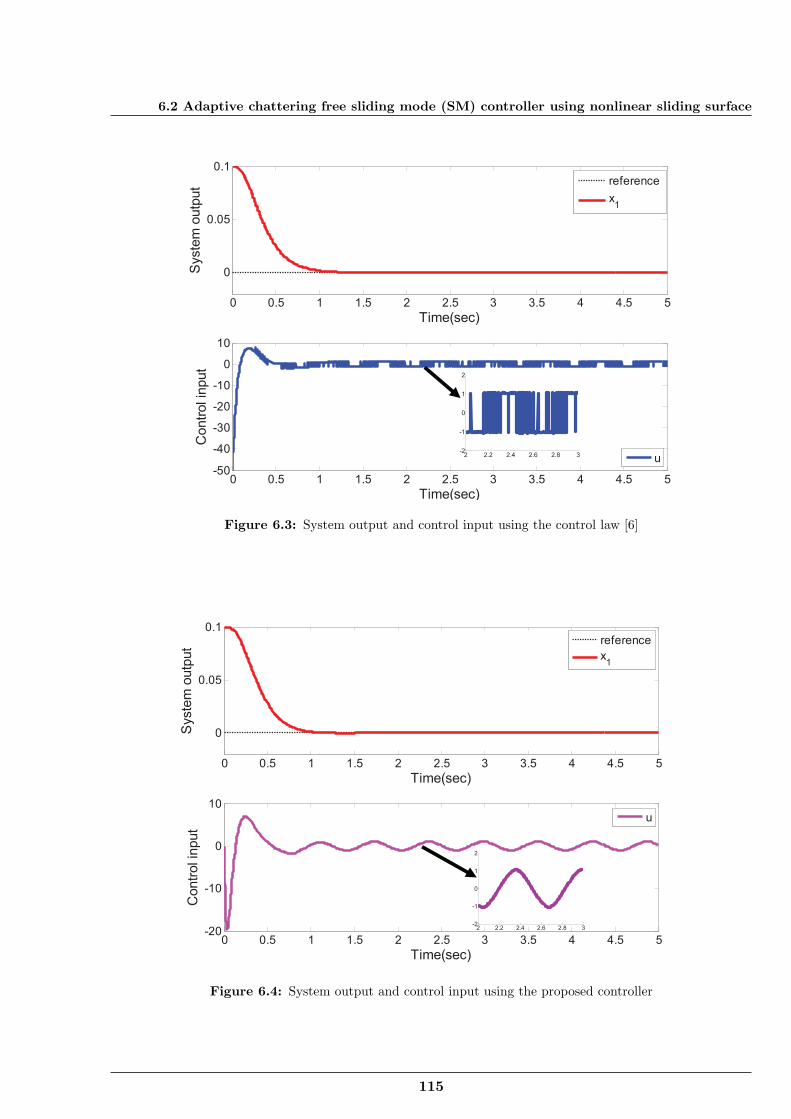
6.2 Adaptive chattering free sliding mode (SM) controller using nonlinear sliding surface
0 0.5 1 1.5 2 2.5 3 3.5 4 4.5 5
0
0.05
0.1
Time(sec)
Syste
m o
utp
ut reference
x1
0 0.5 1 1.5 2 2.5 3 3.5 4 4.5 5-50
-40
-30
-20
-10
0
10
Time(sec)
Contr
ol in
put
u2 2.2 2.4 2.6 2.8 3-2
-1
0
1
2
Figure 6.3: System output and control input using the control law [6]
0 0.5 1 1.5 2 2.5 3 3.5 4 4.5 5
0
0.05
0.1
Time(sec)
Syste
m o
utp
ut
reference
x1
0 0.5 1 1.5 2 2.5 3 3.5 4 4.5 5-20
-10
0
10
Time(sec)
Contr
ol in
put
u
2 2.2 2.4 2.6 2.8 3-2
-1
0
1
2
Figure 6.4: System output and control input using the proposed controller
115
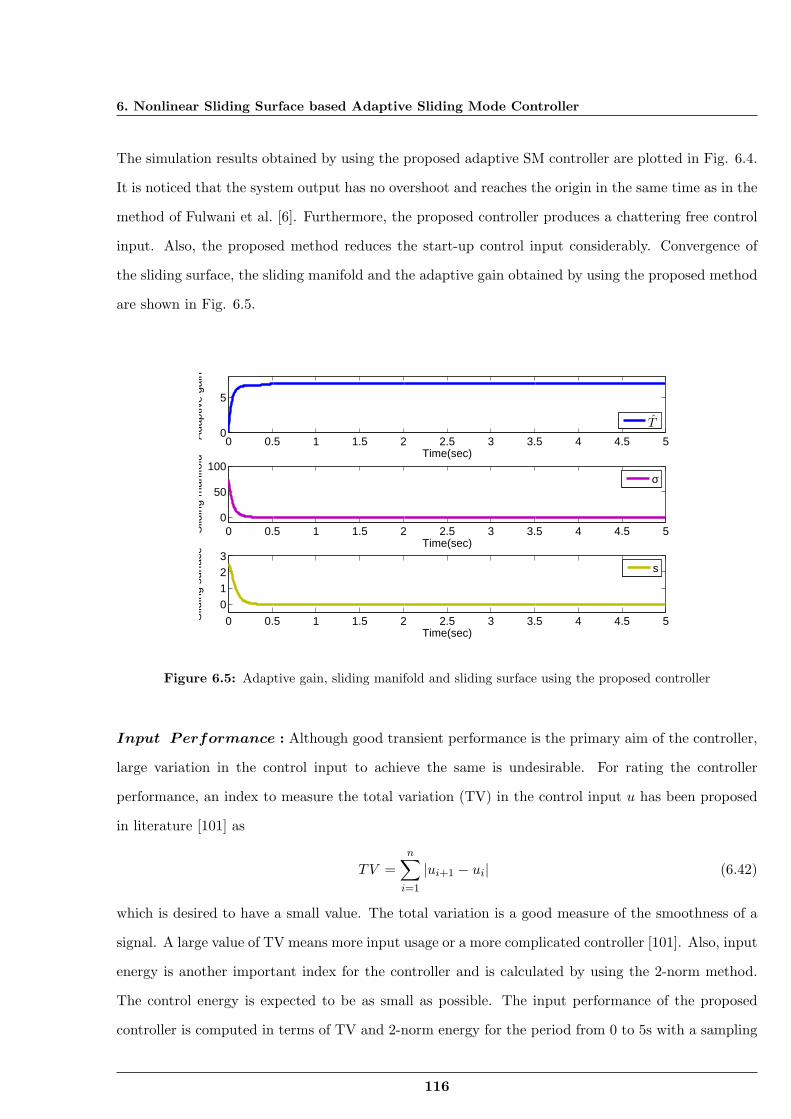
6. Nonlinear Sliding Surface based Adaptive Sliding Mode Controller
The simulation results obtained by using the proposed adaptive SM controller are plotted in Fig. 6.4.
It is noticed that the system output has no overshoot and reaches the origin in the same time as in the
method of Fulwani et al. [6]. Furthermore, the proposed controller produces a chattering free control
input. Also, the proposed method reduces the start-up control input considerably. Convergence of
the sliding surface, the sliding manifold and the adaptive gain obtained by using the proposed method
are shown in Fig. 6.5.
0 0.5 1 1.5 2 2.5 3 3.5 4 4.5 50
5
Time(sec)
Ada
ptiv
e ga
in
T
0 0.5 1 1.5 2 2.5 3 3.5 4 4.5 50
50
100
Time(sec)
Slid
ing
man
ifold
σ
0 0.5 1 1.5 2 2.5 3 3.5 4 4.5 5
0123
Time(sec)
Slid
ing
surf
ace
s
Figure 6.5: Adaptive gain, sliding manifold and sliding surface using the proposed controller
Input Performance : Although good transient performance is the primary aim of the controller,
large variation in the control input to achieve the same is undesirable. For rating the controller
performance, an index to measure the total variation (TV) in the control input u has been proposed
in literature [101] as
TV =n∑i=1
|ui+1 − ui| (6.42)
which is desired to have a small value. The total variation is a good measure of the smoothness of a
signal. A large value of TV means more input usage or a more complicated controller [101]. Also, input
energy is another important index for the controller and is calculated by using the 2-norm method.
The control energy is expected to be as small as possible. The input performance of the proposed
controller is computed in terms of TV and 2-norm energy for the period from 0 to 5s with a sampling
116
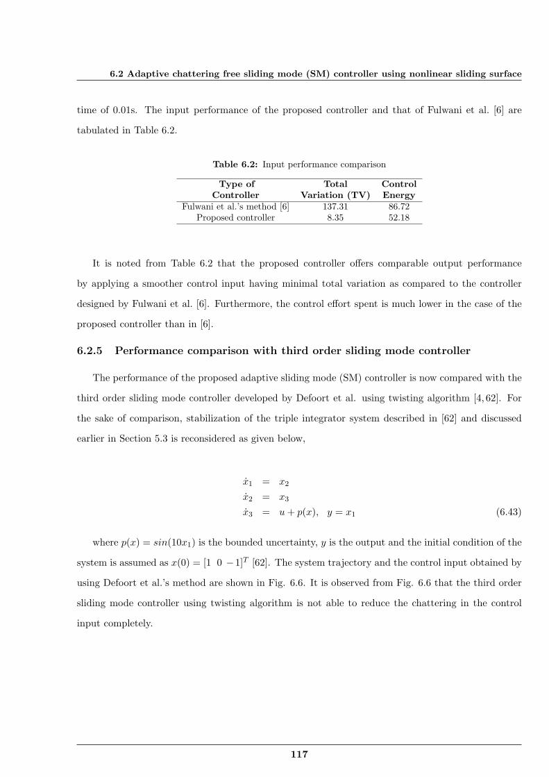
6.2 Adaptive chattering free sliding mode (SM) controller using nonlinear sliding surface
time of 0.01s. The input performance of the proposed controller and that of Fulwani et al. [6] are
tabulated in Table 6.2.
Table 6.2: Input performance comparison
Type of Total ControlController Variation (TV) Energy
Fulwani et al.’s method [6] 137.31 86.72Proposed controller 8.35 52.18
It is noted from Table 6.2 that the proposed controller offers comparable output performance
by applying a smoother control input having minimal total variation as compared to the controller
designed by Fulwani et al. [6]. Furthermore, the control effort spent is much lower in the case of the
proposed controller than in [6].
6.2.5 Performance comparison with third order sliding mode controller
The performance of the proposed adaptive sliding mode (SM) controller is now compared with the
third order sliding mode controller developed by Defoort et al. using twisting algorithm [4, 62]. For
the sake of comparison, stabilization of the triple integrator system described in [62] and discussed
earlier in Section 5.3 is reconsidered as given below,
x1 = x2
x2 = x3
x3 = u+ p(x), y = x1 (6.43)
where p(x) = sin(10x1) is the bounded uncertainty, y is the output and the initial condition of the
system is assumed as x(0) = [1 0 −1]T [62]. The system trajectory and the control input obtained by
using Defoort et al.’s method are shown in Fig. 6.6. It is observed from Fig. 6.6 that the third order
sliding mode controller using twisting algorithm is not able to reduce the chattering in the control
input completely.
117
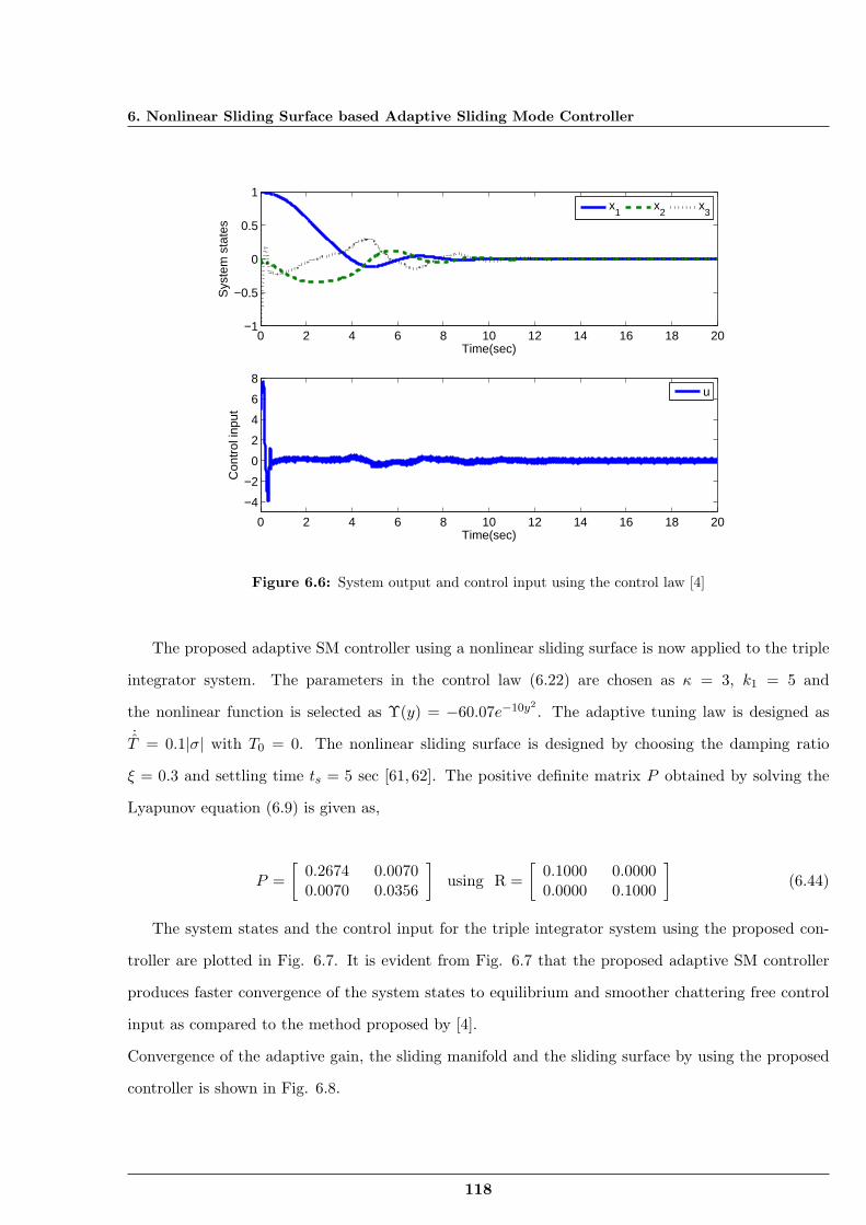
6. Nonlinear Sliding Surface based Adaptive Sliding Mode Controller
0 2 4 6 8 10 12 14 16 18 20−1
−0.5
0
0.5
1
Time(sec)
Sys
tem
sta
tes
x1
x2
x3
0 2 4 6 8 10 12 14 16 18 20
−4
−2
0
2
4
6
8
Time(sec)
Con
trol
inpu
t
u
Figure 6.6: System output and control input using the control law [4]
The proposed adaptive SM controller using a nonlinear sliding surface is now applied to the triple
integrator system. The parameters in the control law (6.22) are chosen as κ = 3, k1 = 5 and
the nonlinear function is selected as Υ(y) = −60.07e−10y2 . The adaptive tuning law is designed as˙T = 0.1|σ| with T0 = 0. The nonlinear sliding surface is designed by choosing the damping ratio
ξ = 0.3 and settling time ts = 5 sec [61, 62]. The positive definite matrix P obtained by solving the
Lyapunov equation (6.9) is given as,
P =[
0.2674 0.00700.0070 0.0356
]using R =
[0.1000 0.00000.0000 0.1000
](6.44)
The system states and the control input for the triple integrator system using the proposed con-
troller are plotted in Fig. 6.7. It is evident from Fig. 6.7 that the proposed adaptive SM controller
produces faster convergence of the system states to equilibrium and smoother chattering free control
input as compared to the method proposed by [4].
Convergence of the adaptive gain, the sliding manifold and the sliding surface by using the proposed
controller is shown in Fig. 6.8.
118
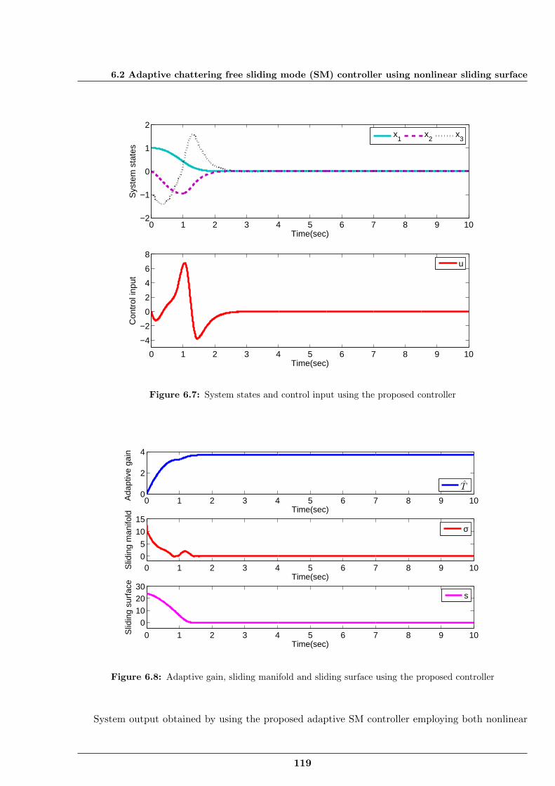
6.2 Adaptive chattering free sliding mode (SM) controller using nonlinear sliding surface
0 1 2 3 4 5 6 7 8 9 10−2
−1
0
1
2
Time(sec)
Sys
tem
sta
tes
x1
x2
x3
0 1 2 3 4 5 6 7 8 9 10
−4
−2
0
2
4
6
8
Time(sec)
Con
trol
inpu
t
u
Figure 6.7: System states and control input using the proposed controller
0 1 2 3 4 5 6 7 8 9 100
2
4
Time(sec)
Ada
ptiv
e ga
in
T
0 1 2 3 4 5 6 7 8 9 100
5
10
15
Time(sec)
Slid
ing
man
ifold
σ
0 1 2 3 4 5 6 7 8 9 10
0102030
Time(sec)
Slid
ing
surf
ace
s
Figure 6.8: Adaptive gain, sliding manifold and sliding surface using the proposed controller
System output obtained by using the proposed adaptive SM controller employing both nonlinear
119
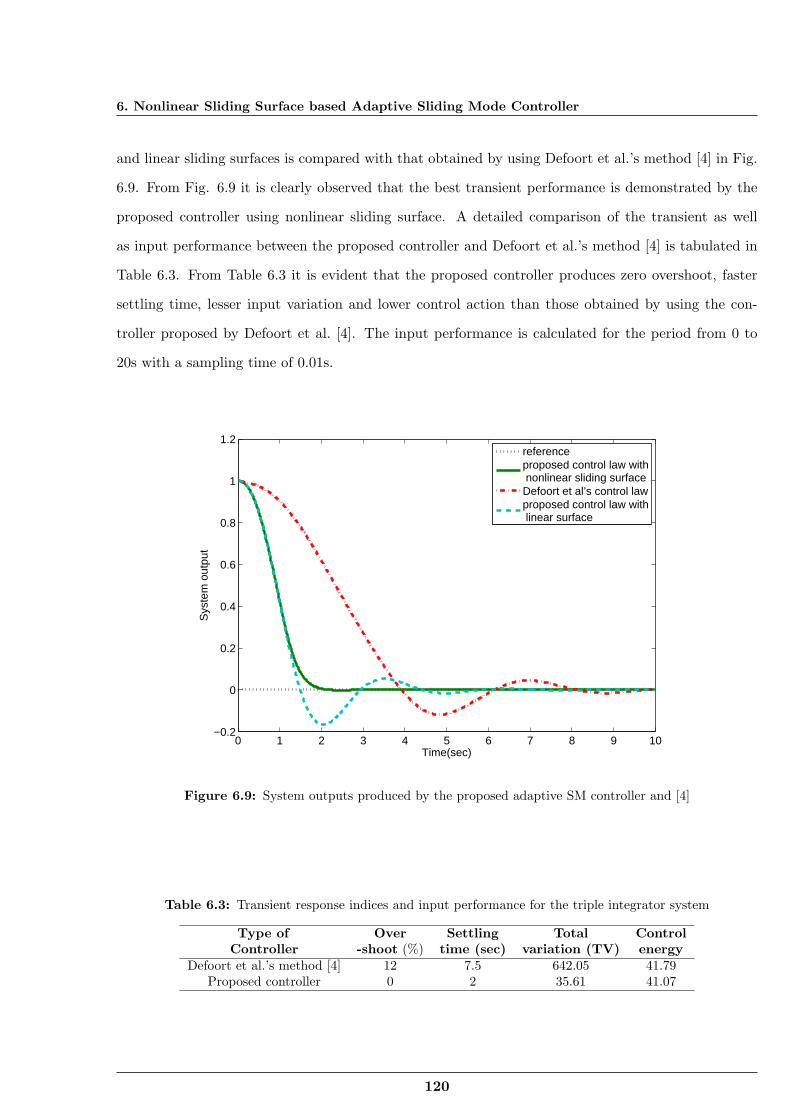
6. Nonlinear Sliding Surface based Adaptive Sliding Mode Controller
and linear sliding surfaces is compared with that obtained by using Defoort et al.’s method [4] in Fig.
6.9. From Fig. 6.9 it is clearly observed that the best transient performance is demonstrated by the
proposed controller using nonlinear sliding surface. A detailed comparison of the transient as well
as input performance between the proposed controller and Defoort et al.’s method [4] is tabulated in
Table 6.3. From Table 6.3 it is evident that the proposed controller produces zero overshoot, faster
settling time, lesser input variation and lower control action than those obtained by using the con-
troller proposed by Defoort et al. [4]. The input performance is calculated for the period from 0 to
20s with a sampling time of 0.01s.
0 1 2 3 4 5 6 7 8 9 10−0.2
0
0.2
0.4
0.6
0.8
1
1.2
Time(sec)
Sys
tem
out
put
referenceproposed control law with nonlinear sliding surfaceDefoort et al’s control lawproposed control law with linear surface
Figure 6.9: System outputs produced by the proposed adaptive SM controller and [4]
Table 6.3: Transient response indices and input performance for the triple integrator system
Type of Over Settling Total ControlController -shoot (%) time (sec) variation (TV) energy
Defoort et al.’s method [4] 12 7.5 642.05 41.79Proposed controller 0 2 35.61 41.07
120
6.3 Composite nonlinear feedback based discrete integral sliding mode controller
6.3 Composite nonlinear feedback based discrete integral slidingmode controller
The use of digital computers and samplers in the control circuitry in the recent years has made
the use of discrete time system representation more justifiable for controller design than continuous
time representation. As such study and research on discrete sliding mode has received wide attention
[57] [110] [111] [112] [113] [114]. To analyze the effect of sampling time, discrete time sliding mode
control (DSMC) is well studied in the literature [7] [115] [116] [117] [118]. In this section, a nonlinear
feedback based discrete integral sliding mode controller is proposed for uncertain systems with matched
uncertainty.
The main idea behind the integral sliding mode (ISM) controller is to design the control law as a
sum of a nominal control and a discontinuous control. Nominal control takes care of the nominal
plant dynamics and the discontinuous ISM control rejects disturbances. Here the composite nonlinear
feedback (CNF) controller, which is based on variable damping ratio, is used as the nominal controller
to achieve good transient performance and the discrete integral sliding mode (ISM) controller is
combined to ensure invariance against disturbances [114].
6.3.1 Discrete ISM controller for linear system with matched uncertainty
Let us consider a continuous time linear uncertain system as given below,
x = Ax+B(u+ fm(x, t))
y = Cx (6.45)
where x ∈ Rn is the state vector, u ∈ Rm is the control input and y ∈ Rp is the output vector. The
matrices A, B, C and dimensions n, m, p are known apriori. Furthermore, fm(x, t) is the matched
uncertainty caused by unmodeled dynamics and external disturbance.
Let the above continuous system be sampled at τ samples per second, assuming that the distur-
bance is slowly varying. The discrete equivalent of the above plant (6.45) is then given by [119],
x(k + 1) = ϕτx(k) + Γτu(k) + d(k)
y(k) = Cx(k) (6.46)
121
6. Nonlinear Sliding Surface based Adaptive Sliding Mode Controller
where the matrices ϕτ , Γτ , C are of appropriate dimensions and d(k) is the matched uncertainty.
The above matrices are defined as follows [119],
ϕτ = eAτ
Γτ =
τ∫0
eAtBdt
d(k) =
τ∫0
eAtBfm((k + 1)τ − t)dt (6.47)
For a smooth bounded disturbance fm(t) [7],
d(k) =
τ∫0
eAtBfm((k + 1)τ − t)dt
= Γτfm(k) +12Γτvm(k)τ +O(τ3)
= Γτd(k) (6.48)
where d(k) = fm(k)+ 12vm(k)τ and O(τ3) is the error. Here vm(t) = d
dtfm(t), vm(k) = vm(kτ). To
see the details of the above expressions [7] can be referred to. It should be noted that the disturbance
d(k) is bounded and slowly varying, thus 0 ≤ |d(k)| ≤ dm(k), where dm(k) is the maximum value of
the bounded disturbance [7].
Using (6.48), (6.46) can be written as,
x(k + 1) = ϕτx(k) + Γτu(k) + Γτd(k)
y(k) = Cx(k) (6.49)
A discrete integral sliding surface σ(k) is defined as follows [119]:
σ(k) = Gx(k) −Gx(0) + h(k) (6.50)
where σ(k) ∈ Rn, h(k) ∈ Rm and x(0) is the initial condition of the system. The value of G ∈ Rm×n
is to be chosen later [20].
Then h(k) is calculated as,
h(k) = h(k − 1) − (GΓτuc(k − 1) +Gϕτx(k − 1)) (6.51)
122
6.3 Composite nonlinear feedback based discrete integral sliding mode controller
where ϕτ ∈ Rn×n, Γτ ∈ Rn×m and uc(k) is the control signal. In the case of discrete ISM controller
uc(k) = Kx(k), where K is the state feedback matrix designed by using pole placement technique.
For discrete CNF-ISM controller, uc(k) will be designed by using CNF method to be explained in
Subsection 6.3.2.
From (6.49), (6.50) and(6.51), the following is obtained,
σ(k + 1) = Gx(k + 1) −Gx(0) + h(k + 1)
= Gϕτx(k) +GΓτ (u(k) + d(k)) −Gx(0) + h(k) −GΓτuc(k) −Gϕτx(k) (6.52)
where u(k) is given by [119,120],
u(k) = uc(k) + ueq(k) (6.53)
Here ueq(k) is the equivalent control [119]. For designing uc(k), the procedure explained in Section
6.3 will be followed. Using the above relation (6.53) in (6.52) yields
σ(k + 1) = GΓτueq(k) +GΓτd(k) + h(k) −Gx(0) (6.54)
The equivalent control ueq(k) is found by solving σ(k + 1) = 0 and is given by,
ueq(k) = (GΓτ )−1(Gx(0) −GΓτd(k) − h(k)) (6.55)
The above control law (6.55) is realizable if and only if GΓτ is a nonsingular square matrix so that
its inverse (GΓτ )−1 exists.
The actual disturbance signal d(k) can be estimated as the previous instant’s disturbance signal
(d(k) = d(k−1)) if the disturbance is bounded and slowly varying [7]. Hence the estimated equivalent
control ueq(k) law can be expressed as,
ueq(k) = (GΓτ )−1(Gx(0) −GΓτ d(k) − h(k)) (6.56)
Using (6.53) the discrete ISM controller is obtained as,
123
6. Nonlinear Sliding Surface based Adaptive Sliding Mode Controller
u(k) = uc(k) + (GΓτ )−1(Gx(0) −GΓτ d(k) − h(k)) (6.57)
Let us consider the sliding dynamics given by (6.52),
σ(k + 1) = Gϕτx(k) +GΓτ (u(k) + d(k)) −Gx(0) + h(k) −GΓτuc(k) −Gϕτx(k) (6.58)
Using u(k) = uc(k) + ueq(k) in equation (6.58) yields
σ(k + 1) = GΓτ (ueq(k) + d(k)) −Gx(0) + h(k) (6.59)
Using (6.56) in (6.59) yields
σ(k + 1) = GΓτd(k) −GΓτ d(k) = GΓτ (d(k) − d(k − 1)) = O(τ2) (6.60)
The above equation (6.60) is based on [7,121] which establishes that the sliding surface is bounded
by the rate of change of disturbance. Taking into account the availability of high speed Digital Signal
Processing (DSP) tools and microcontrollers, the sampling time can be chosen to be suitably small
which leads to very small boundary layer thickness [107]. The above equation (6.60) also describes
the stability of the sliding surface as discrete ISM control keeps the sliding surface within the limit of
O(τ2) as mentioned in [7].
6.3.2 Composite nonlinear feedback (CNF) based controller design
Fig. 6.10 shows the block diagram of the proposed composite nonlinear feedback (CNF) based
discrete integral sliding mode controller (ISM). The CNF controller is based upon the method proposed
in [103,104,109,122]. The purpose of using the CNF controller is to track the reference input quickly
without producing large overshoot. This has been made possible by combining a discrete linear
feedback controller with small damping ratio and a nonlinear feedback controller. The nonlinear
feedback law initially has zero gain and the gain increases when the system reaches closer to the
reference input, thereby enhancing the damping of the system. Hence the controller guarantees low
overshoot and faster rise. The overall CNF control law uc(k) can be expressed as,
uc(k) = uL(k) + uN (k) (6.61)
124
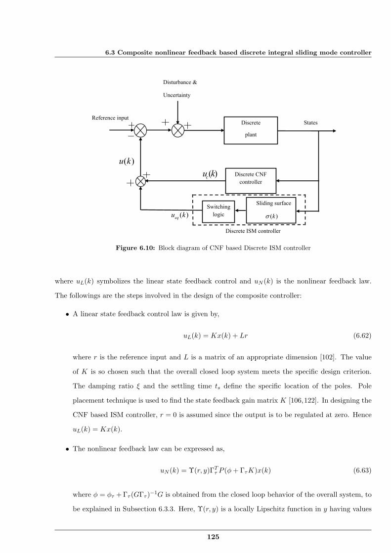
6.3 Composite nonlinear feedback based discrete integral sliding mode controller
Discrete
plant
Discrete CNF
controller
Sliding surface
( )k
Switching
logic
Reference input
Disturbance &
Uncertainty
Discrete ISM controller
States
( )cu k
( )equ k
( )u k
Figure 6.10: Block diagram of CNF based Discrete ISM controller
where uL(k) symbolizes the linear state feedback control and uN (k) is the nonlinear feedback law.
The followings are the steps involved in the design of the composite controller:
• A linear state feedback control law is given by,
uL(k) = Kx(k) + Lr (6.62)
where r is the reference input and L is a matrix of an appropriate dimension [102]. The value
of K is so chosen such that the overall closed loop system meets the specific design criterion.
The damping ratio ξ and the settling time ts define the specific location of the poles. Pole
placement technique is used to find the state feedback gain matrix K [106,122]. In designing the
CNF based ISM controller, r = 0 is assumed since the output is to be regulated at zero. Hence
uL(k) = Kx(k).
• The nonlinear feedback law can be expressed as,
uN (k) = Υ(r, y)ΓTτ P (ϕ+ ΓτK)x(k) (6.63)
where ϕ = ϕτ + Γτ (GΓτ )−1G is obtained from the closed loop behavior of the overall system, to
be explained in Subsection 6.3.3. Here, Υ(r, y) is a locally Lipschitz function in y having values
125
6. Nonlinear Sliding Surface based Adaptive Sliding Mode Controller
from zero to negative. Furthermore, Υ(r, y) is used to change the damping ratio of the closed
loop system as the output approaches the reference input. Then P > 0 is the solution of the
following Lyapunov equation,
P = (ϕ+ ΓτK)TP (ϕ+ ΓτK) +R (6.64)
where R is a positive definite matrix.
• The linear and nonlinear feedback control laws expressed in (6.62) and (6.63) can be combined
to get the overall expression for the CNF controller as
uc(k) = Kx(k) + Υ(r, y)ΓTτ P (ϕ+ ΓτK)x(k) (6.65)
Using (6.53), (6.56) and (6.65), the overall discrete CNF-ISM control law can be expressed as
u(k) = Kx(k) + Υ(r, y)ΓTτ P (ϕ+ ΓτK)x(k) + (GΓτ )−1(Gx(0) −GΓτ d(k) − h(k)) (6.66)
6.3.3 Closed loop behavior and stability of the overall system
Using (6.49), the discrete state equation can be written as,
x(k + 1) = ϕτx(k) + Γτu(k) + Γτd(k) (6.67)
where u(k) = uc(k) + ueq(k) is the overall control input.
Using (6.53) and (6.67) yields,
x(k + 1) = ϕτx(k) + Γτ (uc(k) + ueq(k)) + Γτd(k) (6.68)
Using (6.56), (6.68) can be expressed as,
x(k + 1) = ϕτx(k) + Γτuc(k) + Γτ (d(k) − d(k))
+Γτ (GΓτ )−1Gx(0) − Γτ (GΓτ )−1h(k) (6.69)
126
6.3 Composite nonlinear feedback based discrete integral sliding mode controller
Using (6.50) and (6.65), (6.69) can be expressed as,
x(k + 1) = ϕτx(k) + Γτ (Kx(k) + Υ(r, y)ΓTτ P (ϕ+ ΓτK)x(k))
+Γτ (d(k) − d(k)) − Γτ (GΓτ )−1(σ(k) −Gx(k)) (6.70)
Using (6.60), σ(k) is obtained as,
σ(k) = GΓτ (d(k − 1) − d(k − 2)) (6.71)
Using (6.71), (6.70) can be obtained as,
x(k + 1) = ϕτx(k) + Γτ (Kx(k) + Υ(r, y)ΓTτ P (ϕ+ ΓτK)x(k))
+Γτ (d(k) − 2d(k − 1) + d(k − 2)) + Γτ (GΓτ )−1Gx(k) (6.72)
Remark 6.2. The proposed method uses the bound of the variation/difference of the disturbance,
d(k−1)−d(k−2) where k = 0, 1, 2, , , , . It is clear that disturbance decreases as the sampling frequency
increases. The magnitude of the ultimate bound of the state x(k) can be made very small if the
disturbance d(k) varies slowly or the sampling period is set very short and hence more accurate results
can be obtained.
Remark 6.3. Here Υ(r, y) is a nonlinear function which has values varying from zero to a high
negative value. Initially it is assumed that Υ(r, y) = 0, which later assumes a high negative value.
When Υ(r, y) = 0 is considered, (6.72) becomes,
x(k + 1) = (ϕτ + Γτ (GΓτ )−1G+ ΓτK)x(k) + Γτ [d(k) − 2d(k − 1) + d(k − 2)] (6.73)
Thus the boundary layer thickness is given by [7],
O(τ3) = Γτ [d(k) − 2d(k − 1) + d(k − 2)] (6.74)
From (6.73 - 6.74) it can be observed that x(k) will stay in the neighborhood of the reference
state within a boundary of O(τ3) [7]. It is noteworthy that by using the discrete integral sliding mode
controller, disturbance can be better compensated with smaller steady state boundary and higher
accuracy.
Let us assume that d(k) is bounded as given by −M ≤ Γτ [d(k) − 2d(k − 1) + d(k − 2)] = w(k) ≤ M
127
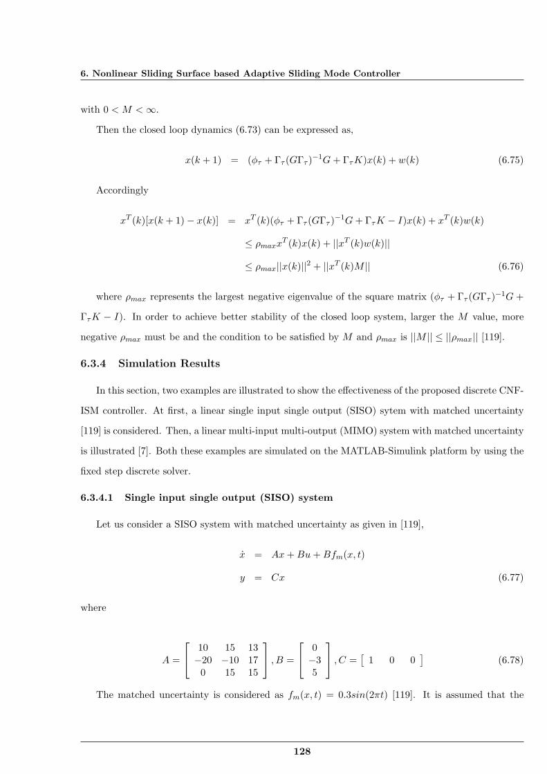
6. Nonlinear Sliding Surface based Adaptive Sliding Mode Controller
with 0 < M <∞.
Then the closed loop dynamics (6.73) can be expressed as,
x(k + 1) = (ϕτ + Γτ (GΓτ )−1G+ ΓτK)x(k) + w(k) (6.75)
Accordingly
xT (k)[x(k + 1) − x(k)] = xT (k)(ϕτ + Γτ (GΓτ )−1G+ ΓτK − I)x(k) + xT (k)w(k)
≤ ρmaxxT (k)x(k) + ||xT (k)w(k)||
≤ ρmax||x(k)||2 + ||xT (k)M || (6.76)
where ρmax represents the largest negative eigenvalue of the square matrix (ϕτ + Γτ (GΓτ )−1G +
ΓτK − I). In order to achieve better stability of the closed loop system, larger the M value, more
negative ρmax must be and the condition to be satisfied by M and ρmax is ||M || ≤ ||ρmax|| [119].
6.3.4 Simulation Results
In this section, two examples are illustrated to show the effectiveness of the proposed discrete CNF-
ISM controller. At first, a linear single input single output (SISO) sytem with matched uncertainty
[119] is considered. Then, a linear multi-input multi-output (MIMO) system with matched uncertainty
is illustrated [7]. Both these examples are simulated on the MATLAB-Simulink platform by using the
fixed step discrete solver.
6.3.4.1 Single input single output (SISO) system
Let us consider a SISO system with matched uncertainty as given in [119],
x = Ax+Bu+Bfm(x, t)
y = Cx (6.77)
where
A =
10 15 13−20 −10 170 15 15
, B =
0−35
, C =[
1 0 0]
(6.78)
The matched uncertainty is considered as fm(x, t) = 0.3sin(2πt) [119]. It is assumed that the
128
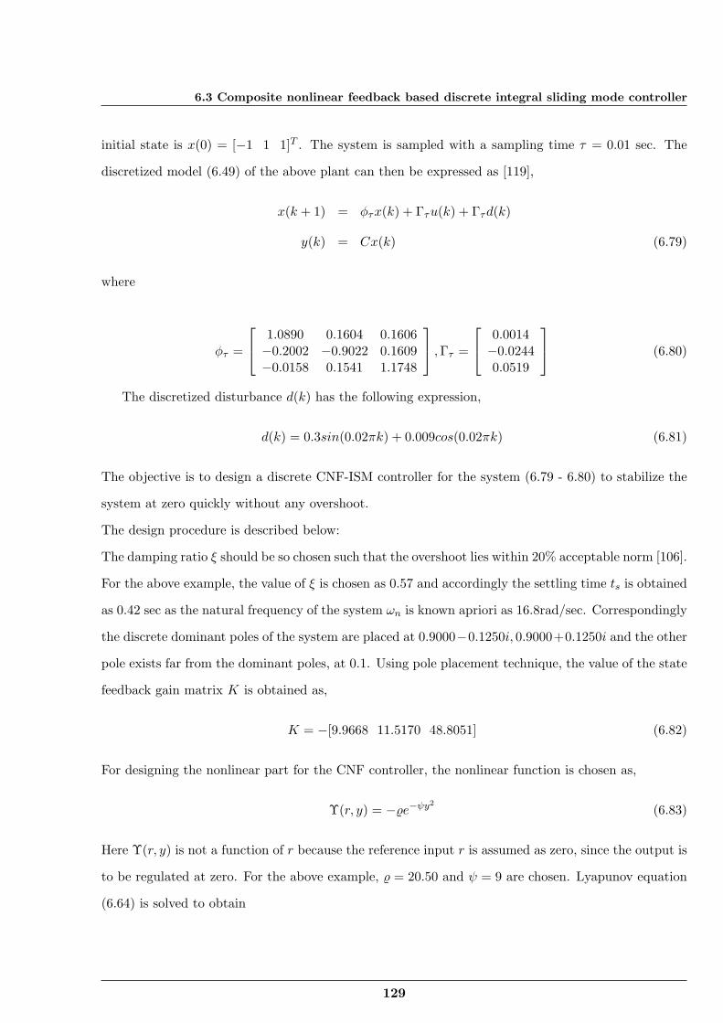
6.3 Composite nonlinear feedback based discrete integral sliding mode controller
initial state is x(0) = [−1 1 1]T . The system is sampled with a sampling time τ = 0.01 sec. The
discretized model (6.49) of the above plant can then be expressed as [119],
x(k + 1) = ϕτx(k) + Γτu(k) + Γτd(k)
y(k) = Cx(k) (6.79)
where
ϕτ =
1.0890 0.1604 0.1606−0.2002 −0.9022 0.1609−0.0158 0.1541 1.1748
,Γτ =
0.0014−0.02440.0519
(6.80)
The discretized disturbance d(k) has the following expression,
d(k) = 0.3sin(0.02πk) + 0.009cos(0.02πk) (6.81)
The objective is to design a discrete CNF-ISM controller for the system (6.79 - 6.80) to stabilize the
system at zero quickly without any overshoot.
The design procedure is described below:
The damping ratio ξ should be so chosen such that the overshoot lies within 20% acceptable norm [106].
For the above example, the value of ξ is chosen as 0.57 and accordingly the settling time ts is obtained
as 0.42 sec as the natural frequency of the system ωn is known apriori as 16.8rad/sec. Correspondingly
the discrete dominant poles of the system are placed at 0.9000−0.1250i, 0.9000+0.1250i and the other
pole exists far from the dominant poles, at 0.1. Using pole placement technique, the value of the state
feedback gain matrix K is obtained as,
K = −[9.9668 11.5170 48.8051] (6.82)
For designing the nonlinear part for the CNF controller, the nonlinear function is chosen as,
Υ(r, y) = −ϱe−ψy2 (6.83)
Here Υ(r, y) is not a function of r because the reference input r is assumed as zero, since the output is
to be regulated at zero. For the above example, ϱ = 20.50 and ψ = 9 are chosen. Lyapunov equation
(6.64) is solved to obtain
129
6. Nonlinear Sliding Surface based Adaptive Sliding Mode Controller
P =
426.0891 116.4046 93.5674116.4046 129.6438 90.865493.5674 90.8654 79.2154
using R =
10.00 0.000 0.0000.000 10.00 0.0000.000 0.000 10.00
(6.84)
So, the composite nonlinear feedback (CNF) controller (6.65) designed for the above system yields
the following control law,
uc(k) = −[9.9668 11.5170 48.8051]x(k) + Υ(r, y)[1.8311 1.0123 0.8646]x(k) (6.85)
For designing the equivalent control of the integral sliding mode controller (i.e.ueq(k)), G is chosen
as [20],
G = (ΓTτ Γτ )−1ΓTτ (6.86)
Using (6.80) and (6.86) yields,
G = [0.4254 − 7.4143 15.7706] (6.87)
Using (6.80) and (6.87), the equivalent control law (6.56) is found as,
ueq(k) = −d(k) − h(k) + [0.4254 − 7.4143 15.7706]x(0) (6.88)
The overall control law of the proposed discrete CNF-ISM controller (6.66) can be expressed as,
u(k) = −[9.9668 11.5170 48.8051]x(k) + Υ(r, y)[1.8311 1.0123 0.8646]x(k)
−d(k) − h(k) + [0.4254 − 7.4143 15.7706]x(0) (6.89)
Fig. 6.11 shows the state x1 obtained by using the proposed discrete CNF-ISM control scheme for the
SISO system given by (6.79 - 6.80) and is compared with the results obtained by using the discrete ISM
controller (6.57). It is noticed that the proposed discrete CNF-ISM control scheme achieves superior
performance having zero overshoot and lower settling time. However, the rise time is almost the same
in both the cases.
Figs. 6.12 - 6.13 show the states x2 and x3 obtained by using the proposed discrete CNF-ISM controller
as well as the discrete ISM controller (6.57). It is observed that with the proposed discrete CNF-ISM
controller, the closed loop system settles more quickly with no overshoot as compared against the
discrete ISM controller.
130
6.3 Composite nonlinear feedback based discrete integral sliding mode controller
0 0.1 0.2 0.3 0.4 0.5 0.6 0.7 0.8 0.9 1−1
−0.8
−0.6
−0.4
−0.2
0
0.2
0.4
Time (sec)
x1
proposed discrete CNF−ISM controllerdiscrete ISM controller
Figure 6.11: System state x1 ; solid line with proposed discrete CNF-ISM controller and broken line withdiscrete ISM controller
0 0.1 0.2 0.3 0.4 0.5 0.6 0.7 0.8 0.9 1−0.5
0
0.5
1
1.5
2
2.5
Time (sec)
x2
proposed discrete CNF−ISM controllerdiscrete ISM controller
Figure 6.12: System state x2 ; solid line with proposed discrete CNF-ISM controller and broken line withdiscrete ISM Controller
Fig. 6.14 compares the the control inputs obtained for the proposed discrete CNF-ISM controller
against the discrete ISM controller (6.57). The energy norm of the input for the proposed discrete
CNF-ISM controller is 43.65 and that of the discrete ISM controller is 43.44. The proposed discrete
CNF-ISM controller uses 0.5% more energy in comparison to the discrete ISM controller.
131
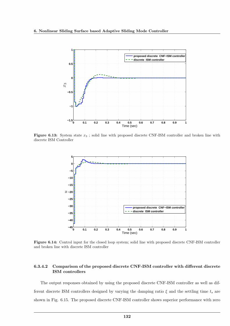
6. Nonlinear Sliding Surface based Adaptive Sliding Mode Controller
0 0.1 0.2 0.3 0.4 0.5 0.6 0.7 0.8 0.9 1−1.5
−1
−0.5
0
0.5
1
Time (sec)
x3
proposed discrete CNF−ISM controllerdiscrete ISM controller
Figure 6.13: System state x3 ; solid line with proposed discrete CNF-ISM controller and broken line withdiscrete ISM Controller
0 0.1 0.2 0.3 0.4 0.5 0.6 0.7 0.8 0.9 1−45
−40
−35
−30
−25
−20
−15
−10
−5
0
5
Time (sec)
u
proposed discrete CNF−ISM controllerdiscrete ISM controller
Figure 6.14: Control input for the closed loop system; solid line with proposed discrete CNF-ISM controllerand broken line with discrete ISM controller
6.3.4.2 Comparison of the proposed discrete CNF-ISM controller with different discreteISM controllers
The output responses obtained by using the proposed discrete CNF-ISM controller as well as dif-
ferent discrete ISM controllers designed by varying the damping ratio ξ and the settling time ts are
shown in Fig. 6.15. The proposed discrete CNF-ISM controller shows superior performance with zero
132
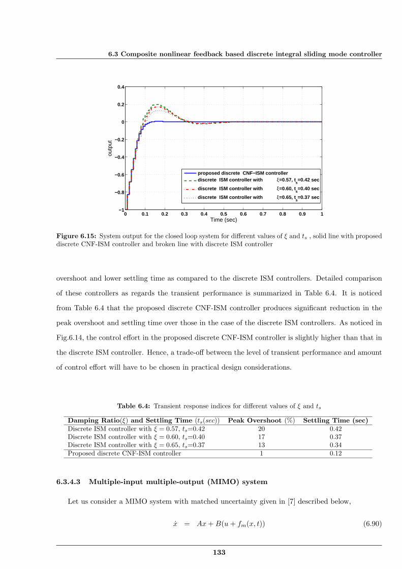
6.3 Composite nonlinear feedback based discrete integral sliding mode controller
0 0.1 0.2 0.3 0.4 0.5 0.6 0.7 0.8 0.9 1−1
−0.8
−0.6
−0.4
−0.2
0
0.2
0.4
Time (sec)
outp
ut
proposed discrete CNF−ISM controllerdiscrete ISM controller with ξ=0.57, t
s=0.42 sec
discrete ISM controller with ξ=0.60, ts=0.40 sec
discrete ISM controller with ξ=0.65, ts=0.37 sec
Figure 6.15: System output for the closed loop system for different values of ξ and ts , solid line with proposeddiscrete CNF-ISM controller and broken line with discrete ISM controller
overshoot and lower settling time as compared to the discrete ISM controllers. Detailed comparison
of these controllers as regards the transient performance is summarized in Table 6.4. It is noticed
from Table 6.4 that the proposed discrete CNF-ISM controller produces significant reduction in the
peak overshoot and settling time over those in the case of the discrete ISM controllers. As noticed in
Fig.6.14, the control effort in the proposed discrete CNF-ISM controller is slightly higher than that in
the discrete ISM controller. Hence, a trade-off between the level of transient performance and amount
of control effort will have to be chosen in practical design considerations.
Table 6.4: Transient response indices for different values of ξ and ts
Damping Ratio(ξ) and Settling Time (ts(sec)) Peak Overshoot (%) Settling Time (sec)Discrete ISM controller with ξ = 0.57, ts=0.42 20 0.42Discrete ISM controller with ξ = 0.60, ts=0.40 17 0.37Discrete ISM controller with ξ = 0.65, ts=0.37 13 0.34Proposed discrete CNF-ISM controller 1 0.12
6.3.4.3 Multiple-input multiple-output (MIMO) system
Let us consider a MIMO system with matched uncertainty given in [7] described below,
x = Ax+B(u+ fm(x, t)) (6.90)
133
6. Nonlinear Sliding Surface based Adaptive Sliding Mode Controller
where
A =
1 −2 3−4 5 −67 −8 9
, B =
1 −2−3 45 6
, fm(x, t) =[
0.3sin(4πt)0.3cos(4πt)
](6.91)
The initial state is at x(0) = [1 1 − 1]T . The system is sampled at a time interval of τ = 0.001
sec. A suitable nonlinear function Υ(r, y) is used that has a very low value at the initial stage and has
a relatively higher value when the system approaches its final state [109]. Here the chosen nonlinear
function is,
Υ(r, y) = −57.3871e−8y2 (6.92)
For a system, overshoot less than 20% is acceptable [102, 106] and hence the poles are selected by
choosing the damping ratio ξ = 0.7 and accordingly the settling time ts is 0.5 sec. Accordingly, the
dominant poles are found as 0.9510+0.1520i and 0.9510-0.1520i while the other pole is placed far away
at 0.1 [123]. Using pole placement technique, the state feedback gain matrix can be calculated as,
K =[
769.1649 42.8508 126.9456129.9735 312.7895 108.7556
](6.93)
In order to find the the CNF control law from (6.65), Lyapunov equation (6.64)is solved to obtain
P =
397.5233 167.4345 20.2155167.4345 70.7267 8.009720.2155 8.0097 4.1436
using R =
0.100 0.000 0.0000.000 0.100 0.0000.000 0.000 0.100
(6.94)
The Matrix G is chosen as [7],
G =[
0.2621 −0.3108 −0.03853.4268 2.4432 1.1787
](6.95)
Fig.6.16 shows the state x1 obtained by using the proposed discrete CNF-ISM controller and is
compared with that obtained by using the discrete ISM control scheme by Abidi et al. [7]. It shows
clearly that both the rise time and the settling time can be minimized simultaneously by using the
proposed discrete CNF-ISM controller. Transient performance indices evaluated by using both these
controllers are compared in Table 6.5. It is noted from Table 6.5 that the proposed controller shows
superior transient performance by reducing the rise time and settling time by about 63% from those
134
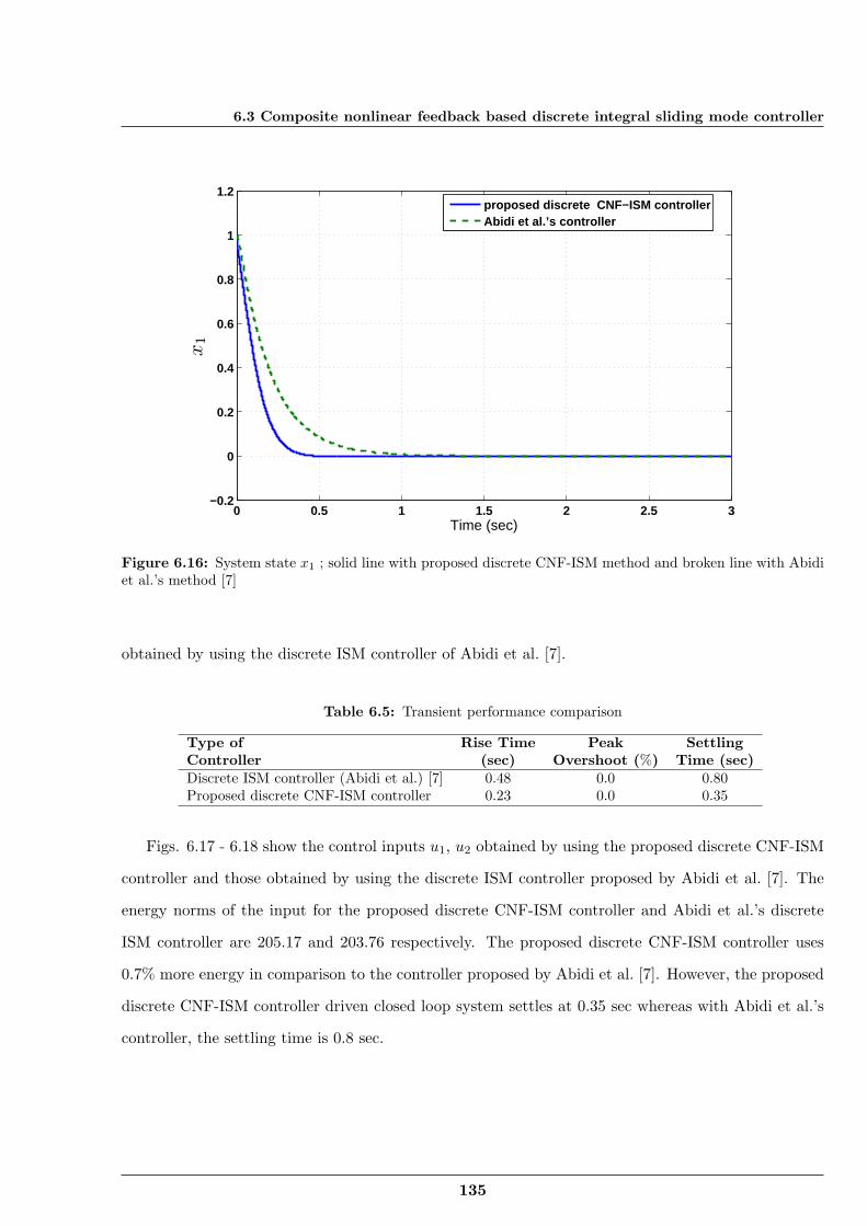
6.3 Composite nonlinear feedback based discrete integral sliding mode controller
0 0.5 1 1.5 2 2.5 3−0.2
0
0.2
0.4
0.6
0.8
1
1.2
Time (sec)
x1
proposed discrete CNF−ISM controllerAbidi et al.’s controller
Figure 6.16: System state x1 ; solid line with proposed discrete CNF-ISM method and broken line with Abidiet al.’s method [7]
obtained by using the discrete ISM controller of Abidi et al. [7].
Table 6.5: Transient performance comparison
Type of Rise Time Peak SettlingController (sec) Overshoot (%) Time (sec)Discrete ISM controller (Abidi et al.) [7] 0.48 0.0 0.80Proposed discrete CNF-ISM controller 0.23 0.0 0.35
Figs. 6.17 - 6.18 show the control inputs u1, u2 obtained by using the proposed discrete CNF-ISM
controller and those obtained by using the discrete ISM controller proposed by Abidi et al. [7]. The
energy norms of the input for the proposed discrete CNF-ISM controller and Abidi et al.’s discrete
ISM controller are 205.17 and 203.76 respectively. The proposed discrete CNF-ISM controller uses
0.7% more energy in comparison to the controller proposed by Abidi et al. [7]. However, the proposed
discrete CNF-ISM controller driven closed loop system settles at 0.35 sec whereas with Abidi et al.’s
controller, the settling time is 0.8 sec.
135
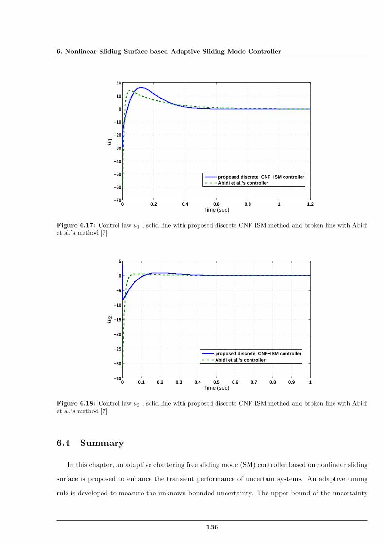
6. Nonlinear Sliding Surface based Adaptive Sliding Mode Controller
0 0.2 0.4 0.6 0.8 1 1.2−70
−60
−50
−40
−30
−20
−10
0
10
20
Time (sec)
u1
proposed discrete CNF−ISM controllerAbidi et al.’s controller
Figure 6.17: Control law u1 ; solid line with proposed discrete CNF-ISM method and broken line with Abidiet al.’s method [7]
0 0.1 0.2 0.3 0.4 0.5 0.6 0.7 0.8 0.9 1−35
−30
−25
−20
−15
−10
−5
0
5
Time (sec)
u2
proposed discrete CNF−ISM controllerAbidi et al.’s controller
Figure 6.18: Control law u2 ; solid line with proposed discrete CNF-ISM method and broken line with Abidiet al.’s method [7]
6.4 Summary
In this chapter, an adaptive chattering free sliding mode (SM) controller based on nonlinear sliding
surface is proposed to enhance the transient performance of uncertain systems. An adaptive tuning
rule is developed to measure the unknown bounded uncertainty. The upper bound of the uncertainty
136
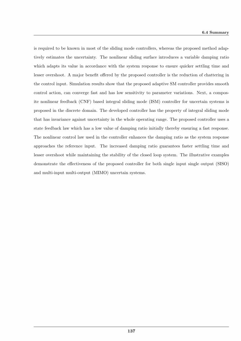
6.4 Summary
is required to be known in most of the sliding mode controllers, whereas the proposed method adap-
tively estimates the uncertainty. The nonlinear sliding surface introduces a variable damping ratio
which adapts its value in accordance with the system response to ensure quicker settling time and
lesser overshoot. A major benefit offered by the proposed controller is the reduction of chattering in
the control input. Simulation results show that the proposed adaptive SM controller provides smooth
control action, can converge fast and has low sensitivity to parameter variations. Next, a compos-
ite nonlinear feedback (CNF) based integral sliding mode (ISM) controller for uncertain systems is
proposed in the discrete domain. The developed controller has the property of integral sliding mode
that has invariance against uncertainty in the whole operating range. The proposed controller uses a
state feedback law which has a low value of damping ratio initially thereby ensuring a fast response.
The nonlinear control law used in the controller enhances the damping ratio as the system response
approaches the reference input. The increased damping ratio guarantees faster settling time and
lesser overshoot while maintaining the stability of the closed loop system. The illustrative examples
demonstrate the effectiveness of the proposed controller for both single input single output (SISO)
and multi-input multi-output (MIMO) uncertain systems.
137
7Conclusions and Scope for Future
Work
Contents
7.1 Conclusions . . . . . . . . . . . . . . . . . . . . . . . . . . . . . . . . . . . . . 139
7.2 Scope for future work . . . . . . . . . . . . . . . . . . . . . . . . . . . . . . . 140
138
7.1 Conclusions
7.1 Conclusions
This thesis attempts to design sliding mode controllers for uncertain systems having both matched
and mismatched types of uncertainty. In conventional first order sliding mode controllers, chattering in
the control input is the major disadvantage. Of late, second and higher order sliding mode controllers
have evolved promising better chattering mitigation. This thesis attempts to design chattering free
sliding mode (SM) controllers to overcome the shortcomings of conventional first order sliding mode
controllers. The basic philosophy of the proposed control scheme is that instead of the normal con-
trol input, its time derivative is used for designing the controller. The discontinuous sign function
is contained in the derivative control and the actual control is obtained by integrating the discontin-
uous sign function and hence it is continuous and smooth. This strategy is the core idea which is
followed in this thesis to develop sliding mode controllers of different types. Another limitation of the
conventional sliding mode controllers is the design prerequisite of knowing the upper bound of the
system uncertainty apriori which is practically difficult to realize. The proposed controller attempts
to overcome this difficulty by using an adaptive gain tuning methodology.
An adaptive integral sliding mode controller using chattering free sliding mode technique is proposed
in this thesis. Reaching phase is totally eliminated in the integral sliding mode and hence the system
becomes invariant towards the matching uncertainty right from the beginning. Application of the
proposed controller to both stabilization and tracking problems of single input single output (SISO)
system demonstrates the efficacy of the proposed control strategy.
An adaptive chattering free sliding mode control scheme is proposed for a class of dynamic systems with
matched and mismatched perturbations. The controller is used to stabilize the twin rotor MIMO sys-
tem (TRMS) in significant cross-couplings to reach a desired position and accurately track a specified
trajectory. The TRMS model is divided into a horizontal and a vertical subsystem. The cross-coupling
existing between the two subsystems is considered as the system uncertainty. The major advantage
offered by this adaptive sliding mode controller is that advance knowledge about the upper bound of
the system uncertainty is not a necessary requirement and the control input is smooth. The problem
of controlling of a vertical take-off and landing (VTOL) aircraft system affected by both types of
uncertainties, matched and mismatched, is also addressed by applying the proposed control scheme.
A proportional plus integral sliding surface is used in the proposed control technique. An adaptive
gain tuning mechanism is used to ensure that the switching gain is not overestimated with respect to
139
7. Conclusions and Scope for Future Work
the actual unknown value of the uncertainty.
Experimental studies conducted on the laboratory set-up of 1 degree of freedom VTOL system validate
the efficacy of the proposed controller.
An adaptive terminal sliding mode (TSM) controller is proposed where the nonsingular terminal slid-
ing manifold guarantees fast and finite time convergence. The proposed adaptive TSM controller is
successfully applied for stabilization of a triple integrator system affected by uncertainty. Trajectory
tracking of a two-link robotic manipulator which is a nonlinear system with mismatched uncertainty
is considered which demonstrates the efficiency of the proposed control strategy.
A nonlinear sliding surface based chattering free adaptive sliding mode controller is proposed to im-
prove the transient performance of an uncertain system. The basic philosophy of the proposed scheme
is that using a nonlinear sliding surface, the damping ratio of a system can be changed from its initial
low value to a final high value. The initial low value of damping ratio results in a quick response
and the later high damping avoids overshoot. To improve the transient performance in discrete time
uncertain systems, an integral sliding mode is used with composite nonlinear feedback (CNF).
The control strategies developed in this thesis using the chattering free adaptive sliding mode show
robust performance even in presence of matched and mismatched uncertainties. The controllers de-
veloped ensure high transient performance while preserving the robustness property of conventional
sliding mode controllers but successfully overcoming their inherent chattering disadvantage. As such,
the proposed control strategies promise high application potential in many important fields like elec-
tric drives, robotics, power electronics, servo applications and aerospace where performance needs to
be guaranteed consistently despite being challenged by an uncertain environment.
7.2 Scope for future work
Future possible directions of research based on the design methods developed in this thesis are
outlined below:
• A natural extension of this work may be to design discrete sliding mode algorithms with adap-
tive techniques which will enhance the flexibility in implementation. Now-a-days, a large class
of continuous systems are controlled by digital signal processors (DSPs) and high end micro
controllers. Hence discrete SM controller will be easier and effective from implementation point
of view.
140
7.2 Scope for future work
• Another possible extension of this work may be the incorporation of an optimal sliding mode
controller to optimize the control effort.
• Nonlinear sliding surface based adaptive sliding mode controller may be extended to improve
the transient performance of general references, such as sinusoidal and other periodic signals.
• The proposed design method may be extended by using intelligent controllers based on fuzzy
logic and neural network to incorporate flexibility and intelligence.
• The extension of these techniques with constraints on system states is also an avenue worth
exploring.
• The high performance requirement of many practical applications like electric drives, electro-
pneumatics, power system stabilizers and robotics may be addressed by using the proposed
techniques.
141

AAppendix
Contents
A.1 Modeling of 1 DOF VTOL Aircraft System . . . . . . . . . . . . . . . . . . 143
142
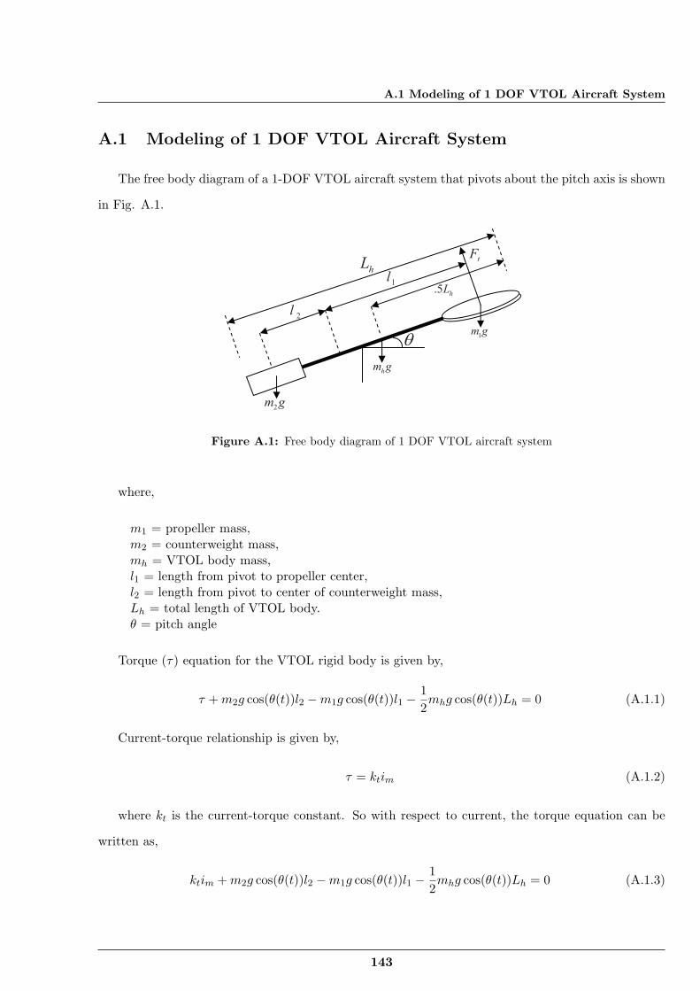
A.1 Modeling of 1 DOF VTOL Aircraft System
A.1 Modeling of 1 DOF VTOL Aircraft System
The free body diagram of a 1-DOF VTOL aircraft system that pivots about the pitch axis is shown
in Fig. A.1.
tF
2m g
hm g
1m g
.5 hL1l
2l
hL
Figure A.1: Free body diagram of 1 DOF VTOL aircraft system
where,
m1 = propeller mass,m2 = counterweight mass,mh = VTOL body mass,l1 = length from pivot to propeller center,l2 = length from pivot to center of counterweight mass,Lh = total length of VTOL body.θ = pitch angle
Torque (τ) equation for the VTOL rigid body is given by,
τ +m2g cos(θ(t))l2 −m1g cos(θ(t))l1 −12mhg cos(θ(t))Lh = 0 (A.1.1)
Current-torque relationship is given by,
τ = ktim (A.1.2)
where kt is the current-torque constant. So with respect to current, the torque equation can be
written as,
ktim +m2g cos(θ(t))l2 −m1g cos(θ(t))l1 −12mhg cos(θ(t))Lh = 0 (A.1.3)
143
A. Appendix
In equilibrium condition i.e. when θ = 0, im becomes ieq and torque equation becomes,
ktieq +m2gl2 −m1gl1 −12mhgLh = 0 (A.1.4)
Angular (pitch) motion with respect to thrust torque τ is given by,
jθ(t) + bv θ(t) + kθ(t) = τ = ktim (A.1.5)
Here bv is the viscous damping, k is the stiffness and j is the equivalent moment of inertia acting
about the pitch axis, which is given by,
j =n∑i=1
mir2i (A.1.6)
where for object i, mi is its mass and ri is the perpendicular distance between the axis of rotation
and the object. So the transfer function for the VTOL system can be obtained as,
G(s) =θ(s)Im(s)
=ktj
s2 + bvsj + k
j
(A.1.7)
By comparing the denominator of (A.1.7) with the characteristic equation of a second order system,
s2 + 2ζωns+ ω2n (A.1.8)
the damping ratio ζ and natural frequency ωn can be easily found out.
Voltage-current equation for the VTOL motor is given by,
vm(t) = Rmim(t) + Lmim(t) (A.1.9)
where Rm is the motor resistance and Lm is the motor inductance. So the transfer function of the
VTOL motor is obtained as,
Im(s)Vm(s)
=1
Rm + Lms(A.1.10)
The output-input relationship of the VTOL needs to be obtained as position-voltage relationship
144
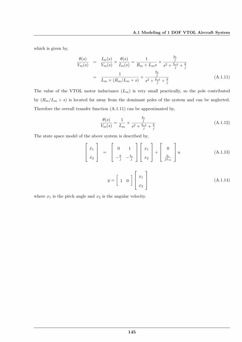
A.1 Modeling of 1 DOF VTOL Aircraft System
which is given by,
θ(s)Vm(s)
=Im(s)Vm(s)
× θ(s)Im(s)
=1
Rm + Lms×
ktj
s2 + bvsj + k
j
=1
Lm × (Rm/Lm + s)×
ktj
s2 + bvsj + k
j
(A.1.11)
The value of the VTOL motor inductance (Lm) is very small practically, so the pole contributed
by (Rm/Lm + s) is located far away from the dominant poles of the system and can be neglected.
Therefore the overall transfer function (A.1.11) can be approximated by,
θ(s)Vm(s)
=1Lm
×ktj
s2 + bvsj + k
j
(A.1.12)
The state space model of the above system is described by, x1
x2
=
0 1
−kj − bv
j
x1
x2
+
0
ktjLm
u (A.1.13)
y =[
1 0
] x1
x2
(A.1.14)
where x1 is the pitch angle and x2 is the angular velocity.
145
References
[1] C. W. Tao, J. S. Taur, and Y. C. Chen, “Design of a parallel distributed fuzzy lqrc ontroller for the twin
rotor multi-inputmulti-output system,” Fuzzy Sets and Systems, vol. 161, pp. 2081–2103, 2010.
[2] Y. J. Huang, T. C. Kuo, and H. K. Way, “Robust vertical takeoff and landing aircraft control via integral
sliding mode,” IEE Procedings Control Theory Application, vol. 150, (4), pp. 383–388, 2003.
[3] C. C. Wen and C. C. Cheng, “Design of sliding surface for mismatched uncertain systems to achieve
asymptotical stability,” Journal of the Franklin Institute, vol. 345, pp. 926–941, 2008.
[4] M. Defoort, F. Nollet, T. Floquet, and W. Perruquetti, “A third-order sliding-mode controller for a stepper
motor,” IEEE Transactions on Industrial Electronics, vol. 56, (9), pp. 3337 – 3346, 2009.
[5] Y. Feng, X. Yu, and Z. Man, “Non-singular terminal sliding mode control of rigid manipulators,” Auto-
matica, vol. 38, pp. 2159 –2167, 2002.
[6] D. Fulwani, B. Bandyopadhyay, and L. Fridman, “Non-linear sliding surface: towards high performance
robust control,” IET Control Theory and Applications, vol. 6(2), pp. 235–242, 2012.
[7] K. Abidi, J.-X. Xu, and Y. Xinghuo, “On the discrete-time integral sliding-mode control,” IEEE Trans-
actions on Automatic Control, vol. 52, (4), pp. 709–715, 2007.
[8] C. W. Tao, J. S. Taur, Y. H. Chang, and C. W. Chang, “A novel fuzzy-sliding and fuzzy-integral-sliding
controller for the twin-rotor multi-input multi-output system,” IEEE Transactions on Fuzzy Systems, vol.
18, (5), pp. 893–905, 2010.
[9] K. J. Astrom and B. Wittenmark, Computer-Controlled Systems, Theory and Design. Prentice-Hall,
1990.
[10] E. F. Camacho and C. Bordons, Model Predictive Control. Springer, 2004.
[11] F. Ikhouane and M. Krstic, “Robustness of the tuning functions adaptive backstepping design for linear
systems,” IEEE Transactions on Automatic Control, vol. 43(3), pp. 431–437, 1998.
[12] W. Perruquetti and J. P. Barbot, Sliding mode control in Engineering, Automation and Control Series.
Marcel Dekker Inc., New York (USA), 2002.
146
References
[13] H. K. Khalil, Nonlinear Systems, Third Edition. Prentice Hall, 2002.
[14] S. V. Emelyanov, “Variable structure control systems,” Nauka, vol. 35, pp. 120–125, 1967.
[15] V. I. Utkin, “Variable structure systems with sliding modes,” IEEE Transactions on Automatic Control,
vol. 22 (2), pp. 212–222, 1977.
[16] J. Y. Hang, W. Gao, and J. C. Hung, “Variable structure control: A survey,” IEEE Transactions on
Industrial Electronics, vol. 40, (1), pp. 2 – 22, 1993.
[17] K. K. Young, Variable Structure Control for Robotics and Aerospace Systems. Elsevier, Amsterdam, The
Netherlands, 1993.
[18] U. Itkis, Control systems of variable structure. Wiley, New York, 1976.
[19] V. I. Utkin and J. Shi, “Integral sliding mode in systems operating under uncertainty conditions,” in
Proceedings of the 35th IEEE conference on decision and control, pp. 4591-4596, 1996.
[20] F. Castanos and L. Fridman, “Analysis and design of integral sliding manifolds for systems with unmatched
perturbations,” IEEE Transactions on Automatic Control, vol. 51, (5), pp. 853–858, 2006.
[21] V. I. Utkin, J. Guldner, and J. Shi, Sliding Mode Control in Electromechanical Systems. Taylor & Francis,
London, UK, 1999.
[22] C. Edwards and S. K. Spurgeon, Sliding mode control: theory and applications. Taylor & Francis, London,
U.K., 1998.
[23] J.-J. Slotine and W. Li, Applied nonlinear control. Prentice Hall, Englewood Cliffs, NJ, USA, 1991.
[24] A. Levant, “Sliding order and sliding accuracy in sliding mode control,” International Journal of Control,
vol. 58, (6), pp. 1247–1263, 1993.
[25] ——, “Higher-order sliding modes, differentiation and output-feedback control,” International Journal of
Control, vol. 76, (9/10), pp. 924–941, 2003.
[26] ——, “Universal single-input single-output (SISO) sliding-mode controllers with finite-time convergence,”
IEEE Transactions on Automatic Control, vol. 46, (1), pp. 1447–1451, 2001.
[27] G. Bartolini, A. Ferrara, and E. Usai, “Chattering avoidance by second-order sliding mode control,” IEEE
Transactions on Automatic Control, vol. 43, (2), pp. 241–246, 1998.
[28] G. Bartolini, A. Ferrara, E. Usai, and V. I. Utkin, “On multi-input chattering-free second-order sliding
mode control,” IEEE Transactions on Automatic Control, vol. 45(8), pp. 1711–1717, 2000.
[29] G. Bartolini, A. Ferrara, and E. Punta, “Multi-input second-order sliding-mode hybrid control of con-
strained manipulators,” Dynamics and Control, vol. 10, (3), pp. 277–296, 2000.
147
References
[30] V. I. Utkin, Sliding Modes in Control and Optimization. Springer, Berlin, 1992.
[31] C. W. Tao, M.-L. Chan, and T.-T. Lee, “Adaptive fuzzy sliding mode controller for linear systems with
mismatched time-varying uncertainties,” IEEE Transactions on Systems, Man, and Cybernetics Part B:
Cybernetics, vol. 33, (2), pp. 283–294, 2003.
[32] H. H. Choi, “An explicit formula of linear sliding surfaces for a class of uncertain dynamic systems with
mismatched uncertainties,” Automatica, vol. 34, (8), pp. 1015–1020, 1998.
[33] ——, “An lmi-based switching surface design method for a class of mismatched uncertain systems,” IEEE
Transactions on Automatic Control, vol. 48, (9), pp. 1634–1638, 2003.
[34] Y.-W. Tsai, K.-K. Shyu, and K.-C. Chang, “Decentralized variable structure control for mismatched
uncertain large-scale systems: a new approach,” System and Control Letters, vol. 43, (2), pp. 117–125,
2001.
[35] K.-K. Shyu, Y.-W. Tsai, and C.-K. Lai, “A dynamic output feedback controllers for mismatched uncertain
variable structure systems,” Automatica, vol. 37, (5), pp. 775–779, 2001.
[36] W.-J. Cao and J.-X. Xu, “Nonlinear integral-type sliding surface for both matched and unmatched un-
certain systems,” IEEE Transactions on Automatic Control, vol. 49, (8), pp. 1355–1360, 2004.
[37] C.-H. Chou and C.-C. Cheng, “A decentralized model reference adaptive variable structure controller
for largescale time-varying delay systems,” IEEE Transactions on Automatic Control, vol. 48, (7), pp.
1123–1127, 2003.
[38] C.-C. Cheng and Y. Chang, “Design of decentralised adaptive sliding mode controllers for large-scale
systems with mismatched perturbations,” International Journal of Control, vol. 81, (10), pp. 1507–1518,
2008.
[39] Y.-J. Huang, T.-C. Kuo, and S.-H. Chang, “Adaptive sliding-mode control for nonlinear systems with
uncertain parameters,” IEEE Transactions on Systems , Man, and CybernaticsPart B: Cybernatics, vol.
38, (2), pp. 534–539, 2008.
[40] F. Plestan, Y. Shtessel, V. Bregeault, and A. Poznyak, “New methodologies for adaptive sliding mode
control,” International Journal of Control, vol. 83, (9), pp. 1907–1919, 2010.
[41] O. Hajek, “Discontinuous differential equations i-ii,” Journal of Differential Equations, vol. 32, (2), pp.
149–170, 1979.
[42] A. F. Filippov, “Differential equations with discontinuous right-hand side,” American Mathematical So-
ciety Translations, vol. 42, pp. 199–231, 1964.
148
References
[43] W. Gao and J. C. Hung, “Variable structure control of nonlinear systems: A new approach,” IEEE
Transactions on Industrial Electronics, vol. 40, (1), pp. 45–50, 1993.
[44] A. Isidori, Nonlinear Control Systems II. Springer -Verlag, Berlin., 1999.
[45] A. Levant, “Robust exact differentiation via sliding mode technique,” Automatica, vol. 34, (3), pp. 379–
384, 1998.
[46] S. P. Bhat and D. S. Bernstein, “Continuous finite-time stabilization of the translational and rotational
double integrators,” IEEE Tansactions on Automatic Control, vol. 43 (5), pp. 678–682, 1998.
[47] ——, “Finite-time stability of continuous autonomous systems,” SIAM journal and control optimization,
vol. 38 (3), pp. 751–766, 2000.
[48] Y. Hong, “Finite-time stabilization and stabilizability of a class of controllable systems,” System and
control letters, vol. 46, pp. 231–236, 2002.
[49] E. Moulay and W. Perruquetti, “Finite time stability of non linear systems,” in IEEE Conference on
Decision and Control, Hawaii, USA, pp. 3641-3646, 2003.
[50] ——, “Finite time stability and stabilization of a class of continuous systems,” Journal of Math Analysis
Application, vol. 323, (2), pp. 1430–1443, 2006 b.
[51] ——, “Finite time stability conditions for non autonomous continuous systems,” International Journal of
control, vol. 81, (5), pp. 797–803, 2008.
[52] ——, Finite-time stability and stabilization: state of the art, in Advances in Variable Structure and
Sliding Mode Control, 334, Lecture Notes in Control and Information Sciences, Springer-Verlag, 2006b.
Springer-Verlag, 2006b.
[53] L. Fridman, “An averaging approach to chattering,” IEEE Transactions on Automatic Control, vol. 46,
(8), pp. 1260–1265, 2001.
[54] I. Boiko, L. Fridman, and M. I. Castellanos, “Analysis of second-order sliding-mode algorithms in the
frequency domain,” IEEE Transactions on Automatic Control, vol. 49, (6), pp. 946–950, 2004.
[55] H. Lee and V. I. Utkin, “Chattering suppression methods in sliding mode control systems,” Annual
Reviews in Control, vol. 31, pp. 179–188, 2007.
[56] K. D. Young, V. I. Utkin, and Umit Ozguner, “A control engineer’s guide to sliding mode control,” IEEE
Transactions on Control System Technology, vol. 7, (3), pp. 328–342, 1999.
[57] H. Sira-Ramirez, “Non-linear discrete variable structure system in quasisliding mode,” International Jour-
nal of Control, vol. 54, ( 5), pp. 1171–1187, 1991.
149
References
[58] J. J. Slotine and S. S. Sastry, “Tracking control of nonlinear systems using sliding surfaces with application
to robot manipulators,” International Journal of Control, vol. 38, pp. 465 – 492, 1983.
[59] S. K. Spurgeon and R. Davies, “A nonlinear control strategy for robust sliding mode performance in the
presence of unmatched uncertainty,” International Journal of Control, vol. 57, (5), pp. 1107–1123, 1993.
[60] H. Ashrafiuon, K. R. Muske, and L. C. M. R. A. Soltan, “Sliding-mode tracking control of surface vessels,”
IEEE Transactions on Industrial Electronics, vol. 55 (11), pp. 4004–4012, 2008.
[61] Q. Zong, Z. S. Zhao, and J. Zhang, “Higher order sliding mode control with selftuning law based on
integral sliding mode,” IET Control Theory and Applications, vol. 4(7), pp. 1282–1289, 2010.
[62] M. Defoort, T. Floquet, A. Kokosyd, and W. Perruquetti, “A novel higher order sliding mode control
scheme,” System and Control Letters, vol. 58, pp. 102 – 108, 2009.
[63] S. P. Bhat and D. S. Bernstein, “Geometric homogeneity with applications to finite-time stability,” Math.
Control Signals Systems, vol. 17, pp. 101–127, 2005.
[64] Y. Wang, X. Zhang, X. Yuan, and G. Liu, “Position-sensorless hybrid sliding-mode control of electric
vehicles with brushless dc motor,” IEEE Transactions on Vehicular Technology, vol. 60, (2), pp. 421–432,
2011.
[65] H. Li, X. Liao, C. Li, and C. Li, “Chaos control and synchronization via a novel chatter free sliding mode
control strategy,” Neurocomputing, vol. 74(17), pp. 3212–3222, 2011.
[66] N. Zhang, M. Yang, Y. Jing, and S. Zhang, “Congestion control for Diffserv network using second-order
sliding mode control,” IEEE Transactions on Industrial Electronics, vol. 56, (9), pp. 3330–3336, 2009.
[67] S. Mondal and C. Mahanta, “Nonlinear sliding surface based second order sliding mode controller for
uncertain linear systems,” Communications in Nonlinear Science and Numerical Simulation, vol. 16, pp.
3760–3769, 2011.
[68] V. I. Utkin and K. K. D. Young, “Methods for constructing discontinuity planes in multidimensional
variable structure systems,” Automatic Remote Control, vol. 39, pp. 1466–1470, 1978.
[69] R.-J. Wai and L.-J. Chang, “Adaptive stabilizing and tracking control for a nonlinear inverted-pendulum
system via sliding-mode technique,” IEEE Transactions on Industrial Electronics, vol. 53(2), pp. 674–692,
2006.
[70] Y. J. Huang, T.-C. Kuo, and S.-H. Chang, “Adaptive sliding-mode control for nonlinear systems with
uncertain parameters,” IEEE Transactions on Systems, Man, And Cybernetics-Part B:Cybernetics, vol.
38, (2), pp. 534–539, 2008.
150
References
[71] W.-D. Chang and S.-P. Shih, “PID controller design of nonlinear systems using an improved particle swarm
optimization approach,” Communications in Nonlinear Science and Numerical Simulation, vol. 15, pp.
3632–3639, 2010.
[72] B. R. Barmish and G. Leitmann, “On ultimate boundedness control of uncertain systems in the absence
of matching assumptions,” IEEE Transactions on Automatic Control, vol. 27, (1), pp. 153–158, 1982.
[73] S. N. Singh and A. R. C. Antonio, “Nonlinear control of mismatched uncertain linear systems and appli-
cation to control of aircraft,” Journal of Dynamic Systems, Measurement, and Control, vol. 106, (3), pp.
203–210, 1984.
[74] K.-K. Shyu, Y.-W. Tsai, and C.-K. Lai, “Sliding mode control for mismatched uncertain systems,” Elec-
tronics Letters, vol. 34, (24), pp. 2359–2360, 1998.
[75] M. C. Pai and A. K. Sinha, “Sliding mode output feedback control of time-varying mismatched uncertain
systems,” in Proceedings of IEEE International Conference on Systems, Man, and Cybernetics, vol. 2,
pp. 1355-1360, 2006.
[76] S. Xie, L. Xie, Y. Wang, and G. Guo, “Decentralized control of multimachine power systems with guar-
anteed performance,” IEE Proceedings Part D: Control Theory Application, vol. 147, (3), pp. 355–365,
2000.
[77] X.-G. Yan, C. Edwards, S. Spurgeon, and J. Bleijs, “Decentralised sliding-mode control for multimachine
power systems using only output information,” IEE Proceedings of Control Theory Application, vol. 151,
(5), pp. 627–635, 2004.
[78] X. Yan and L. Xie, “Reduced-order control for a class of nonlinear similar interconnected systems with
mismatched uncertainty,” Automatica, vol. 39, (1), pp. 91–99, 2003.
[79] P. Li and Z.-Q. Zheng, “Robust adaptive second-order sliding-mode control with fast transient perfor-
mance,” IET Control Theory and Applications, vol. 6, (2), pp. 305–312, 2012.
[80] J. G. Juang, K. T. Tu, and W. K. Liu, “Optimal fuzzy switching grey prediction with rga for trms control,”
in Proceedings of IEEE International Conference on Systems, Man, and Cybernetics, pp, 681-686, 2006.
[81] S. M. Ahmad, M. H. Shaheed, A. J. Chipperfield, and M. O. Tokhi, “Nonlinear modelling of a trms using
radial basis function networks,” in Proceedings of National Aerospace and Electronics Conference, pp.
313-320, 2000.
[82] G.-R. Yu and H.-T. Liu, “Sliding mode control of a two-degree-of-freedom helicopter via linear quadratic
regulator,” in Proceedings of IEEE International Conference on Systems, Man and Cybernetics, vol. 4,
pp. 3299 - 3304, 2005.
151
References
[83] M. L. Martnez, C. Vivas, and M. G. Ortega, “A multivariable nonlinear h infinity controller for a labora-
tory helicopter,” in Proceedings of IEEE Conference on European Control, pp. 4065-4070, 2005.
[84] J. G. Juang, M. T. Huang, and W. K. Liu, “PID control using presearched genetic algorithms for a mimo
system,” IEEE Transactions on Systems, Man, and Cybernetics-Part C: Applications and Reviews, vol.
38(5), pp. 716–727, 2008.
[85] P. Wen and T.-W. Lu, “Decoupling control of a twin rotor mimo system using robust deadbeat control
technique,” IET Control Theory & Applications, vol. 2(11), pp. 999–1007, 2008.
[86] S. Hui and S. H. Zak, “Robust control synthesis for uncertain/nonlinear dynamical systems,” Automatica,
vol. 28, (2), pp. 289–298, 1992.
[87] Y. Xia, Z. Zhu, M. Fu, and S. Wang, “Attitude tracking of rigid spacecraft with bounded disturbances,”
IEEE Transactions on Industrial Electronics, vol. 58, (2), pp. 647–659, 2011.
[88] QNET vertical take off and landing kit user mannual, Quanser.
[89] J. Han, “From PID to active disturbance rejection control,” IEEE Transactions on Industrial Electronics,
vol. 56, (3), pp. 900–906, 2009.
[90] S. E. Talole, J. P. Kolhe, and S. B. Phadke, “Extended-state-observer-based control offlexible-joint system
with experimental validation,” IEEE Transactions on Industrial Electronics, vol. 57, pp. 1411–1499, Apr.
2010.
[91] Z. Gao, “Active disturbance rejection control: A paradigm shift in feedback control system design,” in
Proc. American Control Conference, June 14-16 2006, pp. 2399–2405.
[92] B. Sridhar and D. P. Lindorff, “Pole-placement with constant gain output feedback,” International Journal
of Control, vol. 18, pp. 993–1003, 1973.
[93] M. Zhihong and X. H. Yu, “Terminal sliding mode control of MIMO linear systems,” IEEE Transactions
on circuits and systems -I, vol. 44(11), pp. 1065–1070, 1997.
[94] S. Yu, X. Yu, B. Shirinzadeh, and Z. Man, “Continuous finite-time control for robotic manipulators with
terminal sliding mode,” Automatica, vol. 41, pp. 1957–1964, 2005.
[95] X. Yu and M. Zhihong, “Fast terminal sliding-mode control design for nonlinear dynamical systems,”
IEEE Transactions on Circuits and Systems-I: Fundamental Theory and Applications, vol. 49(2), pp.
261–264, 2002.
[96] Y. Feng, J. Zheng, X. Yu, and N. V. Truong, “Hybrid terminal sliding-mode observer design method for
a permanent-magnet synchronous motor control system,” IEEE Transactions on Industrial Electronics,
vol. 56(9), pp. 3424–3431, 2009.
152
References
[97] V. Nekoukar and A. Erfanian, “Adaptive fuzzy terminal sliding mode control for a class of mimo uncertain
nonlinear systems,” Fuzzy Sets and Systems, vol. 179, pp. 34–49, 2011.
[98] Y. Feng, X. Han, Y. Wang, and X. Yu, “Second-order terminal sliding mode control of uncertain multi-
variable systems,” International Journal of Control, vol. 80, (6), pp. 856 – 862, 2007.
[99] F.-J. Chang, E.-C. Chang, T.-J. Liang, and J. F. Chen, “Digital-signal-processor-based DC/AC inverter
with integral-compensation terminal sliding-mode control,” IET Power Electronics, vol. 4, (1), pp. 159
–167, 2011.
[100] A. Al-khazraji, N. Essounbouli, A. Hamzaoui, F. Nollet, and JananZaytoon, “Type-2 fuzzy sliding mode
control without reaching phase for nonlinear system,” Engineering Applications of Artificial Intelligence,
vol. 24 (1), pp. 23–38, 2011.
[101] S. Skogestad, “Simple analytic rules for model reduction and pid controller tuning,” Journal of Process
Control, vol. 13, pp. 291–309, 2003.
[102] B. M. Chen, T. H. Lee, K. Peng, and V. Venkataramanan, Hard Disk Drive Servo Systems, second, Ed.
Springer, London, 2006.
[103] Z. Lin, M. Pachter, and S. Banda, “Toward improvement of tracking performance - nonlinear feedback
for linear systems,” International Journal of Control, vol. 70, pp. 1–11, 1998.
[104] B. M. Chen, G. Cheng, and T. H. Lee, “Modeling and compensation of nonlinearities and friction in a
micro hard disk servo system with nonlinear control,” IEEE Transactions on Control Systems Technology,
vol. 13(5), pp. 708 – 721, 2005.
[105] S. Mondal and C. Mahanta, “Composite nonlinear feedback based discrete integral sliding mode controller
for uncertain systems,” Communications in Nonlinear Science and Numerical Simulation, vol. 17, pp.
1320–1331, 2012.
[106] B. Bandyopadhyay and D. Fulwani, “High performance tracking controller for discrete plant using non-
linear sliding surface,” IEEE Transactions on Industrial Electronics, vol. 56, (9), pp. 3628 – 3637, 2009.
[107] B. Bandyopadhyay, D. Fulwani, and K. S. Kim, Sliding mode control using novel sliding surfaces. Springer,
2010.
[108] J. Fei and C. Batur, “A novel adaptive sliding mode control with application to mems gyroscope,” ISA
Tracsactions, vol. 48, pp. 73 –78, 2009.
[109] G. Cheng and K. Peng, “Robust composite nonlinear feedback control with application to a servo posi-
tioning system,” IEEE Transactions on Industrial Electronics, vol. 54(2), pp. 1132 – 1140, 2007.
153
References
[110] W. Gao, Y. Wang, and A. Homaifa, “Discrete-time variable structure control systems,” IEEE Transactions
on Industrial Electronics, vol. 42(2), pp. 117–122, 1995.
[111] K. Furuta, “Sliding mode control of a discrete system,” System and Control Letters, vol. 14( 2), pp. 145
–152, 1990.
[112] A. Bartoszewicz, “Discrete-time quasi-sliding-mode control strategies,” IEEE Transactions on Industrial
Electronics, vol. 45, (1), pp. 633–637, 1998.
[113] ——, “Remarks on discrete-time variable structure control systems,” IEEE Transactions on Industrial
Electronics, vol. 43, (1), pp. 235–238, 1996.
[114] B. Bandyopadhyay, D. Fulwani, and Y. J. Park, “A robust algorithm against actuator saturation using
integral sliding mode and composite nonlinear feedback,” in In Proc. 17th IFAC World Congress, pp.
14174-14179, Seoul, Korea, 2008.
[115] S. Janardhanan and B. Bandyopadhyay, “Output feedback sliding-mode control for uncertain systems
using fast output sampling technique,” IEEE Transactions on Industrial Electronics, vol. 53, (5), pp.
1677–1682, 2006.
[116] K. Abidi and A. Sabanovic, “Sliding-mode control for high-precision motion of a piezostage,” IEEE
Transactions on Industrial Electronics, vol. 54 (1), pp. 629–637, 2007.
[117] C. M. Saaj, B. Bandyopadhyay, and H. Unbehauen, “A new algorithm for discrete-time sliding mode
control using fast output sampling feedback,” IEEE Transactions on Industrial Electronics, vol. 49, pp.
518–523, 2002.
[118] P. Ignaciuk and A. Bartoszewicz, “Linear quadratic optimal discrete-time sliding-mode controller for
connection-oriented communication networks,” IEEE Transactions on Industrial Electronics, vol. 55, (11),
pp. 4013–4021, 2008.
[119] Z. Xi and T. Hesketh, “Discrete time integral sliding mode control for systems with matched and un-
matched uncertainties,” IET Control Theory and Applications, vol. 4( 5), pp. 889–896, 2009.
[120] S. Laghrouche, F. Plestanb, and A. Glumineaub, “Higher order sliding mode control based on integral
sliding mode,” Automatica, vol. 43, pp. 531–537, 2007.
[121] W. C. Su, S. V. Drakunov, and U. Ozguner, “An O(T2) boundary layer in sliding mode for sampled-data
systems,” IEEE Transactions on Automatic Control, vol. 45, (3), pp. 482–485, 2000.
[122] B. M. Chen, T. H. Lee, K. Peng, and V. Venkataramanan, “Composite nonlinear feedback control for
linear systems with input saturation: Theory and an application,” IEEE Transactions on Automatic
Control, vol. 48(3), pp. 427–439, 2003.
154
References
[123] W. Lan, C. K. Thum, and B. M. Chen, “A hard-disk-drive servo system design using composite nonlinear-
feedback control with optimal nonlinear gain tuning methods,” IEEE Transactions on Industrial Elec-
tronics, vol. 57, (5), pp. 1735–1745, 2010.
155