adaptive wavelet algorithms - mathematics and statistics · the collection of these coefficients of...
TRANSCRIPT

Adaptive Wavelet Algorithmsfor solving operator equations
Tsogtgerel Gantumur
August 2006


Contents
Notations and acronyms vii
1 Introduction 1
1.1 Background . . . . . . . . . . . . . . . . . . . . . . . . . . . . . . 1
1.2 Thesis overview . . . . . . . . . . . . . . . . . . . . . . . . . . . . 3
1.3 Algorithms . . . . . . . . . . . . . . . . . . . . . . . . . . . . . . . 6
1.4 Notational conventions . . . . . . . . . . . . . . . . . . . . . . . . 6
2 Basic principles 9
2.1 Introduction . . . . . . . . . . . . . . . . . . . . . . . . . . . . . . 9
2.2 Wavelet bases . . . . . . . . . . . . . . . . . . . . . . . . . . . . . 9
2.3 Best N -term approximations . . . . . . . . . . . . . . . . . . . . . 14
2.4 Linear operator equations . . . . . . . . . . . . . . . . . . . . . . 19
2.5 Convergent iterations in the energy space . . . . . . . . . . . . . . 22
2.6 Optimal complexity with coarsening of the iterands . . . . . . . . 24
2.7 Adaptive application of operators. Computability . . . . . . . . . 29
2.8 Approximate steepest descent iterations . . . . . . . . . . . . . . 37
3 Adaptive Galerkin methods 43
3.1 Introduction . . . . . . . . . . . . . . . . . . . . . . . . . . . . . . 43
3.2 Adaptive Galerkin iterations . . . . . . . . . . . . . . . . . . . . . 45
3.3 Optimal complexity without coarsening of the iterands . . . . . . 52
3.4 Numerical experiment . . . . . . . . . . . . . . . . . . . . . . . . 55
4 Using polynomial preconditioners 59
i

ii CONTENTS
4.1 Introduction . . . . . . . . . . . . . . . . . . . . . . . . . . . . . . 59
4.2 Polynomial preconditioners . . . . . . . . . . . . . . . . . . . . . . 60
4.3 Preconditioned adaptive algorithm . . . . . . . . . . . . . . . . . 65
5 Adaptive algorithm for nonsymmetric and indefinite elliptic problems 69
5.1 Introduction . . . . . . . . . . . . . . . . . . . . . . . . . . . . . . 69
5.2 Ritz-Galerkin approximations . . . . . . . . . . . . . . . . . . . . 70
5.3 Adaptive algorithm for nonsymmetric and indefinite elliptic prob-lems . . . . . . . . . . . . . . . . . . . . . . . . . . . . . . . . . . 78
6 Adaptive algorithm with truncated residuals 85
6.1 Introduction . . . . . . . . . . . . . . . . . . . . . . . . . . . . . . 85
6.2 Tree approximations . . . . . . . . . . . . . . . . . . . . . . . . . 86
6.3 Adaptive algorithm with truncated residuals . . . . . . . . . . . . 88
6.3.1 The basic scheme . . . . . . . . . . . . . . . . . . . . . . . 88
6.3.2 The main result . . . . . . . . . . . . . . . . . . . . . . . . 91
6.4 Elliptic boundary value problems . . . . . . . . . . . . . . . . . . 101
6.4.1 The wavelet setting . . . . . . . . . . . . . . . . . . . . . . 101
6.4.2 Differential operators . . . . . . . . . . . . . . . . . . . . . 107
6.4.3 Verification of Assumption 6.3.3 . . . . . . . . . . . . . . . 108
6.5 Completion of tree . . . . . . . . . . . . . . . . . . . . . . . . . . 114
7 Computability of differential operators 119
7.1 Introduction . . . . . . . . . . . . . . . . . . . . . . . . . . . . . . 119
7.2 Error estimates for numerical quadrature . . . . . . . . . . . . . . 120
7.3 Compressibility . . . . . . . . . . . . . . . . . . . . . . . . . . . . 125
7.4 Computability . . . . . . . . . . . . . . . . . . . . . . . . . . . . . 128
8 Computability of singular integral operators 133
8.1 Introduction . . . . . . . . . . . . . . . . . . . . . . . . . . . . . . 133
8.2 Compressibility . . . . . . . . . . . . . . . . . . . . . . . . . . . . 135
8.3 Computability . . . . . . . . . . . . . . . . . . . . . . . . . . . . . 140
8.4 Quadrature for singular integrals . . . . . . . . . . . . . . . . . . 152
9 Conclusion 161
9.1 Discussion . . . . . . . . . . . . . . . . . . . . . . . . . . . . . . . 161
9.2 Future work . . . . . . . . . . . . . . . . . . . . . . . . . . . . . . 162

CONTENTS iii
Bibliography 165

iv CONTENTS

List of Algorithms
2.6.1 Quasi-sorting algorithm BSORT . . . . . . . . . . . . . . . . . . 262.6.3 Clean-up step COARSE . . . . . . . . . . . . . . . . . . . . . . 262.6.6 Algorithm template ITERATE . . . . . . . . . . . . . . . . . . 272.6.7 Method SOLVE with coarsening . . . . . . . . . . . . . . . . . . 282.7.1 Algorithm template APPLY . . . . . . . . . . . . . . . . . . . . 292.7.2 Algorithm template RHS . . . . . . . . . . . . . . . . . . . . . . 292.7.6 The Richardson method RICHARDSON . . . . . . . . . . . . 312.7.9 Realization of APPLY . . . . . . . . . . . . . . . . . . . . . . . 332.8.2 Residual computation RES . . . . . . . . . . . . . . . . . . . . . 372.8.5 Method of steepest descent SD . . . . . . . . . . . . . . . . . . . 393.2.3 Galerkin system solver GALSOLVE . . . . . . . . . . . . . . . . 473.2.5 Adaptive Galerkin method GALERKIN . . . . . . . . . . . . . 493.3.2 Index set expansion RESTRICT . . . . . . . . . . . . . . . . . 533.3.4 Method SOLVE without coarsening of the iterands . . . . . . . 544.2.3 Polynomial preconditioner PRECa . . . . . . . . . . . . . . . . . 634.2.4 Polynomial preconditioner PRECb . . . . . . . . . . . . . . . . . 634.3.1 Galerkin system solver GALSOLVE . . . . . . . . . . . . . . . . 654.3.3 Preconditioned adaptive method SOLVE . . . . . . . . . . . . . 665.3.1 Galerkin system solver GALSOLVE . . . . . . . . . . . . . . . . 795.3.4 Galerkin residual GALRES . . . . . . . . . . . . . . . . . . . . 815.3.8 Adaptive Galerkin method SOLVE . . . . . . . . . . . . . . . . 836.3.7 Algorithm template TRHS . . . . . . . . . . . . . . . . . . . . . 956.3.8 Algorithm template TAPPLY . . . . . . . . . . . . . . . . . . . 966.3.9 Algorithm template TGALSOLVE . . . . . . . . . . . . . . . . 966.3.10 Algorithm template COMPLETE . . . . . . . . . . . . . . . . . 966.3.11 Computation of truncated Galerkin residual TGALRES . . . . 976.3.13 Adaptive Galerkin method SOLVE . . . . . . . . . . . . . . . . 996.4.3 Graded tree node insertion APPEND . . . . . . . . . . . . . . . 104
v

vi LIST OF ALGORITHMS
6.4.10 Realization of the mapping V : (Λ, Λ) 7→ Λ? . . . . . . . . . . . . 1136.5.4 Tree completion . . . . . . . . . . . . . . . . . . . . . . . . . . . 1158.3.6 Nonuniform subdivision of the product domain Π× Π′ . . . . . . 1478.3.11 Computation of the integral Iλλ′(Π,Π
′) . . . . . . . . . . . . . . . 150

Notations and acronyms
notation meaningSPD symmetric and positive definiteCBS inequality Cauchy-Bunyakowsky-Schwarz inequalityN, N0 the natural numbers 1, 2, 3, . . ., and N ∪ 0, resp.Z, R, C integers, reals, and complex numbers, respectivelyR>0, R≥0 positive and nonnegative reals, respectivelyΩ, ∂Ω bounded Lipschitz domain in Rn, and its boundaryLp(Ω), Lp the space of functions on Ω for which
∫Ω|f |p is finite
W sp (Ω), W s
p the Sobolev space with smoothness s measured in LpHs(Ω), Hs equal to W s
2 (Ω)Hs
0(Ω), Hs0 the closure of C∞
0 (Ω) in Hs(Ω)Bsq(Lp(Ω)), Bs
q(Lp) Besov space with smoothness s measured in Lp andsecondary index q
H a separable Hilbert space, typically L2 or H10
H′ the dual of Hu, v, w, . . . elements of H`2 the space `2(∇) with a countable index set ∇P the set of finitely supported sequences in `2, i.e., is
equal to v ∈ `2 : # suppv <∞〈·, ·〉 the duality product on H×H′, or the standard inner
product in `2‖ · ‖ the standard norm on `2, or the induced operator norm
on `2 → `2
vii

viii NOTATIONS AND ACRONYMS
notation meaningu,v,w elements (or vectors, sequences) of `2(Λ) with some
countable index set Λ ⊆ ∇vλ, [v + w]λ,wµ entries (or coefficients) in elements of `2(Λ), thus e.g.
vλ ∈ Rv1,vk,wK different elements of `2, thus e.g. vk ∈ `2BN(v) a best N -term approximation of v ∈ `2As the set of sequences in `2 that can be approximated
by best N -term approximations with the rate s; or inChapter 6, the set of sequences in `2 that can be ap-proximated by best tree N -term approximations withthe rate s
As the set of sequences in `2 that can be approximated bybest graded tree N -term approximations with the rates
A,L,M bounded linear operators of type `2 → `2A a symmetric and positive definite matrixκ(M) condition number of M, i.e., ‖M‖‖M−1‖ for an invert-
ible M〈〈·, ·〉〉 inner product defined by 〈A·, ·〉||| · ||| the norm defined by 〈〈·, ·〉〉 1
2 , called the energy normIΛ the trivial inclusion `2(Λ) → `2(∇), for Λ ⊂ ∇PΛ equal to the adjoint I∗ : `2(∇) → `2(Λ), for Λ ⊂ ∇f . g f ≤ C·g with a constant C > 0 that may depend only
on fixed constants under considerationf & g g . ff h g f . g and g . f end of example, definition, or long remark
end of proof

Chapter 1Introduction
1.1 BackgroundThis thesis treats various aspects of adaptive wavelet algorithms for solving op-erator equations. For a separable Hilbert space H, a linear functional f ∈ H ′,and a boundedly invertible linear operator A : H → H ′, we consider the problemof finding u ∈ H satisfying
Au = f.
Typically A is given by a variational formulation of a boundary value problemor integral equation, and H is a Sobolev space formulated on some domain ormanifold, possibly incorporating essential boundary conditions. Often we willassume that A is self-adjoint and H-elliptic. General operators can be treated,e.g., by forming normal equations, although in particular situations quantitativelymore attractive alternatives exist.
In their pioneering works [17, 18], Cohen, Dahmen and DeVore introducedadaptive wavelet paradigms for solving the problem numerically. Utilizing a Rieszbasis Ψ = ψi ∈ H : i ∈ N for H, the idea is to transform the original probleminto a problem involving the coefficients of u with respect to the basis Ψ. Writingthe collection of these coefficients of u as u ∈ `2, u has to satisfy
Au = f ,
where A : `2 → `2 is an infinitely sized stiffness matrix with elements Aik =[Aψk](ψi) ∈ R, and f ∈ `2 is an infinitely sized load vector with elements fi =f(ψi) ∈ R. Under certain assumptions concerning the cost of evaluating theentries of the stiffness matrix, the methods from the aforementioned works ofCohen, Dahmen, and DeVore for solving this infinite matrix-vector problem wereshown to be of optimal computational complexity. In this thesis, we will verify
1

2 INTRODUCTION 1.1
those assumptions, extend the scope of problems for which the adaptive waveletalgorithms can be applied directly, and most importantly, develop and analyzemodified adaptive algorithms with improved quantitative properties.
In order to solve the infinitely sized problem on a computer (within a giventolerance ε > 0), one should be able to approximate both f and Av for finitelysupported v. Let P ⊂ `2 denote the set of finite sequences. Then one utilizes somemaps A : R>0×P → P and F : R>0 → P , both realized by some implementablecomputational procedures, such that for any ε > 0 and for any v ∈ P ,
‖A(ε,v)−Av‖ ≤ ε, and ‖F(ε)− f‖ ≤ ε.
We know that the sequence (u(j))j≥0 given by the Richardson iterationu(0) = 0,
u(j+1) = u(j) + α(f −Au(j)), j ∈ N,
converges to the solution u for α ∈ (0, 2‖A‖); however, this iteration is not com-
putable since in general the retrieval of all coefficients of f and the applicationof A requires infinite storage and unlimited computing power. Therefore onehas to perform this iteration only approximately, working with finitely supportedvectors and matrices only. By using the procedures A and F one can design aconvergent inexact Richardson iteration. Other Krylov subspace methods can beused as well, where the theory of inexact Krylov subspace methods comes intoplay.
In [17, 86], it is shown, assuming that the individual entries of the matrix Acan be computed efficiently, how a reasonably fast procedure A can be realized,essentially by proving that the matrix A can be approximated well by sparsematrices. The latter is a result of the facts that the wavelets are locally supportedand have the so-called cancellation property, and that the considered operatorsare local (in case of differential operators) or pseudolocal (in case of singularintegral operators). Based on an inexact Richardson iteration, employing the fastprocedure from the above papers, and assuming that on average, an individualentry of the matrix A can be computed at unit cost, in [18] an iterative adaptivealgorithm was developed that has optimal computational complexity, meaningthat the algorithm approximates the solution using, up to a constant factor, asfew degrees of freedom as possible and the computational work stays proportionalto the number of degrees of freedom. The average unit cost assumption will beconfirmed in Chapters 7 and 8 of this thesis for both differential and singularintegral operators.
As an alternative to using the Richardson iteration, in [17] another approachwas suggested of using Galerkin approximation in combination with a residual

1.2 THESIS OVERVIEW 3
based a posteriori error indicator, leading to an algorithm of optimal computa-tional complexity which is similar in spirit to an adaptive finite element method.
A crucial ingredient for proving the optimal complexity of both algorithms wasthe coarsening step that was applied after every fixed number of iterations. Thisstep consists of removing small coefficients from the current iterand, ensuringthat the support of the iterand does not grow too much in comparison to theconvergence obtained by the algorithm. As we will show in Chapter 3, it turnsout that coarsening is unnecessary for proving optimal computational complexityof algorithms of the type considered in [17]. Since with the new method noinformation is deleted that has been created by a sequence of computations, weexpect that it is more efficient. Numerical experiments from e.g. Chapter 3 and[30] show that removing the coarsening improves the quantitative performance ofthe algorithm.
For the algorithms we have mentioned, the matrix A is assumed to be symmet-ric and positive definite, i.e., the operator A is self-adjoint and H-elliptic. In thegeneral case one may replace the problem by the normal equation A∗Au = A∗f .From a quantitative point of view, the normal equation is undesirable since thecondition number is squared. In some special cases it can be avoided. For exam-ple, for saddle point problems one can use the Schur complement system, cf. [25].For strongly elliptic operators, i.e., the operator A is a compact perturbation of aself-adjoint and H-elliptic operator, we will show in Chapter 5 that the algorithmfrom Chapter 3 can be applied directly with minor modifications, avoiding thenormal equations.
Although the algorithms above described are proven to have asymptoticallyoptimal computational complexity, there are some reasons to expect that thealgorithms can be quantitatively improved. Let w := A(ε,v) for some ε > 0and finitely supported v ∈ P . The individual wavelet ψi is characterized by itsso-called level and its location in space. Then, with the commonly used map A,in general, the difference between the highest levels of wavelets that are used in wand that are used in v grows as ε→ 0, which leads to serious obstacles in practicalimplementations of the algorithm. If we simply force the level difference not toexceed some fixed number, then the numerical experiments show relatively goodperformance, see e.g. [5, 54]. In Chapter 6, we will analyze similarly modifiedalgorithms.
1.2 Thesis overviewThe thesis is outlined as follows:
Chapter 2 (Basic principles) contains a short introduction to the theoryof adaptive wavelet algorithms. We start with recalling essential properties of

4 INTRODUCTION 1.2
wavelet bases, and briefly present basic results on best N -term approximation.Then we describe how an optimally convergent algorithm can be constructed us-ing any linearly convergent iteration in the energy space. We include proofs ofthe most fundamental results, along with references to relevant literature.
In Chapter 3 (Adaptive Galerkin methods), an adaptive wavelet method forsolving linear operator equations is constructed that is a modification of themethod from [17], in the sense that there is no recurrent coarsening of the iterands.In spite of this, it will be shown that the method has optimal computationalcomplexity. Numerical results for a simple model problem indicate that the newmethod is more efficient than the existing method.
In Chapter 4 (Using polynomial preconditioners), we investigate the possibilityof using polynomial preconditioners in the context of adaptive wavelet methods.We propose a version of a preconditioned adaptive wavelet algorithm and showthat it has optimal computational complexity.
In Chapter 5 (Adaptive algorithm for nonsymmetric and indefinite ellipticproblems), we modify the adaptive wavelet algorithm from Chapter 3 so thatit applies directly, i.e., without forming the normal equation, not only to self-adjoint elliptic operators but also to operators of the form L = A + B, whereA is self-adjoint elliptic and B is compact, assuming that the resulting operatorequation is well-posed. We show that the algorithm has optimal computationalcomplexity.
Aiming at a further improvement of quantitative properties, in Chapter 6 (Adap-tive algorithm with truncated residuals), a class of adaptive wavelet algorithms forsolving elliptic operator equations is introduced, and is proven to have optimalcomplexity assuming a certain property of the stiffness matrix. This assumptionis confirmed for elliptic differential operators.
In Chapter 7 (Computability of differential operators), restricting us to differ-ential operators, we develop a numerical integration scheme that computes theentries of the stiffness matrix at the expense of an error that is consistent withthe approximation error, whereas in each column the average computational costper entry is O(1). As a consequence, we can conclude that the “fully discrete”adaptive wavelet algorithm has optimal computational complexity.
In Chapter 8 (Computability of singular integral operators), we prove an analo-gous result for singular integral operators, by carefully distributing computationalcosts over the matrix entries in combination with choosing efficient quadratureschemes.
Chapter 9 (Conclusion) closes the thesis with a summary and discussion ofthe presented research topics, as well as with some suggestions for future research.
To help readers who prefer to read the chapters in an order different thanlinear, Figure 1.1 on the facing page illustrates the logical dependencies between

1.3 THESIS OVERVIEW 5
chapters.
Chapter 2
Chapter 3
Chapter 4
Chapter 6
Chapter 5
Chapter 7
Chapter 8Section 7.2
Figure 1.1: Chapter dependencies
Chapters 3, 5, 7 and 8 have appeared as separate papers. For this thesis,they have been edited to some extent, varying from small editorial changes toenlargement by extra sections. Some notations have been changed to ensureuniformity. Chapter 3 is based on [46]:
Ts.Gantumur, H.Harbrecht, and R.P. Stevenson, An opti-mal adaptive wavelet method without coarsening of the iterands, Tech-nical Report 1325, Utrecht University, The Netherlands, March 2005.To appear in Math.Comp.
Chapter 5 is [45]:
Ts.Gantumur, An optimal adaptive wavelet method for nonsymmet-ric and indefinite elliptic problems, Technical Report 1343, UtrechtUniversity, The Netherlands, January 2006. Submitted.
Chapter 7 is [47]:
Ts.Gantumur and R.P. Stevenson, Computation of differentialoperators in wavelet coordinates, Math. Comp., 75 (2006), pp. 697–709.
Chapter 8 appeared as [48]:
Ts.Gantumur and R.P. Stevenson, Computation of singular in-tegral operators in wavelet coordinates, Computing, 76 (2006), pp. 77–107.
6 INTRODUCTION 1.4
1.3 AlgorithmsAlgorithms in this thesis are numbered within sections, and placed between twohorizontal lines, preceded by the caption of the algorithm. Some algorithms havea name, which is placed, except for a few instances, at the end of the caption.The name of an algorithm ends with the list of input variables placed betweensquare brackets, followed by the list of output variables separated from the inputlist by an arrow. For example, XY[a, b] → c and XY[a, b] → [c, d] are names ofdifferent algorithms. In any chapter, each algorithm has a unique name. A fewalgorithms in different chapters have common names, but it will be clear fromthe context which algorithm is in focus. At the beginning of an algorithm, theconditions that should be satisfied for the input variables are stated after thekeyword Input. For algorithms that do not have a name, the input variablesare also introduced here. Similarly, conditions that are satisfied for the outputvariables are stated after the keyword Output. After the keyword Parameterwe declare fixed constants or input parameters that are changed infrequently.In order not to clutter algorithm names too much, these input parameters arenot listed within the algorithm name. Abstract algorithms are defined only bytheir key properties, which should be satisfied for any concrete realization of thealgorithm. Sometimes we call abstract algorithms algorithm templates.
1.4 Notational conventionsWhile many notations are summarized in the table on page vii, we would like tohighlight some specific ones that appear frequently throughout the thesis. In anycase, their definitions appear at the first place where they are introduced.
In this thesis, we will encounter function spaces Lp(Ω), W sp (Ω), etc., with Ω
being a bounded Lipschitz domain. Elements of those spaces are indicated bylowercase letters (e.g., u). Capital letters (e.g., S, L) are used to denote subspaces,spaces, or operators.
A large portion of the thesis concerns sequence spaces, such as `p(∇) with acountable index set ∇. We use boldface lowercase letters (e.g., u) for elements ofa sequence space. To indicate an individual entry in a sequence, Greek subscriptsare used, and when a sequence of elements of a sequence space is considered,Roman subscripts are used. For example, if v ∈ `2(∇) and λ ∈ ∇, then vλ ∈ Ris an entry in the sequence v. In contrast, (vk)k∈N can be a sequence of elementsof `2 and so vk ∈ `2 for k ∈ N. Operators on sequence spaces are denoted byboldface capital letters, as in L : `2 → `2. We use ‖ · ‖ to denote both ‖ · ‖`2and ‖ · ‖`2→`2 . For an invertible M : `2 → `2, its condition number is defined byκ(M) = ‖M‖‖M−1‖.

1.4 NOTATIONAL CONVENTIONS 7
In order to avoid the repeated use of generic but unspecified constants, byf . g we mean that f ≤ C·g with a constant C > 0 that may depend only onfixed constants under consideration. For example, |n sin x| . 1 is true uniformlyin x ∈ R for any fixed n ∈ N. Obviously, f & g is defined as g . f , and f h g asf . g and g . f .

8 INTRODUCTION 1.4

Chapter 2Basic principles
2.1 IntroductionIn this chapter we will take a short tour of the field of adaptive wavelet algorithms.We introduce and explain various concepts and terms that will be referred tofrequently in this thesis.
We begin with recalling essential properties of wavelet bases, and brieflypresent basic results on best N -term approximation. Using Richardson’s iter-ation as an example, we will describe how an optimally convergent algorithm canbe constructed using linearly convergent iterations in the energy space. We thengo into the fundamental building blocks of optimally convergent adaptive waveletalgorithms, such as the fast application of operators and the coarsening routine.
We include proofs of the most crucial results, along with references to relevantliterature.
2.2 Wavelet basesA wavelet basis is a basis with certain properties, and one or more of these prop-erties can be emphasized depending on the particular application. In this section,we recall some relevant properties of wavelet bases, for simplicity considering thecase of wavelet bases for Sobolev spaces on bounded domains. Although manyof the results in this thesis hold in more general and hence abstract settings,we will occasionally return to the setting from this section to discuss how thosegeneral ideas could be applied in a concrete setting. On the other hand, we willexplicitly state it if we need specific additional properties of wavelet bases. LetH := H t(Ω) be the Sobolev space with some smoothness index t ∈ R, defined ona bounded Lipschitz domain Ω ⊂ Rn, and with ∇ being some countable index
9

10 BASIC PRINCIPLES 2.2
set, let Ψ = ψλ : λ ∈ ∇ be a wavelet basis for H.
Riesz basis property
The first important property is that Ψ is a Riesz basis of H. Recall that a basisΨ is Riesz if and only if
‖v‖ h ‖vTΨ‖H v ∈ `2(∇), (2.2.1)
where we used the shorthand notation vTΨ :=∑
λ∈∇ vλψλ. Here ‖ · ‖ denotesthe standard norm on `2 := `2(∇). With 〈·, ·〉 denoting the duality product onH×H′, we define the analysis and synthesis operators by
F : H′ → `2 : g 7→ 〈g,Ψ〉 and F ′ : `2 → H : v 7→ vTΨ, (2.2.2)
respectively, where with 〈g,Ψ〉 we mean the sequence (〈g, ψλ〉)λ. The Riesz ba-sis property of Ψ ensures that both F and F ′ are continuous bijections. Thecollection Ψ := (F ′F )−1Ψ is a Riesz basis for H′, called the dual basis of Ψ.
Direct and inverse estimates
Another property is that there exists a sequence of subsets ∇0 ⊂ ∇1 ⊂ . . . ⊂ ∇such that with some d > γ > max0, t, the subspaces
Sj := span ψλ : λ ∈ ∇j (j ∈ N0),
satisfy the Jackson (or direct) estimate for r < γ and s ∈ [r, d],
infvj∈Sj
‖v − vj‖Hr . 2−j(s−r)‖v‖Hs (v ∈ Hs), (2.2.3)
as well as the Bernstein (or inverse) estimate for r ≤ s < γ,
‖vj‖Hs . 2j(s−r)‖v‖Hr (vj ∈ Sj). (2.2.4)
Furthermore, the dual sequence (Sj)j≥0 defined via the dual wavelets Ψ and thesequence (∇j)j≥0 also satisfies the analogous estimates with constants d > γ >max0,−t. In particular, the Bernstein estimates give information about thesmoothness of the wavelets or their duals, namely, we have Ψ ⊂ Hs for any s < γand Ψ ⊂ Hs for any s < γ.
The Jackson estimate is typically valid when Sj both contains all polynomialsof degree less than d, and is spanned by compactly supported functions suchthat the diameter of the supports is uniformly proportional to 2−j. Likewisethe Bernstein estimate is known to hold with γ = r + 3
2when Sj is spanned
by piecewise smooth, globally Cr-functions for some r ∈ −1, 0, 1, . . ., wherer = −1 means that they satisfy no global continuity condition.

2.2 WAVELET BASES 11
Locality
Another important characteristic of wavelets is that they are local in the sensethat for λ ∈ ∇ and x ∈ Ω, j ∈ N0,
diam(suppψλ) . 2−|λ| and #|λ| = j : B(x, 2−j) ∩ suppψλ 6= ∅ . 1,
where the level number |λ| for λ ∈ ∇ is defined by |λ| = j if λ ∈ ∇j \ ∇j−1 with∇−1 := ∅, and B(x, r) ⊂ Rn is the ball with radius r > 0 centered at x ∈ Rn.For j ∈ N0, the domain Ω can be covered by an order of 2jn balls with radius 2−j,thus the number of wavelets on level j is bounded by some constant multiple of2jn.
We remark that typically the locality of the dual wavelets is not necessary forwavelet methods for solving operator equations.
Cancellation property
By using that 〈ψµ, ψλ〉 = δµ,λ, with δµ,λ the Kronecker delta, we have for λ ∈∇ \ ∇0, g ∈ Hs(Ω), gλ ∈ S|λ|−1,
〈g, ψλ〉 = 〈g − gλ, ψλ〉 ≤ ‖g − gλ‖H−t‖ψλ‖Ht ,
and from the Jackson estimate for the dual sequence (Sj)j≥0, we infer
〈g, ψλ〉 ≤ infgλ∈S|λ|−1
‖g − gλ‖H−t . 2−|λ|(s+t)‖g‖Hs (−t ≤ s ≤ d).
This is an instance of the so-called cancellation property of order d.Analogously to the above lines, for wj ∈ Wj := spanψλ : |λ| = j and
g ∈ H−s with −r ≤ −s ≤ d for some −r < γ, we have
〈g, wj〉 ≤ infgj∈Sj−1
‖g − gj‖H−r‖wj‖Hr . 2j(s−r)‖g‖H−s‖wj‖Hr ,
and so, for r > −γ and s ∈ [−d, r],
‖wj‖Hs . 2j(s−r)‖wj‖Hr (wj ∈ Wj). (2.2.5)
Note that since Wj ⊂ Sj, the above estimate is valid also for s ∈ [r, γ) by theBernstein estimate (2.2.4) on the preceding page.
Characterization of Besov spaces
Since the next property of wavelets will involve Besov spaces, before stating thatproperty we recall some definitions and facts related to Besov spaces.

12 BASIC PRINCIPLES 2.2
For p ∈ (0,∞], we introduce the m-th order Lp-modulus of smoothness
ωm(v, t)Lp := sup|h|≤t
‖∆mh v‖Lp(Ωh,m),
where Ωh,m := x ∈ Ω : x + jh ∈ Ω, j = 0, . . .m and ∆mh is the m-th order
forward difference operator defined recursively by [∆1hv](x) = v(x+h)−v(x) and
∆mh v = ∆1
h(∆m−1h )v. Then, for p, q ∈ (0,∞] and s ≥ 0, with m > s being an
integer, the Besov space Bsq(Lp) consists of those v ∈ Lp for which
|v|Bsq(Lp) := ‖(2jsωm(v, 2−j)Lp)j≥0‖`q
is finite. The mapping ‖·‖Bsq(Lp) := ‖·‖Lp + | · |Bs
q(Lp) defines a norm when p, q ≥ 1and only a quasi-norm otherwise.
We now recall a number of embedding relations between Besov spaces withdifferent indices. Simple embeddings are that Bs
q1(Lp) ⊂ Bs
q2(Lp) for q1 < q2,
and that Bsq(Lp1) ⊃ Bs
q(Lp2) for p1 < p2. We also have Bsp1
(Lp1) ⊃ Bsp2
(Lp2) forp1 < p2, and Bs1
q1(Lp) ⊃ Bs2
q2(Lp) for s1 < s2, regardless of the secondary indices
q1 and q2. Not so obvious is that
Bs1q (Lp1) ⊂ Bs2
q (Lp2) for s1 − s2 = n( 1p1− 1
p2) > 0.
In particular, combining some of the above relations we have Bs1p1
(Lp1) ⊂ Bs2p2
(Lp2)for s1 − s2 ≥ n( 1
p1− 1
p2) > 0, cf. [16].
It is worth noting that besides the aforementioned definition, there are anumber of other natural ways to define Besov spaces, which definitions are allequivalent when s/n > max1/p − 1, 0, cf. [16]. Besov spaces with negativesmoothness index s are defined by duality: for s < 0, Bs
q(Lp) := [B−sq′ (Lp′)]
′ with1/q + 1/q′ = 1 and 1/p+ 1/p′ = 1, so necessarily p, q ≥ 1.
It is well known that at least when Ω is a bounded Lipschitz domain, one hasBs
2(L2) = Hs for s ∈ R and Bsp(Lp) = W s
p for s > 0, s /∈ N, where Hs = W s2 , and
W sp denotes the Sobolev space of smoothness s measured in Lp(Ω).The norm equivalence (2.2.1) provides a simple criterion to check whether a
function is in H by means of its wavelet coefficients. Similarly, other functionspaces also can be characterized by wavelet coefficients of functions. We shallbriefly describe such a characterization for Besov spaces. It is known that for anyv = (vλ)λ∈∇ such that vTΨ ∈ Bs
q(Lp),∥∥∥∥(2j(s−t+n2−n
p)‖(vλ)|λ|=j‖`p
)j≥0
∥∥∥∥`q
h ‖vTΨ‖Bsq(Lp), (2.2.6)
is valid for p > 0 and max0, n(1/p− 1) < s < mind, γ(p), with
γ(p) := supσ : Ψ ⊂ Bσq0
(Lp) for some q0,

2.2 WAVELET BASES 13
at least when Ψ, Ψ ⊂ L∞. The equivalence (2.2.6) is also valid for p ≥ 1 and−mind, γ(p) < s < 0, with γ(p) := supσ : Ψ ⊂ Bσ
q0(L1−1/p) for some q0. It
is perhaps most convenient to describe the above conditions as a region in the(1p, s)-plane, see Figure 2.1. Note also that depending on the particular situation,
this region may have some more constraints, e.g., when boundary conditions areincorporated into the space. For proofs of (2.2.6) in various circumstances werefer to [16, 29].
An interesting special case of (2.2.6) occurs when s− t = n(1p− 1
2) and p = q,
namely
‖vTΨ‖Bsp(Lp) h ‖v‖`p . (2.2.7)
As noted earlier, the line s−t = n(1p− 1
2) is the demarcation line of the embedding
Bsp(Lp) ⊂ Bt
2(L2) ≡ H t.
12
1p
1
s
0
d
−d
γ(p)
−γ(p)
n(1p− 1)
−n2
t
Figure 2.1: In this so-called DeVore diagram ([39]), the point (1p , s) represents the
whole range of Besov spaces Bsq(Lp), 0 < q ≤ ∞. Then the concave polygon bordered by
the thick lines is the region for which the norm equivalence (2.2.6) is valid. The Besovspaces satisfying the norm equivalence (2.2.7) are on the line starting from the point(12 , t).
Finally, we would like to note that one side of the estimate (2.2.6) is generallyvalid for a wider range of parameters p and s. To be specific, for p > 0 and

14 BASIC PRINCIPLES 2.3
max0, n(1/p− 1) < s < d, we have
supj≥0
(2j(s−t+
n2−n
p)‖(vλ)|λ|=j‖`p
). ‖vTΨ‖Bs
p(Lp), (2.2.8)
at least when Ψ, Ψ ⊂ L∞, cf. [16].
2.3 Best N -term approximationsIn order to assess the quality of approximations generated by adaptive algorithmsthat we will consider in the sequel, we introduce the following benchmark. With∇ a countable index set, let `2 := `2(∇). For N ∈ N, we collect all the elementsof `2 whose support size is at most N in
XN := v ∈ `2 : # suppv ≤ N, (2.3.1)
and define X0 := 0. We will consider approximations to elements of `2 fromthe subsets XN . The subset XN is not a linear space, meaning that it concernsnonlinear approximation. For v ∈ `2 and N ∈ N0, we define the error of the bestapproximation of v from XN by
EN(v) := dist(v, XN) = infvN∈XN
‖v − vN‖. (2.3.2)
Any element vN ∈ XN that realizes this error is called a best N-term approxima-tion of v. With PΛ : `2 → `2(Λ) being the `2-orthogonal projector onto `2(Λ), abest N -term approximation of v ∈ `2 is equal to PΛv for some set Λ ⊂ ∇ with#Λ ≤ N , on which |vλ| takes its largest N values. Note that PΛv is obtainedby simply discarding the coefficients vλ of v with λ /∈ Λ. The set Λ is not neces-sarily unique. For N ∈ N0, we denote an arbitrary best N -term approximationof v ∈ `2 by BN(v) or more briefly, vN if there is no risk of confusion. Anyresult in the thesis shall not depend on the arbitrary choice between best N -termapproximations.
For s ≥ 0, we define the approximation space As ⊂ `2 by
As := v ∈ `2 : |v|As := ‖v‖+ supN∈N
N sEN(v) <∞. (2.3.3)
Clearly, it is the class of `2-sequences whose best N -term approximation decayslike N−s. It is obvious that As ⊂ Ar for s > r.
Lemma 2.3.1. For s ≥ 0 and for v,w ∈ As a generalized triangle inequalityholds,
|v + w|As ≤ max2s, 22s−1(|v|As + |w|As
),

2.3 BEST N -TERM APPROXIMATIONS 15
meaning that | · |As is a quasi-norm.
The Aoki-Rolewicz theorem (cf. [4, 68]) states the existence of a quasi-norm| · |∗As h | · |µAs with µ = min 1
s+1, 1
2s, satisfying the standard triangle inequality
|v + w|∗As ≤ |v|∗As + |w|∗As for v,w ∈ As. Moreover, As is complete with respectto the metric defined by d(v,w) = |v −w|∗As, i.e., As is a quasi-Banach space.
Proof. Since XN +XN ⊂ X2N for N ∈ N, we have
E2N(v + w) ≤ ‖v + w − BN(v)− BN(w)‖ ≤ EN(v) + EN(w).
Moreover, we have E2N+1(·) ≤ E2N(·), and E1(·) ≤ ‖ · ‖, and taking into accountthat (2N + 1)s ≤ max2sN s + 1, 22s−1N s + 2s−1, we get the generalized triangleinequality.
We remark that the functional | · |As is homogeneous: |ν · |As = |ν|| · |As , ν ∈ R,but it is not guaranteed to satisfy the standard triangle inequality, while for | · |∗As
the situation is the other way around. Let (vk)k∈N be a Cauchy sequence in As.Then obviously it has a limit v ∈ `2, and with a subsequence (vkN
)N∈N such that‖v − vkN
‖ ≤ N−s, we have
EN(v) ≤ ‖v − BN(vkN)‖ ≤ ‖v − vkN
‖+ ‖vkN− BN(vkN
)‖≤ N−s +N−s|vkN
|As .
From the triangle inequality for | · |∗As we have ||w|∗As − |z|∗As | ≤ |w − z|∗As forw, z ∈ As, thus (|vk|∗As)k∈N is a Cauchy sequence. This implies the existence ofa constant C > 0 such that |vk|µAs . |vk|∗As ≤ C for k ∈ N, and so we concludethat EN(v) . N−s, or equivalently, v ∈ As.
Now we consider a relation between As and the classical sequence spaces `p.To this end, for p ∈ (0, 2), we introduce the weak `p spaces by
`∗p := v ∈ `2 : ‖v‖`∗p := supj∈N
j1/p|γj(v)| <∞,
where (γj(v))j∈N denotes the non-increasing rearrangement of v in modulus.
Lemma 2.3.2. Let s > 0 and let p be defined by 1p
= s+ 12. Then we have
As = `∗p, and ‖ · ‖As h ‖ · ‖`∗p ,
with the equivalency constants depending on s only as s→ 0 or s→∞.

16 BASIC PRINCIPLES 2.3
Proof. We include a proof for the reader’s convenience. By definition, v ∈ `∗p if
and only if for some constant c > 0, |γj(v)| ≤ c · j−1/p, j ∈ N, and the smallestsuch c is equal to ‖v‖`∗p . For v ∈ `∗p and N ∈ N, we have
(EN(v))2 = ‖v − BN(v)‖2 =∑j>N
|γj(v)|2 ≤ ‖v‖2`∗p
∑j>N
j−2/p
. 12/p−1
‖v‖2`∗pN1−2/p = 1
2s‖v‖2
`∗pN−2s.
Conversely, for v ∈ As and N ∈ N we have
|γ2N(v)|2N ≤∑
N<j≤2N
|γj(v)|2 ≤ ‖v − BN(v)‖2 ≤ N−2s|v|2As ,
which means that |γ2N(v)| ≤ N (−s+1/2)|v|As = N−1/p|v|As . Now we use γ1(v) ≤‖v‖ and γ2N+1(v) ≤ γ2N(v) to complete the proof.
Since for p ≤ 1, `∗p is not normable, cf. [4], the above result shows that fors ≥ 1
2, As is not normable, meaning that it is only a quasi-Banach space. On
the other hand, also from the theory of `∗p-spaces one infers that for s < 12, there
exists a norm equivalent to | · |As , so that As is a Banach space with respect toit.
The next observation is that `∗p is very close to `p. In fact, for any p ∈ (0, 2)and ε > 0, we have
j1/p|γj(v)| =(j|γj(v)|p
)1/p ≤ (∑k≤j
|γk(v)|p)1/p ≤ ‖v‖`p ,
and
‖v‖p+ε`p+ε=∑j∈N
|γj(v)|p+ε ≤∑j∈N
|v|p+ε`∗p· j−1−ε/p ≤ C · |v|p+ε`∗p
,
so that`p → `∗p → `p+ε. (2.3.4)
Remark 2.3.3. Let us consider a wavelet basis Ψ for H t. In view of the aboveresults and the norm equivalence (2.2.7) on page 13, we have that whenevervTΨ ∈ Bt+ns
p (Lp) with 1p
= s+ 12, v satisfies v ∈ As with |v|As . ‖vTΨ‖Bt+ns
p (Lp).Therefore, the rate of the best N -term approximation of a function in waveletbases is governed by the Besov regularity of the function.
As we know, the validity of the norm equivalence (2.2.7) imposes certainconstraints on the possible values of the parameters. In the present context,those constraints can be rephrased as follows. For t < −n
2, the value of s is

2.3 BEST N -TERM APPROXIMATIONS 17
restricted by s ≤ 12, because of the condition p ≥ 1. For arbitrary t, one needs
t + ns < mind, γ(p) or s < mind−tn, γ(p)−t
n. If the wavelets are piecewise
smooth, globally Cr-functions for some r ∈ −1, 0, 1, . . ., where r = −1 meansthat they satisfy no global continuity condition, then it is known that γ(p) =
r + 1 + 1/p = r + 1 + s+ 1/2 = γ(2) + s, giving the bound s < mind−tn, γ(2)−t
n−1.
So if r ≥ t−dn
+ d − 32, then the smoothness of the wavelets does not limit the
range for which the norm equivalence (2.2.7) is valid. With spline wavelets wehave r = d− 2, in which case the above requirement reads as d−t
n≥ 1
2.
On the other hand, we see that only one side of the relation (2.2.7) is sufficientto bound the `p-norm of a sequence by the Besov norm of the correspondingfunction. In fact, by using the inequality (2.2.8), for s ∈ (0, d−t
n) and t > −n
2, we
infer that if vTΨ ∈ Bt+nsq (Lp) with 1
p< s + 1
2and q ∈ (0, p], then v ∈ As with
|v|As . ‖vTΨ‖Bt+nsp (Lp). Note that the condition involving γ(p) has disappeared.
We sketch here a proof of the aforementioned fact. Let vTΨ ∈ Bt+nsq (Lp) with
q = p, and let C ≥ 0 denote the quantity in the left side of the inequality (2.2.8).Noting that s in (2.2.8) has to be replaced by t + ns here, when 1
p< s + 1
2, we
have ‖(vλ)|λ|=j‖`p ≤ C2−jnδ with δ := s + 12− 1
p> 0. With (γj(v))j≥0 denoting
the non-increasing rearrangement of v, we infer
2jn/p|γ2jn(v)| ≤ (∑k≤2jn
|γk(v)|p)1/p . C2−jnδ = C(2jn)−δ.
Now taking into account that #λ : |λ| = j . 2jn, by monotonicity of (γk(v)),the above estimate implies that j1/p|γj(v)| . j−δ or v ∈ `∗p with 1
p= 1
p+δ = s+ 1
2,
so that v ∈ As. The case q < p follows by embedding.
Remark 2.3.4. Even though `∗p is very close to `p in the sense of (2.3.4), the
embedding `p → `∗p is proper, since for example, a sequence v with |γj(v)| = j−1/p
is in `∗p but not in `p. Hence we see that the spaceXs := vTΨ : v ∈ As is slightlybigger than Bt+ns
p (Lp), with 1p
= s + 12. Actually, given the norm equivalence
(2.2.7), the spaces Xα, α ∈ (0, s), can be characterized by interpolation spacesas Xα = [H t, Bt+ns
p (Lp)]α/s,∞, which, however, is not a Besov space, cf. [16, 39].On the other hand, defining the “refined” approximation spaces for s > 0 and
q ∈ (0,∞], by
Asq :=
v ∈ `2 : |v|As
q:=∥∥∥(N s−1/qEN(v)
)N∈N
∥∥∥`q<∞
,
an extension of Lemma 2.3.2 exists that says that Asq = `p,q with 1
p= s + 1
2,
where `p,q := v : ‖(j1/p−1/q|γ(v)|)j∈N‖`q < ∞ is the Lorentz sequence space.Since `p,p = `p, in view of the norm equivalence (2.2.7), we have Bt+ns
p (Lp) =vTΨ : v ∈ As
p with 1p
= s + 12. Note that As = As
∞, and that Asq1→ As
q2for

18 BASIC PRINCIPLES 2.3
0 < q1 < q2 ≤ ∞, and Asq1→ As−ε
q2for any ε > 0 and any q1, q2 ∈ (0,∞]. These
relations imply (2.3.4) as special cases. For a detailed treatment of related issuesin the theory of nonlinear approximation, the reader is referred to [16, 39].
Remark 2.3.5. In view of the Jackson estimate (2.2.3) on page 10, membershipof a function v in the Sobolev space H t+ns yields an error decay measured inH t-metric of order 2−jns|v|Ht+ns for the approximation from the “coarsest level”linear subspaces Sj = span ψλ : λ ∈ ∇j. Since the number of wavelets in ∇j
is of order Nj h 2jn, the error of this linear approximation expressed in termsof the number of degrees of freedom decays like N−s
j |v|Ht+ns . The condition
v ∈ Bt+nsp (Lp) with 1
p= s + 1
2involving Besov regularity which is sufficient to
guarantee this rate of convergence with nonlinear approximation, is much milderthan the condition v ∈ H t+ns involving Sobolev regularity. Indeed, H t+ns isproperly imbedded in Bt+ns
p (Lp), and the gap increases when s grows. Assuminga sufficiently smooth right-hand side, for several boundary value problems itwas proven that the solution has a much higher Besov regularity than Sobolevregularity [26].
Similar to the previous remark, the Jackson estimate (2.2.3), however, presentsonly a sufficient condition for the error decay of order N−s
j , and the question ariseswhether there are functions in H t outside H t+ns that nevertheless show an errordecay of order N−s
j for the linear approximation process. One can show that fors < γ, such functions do exist, but they are necessarily contained in H t+ns−ε forarbitrarily small ε > 0.
Note that we have been discussing only a particular type of linear approxima-tion, namely, the approximation from the subspaces Sj. So a natural question iswhether there exists a linear approximation process that approximates as good asbest N -term approximations. The answer turns out to be negative. By employingthe notion of Kolmogorov’s N -widths, it has been shown that for any sequence ofnested linear spaces, the corresponding approximation space As is always prop-erly included in the approximation space As for the best N -term approximation,where the gap between them increases as s grows, cf. [39].
We end this section by recalling some facts concerning perturbations of bestN -term approximations, which will be often used in the sequel. The followingproposition is recalled from [17, 83].
Proposition 2.3.6. Let s > 0 and let P ⊂ `2 denote the set of all finitely sup-ported sequences. Then for any v ∈ As and z ∈ P , we have
|z|As . |v|As + (# supp z)s‖v − z‖.

2.4 LINEAR OPERATOR EQUATIONS 19
Proof. Let N := # supp z, then
|z|As . |z− BN(v)|As + |BN(v)|As . (2N)s‖z− BN(v)‖+ |v|As ,
where we used # supp (z− BN(v)) ≤ 2N and (2.3.3). The proof is completed by
‖z− BN(v)‖ ≤ ‖z− v‖+ ‖v − BN(v)‖ ≤ 2‖z− v‖.
The following result shows that by removing small coefficients from an ap-proximation z ∈ P of v ∈ As, one can get an approximation nearly as efficientas a best N -term approximation. The proof follows the proof of [28, Proposition3.4].
Proposition 2.3.7. Let θ > 1 and s > 0. Then for any ε > 0, v ∈ As, andz ∈ P with
‖z− v‖ ≤ ε,
for the smallest N ∈ N0 such that ‖z− BN(z)‖ ≤ θε, it holds that
N . ε−1/s|v|1/sAs ,
and|BN(z)|As . |v|As .
Proof. When ‖v‖ ≤ (θ − 1)ε, we have ‖z− 0‖ ≤ θε, meaning that N = 0.From now on we assume that ‖v‖ > (θ − 1)ε. Let m ∈ N0 be the largest
integer with Em(v) > (θ− 1)ε. Such an m exists by our assumption. For m > 0,we have
(θ − 1)ε < Em(v) ≤ m−s|v|As ,
or m . ε−1/s|v|1/sAs , which is also trivially true for m = 0. By the definition ofm, we infer Em+1(v) ≤ (θ − 1)ε or ‖z − Bm+1(v)‖ ≤ ‖z − v‖ + Em+1(v) ≤ θε,and so N ≤ m + 1. The proof of the bound on N is completed by noting that1 . (θ − 1)1/s < ε−1/s‖v‖1/s ≤ ε−1/s|v|1/sAs . The bound on |BN(z)|As follows froman application of Proposition 2.3.6.
2.4 Linear operator equationsLet H and H′ be a separable Hilbert space and its dual respectively. We considerthe problem of numerically solving an operator equation, which is formulated as

20 BASIC PRINCIPLES 2.4
follows. For a given boundedly invertible linear operator L : H → H′ and a linearfunctional f ∈ H′, find u ∈ H such that
Lu = f. (2.4.1)
We refer to H as the energy space of the problem. Within this framework wecan discuss a quite wide range of problems, including for example weak formu-lations of partial differential equations, pseudo-differential equations, boundaryintegral equations, as well as systems of equations of those kinds. Then the cor-responding energy space H is (a closed subspace of) a relevant Sobolev spaceformulated on a domain or manifold, or a product of relevant Sobolev spaces,cf. [18]. As a well known example, one may think of the weak formulation of anelliptic boundary value problem.
Example 2.4.1 (Elliptic boundary value problems). Let Ω ⊂ Rn be a bou-nded Lipschitz domain, and with Γ ⊆ ∂Ω being a part of the boundary withnonzero measure, let H := H1
Γ(Ω) ⊂ H1(Ω) be the subspace of the Sobolev spaceH1(Ω) of functions with vanishing trace on Γ. Let L : H → H′ be defined by
〈Lv,w〉 = −n∑
j,k=1
〈ajk∂kv, ∂jw〉L2 +n∑k=1
〈bk∂kv, w〉L2 + 〈cv, w〉L2 v, w ∈ H,
where 〈·, ·〉 is the duality pairing on H×H′. If the coefficients satisfy ajk, bk, c ∈L∞ then L : H → H′ is bounded. Moreover, if there exists a constant α > 0 suchthat ∑n
j,k=1 ajk(x)ξjξk ≥ α∑n
k=1 ξnk for all ξ ∈ Rn a.e. in Ω,
andα2 +
∑nk=1 ‖bk‖2
L∞(Ω) ≤ 2α · essinfb0(x) : x ∈ Ω,
then the operator L is elliptic on H, meaning that 〈Lv, v〉 & ‖v‖2H for v ∈ H.
Therefore L is boundedly invertible, cf. [11].
Another class of examples comes from a reformulation of boundary valueproblems on domains as integral equations on the boundary of the domain.
Example 2.4.2 (Single layer operator). Let Γ be a sufficiently smooth closed
two dimensional manifold in R3, and set H := H12 (Γ). Then the single layer
operator L : H → H′ defined by
〈Lv,w〉 =
∫∫Γ×Γ
v(x)w(y)
4π|x− y|dΓxdΓy v, w ∈ H,
is bounded and H-elliptic, cf. [57].

2.4 LINEAR OPERATOR EQUATIONS 21
Let Ψ = ψλ : λ ∈ ∇ be a Riesz basis ofH, with F : H′ → `2 and F ′ : `2 → Hbeing the analysis and synthesis operators as defined in (2.2.2), respectively. Ifwe write the solution of (2.4.1) as u = F ′u for some u ∈ `2, u must satisfy
Lu = f , (2.4.2)
where the so called stiffness matrix L := FLF ′ : `2 → `2 is boundedly invertibleand the right hand side vector f := Ff ∈ `2. In the sequel, we also use thenotation 〈Ψ, LΨ〉 := FLF ′.
Many of the results in the sequel are formulated specifically for the case thatthe stiffness matrix L in (2.4.2) is symmetric and positive definite (SPD). Forclarity, in the context of those results we will denote the stiffness matrix byA := L, i.e., we will be considering the equation
Au = f , (2.4.3)
with A : `2 → `2 SPD, and f ∈ `2. For the case that L is not SPD, in viewof transferring the results obtained for (2.4.3) to the general case (2.4.2), onepossibility could be to consider the normal equation LTLu = LT f .
For a given subset Λ ⊂ ∇, considering `2(Λ) as a linear subspace of `2, anapproximation from `2(Λ) to the exact solution of (2.4.3) is given by the Ritz-Galerkin approximation that is obtained by requiring that the residual r := f −AuΛ for the sought approximation uΛ ∈ `2(Λ) is `2-orthogonal to the subspace`2(Λ), i.e., 〈f −AuΛ,vΛ〉 = 0 for vΛ ∈ `2(Λ). Since A is SPD, 〈〈·, ·〉〉 := 〈A·, ·〉defines an inner product, and ||| · ||| := 〈〈·, ·〉〉 1
2 is an equivalent norm in `2. Then theorthogonality condition 〈f −AuΛ,vΛ〉 = 0 is equivalent to 〈〈u− uΛ,vΛ〉〉 = 0, sofor any vΛ ∈ `2(Λ), we have |||u−vΛ|||2 = |||u−uΛ|||2 + |||uΛ−vΛ|||2, which is calledthe Galerkin orthogonality. The Galerkin orthogonality immediately implies thatthe approximation uΛ is the best approximation to u from the subspace `2(Λ) inthe norm ||| · |||.
Recalling that PΛ : `2 → `2(Λ) is the `2-orthogonal projector onto `2(Λ), theRitz-Galerkin approximation uΛ can be found by solving the equation PΛAuΛ =PΛf . This equation has a unique solution uΛ since, as the following lemmaimplies, the matrix AΛ := PΛAIΛ is SPD with IΛ := P∗
Λ : `2(Λ) → `2 being thetrivial inclusion of `2(Λ) into `2. Note that IΛvΛ is simply the vector obtained byextending vΛ by zeros for indices outside Λ. We will return to the Ritz-Galerkinapproximation in the next chapter.
Lemma 2.4.3. Let A : `2 → `2 be a symmetric and positive definite matrix.Then ||| · ||| := 〈A·, ·〉 1
2 is a norm in `2, satisfying
‖A−1‖−12‖v‖ ≤ |||v||| ≤ ‖A‖
12‖v‖, (2.4.4)

22 BASIC PRINCIPLES 2.5
and
‖A−1‖−12 |||IΛvΛ||| ≤ ‖PΛAIΛvΛ‖ ≤ ‖A‖
12 |||IΛvΛ|||, (2.4.5)
for any v ∈ `2, Λ ⊆ ∇, and vΛ ∈ `2(Λ).
Proof. Since A is SPD, so are A−1 and the finite section AΛ = PΛAIΛ, therefore〈A−1·, ·〉 and 〈AΛ·, ·〉 define inner products in `2 and `2(Λ), respectively. The sec-ond inequality in (2.4.4) follows from the CBS (Cauchy-Bunyakowsky-Schwarz)inequality for the standard inner product 〈·, ·〉. The first inequality is derived byusing the CBS inequality for 〈A−1·, ·〉 as
〈A−1Av,v〉 ≤ 〈A−1Av,Av〉12 〈A−1v,v〉
12 ≤ |||v|||‖A−1‖
12‖v‖.
An application of the CBS inequality for 〈·, ·〉 followed by the first inequalityin (2.4.4) gives the first inequality in (2.4.5). The second inequality in (2.4.5) isobtained similarly by applying the CBS inequality for 〈AΛ·, ·〉.
2.5 Convergent iterations in the energy spaceLet us consider the following iteration in the sequence space `2 to solve our discreteproblem (2.4.2)
ul = Kul−1, l = 1, 2, . . . (2.5.1)
where u0 ∈ `2 is an initial guess and K : `2 → `2 is continuous. The map Kdepends on the operator L and the right hand side f . We assume that for someρ < 1,
‖ul − u‖? ≤ ρl‖u0 − u‖? for all u0 ∈ `2, (2.5.2)
where the norm ‖ · ‖? satisfies
α?‖v‖ ≤ ‖v‖? ≤ β?‖v‖ v ∈ `2, (2.5.3)
with constants α?, β? > 0. We will call the map K the iterator and the resultvectors ul the iterands.
For symmetric and positive definite (SPD) systems, typical examples are thesteepest descent, and the Richardson iteration. In addition, general problemscan be transferred to SPD problems using the formulation of normal equations,although in special cases more efficient formulations can be achieved, for exampleUzawa type algorithms for saddle point problems. Therefore, for the momentignoring the question of quantitative performance, there is no loss of generalitywhen we focus on SPD matrices L = A.

2.5 CONVERGENT ITERATIONS IN THE ENERGY SPACE 23
Example 2.5.1 (The Richardson iteration). Let A : `2 → `2 be an SPDmatrix. We consider here the Richardson iteration for the linear equation (2.4.3),
Kv := v + ω(f −Av). (2.5.4)
Using the positive definiteness and the boundedness of the matrix A, for anyv ∈ `2 the following estimate is obtained.
‖u−Kv‖ = ‖(I− ωA)(u− v)‖≤ max|1− ωλmax|, |1− ωλmin| · ‖u− v‖,
with λmax := ‖A‖ and λmin := ‖A−1‖−1. Therefore, if ρ := max|1− ωλmin|, |1−ωλmax| < 1 or equivalently, ω ∈ (0, 2/λmax) then Richardson’s iteration con-verges:
‖u−Kv‖ ≤ ρ‖u− v‖.
Furthermore, with κ(A) := ‖A‖‖A−1‖, the minimum value of the error reductionfactor ρ and the corresponding damping parameter ω are:
ρopt = λmax−λmin
λmax+λmin= κ(A)−1
κ(A)+1when ωopt = 2
λmax+λmin.
Example 2.5.2 (Steepest descent method). Let A : `2 → `2 be a SPD ma-trix. We consider the steepest descent iteration for the linear equation (2.4.3),
Kv := v +〈r, r〉〈Ar, r〉
r, (2.5.5)
where r := f −Av 6= 0 is the residual for v. With the equivalent norm ||| · ||| :=
〈A·, ·〉 12 , this iteration satisfies, cf. e.g. [66],
|||u−Kv||| ≤ κ(A)− 1
κ(A) + 1|||u− v|||.
Now let us turn our attention to general iterations (2.5.1). In view of theabove examples, the exact iteration cannot be expected to be implementablesince in general the iterands are infinite dimensional vectors. However, sincewe can approximate any `2-sequence by finite ones within any finite accuracy, weshall consider the approximate application of the iterator within finite accuracies.Postponing the question of how to do so, first we will discuss how a perturbationaffects the exact iteration (2.5.1). Let P ⊂ `2 be the set of all finitely supportedsequences and let K : R>0 × P → P be a mapping such that
‖K(ε,v)−Kv‖ ≤ ε for all ε > 0, v ∈ P. (2.5.6)

24 BASIC PRINCIPLES 2.6
Then we consider the following approximate iteration:
ul = K(εl, ul−1), l = 1, 2, . . . (2.5.7)
with the initial guess u0 ∈ P and control parameters (εl)l.
Lemma 2.5.3. Let the initial guesses of the iterations (2.5.1) and (2.5.7) satisfyu0 = u0. Then the error of the approximate iteration (2.5.7) is, with ε0 :=‖u0 − u‖,
‖ul − u‖ ≤ β?
α?
∑lk=0 ρ
kεl−k,
with the constants α? and β? from (2.5.3). In particular, by taking εi := γε0ρi/l,
i = 1, . . . , l, with some γ > 0, we can ensure ‖ul − u‖ ≤ (1 + γ)ε0ρlβ?/α?.
Proof. By using (2.5.3), (2.5.6), and (2.5.2), the distance between the two itera-tions can be estimated as
el := ‖ul − ul‖? = ‖K(εl, ul−1)−Kul−1‖?≤ β?‖K(εl, ul−1)−Kul−1‖+ ‖Kul−1 −Kul−1‖?≤ β?εl + ρel−1 ≤ β?
∑l−1k=0 ρ
kεl−k.
Hence the error of the approximate iteration is
‖ul − u‖ ≤ 1α?
(‖ul − ul‖? + ‖ul − u‖?) ≤ β?
α?
∑lk=0 ρ
kεl−k.
2.6 Optimal complexity with coarsening of the iterandsLemma 2.5.3 shows that the approximate iteration (2.5.7) can be organized suchthat for any given target tolerance ε > 0, it produces an approximation uε ∈ Pwith ‖u−uε‖ ≤ ε. We are interested in adaptive solution methods, where suppuεdepends on both the exact solution u and the target tolerance ε. The methodmay use low level wavelets where the solution is smooth, and higher level waveletsonly where the solution has singularities. This is an analogy to non-uniformmeshes arising from local refinements in adaptive finite element methods. Fornon-adaptive methods a sequence Λ0 ⊂ Λ1 ⊂ . . . ⊂ ∇ is fixed a priori, and thegoal is to find the smallest i such that there is an approximation uε ∈ `2(Λi) with‖u− uε‖ ≤ ε.
In any case, it is obvious that with N := # suppuε, ‖u−uε‖ ≥ EN(u). In thisregard, the rate of convergence of bestN -term approximations delivers a yardstickagainst which the convergence rate of a solution method can be measured. Recall

2.6 OPTIMAL COMPLEXITY WITH COARSENING OF THE ITERANDS 25
that whenever u ∈ As, the smallest N such that EN(u) ≤ ε satisfies N .ε−1/s|u|1/sAs . Let a method define a map (u, ε) 7→ uε, where of course, the solutionu is given only implicitly. Then, for s > 0, we say that the method convergesat the optimal rate s, when u ∈ As implies # suppuε . ε−1/s|u|1/sAs . Our goalis to construct methods which converge at the optimal rate for a reasonablywide range of s, with the additional property that the method takes a numberof arithmetic operations bounded by an absolute multiple of ε−1/s|u|1/sAs . Thisadditional property is called the property of optimal computational complexity.
Since for non-adaptive methods the approximations take place in the linearspaces `2(Λi), these methods converge at most with the same rate as that of thecorresponding linear approximation process. In view of Remark 2.3.5 on page 18,we see that adaptive methods have potentially large advantages over their non-adaptive counterparts.
We now return to the discussion of constructing optimally convergent meth-ods. To this end, a central idea is the idea of coarsening, which was introducedin the pioneering work [17]. Given some approximation z ∈ P with ‖u− z‖ ≤ ε,Proposition 2.3.7 on page 19 states that with a constant θ > 1, and the smallestN ∈ N0 such that ‖z − BN(z)‖ ≤ θε, obviously ‖u − BN(z)‖ ≤ (1 + θ)ε and
N . ε−1/s|u|1/sAs whenever u ∈ As for some s > 0. The name coarsening comesfrom the fact that removing small coefficients from z most likely results in remov-ing unnecessarily fine level wavelets from regions where the solution is smooth,hence leaving only coarser level wavelets. This idea reduces the issue of optimalconvergence rate to that of convergence: any linearly convergent method can bemade optimally convergent with the help of an appropriate coarsening procedure.As it turns out, the remaining issue of optimal computational complexity can bedealt with by coarsening the iterands at least once in every fixed number of iter-ations. Of course, appropriate (but mild) requirements have to be made on thecomputational cost of the underlying convergent method.
In view of implementing the coarsening routine, for z ∈ P , determining BN(z)generally requires sorting of the coefficients in z, which takes at least the order ofm logm operations, with m = # supp z. Although it is not likely that in practicethis log-factor harms the efficiency of the algorithm, for a full proof of optimalitywe need to get rid of this log-factor. The observation is that instead of determiningBN(z), it suffices to find some index set Λ ⊂ supp z such that ‖z − PΛz‖ ≤ θεand #Λ is at most a constant multiple of N , after which one can use PΛz as a“coarsened” z. To this end, we introduce a quasi-sorting algorithm which usesthe so-called bins or buckets to store entries with roughly equal values. In thecontext of adaptive wavelet algorithms, this sorting algorithm was first used in[3, 83], see also [63].

26 BASIC PRINCIPLES 2.6
Algorithm 2.6.1 Quasi-sorting algorithm BSORT[z, ε] → bi0≤i≤q
Parameter: Let β ∈ (0, 1) be a constant.Input: z ∈ P and ε > 0.Output: bi ∈ P , z|suppbi
= bi for all i, and z =∑
i bi, and ‖bq‖ ≤ ε.1: N := # supp z, M := ‖z‖`∞ ;2: Let q ∈ N0 be the smallest integer with βqM ≤ ε/
√N ;
3: From the elements of z, construct the vectors b0, . . . ,bq as follows:4: b0 := 0, . . . ,bq := 0;5: For λ ∈ supp z and 0 ≤ i < q, set [bi]λ := zλ when |zλ| ∈ (βi+1M,βiM ]; set
[bq]λ := zλ when |zλ| ≤ βqM .
For future reference, we state the following straightforward result, cf. [46, 83].
Lemma 2.6.2. The number of arithmetic operations and storage locations neededfor bi := BSORT[z, ε] can be bounded by an absolute multiple of
# supp z + q + 1 . # supp z + log(ε−1‖z‖
)+ 1. (2.6.1)
Moreover, ‖bq‖ ≤ ε, and for 0 ≤ i < q, any two nonzero entries from the vectorbi differ at most a factor 1/β in modulus.
Proof. The only thing that might need a proof is (2.6.1). We have
q + 1 . 1 + log(ε−1‖z‖`∞(# supp z)
12
)≤ 1 + log
(ε−1‖z‖`∞
)+ 1
2log(# supp z)
. 1 + log(ε−1‖z‖
)+ # supp z.
Now we are ready to define the coarsening routine that for a given z ∈ P ,finds a PΛz such that ‖z − PΛz‖ ≤ ε, and where #Λ is minimal modulo someconstant factor.
Algorithm 2.6.3 Clean-up step COARSE[z, ε] → z
Input: Let z ∈ P and ε > 0.Output: z ∈ P and ‖z− z‖ ≤ ε.1: bi0≤i≤q := BSORT[z, ε];2: Create z by collecting nonzero entries first from b0 and when it is exhausted
from b1 and so on, until ‖z− z‖ ≤ ε is satisfied.
Lemma 2.6.4. For z ∈ P and ε > 0, z := COARSE[z, ε] terminates with‖z− z‖ ≤ ε and z = P[supp z]z. Moreover, the output satisfies
# supp z . minN : EN(z) ≤ ε = min#Λ : ‖z−PΛz‖ ≤ ε, (2.6.2)

2.6 OPTIMAL COMPLEXITY WITH COARSENING OF THE ITERANDS 27
with EN(·) from (2.3.2) on page 14. The number of arithmetic operations andstorage locations needed for this routine can be bounded by an absolute multipleof # supp z + log (ε−1‖z‖) + 1. Note that for any fixed s > 0, log (ε−1‖z‖) .ε1/s‖z‖1/s ≤ ε1/s|z|1/sAs .
Proof. We will prove only (2.6.2). Assume that z 6= 0, and let β be the constantinside BSORT. Since ‖bq‖ ≤ ε, the last entry added to z originates from bi withi < q. Then a minimal set Λ that satisfies ‖PΛz− z‖ ≤ ε contains all the entriesfrom the vectors b0, . . . ,bi−1, as any entry in any of these vectors is greater inmagnitude than any entry in bi. Since any two nonzero entries from bi differless than a factor 1/β in modulus, the cardinality of the contribution from bi tosupp z is at most a factor 1/β2 larger than that to Λ, so that # supp z ≤ β−2#Λ.
The following is a key ingredient in proving optimal complexity of adaptivealgorithms with coarsening of the iterands. Given Proposition 2.3.7 on page 19and Lemma 2.6.4, the proof is straightforward.
Corollary 2.6.5. Let θ > 1 and s > 0. Then for any ε > 0, v ∈ As, and z ∈ Pwith
‖z− v‖ ≤ ε,
for z := COARSE[z, θε] it holds that
# supp z . ε−1/s|v|1/sAs ,
obviously ‖z− v‖ ≤ (1 + θ)ε, and
|z|As . |v|As .
In view of the discussion at the beginning of this section, the above resultshows that this coarsening routine can be used in adaptive algorithms. Beforepresenting an optimal adaptive algorithm with coarsening of the iterands, weassume to have the following routine available, which can be thought of as someconvergent method, not necessarily being optimal. In the subsequent sections wewill consider a number of realizations of this routine, including the approximateRichardson and steepest descent iterations.
Algorithm 2.6.6 Algorithm template ITERATE[v, ν, η] → w
Parameters: Let ‖ · ‖? and α?, β? > 0 be such that α?‖z‖ ≤ ‖z‖? ≤ β?‖z‖ forz ∈ `2.
Input: Let η > 0, v ∈ P and ν ≥ ‖u− v‖?.Output: w ∈ P with ‖u−w‖? ≤ η

28 BASIC PRINCIPLES 2.6
Now we are ready to present our adaptive wavelet algorithm. Note that insidethis algorithm we will only call ITERATE for ν/η . 1.
Algorithm 2.6.7 Method SOLVE[ε] → uj with coarsening
Parameters: Let χ > 0 and θ > 1 be constants with χ(1 + θ)(β?/α?) < 1.Input: ε > 0.Output: uj ∈ P with ‖u− uj‖? ≤ ε.1: u0 := 0, ν0 := β?‖L−1‖‖f‖, j := 0;2: while νj > ε do3: j := j + 1;4: vj := ITERATE[uj−1, νj−1, χνj−1];5: uj := COARSE[vj, θχνj−1/α?];6: νj := χνj−1(1 + θ)(β?/α?);7: end while
Theorem 2.6.8. For any ε > 0, uε := SOLVE[ε] terminates with ‖u− uε‖? ≤ε. Moreover, if u ∈ As for some s > 0, then # suppuε . ε−1/s|u|1/sAs . Inaddition, let ε . ‖f‖, and assume that for any v ∈ P and η & ν ≥ ‖u − v‖?,w := ITERATE[v, ν, η] satisfies
# suppw . # suppv + η−1/s|u|1/sAs and |w|As . (# suppv)sη + |u|As ,
where the number of arithmetic operations and storage locations required by thiscall of ITERATE can be bounded by an absolute multiple of
η−1/s|u|1/sAs + # suppv + 1.
Then, the number of arithmetic operations and storage locations required by thecall is bounded by some absolute multiple of ε−1/s|u|1/sAs .
Proof. We first indicate the need for the condition ε . ‖f‖. If ε 6. ‖f‖, then
ε−1/s|u|1/sAs might be arbitrarily small, whereas SOLVE takes in any case somearithmetic operations. Without this condition, the total work can be boundedby an absolute multiple of ε−1/s|u|1/sAs + 1.
We have ν0 ≥ ‖u‖?. Now suppose that in the j-th iteration, ITERATE wascalled with a valid parameter νj−1. Then from the properties of the subroutineITERATE, we have
‖u− uj‖? ≤ β?‖u− uj‖ ≤ β?(‖u− vj‖+ θχνj−1/α?)
≤ (β?/α?)(1 + θ)χνj−1 = νj,

2.7 ADAPTIVE APPLICATION OF OPERATORS. COMPUTABILITY 29
from which the first statement of the theorem follows.
Since ‖u − vj‖ ≤ νj/α?, Corollary 2.6.5 on page 27 implies # suppuj .ν−1/sj−1 |u|
1/sAs . So if SOLVE terminates directly after theK-th iteration withK > 0,
meaning that νK ≤ ε and νK−1 > ε, then we have the second statement of thetheorem. The case K = 0 is trivial.
Now we will confirm the bound on the cost of the algorithm. By the thirdassumption on ITERATE, the cost of the j-th call of ITERATE is of orderν−1/sj−1 |u|
1/sAs + 1. Taking into account the cost of COARSE and the first assump-
tion on ITERATE, the total cost of the j-th iteration can be bounded by anabsolute multiple of
ν−1/sj−1 |u|
1/sAs + log
(ν−1j−1‖vj‖
)+ 1 . ν
−1/sj−1 |u|
1/sAs + ν
−1/sj−1 |vj|
1/sAs + 1.
By the second assumption on ITERATE, we have
|vj|As . (# suppuj−1)sνj−1 + |u|As . |u|As .
From νj ≤ ν0 . ‖u‖, we have ν−1/sj−1 |u|
1/sAs & ‖u‖−1/s|u|1/sAs & 1. The proof is
completed by the geometric decrease of νj.
2.7 Adaptive application of operators. ComputabilityWhen implementing an approximate Richardson iteration, for a given approxi-mation w ∈ P , we need to compute the residual f − Lw approximately. We willaccomplish this by computing the two terms separately, by assuming that thesucceeding two subroutines are available.
Algorithm 2.7.1 Algorithm template APPLY[M,v, ε] → w
Input: Let M : `2 → `2 be bounded, v ∈ P and ε > 0.Output: w ∈ P and ‖w −Mv‖ ≤ ε.
Algorithm 2.7.2 Algorithm template RHS[g, ε] → gεInput: Let g ∈ `2 and ε > 0.Output: gε ∈ P and ‖gε − g‖ ≤ ε.
Prior to considering how to implement such subroutines, we need to statesome more requirements in the form of definitions.

30 BASIC PRINCIPLES 2.7
Definition 2.7.3 (Admissibility of the stiffness matrix). Let s∗ > 0. Abounded linear M : `2 → `2 is called s∗-admissible, when for a suitable rou-tine APPLY, for each s ∈ (0, s∗), for all v ∈ P and ε > 0, with wε :=APPLY[M,v, ε] the following is valid:
(i) # suppwε . ε−1/s|v|1/sAs ;
(ii) the number of arithmetic operations and storage locations required by the
call is bounded by some absolute multiple of ε−1/s|v|1/sAs + # suppv + 1.
Definition 2.7.4 (Admissibility of the right hand side). Let s∗ > 0. Avector g ∈ `2 is called s∗-admissible, when for a suitable routine RHS, for eachs ∈ (0, s∗), for all ε > 0, with gε := RHS[g, ε] the following is valid:
(i) # suppgε . ε−1/s|g|1/sAs ;
(ii) the number of arithmetic operations and storage locations required by the
call is bounded by some absolute multiple of ε−1/s|g|1/sAs + 1.
We recall the following result from [18, 28].
Proposition 2.7.5. Let M : `2 → `2 be s∗-admissible for some s∗ > 0. Then,for any s ∈ (0, s∗), M : As → As is bounded, and for wε := APPLY[M,v, ε],we have |wε|As . |v|As uniformly in ε > 0 and v ∈ P .
Similarly, if g ∈ `2 is s∗-admissible for some s∗ > 0, then for any s ∈ (0, s∗),g ∈ As, and for gε := RHS[g, ε], we have |gε|As . |g|As uniformly in ε > 0.
Proof. It is immediately clear that g ∈ As. Next we will show that for anys ∈ (0, s∗), M : As → As is bounded. Let C > 0 be a constant such that for
wε := APPLY[M,v, ε], # suppwε ≤ Cε−1/s|v|1/sAs . Let v ∈ As and N ∈ N begiven. For ε := Cs|BN(v)|AsN−s, let wε := APPLY[M,BN(v), ε]. Then, by(2.3.3), we have
‖Mv −wε‖ ≤ ‖MBN(v)−wε‖+ ‖M‖‖v − BN(v)‖≤ Cs|BN(v)|AsN−s + ‖M‖N−s|v|As . N−s|v|As .
Since # suppwε ≤ N , from (2.3.3) we infer that |Mv|As . |v|As .With wε as above, by using Proposition 2.3.6 on page 18 we have |wε|As .
|Mv|As + (# suppwε)sε ≤ |Mv|As + Cs|v|As . |v|As . Similarly, for gε :=
RHS[g, ε], we have |gε|As . |g|As + (# suppgε)sε . |g|As .

2.7 ADAPTIVE APPLICATION OF OPERATORS. COMPUTABILITY 31
With the subroutines APPLY and RHS at hand, we can define an approx-imate Richardson iteration that defines a valid procedure ITERATE in Algo-rithm 2.6.7 on page 28, and so provides an optimal adaptive algorithm. Thisalgorithm was first introduced in the pioneering work [18].
Algorithm 2.7.6 The Richardson method RICHARDSON[v, ν, η] → w
Parameters: Let ω be the damping parameter of Richardson’s iteration (Exam-ple 2.5.1 on page 23), let ρ < 1 be the corresponding error reduction factor,and let l ∈ N be the smallest number such that 2νρl ≤ η.
Input: Let v ∈ P , ν ≥ ‖u− v‖, and η > 0.Output: w ∈ P with ‖u−w‖ ≤ η.1: v0 := v;2: for i = 1 to l do3: εi := νρi/l;4: vi := RHS[ωf , εi/2] + APPLY[I− ωA,vi−1, εi/2];5: end for6: w := vl.
Theorem 2.7.7. Let A be symmetric and positive definite, and let both A andf be s∗-admissible for some s∗ > 0. Then, for v ∈ P , ν ≥ ‖f −Av‖, and η > 0,w := RICHARDSON[v, ν, η] terminates with ‖u−w‖ ≤ η. Moreover, the pro-cedure ITERATE := RICHARDSON with ‖·‖? := ‖·‖ satisfies the conditionsof Theorem 2.6.8 on page 28 for any s ∈ (0, s∗), meaning that RICHARDSONdefines an optimal adaptive algorithm for s ∈ (0, s∗).
Proof. An application of Lemma 2.5.3 on page 24 guarantees that ‖u − w‖ ≤2νρl ≤ η, latter inequality by construction.
As for the conditions of Theorem 2.6.8 on page 28, recall that we need toprove that for any s ∈ (0, s∗) and for η & ν ≥ ‖u− v‖,
# suppw . # suppv + η−1/s|u|1/sAs , |w|As . (# suppv)sη + |u|As ,
and that the number of arithmetic operations and storage locations required bythis call of RICHARDSON can be bounded by an absolute multiple of
η−1/s|u|1/sAs + # suppv + 1.
For 1 ≤ i ≤ l, from ‖u− vi‖ ≤ ν and Proposition 2.3.6 on page 18 we have
|vi|1/sAs . |u|1/sAs + (# suppvi)ν1/s.

32 BASIC PRINCIPLES 2.7
From νρl−1 & η we get (1/ρ)l−1 . ν/η . 1 or l . 1, and so εi & νρl−1/l & η/l &η. By using this and the s∗-admissibility of f and A, we infer
# suppvi . η−1/s|u|1/sAs + η−1/s|vi−1|1/sAs .
Taking into account the condition ν . η, and repeatedly using the above twoestimates, we get for 1 ≤ i ≤ l,
|vi|1/sAs . |u|1/sAs + |v0|1/sAs ,
and# suppvi . η−1/s|u|1/sAs + |v0|1/sAs .
From Proposition 2.3.6 on page 18, we have |v0|As . |u|As + (# suppv0)sν .
|u|As + (# suppv0)sη. By using the above estimates, and for bounding the cost
of the algorithm, the s∗-admissibility of f and A, we complete the proof.
Now we address the question of how to implement the subroutine APPLY.We need the the notion of matrix computability.
Definition 2.7.8 (Computability). M is called s∗-computable, when for eachj ∈ N0, we can construct an infinite matrix Mj having in each column and in eachrow at most αj2
j non-zero entries, whose computation takes O(αj2j) arithmetic
operations, such that ‖M − Mj‖ ≤ Cj, where (αj)j∈N0 is summable and forany s < s∗, (Cj2
js)j∈N0 is summable. We call the matrices Mj the compressedmatrices.
For a discussion on why s∗-computability can be expected for the stiffnessmatrices M = L, e.g., corresponding to Example 2.4.1 on page 20, we refer tothe forthcoming Remark 2.7.13 on page 34.
Theorem 2.7.10 (cf. Proposition 3.8 of [83]). If a matrix M : `2 → `2 iss∗-computable for some s∗ > 0, then it is s∗-admissible.
Proof. We employ the routine APPLY as presented in Algorithm 2.7.9 on thefacing page. From (2.7.3), (2.7.1) and (2.7.2), we have
‖Mv −w‖ ≤∑k=0
‖M−Mj−k‖‖zj‖+ ‖M‖‖v −∑k=0
zj‖
≤∑k=0
Cj−k‖zk‖+ ε/2 ≤ ε.

2.7 ADAPTIVE APPLICATION OF OPERATORS. COMPUTABILITY 33
Algorithm 2.7.9 Realization of APPLY[M,v, ε] → w
Parameters: For j ∈ N0, let Cj be such that ‖M−Mj‖ ≤ Cj.Input: Let M : `2 → `2 be bounded linear, v ∈ P and ε > 0.Output: w ∈ P and ‖w −Mv‖ ≤ ε.1: bi0≤i≤q := BSORT[v, ε/(2‖M‖)];2: For k = 0, 1, . . ., generate vectors zk by subsequently collecting 2k − b2k−1c
nonzero entries from ∪ibi, starting from b0 and when it is exhausted from b1
and so on, until for some k = ` either ∪ibi becomes empty or
‖M‖‖v −∑k=0
zk‖ ≤ ε/2; (2.7.1)
3: Compute the smallest j ≥ ` such that
∑k=0
Cj−k‖zk‖ ≤ ε/2; (2.7.2)
4: Computew := Mjz0 + Mj−1z1 + . . .+ Mj−`z`. (2.7.3)
Let s ∈ (0, s∗) be given. The number of operations needed for generating the
vectors zk is of order # suppv + log(ε−1‖v‖) + 1 . # suppv + ε−1/s|v|1/sAs + 1.Both the number of operations needed for the evaluation of (2.7.3) and # suppwcan be bounded by a multiple of
∑`k=0 αj−k2
j−k2k . 2j.
Now we will bound 2j. With vk :=∑k
m=0 zm, we have # suppvk = 2k. Let vkbe constructed as follows: Create vk by extracting nonzero entries first from b0
and when it is zero from b1 and so on, until ‖v− vk‖ ≤ min‖v−vk‖, ε/(2‖M‖)is satisfied. Note that ‖v−vk‖ < ε/(2‖M‖) for k < `. Then by construction, wehave 2k−1 < # supp vk. Since ‖bq‖ ≤ ε/(2‖M‖) by Lemma 2.6.2 on page 26, fork ≤ `, the last entry added to vk originates from bik with some ik < q. Moreover,for k ≤ `, a minimal set Λk that satisfies ‖v−PΛk
v‖ ≤ min‖v−vk‖, ε/(2‖M‖)contains all the entries from the vectors b0, . . . ,bik−1. Since any two nonzeroentries from bik differ less than a factor 1/β in modulus, with β the constantinside BSORT, the cardinality of the contribution from bik to supp vk is at mosta factor 1/β2 larger than that to Λk, so that # supp vk ≤ β−2#Λk. By thesame reasoning as in the proof of Proposition 2.3.7 on page 19, we conclude that#Λk . ‖v − vk‖−1/s|v|1/sAs or
‖v − vk‖ . (#Λk)−s|v|As . 2−ks|v|As , for k < `,
34 BASIC PRINCIPLES 2.7
and 2`−1 . #Λ` . ε−1/s|v|As . The latter estimate gives a suitable bound on 2j
for j = `.For j > `, from the definition of j we have
ε/2 <∑k=0
Cj−1−k‖zk‖ ≤∑k=0
Cj−1−k‖v − vk−1‖ .∑k=0
Cj−1−k2−(k−1)s|v|As
. 2−js|v|As
∑k=0
Cj−1−k2(j−k−1)s . 2−js|v|As ,
which completes the proof.
The notion of matrix compressibility further simplifies the notion of com-putability, by isolating the costs for computing matrix entries.
Definition 2.7.11 (Compressibility). M is called s∗-compressible, when foreach j ∈ N0, there exists an infinite matrix Mj, constructed by dropping entriesfrom M, such that in each column and in each row it has O(2j) non-zero entries,and such that for any s < s∗, ‖M−Mj‖ . 2−js.
Lemma 2.7.12 (cf. Remark 2.4 of [86]). Let M be s∗-compressible, and letthe matrices Mj be as in Definition 2.7.11. In addition, for j ∈ N0, assumethat each column and each row of Mj can be computed at the expense of O(2j)arithmetic operations. Then M is s∗-computable.
Proof. For j ∈ N0, let Mj := Mdj+log2 αje with αj = j−ε for some ε > 1. Then thenumber of nonzero entries, as well as the cost of computing these entries in eachcolumn and each row of Mj is of order 2jαj . 2jj−ε. Since for any s < s′ < s∗
we have2−js‖M− Mj‖ <∼ 2−js2−(j+logαj)s
′= 2−j(s
′−s)α−s′
j
and∑
j 2−j(s′−s)α−s
′
j <∞, the proof is established.
Remark 2.7.13. In this remark, we comment on why s∗-compressibility of amatrix M can be expected when M is the stiffness matrix corresponding to adifferential operator in a wavelet basis. For simplicity, with Ω ⊂ Rn a boundedLipschitz domain and H := H1
0 (Ω), we will consider the Laplace operator −∆ :H → H ′ and a wavelet basis Ψ for H. An element of the stiffness matrix isgiven by Mλµ = 〈ψλ,−∆ψµ〉 :=
∫Ω∇ψλ∇ψµ. First note that the matrix M is
not sparse, since any wavelet will necessarily intersect with infinitely many higherlevel wavelets. Let us look more closely into the interactions between waveletson different levels. Let M[j,k] := (Mλµ)|λ|=j,|µ|=k be the block of M corresponding

2.7 ADAPTIVE APPLICATION OF OPERATORS. COMPUTABILITY 35
to the interaction between the j-th and k-th levels. Then the number of rows orcolumns of M[j,k] is of order 2jn or 2kn, respectively. For a given λ with |λ| = j,by the locality of the wavelets, the number of indices µ with |µ| = k for whichsuppψλ ∩ suppψµ 6= ∅ is of order max1, 2(k−j)n. We see that the block M[j,k]
is sparse (or nearly sparse) when the difference |j − k| is small, and that thesparseness diminishes as the difference increases. Our strategy to compress thematrix M will be to discard blocks M[j,k] for which |j−k| is larger than a certainthreshold. For J ∈ N, let MJ be the matrix obtained from M by keeping onlythe blocks M[j,k] with |j − k| ≤ J . Then, the number of nonzero entries in eachrow and column of MJ is of order∑
|j−k|≤J
max1, 2(k−j)n . J + 2Jn . 2Jn. (2.7.4)
Now we will estimate the error ‖M − MJ‖. For any r > 0, −∆ : H1+r →H−1+r is bounded. Using this, and the estimate (2.2.5) on page 11, for wj ∈ Wj,wk ∈ Wk, and r ∈ (0, d+ 1] ∩ (0, γ − 1), we have
〈wj,−∆wk〉 ≤ ‖wj‖H1−r‖∆wk‖H−1+r . ‖wj‖H1−r‖wk‖H1+r
. 2r(k−j)‖wj‖H1‖wk‖H1 .
and analogously by the self-adjointness of the Laplacian,
〈wj,−∆wk〉 = 〈−∆wj, wk〉 . 2r(j−k)‖wj‖H1‖wk‖H1 .
So for r in the above range, and for arbitrary v ∈ `2(∇j \ ∇j−1) and w ∈`2(∇k \ ∇k−1), we have
〈v,M[j,k]w〉 =⟨vTΨ,−∆(wTΨ)
⟩. 2−r|j−k|
∥∥vTΨ∥∥H1
∥∥wTΨ∥∥H1
. 2−r|j−k|‖v‖‖w‖,
or ‖M[j,k]‖ . 2−r|j−k|. Furthermore, with P[i] := P∇i\∇i−1, for arbitrary v,w ∈ `2
we have
〈v, (M−MJ)w〉 =∑
|j−k|>J
〈P[j]v,M[j,k]P[k]w〉
.∑
|j−k|>J
2−r|j−k|‖P[j]v‖‖P[k]w‖
. 2−rJ
√√√√ ∞∑j=0
‖P[j]v‖2
√√√√ ∞∑k=0
‖P[k]w‖2
= 2−rJ‖v‖‖w‖,

36 BASIC PRINCIPLES 2.7
where in the third line we used ‖(2−r|j−k|)j,k‖`2→`2 < ∞. We conclude that‖M−MJ‖ . 2−rJ for r ∈ (0, d+ 1] ∩ (0, γ − 1), and this, together with (2.7.4),
implies that M is s∗-compressible with s∗ = max d+1n, γ−1
n.
Remark 2.7.14. In view of Remark 2.3.3 on page 16, since, by imposing what-ever smoothness conditions on the solution u generally the convergence rate ofbest N -term approximations cannot be higher than d−t
n, it is fully satisfactory if
an adaptive wavelet algorithm is optimal for s ∈ (0, d−tn
]. To this end, consideringTheorem 2.7.7 on page 31, it is necessary to show that the stiffness matrix L is s∗-computable for some s∗ > d−t
n, since otherwise for a solution u that has sufficient
Besov regularity, the computability will be the limiting factor. So in particular,since γ < d, the value of s∗ from the previous remark is not satisfactory.
For both differential and singular integral operators, and piecewise polyno-mial wavelets that are sufficiently smooth and have sufficiently many vanishingmoments, s∗-compressiblity for some s∗ > d−t
nhas been demonstrated in [86].
These results are quoted in Chapter 7 and Chapter 8. For simplicity thinkingof the Laplacian as in the previous remark, the key to obtaining these improvedresults on compressibility can be understood as follows. For piecewise polynomialwavelets, for a given ψλ, most of the wavelets ψµ, especially when |µ| |λ|, willhave their support inside some patch on which ψλ is infinitely smooth, hence bythe cancellation property giving an improved bound on the corresponding matrixentry, and only for ψµ with a support that intersects with the (n−1)-dimensionalsingular supports of ψλ, the estimate of the corresponding entry has to rely onthe global smoothness parameter γ.
Yet, only in a few special cases, e.g., in the case of a differential operator withconstant coefficients, entries of L can be computed exactly, in O(1) operations,so that s∗-compressibility immediately implies s∗-computability. In general, nu-merical quadrature is required to approximate the entries. In Chapter 7 andChapter 8, considering both differential and singular integral operators, we willshow that L is s∗-computable for the same value of s∗ as for which it was shownto be s∗-compressible.
Remark 2.7.15. In view of Definition 2.7.4 on page 30, s∗-admissibility of frequires the availability of a sequence of approximations for f that convergeswith the rate s for any s < s∗. By Proposition 2.7.5, if u ∈ As and L is s∗-admissible for some s∗ > s, then f = Lu ∈ As with |f |As . |u|As , and sosupN N
s‖f − BN(f)‖ . |u|As , which, however does not tell how to constructan approximation g which is qualitatively as good as BN(f) with a comparablesupport size. In general, a realization of such an approximation depends on theright-hand side at hand, and it can be practically achieved by exploiting the localsmoothness of f and the cancellation properties of the wavelets. See §3.4 for anexample.

2.8 APPROXIMATE STEEPEST DESCENT ITERATIONS 37
2.8 Approximate steepest descent iterationsIn Algorithm 2.7.6 on page 31, being an approximate Richardson iteration, theuser needs to provide estimates of the error reduction factor ρ and the optimalvalue of the damping parameter ω. For doing so, one has to estimate the extremaleigenvalues of A. Since, in view of Example 2.5.2 on page 23, without requiringany user defined parameters, the steepest descent method automatically achievesthe best error reduction factor of Richardson’s iteration, a suitable implementa-tion of the approximate steepest descent method would release the user from thetask of accurately estimating the extremal eigenvalues. In the context of adaptivewavelet algorithms, the steepest descent method was first studied in [15]. In [28],the analysis was extended to the case where wavelet frames are used instead of abasis.
The following perturbation result on the steepest descent iteration is a quo-tation of [28, Proposition 3.2].
Proposition 2.8.1. In the setting of Example 2.5.2 on page 23, for any ρ ∈(κ(A)−1κ(A)+1
, 1), there exists a δ = δ(ρ) small enough, such that if ‖r− r‖ ≤ δ‖r‖ and
‖Ar− z‖ ≤ δ‖r‖, then with
w = v +〈r, r〉〈z, r〉
r,
we have
|||u−w||| ≤ ρ|||u− v|||, and〈r, r〉〈z, r〉
. 1.
In view of this proposition, we introduce an algorithm that computes theresidual with some prescribed relative error δ, unless the residual itself is lessthan the prescribed final tolerance ε > 0. Moreover, the residual is computedwithin an absolute error ξ > 0.
Algorithm 2.8.2 Residual computation RES[v, ξ, δ, ε] → [r, ν]
Input: v ∈ P , δ ∈ (0, 1), and ξ, ε > 0.Output: r ∈ P and ν > 0, such that with r := f − Lv, ν ≥ ‖r‖, ‖r − r‖ ≤ ξ,
and either ν ≤ ε or ‖r− r‖ ≤ δ‖r‖.1: ζ := 2ξ;2: repeat3: ζ := ζ/2;4: r := RHS[f , ζ/2]−APPLY[L,v, ζ/2];5: until ν := ‖r‖+ ζ ≤ ε or ζ ≤ δ‖r‖.

38 BASIC PRINCIPLES 2.8
Remark 2.8.3. If RES is called with a parameter ξ that it is outside [ δ1+δ‖f −
Lv‖, δ1−δ‖f − Lv‖], then so is ζ at the first evaluation of r, and from ‖r‖ − ζ ≤
‖f − Lv‖ ≤ ‖r‖ + ζ, one infers that in this case either the second test in theuntil-clause will fail anyway, meaning that the first iteration of the repeat-loopis not of any use, or that the second test in the until-clause is always passed,but possibly with a tolerance that is unnecessarily small. We conclude thatthere is not much sense in calling RES with a value of ξ that is far outside[ δ1+δ‖f − Lv‖, δ
1−δ‖f − Lv‖].
The following result can be extracted from [46, Theorem 2.4] or [28, Theorem3.7].
Proposition 2.8.4. [r, ν] := RES[v, ξ, δ, ε] terminates with ν ≥ ‖r‖, and eitherν ≤ ε or ‖r− r‖ ≤ δ‖r‖, where r := f −Lv. In addition, we have ν & minξ, ε,‖r− r‖ ≤ ξ, and in case ν > ε, ν ≤ (1 + δ)‖r‖. Furthermore, if, for some s > 0,u ∈ As, and L and f are s∗-admissible with s∗ > s, then
# supp r . minξ, ν−1/s(|v|1/sAs + |u|1/sAs
), |r|As . |v|As + |u|As ,
and the number of arithmetic operations and storage locations required by the callis bounded by some absolute multiple of
minξ, ν−1/s(|v|1/sAs + |u|1/sAs + ξ1/s(# suppv + 1)
).
Proof. If at evaluation of the until-clause, ζ > δ‖r‖, then ‖r‖+ ζ < (δ−1 + 1)ζ.Since ζ is halved in each iteration, we infer that, if not by ζ ≤ δ‖r‖, RES willterminate by ‖r‖+ ζ ≤ ε.
Since after any evaluation of r inside the algorithm, ‖r− r‖ ≤ ζ, any value ofν determined inside the algorithm is an upper bound on ‖r‖.
If the loop terminates in the first iteration, or the algorithm terminates withν > ε, then ν & minξ, ε. In the other case, let rold := RHS[ζ]−APPLY[w, ζ].We have ‖rold‖+ 2ζ > ε and 2ζ > δ‖rold‖, so that ν ≥ ζ > (2δ−1 + 2)−1(‖rold‖+2ζ) > δε
2+2δ.
The bound on # supp r and |r|As easily follows from the s∗-admissibility of Land f , once we have shown that ζ & minξ, ν. When the loop terminates in thefirst iteration, we have ζ = ξ, and when the algorithm terminates with ζ ≥ δ‖r‖,we have ζ & ν. In the other case, we have δ‖rold‖ < 2ζ with rold as above, andso from ‖r − rold‖ ≤ ζ + 2ζ, we infer ‖r‖ ≤ ‖rold‖ + 3ζ < (2δ−1 + 3)ζ, so thatν < (2δ−1 + 4)ζ.
By the geometrical decrease of ζ inside the algorithm, and the s∗-admissi-bilityof L and f , the total cost of the call of RES can be bounded by some multiple

2.8 APPROXIMATE STEEPEST DESCENT ITERATIONS 39
of ζ−1/s(|v|1/sAs + |u|1/sAs ) + K(# suppv + 1), with ζ, r and ν having their valuesat termination and K being the number of calls of APPLY that were made.Taking into account the initial value of ζ, and again its geometrical decreaseinside the algorithm, we have K(# suppv + 1) = Kξ−1/sξ1/s(# suppv + 1) .ζ−1/sξ1/s(# suppv + 1).
We are now ready to present the approximate steepest descent method.
Algorithm 2.8.5 Method of steepest descent SD[v, ν0, ε] → viParameters: Let δ = δ(ρ) be the constant as in Proposition 2.8.1 on page 37
with some ρ < 1. Let θ > 0 be a fixed constant.Input: v ∈ P , ν0 ≥ ‖f −Av‖, and ε > 0.Output: vi ∈ P with ‖f −Avi‖ ≤ ε.1: i := 0, v1 := v;2: loop3: i := i+ 1;4: [ri, νi] := RES[vi, θνi−1, δ, ε], with L := A inside RES;5: if νi ≤ ε then6: Terminate the subroutine.7: end if8: zi := APPLY[ri, δ‖ri‖];9: vi+1 := vi +
〈ri,ri〉〈zi,ri〉 ri;
10: end loop
Remark 2.8.6. We will see that at the call of RES[vi, θνi−1, δ, ε], it holds that‖f −Avi‖ . νi−1. Although for any fixed θ > 0 the following theorem is valid, inview of Remark 2.8.3 on page 38 a suitable tuning of θ will result in quantitativelybetter results. Ideally, θ has the largest value for which the repeat-loop insideRES always terminates in one iteration.
Theorem 2.8.7. Let A be symmetric and positive definite, and let both A andf be s∗-admissible for some s∗ > 0. Then w := SD[v, ν0, ε] terminates with‖f −Aw‖ ≤ ε. Moreover, the procedure ITERATE := SD with ‖ · ‖? := ‖A · ‖satisfies the conditions of Theorem 2.6.8 on page 28 for any s ∈ (0, s∗), meaningthat, incorporated in the method SOLVE from Algorithm 2.6.7 on page 28, SDdefines an optimal adaptive algorithm for s ∈ (0, s∗).
Proof. From the properties of RES, for any vi determined inside the loop, wehave νi ≥ ‖ri‖, and with ri := f −Avi, either νi ≤ ε or ‖ri − ri‖ ≤ δ‖ri‖. Aslong as νi > ε, from (1 − δ)‖ri‖ ≤ ‖ri‖ ≤ (1 + δ)‖ri‖ and νi ≤ (1 + δ)‖ri‖, wehave νi h ‖ri‖ h ‖ri‖, and Proposition 2.8.1 on page 37 shows that |||u−vi+1||| ≤

40 BASIC PRINCIPLES 2.8
ρ|||u−vi|||, or νi . ρiν0. This proves that the loop terminates after a finite numberof iterations, say directly after the K-th call of RES.
As for the conditions of Theorem 2.6.8 on page 28, recall that we need toprove that for any s ∈ (0, s∗) and for ε & ν0 ≥ ‖f −Av‖,
# suppw . # suppv + ε−1/s|u|1/sAs , |w|As . (# suppv)sε+ |u|As ,
and that the number of arithmetic operations and storage locations required bythis call of SD can be bounded by an absolute multiple of
ε−1/s|u|1/sAs + # suppv + 1.
Since, by ν0 . ε, K is uniformly bounded and ‖u − v1‖ ≤ ν0 . ε, for1 ≤ i < K it follows from Proposition 2.8.4 on page 38 that
|vi+1|As . |vi|As + |u|As . |v1|As + |u|As . |u|As + (# suppv1)sε,
and therefore
# suppvi+1 . # suppvi + ε−1/s(|vi|1/sAs + |u|1/sAs
). # suppv1 + ε−1/s|u|1/sAs .
Note that the above two estimates are trivially true for i = 0.For 1 ≤ i < K, Proposition 2.8.4 on page 38 shows that |ri|As . |vi|As +
|u|As . (# suppv1)sε + |u|As , and using this we infer that the cost of the i-th
iteration is bounded by an absolute multiple of
ε−1/s(|vi|1/sAs + |u|1/sAs + ε1/s(# suppvi + 1)
)+ ε−1/s
((# suppv1)ε
1/s + |u|1/sAs
). ε−1/s|u|As + # suppv1 + 1.
The cost of the K-th call of RES can be bounded by some multiple of the sameexpression, and the proof is completed by the uniform boundedness of K.
Remark 2.8.8. In Algorithm 2.8.5 on the preceding page, if we remove Line8 and replace the statement in Line 9 by vi+1 := vi + ωri, with ω having avalue for which Richardson’s iteration converges (cf. Example 2.5.1 on page 23),then we get another implementation of Richardson’s iteration. The results ofTheorem 2.8.7 on the previous page carries over to this case in a straightforwardmanner. The point is now we use a posteriori tolerances, whereas in Algorithm2.7.6 on page 31 we used a priori tolerances.

2.8 APPROXIMATE STEEPEST DESCENT ITERATIONS 41
Remark 2.8.9. The Chebyshev iteration can be used to accelerate the conver-gence of the aforementioned methods. Then a convergence proof is obtained byfollowing the analysis in [49], with the help of the spectral theory for boundedself-adjoint operators.

42 BASIC PRINCIPLES 2.8

Chapter 3Adaptive Galerkin methods
3.1 IntroductionWe consider the equation (2.4.3) on page 21, which is repeated here for conve-nience:
Au = f ,
where A : `2 → `2 is an SPD matrix, and f ∈ `2. For Λ ⊂ ∇, we call the solutionuΛ ∈ `2(Λ) of the system
PΛAIΛuΛ = PΛf ,
the Galerkin solution on Λ. We are going to exploit the fact that it is the bestapproximation in energy norm from `2(Λ), i.e.,
|||u− uΛ||| = infvΛ∈`2(Λ)
|||u− vΛ|||,
and furthermore that uΛ can be accurately approximated at relatively low cost.To this end, obviously we need some way to generate the index set Λ, or a sequenceof increasingly larger index sets, that gives rise to an accurate approximationto the exact solution u. One could use e.g. an approximate steepest descentiteration to create a sequence of index sets as follows: For a given approximationv ∈ P , compute the next approximate steepest descent iterand w ∈ P as inProposition 2.8.1 on page 37. Then take Λ := suppw and compute the Galerkinsolution uΛ on Λ, to update w. Now Proposition 2.8.1 guarantees convergence:
The work in this chapter is a joint work with Helmut Harbrecht and Rob Stevenson, seeSection 1.2
43

44 ADAPTIVE GALERKIN METHODS 3.1
|||u − uΛ||| ≤ |||u − w||| ≤ ρ|||u − v||| with ρ < 1. In fact, there is no need tocompute w; it suffices to compute the approximate residual r for v, and then setΛ := suppv ∪ supp r.
Since uΛ is the best approximation to u in the energy norm, an analysisbased on Proposition 2.8.1 is likely not sharp, however. An improved analysiscan be made by employing the Galerkin orthogonality: |||u−uΛ|||2 + |||uΛ−v|||2 =|||u− v|||2. This orthogonality shows the equivalence between the error reduction|||u − uΛ||| ≤ ξ|||u − v||| for some ξ ∈ (0, 1), and the so-called saturation property
|||uΛ − v||| ≥ (1 − ξ2)12 |||u − v|||. It is well known, and recalled below in Lemma
3.2.1, that for a given initial approximation v, any set Λ ⊃ suppv satisfying‖PΛ(f −Av)‖ ≥ µ‖f −Av‖ for some constant µ ∈ (0, 1), realizes the saturation
property: |||uΛ − v||| ≥ κ(A)−12µ|||u − v|||. In [17], this property, combined with
coarsening of the iterands, was used to obtain the first optimal adaptive waveletalgorithm.
The main point of this chapter is that we will show that if µ is less thanκ(A)−
12 , and Λ is the smallest set containing suppv that satisfies the condition
‖PΛ(f − Av)‖ ≥ µ‖f − Av‖, then, without coarsening of the iterands, theseapproximations converge with a rate that is guaranteed for best N -term approx-imations. Both conditions on the selection of Λ can be qualitatively understoodas follows: The idea to realize the saturation property is the use of the coefficientsof the residual vector as local error indicators. In case κ(A) = 1, the residual isjust a multiple of the error, but when κ(A) 1, only the largest coefficients canbe used as reliable indicators about where the error is large. Of course, applyinga larger set of indicators cannot reduce the convergence rate, but it may ham-per optimal computational complexity. Notice the similarity with adaptive finiteelement methods where the largest local error indicators are used for markingelements for further refinement.
As we will see, the above result holds also true when the residuals and theGalerkin solutions are determined only inexactly, assuming a proper decay ofthe tolerances as the iteration proceeds, and when the cardinality of Λ is onlyminimal up to some constant factor. Using both generalizations, again a methodof optimal computational complexity is obtained.
One might argue that picking the largest coefficients of the (approximate)residual vector is another instance of coarsening, but on a different place in thealgorithm. The principle behind it, however, is very different from that behindcoarsening of the iterands. What is more, since with the new method no informa-tion is deleted that has been created by a sequence of computations, we expectthat it is more efficient.
Another modification to the method from [17] we will make is that for each callof APPLY or RHS, we will use as a tolerance some fixed multiple of the norm of

3.2 ADAPTIVE GALERKIN ITERATIONS 45
the current approximate residual, instead of using an a priori prescribed tolerance.Since it seems hard to avoid that a priori tolerances get either unnecessarilysmaller, making the calls costly, or larger so that the perturbed iteration due tothe inexact evaluations converges significantly slower than the unperturbed one,also here we expect to obtain a quantitative improvement.
This chapter is organized as follows. Before introducing our adaptive algo-rithm without coarsening of the iterands, in the next section, we will formulatean adaptive Galerkin algorithm as a valid instance of the subroutine ITERATEthat is intended to be combined with coarsening of the iterands as in Algorithm2.6.7 on page 28. Then in Section 3.3, we will introduce the adaptive algorithmwithout coarsening of the iterands and prove its optimality. We tested our adap-tive wavelet solver for the Poisson equation on the interval. The results reportedin the last section show that in this simple example the new method is indeedmuch more efficient than the inexact Richardson method with coarsening of theiterands. We would like to mention that in [30], numerical results based on treeapproximations are given for singular integral equations on the boundary of threedimensional domains.
3.2 Adaptive Galerkin iterationsThe next lemma is well known:
Lemma 3.2.1. Let µ ∈ (0, 1] be a constant. Let v ∈ `2 and let ∇ ⊇ Λ ⊃ suppvbe such that
‖PΛ(f −Av)‖ ≥ µ‖f −Av‖. (3.2.1)
Then, for uΛ ∈ `2(Λ) being the solution of the Galerkin system PΛAuΛ = PΛf ,and with κ(A) := ‖A‖‖A−1‖, we have
|||u− uΛ||| ≤[1− κ(A)−1µ2
] 12 |||u− v|||.
Proof. We have
|||uΛ − v||| ≥ ‖A‖−12‖A(uΛ − v)‖ ≥ ‖A‖−
12‖PΛ(f −Av)‖
≥ ‖A‖−12µ‖f −Av‖ ≥ κ(A)−
12µ|||u− v|||,
which, with κ(A)−12µ reading as some arbitrary positive constant, is known as
the saturation property of the space `2(Λ) containing v. The proof is completedby using the Galerkin orthogonality |||u− v|||2 = |||u− uΛ|||2 + |||uΛ − v|||2.

46 ADAPTIVE GALERKIN METHODS 3.2
In this lemma it was assumed to have full knowledge about the exact resid-ual, and furthermore that the arising Galerkin system is solved exactly. As thefollowing result shows, however, linear convergence is retained with an inexactevaluation of the residuals and an inexact solution of the Galerkin systems, incase the relative errors are sufficiently small.
Proposition 3.2.2. Let 0 < δ < α ≤ 1 and 0 < γ < 13κ(A)−
12 (α− δ). Let v, r ∈
`2, ∇ ⊇ Λ ⊃ suppv, w ∈ `2(Λ) be such that, with r := f −Av, ‖r− r‖ ≤ δ‖r‖,‖PΛr‖ ≥ α‖r‖, and ‖PΛ(f −Aw)‖ ≤ γ‖r‖. Then, with β := γκ(A)
12/(α − δ),
we have
|||u−w||| ≤(1− (1− β)(1− 3β)κ(A)−1
(α−δ1+δ
)2) 12 |||u− v|||.
Proof. From ‖r‖ ≤ (1 + δ)‖r‖ and ‖PΛr‖ ≤ ‖PΛr‖+ δ‖r‖ we have
‖PΛr‖ ≥ (α− δ)‖r‖ ≥ α−δ1+δ
‖r‖,
so that Lemma 3.2.1 shows that
|||u− uΛ||| ≤[1− κ(A)−1(α−δ
1+δ)2] 1
2 |||u− v|||.
One can simply estimate |||u − w||| ≤ |||u − uΛ||| + |||uΛ − v|||, but a sharperresult can be derived by using that u − w is nearly 〈〈·, ·〉〉-orthogonal to `2(Λ),with 〈〈·, ·〉〉 := 〈A·, ·〉. We have
|||uΛ −w||| ≤ ‖A−1‖12‖PΛA(uΛ −w)‖ = ‖A−1‖
12‖PΛ(f −Aw)‖
≤ ‖A−1‖12γ‖r‖ ≤ ‖A−1‖
12
γα−δ‖PΛr‖ ≤ β|||uΛ − v|||.
Using the Galerkin orthogonality u− uΛ ⊥〈〈 , 〉〉 `2(Λ), we have
〈〈u−w,w − v〉〉 = 〈〈uΛ −w,w − v〉〉≤ |||uΛ −w||||||w − v||| ≤ β|||uΛ − v||||||w − v|||.
Now by writing
|||u− v|||2 = |||u−w|||2 + |||w − v|||2 + 2〈〈u−w,w − v〉〉,
and, for obtaining the second line in the following multi-line formula, twice ap-plying
|||w − v||| ≥ |||uΛ − v||| − |||w − uΛ||| ≥ (1− β)|||uΛ − v|||,
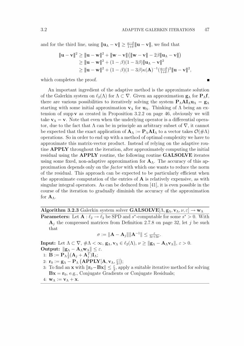
3.2 ADAPTIVE GALERKIN ITERATIONS 47
and for the third line, using |||uΛ − v||| ≥ α−δ1+δ
|||u− v|||, we find that
|||u− v|||2 ≥ |||u−w|||2 + |||w − v|||(|||w − v||| − 2β|||uΛ − v|||
)≥ |||u−w|||2 + (1− β)(1− 3β)|||uΛ − v|||2
≥ |||u−w|||2 + (1− β)(1− 3β)κ(A)−1(α−δ1+δ
)2|||u− v|||2,
which completes the proof.
An important ingredient of the adaptive method is the approximate solutionof the Galerkin system on `2(Λ) for Λ ⊂ ∇. Given an approximation gΛ for PΛf ,there are various possibilities to iteratively solving the system PΛAIΛuΛ = gΛ
starting with some initial approximation vΛ for uΛ. Thinking of Λ being an ex-tension of suppv as created in Proposition 3.2.2 on page 46, obviously we willtake vΛ = v. Note that even when the underlying operator is a differential opera-tor, due to the fact that Λ can be in principle an arbitrary subset of ∇, it cannotbe expected that the exact application of AΛ := PΛAIΛ to a vector takes O(#Λ)operations. So in order to end up with a method of optimal complexity we have toapproximate this matrix-vector product. Instead of relying on the adaptive rou-tine APPLY throughout the iteration, after approximately computing the initialresidual using the APPLY routine, the following routine GALSOLVE iteratesusing some fixed, non-adaptive approximation for AΛ. The accuracy of this ap-proximation depends only on the factor with which one wants to reduce the normof the residual. This approach can be expected to be particularly efficient whenthe approximate computation of the entries of A is relatively expensive, as withsingular integral operators. As can be deduced from [41], it is even possible in thecourse of the iteration to gradually diminish the accuracy of the approximationfor AΛ.
Algorithm 3.2.3 Galerkin system solver GALSOLVE[Λ,gΛ,vΛ, ν, ε] → wΛ
Parameters: Let A : `2 → `2 be SPD and s∗-computable for some s∗ > 0. WithAj the compressed matrices from Definition 2.7.8 on page 32, let j be suchthat
σ := ‖A−Aj‖‖A−1‖ ≤ ε3ε+3ν
.
Input: Let Λ ⊂ ∇, #Λ <∞, gΛ,vΛ ∈ `2(Λ), ν ≥ ‖gΛ −AΛvΛ‖, ε > 0.Output: ‖gΛ −AΛwΛ‖ ≤ ε.1: B := PΛ
12(Aj + AT
j )IΛ;
2: r0 := gΛ −PΛ
(APPLY[A,vΛ,
ε3]);
3: To find an x with ‖r0−Bx‖ ≤ ε3, apply a suitable iterative method for solving
Bx = r0, e.g., Conjugate Gradients or Conjugate Residuals;4: wΛ := vΛ + x.

48 ADAPTIVE GALERKIN METHODS 3.2
Proposition 3.2.4. Let A be s∗-computable for some s∗ > 0. Then wΛ :=GALSOLVE[Λ,gΛ,vΛ, ν, ε] terminates with ‖gΛ − AΛvΛ‖ ≤ ε, and for anys < s∗, the number of arithmetic operations and storage locations required by thecall is bounded by some absolute multiple of ε−1/s|vΛ|1/sAs + c(ν/ε)#Λ + 1, wherec : R>0 → R>0 is some non-decreasing function.
Proof. Using that 〈AΛzΛ, zΛ〉 ≥ ‖A−1‖−1‖vΛ‖2 for z ∈ `2(Λ), and ‖AΛ −B‖ ≤‖A − Aj‖ = σ‖A−1‖−1 < 1
3‖A−1‖−1, we infer that B is SPD with respect to
the canonical scalar product on `2(Λ), and that κ(B) . 1 uniformly in ε and ν.
Writing B−1 = (I −A−1Λ (AΛ −B))−1A−1
Λ , we find that ‖B−1‖ ≤ ‖A−1Λ ‖
1−‖A−1Λ ‖‖AΛ−B‖
and so ‖AΛ −B‖‖B−1‖ ≤ σ1−σ .
We have ‖r0‖ ≤ ν + ε3. Writing
gΛ −AΛwΛ = (gΛ −AΛvΛ − r0) + (r0 −Bx) + (B−AΛ)B−1(r0 + Bx− r0),
we find‖AΛwΛ − gΛ‖ ≤ ε
3+ ε
3+ σ
1−σ (ν + ε3
+ ε3) ≤ ε.
The s∗-computability of A show that the cost of the computation of r0 is boundedby some multiple of ε−1/s|vΛ|1/sAs +#Λ. Since B is sparse and can be constructed inO(#Λ) operations, and the required number of iterations of the iterative methodis bounded, everything only dependent on an upper bound for ν/ε, the proof iscomplete.
As announced in the introduction of this chapter, before introducing our adap-tive algorithm without coarsening of the iterands, we present an adaptive Galerkinalgorithm which, combined with coarsening of the iterands as in Algorithm 2.6.7on page 28, provides an optimal adaptive algorithm. We use the subroutine RESgiven in Algorithm 2.8.2 on page 37 for the computation of the approximateresiduals with sufficiently small relative errors.

3.2 ADAPTIVE GALERKIN ITERATIONS 49
Algorithm 3.2.5 Adaptive Galerkin method GALERKIN[v, ν0, ε] → vi
Parameters: Let 0 < δ < 1 and 0 < γ < 16κ(A)−
12 (1− δ). Let θ > 0 be a fixed
constant.Input: Let v ∈ P , ν0 ≥ ‖f −Av‖, and ε > 0.Output: vi ∈ P with ‖f −Avi‖ ≤ ε.1: i := 0, v1 := v;2: loop3: i := i+ 1;4: [ri, νi] := RES[vi, θνi−1, δ, ε], with L := A inside RES;5: if νi ≤ ε then6: Terminate the subroutine.7: end if8: Λi+1 := suppvi ∪ supp ri;9: gi+1 := PΛi+1
(RHS[f , γ‖ri‖]);10: vi+1 := GALSOLVE[Λi+1,gi+1,vi, γ‖ri‖+ νi, γ‖ri‖];11: end loop
Remark 3.2.6. Given vi, the index set Λi+1 is the same as the support of thenext iterand in an approximate steepest descent iteration. Although one couldapply Proposition 2.8.1 on page 37 to analyze its convergence, we use Proposition3.2.2 on page 46 to get a sharper result. It is clear that the above algorithmcorresponds to the case α = 1 in Proposition 3.2.2. In the next section, we willexplore the possibility α < 1.
Theorem 3.2.7. Let A be s∗-computable, and let f be s∗-admissible for somes∗ > 0. Then w := GALERKIN[v, ν0, ε] terminates with ‖f − Aw‖ ≤ ε.Moreover, the procedure ITERATE := GALERKIN with ‖ · ‖? := ‖A · ‖satisfies the conditions of Theorem 2.6.8 on page 28 for any s ∈ (0, s∗), meaningthat SOLVE presented in Algorithm 2.6.7 on page 28 using this ITERATEdefines an optimal adaptive algorithm for s ∈ (0, s∗).
Proof. From the properties of RES, for any vi determined inside the loop, withri := f −Avi, we have νi ≥ ‖ri‖, and either νi ≤ ε or ‖ri− ri‖ ≤ δ‖ri‖. We have‖PΛi+1
ri‖ ≥ α‖ri‖ with α = 1, Λi+1 ⊇ suppvi, and
‖gi+1 −PΛi+1Avi‖ ≤ ‖PΛi+1
(gi+1 − f)‖+ ‖PΛi+1(f −Avi)‖ ≤ γ‖ri‖+ νi.
As long as νi > ε, from (1− δ)‖ri‖ ≤ ‖ri‖ ≤ (1 + δ)‖ri‖ and νi ≤ (1 + δ)‖ri‖, wehave νi h ‖ri‖ h ‖ri‖, and Proposition 3.2.2 shows that |||u− vi+1||| ≤ ρ|||u− vi|||with some ρ ∈ [0, 1), or νi+1 . ρi−kνk for 0 ≤ k ≤ i+ 1. This proves that the

50 ADAPTIVE GALERKIN METHODS 3.2
loop terminates after a finite number of iterations, say directly after the K-thcall of RES.
As for the conditions of Theorem 2.6.8, recall that we need to prove that forany s ∈ (0, s∗) and for ε & ν0 ≥ ‖f −Av‖,
# suppw . # suppv + ε−1/s|u|1/sAs , |w|As . (# suppv)sε+ |u|As ,
and that the number of arithmetic operations and storage locations required bythis call of GALERKIN can be bounded by an absolute multiple of
ε−1/s|u|1/sAs + # suppv + 1.
These conditions are trivially true for K = 1, and from now on we will assumethat K > 1. For 1 ≤ i < K, from Proposition 2.3.6 on page 18 we have, withΛ1 := suppv1,
|vi|As . |u|As + (#Λi)sνi, (3.2.2)
and since #Λi+1−#Λi ≤ # supp ri for 1 ≤ i < K, by applying Proposition 2.8.4on page 38 we have, for 1 ≤ k < K,
#Λk+1 ≤ #Λ1 +∑k
i=1(#Λi+1 −#Λi)
. #Λ1 +∑k
i=1 ν−1/si
(|vi|1/sAs + |u|1/sAs
). #Λ1 + ν
−1/sk |u|1/sAs +
∑ki=1 #Λi,
(3.2.3)
where in the last line we have used (3.2.2) and the fact that νi is geometricallydecreasing.
We have νi & minθνi−1, ε & ε for 1 < i ≤ K. We claim that #Λk+1 . #Λ1+
ν−1/sk |u|1/sAs for 1 ≤ k < K, and prove it by induction. Since νi is geometrically
decreasing, using (3.2.3) we infer
#Λk+1 . #Λ1 + ν−1/sk |u|1/sAs +
∑ki=1
(#Λ1 + ν
−1/si−1 |u|
1/sAs
). k#Λ1 + ν
−1/sk |u|1/sAs ,
(3.2.4)
which proves the claim since we have K . 1 by the condition ε & ν0. This claim,together with (3.2.2) and νi h ε, proves the bounds on # suppw and |w|As .
Now it remains to bound the cost of the algorithm. For 1 ≤ i ≤ K, we have
|vi|1/sAs . |u|1/sAs + (#Λ1)ν1/si , (3.2.5)

3.2 ADAPTIVE GALERKIN ITERATIONS 51
from (3.2.2) with the help of (3.2.4) when K > 1. By Proposition 2.8.4 onpage 38, the cost of the i-th call of RES for 1 ≤ i ≤ K is bounded by
ν−1/si
(|vi|1/sAs + |u|1/sAs + ν
1/si−1(# suppvi + 1)
). ν
−1/si
(|u|1/sAs + (#Λi)ν
1/si + ν
1/si−1(#Λ1 + 1)
). ν
−1/si |u|1/sAs + (νi−1
νi)1/s(#Λ1 + 1),
where we used (3.2.2), # suppvi ≤ #Λi . #Λ1 +ν−1/si−1 |u|
1/sAs , and νi . νi−1. Now
taking into account that νi & ε & ν0 & νi−1, and summing over 1 ≤ i ≤ K, weconclude that the total cost of the K . 1 calls of RES is bounded by an absolute
multiple of ε−1/s|u|1/sAs + #Λ1 + 1.
By Proposition 2.8.4 and (3.2.5), we have supp ri . ν1/si |u|1/sAs +#Λ1. The cost
of the i-th iteration with the cost of RES removed, for 1 ≤ i < K, is boundedby an absolute multiple of
1 + #Λ1 + ν−1/si |u|1/sAs + ν
−1/si |vi|1/sAs + #Λi+1c(1 + 2νi
γ‖ri‖)
. 1 + #Λ1 + ν−1/si |u|1/sAs ,
where we have used νi h ‖ri‖, (3.2.5), (3.2.4), and c : R>0 → R>0 is the non-decreasing function from Proposition 3.2.4 on page 48. The proof is completedby summing the above cost over 1 ≤ i < K and using that K . 1.
Remark 3.2.8. Inside the call of [ri, νi] := RES[vi, θνi−1, δ, ε] that is made inGALERKIN, we search an approximation
ri,ζ := RHS[f , ζ/2]−APPLY[A,vi, ζ/2]
for ri := f − Avi with a ζ ≤ δ‖ri,ζ‖ that is as large as possible in order tominimize the support of ri,ζ outside suppvi. When i > 0, because of the precedingcalls of RHS and GALSOLVE, we have a set Λi ⊃ suppvi and a ri−1 with‖PΛi
ri‖ ≤ εi := γ‖ri−1‖. In this remark, we investigate whether it is possible tobenefit from this information to obtain an approximation for the residual withrelative error not exceeding δ whose support extends less outside suppvi.
Let rIi,ζ := PΛiri,ζ and rEi,ζ := P∇\Λi
ri,ζ , and similarly rIi and rEi . From
ζ2 ≥ ‖ri − ri,ζ‖2 = ‖rIi − rIi,ζ‖2 + ‖rEi − rEi,ζ‖2
≥ (‖rIi,ζ‖ − εi)2 + ‖rEi − rEi,ζ‖2,
we have
‖ri − rEi,ζ‖ = (‖rEi − rEi,ζ‖2 + ‖rIi ‖2)12 ≤ (ζ2 − (‖rIi,ζ‖ − εi)
2 + ε2i )12 =: ζ .

52 ADAPTIVE GALERKIN METHODS 3.3
So, alternatively, instead of ri,ζ , we may use rEi,ζ as an approximation for ri, and
thus stop the routine RES as soon as νi := ‖rEi,ζ‖+ ζ ≤ ε or ζ ≤ δ‖rEi,ζ‖, and userEi,ζ also for the determination of Λi+1. Since for any ζ and ri,ζ with rIi,ζ 6= 0 and
ζ < ‖ri,ζ‖ it holds that ζ‖ri,ζ‖ < ζ‖rEi,ζ‖ if εi is small enough, under this conditionthe alternative test is passed more easily. This may even be a reason to decreasethe parameter γ.
The approach discussed in this remark has been applied in the experimentsreported in [30].
3.3 Optimal complexity without coarsening of the iterands
Now we come to the main part of this chapter. So far we relied on coarsening ofthe iterands to control their support sizes. Below we will show that, after a smallchange, GALERKIN produces approximate solutions with optimal convergencerate without such coarsening.
In the following key lemma, it is shown that for sufficiently small µ andu ∈ As, for a set Λ as in Lemma 3.2.1 on page 45 that has minimal cardi-nality, #(Λ\ suppv) can be bounded in terms of ‖f −Av‖ and |u|As only, i.e.,independently of |v|As and the value of s∗ (cf. (3.2.3) on page 50 and [17, §4.2-4.3]).
Lemma 3.3.1. Let µ ∈ (0, κ(A)−12 ) be a constant, v ∈ P , and for some s > 0,
u ∈ As. Then the smallest set Λ ⊃ suppv with
‖PΛ(f −Av)‖ ≥ µ‖f −Av‖
satisfies
#(Λ\ suppv) . ‖f −Av‖−1/s|u|1/sAs . (3.3.1)
Proof. Let λ > 0 be a constant with µ ≤ κ(A)−12 (1 − ‖A‖λ2)
12 . Let N be
the smallest integer such that a best N -term approximation uN for u satisfies‖u− uN‖ ≤ λ|||u− v|||. Since |||u− v||| ≥ ‖A‖− 1
2‖f −Av‖, we have
N . ‖f −Av‖−1/s|u|1/sAs .
With Λ := suppv ∪ suppuN , the solution of PΛAuΛ = PΛf satisfies
|||u− uΛ||| ≤ |||u− uN ||| ≤ ‖A‖12‖u− uN‖ ≤ ‖A‖
12λ|||u− v|||,

3.3 OPTIMAL COMPLEXITY WITHOUT COARSENING 53
and so by Galerkin orthogonality, |||uΛ − v||| ≥ (1− ‖A‖λ2)12 |||u− v|||, giving
‖PΛ(f −Av)‖ = ‖PΛ(AuΛ −Av)‖ ≥ ‖A−1‖−12 |||uΛ − v|||
≥ ‖A−1‖−12 (1− ‖A‖λ2)
12 |||u− v|||
≥ κ(A)−12 (1− ‖A‖λ2)
12‖f −Av‖
≥ µ‖f −Av‖.
Since Λ ⊃ suppv, by definition of Λ we conclude that
#(Λ\ suppv) ≤ #(Λ\ suppv) ≤ N . ‖f −Av‖−1/s|u|1/sAs .
Before proceeding further, let us briefly describe how the above lemma can beused to prove the optimal convergence rate of the adaptive algorithm in an idealsetting. For some constant µ ∈ (0, κ(A)−
12 ) and i ∈ N0, we define Λi+1 to be the
smallest set with ‖PΛ(f −AuΛi)‖ ≥ µ‖f −AuΛi
‖, where Λ0 := ∅ and uΛiis the
Galerkin solution in the subspace `2(Λi). By Lemma 3.2.1 on page 45, we havea fixed error reduction: |||u − uΛi+1
||| ≤ ρ|||u − uΛi||| for i ∈ N0, with a constant
ρ < 1. Now assuming that u ∈ As with some s > 0, by the preceding lemma andthe geometric decrease of ‖f −AuΛi
‖ h |||u− uΛi|||, for i ∈ N0 we have
#Λk =∑k−1
i=0 #(Λi+1 \ Λi) .∑k−1
i=0 ‖f −AuΛi‖−1/s|u|1/sAs
. ‖f −AuΛk−1‖−1/s|u|1/sAs ,
or, ‖u − uΛk‖ . (#Λk)
−s|u|As , which, in view of the assumption u ∈ As, ismodulo some constant factor the best possible bound on the error.
In view of realizing the above discussed idea for an algorithm with an inexactevaluation of the residuals and an inexact solution of the Galerkin systems, wewill modify Algorithm 3.2.5 on page 49 so that in Line 8, the set Λi+1 ⊃ suppvi ischosen to be such that ‖PΛi+1
ri‖ ≥ α‖ri‖ with #(Λi+1 \suppvi) minimal modulosome constant factor. We define the following routine to perform the latter task.
Algorithm 3.3.2 Index set expansion RESTRICT[Λ, r, α] → Λ
Input: Λ ⊂ ∇, #Λ <∞, r ∈ P , α ∈ (0, 1).Output: Λ ⊇ Λ and ‖PΛr‖ ≥ α‖r‖.1: r := COARSE[r|∇\Λ,
√1− α2‖r‖];
2: Λ := Λ ∪ supp r.
Lemma 3.3.3. The output of Λ := RESTRICT[Λ, r, α] satisfies Λ ⊇ Λ and‖PΛr‖ ≥ α‖r‖. Moreover, the output satisfies
#Λ−#Λ . min#Λ−#Λ : ‖PΛr‖ ≥ α‖r‖ and ∇ ⊃ Λ ⊇ Λ, (3.3.2)

54 ADAPTIVE GALERKIN METHODS 3.3
and the number of arithmetic operations and storage locations needed for thisroutine can be bounded by an absolute multiple of #Λ + # supp r + 1.
Proof. We have ‖r − PΛr‖ = ‖r|∇\Λ − r‖ ≤√
1− α2‖r‖, which is equivalentto ‖PΛr‖ ≥ α‖r‖. The work bound immediately follows from Lemma 2.6.4 onpage 26. Since Λ ∩ supp r = ∅, by applying Lemma 2.6.4 we have
#Λ−#Λ = # supp r . min#Λ : ‖r|∇\Λ −PΛr|∇\Λ‖ ≤√
1− α2‖r‖= min#Λ : ‖r−PΛ∪Λr‖ ≤
√1− α2‖r‖,
and observing that the minimum is obtained when Λ ∩ Λ = ∅, the proof iscompleted.
Now we present our modification of Algorithm 3.2.5. Recall that Algorithm3.2.5 was intended for a reduction of the error with a fixed factor, to be used insidethe algorithm SOLVE from Chapter 2, i.e., Algorithm 2.6.7 on page 28. Themodification given below will be an optimal solver in its own as the forthcomingTheorem 3.3.5 shows.
Algorithm 3.3.4 Method SOLVE[ε] → vi without coarsening of the iterands
Parameters: Let 0 < δ < α < 1 and 0 < γ < 16κ(A)−
12 (α − δ). Let θ > 0 be a
fixed constant, and let ν0 > 0 and v = 0.Input: ε > 0.Output: vi ∈ P with ‖f −Avi‖ ≤ ε.Description: The body of this algorithm is identical to Algorithm 3.2.5 on
page 49, except that we replace the statement in Line 8 byΛi+1 := RESTRICT[Λi, ri, α];
Using perturbation arguments, we will prove that SOLVE has optimal com-putational complexity.
Theorem 3.3.5. Let A be s∗-computable, and let f be s∗-admissible for somes∗ > 0. Then uε := SOLVE[ε] terminates with ‖f −Auε‖ ≤ ε. In addition, let
the parameters inside SOLVE satisfy α+δ1−δ < κ(A)−
12 . If ν0 h ‖f‖ & ε, and for
some s < s∗, u ∈ As, then suppuε . ε−1/s|u|1/sAs and the number of arithmeticoperations and storage locations required by the call is bounded by some absolutemultiple of the same expression.
Proof. By the same reasoning in the proof of Theorem 3.2.7 on page 49, SOLVE[ε]terminates say, after K iterations, and with some ρ ∈ (0, 1), we have
νi . ρi−kνk for 0 ≤ k ≤ i ≤ K. (3.3.3)

3.4 NUMERICAL EXPERIMENT 55
Here we will use the notations from the proof of Theorem 3.2.7. With µ = α+δ1−δ ,
for 1 ≤ i < K let Λi+1 ⊃ suppvi be the smallest set with ‖PΛi+1ri‖ ≥ µ‖ri‖.
Then
µ‖ri‖ ≤ µ‖ri‖+ µδ‖ri‖ ≤ ‖PΛi+1ri‖+ µδ‖ri‖ ≤ ‖PΛi+1
ri‖+ (1 + µ)δ‖ri‖
or ‖PΛi+1ri‖ ≥ α‖ri‖. By the property (3.3.2) of RESTRICT we have #(Λi+1 \
suppvi) . #(Λi+1 \ suppvi). Since µ < κ(A)−12 by the condition on α and
δ, and ‖f − Avi‖ h νi, an application of Lemma 3.3.1 on page 52 shows that
#(Λi+1 \ suppvi) . ν−1/si |u|1/sAs .
Since with Λ1 := ∅, suppvi ⊆ Λi and Λi ⊂ Λi+1, for 1 ≤ k ≤ K by (3.3.1) wehave
# suppvk ≤ #Λk =k−1∑i=1
#(Λi+1\Λi) . (k−1∑i=1
ν−1/si )|u|1/sAs . ν
−1/sk−1 |u|
1/sAs . (3.3.4)
From |vk|As . |u|As + (# suppvk)s‖vk − u‖ (Proposition 2.3.6 on page 18), we
infer that |vk|As . |u|As .By Proposition 2.8.4 on page 38, the cost of the i-th call of RES for 1 ≤ i ≤ K
is bounded by an absolute multiple of
ν−1/si
(|vi|1/sAs + |u|1/sAs + ν
1/si−1(# suppvi + 1)
). ν
−1/si |u|1/sAs ,
where we used (3.3.4), and 1 . ν−1/sk−1 |u|
1/sAs by νk−1 . ν0 . ‖f‖ . |u|As .
The cost of the k-th call for k < K of the subroutines RESTRICT, RHSor GALSOLVE is bounded by an absolute multiple of #Λk+1 + # supp ri .ν−1/sk |u|1/sAs , ν
−1/sk |u|1/sAs , or ν
−1/sk (|vk|1/sAs + |u|1/sAs ) + #Λk+1 . ν
−1/sk |u|1/sAs , respec-
tively. From (3.3.3) and νK & minνK−1, ε & ε by Proposition 2.8.4, where thesecond inequality follows from νK−1 > ε when K > 0, and by assumption whenK = 0, the proof is completed.
3.4 Numerical experimentWe consider the variational formulation of the following problem of order 2t = 2on the interval [0, 1], i.e., n = 1, with periodic boundary conditions
−∆u+ u = f on R/Z. (3.4.1)
We define the right-hand side f by f(v) = 4v(12) +
∫ 1
0g(x)v(x)dx, with
g(x) = (16π2 + 1) cos(4πx)− 4 +
2x2, if x ∈ [0, 1/2),2(1− x)2, if x ∈ [1/2, 1],
(3.4.2)

56 ADAPTIVE GALERKIN METHODS 3.4
so that the solution u is given by
u(x) = cos(4πx) +
2x2, if x ∈ [0, 1/2),2(1− x)2, if x ∈ [1/2, 1],
(3.4.3)
see Figure 3.1.
0 0.1 0.2 0.3 0.4 0.5 0.6 0.7 0.8 0.9 1!1
!0.8
!0.6
!0.4
!0.2
0
0.2
0.4
0.6
0.8
1
x
Figure 3.1: The solution u is the sum of both functions illustrated.
We use the periodized B-spline wavelets of order d = 3 with d = 3 vanish-ing moments from [21] normalized in the H1(0, 1)-norm. The solution u is inHs+1(R/Z) only for s < 1
2. On the other hand, since u can be shown to be in
Bs+1p (Lp(R/Z)) for any s > 0 with 1
p= 1
2+ s, we deduce that the corresponding
discrete solution u is in As for any s < d−tn
= 2.Each entry of the infinite stiffness matrix A can be computed in O(1) opera-
tions. By applying the compression rules from [86], which are quoted in Theorem7.3.3 on page 127, we see that A is s∗-compressible with s∗ = t+ d = 4.
For developing a routine RHS, we split f = 〈f1, ·〉L2 + f2, where f1(x) =(16π2 + 1) cos(4πx) − 4. Correspondingly, we split f = f1 + f2, and given atolerance ε, we approximate both infinite vectors within tolerance ε/2 by, forsuitable `1(ε), `2(ε), dropping all coefficients with indices λ with |λ| > `1(ε) or|λ| > `2(ε), respectively.
From
|〈ψλ, f1〉L2| ≤ ‖ψλ‖L1(0,1) infp∈P2
‖f1 − p‖L∞(suppψλ),
‖ψλ‖L1(0,1) ≤ diam(suppψλ))12‖ψλ‖L2(0,1),
diam(suppψλ) = 5 · 2−|λ|,‖ψλ‖L2(0,1) = [4|λ|‖ψ′‖2
L2(R)/‖ψ‖2L2(R) + 1]−1,

3.4 NUMERICAL EXPERIMENT 57
where ψ is the “mother wavelet”, #λ : |λ| = k = 2k, and infp∈P2 ‖f1 −p‖L∞(suppψλ) ≤ (π
4diam(suppψλ))
3‖f ′′′1 ‖L∞(0,1)/3! (Jackson estimate), we find an
upper bound for the error√∑
|λ|>`1(ε) |〈ψλ, f1〉L2|2 which is h 2−4`1(ε). Setting
this upper bound equal to ε/2, and solving for `1(ε) gives an approximation forf1 of length h 2`1(ε) h ε−1/4. Note that in view of the admissibility assumptionwe made on f , a vector length h ε−1/2 would have been sufficient. Such a lengthwould have been found with wavelets that have 1 vanishing moment.
From
|〈ψλ, f2〉| ≤ (4 + ‖g − f1‖L1(suppψλ))‖ψλ‖L∞(0,1),
‖g − f1‖L1(suppψλ) ≤ 5 · 2−|λ|,‖ψλ‖L∞(0,1) = [2|λ|/2‖ψ‖L∞(R)/‖ψ‖L2(R)]‖ψλ‖L2(0,1),
#|λ| = k :12
is an interior point of suppψλ = 9,
and the fact that 〈ψλ, f2〉 vanishes when λ is not in any of these sets, we find
an upper bound for the error√∑
|λ|>`2(ε) |〈ψλ, f2〉|2 which is h 2−`2(ε)/2. Setting
this upper bound equal to ε/2 and solving for `2(ε) gives an approximation forf2 of length ≤ 9(`2(ε) + 1) = O(| log(ε)|+ 1), which is asymptotically even muchsmaller than the bound we found in the f1 case. Since each entry of f can becomputed in O(1) operations, in view of Definition 2.7.4 on page 30, we concludethat f is s∗-admissible with s∗ = 4.
We will compare the results of Algorithm 3.3.4 with those of Algorithm 2.6.7on page 28 that uses the subroutine RICHARDSON from Algorithm 2.7.6 onpage 31 as ITERATE, which we refer to as being the CDD2 method.
We tested our Algorithm 3.3.4 or CDD2 with parameters α = 0.4, δ =0.012618, and γ = 0.009581, or K = 5 and θ = 2.5, respectively. Inside theranges where the methods are proven to be of optimal computational complexity,these parameters are close to the values that give the best quantitative results.Actually, since these ranges result from a succession of worst case analyses, wemay expect that outside them, i.e., concerning Algorithm 3.3.4 for larger α, δand γ, more efficient algorithms are obtained. The numerical results, given inFigure 3.2 on the next page, illustrate the optimal computational complexity ofboth Algorithm 3.3.4 and CDD2. Note that the time measurements do not startat zero, but after 100 = 1 second. The results show that in this example thenew method needs less than a factor 1
10in computing time to achieve the same
accuracy.

58 ADAPTIVE GALERKIN METHODS 3.4
100 101 102 103
10!3
10!2
10!1
100
101
1
2
wall clock time
norm
of r
esid
ual
CDD2New method
Figure 3.2: Convergence histories

Chapter 4Using polynomial preconditioners
4.1 IntroductionIn this chapter, we carry on with considering the linear equation
Au = f , (4.1.1)
where A : `2 → `2 is an SPD matrix and f ∈ `2. As we saw in the foregoingchapters, the quantitative properties of the adaptive algorithms for solving thissystem depend on the condition number κ(A) := ‖A‖‖A−1‖, which in turndepends on the underlying wavelet basis. While constructing a wavelet basiswith favourable quantitative properties is a rather delicate task, preconditioningthe equation (4.1.1) without any reference to the original continuous problemseems an attractive possibility to improve the conditioning of the system. In thischapter, with a preconditioner S : `2 → `2 such that κ(SA) < κ(A), instead of(4.1.1) we will consider the following linear equation,
SAu = Sf . (4.1.2)
Apart from the diagonal one, perhaps the simplest preconditioner is the inverseof a finite section of the stiffness matrix A. One could use the LU -decompositionto preserve the symmetry. For instance, when the coarsest level functions ofthe wavelet basis adversely affect the condition of the system harmfully, one caninvert the stiffness matrix restricted to the coarsest level and use the inverse asa preconditioner. Since we can approximate the action of the stiffness matrix,the next idea would be to use polynomial preconditioners. In this chapter, weinvestigate the use of polynomial preconditioners.
This chapter is organized as follows. In the next section, we recall someresults on polynomial preconditioners and put forward ways to use them in our
59

60 USING POLYNOMIAL PRECONDITIONERS 4.2
setting. Then in Section 4.3, we show that the adaptive wavelet algorithms withpolynomial preconditioners are again of optimal computational complexity.
4.2 Polynomial preconditionersIn the context of linear algebraic equations, polynomial preconditioners have beenstudied extensively, see e.g. [1, 58, 70]. In this section, we recall some of theresults regarding common polynomial preconditioners and analyze them in oursetting.
Now the preconditioning matrix S is a polynomial in A, namely, we assumethat S = p(A) for some polynomial p of degree k ≥ 0. p(A) commutes A, thusp(A)A is symmetric. Moreover, if p is positive on the spectrum of A, p(A)A ispositive definite. To be more practical, if
‖I− p(A)A‖ ≤ ρ for some ρ < 1, (4.2.1)
then p(A)A is positive definite, and we have the bound
κ[p(A)A] ≤ 1 + ρ
1− ρ. (4.2.2)
Neumann series polynomials
A simple choice for p is a polynomial based on Neumann series. With someω ∈ (0, 2
‖A‖) and N := I− ωA, we have
(ωA)−1 = I + N + N2 + . . . ,
and truncating this series we define a polynomial preconditioner
pk(A) := ω(I + N + . . .+ Nk). (4.2.3)
One easily identifies the application of pk(A) with k iterations of a dampedRichardson method. As for (4.2.1), we have
‖I− pk(A)A‖ = ‖ω(Nk+1 + Nk+2 + . . .)A‖ = ‖Nk+1‖ ≤ ‖N‖k+1.
Min-max polynomials
If the coefficients of the preconditioning polynomial p are given, in general theaction of p(A) is computed using k applications of A. Therefore we shall try to

4.2 POLYNOMIAL PRECONDITIONERS 61
minimize the condition number (4.2.2) keeping k as small as possible. By firstcomplexifying `2 and then applying the spectral theorem, cf. [69], we have
‖p(A)Ax‖2 =
∫σ(A)
[p(λ)λ]2dEx,x(λ) ≤ ‖x‖2 · maxλ∈σ(A)
[p(λ)λ]2, (4.2.4)
where σ(A) is the spectrum and E is the spectral decomposition of A. Thisimmediately implies ‖p(A)A‖ ≤ max
λ∈σ(A)|p(λ)λ|. Similarly, we can estimate
‖[p(A)A]−1‖ ≤ maxλ∈σ(A)
∣∣[p(λ)λ]−1∣∣ =
(minλ∈σ(A)
|p(λ)λ|)−1
,
where we assumed that p is nonzero on the spectrum of A. Now let σ(A) ⊂ [c, d]with c, d > 0. Then we have
κ[p(A)A] ≤maxλ∈[c,d] |p(λ)λ|minλ∈[c,d] |p(λ)λ|
for p nonzero on [c, d]. (4.2.5)
We consider the problem of minimizing the above upper bound over the polyno-mials of degree k. Recall the following result from [1, 58].
Lemma 4.2.1. Let pk be the polynomial defined by
pk(λ)λ = 1−Ck(
d+c−2λd−c )
Ck(d+cd−c)
, (4.2.6)
where Ck is the k-th Chebyshev polynomial of the first kind. Then
maxλ∈[c,d] |pk(λ)λ|minλ∈[c,d] |pk(λ)λ|
=|Ck(d+cd−c)|+ 1
|Ck(d+cd−c)| − 1≤
maxλ∈[c,d] |q(λ)λ|minλ∈[c,d] |q(λ)λ|
for all q ∈ Pk[c, d], with equality if and only if q is a scalar multiple of pk.
With [c, d] as above, estimating the norm in (4.2.1) as in (4.2.4), we get
‖I− p(A)A‖ ≤ maxλ∈[c,d]
|1− p(λ)λ|. (4.2.7)
It turns out that the same polynomial pk from (4.2.6) minimizes the upper bound(4.2.7) over Pk[c, d], and these polynomials are called the min-max polynomi-als. Furthermore, with the min-max polynomial pk we have ‖I − pk(A)A‖ ≤|Ck(d+cd−c)|
−1 < 1 for k ≥ 0, ensuring the positive definiteness of pk(A)A.For min-max polynomials, the application of pk(A) is equivalent to k iterations
of the Chebyshev method. In light of this fact, the coefficients of the polynomialpk can be computed, e.g. using three term recurrences.

62 USING POLYNOMIAL PRECONDITIONERS 4.2
Least-squares polynomials
An alternative family of preconditioning polynomials can be obtained by mini-mizing some quadratic norm of 1−p(λ)λ instead of the uniform norm, cf. (4.2.7).With a positive weight function w : [c, d] → R>0, we consider the following mini-mization problem∫ d
c
|1− p(λ)λ|2w(λ)dλ→ min over p ∈ Pk[c, d]. (4.2.8)
We call the solution of this problem a least-squares polynomial. Unlike the min-max polynomial, the least-square polynomial is biased in its suppression of theeigenvalues of A. For example, when w ≡ 1, the larger eigenvalues are mappedcloser to 1 than the small ones. If the eigenvalue distribution of A were known,one could choose w to emphasize the dense parts of the spectrum.
We recall the following result from [58].
Lemma 4.2.2. Let si ∈ Pk+1[c, d], 0 ≤ i ≤ k+ 1, be orthonormal with respect tothe weight function w, normalized so that si(0) > 0 for 0 ≤ i ≤ k + 1. Assumethat each si, 0 ≤ i ≤ k + 1, obtains its maximum on [c, d] at c. Then withJk+1(µ, λ) :=
∑k+1j=0 sj(µ)sj(λ), the solution pk to the problem (4.2.8) is given by
pk(λ)λ = 1− Jk+1(0, λ)
Jk+1(0, 0), (4.2.9)
and pk(λ) > 0 for λ ∈ [c, d].
This lemma is applicable to a wide range of weights, including the Jacobiweights
wα,β(λ) = (d− λ)α(λ− c)β,
when α, β ≥ −12. In this case, the function Jk+1(0, ·) is a shifted and scaled Jacobi
polynomial, cf. [1]. Since the polynomial is known explicitly, the norm (4.2.1)can be estimated by using e.g. the estimate (4.2.7).
Approximate preconditioning
Since it is not possible to compute the application of A exactly, the action ofthe polynomial preconditioner p(A) must be approximated. For the approximateapplication of an s∗-computable matrix A with s∗ > 0, we distinguish betweentwo possibilities: (a) we can use the subroutine APPLY; or (b) we can applysome approximation Aj as in Definition 2.7.8. Let pk be the polynomial given

4.2 POLYNOMIAL PRECONDITIONERS 63
by pk(λ) = a0 + a1λ + . . . + akλk and let S = pk(A). We consider the following
algorithm which implements possibility (a).
Algorithm 4.2.3 Polynomial preconditioner PRECa[r, ξ] → d
Parameters: Let εi, i = 1, . . . , k, be such that∑k
i=1 εi‖A‖i−1 ≤ ξ‖r‖ and εi &ξ‖r‖.
Input: Let r ∈ P and ξ > 0.Output: d ∈ P and ‖Sr− d‖ ≤ ξ‖r‖.1: bk := akr;2: for i = k, . . . , 1 do3: bk−1 := ai−1r + APPLY[A, bi, εi];4: end for5: d := b0.
Correspondingly, possibility (b) suggests the following algorithm.
Algorithm 4.2.4 Polynomial preconditioner PRECb[r, ξ] → d
Parameters: Let J satisfy ‖A −AJ‖∑k
i=1 i|ai|‖A‖i−1 ≤ ξ and 2J . ξ−1/s, forsome s > 0, with AJ a compressed matrix as in Definition 2.7.8.
Input: Let r ∈ P and ξ > 0.Output: d ∈ P and ‖Sr− d‖ ≤ ξ‖r‖.1: bk := akr;2: for i = k, . . . , 1 do3: bk−1 := ai−1r + AJ bi;4: end for5: d := b0.
Definition 4.2.5. A subroutine PREC[r, ξ] → d is said to have linear complex-ity when for any ξ > 0 and a finite dimensional vector r ∈ `2, d := PREC[r, ξ]terminates with ‖Sr − d‖ ≤ ξ‖r‖, and for a non-increasing function c : R>0 →R>0, #suppd . c(ξ)#supp r and the number of arithmetic operations and stor-age locations required by the call being bounded by an absolute multiple ofc(ξ)#supp r + 1.
Proposition 4.2.6. Let A be s∗-computable with some s∗ > 0. Then the sub-routines PRECa[r, ξ] and PRECb[r, ξ] are both of linear complexity.
Proof. For the subroutine PRECa, the choice εi = ξ‖r‖k‖A‖i−1 , 1 ≤ i ≤ k, satisfies
the assumptions on the parameters εi. For the subroutine PRECb, we can chooseJ satisfying the first condition and ‖A−AJ‖ & ξ. Choosing s such that s < s∗,

64 USING POLYNOMIAL PRECONDITIONERS 4.2
we have 2−Js & ξ, thus J satisfies the second condition. With bk := akr, definebi−1 := ai−1r + Abi recursively for i = k, . . . , 1. Note that Sr = b0.
We consider PRECa first. From
bi−1 − bi−1 = APPLY[A, bi, εi]−Abi
= APPLY[A, bi, εi]−Abi + A(bi − bi),
we have‖bi−1 − bi−1‖ ≤ εi + ‖A‖‖bi − bi‖ for i = 1, . . . , k,
giving ‖d− Sr‖ = ‖b0 − b0‖ ≤∑k
i=1 εi‖A‖i−1 ≤ ξ‖r‖.Taking into account that ‖APPLY[A, ·, ε]‖ ≤ ‖A‖‖ · ‖+ ε for any ε > 0, and
εi . ξ‖r‖, we can derive that ‖bi‖ . ‖r‖ where the constant absorbed by ”.”possibly depends on ξ. For any x ∈ As, from (2.3.3) we have
|x|As = supNN s‖x− BN(x)‖ ≤ (# suppx)s‖x‖.
Accordingly, we infer
# supp bi−1 . # supp r + ε−1/si |bi|1/sAs . # supp r + ε
−1/si ‖bi‖1/s(# suppbi),
for i = 1, . . . , k. Employing this bound for i = k, . . . , 1, we obtain
# suppd = # supp b0
. # supp r(1 + ε
−1/s1 ‖r‖1/s + . . .+ ε
−1/s1 . . . ε
−1/sk ‖r‖k/s
).
We employ the assumption εi & ξ‖r‖ or ε−1i ‖r‖ . ξ−1 to conclude the first part
of the proof.Now we turn to the subroutine PRECb. We have for i = 0, . . . , k − 1
‖bi‖ ≤ |ai|‖r‖+ ‖AJ‖‖bi+1‖ ≤ |ai|‖r‖+ ‖A‖‖bi+1‖,
or ‖bi‖ ≤ ‖r‖∑k
j=i |aj|‖A‖j−i. On the other hand, we have for i = 1, . . . , k
‖bi−1 − bi−1‖ = ‖AJ bi −Abi‖ ≤ ‖AJ −A‖‖bi‖+ ‖A‖‖bi − bi‖≤ ‖AJ −A‖‖r‖
∑kj=i |aj|‖A‖j−i + ‖A‖‖bi − bi‖.
This yields
‖d− Sr‖ = ‖b0 − b0‖ ≤ ‖AJ −A‖‖r‖k∑i=1
‖A‖i−1
k∑j=i
|aj|‖A‖j−i
≤ ‖AJ −A‖‖r‖k∑j=1
j∑i=1
|aj|‖A‖j−1 ≤ ‖AJ −A‖‖r‖k∑j=1
j|aj|‖A‖j−1,

4.3 PRECONDITIONED ADAPTIVE ALGORITHM 65
where by assumption the last expression is bounded by ξ‖r‖.For the support size, we have # suppbi−1 . # supp r + 2J# suppbi, giving
that
# suppd = # suppb0 . (1 + 2J + . . .+ 2Jk)# supp r . 2Jk# supp r.
Finally, we use the assumption 2J . ξ−1/s to complete the proof.
4.3 Preconditioned adaptive algorithmThroughout this section, we assume that pk is a polynomial of degree k such thatS = pk(A) is positive definite and PREC[r, ξ] → d is an algorithm of linearcomplexity to approximate the action of S. We analyze here the preconditioningof the algorithm from the preceding chapter. First we define the routine forapproximately solving the preconditioned Galerkin system PΛSAuΛ = PΛSf ,with Λ ⊂ ∇.
Algorithm 4.3.1 Galerkin system solver GALSOLVE[Λ,vΛ, ν, η, ε] → wΛ
Parameters: Let A be s∗-computable for some s∗ > 0. With Aj the compressedmatrices from Definition 2.7.8, let J be such that
% := ‖SA− pk(AJ)AJ‖‖(SA)−1‖ ≤ α%ε
η+(1−α%)ε.
Let αd, αr, αg, α% > 0 be constants such that αd+αr+αg+α% = 1 and α% ≤ 12.
Input: Let Λ ⊂ ∇, #Λ < ∞, vΛ ∈ `2(Λ), ε > 0, ν ≥ ‖f − AvΛ‖ and η ≥‖PΛS(f −AvΛ)‖.
Output: wΛ ∈ `2(Λ) and ‖PΛS(f −AwΛ)‖ ≤ ε.1: B := PΛ
12[pk(AJ)AJ + pk(A
∗J)A
∗J ] IΛ;
2: r := RHS[f , εr
2]−APPLY[A,vΛ,
εr
2] with εr := αrνε
αdε+ν‖S‖;
3: d := PΛ
(PREC[r, αdε
ν]);
4: To find an x with ‖d − Bx‖ ≤ αgε, apply a suitable iterative method forsolving Bx = d, e.g., Conjugate Gradients or Conjugate Residuals;
5: wΛ := vΛ + x.
Proposition 4.3.2. Let A be s∗-computable, and let f be s∗-admissible for somes∗ > 0. Then wΛ := GALSOLVE[Λ,vΛ, ν, η, ε] terminates with ‖PΛS(f −AwΛ)‖ ≤ ε, and for any s < s∗, the number of arithmetic operations and storage
locations required by the call is bounded by an absolute multiple of ε−1/s(|vΛ|1/sAs +
|u|1/sAs ) + c(η/ε)#Λ, with c : R>0 → R>0 being some non-decreasing function.

66 USING POLYNOMIAL PRECONDITIONERS 4.3
Proof. Since the proof of Proposition 3.2.4 works for this proposition with slightadjustments, we comment here only on some points. From ‖SA− pk(AJ)AJ‖ ≤%‖(SA)−1‖−1, we imply that B is SPD, and that κ(B) . 1 uniformly in η and ε.To prove the first claim of the theorem, one can use
‖PΛS(f −Aw)− d‖ = ‖PΛS(f −Aw − r) + PΛSr− d‖ ≤ ‖S‖εr + ξ‖r‖,
and ‖r‖ ≤ ν + εr. B is sparse, and thus the work bound follows.
Algorithm 4.3.3 Preconditioned adaptive method SOLVE[ν0, ε] → vi
Parameters: Let α, δ, and ξ be some positive constants such that with δ :=δ‖S‖+ξ
‖S−1‖−1−ξ , 0 < δ < α < 1 and α+δ1−δ < κ(SA)−
12 . Let 0 < γ < 1
3κ(SA)−
12 (α− δ)
and θ > 0 be constants.Input: Let ν0 & ε > 0.Output: vi ∈ P and ‖f −Avi‖ ≤ νi ≤ ε.1: i := 0, v1 := 0;2: loop3: i := i+ 1;4: [ri, νi] := RES[vi, θνi−1, δ, ε];5: if νi ≤ ε then6: Terminate the subroutine.7: end if8: di := PREC[ri, ξ];9: Λi+1 := RESTRICT[suppvi, di, α];
10: ηi := ‖di‖+ (ξ + δ‖S‖)‖ri‖;11: vi+1 := GALSOLVE[Λi+1,vi, νi, ηi, γ‖di‖];12: end loop
We now define the preconditioned adaptive wavelet solver.
Theorem 4.3.4. Let A be s∗-computable, and let f be s∗-admissible for somes∗ > 0. Then uε := SOLVE[ν0, ε] terminates with ‖f −Auε‖ ≤ ε. Moreover, if
ν0 h ‖f‖ & ε, and for some s < s∗, u ∈ As, then # suppuε . ε−1/s|u|1/sAs andthe number of arithmetic operations and storage locations required by the call isbounded by some absolute multiple of the same expression.
Proof. From the properties of RES, for any vi determined inside the loop, withri := f − Avi, we have νi ≥ ‖ri‖, and either νi ≤ ε or ‖ri − ri‖ ≤ δ‖ri‖.Moreover, we have νi & minθνi−1, ε & ε for i ≥ 1. Now suppose that for ani > 0, RES terminates with νi > ε and thus with ‖ri − ri‖ ≤ δ‖ri‖. Then from

4.3 PRECONDITIONED ADAPTIVE ALGORITHM 67
(1− δ)‖ri‖ ≤ ‖ri‖ ≤ (1 + δ)‖ri‖ and νi ≤ (1 + δ)‖ri‖, we have νi h ‖ri‖ h ‖ri‖,and
‖Sri − di‖ = ‖S(ri − ri) + Sri − di‖ ≤ ‖S‖δ‖ri‖+ ξ‖ri‖,
so ηi is an upper bound on ‖Sri‖. Furthermore, we have
‖ri‖ ≤ ‖S−1‖‖Sri‖ ≤ ‖S−1‖(‖di‖+ ξ‖ri‖
),
implying that ‖Sri − di‖ ≤ δ‖di‖ and ηi ≤ (1 + δ)‖di‖. Similarly to the abovecase with νi, we now infer ηi h ‖di‖ h ‖Sri‖, and since ‖Sri‖ h ‖ri‖, we have
ηi h νi. With the norm |||·||| := 〈SA·, ·〉 12 which is equivalent to the standard norm
‖·‖ on `2, Proposition 3.2.2 shows that |||u−vi+1||| ≤ ρ|||u−vi||| for some ρ ∈ [0, 1),or νi+1 . ρi−kνk for 0 ≤ k ≤ i+ 1. This proves that the loop terminates after afinite number of iterations, say directly after the K-the call of RES.
Since PREC is of linear complexity we have # supp di . # supp ri, and thecost of the i-th call of PREC is of order # supp ri + 1. The rest of the proof iscompletely analogous to the analysis in the proof of Theorem 3.3.5.

68 USING POLYNOMIAL PRECONDITIONERS 4.3

Chapter 5Adaptive algorithm for nonsymmetric andindefinite elliptic problems
5.1 IntroductionLet H be a real Hilbert space and let H′ denote its dual. Given a boundedlyinvertible linear operator L : H → H′ and a linear functional f ∈ H′, we considerthe problem of finding u ∈ H such that
Lu = f.
As an example of H one can think of the Sobolev space H t on a domain ormanifold, possibly incorporating essential boundary conditions. Then the weakformulation of (scalar) linear differential or integral equations of order 2t leads tothe above type of equations.
Let Ψ = ψλ ∈ H : λ ∈ ∇ be a Riesz basis of wavelet type for H with acountable index set ∇. We consider Ψ formally as a column vector whose entriesare elements of H. Let u = uTΨ with u a column vector in `2 := `2(∇). Then, aswe already have seen, the above problem is equivalent to finding u ∈ `2 satisfyingthe infinite matrix-vector system
Lu = f , (5.1.1)
where L := 〈ψλ, Lψµ〉λ,µ∈∇ : `2 → `2 is boundedly invertible and f := 〈f, ψλ〉λ∈∇ ∈`2. Here 〈·, ·〉 denotes the duality product on H×H′.
In the foregoing chapters, we have encountered a number of adaptive methodsfor solving the above type of equations. The methods apply under the conditionthat L is symmetric, positive definite (SPD), which is equivalent to 〈Lv,w〉 =〈v, Lw〉, v, w ∈ H, and 〈Lv, v〉 & ‖v‖2
H, v ∈ H, i.e., that L is self-adjoint and
69

70 EXTENSION TO STRONGLY ELLIPTIC OPERATOR EQUATIONS 5.2
H-elliptic. For the case that L does not have both properties, as was suggestedin [18], one can reformulate Lu = f as an equivalent well-posed infinite matrix-vector problem with a symmetric, positive definite system matrix, as via thenormal equations, or, in case the equation represents a saddle point problem, byusing the reformulation as a positive definite system introduced in [10].
Throughout this chapter, we will consider the operators of type L = A + Bwhere A is self-adjoint and H-elliptic, and B is compact. Now in general L isno longer SPD, hence the above mentioned adaptive wavelet methods cannotbe applied directly. One can consider the normal equation LTLu = LT f ; how-ever, the main disadvantage of this approach is that the condition number ofthe system is squared, while the quantitative properties of the methods dependsensitively on the conditioning of the system. In this chapter, we will modifythe adaptive wavelet algorithm from Chapter 3 so that it applies directly to thesystem Lu = f , avoiding the normal equations. The analysis in Chapter 3 ex-tensively uses the Galerkin orthogonality, which in the present case has to bereplaced by only a quasi-orthogonality property. It should be mentioned that thisquasi-orthogonality property has been used in [62] in a convergence proof of anadaptive finite element method. By proving the quasi-orthogonality property forthe present general setting and extending the complexity analysis in Chapter 3,we will show that our algorithm has optimal computational complexity.
This chapter is organized as follows. In the following section, we derive resultson Ritz-Galerkin approximations to the exact solution, and in the last section,the adaptive wavelet algorithm is constructed and analyzed.
5.2 Ritz-Galerkin approximationsLet H → Y be separable real Hilbert spaces with compact embedding, and leta : H×H → R and b : Y ×H → R be bounded bilinear forms. We assume thatthe bilinear form a is symmetric and elliptic, which implies that ||| · ||| := a(·, ·) 1
2
is an equivalent norm on H, i.e.,
|||v||| h ‖v‖H v ∈ H. (5.2.1)
In particular, the operator A : H → H′ defined by 〈Av,w〉 = a(v, w) for v, w ∈ H,is boundedly invertible. Moreover, since B : H → H′ defined by 〈Bv,w〉 = b(v, w)for v, w ∈ H, is compact, the linear operator L := A+B is a Fredholm operatorof index zero. Therefore, assuming that L is injective, L : H → H′ is boundedlyinvertible, in particular meaning that the linear operator equation
Lu = f, (5.2.2)
has a unique solution for f ∈ H′.

5.2 RITZ-GALERKIN APPROXIMATIONS 71
For our analysis we will need the following mild regularity assumption on theadjoint L′ of L: There is a Hilbert space X → H with compact embedding, suchthat (L′)−1 : Y ′ → X is bounded. The following lemma gives a means to checkthis assumption.
Lemma 5.2.1. Let either A−1 : Y ′ → X or L−1 : Y ′ → X be bounded. Then(L′)−1 : Y ′ → X is bounded.
Proof. We treat the first case only. The other case is analogous. The operatorB extends to a bounded mapping from Y to H′. So L′ = A + B′ : X → Y ′ isbounded. Now consider the equation L′u = f . We know that there exists a uniquesolution u ∈ H with ‖u‖H . ‖f‖H′ and thus ‖B′u‖Y ′ . ‖u‖H . ‖f‖H′ . ‖f‖Y ′ .From Au = f −B′u, we now infer that ‖u‖X . ‖f‖Y ′ .
Example 5.2.2. For some Lipschitz domain Ω ⊂ Rn, with H := H10 (Ω) let
L : H → H′ be defined by
〈Lv,w〉 = −n∑
j,k=1
〈ajk∂kv, ∂jw〉L2 +n∑k=1
〈bk∂kv, w〉L2 + 〈cv, w〉L2 v, w ∈ H.
If the coefficients satisfy ajk, bk, c ∈ L∞ then L : H → H′ is bounded. Moreover,if the matrix [ajk] is symmetric and uniformly positive definite a.e. in Ω, then thebilinear form a(·, ·) := −
∑nj,k=1〈ajk∂k·, ∂j·〉L2 is symmetric and satisfies (5.2.1).
If either bk = 0, 1 ≤ k ≤ n and c ≥ 0 a.e. or c ≥ β > 0 a.e., then the generalizedmaximum principle implies that L is injective, cf. [81]. Also if L = A − η2
for a constant η ∈ R, then the injectivity is guaranteed as long as η2 is notan eigenvalue of A. With Yσ := (L2(Ω), H1
0 (Ω))1−σ,2 for some σ ∈ (0, 1], where(X, Y )θ,p denotes the intermediate space between X and Y obtained by the realinterpolation method, the bilinear form b(·, ·) :=
∑nk=1〈bk∂k·, ·〉L2 + 〈c·, ·〉L2 :
Yσ ×H → R is bounded for any σ ∈ (0, 1]. If the coefficients ajk, 1 ≤ j, k ≤ n,are Lipschitz continuous, then with Xσ := (H1
0 (Ω), H2(Ω)∩H10 (Ω))σ,2 it is known
that A−1 : Y ′σ → Xσ is bounded for any σ ∈ (0, 1
2), cf. [75]. Furthermore, the
embeddings Xσ → H → Yσ are compact. From Lemma 5.2.1 we conclude thatall aforementioned conditions are satisfied.
Example 5.2.3. Let L be the operator considered in the above example. Weassume that the domain Ω is Lipschitz, the coefficients ajk, bk, c are constant andthat the matrix [ajk] is symmetric and positive definite. Then the single layerand hypersingular boundary integral operators corresponding to the differentialoperator L can be written as the sum of a boundedH-elliptic operatorA : H → H′
and a compact operator B : H → H′, see [23]. With Γ being the boundary of theunderlying domain Ω, here the energy space is H = H t(Γ) with t = −1
2for the

72 EXTENSION TO STRONGLY ELLIPTIC OPERATOR EQUATIONS 5.2
single layer operator and t = 12
for the hypersingular integral operator. A closeinspection of the proofs of [24, Theorem 3.9] and [23, Theorem 2] reveals that inboth cases, the operator A is self-adjoint and that with Yσ := H t−σ(Γ) where thas the appropriate value depending on the case, the operator B can be extendedto a bounded operator Yσ → H′ for any σ ∈ (0, 1
2]. Assuming the injectivity
of L : H → H′, in [23] it is shown that with Xσ := H t+σ(Γ), L−1 : Y ′σ → Xσ
is bounded for any σ ∈ [0, 12]. The injectivity depends on the particular case at
hand, see [61] for some important cases.
We consider a sequence of finite dimensional closed subspaces V0 ⊂ V1 ⊂ . . . ⊂H satisfying
infvj∈Vj
‖v − vj‖H ≤ αj‖v‖X v ∈ X , (5.2.3)
with limj→∞ αj = 0.
Remark 5.2.4. Such a sequence exists since the embedding X → H is compact,cf. [77].
Example 5.2.5. Let H = H t and X = H t+σ. Then for standard finite elementor spline spaces Vj subordinate to dyadic subdivisions of an initial mesh, theapproximation property (5.2.3) is satisfied with αj h 2−jσ, for any t < γ andσ ≤ d − t, where d is the polynomial order of the spaces Vj, and γ = supjs :Vj ⊂ Hs, see e.g. [64].
For a finite dimensional closed subspace S ⊂ H such that Vj ⊆ S for some j,we consider the Ritz-Galerkin problem
〈LuS, vS〉 = 〈f, vS〉 for all vS ∈ S. (5.2.4)
It is well known that for j being sufficiently large, a unique solution uS tothe above problem exists, and that uS is a near best approximation to u in theenergy norm ||| · |||. In the weaker norm ‖ · ‖Y , convergence of higher order than(5.2.3) can be obtained via an Aubin-Nitsche duality argument, cf. [76]. Theseresults are recalled in the following lemma, where for convenience we also includea proof.
Lemma 5.2.6. There is an absolute constant j0 ∈ N0 (not depending on S) suchthat for all j ≥ j0, (5.2.4) has a unique solution with
|||u− uS||| ≤ [1 +O(αj)] infv∈S
|||u− v|||. (5.2.5)
Moreover, for j ≥ j0 we have
‖u− uS‖Y ≤ O(αj)|||u− uS|||. (5.2.6)

5.2 RITZ-GALERKIN APPROXIMATIONS 73
Proof. Suppose that a solution uS to (5.2.4) exists. Then we trivially have
〈L(u− uS), vS〉 = 0 ∀vS ∈ S. (5.2.7)
Using this and the boundedness of b : Y ×H → R, for arbitrary vS ∈ S we get
|||u− uS|||2 = 〈L(u− uS), u− uS〉 − b(u− uS, u− uS)
= 〈L(u− uS), u− vS〉 − b(u− uS, u− uS)
= a(u− uS, u− vS) + b(u− uS, uS − vS)
≤ |||u− uS||||||u− vS|||+O(1)‖u− uS‖Y‖uS − vS‖H.
(5.2.8)
We estimate ‖u − uS‖Y by an Aubin-Nitsche duality argument. For w ∈ Y ′ weinfer that
〈u− uS, w〉 = 〈L(u− uS), (L′)−1w − wS〉
≤ ‖L‖H→H′‖u− uS‖H‖(L′)−1w − wS‖H≤ ‖L‖H→H′‖u− uS‖Hαj‖(L′)−1w‖X≤ ‖L‖H→H′‖u− uS‖Hαj‖(L′)−1‖Y ′→X‖w‖Y ′ ,
where we used (5.2.7), (5.2.3) and the boundedness of (L′)−1 : Y ′ → X . We have
‖u− uS‖Y = supw∈Y ′
〈u− uS, w〉‖w‖Y ′
,
and subsequently using (5.2.1) we arrive at (5.2.6). Substituting (5.2.6) into(5.2.8), we get
|||u− uS||| ≤ |||u− vS|||+O(αj)‖uS − vS‖H.
For the last term, from the triangle inequality and (5.2.1), we have
‖v − uS‖H . |||u− uS|||+ |||u− vS|||.
Now choosing j0 sufficiently large, we finally obtain (5.2.5).Since (5.2.4) is a finite dimensional system, existence and uniqueness are
equivalent. To see the uniqueness, it is sufficient to prove that f = 0 impliesuS = 0. By linearity and invertibility of L, we have u = 0 if f = 0, and so (5.2.5)implies that uS = 0. The proof is completed.
The following observation concerning quasi-orthogonality is an easy general-ization of [62, Lemma 2.1].

74 EXTENSION TO STRONGLY ELLIPTIC OPERATOR EQUATIONS 5.2
Lemma 5.2.7. For some j ≥ j0 with j0 being the absolute constant from Lemma5.2.6, let S0 ⊂ S1 ⊂ H be finite dimensional subspaces satisfying Vj ⊆ S0. Letu0 ∈ S0 and u1 ∈ S1 be the solutions to the Galerkin problems 〈Lu0, v〉 = 〈f, v〉∀v ∈ S0 and 〈Lu1, v〉 = 〈f, v〉 ∀v ∈ S1, respectively. Then we have∣∣|||u− u0|||2 − |||u− u1|||2 − |||u1 − u0|||2
∣∣ ≤ O(αj)(|||u− u0|||2 + |||u− u1|||2
).
(5.2.9)
Proof. We have |||u− u0|||2 = |||u− u1|||2 + |||u1 − u0|||2 + 2a(u− u1, u1 − u0). Using(5.2.7), boundedness of b : Y ×H → R, and the triangle inequality, we estimatethe absolute value of the last term as
|2a(u− u1, u1 − u0)| = |2b(u− u1, u1 − u0)|. ‖u− u1‖Y‖u1 − u0‖H≤ ‖u− u1‖Y (‖u− u1‖H + ‖u− u0‖H)
Now using (5.2.6), and applying the inequality 2ab ≤ a2+b2, a, b ∈ R, we concludethe proof by
|2a(u− u1, u1 − u0)| ≤ O(αj)(|||u− u1|||2 + |||u− u1||||||u− u0|||
)≤ O(αj)
(|||u− u1|||2 + |||u− u0|||2
).
Using a Riesz basis for H, we will now transform (5.2.2) into an equivalentinfinite matrix-vector system in `2. Let Ψ = ψλ : λ ∈ ∇ be a Riesz basis forH of wavelet type. We assume that for some ∇0 ⊂ ∇1 ⊂ . . . ⊂ ∇, the subspacesdefined by Vj = spanψλ : λ ∈ ∇j, j ∈ N0, satisfies (5.2.3) with limj→∞ αj = 0.
Example 5.2.8. With the spaces Vj described in Example 5.2.5, wavelet basessatisfying the above condition have been constructed e.g. in [14, 22, 33, 34, 56,85].
Writing u = uTΨ for some u ∈ `2, u satisfies
Lu = f , (5.2.10)
where L := 〈ψλ, Lψµ〉λ,µ∈∇ : `2 → `2 is boundedly invertible and f := 〈f, ψλ〉λ∈∇ ∈`2. Similarly to L, we define also the matrices
A := 〈ψλ, Aψµ〉λ,µ∈∇ = a(ψµ, ψλ)λ,µ∈∇ and
B := 〈ψλ, Bψµ〉λ,µ∈∇ = b(ψµ, ψλ)λ,µ∈∇,
so that L = A + B. The matrix A is symmetric positive definite, so 〈A·, ·〉 is aninner product on `2, and the induced norm ||| · ||| satisfies
|||v|||2 := 〈Av,v〉 = a(vTΨ,vTΨ) = |||vTΨ|||2 v ∈ `2.

5.2 RITZ-GALERKIN APPROXIMATIONS 75
Furthermore, one can verify that for any v ∈ `2, Λ ⊆ ∇, vΛ ∈ `2(Λ),
‖Av‖ ≤ ‖A‖12 |||v||| ≤ ‖A‖‖v‖, |||vΛ||| ≤ ‖A−1‖
12‖PΛAIΛvΛ‖, (5.2.11)
where PΛ : `2 → `2(Λ) is the orthogonal projector onto `2(Λ), and IΛ de-notes the trivial inclusion `2(Λ) → `2. For any v,w ∈ `2, we have 〈Bv,w〉 =b(vTΨ,wTΨ) . ‖vTΨ‖Y‖wTΨ‖H . ‖vTΨ‖Y‖w‖, implying the following esti-mate which will be used often in the rest of this section.
‖Bv‖ = sup0 6=w∈`2
〈Bv,w〉‖w‖
. ‖vTΨ‖Y v ∈ `2. (5.2.12)
For some Λ ⊂ ∇, let S = spanψλ : λ ∈ Λ ⊂ H. Then uS = (IΛuΛ)TΨ ∈ Sis the solution to the Galerkin problem (5.2.4) if and only if uΛ ∈ `2(Λ) satisfies
PΛLIΛuΛ = PΛf . (5.2.13)
In the following, we will refer to uΛ as the Galerkin solution with respect to theindex set Λ. From Lemma 5.2.6 we know that this solution exists and is uniquewhen ∇j ⊆ Λ for some j ≥ j0.
Lemma 5.2.9. Let PΛ and IΛ be as above. Then for any Λ ⊇ ∇j for somej ≥ j0 we have
‖(PΛLIΛ)−1‖ ≤ ‖A−1‖[1 + ‖BL−1‖+O(αj)
].
Proof. Recalling that L(u− uΛ) ⊥ `2(Λ) and that A = L−B, we have
‖uΛ‖2 ≤ ‖A−1‖|||uΛ|||2 = ‖A−1‖ [〈LuΛ,uΛ〉 − 〈BuΛ,uΛ〉]= ‖A−1‖ [〈Lu,uΛ〉 − 〈Bu,uΛ〉+ 〈B(u− uΛ),uΛ〉] .
Here and in the following, we write uΛ to mean IΛuΛ as well, i.e., uΛ is extended byzeros outside the index set Λ. Now applying the Cauchy-Bunyakowsky-Schwarzinequality gives
‖uΛ‖ ≤ ‖A−1‖ [‖Lu‖+ ‖Bu‖+ ‖B(u− uΛ)‖] . (5.2.14)
For the last term in the brackets, using the estimates (5.2.12), (5.2.6) and (5.2.5),we have
‖B(u− uΛ)‖ . ‖u− uTΛΨ‖Y ≤ O(αj)|||u− uTΛΨ|||≤ O(αj) inf
v∈`2(Λ)|||u− v||| ≤ O(αj)‖u‖.

76 EXTENSION TO STRONGLY ELLIPTIC OPERATOR EQUATIONS 5.2
We substitute it into (5.2.14) to get
‖uΛ‖ ≤ ‖A−1‖ [‖Lu‖+ ‖Bu‖+O(αj)‖u‖]≤ ‖A−1‖
[1 + ‖BL−1‖+O(αj)‖L−1‖
]‖f‖.
Since this estimate holds in particular for arbitrary f = PΛf , taking into accountthat uΛ = (PΛLIΛ)−1PΛf the proof is completed.
The following lemma generalizes Lemma 3.2.1 to the present case of nonsym-metric and indefinite operators, and provides a way to extend a given set Λ0 ⊂ ∇such that the error of the Galerkin solution with respect to the extended set isreduced by a constant factor.
Lemma 5.2.10. Suppose that u0 ∈ `2(Λ0) is the solution to PΛ0LIΛ0u0 = PΛ0fwith Λ0 ⊇ ∇j for j sufficiently large. For a constant µ ∈ (0, 1), let ∇ ⊃ Λ1 ⊃ Λ0
be such that‖PΛ1(f − Lu0)‖ ≥ µ‖f − Lu0‖. (5.2.15)
Then, for u1 ∈ `2(Λ1) being the solution to PΛ1LIΛ1u1 = PΛ1f , it holds that
|||u− u1||| ≤[1− κ(A)−1µ2 +O(αj)
] 12 |||u− u0|||.
Proof. In this proof, we use the notations u0 = uT0 Ψ and u1 = uT1 Ψ. We have
‖L(u1 − u0)‖2 = ‖A(u1 − u0)‖2 + 2〈A(u1 − u0),B(u1 − u0)〉+ ‖B(u1 − u0)‖2.
The first term on the right hand side is bounded from above by using the firstinequality from (5.2.11). We estimate the second term by using (5.2.12) as
|2〈A(u1 − u0),B(u1 − u0)〉| ≤ 2‖A(u1 − u0)‖‖B(u1 − u0)‖. |||u1 − u0|||‖u1 − u0‖Y .
For the third term we have ‖B(u1 − u0)‖2 . ‖u1 − u0‖2Y . Combining these
estimates, and taking into account (5.2.6), we conclude that
‖L(u1 − u0)‖2 ≤ ‖A‖|||u1 − u0|||2 +O(1)|||u1 − u0|||‖u1 − u0‖Y (5.2.16)
≤ ‖A‖|||u1 − u0|||2 +O(αj)(|||u− u0|||2 + |||u− u1|||2
).
On the other hand, we have
‖L(u− u0)‖2 = ‖A(u− u0)‖2 + 2〈A(u− u0),B(u− u0)〉+ ‖B(u− u0)‖2.
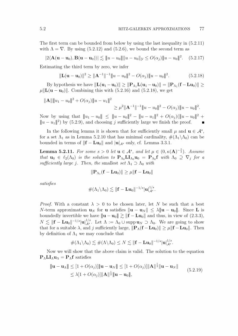
5.2 RITZ-GALERKIN APPROXIMATIONS 77
The first term can be bounded from below by using the last inequality in (5.2.11)with Λ = ∇. By using (5.2.12) and (5.2.6), we bound the second term as
|2〈A(u− u0),B(u− u0)〉| . |||u− u0|||‖u− u0‖Y ≤ O(αj)|||u− u0|||2. (5.2.17)
Estimating the third term by zero, we infer
‖L(u− u0)‖2 ≥ ‖A−1‖−1|||u− u0|||2 −O(αj)|||u− u0|||2. (5.2.18)
By hypothesis we have ‖L(u1−u0)‖ ≥ ‖PΛ1L(u1−u0)‖ = ‖PΛ1(f −Lu0)‖ ≥µ‖L(u− u0)‖. Combining this with (5.2.16) and (5.2.18), we get
‖A‖|||u1 − u0|||2 +O(αj)|||u− u1|||2
≥ µ2‖A−1‖−1|||u− u0|||2 −O(αj)|||u− u0|||2.
Now by using that |||u1 − u0||| ≤ |||u− u0|||2 − |||u− u1|||2 + O(αj)(|||u− u0|||2 +|||u− u1|||2) by (5.2.9), and choosing j sufficiently large we finish the proof.
In the following lemma it is shown that for sufficiently small µ and u ∈ As,for a set Λ1 as in Lemma 5.2.10 that has minimal cardinality, #(Λ1\Λ0) can bebounded in terms of ‖f − Lu0‖ and |u|As only, cf. Lemma 3.3.1.
Lemma 5.2.11. For some s > 0 let u ∈ As, and let µ ∈ (0, κ(A)−12 ). Assume
that u0 ∈ `2(Λ0) is the solution to PΛ0LIΛ0u0 = PΛ0f with Λ0 ⊇ ∇j for asufficiently large j. Then, the smallest set Λ1 ⊃ Λ0 with
‖PΛ1(f − Lu0)‖ ≥ µ‖f − Lu0‖
satisfies#(Λ1\Λ0) . ‖f − Lu0‖−1/s|u|1/sAs .
Proof. With a constant λ > 0 to be chosen later, let N be such that a bestN -term approximation uN for u satisfies ‖u − uN‖ ≤ λ|||u − u0|||. Since L isboundedly invertible we have |||u− u0||| & ‖f −Lu0‖ and thus, in view of (2.3.3),
N . ‖f − Lu0‖−1/s|u|1/sAs . Let Λ := Λ0 ∪ suppuN ⊃ Λ0. We are going to showthat for a suitable λ, and j sufficiently large, ‖PΛ(f−Lu0)‖ ≥ µ‖f−Lu0‖. Thenby definition of Λ1 we may conclude that
#(Λ1\Λ0) . #(Λ\Λ0) ≤ N . ‖f − Lu0‖−1/s|u|1/sAs .
Now we will show that the above claim is valid. The solution to the equationPΛLIΛuΛ = PΛf satisfies
|||u− uΛ||| ≤ [1 +O(αj)]|||u− uN ||| ≤ [1 +O(αj)]‖A‖12‖u− uN‖
≤ λ[1 +O(αj)]‖A‖12 |||u− u0|||,
(5.2.19)

78 EXTENSION TO STRONGLY ELLIPTIC OPERATOR EQUATIONS 5.3
where we have used (5.2.5) and the second inequality from (5.2.11). We have
‖PΛL(uΛ − u0)‖2 ≥ ‖PΛA(uΛ − u0)‖2 + 2〈PΛA(uΛ − u0),B(uΛ − u0)〉.
The first term in the right hand side can be bounded from below by using thelast inequality from (5.2.11). Estimating the second term as
〈PΛA(uΛ − u0),B(uΛ − u0)〉 . |||uΛ − u0|||‖B(uΛ − u0)‖≤ O(αj)
(|||u− uΛ|||2 + |||u− u0|||2
),
we get
‖PΛL(uΛ − u0)‖2 ≥ ‖A−1‖−1|||uΛ − u0|||2 −O(αj)(|||u− uΛ|||2 + |||u− u0|||2
).
Now by using that |||uΛ − u0||| ≥ |||u − u0|||2 − |||u − uΛ|||2 − O(αj)(|||u − u0|||2 +|||u− uΛ|||2) by (5.2.9), and applying (5.2.19), we have
‖PΛL(uΛ − u0)‖2 ≥ [1−O(αj)]‖A−1‖−1|||u− u0|||2
− [1 +O(αj)]‖A−1‖−1|||u− uΛ|||2 −O(αj)[|||u− uΛ|||2 + |||u− u0|||2
]≥ [1−O(αj)] ‖A−1‖−1|||u− u0|||2 − [1 +O(αj)] ‖A−1‖−1|||u− uΛ|||2
≥[1− λ2‖A‖ −O(αj)
]‖A−1‖−1|||u− u0|||2.
On the other hand, we have
‖L(u− u0)‖2 ≤ [1 +O(αj)] ‖A‖|||u− u0|||2.
Combining the last two estimates we infer
‖PΛ(f − Lu0)‖2 ≥ κ(A)−1[1− λ2‖A‖ −O(αj)
]‖f − Lu0‖2.
Choose a value of the constant λ > 0 such that κ(A)−12 (1− λ2‖A‖) 1
2 > µ. Thenfor j sufficiently large, we have ‖PΛ(f − Lu0)‖ ≥ µ‖f − Lu0‖, thus completingthe proof.
5.3 Adaptive algorithm for nonsymmetric and indefinite el-liptic problems
In this section, we will formulate an adaptive wavelet algorithm for solving (5.1.1)and analyse its convergence behaviour. To give a rough idea before going throughthe rigorous treatment, the algorithm starts with an initial index set Λ and com-putes an approximate residual of the exact Galerkin solution with respect to the

5.3 ADAPTIVE GALERKIN ALGORITHM 79
index set Λ. Having computed the approximate residual, we use Lemma 5.2.10and Lemma 5.2.11 to extend the set Λ such that the error in the new Galerkinsolution is a constant factor smaller where the cardinality of the extention is upto a constant factor minimal, and this process is repeated until the computedresidual is satisfactorily small.
We need to choose a way to compute the Galerkin solution uΛ on a given finiteset Λ. Computing the Galerkin solution requires inverting the system (5.2.13).In view of obtaining a method of optimal complexity, we will solve the systemapproximately using an iterative method. Here we formulate a subroutine tosolve the Galerkin system (5.2.13) approximately.
Algorithm 5.3.1 Galerkin system solver GALSOLVE[Λ,vΛ, ν, ε] → wΛ
Parameters: Let L be s∗-computable and let f be s∗-admissible for some s∗ > 0.With Lj the compressed matrices from Definition 2.7.8, let J be such that
% := ‖L− LJ‖‖A−1‖[2 + ‖BL−1‖
]≤ ε
4ε+4ν.
Input: Λ ⊂ ∇, #Λ <∞, vΛ ∈ `2(Λ), ε > 0, and ν ≥ ‖PΛ(f − LvΛ)‖.Output: wΛ ∈ `2(Λ) and ‖PΛ(f − LwΛ)‖ ≤ ε.1: LΛ := PΛLJIΛ;2: rΛ := PΛ(RHS[f , ε
4]−APPLY[L,vΛ,
ε4]);
3: To find an x with ‖rΛ − LΛx‖ ≤ ε4, apply a suitable iterative method for
solving LΛx = rΛ, e.g., Conjugate Gradients to the Normal Equations;4: wΛ := vΛ + x.
Proposition 5.3.2. Let L be s∗-computable and let f be s∗-admissible for somes∗ > 0. Then, if Λ ⊇ ∇j with j sufficiently large, wΛ := GALSOLVE[Λ,vΛ, δ, ε]satisfies ‖PΛ(f − LwΛ)‖ ≤ ε, and for any s < s∗, the number of arithmeticoperations and storage locations required by the call is bounded by some absolutemultiple of ε−1/s(|vΛ|1/sAs + |u|1/sAs ) + c(ν/ε)#Λ, with c : R>0 → R>0 being somenon-decreasing function.
Proof. In this proof, j is assumed to be sufficiently large whenever needed. Withthe shorthand notation LΛ = PΛLIΛ, using Lemma 5.2.9 and estimating 1 +O(αj) ≤ 2, we have
‖L−1Λ (LΛ − LΛ)‖ ≤ ‖L−1
Λ ‖‖LJ − L‖≤ ‖A−1‖
[1 + ‖BL−1‖+O(αj)
]‖LJ − L‖ ≤ % < 1.
This implies that I+L−1Λ (LΛ−LΛ) is invertible with ‖(I+L−1
Λ (LΛ−LΛ))−1‖ ≤ 11−% .
Now writing LΛ = LΛ(I + L−1Λ (LΛ − LΛ)) and using Lemma 5.2.9 again, we

80 EXTENSION TO STRONGLY ELLIPTIC OPERATOR EQUATIONS 5.3
conclude that LΛ is invertible with
‖L−1Λ ‖ ≤ 1
1− %‖L−1
Λ ‖ ≤ 1
1− %‖A−1‖
[2 + ‖BL−1‖
]. (5.3.1)
We have
‖LΛ − LΛ‖‖L−1Λ ‖ ≤ ‖LJ − L‖ 1
1− %‖A−1‖
[2 + ‖BL−1‖
]≤ %
1− %,
and ‖rΛ‖ ≤ ‖PΛ(f − LvΛ)‖ + ‖PΛ(f − LvΛ) − rΛ‖ ≤ ν + ε2. Setting rΛ :=
PΛ(f − LvΛ) and writing
PΛ(f − LwΛ) = rΛ −PΛLx
= (rΛ − rΛ) + (rΛ − LΛx) + (LΛ −PΛL)L−1Λ (rΛ + LΛx− rΛ),
we find‖PΛ(f − LwΛ)‖ ≤ ε
2+ ε
4+ %
1−%(ν + ε2
+ ε4) ≤ ε.
The properties of APPLY and RHS show that the cost of the computation ofrΛ is bounded by some multiple of ε−1/s(|vΛ|1/sAs + |u|1/sAs ). We know that ‖LΛ‖ . 1uniformly in ε and ν. So taking into account (5.3.1) we have κ(LΛ) . 1 uniformlyin ε and δ. Since LΛ is sparse and can be constructed in O(#Λ) operations, wherethe proportionality coefficient is only dependent on an upper bound for ν/ε, andthe required number of iterations of the iterative method is bounded, the proofis completed.
Remark 5.3.3. If the symmetric part of L is positive definite, then the spectrumof LΛ lies in the open right half of the complex plane, and so one can use theGMRES method for the solution of the linear system in GALSOLVE, cf. [40,71]. In this case, the proof of the preceding theorem works verbatim.
Next, we combine the above subroutines into an algorithm which approx-imately computes the residual f − LuΛ for a given set Λ ⊂ ∇. We get anapproximate Galerkin solution as a byproduct because we use GALSOLVE toapproximate the Galerkin solution uΛ.

5.3 ADAPTIVE GALERKIN ALGORITHM 81
Algorithm 5.3.4 Galerkin residual GALRES[Λ,w0, ρ0, ε] → [rk,wk, ρk]
Parameters: Let δ, γ ∈ (0, 1) and θ > 0 be constants.Input: ρ0 ≥ ‖f − Lw0‖ .Output: ‖f − Lwk‖ ≤ ρ, and either ρ ≤ ε or ‖f − LuΛ − rk‖ ≤ δ‖rk‖.1: k := 0, ζ0 := θρ0, ν0 := ρ0;2: repeat3: k := k + 1, ζk := ζk−1/2;
4: νk := γζk(‖L‖‖A−1‖
[2 + ‖BL−1‖
])−1;
5: wk := GALSOLVE[Λ,wk−1, νk−1, νk];6: rk := RHS[(1− γ)ζk/2]−APPLY[wk, (1− γ)ζk/2];7: νk := minνk−1, νk;8: until ρk := ‖rk‖+ (1− γ)ζk ≤ ε or ζk ≤ δ‖rk‖.
Remark 5.3.5. In the above algorithm, as opposed to Algorithm 3.2.5, we areforced to place the Galerkin solver inside the loop that computes the currentresidual with a sufficient accuracy. The reason is that in Lemma 5.2.10 andLemma 5.2.11 the vector u0 must be the Galerkin solution on its support, whereasin the corresponding Lemma 3.2.1 and Lemma 3.3.1 this vector could be arbitrary.
Remark 5.3.6. In view of Remark 2.8.3, taking into account that ρ0 is an upperbound on the residual of w0, a reasonable choice for the value of θ is θ ≈ 2ω
(1+ω)(1−γ) .
Proposition 5.3.7. Let L be s∗-computable and let f be s∗-admissible for somes∗ > 0. Then, if Λ ⊇ ∇j for some sufficiently large j, then the outputs of[r,w, ρ] := GALRES[Λ,w0, ρ0, ε] satisfy ‖f−Lw‖ ≤ ρ, and either ρ ≤ ε or ‖f−LuΛ−r‖ ≤ δ‖r‖. Furthermore, under the same condition we have ρ & minρ0, ε.In addition, if for some s < s∗, u ∈ As, then # supp r . ρ−1/s|u|1/sAs +(ρ0/ρ)
1/s#Λand the number of arithmetic operations and storage locations required by the callis bounded by some absolute multiple of ρ−1/s|u|1/sAs + (ρ0/ρ)
1/s(#Λ + 1).
Proof. If at evaluation of the until-clause for the k-th iteration, ζk > δ‖rk‖, thenρk = ‖rk‖+ (1− γ)ζk < (δ−1 + 1− γ)ζk. Since ζk is halved in each iteration, weinfer that, if not by ζk ≤ δ‖rk‖, the inner loop will terminate by ρk ≤ ε.
Let K be the value of k at the termination of the loop. First we will showρ & minρ0, ε. When the loop terminates in the first iteration, i.e., when K = 1,we have ρ1 = ‖r1‖+ (1− γ)ζ1 & ρ0. In the case the loop terminates with ρK ≤ εwe have ‖rK−1‖+ 2(1− γ)ζK > ε and 2ζK > δ‖rK−1‖, so we conclude
ρK ≥ (1− γ)ζK >(1− γ)δ(‖rK−1‖+ 2(1− γ)ζK)
2 + 2δ(1− γ)>
(1− γ)δε
2 + 2δ(1− γ).
82 EXTENSION TO STRONGLY ELLIPTIC OPERATOR EQUATIONS 5.3
Since after any evaluation of rk inside the algorithm, ‖rk − (f − Lwk)‖ ≤(1−γ)ζk, for any 1 ≤ k ≤ K, ρk is an upper bound on ‖f −Lwk‖. Together withthe condition on ρ0 this guarantees that the subroutine GALSOLVE is calledwith a valid parameter νk−1. By applying Lemma 5.2.9 for sufficiently large j,we have
‖rk − (f − LuΛ)‖ ≤ ‖rk − (f − Lwk)‖+ ‖L(uΛ −wk)‖≤ (1− γ)ζk + ‖L‖‖(PΛLIΛ)−1‖‖PΛ(f − Lwk)‖≤ (1− γ)ζk + ‖L‖‖A−1‖[1 + ‖BL−1‖+O(αj)]νk ≤ ζk,
and therefore the condition ζk ≤ δ‖rk‖ implies ‖rk − (f − LuΛ)‖ ≤ δ‖rk‖. Thisproves the first part of the theorem.
The properties of RHS, APPLY and GALSOLVE imply that the cost of k-th iteration can be bounded by some multiple of ζ
−1/sk (|wk−1|1/sAs +|u|1/sAs +|wk|1/sAs )+
c(νk−1
νk)#Λ + #Λ + 1, where c(·) is the non-decreasing function from Proposition
5.3.2. Since any vector wk determined inside the algorithm satisfies ‖u−wk‖ .ρ0, from |wk|As . |u|As +(#suppwk)
s‖wk−u‖ (Proposition 2.3.6), we infer that|wk|As . |u|As + (#Λ)sρ0. At any iteration the ratio νk−1
νkcan be bounded by a
multiple of maxν0ν1, 2 . ρ0
ζ1+ 1 . 1. By the geometric decrease of ζk inside the
loop, the above considerations imply that the total cost of the algorithm can bebounded by some multiple of ζ
−1/sK (|u|1/sAs + ρ
1/s0 #Λ) + K(#Λ + 1). Taking into
account the value of ζ0, and the geometric decrease of ζi inside the loop, we haveK(#Λ + 1) = Kρ
−1/s0 ρ
1/s0 (#Λ + 1) . ζ
−1/sK ρ
1/s0 (#Λ + 1). The number of nonzero
coefficients in rK is bounded by an absolute multiple of ζ−1/sK (|u|1/sAs + ρ
1/s0 #Λ) so
the theorem is proven upon showing that ζK & ρK . When the loop terminates inthe first iteration, i.e., when K = 1, we have ρ1 = ‖r1‖+(1−γ)ζ1 ≤ ‖f−Lw0‖+2(1−γ)ζ1 . ρ0+ζ1 . ζ1, and when the loop terminates with ζK ≥ δ‖rK‖, we haveρK = ‖rK‖+(1−γ)ζK ≤ (1
δ+1−γ)ζK . In the other case, we have δ‖rK−1‖ ≤ 2ζK ,
and so from ‖rK−rK−1‖ ≤ ζK +2ζK , we infer ‖rK‖ ≤ ‖rK−1‖+3ζK ≤ (2δ+3)ζK ,
so that ρK ≤ (2δ
+ 4− γ)ζK .

5.3 ADAPTIVE GALERKIN ALGORITHM 83
We now define our adaptive wavelet solver.
Algorithm 5.3.8 Adaptive Galerkin method SOLVE[ε] → wk
Parameters: Let j be a sufficiently large fixed integer, let ρ0 ≥ ‖f‖, and α ∈(0, 1) be constants.
Input: ε > 0.Output: wk ∈ P and ‖f − Lwk‖ ≤ ε.1: k := 0, w0 := 0, Λ1 := ∇j;2: loop3: k := k + 1;4: [rk,wk, ρk] :=GALRES[Λk,wk−1, ρk−1, ε];5: if ρk ≤ ε then6: Terminate the subroutine.7: end if8: Λk+1 := RESTRICT[Λk, rk, α];9: end loop
Theorem 5.3.9. Let L be s∗-computable and let f be s∗-admissible with somes∗ > 0. Then w := SOLVE[ε] terminates with ‖f − Lw‖ ≤ ε. In addition, letthe parameters α and ρ0 in SOLVE, and δ in GALRES, be selected such thatα+δ1−δ < κ(A)−
12 , α < δ, and ρ0 . ‖f‖, and let ε . ‖f‖. Then, if for some s < s∗,
u ∈ As, we have # suppw . ε−1/s|u|1/sAs and the number of arithmetic operationsand storage locations required by the call is bounded by some absolute multiple ofthe same expression.
Proof. Before we come to the actual proof, first we indicate the need for theconditions involving ρ0, ‖f‖ and ε. If ρ0 6. ‖f‖ we cannot bound the cost of the
first call of GALRES. If ε 6. ‖f‖, then ε−1/s|u|1/sAs might be arbitrarily small,whereas SOLVE takes in any case some arithmetic operations.
Abbreviating PΛkas Pk, let uk ∈ `2(Λk) be the solution of the Galerkin
system PkLuk = Pkf . Assume that the k-th call of GALRES terminates withρk > ε and thus with ‖f − Luk − rk‖ ≤ δ‖rk‖. Then we have
α‖rk‖ ≤ ‖Pk+1rk‖ = ‖Pk+1[rk − (f − Luk) + (f − Luk)]‖≤ δ‖rk‖+ ‖Pk+1(f − Luk)‖,
giving ‖Pk+1(f −Luk)‖ ≥ (α− δ)‖rk‖. Defining νk := ‖rk‖+ ‖f −Luk − rk‖ wehave ‖f − Luk‖ ≤ νk ≤ (1 + δ)‖rk‖, and using this we obtain
‖Pk+1(f − Luk)‖ ≥ α−δ1+δ
νk ≥ α−δ1+δ
‖f − Luk‖,

84 EXTENSION TO STRONGLY ELLIPTIC OPERATOR EQUATIONS 5.3
so that Lemma 5.2.10 shows that
|||u− uk+1||| ≤ [1− κ(A)−1(α−δ1+δ
)2 +O(αj)] 1
2 |||u− uk|||.
Taking into account that νk ≤ (1 + δ)‖rk‖ < (1 + δ)ρk and that ‖f − Luk‖ ≥‖Pk+1(f − Luk)‖ & νk, we have ρk h νk h ‖f − Luk‖ h |||u − uk||| as long asρk > ε. By the conditions that α > δ and that j is sufficiently large, it holds thatρk . ξk−1ρ1 for certain ξ < 1, so that SOLVE terminates, say directly after theK-th iteration. This proves the first part of the theorem.
With µ = α+δ1−δ , for 1 ≤ k < K let ∇ ⊃ Λ ⊃ Λk be the smallest set with
‖PΛ(f − Luk)‖ ≥ µ‖f − Luk‖.
Since µ < κ(A)12 by the condition on δ and α, and ‖f−Luk‖ ≤ νk, an application
of Lemma 5.2.11 shows that #(Λ\Λk) . ν−1/sk |u|1/sAs . On the other hand, using
Proposition 5.3.7 twice we have µ‖rk‖ ≤ µ‖f−Luk‖+µδ‖rk‖ ≤ ‖PΛ(f−Luk)‖+µδ‖rk‖ ≤ ‖PΛrk‖ + (1 + µ)δ‖rk‖ or ‖PΛrk‖ ≥ α‖rk‖. Thus by construction ofΛk+1 we conclude that
#(Λk+1\Λk) . #(Λ\Λk) . ν−1/sk |u|1/sAs . ρ
−1/sk |u|1/sAs for 1 ≤ k < K.
Since Λ1 . 1 . ρ−1/s0 |u|1/sAs by ρ0 . ‖f‖ . |u|As , with Λ0 := ∅ we have for
1 ≤ k ≤ K,
#Λk =k−1∑i=0
#(Λi+1\Λi) . (k−1∑i=0
ρ−1/si )|u|1/sAs . ρ
−1/sk−1 |u|
1/sAs . (5.3.2)
In view of Lemma 3.3.3, we infer that the cost of determining the set Λk+1
is of order #Λk + # supp rk + 1. From Proposition 5.3.7, we have #supp rk .ρ−1/sk |u|1/s`wτ
+ (ρk−1/ρk)1/s#Λk and that the cost of the k-th call of GALRES is
of order ρ−1/sk |u|1/sAs + (ρk−1/ρk)
1/s(#Λk + 1), implying that the cost of the k-th
iteration of SOLVE can be bounded by an absolute multiple of ρ−1/sk |u|1/sAs +
(ρk−1/ρk)1/s(#Λk + 1) + #Λk + 1. Now by using (5.3.2) and 1 . ρ
−1/s0 |u|1/sAs , and
taking into account the geometric decrease of ρk we conclude that the total costof the algorithm can be bounded by an absolute multiple of ρ
−1/sK |u|1/sAs . From
Proposition 5.3.7 we have ρK & minρK−1, ε & ε, where the second inequalityfollows from ρK−1 > ε when K > 1 and by assumption when K = 1. Thiscompletes the proof.

Chapter 6Adaptive algorithm with truncatedresiduals
6.1 Introduction
In this chapter, we return to the equation (2.4.3) on page 21, which is recalledhere for convenience:
Au = f , (6.1.1)
where A : `2 → `2 is an SPD matrix, and f ∈ `2.In Chapter 3, we presented Algorithm 3.3.4 on page 54 for solving (6.1.1). The
algorithm consists of a loop over the following steps: For a given iterand v ∈ P ,compute the residual r := f−Av approximately, and then with a constant α froma suitable range, choose an index set Λ ⊃ suppv with (nearly) minimal cardinalitysuch that ‖PΛr‖ ≥ α‖r‖ with r replaced by the approximately computed residual.The next iterand of the iteration is determined by an inexact solution of theGalerkin system on `2(Λ). Optimality of the adaptive algorithm was proven inTheorem 3.3.5 on page 54.
In the approximate computation of the residual r := f − Av, among otherthings, one uses the subroutine APPLY as in Algorithm 2.7.9 on page 33. Thesubroutine APPLY employs columns of a compressed matrix Aj with increasingaccuracy (thus with increasing j) as the corresponding entry of v gets large inabsolute value. As indicated in Remark 2.7.13 on page 34 (see also Theorems7.3.3 and 8.2.4), when j increases, the compressed matrix Aj involves blocksof A corresponding to the interactions between wavelets with level differenceproportional to j. As a result, it becomes possible that the difference betweenthe highest levels of wavelets that are used in the approximate residual and thatare used in the iterand (i.e. v) grows when the iteration proceeds. This makes
85

86 ADAPTIVE ALGORITHM WITH TRUNCATED RESIDUALS 6.2
very deep refinements feasible but also leads to serious obstacles in practicalimplementations of the algorithm. Moreover, numerical experiments show thatin terms of cardinality, only a tiny part of the support of the approximatelycomputed residual constitutes the index set Λ for the next iterand.
An alternative approach would be to simply compute the “truncated” resid-ual r? := PΛ?r for some index set Λ?, and choose an index set Λ ⊃ suppv with(nearly) minimal cardinality such that ‖PΛr?‖ ≥ α‖r?‖. Of course, the pointis that one has to choose the “activable” set Λ? appropriately. To our knowl-edge, this approach was first suggested in [54] in the context of adaptive waveletGalerkin BEM. In [5], the same idea was applied for designing adaptive waveletalgorithms for solving elliptic boundary value problems. Numerical experimentsin both papers show relatively good performances. In this chapter, we analyzeadaptive wavelet algorithms of the above discussed type, i.e., adaptive algorithmswith truncated residuals.
Throughout foregoing chapters, we have been considering approximations foru from `2(Λ), where Λ can be any finite subset of ∇. In this chapter, a slightly re-stricted type of wavelet approximation is employed, in the sense that only sets Λare considered that are trees, roughly meaning that if λ ∈ Λ, then for any λ′ ∈ ∇with suppψλ ⊂ suppψλ′ , also λ′ ∈ Λ. From the purpose of constructing the ac-tivable sets efficiently, tree approximation arises almost naturally. In the contextof adaptive wavelet algorithms, tree approximation is often used, cf. [19, 20, 30].It is claimed that working with trees has advantages in view of obtaining anefficient implementation, whereas, on the other hand, best tree N -term approxi-mations converge towards u with a rate N−s under regularity conditions that areonly slightly stronger than that for unrestricted best N -term approximations.
This chapter is organized as follows. In the next section, we recall somerelevant facts on best N -term approximations with tree constraints. An adaptivealgorithm with truncated residuals is proposed and proven to be optimal undersome assumptions in Section 6.3. Then Section 6.4 provides a way to verify theseassumptions for second order elliptic boundary value problems. In the last sectionwe extend a certain result on completion of trees to graded trees, which is oftenused in Section 6.4. Since this result concerns general trees and it can be usednot only in a wavelet context, we presented it such that it stands on its ownindependently of other sections in this chapter.
6.2 Tree approximationsWe assume that a parent-child relation is defined on the index set ∇. We assumethat every element λ ∈ ∇ has a uniformly bounded number of children, and hasat most one parent. We say that λ ∈ ∇ is a descendant of µ ∈ ∇ and write λ µ

6.2 TREE APPROXIMATIONS 87
if λ is a child of a descendant of µ or is a child of µ. The relations ≺ (ascendantof), (descendant of or equal to), and (ascendant of or equal to) are definedaccordingly. The level or generation of an element λ ∈ ∇, denoted by |λ| ∈ N0,is the number of its ascendants. Obviously, λ µ implies |λ| > |µ|. We call theset ∇0 := λ ∈ ∇ : |λ| = 0 the set of root, and assume that #∇0 <∞.
A subset Λ ⊆ ∇ is said to be a tree if with every member λ ∈ Λ all itsascendants are included in Λ. For a tree Λ, those λ ∈ Λ whose children are notcontained in Λ are called leaves of Λ, and the set of all leaves of Λ is denoted by∂Λ. Similarly, those λ /∈ Λ whose parent belongs to Λ are called outer leaves ofΛ and the set of all outer leaves of Λ is denoted by L(Λ).
For N ∈ N0, we collect all trees with at most N elements in the set
TN := Λ ⊂ ∇ : #Λ ≤ N, Λ is a tree,
and collect all the elements of `2 whose support is a tree with cardinality N in
XN := v ∈ `2 : v ∈ `2(Λ) for some Λ ∈ TN. (6.2.1)
Obviously, we have T0 = ∅, TN ⊂ TN+1 andXN ⊂ XN+1. The set of all finite treesis denoted by T := ∪N∈N0TN . We will consider here approximations of elementsof `2 from the subsets XN . The subset XN is not a linear space, meaning thatwe deal with a nonlinear approximation. For v ∈ `2 and N ∈ N0, we define thebest approximation error when approximating v from XN by
EN(v) := dist(v, XN) = infvN∈XN
‖v − vN‖. (6.2.2)
Any element vN ∈ XN that achieves this error is called a best tree N-term approx-imation of v. For any N ∈ N0 a best tree N -term approximation exists since XN
is a finite union of linear spaces. In particular, with PΛ : `2 → `2(Λ) being the`2-orthogonal projector onto `2(Λ), a best tree N -term approximation of v ∈ `2is equal to PΛv for some Λ ∈ TN .
The following functional can be shown to be a quasi-norm for s ∈ R
|v|As := ‖v‖+ supN∈N
N sEN(v), (6.2.3)
where “quasi-” refers to the fact that it only satisfies a generalized triangle in-equality, cf. Lemma 2.3.1 on page 14. For s > 0, we define the approximationspace As ⊂ `2 by collecting all the vectors for which the above quasi-norm isfinite. Clearly, it is precisely the set of elements whose best tree N -term approx-imation error decays like N−s. The space As can be shown to be a quasi-Banachspace with the quasi-norm (6.2.3).

88 ADAPTIVE ALGORITHM WITH TRUNCATED RESIDUALS 6.3
Remark 6.2.1. Let Ψ be a suitable wavelet basis with the approximation orderd for the Sobolev space H t defined on a domain Ω ⊆ Rn, possibly incorporatingessential boundary conditions. Then, if 0 < s < d−t
nand v ∈ Bt+ns
p (Lp) forp > (1
2+ s)−1, the vector of expansion coefficients v of v in the basis Ψ satisfies
v ∈ As, cf. [20].
Apart from tree approximations, in the following we will also consider a seem-ingly general class of approximations. For N ≥ N0 with a constant N0 ∈ N, letTN be a set of subsets of the index set ∇ satisfying
TN ⊆ TN ⊂ TcN , (6.2.4)
where c ∈ N is a constant. We call an index set Λ ⊂ ∇ a graded tree if Λ ∈ TNfor some N . Using this terminology, the condition (6.2.4) can be read as follows:Any graded tree is a tree, and any tree with cardinality N can be extended to agraded tree with cardinality at most cN . The set of all graded trees is denotedby T := ∪N≥N0 TN .
Analogously to the above lines, by using TN we define the spaces XN , the bestapproximation error EN(·) from XN , and the approximation spaces As. Now wecall a best approximation from XN a best graded tree N-term approximation.The condition (6.2.4) implies XN ⊂ XN ⊂ XcN , and from this we have EN(v) ≥EN(v) ≥ EcN(v) for N ≥ N0. Finally, since N sEN(v) . ‖v‖ for N < N0, weconclude that As = As with | · |As h | · |As .
The following result is a trivial adaptation of Proposition 2.3.6 to tree approx-imations, which will be often used in the sequel.
Remark 6.2.2. Let s > 0. Then for any v ∈ As and z ∈ `2(Λ) with Λ being afinite tree, we have |z|As . |v|As + (#Λ)s‖v − z‖.
6.3 Adaptive algorithm with truncated residuals
6.3.1 The basic schemeFor a given index set Λ ⊆ ∇, the Galerkin approximation uΛ from `2(Λ) to thesolution of (6.1.1) is the solution of the Galerkin system
AΛuΛ = fΛ, (6.3.1)
where, recalling that PΛ : `2 → `2(Λ) is the `2-orthogonal projector onto `2(Λ),fΛ := PΛf , and AΛ := PΛAIΛ : `2(Λ) → `2(Λ) with IΛ := P∗
Λ : `2(Λ) → `2 beingthe trivial inclusion. The Galerkin approximation uΛ is the best approximationfrom `2(Λ) to u in the energy norm ||| · ||| := 〈A·, ·〉 1
2 . Here and in the following,
6.3 ADAPTIVE ALGORITHM WITH TRUNCATED RESIDUALS 89
for any Σ1 ⊂ Σ2 ⊆ ∇, we consider `2(Σ1) as a subspace of `2(Σ2), implicitlyidentifying v ∈ `2(Σ1) with PΣ2IΣ1v.
Let v ∈ `2(Λ) be some specified approximation (possibly v = uΛ) to u, andlet Λ ⊃ Λ. Then Lemma 3.2.1 on page 45 provides a way to guarantee that uΛ
has an error that is a constant factor smaller than the error in v. We recall thislemma in the following, adjusting to the case when the index sets are trees.
Lemma 6.3.1. Let α ∈ (0, 1], v ∈ `2(Λ) and Λ ⊃ Λ, where Λ and Λ are trees,such that
‖PΛ(f −Av)‖ ≥ α‖f −Av‖.
Then, for uΛ ∈ `2(Λ) being the Galerkin approximation to u from `2(Λ), and withκ(A) := ‖A‖‖A−1‖, we have
|||u− uΛ||| ≤ [1− κ(A)−1α2]12 |||u− v|||.
In Chapter 3, the above result was used to construct a convergent algorithmconsisting of a loop over the following two steps: Compute the residual r := f−Avapproximately, and then choose Λ such that ‖PΛr‖ ≥ α‖r‖ with r replaced bythe approximately computed residual. For the sake of efficiency one evidentlyhas to choose the set Λ with minimal or nearly minimal cardinality. An optimalconvergence rate was proven in Theorem 3.2.7 on page 49 when a coarsening stepis applied after each fixed number of iterations, which removes small entries fromthe current approximation. Later in Theorem 3.3.5 on page 54, by using Lemma3.3.1 on page 52, it was shown that this coarsening step is unnecessary to get anoptimal convergence rate.
Although the latter algorithm was proven to have an optimal convergencerate, there are reasons to expect the algorithm can be quantitatively improved.As we discussed in the introduction, at least with the current approaches ofapproximating the residual, it is possible that the difference between the highestlevels of wavelets that are used in the approximate residual and that are usedin the iterand (i.e. v) grows when the iteration proceeds. This leads to seriousobstacles in practical implementations of the algorithm. Moreover, the abovelemma requires the parameter α to be small, meaning that a small fraction ofthe residual is actually captured by the set Λ. Numerical experiments show thatin terms of cardinality, only a tiny part of the support of the approximatelycomputed residual is used to expand the current index set. Taking into accountthat finding the smallest set Λ involves finding the biggest entries in r, it appearsthat one might be able to save a considerable amount of resources if one knowswhere to look for the biggest entries in r. This is the basic motivation behind thedevelopment in this chapter, which is more explicitly expressed in the following.

90 ADAPTIVE ALGORITHM WITH TRUNCATED RESIDUALS 6.3
Suppose that for any finite tree Λ ⊂ ∇ and any v ∈ `2(Λ), prior to computingthe residual r = f −Av, we know how to find a tree Λ? ⊃ Λ such that ‖PΛ?r‖ ≥η‖r‖ with an absolute constant η > 0. Then, by only computing the part rΛ? :=PΛ?r of the residual, and choosing a tree Λ, with the smallest possible support,such that ‖PΛrΛ?‖ ≥ α‖rΛ?‖ for some α ∈ (0, 1], we can guarantee that ‖PΛr‖ ≥αη‖r‖. Therefore, employing Lemma 6.3.1 we obtain convergence.
As for the convergence rate, a straightforward adaptation of Lemma 3.3.1 doesnot give a bound on #(Λ \ Λ) that is independent of |v|As . Yet, the followingmodification offers such a bound, which result can be thought of as being ananalogy to [88, Lemma 5.1] in the adaptive finite element setting.
Lemma 6.3.2. Let be given a map V that sends trees Λ ⊂ Λ to a tree Λ? =V(Λ, Λ) such that
|||uΛ? − uΛ||| ≥ η|||uΛ − uΛ|||, (6.3.2)
where η > 0 is a constant, and uΛ?, uΛ, and uΛ are the Galerkin approximationsto u from the corresponding subspaces. Assume that V is such that for any treesΛ ⊂ Λ,
Λ ⊂ V(Λ, Λ) ⊆ V(Λ,∇), #V(Λ,∇) . #Λ,
and#(V(Λ, Λ) \ Λ
). #(Λ \ Λ),
for the latter assuming Λ is finite.Let α ∈ (0, ηκ(A)−
12 ) be a constant, Λ be a finite tree , and for some s > 0,
let u ∈ As. Then, with Λ? := V(Λ,∇) and rΛ? := PΛ?(f − AuΛ), the smallesttree Λ ⊃ Λ with
‖PΛrΛ?‖ ≥ α‖rΛ?‖
satisfies
#(Λ \ Λ
). ‖u− uΛ‖−1/s|u|1/sAs .
Proof. Let λ > 0 be a constant with α = ηκ(A)−12 (1 − ‖A‖λ2)
12 . Let Λ′ be a
smallest tree such that ‖u−PΛ′u‖ ≤ λ|||u−uΛ|||. Since |||u−uΛ||| ≥ ‖A−1‖− 12‖u−
uΛ‖, we have
#Λ′ . ‖u− uΛ‖−1/s|u|1/sAs .
With Λ := Λ ∪ Λ′, we have
|||u− uΛ||| ≤ |||u−PΛ′u||| ≤ ‖A‖12‖u−PΛ′u‖ ≤ ‖A‖
12λ|||u− uΛ|||,

6.3 ADAPTIVE ALGORITHM WITH TRUNCATED RESIDUALS 91
and so by Galerkin orthogonality, |||uΛ−uΛ||| ≥ (1−‖A‖λ2)12 |||u−uΛ|||. Now with
Λ? := V(Λ, Λ), we infer
‖PΛ?rΛ?‖ = ‖PΛ?A(uΛ? − uΛ)‖ ≥ ‖A−1‖−12 |||uΛ? − uΛ|||
≥ ‖A−1‖−12η|||uΛ − uΛ||| ≥ ‖A−1‖−
12η(1− ‖A‖λ2)
12 |||u− uΛ|||
≥ κ(A)−12η(1− ‖A‖λ2)
12‖f −AuΛ‖ ≥ α‖r‖ ≥ α‖rΛ?‖.
Since Λ ⊂ Λ? ⊆ Λ?, by definition of Λ we conclude that
#(Λ\Λ
)≤ #
(Λ?\Λ
). #
(Λ\Λ
)≤ #Λ′ . ‖u− uΛ‖−1/s|u|1/sAs .
Let a map V satisfying the conditions of the preceding lemma is given. Thenfor some constant α ∈ (0, ηκ(A)−
12 ) and for i ∈ N0, we define Λ?
i := V(Λi,∇),where Λ0 := ∇0 and Λi+1 is a smallest tree with ‖PΛi+1
r?i ‖ ≥ α‖r?i ‖, wherer?i := fΛ?
i− AΛ?
iuΛi
. From the property (6.3.2), using the estimates (2.4.5) onpage 22, we get
‖r?i ‖ = ‖PΛ?iA(uΛ?
i− uΛi
)‖ ≥ ‖A−1‖−12 |||uΛ?
i− uΛi
|||
≥ η‖A−1‖−12 |||u− uΛi
||| ≥ ηκ(A)−12‖f −AuΛi
‖,
so by Lemma 6.3.1 we have a fixed error reduction: |||u − uΛi+1||| ≤ ρ|||u − uΛi
|||with a constant ρ < 1. Now assuming that u ∈ As with some s > 0, by thepreceding lemma and the geometric decrease of ‖f − AuΛi
‖ h |||u − uΛi|||, for
i ∈ N0 we have
#Λk =∑k−1
i=0 #(Λi+1 \ Λi) .∑k−1
i=0 ‖f −AuΛi‖−1/s|u|1/sAs
. ‖f −AuΛk−1‖−1/s|u|1/sAs ,
or, ‖u − uΛk‖ . (#Λk)
−s|u|As , which, in view of the assumption u ∈ As, ismodulo some constant factor the best possible bound on the error.
Unfortunately, for a general right hand side f , a mapping V as in Lemma6.3.2 does not exist since for any trees Λ ⊂ Λ?, and for any f ∈ `2 with f |Λ?\Λ =(AuΛ)|Λ?\Λ, we have uΛ? = uΛ. However, by using techniques from the theory ofadaptive finite element methods, we realized a mapping V satisfying somewhatweaker conditions than those in Lemma 6.3.2, which are nevertheless sufficientconditions for showing optimality of suitable adaptive wavelet algorithms.
6.3.2 The main resultBefore stating our main result, we need to introduce a number of technical as-sumptions and definitions. The first assumption basically assumes the existenceof the map V , which will be confirmed for second order elliptic partial differentialoperators in the next section.

92 ADAPTIVE ALGORITHM WITH TRUNCATED RESIDUALS 6.3
Assumption 6.3.3. There exist
• a subspace Y ⊆ `2(∇),
• a function % : T × Y → [0,∞) with %(Λ, ·) ≤ %(Λ, ·) for Λ ⊃ Λ,
• a map V : (Λ, Λ) 7→ Λ? ∈ T where Λ ∈ T and Λ ⊃ Λ is a tree,
• and an absolute constant η > 0,
such that for any g ∈ Y , Λ ∈ T , and a tree Λ ⊃ Λ, with Λ? := V(Λ, Λ),vΛ := A−1
Λ PΛg, vΛ := A−1Λ
PΛg, and vΛ? := A−1Λ? PΛ?g, it holds that
|||vΛ? − vΛ||| ≥ η|||vΛ − vΛ||| − %(Λ,g). (6.3.3)
Moreover, we assume that the map V is such that for any graded tree Λ and atree Λ ⊂ Λ,
Λ ⊂ V(Λ, Λ) ⊆ V(Λ,∇), #V(Λ,∇) . #Λ,
and#(V(Λ, Λ) \ Λ
). #(Λ \ Λ),
for the latter assuming Λ is finite. Finally, for any graded tree Λ, with Λ? :=V(Λ,∇), we assume that the minimum level difference between any index fromΛ? and its ancestor from Λ is uniformly bounded, and that Λ? can be determinedby spending a number arithmetic operations and storage locations of order #Λ.
From now on in this section we will assume Assumption 6.3.3. In Section 6.4,we will verify this assumption in the case of second order elliptic boundary valueproblems.
The next proposition is a generalization of Lemma 6.3.2 on page 90. In par-ticular, we use an approximate residual and inexact solution of the Galerkinsystems.
Proposition 6.3.4. With Λ a graded tree, let Λ? := V(Λ,∇), and with a con-
stant α ∈ (0, ηκ(A)−12 ), let δ, δ′, δ% > 0 be sufficiently small constants such that
α+δ+2δ′η+δ%‖A−1‖−12
1−δ < ηκ(A)−12 . Moreover, let g ∈ Y and r? ∈ `2(Λ
?) be suchthat %(Λ,g) ≤ δ%‖r?‖ and ‖r? − r?‖ ≤ δ‖r?‖, where r? := PΛ?(g − AvΛ) andvΛ := A−1
Λ PΛg, and let vΛ ∈ `2(Λ) be such that ‖PΛ(g−AvΛ)‖+‖f−g‖ ≤ δ′‖r?‖.Then, whenever u ∈ As for some s > 0, a smallest tree Λ ⊃ Λ with
‖PΛr?‖ ≥ α‖r?‖

6.3 ADAPTIVE ALGORITHM WITH TRUNCATED RESIDUALS 93
satisfies
#(Λ \ Λ
). ‖u− vΛ‖−1/s|u|1/sAs .
Proof. Let λ > 0 be a constant whose value will be specified later, and let Λ′
be a smallest tree such that ‖u − PΛ′u‖ ≤ λ|||u − vΛ|||. Since |||u − vΛ||| ≥‖A−1‖− 1
2‖u− vΛ‖, we have
#Λ′ . ‖u− vΛ‖−1/s|u|1/sAs .
For any tree Σ ⊃ Λ, with vΣ := A−1Σ PΣg and uΣ := A−1
Σ PΣf , we have
|||(vΣ − vΛ)− (uΣ − vΛ)||| ≤ ‖A−1‖12 (‖PΣ(f − g)‖+ ‖PΛ(g −AvΛ)‖)
≤ δ′‖A−1‖12‖r?‖. (6.3.4)
Using this, with Λ := Λ ∪ Λ′ and Λ? := V(Λ, Λ), we infer
‖PΛ? r?‖ ≥ ‖PΛ?r?‖ − δ‖r?‖ ≥ ‖A−1‖−12 |||vΛ? − vΛ||| − δ‖r?‖
≥ ‖A−1‖−12η|||vΛ − vΛ||| − ‖A−1‖−
12%(Λ,g)− δ‖r?‖
≥ ‖A−1‖−12η|||uΛ − vΛ||| − (δ′η + δ%‖A−1‖−
12 + δ)‖r?‖.
We have |||u − uΛ||| ≤ |||u − PΛ′u||| ≤ ‖A‖ 12‖u − PΛ′u‖ ≤ ‖A‖ 1
2λ|||u − vΛ|||, and
so by Galerkin orthogonality, |||uΛ− vΛ||| ≥ (1−‖A‖λ2)12 |||u− vΛ|||. On the other
hand, by using (6.3.4), we have
|||u− vΛ||| ≥ |||v − vΛ||| − δ′‖A−1‖12‖r?‖
≥ ‖A‖−12‖g −AvΛ‖ − δ′‖A−1‖
12‖r?‖
≥ ‖A‖−12‖r?‖ − δ′‖A−1‖
12‖r?‖.
Combining all these estimates and using ‖r?‖ ≥ (1− δ)‖r?‖, we deduce that
‖PΛ? r?‖
≥
(1− ‖A‖λ2)12η[κ(A)−
12 (1− δ)− δ′]− δ′η − δ%‖A−1‖−
12 − δ
‖r?‖,
and choosing a value of λ so that the expression between the curly brackets is atleast α, which is possible by hypothesis, we have ‖PΛ? r?‖ ≥ α‖r?‖.
Since Λ ⊂ Λ? ⊆ Λ?, by definition of Λ we conclude that
#(Λ\Λ
)≤ #
(Λ?\Λ
). #
(Λ\Λ
)≤ #Λ′ . ‖u− vΛ‖−1/s|u|1/sAs .
94 ADAPTIVE ALGORITHM WITH TRUNCATED RESIDUALS 6.3
The following proposition extends Lemma 6.3.1 on page 89 in that approxi-mate residuals and inexact solution of the Galerkin systems are allowed.
Proposition 6.3.5. With Λ a graded tree, let Λ? := V(Λ,∇), and let 0 < δ <α < 1, 0 < δ′ < α−δ
1+3κ(A)12, and δ% > 0 be constants. Moreover, let g ∈ Y
and r? ∈ `2(Λ?) be such that %(Λ,g) ≤ δ%‖r?‖ and ‖r? − r?‖ ≤ δ‖r?‖, where
r? := PΛ?(g−AvΛ) and vΛ := A−1Λ PΛg, and let vΛ ∈ `2(Λ) be such that ‖PΛ(g−
AvΛ)‖ + ‖f − g‖ ≤ δ′‖r?‖. Then, with Λ ⊃ Λ being a graded tree such that‖PΛr?‖ ≥ α‖r?‖, and vΛ ∈ `2(Λ) satisfying ‖PΛ(f −AvΛ)‖ ≤ δ′‖r?‖, we have
|||u− vΛ||| ≤(1− (1− β)(1− 3β)ξ2
) 12 |||u− vΛ|||,
where β := δ′κ(A)12
α−δ−δ′ and ξ := (α−δ)κ(A)−12−δ′
1+δ+δ′η+δ%‖A−1‖−12η. Note that 3β, ξ ∈ (0, 1) by the
conditions on the constants.
Proof. From (6.3.4) with Σ := Λ, we have
|||uΛ − vΛ||| ≥ |||vΛ − vΛ||| − δ′‖A−1‖12‖r?‖
≥ ‖A‖−12‖PΛ(g −AvΛ)‖ − δ′‖A−1‖
12‖r?‖
≥ ‖A‖−12‖PΛr?‖ − (δ‖A‖−
12 + δ′‖A−1‖
12 )‖r?‖
≥ α‖A‖−12‖r?‖ − (δ‖A‖−
12 + δ′‖A−1‖
12 )‖r?‖.
Now combining the estimates ‖r?‖ ≥ ‖r?‖ − δ‖r?‖, and
‖r?‖ ≥ ‖A−1‖−12 |||vΛ? − vΛ||| ≥ ‖A−1‖−
12η|||v − vΛ||| − ‖A−1‖−
12%(Λ,g)
≥ ‖A−1‖−12η|||u− vΛ||| − δη‖r?‖ − δ%‖A−1‖−
12‖r?‖,
we get ‖A−1‖− 12η|||u− vΛ||| ≤ (1+ δ+ δ′η+ δ%‖A−1‖− 1
2 )‖r?‖. In view of (37), thisgives |||uΛ − vΛ||| ≥ ξ|||u − vΛ|||, and by Galerkin orthogonality, we conclude that
|||u− uΛ||| ≤ (1− ξ2)12 |||u− vΛ|||.
One can simply estimate |||u − vΛ||| ≤ |||u − uΛ||| + |||uΛ − vΛ|||, but a sharper
result can be derived by using that u−vΛ is nearly 〈〈·, ·〉〉-orthogonal to `2(Λ), with
〈〈·, ·〉〉 := 〈A·, ·〉. We have |||uΛ− vΛ||| ≤ ‖A−1‖ 12‖PΛ(fΛ−AvΛ)‖ ≤ ‖A−1‖ 1
2 δ′‖r?‖,and
α‖r?‖ ≤ ‖PΛr?‖ ≤ ‖PΛr?‖+ δ‖r?‖ ≤ ‖PΛ(f −AvΛ)‖+ (δ′ + δ)‖r?‖,
so that |||uΛ − vΛ||| ≤ β|||uΛ − vΛ|||.

6.3 ADAPTIVE ALGORITHM WITH TRUNCATED RESIDUALS 95
The rest of the proof is equivalent to the corresponding part in the proof ofProposition 3.2.2 on page 46, but we reproduce it here for the reader’s conve-nience. Using the Galerkin orthogonality u− uΛ ⊥〈〈 , 〉〉 `2(Λ), we have
〈〈u− vΛ, vΛ − vΛ〉〉 = 〈〈uΛ − vΛ, vΛ − vΛ〉〉≤ |||uΛ − vΛ||||||vΛ − vΛ||| ≤ β|||uΛ − vΛ||||||vΛ − vΛ|||.
Now by writing
|||u− vΛ|||2 = |||u− vΛ|||2 + |||vΛ − vΛ|||2 + 2〈〈u− vΛ, vΛ − vΛ〉〉,
and, for obtaining the second line in the following multi-line formula, twice ap-plying
|||vΛ − vΛ||| ≥ |||uΛ − vΛ||| − |||vΛ − uΛ||| ≥ (1− β)|||uΛ − vΛ|||,
and for the third line, using |||uΛ − vΛ||| ≥ ξ|||u− vΛ|||, we find that
|||u− vΛ|||2 ≥ |||u− vΛ|||2 + |||vΛ − vΛ|||
(|||vΛ − vΛ||| − 2β|||uΛ − vΛ|||
)≥ |||u− vΛ|||
2 + (1− β)(1− 3β)|||uΛ − vΛ|||2
≥ |||u− vΛ|||2 + (1− β)(1− 3β)ξ2|||u− vΛ|||2,
which completes the proof.
Now we will assume the availability of some subroutines, from which we willassemble our adaptive wavelet solver. In conjunction with formulating the re-quirements for those subroutines conveniently, we state the following assumption.
Assumption 6.3.6. It holds that u ∈ As for some s > 0.
The following subroutine provides a means to extract information from theright hand side f . The availability of this subroutine requires that the subspaceY is dense in `2, and that for g ∈ Y , %(Λ,g) can be made arbitrarily small bychoosing Λ sufficiently large.
Algorithm 6.3.7 Algorithm template TRHS[Λ, ε] → [g, Λ]
Input: Λ ∈ T and ε > 0.Output: g ∈ Y , Λ ⊆ Λ ∈ T , such that ‖f−g‖+%(Λ,g) ≤ ε. Moreover, we have
#Λ−#Λ . ε−1/scf for some constant cf only dependent of f , and the number ofarithmetic operations required for this call is bounded by an absolute multipleof #Λ. Furthermore, for any Λ ∈ T , the computation of PΛg takes the orderof #Λ arithmetic operations.

96 ADAPTIVE ALGORITHM WITH TRUNCATED RESIDUALS 6.3
Analogously to the above, the following subroutine will be the device withwhich the solver will perceive the matrix A. Note that, with the subroutineAPPLY from Algorithm 2.7.9 on page 33, PΛ (APPLY[A,v, ε]) has all therequired properties, thus defining a valid routine.
Algorithm 6.3.8 Algorithm template TAPPLY[Λ,v, ε] → wΛ
Input: ε > 0, and v ∈ `2(Λ) with Λ, Λ ∈ T , Λ ⊆ Λ, and #Λ . #Λ.Output: wΛ ∈ `2(Λ) and ‖AΛv − wΛ‖ ≤ ε. Moreover, the number of arith-
metic operations and storage locations required by the call is bounded by someabsolute multiple of ε−1/s|v|1/sAs + #Λ + 1.
For Λ ∈ T and gΛ ∈ `2(Λ), we will use the following subroutine to ap-proximately solve the Galerkin system AΛvΛ = gΛ. Note that the subroutineGALSOLVE from Algorithm 3.2.3 on page 47 defines a valid routine.
Algorithm 6.3.9 Algorithm template TGALSOLVE[Λ,gΛ,vΛ, ν, ε] → wΛ
Input: ε > 0, Λ ∈ T , and gΛ,vΛ ∈ `2(Λ) such that ‖gΛ −AΛvΛ‖ ≤ ν.Output: wΛ ∈ `2(Λ) and ‖gΛ−AΛwΛ‖ ≤ ε. Moreover, the number of arithmetic
operations and storage locations required by the call is bounded by some abso-lute multiple of ε−1/s|vΛ|1/sAs +c(ε−1‖gΛ−AΛvΛ‖)#Λ, where c : [0,∞) → [1,∞)is some non-decreasing function.
In view of (6.2.4) on page 88, we assume the following subroutine.
Algorithm 6.3.10 Algorithm template COMPLETE[Λ] → Λ
Input: Let Λ ∈ T .Output: Λ ⊆ Λ ∈ T with #Λ . #Λ. The number of arithmetic operations
and storage locations required by this call is bounded by an absolute multipleof #Λ. Moreover, for the inputs Λ1 ⊂ Λ2, the corresponding outputs satisfyΛ1 ⊂ Λ2.

6.3 ADAPTIVE ALGORITHM WITH TRUNCATED RESIDUALS 97
Now in view of Propositions 6.3.4 and 6.3.5 on pages 92–94, by using the abovesubroutines and the map V from Assumption 6.3.3, we construct a subroutine thatapproximates the residual of a Galerkin solution.
Algorithm 6.3.11 Computation of truncated Galerkin residualTGALRES[Λ0,w0, ν0, ε] → [rk,Λk, Λk,wk, νk]
Parameters: Let ω, γ, γr, γa > 0, and θ > 0 be constants with (γr + γ)ω < 1.Input: Let Λ0 ∈ T , w0 ∈ `2(Λ0), ν0 ≥ ‖f −Aw0‖, and ε > 0.Output: Λk ∈ T , Λk ∈ T , wk ∈ `2(Λk) with ‖f −Awk‖ ≤ νk, and rk ∈ P .1: k := 0, ζ0 := θν0;2: repeat3: k := k + 1, ζk := ζk−1/2;4: [gk,Λk] := TRHS[Λk−1, γrζk];5: Λk := COMPLETE[Λk];6: wk := TGALSOLVE[Λk,PΛk
gk,wk−1, νk−1 + γrζk, γζk];
7: Λ?k := V(Λk,∇);
8: rk := PΛ?kgk −TAPPLY[Λ?
k,wk, γaζk];
9: until νk := κ(A)12 [η−1‖rk‖+ (η−1(γr + γa) + γr + γ) ζk] ≤ ε or ζk ≤ ω‖rk‖.
Proposition 6.3.12. With valid inputs, the subroutine [r, Λ, Λ,w, ν] :=TGALRES[Λ,w0, ν0, ε] terminates with w ∈ `2(Λ), ‖f−Aw‖ ≤ ν, and ‖PΛ(f−Aw)‖ ≤ ν0θ(γ + γr)/2. Moreover, we have ν & minν0, ε, Λ ∈ T , Λ ∈ T ,#Λ . #Λ, and #Λ−#Λ . cfν
−1/s.If the subroutine terminates with ν > ε, then ν . ‖f −Aw‖, and with Λ? :=
V(Λ,∇), r ∈ `2(Λ?), there exists g ∈ Y such that
‖f − g‖+ %(g, Λ) ≤ γrω‖r‖, (6.3.5)
‖PΛ(g −Aw)‖ ≤ γω‖r‖. (6.3.6)
and with vΛ := A−1
Λg,
‖PΛ?(g −AvΛ)− r‖ ≤ [γa + γκ(A)12 ]ω‖r‖, (6.3.7)
Furthermore, the number of arithmetic operations and storage locations re-quired by the call is bounded by some absolute multiple of
ν−1/s(|u|1/sAs + cf ) + (ν0/ν)1/s(#Λ + 1).
Proof. If at evaluation of the until-clause for the k-th iteration, ζk > ω‖rk‖, thenρk = ‖rk‖+ (γr + γa)ζk < (ω−1 + γr + γa)ζk. Since ζk is halved in each iteration,we infer that, if not by ζk ≤ ω‖rk‖, the loop will terminate by νk ≤ ε.

98 ADAPTIVE ALGORITHM WITH TRUNCATED RESIDUALS 6.3
Let K be the value of k at the termination of the loop. Then for 1 ≤ k ≤ K,we have
‖PΛk(f −Awk)‖ ≤ ‖PΛk
(gi −Awk)‖+ ‖f − gk‖≤ (γ + γr)ζk ≤ ζ1 = ν0θ(γ + γr)/2.
Let 1 ≤ k ≤ K, and assume that νk−1 ≥ ‖f −Awk−1‖, which is true for k = 1by the condition on the inputs. Then it holds that
‖PΛk(gk −Awk−1)‖ ≤ ‖f − g‖+ ‖f −Awk−1‖ ≤ γrζk + νk−1,
meaning that in the k-th iteration, the subroutine TGALSOLVE is called witha valid parameter. With vk := A−1
Λkgk and v?k := A−1
Λ?kgk, we have
‖PΛ?k(gk −Av)‖ ≥ ‖A−1‖−
12 |||v?k − vk|||
≥ η‖A−1‖−12 |||A−1gk − vk||| − ‖A−1‖−
12%(Λk,gk)
≥ η‖A−1‖−12 |||u−wk||| − (γr + γ)ηζk
≥ ηκ(A)−12‖f −Awk‖ − (γr + γ)ηζk,
where in the third line we used the first inequality in 6.3.4 on page 93 with Σ = ∇.Now using that ‖PΛ?
k(f −Awk)− rk‖ ≤ (γr + γ)ζk, we infer νk ≥ ‖f −Awk‖.
If the loop terminates in the first iteration, or terminates with νK > ε, thenνK & minν0, ε. In the other case, we have A‖rK−1‖+BζK > ε with some fixed
constants A,B > 0, and 2ζK > ω‖rK−1‖, so that νK & ζK > A‖rK−1‖+BζK2A/ω+B
& ε.
From ζK ≤ ω‖rK‖ and the definition of νK we have νK . ‖rK‖ and ‖rK‖ ≤‖f −AwK‖+ (γr + γ)ω‖rK‖, so that νK . ‖f −AwK‖ by (γr + γ)ω < 1.
From the properties of COMPLETE we have #ΛK . #ΛK , and from theproperties of TRHS and geometric decrease of ζk, we infer that #ΛK −#Λ0 .cfζ
−1/sK . Now we will show that ζK & νK . For 1 ≤ k ≤ K, we have
‖A(wk −wk−1)‖ ≤ ‖A‖12 |||wk −wk−1||| ≤ κ(A)
12‖PΛk
A(wk −wk−1)‖
≤ κ(A)12‖PΛk
(gk −Awk)‖+ κ(A)12‖PΛk
(gk −Awk−1)‖
≤ κ(A)12γζk + κ(A)
12‖gk −Awk−1‖,
and ‖gk −Awk−1‖ ≤ νk−1 + γrζk. Using these estimates, we infer
‖gk −Awk‖ ≤ ‖gk −Awk−1‖+ ‖A(wk −wk−1)‖ . νk−1 + ζk,
implying that
νk . ‖rk‖+ ζk ≤ ‖PΛ?k(gk −Awk)‖+ γaζk + ζk . νk−1 + ζk.

6.3 ADAPTIVE ALGORITHM WITH TRUNCATED RESIDUALS 99
We have ν0 = ζ0, and for k > 1, νk−1 . ζk−1 by ω‖rk−1‖ > ζk−1, so νk .νk−1 + ζk . ζk−1 + ζk . ζk, proving the first part of the proposition.
The inequalities (6.3.6) and (6.3.7) are immediate consequences of the prop-erties of TRHS and TGALSOLVE, and the condition ζK ≤ ω‖rK‖. One canprove (6.3.5) by using
‖PΛ?K(gK −AwK)‖ ≤ ‖A‖
12 |||vK −wK ||| ≤ κ(A)
12γζK .
The properties of the subroutines and the map V imply that the cost of k-th iteration can be bounded by some multiple of ζ
−1/sk (|wk|1/sAs + |wk−1|1/sAs ) +
c(νk−1
ζk)#Λk + #Λk + 1, where c(·) is the non-decreasing function as described in
the subroutine TGALSOLVE (Algorithm 6.3.9 on page 96). Since any vector wk
determined inside the algorithm satisfies ‖u−wk‖ . νk, from Remark 6.2.2, weinfer that |wk|As . |u|As +(#Λk)
sνk. At any iteration the ratio νk−1
ζkis uniformly
bounded, and νk−1 . ζk−1 . ζk, so the cost of k-th iteration can be bounded
by some multiple of ζ−1/sk |u|1/sAs + #Λk + 1. Moreover, we have #Λk . #Λ0 +
ζ−1/sk cf . By the geometric decrease of ζk inside the loop, the above considerations
imply that the total cost of the algorithm can be bounded by some multiple ofζ−1/sK (|u|1/sAs + cf ) + K(#Λ0 + 1). Taking into account the value of ζ0, and the
geometric decrease of ζk inside the loop, we haveK(#Λ0+1) = Kν−1/s0 ν
1/s0 (#Λ0+
1) . ζ−1/sK ν
1/s0 (#Λ0 + 1), and the proof is completed by ζK & νK .
Finally, we are ready to present our adaptive wavelet solver. Note that weemploy the subroutine RESTRICT as in Algorithm 3.3.2 on page 53.
Algorithm 6.3.13 Adaptive Galerkin method SOLVE[ε] → wi
Parameters: Let α ∈ (0, 1) be a constant.Input: ε > 0.Output: wi ∈ P such that ‖f −Awi‖ ≤ ε.1: i := 0, w0 := 0, ν0 := ‖f‖, Λ1 := ∇0;2: loop3: i := i+ 1;4: [ri, Λi, Λi,wi, νi] := TGALRES[Λi,wi−1, νi−1, ε];5: if νi ≤ ε then6: Terminate the routine.7: end if8: Λi+1 := RESTRICT[Λi, ri, α];9: Complete Λi+1 to a tree by iteratively adding the parents of the indices
whose parent is not in Λi+1;10: end loop

100 ADAPTIVE ALGORITHM WITH TRUNCATED RESIDUALS 6.3
We need the following assumption on the subroutine COMPLETE to provethe optimality of the adaptive algorithm. This assumption will be verified forsome important examples, cf. Example 6.4.2 on page 103.
Assumption 6.3.14. Let Λ0 := ∇0, and for i ∈ N, let Λi ⊃ Λi−1 be a tree, andlet Λi := COMPLETE[Λi]. Then for k ∈ N, we have
#Λk −#∇0 .k−1∑i=0
#Λi+1 −#Λi.
Theorem 6.3.15. Inside SOLVE and TGALRES, let the products γω, γrω,
and γaω be small enough such that (γr + γ)ω < α−(γa+γκ(A)12 )ω
1+3κ(A)12
, and let θ be such
that θ ≤ 2ω
κ(A)12 [η−1+(η−1(γr+γa)+γr+γ)ω]
. Then uε := SOLVE[ε] terminates with
‖f −Auε‖ ≤ ε. In addition, let α ∈ (0, ηκ(A)−12 ), let the products γω, γrω, and
γaω be small enough such that
α+[γa+γκ(A)12 ]ω+2η(γr+γ)ω+γr‖A−1‖−
12 ω
1−(γa+γκ(A)12 )ω
< ηκ(A)−12 ,
and let ε . ‖f‖. Then, we have # suppuε . ε−1/s(cf + |u|1/sAs ) and the numberof arithmetic operations and storage locations required by the call is bounded bysome absolute multiple of the same expression.
Proof. Taking into account the conditions on the parameters, from Propositions6.3.5 and 6.3.12, it is immediate that as long as νi > ε, |||u−wi+1||| ≤ ρ|||u−wi|||with some fixed constant ρ < 1. Therefore the loop terminates say, directly afterthe K-th call of TGALRES.
By Assumption 6.3.14, for 1 ≤ k ≤ K we have
#Λk −#∇0 . #Λ1 −#∇0 +k−1∑i=1
#Λi+1 −#Λi
.k∑i=1
#Λi −#Λi +k−1∑i=1
#Λi+1 −#Λi
.k∑i=1
cfν−1/si +
k−1∑i=1
‖f −Awi‖−1/s|u|1/sAs
. ν−1/sk (cf + |u|1/sAs ).
From ‖f‖ ≤ |f |As . |u|As and νk . ν0 = ‖f‖, we have ∇0 . 1 . ν−1/sk |u|1/sAs ,
implying that#Λk . ν
−1/sk (cf + |u|1/sAs ). (6.3.8)

6.4 ELLIPTIC BOUNDARY VALUE PROBLEMS 101
We have νK & minνK−1, ε & ε, so the bound on # suppw follows.By Proposition 6.3.12, and Lemma 3.3.3 on page 53, the cost of the i-th
iteration can be bounded by an absolute multiple of
ν−1/si (|u|1/sAs + cf ) + (νi−1/νi)
1/s(#Λi + 1) + #Λi + # supp ri + 1
. ν−1/si (|u|1/sAs + cf ) + (νi−1/νi)
1/s(#Λi + 1).
We have 1 . ν−1/si−1 |u|
1/sAs , and
#Λi = #Λi−1 + #Λi −#Λi−1 . ν−1/si−1 (cf + |u|1/sAs ) + ν
−1/si−1 |u|
1/sAs .
Taking into account these bounds, by geometric decrease of νi inside the loop andνK & ε, we complete the proof.
6.4 Elliptic boundary value problemsIn this section, we will verify Assumptions 6.3.3 and 6.3.14 for the case of secondorder elliptic boundary value problems.
6.4.1 The wavelet settingLet Ω ⊂ Rn be a bounded Lipschitz domain and let Ψ be a Riesz basis forH := H1
0 (Ω) of wavelet type. Let 〈·, ·〉∗ be an inner product on L2(Ω) such that
〈v, w〉∗ . ‖v‖L2(suppw)‖w‖L2 for v, w∈L2(Ω).
We embed L2(Ω) into H ′ by using this inner product: g ∈ L2(Ω) is identifiedwith the functional 〈g, ·〉∗ in H ′. We assume that the dual basis Ψ (cf. §2.2) ofΨ is in L2(Ω). Moreover, we assume that the both bases are local, i.e., withΩλ := suppψλ and Ωλ := supp ψλ,
diam Ωλ, diam Ωλ . 2−|λ|, λ ∈ ∇,
and
supx∈Ω,j∈N0
#|λ| = j : B(x, 2−j) ∩ Ωλ 6= ∅ <∞,
where B(x, r) is the n-ball with radius r > 0 and centered at x ∈ Rn. We alsoassume that Ωλ contains a ball B(x, r) with r & 2−|λ| and that for s ∈ 0, 1,
‖ψλ‖Hs . 2|λ|(s−1), and ‖ψλ‖L2 . 2|λ|, λ ∈ ∇. (6.4.1)

102 ADAPTIVE ALGORITHM WITH TRUNCATED RESIDUALS 6.4
For j ∈ N0, let Xj := spanψλ : λ ∈ ∇j and Xj := spanψλ : λ ∈ ∇j with∇j := λ ∈ ∇ : |λ| ≤ j. Then we assume the existence of biorthogonal bases,called single scale bases, Φj = φj,λ : λ ∈ ∇j and Φj = φj,λ : λ ∈ ∇j of Xj
and Xj, respectively. Moreover, we assume that the bases are local in the sensethat
diam(suppφj,λ), diam(supp φj,λ) . 2−j, λ ∈ ∇j, j ∈ N0,
andsup
x∈Ω,j∈N0
#λ ∈ ∇j : B(x, 2−j) ∩ suppφj,λ 6= ∅ <∞.
We also assume that for s ∈ 0, 1,
‖φj,λ‖Hs . 2j(s−1), and ‖φj,λ‖L2 . 2j, λ ∈ ∇j, j ∈ N0. (6.4.2)
It is obvious that Xj ⊂ Xj+1 for j ∈ N0. In addition, we assume that thereexists a subspace Π ⊆ X0 such that for any non-degenerate star-shaped domainD ⊆ Ω,
infq∈Π
‖v − q‖L2(D) . (diamD)‖v‖H10,∂D∩∂Ω(D) v ∈ H1(D). (6.4.3)
Remark 6.4.1. An example of wavelets satisfying all these assumptions is locallysupported, piecewise polynomial biorthogonal wavelets on finite element meshes,from [84]. Another example is given by wavelets constructed via domain decom-position into smooth parametric images of cubes and tensor products of locallysupported biorthogonal spline wavelets on interval, e.g. from [14, 33, 55, 56, 85].Note that the condition (6.4.3) is satisfied when the space Π ⊆ X0 contains allpolynomials up to first order or piecewise smooth parametric images of all suchpolynomials.
In the following, we introduce a notion of mesh for spaces spanned by wavelets.For any given finite index set Λ ⊂ ∇, let XΛ := spanψλ : λ ∈ Λ, and let DΛ
be a subdivision of Ω such that ∪D∈DΛD = Ω, D ∩D′ = ∅ for D,D′ ∈ DΛ with
D 6= D′, and such that for D ∈ DΛ, ∂D is a piecewise smooth manifold, and
XΛ|D ⊂ C1(D).
We assume that for finite subsets Λ ⊆ Λ ⊂ ∇, and for D ∈ DΛ and D ∈ DΛ, itholds that either D ⊇ D or D ∩ D = ∅. Moreover, we assume that the domainsD ∈ DΛ are uniformly Lipschitz and that
diamD . 2−jΛ(D) and volD & 2−njΛ(D) D ∈ DΛ,

6.4 ELLIPTIC BOUNDARY VALUE PROBLEMS 103
where jΛ : DΛ → N0 is defined by
jΛ(D) = max|λ| : λ ∈ Λ, vol(D ∩ Ωλ) > 0 D ∈ DΛ.
We define the set FΛ by collecting the interiors of all nonempty intersections∂D ∩ ∂D′ with dimension n − 1 for all D,D′ ∈ DΛ ∪ Rn \ Ω with D 6= D′.We assume that F ∈ FΛ is simply connected. Then one can verify that for finitesubsets Λ ⊆ Λ ⊂ ∇, and for F ∈ FΛ and F ∈ FΛ, either F ⊇ F or F ∩ F = ∅.For F ∈ FΛ, we set DΛ(F ) := D ∈ DΛ : F ∩ D 6= ∅. It is obvious that#DΛ(F ) ≤ 2 for any F ∈ FΛ, and that diamF . diamD for D ∈ DΛ(F ). Thenwe assume that each F ∈ FΛ can be extended to the boundary ∂ΩF ⊃ F ofa uniformly Lipschitz domain ΩF such that for some ν ∈ C∞(ΩF ,Rn) with auniformly bounded ‖ν‖C1 and for a uniformly bounded δ > 0,
ν · ν ≥ δ−1 a.e. on ∂ΩF , (6.4.4)
where ν is the unit outward normal of ∂ΩF and ν ·ν is the canonical scalar productin Rn, and that
diamF h 2−jΛ(F ) F ∈ FΛ,
where jΛ : FΛ → N0 is defined by
jΛ(F ) = max|λ| : λ ∈ Λ, voln−1(F ∩ int Ωλ) > 0 F ∈ FΛ.
Note that jΛ(F ) ≤ maxD∈DΛ(F ) jΛ(D), since if F intersects with Ωλ then theunion ∪D∈DΛ(F )D also intersects with Ωλ.
Furthermore, we assume that there exists a constant N ∈ N such that if Λ ∈ Tis a graded tree and µ ∈ Λ is any of its elements, then, for 0 ≤ j ≤ |µ| −N ,
λ ∈ ∇j : vol(Ωµ ∩ Ωλ) > 0 or vol(Ωµ ∩ Ωλ) > 0 ⊂ Λ. (6.4.5)
In particular, this implies that for any λ ∈ L(Λ), there is no µ ∈ Λ with vol(Ωµ ∩Ωλ) > 0 and |µ| ≥ |λ|+N . In addition, we assume that for graded trees Λ ∈ T ,and for domains Ξ such that Ξ = ∪D∈DD with D ⊆ DΛ,
‖w‖H1(Ξ) .
minD∈D
(diamD)
−1
‖w‖L2(Ξ) w ∈ XΛ. (6.4.6)
Example 6.4.2. Assuming that Ω ⊂ Rn is a polyhedron, let D0 be a conformingsubdivision of Ω into n-simplexes, and for j ∈ N, let Dj be a dyadic refinementof Dj−1. We define the finite element spaces by
Xj = v ∈ C(Ω) ∩H : v|D ∈ Pd−1 for D ∈ Dj, j ∈ N0,

104 ADAPTIVE ALGORITHM WITH TRUNCATED RESIDUALS 6.4
where Pd−1 is the space of polynomials with degree less than d. Let Φj be thestandard nodal basis of Xj. Then there exist locally supported wavelet basesΨ = ψλ : λ ∈ ∇ and Ψ = ψλ : λ ∈ ∇ of H such that 〈Ψ, Ψ〉L2 = I, and thatfor any j ∈ N0 there exists ∇j ⊂ ∇j+1 ⊂ ∇ such that ψλ : λ ∈ ∇j is a basisof Xj, cf. [84]. Moreover, there exists a locally supported single scale basis Φj
of Xj = span ψλ : λ ∈ ∇j such that 〈Φj, Φj〉L2 = I. The level number for anindex λ ∈ ∇ is given by |λ| = minj ∈ N0 : λ ∈ ∇j. For a given finite subsetΛ ⊂ ∇ the subdivision DΛ can be defined by the following process.
• Set DΛ := D0;
• For j = 1, . . ., and for D ∈ DΛ, if there is λ ∈ Λ ∩ ∇j such that vol(D ∩suppψλ) > 0, then replace D in DΛ by the union of all D′ ∈ Dj thatconstitute suppψλ.
It is reasonable to assume the existence of a parent-child relation on ∇ such thatif λ ∈ ∇ is a child of µ ∈ ∇, then |λ| = |µ|+ 1 and suppψλ ⊂ suppψµ. With theroot ∇0 and this parent-child relation we have a notion of tree structure on thesubsets of ∇. Note that for any finite tree Λ, #DΛ . #∂Λ . #Λ. We call a treeΛ ⊇ ∇0 satisfying (6.4.5) a graded tree. Note that while (6.4.5) is a conditionthat should be satisfied for graded trees in the abstract setting, we use (6.4.5) todefine the notion of graded tree itself in the context of this example. For any treeΛ′ ⊇ ∇0, one can get a graded tree by applying the following algorithm iterativelyfor all µ ∈ Λ′ \ ∇0, starting off with Λ = ∇0.
Algorithm 6.4.3 Graded tree node insertion APPEND[Λ, µ] → Λ
Input: Λ is a graded tree and µ ∈ L(Λ).Output: Λ is a graded tree with µ ∈ Λ.1: if |µ| < N then2: Terminate the subroutine.3: end if4: for all λ ∈ ∇|µ|−N \ Λ such that vol(Ωλ,Ωµ) > 0 or vol(Ωλ ∩ Ωµ) > 0 do5: Λ := APPEND[Λ, λ];6: end for7: Λ := Λ ∪ µ.
With µ′ ∈ Λ being the parent of µ, we have Ωµ ⊂ Ωµ′ , therefore the condition(6.4.5) may be violated only for j = |µ| − N . Each recursive call of APPENDis called with λ ∈ L(Λ), because the parent λ′ of λ satisfies vol(Ωλ′ ∩ Ωµ′) > 0and |λ′| = |µ′| − N , meaning that λ′ ∈ Λ. Since the number of iterations in thefor all loop is uniformly bounded and the value of |λ| is reduced by N > 0 in

6.4 ELLIPTIC BOUNDARY VALUE PROBLEMS 105
each recursive call, the algorithm terminates in a finite time. By construction,the output tree Λ fulfils (6.4.5).
By using the result from Section 6.5, which is independent of any section inthis chapter, we will now verify the condition (6.2.4) on page 88 and Assumption6.3.14 on page 100 in the setting of this example. The functions d(λ) = diam Ωλ
and d(λ, µ) = dist(Ωλ,Ωµ), λ, µ ∈ ∇, satisfy the conditions (i)-(iv) from Section6.5, with χ = 1, and the map defined by R(Λ, µ) = APPEND[Λ, µ] \Λ satisfies(6.5.1) on page 115, with LR = 0. Now Theorem 6.5.5 on page 116 implies thatthe above notion of graded tree complies with (6.2.4). Furthermore, the abstractsubroutine COMPLETE that was described in Algorithm 6.3.10 on page 96 canbe realized by employing the subroutine APPEND, and then Theorem 6.5.5verifies Assumption 6.3.14.
In the rest of this subsection, we will prove two preliminary lemmata.
Lemma 6.4.4. Let Λ ∈ T be a graded tree. Then, the conditions D,D′ ∈ DΛ
and dist(D,D′) . diamD imply that diamD′ h diamD and so volD′ h volD.
Proof. Recall that for λ ∈ ∇, the support Ωλ contains a ball B(x, r) withradius r ≥ C2−|λ| with an absolute constant C > 0. In view of (6.4.5), ifdist(D,D′) ≤ C2−` for ` ≤ jΛ(D′)−N , then we have jΛ(D) ≥ `. So dist(D,D′) ≤C2N+K2−jΛ(D′) with a constant K ≥ 0 implies jΛ(D) ≥ jΛ(D′)−N −K, that is,diamD . 2K diamD′.
On the other hand, if dist(D,D′) ≤ C2−` for ` ≤ jΛ(D) − N , then we havejΛ(D′) ≥ `. This implies diamD′ . 2K diamD, and the rest of the proof isstraightforward.
The following lemma shows the existence of a mapping that realizes a quasi-optimal local polynomial approximation. The proof is inspired by the proof of[35, Lemma 3.3], and it exploits the gradedness of the index trees and the localityof the dual wavelets. For a different approach that makes use of special propertiesof splines, see [9].
Lemma 6.4.5. In the above setting, for any graded tree Λ ∈ T , there exists amapping QΛ : L2(Ω) → XΛ such that for D ∈ DΛ,
‖v −QΛv‖L2(D) . infp∈Π
‖v − p‖L2(D∗).
with an n-ball D∗ ⊃ D satisfying diamD∗ . diamD, and for F ∈ FΛ,
‖v −QΛv‖L2(F ) . (diamF )−12 infp∈Π
‖v − p‖L2(F ∗),

106 ADAPTIVE ALGORITHM WITH TRUNCATED RESIDUALS 6.4
with an n-ball F ∗ ⊃ F satisfying diamF ∗ . diamF .
Moreover, for any tree Λ ⊃ Λ and v ∈ XΛ, with
DΛ,Λ := D ∈ DΛ : vol(D ∩ Ωλ) > 0 for some λ ∈ Λ \ Λ,
we have (v −QΛv)|D = 0 when D /∈ DΛ,Λ, and with
FΛ,Λ := F ∈ FΛ : voln−1(F ∩ int Ωλ) > 0 for some λ ∈ Λ \ Λ,
we have (v −QΛv)|F = 0 when F /∈ FΛ,Λ.
Proof. Let QΛv :=∑
λ∈Λ〈v, ψλ〉∗ψλ and let Qj := Q∇jfor j ∈ N0. Then the last
statement of the lemma is trivially true. With j := jΛ(D), we have
(v −QΛv)|D = (v −Qjv)|D +∑
λ∈Λ−(D)
〈v, ψλ〉∗ψλ, (6.4.7)
with
Λ−(D) := λ ∈ ∇ \ Λ : |λ| ≤ jΛ(D), vol(D ∩ Ωλ) > 0.
The condition (6.4.5) immediately implies that #Λ−(D) . 1 and jΛ(D)−|λ| . 1for λ ∈ Λ−(D). Now we will estimate the L2-norms of the two terms in the righthand side separately. For the last term we have
|〈v, ψλ〉∗| · ‖ψλ‖L2(D) = |〈v − p, ψλ〉∗| · ‖ψλ‖L2(D)
. ‖v − p‖L2(Ωλ)‖ψλ‖L2‖ψλ‖L2 . ‖v − p‖L2(Ωλ),
which, together with the condition on Λ−(D), implies that∥∥∥∥∥∥∑
λ∈Λ−(D)
〈v, ψλ〉∗ψλ
∥∥∥∥∥∥L2(D)
.∑
λ∈Λ−(D)
‖v − p‖L2(Ωλ) . ‖v − p‖L2(D∗),
where we assumed that ⋃λ∈Λ−(D)
Ωλ ⊆ D∗. (6.4.8)
For the first term in the right hand side of (6.4.7), we have
‖v −Qjv‖L2(D) ≤ ‖v − p‖L2(D) + ‖Qjv − p‖L2(D).

6.4 ELLIPTIC BOUNDARY VALUE PROBLEMS 107
Using the single scale basis, we get
‖Qjv − p‖L2(D) =
∥∥∥∥∥∥∑
λ∈Λ(D)
〈v − p, φj,λ〉∗φj,λ
∥∥∥∥∥∥L2(D)
≤∑
λ∈Λ(D)
|〈v − p, φj,λ〉∗| · ‖φj,λ‖L2(D) . ‖v − p‖L2(D∗).
withΛ(D) := λ ∈ Λ ∩∇j, D ∩ suppφj,λ 6= ∅,
and with the assumption ⋃λ∈Λ(D)
suppφj,λ ⊆ D∗. (6.4.9)
By the locality of ψλ and φj,λ, and the properties of Λ−(D), we conclude thatthere is a ball D∗ satisfying (6.4.8), (6.4.9) and diamD∗ . diamD.
Now we will prove the second part of the lemma. With j := jΛ(F ), similarlyto the previous case, we have
(v −QΛv)|F = (v −Qjv)|F +∑
λ∈Λ−(F )
〈v, ψλ〉∗ψλ, (6.4.10)
where Λ−(F ) := λ ∈ ∇\Λ : |λ| ≤ jΛ(F ), F ∩ int Ωλ 6= ∅, with int Ωλ denotingthe interior of Ωλ. Since Λ−(F ) ⊆ ∪D∈DΛ(F )Λ
−(D), it holds that #Λ−(F ) . 1and that jΛ(F ) − |λ| . 1 for λ ∈ Λ−(F ). The rest of the proof is completelyanalogous to the previous case except we use [50, Theorem 1.5.1.10] with thehelp of the assumption (6.4.4) to estimate L2-norms on F . For instance, for thesecond term in the right hand side of (6.4.10) we have
|〈v, ψλ〉∗| · ‖ψλ‖L2(F ) = |〈v − p, ψλ〉∗|‖ψλ‖L2(F ) ≤ |〈v − p, ψλ〉∗|‖ψλ‖L2(∂ΩF )
. ‖v − p‖L2(Ωλ)‖ψλ‖L2(Ωλ)‖ψλ‖1/2L2(ΩF )‖ψλ‖
1/2
H1(ΩF )
. 2|λ|/2‖v − p‖L2(Ωλ).
6.4.2 Differential operatorsLet
a(v, w) :=
∫Ω
(∑nj,k=1 ajk∂kv∂jw +
∑nj=1 bj∂jvw + cvw
), (6.4.11)

108 ADAPTIVE ALGORITHM WITH TRUNCATED RESIDUALS 6.4
be bounded and coercive bilinear form on H ×H, i.e., it satisfies
a(v, w) . ‖v‖H‖w‖H and a(v, v) & ‖v‖H v, w ∈ H.
Then the operator A : H → H ′ defined by
〈Av,w〉 := a(v, w) for v, w ∈ H,
is bounded and H-elliptic.
We assume that ajk|D ∈ H1(D) for any D ∈ D∇0 and bj, c ∈ L2(Ω).
6.4.3 Verification of Assumption 6.3.3
Let X ⊆ H be a linear subspace, g ∈ L2(Ω), and let v ∈ X be the solution of theGalerkin problem
a(v, w) = 〈g, w〉L2 w ∈ X. (6.4.12)
Note that taking X = H yields v = A−1g. We have for v ∈ XΛ and w ∈ X,
a(v − v, w) =
∫Ω
(gw −
∑j,k ajk∂kv∂jw −
∑j bj∂j vw − cvw
)=∑D∈DΛ
∫D
(gw +
∑j,k ∂jajk∂kvw −
∑j bj∂j vw − cvw
)−∫∂D
∑j,k νjajk∂kvw
=:
∑D∈DΛ
∫D
RD(g, v)w +∑F∈FΛ
∫F
RF (v)w, (6.4.13)
where νj is the j-th component of the outward unit normal of ∂D. We have
RF (v) =∑j,k
νj(F ) (ajk∂kv)+ − (ajk∂kv)− ,
where ν(F ) with the components νj(F ) is a unit normal of F , and (·)± refers tothe value in the positive (or negative) side of F with respect to ν(F ). Note thatRF (v) does not depend on the orientation of ν(F ). From the conditions on thecoefficients and because F is piecewise smooth, we infer that RD(g, v) ∈ L2(D)and RF (v) ∈ L2(F ).
For any graded tree Λ ∈ T , a tree Λ ⊃ Λ, and functions g ∈ L2(Ω) and

6.4 ELLIPTIC BOUNDARY VALUE PROBLEMS 109
v ∈ XΛ, we define an error estimator by
EΛ,Λ(g, v) :=
∑D∈DΛ,Λ
(diamD)2‖RD(g, v)‖2L2(D)
+∑
F∈FΛ,Λ
(diamF )‖RF (v)‖2L2(F )
12
,
(6.4.14)
where DΛ,Λ and FΛ,Λ are as in Lemma 6.4.5 on page 105.
The following result shows that EΛ,Λ(g, vΛ) is an upper bound on the differencebetween the Galerkin solutions on XΛ and on XΛ. Given the result of Lemma6.4.5, the proof follows the standard techniques, cf. [89], but we include it herefor the reader’s convenience.
Theorem 6.4.6. Let Λ ∈ T , g ∈ L2(Ω), and let vΛ ∈ XΛ and vΛ ∈ XΛ be the so-lutions of the Galerkin problem (6.4.12) with X = XΛ and X = XΛ, respectively.Then we have
‖vΛ − vΛ‖H1 . EΛ,Λ(g, vΛ).
Proof. Since a(vΛ, w) = 〈g, w〉L2 for w ∈ XΛ, we have a(vΛ − vΛ, w) = 0 for w ∈XΛ. Using this, the definition (6.4.13), and applying the Cauchy-Bunyakovsky-Schwarz (CBS) inequality, Lemma 6.4.5 and (6.4.3) on page 102, and again theCBS inequality, for w ∈ XΛ, we infer
a(vΛ − vΛ, w) = a(vΛ − vΛ, w −QΛw)
=∑D∈DΛ
∫D
RD(g, v)(w −QΛw) +∑F∈FΛ
∫F
RF (v)(w −QΛw)
≤∑
D∈DΛ,Λ
‖RD(g, v)‖L2(D)‖w −QΛw‖L2(D)
+∑
F∈FΛ,Λ
‖RF (v)‖L2(F )‖w −QΛw‖L2(F )
.∑
D∈DΛ,Λ
‖RD(g, v)‖L2(D)(diamD)‖w‖H1(D∗)
+∑
F∈FΛ,Λ
‖RF (v)‖L2(F )(diamF )12‖w‖H1(F ∗)

110 ADAPTIVE ALGORITHM WITH TRUNCATED RESIDUALS 6.4
.
∑D∈DΛ,Λ
(diamD)2‖RD(g, v)‖2L2(D)
+∑
F∈FΛ,Λ
(diamF )‖RF (v)‖2L2(F )
12
‖w‖H1(Ω).
Now using that ‖ · ‖H1 . supw∈Ha(·,w)‖w‖H1
, we finish the proof.
The following result shows that EΛ,Λ(g, vΛ) is also a lower bound on the dif-ference between two Galerkin solutions. Although the proof follows the standardtechniques, cf. [62, 89], we include it here for the reader’s convenience since thesetting here is somewhat different than the usual finite element setting.
Theorem 6.4.7. Let Λ,Λ? ∈ T and Λ ∈ T be such that Λ ⊂ Λ? ⊂ Λ and that
minD?∈DΛ? :D?⊆D
diamD? & diamD D ∈ DΛ,Λ.
For D ∈ DΛ,Λ, let Π(D) ⊆ L2(D), and let ϑD : Π(D) → XΛ? be uniformlybounded in the standard metric on L2(D) → L2(D) and such that for p ∈ Π(D)
suppϑDp ⊆ D and ‖p‖2L2(D) .
∫D
pϑDp. (6.4.15)
For F ∈ FΛ,Λ, let Π(F ) ⊆ L2(F ), and let ϑF : Π(F ) → XΛ? be uniformly boundedin the standard metric on L2(F ) → L2(F ) and such that for p ∈ Π(F )
suppϑFp ⊆⋃
D∈DΛ(F )
D, ‖p‖2L2(F ) .
∫F
pϑFp (6.4.16)
and‖ϑFp‖L2(D) . (diamF )
12‖p‖L2(F ). (6.4.17)
Moreover, let g ∈ L2(Ω), and let vΛ ∈ XΛ and vΛ? ∈ XΛ? be the solutions to theGalerkin problem (6.4.12) with X = XΛ and X = XΛ?, respectively. Then, thereexists a function ρ : T × L2(Ω) → [0,∞) such that
EΛ,Λ(g, vΛ) . ‖vΛ? − vΛ‖H1 + ρ(Λ, g)
Proof. For D ∈ DΛ,Λ, set RD = RD(g, vΛ) and let RD ∈ Π(D). Then, with
w := ϑDRD ∈ XΛ? , using the second estimate in (6.4.15), taking into account the

6.4 ELLIPTIC BOUNDARY VALUE PROBLEMS 111
definition (6.4.13) and the fact that suppw ⊆ D, and finally applying the CBSinequality and the inverse inequality (6.4.6), we have
‖RD‖2L2(D) .
∫D
RDw = a(vΛ? − vΛ, w) +
∫D
(RD −RD)w
. ‖vΛ? − vΛ‖H1(D)‖w‖H1(D) + ‖RD −RD‖L2(D)‖w‖L2(D)
.(diamD)−1‖vΛ? − vΛ‖H1(D) + ‖RD −RD‖L2(D)
‖w‖L2(D).
Now using the uniform boundedness of ϑD : L2(D) → L2(D) and the triangleinequality, we infer
‖RD‖L2(D) . (diamD)−1‖vΛ? − vΛ‖H1(D) + ‖RD −RD‖L2(D). (6.4.18)
For F ∈ FΛ,Λ, let RF ∈ Π(F ) and set w := ϑFRF ∈ XΛ? and RF = RF (vΛ).Then, similarly to the above, we get
‖RF‖2L2(F ) .
∫F
RFw
= a(vΛ? − vΛ, w) +
∫F
(RF −RF )w −∑
D∈DΛ(F )
∫D
RDw
.∑
D∈DΛ(F )
‖vΛ? − vΛ‖H1(D)‖w‖H1(D) + ‖RF −RF‖L2(F )‖w‖L2(F )
+∑
D∈DΛ(F )
(diamD)−1‖vΛ? − vΛ‖H1(D) + ‖RD −RD‖L2(D)
‖w‖L2(D)
.∑
D∈DΛ(F )
(diamD)−1‖vΛ? − vΛ‖H1(D) + ‖RD −RD‖L2(D)
‖w‖L2(D)
+ ‖RF −RF‖L2(F )‖w‖L2(F ),
where we have used (6.4.18) in the third line. By using (6.4.17), the uniformboundedness of ϑF : L2(F ) → L2(F ), and the triangle inequality, we have
‖RF‖L2(F ) . ‖RF −RF‖L2(F ) (6.4.19)
+∑
D∈DΛ(F )
(diamD)−
12‖vΛ? − vΛ‖H1(D) + (diamF )
12‖RD −RD‖L2(D)
.
Whenever F ∈ FΛ,Λ and D ∈ DΛ(F ), we have D ∈ DΛ,Λ. Then in view of thedefinition (6.4.14), the estimates (6.4.18) and (6.4.19) show that[
EΛ,Λ(g, vΛ)]2
.∑
D∈DΛ,Λ
‖vΛ? − vΛ‖2H1(D)
+∑
D∈DΛ,Λ
(diamD)2‖RD −RD‖2L2(D) +
∑F∈FΛ,Λ
(diamF )‖RF −RF‖2L2(F ).

112 ADAPTIVE ALGORITHM WITH TRUNCATED RESIDUALS 6.4
Now the proof is obtained with the function
ρ(Λ, g) := infRD∈Π(D), RF∈Π(F )
∑D∈DΛ
(diamD)2‖RD −RD‖2L2(D) (6.4.20)
+∑F∈FΛ
(diamF )‖RF −RF‖2L2(F )
12
.
Corollary 6.4.8. Let V : (Λ, Λ) 7→ Λ? ∈ T be a mapping such that all theconditions of Theorem 6.4.7 are satisfied for any Λ ∈ T , Λ ⊃ Λ a tree, andΛ? := V(Λ, Λ). Then, the condition (6.3.3) in Assumption 6.3.3 on page 92 isvalid with Y = g ∈ `2 : gT Ψ ∈ L2(Ω) and %(Λ,g) h ρ(Λ,gT Ψ), where ρ(·, ·) isas in Theorem 6.4.7.
Example 6.4.9. Here we return to Example 6.4.2 of finite element wavelets. LetΛ ⊂ Λ′ ⊆ Λ? be graded trees such that each D ∈ DΛ,Λ contains in the interior avertex from DΛ′ and each F ∈ FΛ,Λ contains in the interior a vertex from FΛ′ . Wedenote these vertices by VD and VF , respectively, and for D ∈ DΛ and F ∈ FΛ,define the bubble functions bD and bF such that
• both bD and bF are nonnegative and piecewise linear w.r.t. DΛ′ ,
• bD(VD) = 1 and bF (VF ) = 1,
• supp bD ⊆ D and supp bF ⊆ ∪D′∈DΛ:D′∩F 6=∅D′.
Then, we take Π(D) := Pd−2(D) for D ∈ DΛ, and Π(F ) := Pd−2(F ) for F ∈FΛ, and define ϑD : Π(D) 3 p 7→ bDp and ϑF (p) for p ∈ Π(F ) by extendingp constantly along a transversal to F and multiplying it with bF . Here by atransversal to F we mean a vector whose angle with F is uniformly boundedaway from 0. Now the maps ϑD and ϑF satisfy the conditions of Theorem 6.4.7,cf. [62], provided that for D ∈ DΛ,Λ and for F ∈ FΛ,Λ, the space XΛ? containsϑDΠ(D) and ϑFΠ(F ), respectively.
In view of the above considerations, we introduce an algorithm for construct-ing Λ? for given graded tree Λ and tree Λ ⊃ Λ.

6.4 ELLIPTIC BOUNDARY VALUE PROBLEMS 113
Algorithm 6.4.10 Realization of the mapping V : (Λ, Λ) 7→ Λ?
Input: Let Λ be a graded tree, and let Λ ⊃ Λ be a tree.Output: Λ? ∈ T with Λ ⊂ Λ? ⊂ Λ.1: Λ? := Λ;2: for all E ∈ DΛ,Λ ∪ FΛ,Λ do3: Λ′ := Λ;4: Add to Λ′ all necessary indices λ ∈ ∇ \ Λ, so that E contains a vertex VE
from DΛ′ ;5: Construct the function bE;6: Add to Λ? all indices λ ∈ ∇ \ Λ? for which supp ψλ intersects with
sing supp bE;7: Λ? := Λ? ∪ Λ′;8: end for9: Complete Λ? to a tree by iteratively adding the parents of the indices whose
parent is not in Λ?;10: Complete Λ? to a graded tree by iteratively applying APPEND for the
indices in Λ? \ Λ.
Note that the set of vertices of DΛ′ is the same as the set of vertices of FΛ′ .By the condition (6.4.5) and the locality of the wavelets, the number of indicesadded to Λ? in an iteration of the for all loop is uniformly bounded, meaningthat with Λ?
1 denoting the value of Λ? just after this loop, we have #Λ?1 −#Λ .
#DΛ,Λ + #FΛ,Λ . #DΛ,Λ. Moreover, denoting by Λ?2 the value of Λ? just after
the evaluation of the statement in Line 9, we have #Λ?2−#Λ . #Λ?
1−#Λ sincethe minimum level difference between any index from Λ?
1 and its ancestor fromΛ is uniformly bounded. As noted earlier, the condition (6.4.5) implies that forany λ ∈ L(Λ), there is no µ ∈ Λ with vol(Ωµ ∩ Ωλ) > 0 and |µ| ≥ |λ| + N .Since the minimum level difference between any index from Λ?
2 and its ancestorfrom Λ is uniformly bounded, each application of APPEND adds a uniformlybounded number of indices to Λ?, implying that #Λ? − #Λ . #DΛ,Λ. It isobvious that #DΛ,Λ . #Λ. Moreover, we have DΛ,Λ = D ∈ DΛ : vol(D ∩Ωλ) >0 for some λ ∈ Λ ∩ L(Λ), and for D ∈ DΛ and λ ∈ L(Λ) with vol(D ∩ Ωλ) > 0,we have vol(D) & 2−n|λ|. We end this example by deducing that, for finite treesΛ, DΛ,Λ . #
(Λ ∩ L(Λ)
). #(Λ \ Λ).
Remark 6.4.11. For graded trees, one can perform a transformation into a localscaling function representation in linear time, cf. [35, §5.3]. So since Λ and Λare graded trees and #Λ . #Λ in TAPPLY (Algorithm 6.3.8 on page 96), wecan design a valid subroutine TAPPLY using these local transforms and thestiffness matrix in the local scaling function representation, which is sparse for

114 ADAPTIVE ALGORITHM WITH TRUNCATED RESIDUALS 6.5
differential operators. We remark that in the truncated residuals approach, atleast for differential operators the compressibility of the infinite stiffness matrixis not necessary.
6.5 Completion of treeLet ∇ be a countable set, and let a parent-child relation be defined on ∇. Notethat the main result of this section is independent of the results from the previoussections, so in particular, the set ∇ is an abstract set, not necessarily beingthe index set we considered in the previous sections. We assume that everyelement λ ∈ ∇ has a uniformly bounded number of children, and has at mostone parent. We say that λ ∈ ∇ is a descendant of µ ∈ ∇ and write λ µ ifλ is a child of a descendant of or is a child of µ. The relations ≺ (ascendantof), (descendant of or equal to), and (ascendant of or equal to) are definedaccordingly. The level or generation of an element λ ∈ ∇, denoted by |λ| ∈ N0,is the number of its ascendants. Obviously, λ µ implies |λ| > |µ|. We call theset ∇0 := λ ∈ ∇ : |λ| = 0 the root, and assume that #∇0 <∞.
A subset Λ ⊆ ∇ is said to be a tree if with every member λ ∈ Λ all itsascendants are included in Λ. For a tree Λ, those λ ∈ Λ whose children are notcontained in Λ are called leaves of Λ, and the set of all leaves of Λ is denoted by∂Λ. Similarly, those λ /∈ Λ whose parent belongs to Λ is called outer leaves of Λand the set of all outer leaves of Λ is denoted by L(Λ).
We assume that there are functions d : ∇ → R and d : ∇×∇ → R satisfyingthe following conditions:
(i) For any λ ∈ ∇, with some absolute constants Cd, χ ≥ 0, it holds that
0 < d(λ) ≤ Cd2−χ|λ|;
(ii) For any λ, µ ∈ ∇, we have d(λ, µ) = d(µ, λ) ≥ 0, and d(λ, µ) = 0 if λ µ;
(iii) For any λ, µ, ν ∈ ∇, there holds a triangle inequality:
d(λ, ν) ≤ d(λ, µ) + d(µ) + d(µ, ν);
(iv) Let L ∈ N0 and C > 0 be arbitrary but fixed constants. Then for any fixedµ ∈ ∇, ` ∈ N0 with ` ≤ |µ| + L, there exists a uniformly bounded numberof λ ∈ ∇ with d(λ, µ) ≤ C2−χ`.
Example 6.5.1. In the situation of Example 6.4.2 on page 103, let d(λ) =diam Ωλ and d(λ, µ) = dist(Ωλ,Ωµ), λ, µ ∈ ∇. Then these functions satisfythe above conditions (i)-(iv) with χ = 1.

6.5 COMPLETION OF TREE 115
Example 6.5.2. Let Ω ⊂ Rn be some polyhedral domain and let it be subdividedinto finitely many pairwise disjoint n-simplices. We denote by ∇0 the set of thesen-simplices, and form the set∇ by collecting all n-simplices created by a (possiblytrivial) finite sequence of dyadic refinements of an initial simplex λ ∈ ∇0. Theparent-child relation on ∇ is defined by saying that λ ∈ ∇ is a child of µ ∈ ∇if λ is created by one elementary dyadic refinement of µ. Then the functionsd(·) := diam(·) and d(·, ·) := dist(·, ·) satisfy the above conditions with χ = 1.
Let T denote the set of all finite trees, and let T ⊆ T be a subset such that∇0 ∈ T . Then we introduce a map R that sends the pair of a tree Λ ∈ T and anyof its outer leaves µ ∈ L(Λ) to a set µ ∈ R(Λ, µ) ⊂ ∇ such that R(Λ, µ)∩Λ = ∅,and R(Λ, µ)∪Λ is a tree in T . We assume that for any λ ∈ R(Λ, µ) it holds that
d(λ, µ) ≤ CR2−χ|λ|, and |λ| ≤ |µ|+ LR, (6.5.1)
where CR ∈ R+ and LR ∈ N0 are constants.
Example 6.5.3. In the setting of Example 6.4.2 on page 103, let R(Λ, µ) =APPEND[Λ, µ] \ Λ. Then this map satisfies the above condition (6.5.1) withχ = 1 and LR = 0.
We can apply the map R iteratively on some tree Λ ∈ T and get bigger andbigger trees in T . What is interesting to us here is that choosing the map R (andso T ) appropriately we can impose special structures on the resulting tree, whilekeeping the size reasonably small. For instance, it is possible to grow any tree toa graded tree using this approach such that the result is optimal in some sense.To this end, let us study the following algorithm.
Algorithm 6.5.4 Tree completionΛ := ∇0;for i = 1 to K do
Let Mi ⊆ L(Λ);for all µ ∈ Mi do
if µ /∈ Λ thenΛ := Λ ∪R(Λ, µ);
end ifend for
end for.
The following theorem is an easy extension of [87, Theorem 6.1] and [8, The-orem 2.4], and since the setting here is somewhat more general, we include theproof for reader’s convenience.

116 ADAPTIVE ALGORITHM WITH TRUNCATED RESIDUALS 6.5
Theorem 6.5.5. Let M be the set of elements µ for which the map R is appliedin the above algorithm, which set is thus contained in ∪iMi. Then for the outputtree Λ ∈ T we have #(Λ \ ∇0) . #M uniformly in K.
Proof. The proof will closely follow the proof of Theorem 6.1 in [87]. Let a :N0 ∪ −1, . . . ,−LR → (0,∞) and b : N → (1,∞) be some sequences with∑
p a(p) < ∞,∑
p b(p)2−χp < ∞, and infp≥1[b(p) − 1]a(p) > 0. For instance,
a(p) = (p+LR + 1)−1 and b(p) = 1 + 2κp with a constant κ ∈ (0, χ) satisfy theseconditions.
With A := CR + (2χCR + 2χCd + Cd)∑
p b(p)2−χp, we define the function
f : Λ×M → R by
f(λ, µ) =
a(|µ| − |λ|) if d(λ, µ) < A2−χ|λ| and |µ| − |λ| ≥ −LR,0 otherwise.
From condition (iv), for any µ ∈M we have
∑λ∈Λ
f(λ, µ) =
|µ|+LR∑`=0
∑|λ|=`
f(λ, µ) .|µ|+LR∑`=0
a(|µ| − `) ≤∑p
a(p) . 1,
implying that∑
µ∈M∑
λ∈Λ f(λ, µ) . #M .
We claim that for any λ ∈ Λ \ ∇0,∑µ∈M
f(λ, µ) & 1,
so that
#(Λ \ ∇0) .∑
λ∈Λ\∇0
∑µ∈M
f(λ, µ) ≤∑µ∈M
∑λ∈Λ
f(λ, µ) . #M,
as required. Now we will prove this claim.
The claim is true for λ ∈M since f(λ, λ) = a(0) & 1. Let λ0 ∈ Λ \ (M ∪∇0).For j ≥ 0, assume that λj has been defined and let λ′j be the parent of λj forj ≥ 1, and λ′0 := λ0. Then we define λj+1 ∈ M such that λ′j ∈ R(Λ′, λj+1)with some tree Λ′. Let s be the smallest positive integer such that |λs| ∈ I :=|λ0| −LR, . . . , |λ0|. Note that such an s exists. Indeed, the sequence λj endswith some λJ ∈ L(∇0) thus with |λJ | = 1 ≤ |λ0|, and from the properties of R wehave |λ′j| ≤ |λj+1|+ LR or |λj+1| ≥ |λj| − LR − 1 for j ≥ 1 and |λ1| ≥ |λ0| − LR,meaning that if not |λ1| ∈ I, we have |λ1| > |λ0|. Therefore the interval I can

6.5 COMPLETION OF TREE 117
not be skipped by j 7→ λj. For 1 ≤ j ≤ s we have
d(λ0, λj) ≤ d(λ0, λ1) + d(λ1) + d(λ1, λj) ≤j∑
k=1
d(λk−1, λk) +
j−1∑k=1
d(λk)
≤j∑
k=1
d(λ′k−1, λk) +
j−1∑k=1
d(λ′k) + d(λk)
≤ CR2−χ|λ0| + CR
j−1∑k=1
2−χ|λ′k| + Cd
j−1∑k=1
2−χ|λ′k| + 2−χ|λk|
≤ CR2−χ|λ0| + (2χCR + 2χCd + Cd)
j−1∑k=1
2−χ|λk|
= CR2−χ|λ0| + (2χCR + 2χCd + Cd)∞∑p=1
m(p, j)2−χ(|λ0|+p),
where m(p, j) denotes the number of k ∈ 1, . . . , j−1 with |λk| = |λ0|+p. Notethat m(p, 1) = 0 for any p.
In case m(p, s) ≤ b(p) for all p ≥ 1, then by the definition of the constant Awe have d(λ0, λs) < A2−χ|λ0|. Since −LR ≤ |λs| − |λ0| ≤ 0, we have f(λ0, λs) =a(|λs| − |λ0|) & 1, which proves the claim.
Otherwise, there exist p with m(p, s) > b(p). For each of those p, there existsa smallest j = j(p) with m(p, j(p)) > b(p) because m(p, j) ≥ m(p, j − 1). Withj∗ := minp≥1 j(p), let p∗ be such that j(p∗) = j∗. So we have m(p, j∗ − 1) ≤ b(p)for all p ≥ 1, and m(p∗, j∗ − 1) ≥ m(p∗, j∗) − 1 > b(p∗) − 1 > 0. This impliesthat j∗ − 1 ≥ 1. As in the above case, we find that for all 1 ≤ k ≤ j∗ − 1,d(λ0, λk) < A2−χ|λ0| and f(λ0, λk) = a(|λk|−|λ0|). Finally by using the definitionof m(·, ·) we have∑
1≤k≤j∗−1:|λk|=λ0|+p∗
f(λ0, λk) = m(p∗, j∗ − 1)a(p∗)
> [b(p∗)− 1]a(p∗) ≥ infp≥0
[b(p)− 1]a(p) & 1,
which proves the claim.

118 ADAPTIVE ALGORITHM WITH TRUNCATED RESIDUALS 6.5

Chapter 7Computability of differential operators
7.1 Introduction
For a boundedly invertible M : `2 → `2, and g ∈ `2, we consider the problem offinding the solution u ∈ `2 of
Mu = g.
One can apply the adaptive algorithms from the preceding chapters, therebye.g. Theorem 5.3.9 and Theorem 3.3.5 now say that if u ∈ As for some s, andM is s∗-computable for an s∗ > s, then the number of arithmetic operationsand storage locations used by the adaptive wavelet algorithm for computing anapproximation for u within tolerance ε is of the order ε−1/s. Since in view of(2.3.3) the same order of storage locations is generally needed to approximate uwithin this tolerance using best N -term approximations, assuming these wouldbe available, this result shows that the solution methods achieve the optimalcomputational complexity for the given problem.
To conclude optimality of the adaptive wavelet method, it is necessary to showthat M is s∗-computable for some s∗ > d−t
n, since otherwise for a solution u that
has sufficient Besov regularity, the computability will be the limiting factor. Onthe other hand, since, for wavelets of order d, by imposing whatever smoothnessconditions u ∈ As can only be guaranteed for s ≤ d−t
n, showing s∗-computability
for some s∗ > d−tn
is also a sufficient condition for optimality of the adaptivewavelet method.
The work in this chapter is a joint work with Rob Stevenson, see Section 1.2
119

120 COMPUTABILITY OF DIFFERENTIAL OPERATORS 7.2
On the other hand, s∗-compressibility for some s∗ > d−tn
has been demon-strated in [86] for both differential and singular integral operators, and piecewisepolynomial wavelets that are sufficiently smooth and have sufficiently many van-ishing moments.
Only in the special case of a differential operator with constant coefficients, en-tries of M can be computed exactly, in O(1) operations, so that s∗-compressibilityimmediately implies s∗-computability. In general, numerical quadrature is re-quired to approximate the entries. In this chapter, considering differential op-erators, we will show that M is s∗-computable for the same value of s∗ as iswas shown to be s∗-compressible. The case of singular integral operators will betreated in the next chapter. We split the task into two parts. First we derivea criterion on the accuracy-work balance of a numerical quadrature scheme toapproximate any entry of M, such that, for a suitable choice of the work investedin approximating the entries of the compressed matrix Mj as function of bothwavelets involved, we obtain an approximation M∗
j of which the computation ofeach column requires O(2j) operations, and ‖Mj −M∗
j‖ ≤ 2−js∗, meaning that,
on account of Lemma 2.7.12, M is s∗-computable. Second, we show that we canfulfill above criterion by the application of standard composite quadrature rulesof a fixed, sufficiently high order.
This chapter is organized as follows. We collect some error estimates fornumerical quadrature in Section 7.2. In Section 7.3, assumptions are formu-lated on the boundary value problem and the wavelets, and the result concernings∗-compressibility is recalled from [86]. In Section 7.4, rules for the numericalapproximation of the entries of the stiffness matrix are derived, with which s∗-computability for some s∗ > d−t
nwill be demonstrated.
At the end of this introduction, we fix a few more notations. A monomial of nvariables is conveniently written using a multi-index α ∈ Nn
0 as xα := xα11 . . . xαn
n .Likewise we write partial differentiation operators, that is, ∂α := ∂α1
1 . . . ∂αnn . We
set |α| := α1+. . .+αn, and the relation α ≤ β is defined as αi ≤ βi for all i ∈ 1, n.We have |α± β| = |α| ± |β| provided that α− β ∈ Nn
0 in case of subtraction.
7.2 Error estimates for numerical quadrature
We start with deriving an error bound in L∞-norm for polynomial approximation,which improves upon available results (e.g. in [38, Theorem 1.1]) in the sensethat our upper bound does not contain an unspecified constant that may vary asfunction of the polynomial order p. This latter fact will be particularly importantfor analyzing the errors of quadrature schemes with varying orders as we will apply

7.2 ERROR ESTIMATES FOR NUMERICAL QUADRATURE 121
in the next chapter. We define the radius of a star-shaped domain Ω by
rad(Ω) := miny∈S(Ω)
maxx∈∂Ω
|x− y|, (7.2.1)
where S(Ω) := closy ∈ Ω : Ω is star-shaped w.r.t. y. Apparently, we alwayshave rad(Ω) ≤ diam(Ω), and the radius of a convex domain equals the radius ofits smallest circumscribed sphere.
Lemma 7.2.1. Let Ω ⊂ Rn be a star-shaped domain and let f ∈ W p∞(Ω), p ∈ N.
Then there exists a polynomial g ∈ Pp−1 on Ω for which
‖f − g‖L∞(Ω) ≤np
p!· rad(Ω)p · |f |W p
∞(Ω). (7.2.2)
Proof. We first assume that f ∈ C∞(Ω)∩W p∞(Ω). Let a point y ∈ S(Ω) be such
that maxx∈∂Ω |x− y| = rad(Ω). Let g be the Taylor polynomial of order p at thepoint y, i.e.,
g(x) =∑|α|<p
(x− y)α
α!(∂αf)(y). (7.2.3)
Then the Taylor remainder is given by
f(x)− g(x) = p∑|α|=p
(x− y)α
α!
∫ 1
0
sp−1(∂αf)(x+ (y − x)s)ds.
Using∣∣∣∣∫ 1
0
sp−1(∂αf)(x+ (y − x)s)ds
∣∣∣∣ ≤ ∫ 1
0
sp−1ds · |f |W p∞(Ω) =
1
p· |f |W p
∞(Ω),
and
|(x− y)α| = |x1 − y1|α1 . . . |xn − yn|αn ≤ rad(Ω)p,
we have
|f(x)− g(x)| ≤∑|α|=p
1
α!· rad(Ω)p · |f |W p
∞(Ω).
Then by applying the identity ∑|α|=p
1
α!=np
p!
we get (7.2.2) for f ∈ C∞(Ω) ∩W p∞(Ω).

122 COMPUTABILITY OF DIFFERENTIAL OPERATORS 7.2
To complete the proof we use a density argument that was proven in [12]. Forany f∈W p
∞(Ω), there exist functions fk ∈ C∞(Ω) ∩ W p∞(Ω), k ∈ N, such that
fk→f in W p−1∞ (Ω), and ‖fk‖W p
∞(Ω) → ‖f‖W p∞(Ω) as k →∞. With this result, for
each k ∈ N let us denote by gk∈Pp−1 the Taylor polynomial (7.2.3) correspondingto fk. Then, since for any k, j ∈ N and |α| < p we have
|(∂αfk)(y)− (∂αfj)(y)| ≤ ‖∂αfk − ∂αfj‖L∞(Ω)
≤ ‖∂αfk − ∂αf‖L∞(Ω) + ‖∂αfj − ∂αf‖L∞(Ω),
where the right-hand side tends to zero as j, k → ∞, we infer that there is ag∈Pp−1 such that gk→g in L∞(Ω). Writing
‖f − g‖L∞(Ω) ≤ ‖f − fk‖L∞(Ω) + ‖g − gk‖L∞(Ω) + ‖fk − gk‖L∞(Ω),
and by taking the limit k →∞, the proof is completed.
On a star-shaped domain Ω, let us now consider quadrature rules of the formQ : f 7→
∑j wjf(xj) to approximate I : f 7→
∫Ωf . We will only consider rules
that are internal meaning that all xj ∈ clos Ω. The quadrature error functionalis defined as E := I −Q.
Proposition 7.2.2. For a rule Q of order p, meaning that E(f) = 0 for allf ∈ Pp−1(Ω), and any f ∈ W p
∞(Ω) we have
|E(f)| ≤(
1 +
∑j |wj|
vol(Ω)
)· n
p
p!· rad(Ω)p · vol(Ω) · |f |W p
∞(Ω). (7.2.4)
Proof. Taking g as in Lemma 7.2.1, the proof is an easy consequence of thatlemma and the estimate
|I(f)−Q(f)| = |I(f)−Q(f) +Q(g)− I(g)| ≤ |I(f − g)|+ |Q(g − f)| .
Note that for a rule that is positive, meaning that all wj > 0, and that has order
p > 0, we haveP
j |wj |vol(Ω)
= 1.
Let us now consider a collection O of disjoint star-shaped Lipschitz subdo-mains Ω′ ⊂ Ω, the latter not necessarily being star-shaped, such that clos Ω =∪Ω′∈O clos Ω′, which collection we will refer to as being a quadrature mesh. Writ-ing I(f) as
∑Ω′∈O
∫Ω′f , on each subdomain Ω′ we employ a quadrature rule
QΩ′(f) =∑
j wΩ′j f(xΩ′
j ) of order p, defining a composite quadrature rule Q ofrank N := #O (and order p) by Q(f) :=
∑Ω′∈OQΩ′(f).

7.2 ERROR ESTIMATES FOR NUMERICAL QUADRATURE 123
Proposition 7.2.3. For the error functional E = I−Q of this composite quadra-ture rule, and f ∈ W p
∞(Ω) we have
|E(f)| ≤
(1 + sup
Ω′∈O
∑j |wΩ′
j |vol(Ω′)
)· sup
Ω′∈O
(N1/nrad(Ω′)
diam(Ω)
)p×N−p/n · n
p
p!· diam(Ω)p · vol(Ω) · |f |W p
∞(Ω).
Proof. Writing rad(Ω′) = N1/nrad(Ω′)diam(Ω)
N−1/n diam(Ω), and using that∑Ω′∈O vol(Ω′) = vol(Ω), the result follows from Proposition 7.2.2.
In view of above estimate, as well as to control the number of function eval-uations that are required, in this chapter we will consider families (O`)`∈N ofquadrature meshes and corresponding families of composite quadrature rulesQ` : f 7→
∑Q′∈O`
∑j w
Ω′j f(xΩ′
j ) of rank N` := #O` and fixed order p that areadmissible meaning that they satisfy
sup`∈N,Ω′∈O`
max
∑j |wΩ′
j |vol(Ω′)
,N
1/n` rad(Ω′)
diam(Ω),#xΩ′
j
<∞.
Note that the bound on the number of abscissae in each subdomain is reasonablebecause the space of polynomials of total degree p − 1 has
(p−1+nn
)≤ pn . 1
degrees of freedom.Finally in this section, we consider product quadrature rules which are gener-
ally applied on Cartesian product domains. Let A and B be domains of possiblydifferent dimensions, equipped with the quadrature rules Q(A) : g 7→
∑j wjg(xj)
and Q(B) : h 7→∑
k vkh(yk) to approximate I(A) : g 7→∫Ag and I(B) : h 7→
∫Bh,
respectively. For simplicity, in this setting we will always assume that theserules are positive and have strictly positive orders. Now with the product ruleQ(A) × Q(B) we mean the mapping f 7→
∑jk wjvkf(xj, yk) to approximate I :
f 7→∫A×B f .
Lemma 7.2.4. With error functionals E(A) := I(A) − Q(A) and E(B) := I(B) −Q(B), the product rule Q := Q(A) ×Q(B) satisfies
|I(f)−Q(f)| ≤ vol(A) supx∈A
|E(B)(f(x, ·))|+ vol(B) supy∈B
|E(A)(f(·, y))|, (7.2.5)
as long as both E(A)(f(·, y)) and E(B)(f(x, ·)) make sense for all y ∈ B andx ∈ A, respectively.

124 COMPUTABILITY OF DIFFERENTIAL OPERATORS 7.3
Proof. We have
I(f)−Q(f) =
∫A×B
f(x, y)dxdy −∑j,k
wjvkf(xj, yk)
=
∫B
(∫A
f(x, y)dx−∑j
wjf(xj, y)
)dy
+∑j
wj
(∫B
f(xj, y)dy −∑k
vkf(xj, yk)
).
The proof is completed by taking absolute values and using that∑
j wj = vol(A).
As an application of this lemma, we have the following result for productquadrature rules on rectangular domains.
Proposition 7.2.5. Consider the rectangular domain := (0, l1)× . . .× (0, ln).
For the i-th coordinate direction, let Q(i)Ni
be a composite quadrature rule of order pwith respect to a quadrature mesh on (0, li) of Ni equally sized subintervals. Then
for the product quadrature rule Q := Q(1)N1×. . .×Q(n)
Nnto approximate I : f 7→
∫ f ,
and f such that ∂pi f ∈ L∞(), i ∈ 1, n, we have
|I(f)−Q(f)| ≤ 21−p
p!vol() ·
n∑i=1
lpiN−pi ·max
i∈1,n‖∂pi f‖L∞(). (7.2.6)
In particular, this quadrature rule is exact on Qp−1() := Pp−1(0, l1) × . . . ×Pp−1(0, ln).
Proof. Using that rad(0, li) = li/2, Proposition 7.2.3 shows that for each i,
|∫ li
0
g −Q(i)Ni
(g)| ≤ 21−p
p!N−pi lp+1
i |g|W p∞(0,li).
Using Lemma 7.2.4 we arrive at the claim by induction.
Corollary 7.2.6. For the special case N1 = . . . = Nn = N1/n, with l := maxi liwe have
|I(f)−Q(f)| ≤ n21−p
p!N−p/n · ln+p ·max
i∈1,n‖∂pi f‖L∞(). (7.2.7)

7.3 COMPRESSIBILITY 125
7.3 CompressibilityFor some domain Ω ⊂ Rn, t ∈ N0 and ΓD ⊂ ∂Ω, possibly with ΓD = ∅, let
H t0,ΓD(Ω) = closHt(Ω)u ∈ H t(Ω) ∩ C∞(Ω) : suppu ∩ ΓD = ∅,
and let L : H t0,ΓD(Ω) → (H t
0,ΓD(Ω))′ be defined by
〈u, Lv〉 =∑
|α|,|β|≤t
〈∂αu, aαβ∂βv〉,
where aαβ ∈ L∞(Ω) so that L is bounded. Obviously L has an extension, thatwe will also denote by L, as a bounded operator from H t(Ω) → H−t(Ω). Forcompleteness, Hs(Ω) for s < 0 denotes the dual of H−s(Ω).
We assume that there exists a σ > 0, such that
L,L′ : H t+σ(Ω) → H−t+σ(Ω) are bounded. (7.3.1)
Sufficient is that for arbitrary ε > 0, and all α, β with min|α|, |β| > t − σ, itholds that
aαβ ∈
Wσ−t+min|α|,|β|∞ (Ω) when σ ∈ N,
Cσ−t+min|α|,|β|+ε(Ω) when σ 6∈ N.In addition, we assume that the coefficients aαβ are piecewise smooth, in thesense that there exist M disjoint Lipschitz domains Ωq, q ∈ 1,M , such that aαβis smooth on each Ωq, and clos Ω = ∪q clos Ωq.
LetΨ = ψλ : λ ∈ Λ
be a Riesz basis for H t0,ΓD(Ω) of wavelet type. The index λ encodes both the level,
denoted by |λ| ∈ N0, and the location of the wavelet ψλ. We will assume that thewavelets are local and piecewise smooth with respect to nested subdivisions in thefollowing sense: We assume that there exists a sequence (O`)`∈N0 of collectionsO` = Ω`
i : i ∈ J ` of disjoint “uniformly” (in i and `) Lipschitz domains Ω`i ,
with clos Ω = ∪i∈J` clos Ω`i and
diam(Ω`i) h 2−` and vol(Ω`
i) h 2−n`, (7.3.2)
where each Ω`i is contained in some Ωq, and its closure is the union of the closures
of a uniformly bounded number of subdomains from O`+1. We assume that foreach λ ∈ Λ there exists a Jλ ⊂ J |λ| with
supλ∈Λ
#Jλ <∞ and sup`∈N0,i∈J`
#λ : |λ| = `, i ∈ Jλ <∞,

126 COMPUTABILITY OF DIFFERENTIAL OPERATORS 7.3
such that suppψλ = ∪i∈Jλclos Ω
|λ|i , being a connected set, and that on each Ω
|λ|i ,
ψλ is smooth with
supx∈Ω
|λ|i
|∂βψλ(x)| . 2(|β|+n2−t)|λ| for β ∈ Nn
0 . (7.3.3)
Examples of such wavelets are (the images under smooth mappings of) tensorproducts of univariate spline wavelets, or finite element wavelets subordinate toa subdivision of the domain into n-simplices.
Remark 7.3.1. Precisely, we call a collection of domains Aν ⊂ Rn uniformlyLipschitz domains when there exist affine mappings Bν with |DBν | . vol(Aν)
−1
and |(DBν)−1| . vol(Aν) such that the sets Bν(Aν) satisfy the condition of min-
imal smoothness in the sense of Stein (cf. [82, §VI.3]), with uniform parametersε, N and M .
A minimally smooth domain in Rn, in the sense of Stein, is an open set forwhich there is a number ε > 0 and open sets Ui, i = 1, 2, . . ., such that: (i) foreach x ∈ ∂Ω, the ball B(x, ε) is contained in one of Ui; (ii) a point x ∈ Rn isin at most N of the sets Ui where N is an absolute constant; (iii) for each i,Ui ∩ Ω = Ui ∩ Ωi for some domain Ωi which is the rotation of a Lipschitz graphdomain with Lipschitz constant M independent of i.
Furthermore, we assume that there exist γ > t, d > −t such that for r ∈[−d, γ), s < γ,
‖ · ‖Hr(Ω) . 2`(r−s)‖ · ‖Hs(Ω), on W` := spanψλ : |λ| = `. (7.3.4)
For r > s, this is the well-known inverse inequality. For r < s, (7.3.4) is aconsequence of the property of wavelets of having vanishing moments, or, moregenerally, cancellation properties.
Remark 7.3.2. It is known that the above wavelet assumptions are satisfied bybiorthogonal wavelets when the primal and dual spaces have regularity indicesγ > t, γ > 0 and orders d > γ, d > γ respectively (cf. [29, 36]), the primal spacesconsist of “piecewise” smooth functions, and finally, no boundary conditions areimposed on the dual spaces (cf. [32]). In particular, (7.3.4) for r ∈ [−d,−γ] canbe deduced from the lines following (A.2) in [36]. In case homogeneous boundaryconditions are incorporated in the dual spaces, slightly weaker statements can beproven, see [86, Remark 2.5].
We recall here the main result on compressibility for differential operatorsfrom [86].

7.4 COMPRESSIBILITY 127
Theorem 7.3.3. Let M = 〈Ψ, LΨ〉. Choose κ satisfying
κ =1
n− 1when n > 1, (7.3.5)
κ >mint+ d, σ
γ − tand κ ≥ 1 when n = 1.
For j ∈ N, define the infinite matrix Mj by replacing all entries Mλλ′ = 〈ψλ, Lψλ′〉by zeros when∣∣|λ| − |λ′|∣∣ > jκ, or (7.3.6)∣∣|λ| − |λ′|∣∣ > j/n and
∃i′ ∈ Jλ′ , suppψλ ⊆ clos Ω
|λ′|i′ when |λ| > |λ′|,
∃i ∈ Jλ, suppψλ′ ⊆ clos Ω|λ|i when |λ| < |λ′|.
(7.3.7)
Then the number of non-zero entries in each column of Mj is of order 2j, andfor any
s ≤ min t+dn, σn, with s < γ−t
n−1when n > 1,
it holds that ‖M − Mj‖ . 2−js. We conclude that M is s∗-compressible, as
defined in Definition 2.7.11, with s∗ = min t+dn, σn, γ−tn−1
when n > 1, and s∗ =
mint+ d, σ when n = 1.
From this theorem we infer that if d > d − 2t, σ > d − t and, when n > 1,γ−tn−1
> d−tn
, then s∗ > d−tn
as required. For n > 1, the condition involving γ is
satisfied for instance for spline wavelets, where γ = d− 12, in case d−t
n> 1
2.
If each entry of M can be exactly computed in O(1) operations, then s∗-com-pressibility implies s∗-computability, as defined in Definition 2.7.8, and so, whenindeed s∗ > d−t
n, it implies the optimal computational complexity of the adaptive
wavelet scheme from the preceding chapters. This assumption on the computationof the entries is realistic when both the coefficients aαβ of the differential opera-tor and the wavelets are piecewise polynomials. In general, however, numericalquadrature will be needed to approximate the entries of Mj. Then the questionarises how to realize a sufficient accuracy of these approximations such that theadditional error has, qualitatively, the same upper bound as ‖M−Mj‖, where ineach column the average work per entry is O(1), in which case s∗-compressibilityimplies s∗-computability. In the next section, additionally assuming that thewavelets are essentially piecewise polynomials, we will see that it is possible toselect quadrature rules with which this is realized.

128 COMPUTABILITY OF DIFFERENTIAL OPERATORS 7.4
7.4 ComputabilityLet us denote by M∗
j the matrix, with elements M∗j,λλ′ , obtained by approxi-
mating the entries of Mj using some numerical scheme dependent on j. Thefollowing theorem defines a criterion on the computational cost in relation to theaccuracy for computing individual entries of M so that s∗-compressibility impliess∗-computability.
Theorem 7.4.1. Let M, Mj and s∗ be as in Theorem 7.3.3. Assume that forsome d∗ ∈ R and p with
p > s∗n+ d∗ and p ≥ s∗n, (7.4.1)
an approximation M∗λλ′ of Mλλ′ can be computed in O(N) operations, having an
error|Mλλ′ −M∗
λλ′| . N−p/n2−||λ|−|λ′||(n/2+p−d∗). (7.4.2)
Then for parameters θ and % with
θ ≤ 1 and s∗n/p ≤ θ ≤ % < 1− d∗/p, (7.4.3)
by spending the number of
Nj,λλ′ h max1, 2jθ−||λ|−|λ′||n% (7.4.4)
arithmetical operations to the computation of M∗j,λλ′, one has ‖Mj−M∗
j‖ . 2−js∗,
and the work for computing each column of M∗j is of order 2j.
Since the conditions (7.4.1) and (7.4.3) define a nonempty set in the θ − %plane, we conclude that M is s∗-computable.
The proof will use Schur’s lemma that we recall here for the reader’s conve-nience.
Schur’s lemma. If for a matrix A = (aλ,λ′)λ,λ′∈Λ, there is a sequence ωλ > 0,λ ∈ Λ, and a constant C such that∑
λ′∈Λ
ω′λ|aλλ′| ≤ ωλC, (λ ∈ Λ), and∑λ∈Λ
ωλ|aλλ′| ≤ ω′λC, (λ′ ∈ Λ),
then ‖A‖ ≤ C.
Proof (Proof of Theorem 7.4.1). Denoting the (λ, λ′)-th entry of the error matrixMj −M∗
j by εj,λλ′ , from (7.4.2) and (7.4.4) we have
εj,λλ′ . N−p/nj,λλ′ 2−||λ|−|λ
′||(n/2+p−d∗)
. 2−||λ|−|λ′||(n/2+p−%p−d∗)2−jθp/n.
(7.4.5)

7.4 COMPUTABILITY 129
We have σ := n/2+p−%p−d∗ = n/2+p(1−%−d∗/p) > n/2 from (7.4.3). Let λbe some given index. The locality assumptions on the wavelets show that for fixedλ ∈ Λ, the number of indices λ′ with fixed |λ′| with vol(suppψλ′ ∩ suppψλ) > 0is of order max1, 2(|λ′|−|λ|)n. With weights ωλ′ = 2−|λ
′|n/2, we find
ω−1λ
∑λ′
ωλ′|εj,λλ′| . 2|λ|n/2∑
0≤|λ′|≤|λ|
2−|λ′|n/22−(|λ|−|λ′|)σ2−jθp/n · 1
+ 2|λ|n/2∑
|λ′|>|λ|
2−|λ′|n/22−(|λ′|−|λ|)σ2−jθp/n · 2(|λ′|−|λ|)n
. 2−jθp/n.
By the symmetry of the estimate (7.4.5) in λ and λ′, from Schur’s lemma weconclude that
‖Mj −M∗j‖ . 2−jθp/n ≤ 2−js
∗,
because θ ≥ s∗n/p.Denoting by Λj,λ the set of row-indices of nonzero entries in the λ-th column
of Mj, the computational work Wj,λ for this column is
Wj,λ =∑
λ′∈Λj,λ
Nj,λλ′ .∑
λ′∈Λj,λ
max1, 2jθ−||λ|−|λ′||n%
. 2j +∑
λ′∈Λj,λ:||λ|−|λ′||≤j/n
2jθ−||λ|−|λ′||n%,
where we used the fact that, since % ≥ θ, 2jθ−||λ|−|λ′||n% < 1 for ||λ| − |λ′|| > j/n,
and that the number of nonzero entries in each column of Mj is O(2j). Thesecond term can be bounded by a constant multiple of∑
−j/n≤|λ′|−|λ|≤0
2jθ−(|λ|−|λ′|)n% · 1 +∑
0<|λ′|−|λ|≤j/n
2jθ−(|λ′|−|λ|)n% · 2(|λ′|−|λ|)n
. 2jθ2jmax0,1−%.
From (7.4.3) we have θ ≤ 1 and θ ≤ %, and so 1 − % + θ ≤ 1, from which weconclude that Wj,λ = O(2j).
By applying the error estimates from Section 7.2, we will now show hownumerical quadrature schemes satisfying (7.4.2) can be realized. An entry of thematrix can be rewritten as
Mλλ′ =∑
|α|,|β|≤t
∫suppψλ∩suppψλ′
aαβ∂αψλ∂
βψλ′ .

130 COMPUTABILITY OF DIFFERENTIAL OPERATORS 7.4
Without loss of generality, in the remainder of this section we assume that
|λ| ≥ |λ′|.
Then, it is clear that the intersection suppψλ ∩ suppψλ′ is the union of sets Ω|λ|i ,
i ∈ Jλλ′ , for some Jλλ′ ⊆ Jλ. Therefore we can expand the integral into integralsof smooth functions
Mλλ′ =∑i∈Jλλ′
Iλλ′,i, (7.4.6)
where
Iλλ′,i :=∑
|α|,|β|≤t
∫Ω|λ|i
aαβ∂αψλ∂
βψλ′ . (7.4.7)
Recall that for each ` ∈ N0, i ∈ J `, there is a q = q(`, i) ∈ 1,M with Ω`i ⊂ Ωq,
and furthermore that all aαβ are smooth on any Ωq. In the following, we assumethat there is a constant e ∈ N, and that there are smooth regular mappingsκq : Rn → Rn, such that for each λ ∈ Λ, i ∈ Jλ, and q = q(|λ|, i),
(ψλ κq)|κ−1q (Ω
|λ|i )
∈ Pe−1. (7.4.8)
With the commonly used approaches to constructed wavelets on non-trivial ge-ometries via domain decomposition techniques ([14, 22, 33, 34, 85]), above as-sumption is valid when one starts from a piecewise polynomial multiresolutionanalysis on the corresponding reference domain. Note that the smallest e forwhich (7.4.8) holds satisfies e ≥ d (≥ t+ 1).
Since by a transformation of coordinates,∑
|α|,|β|≤t∫
Ω|λ|iaαβ∂
αψλ∂βψλ′ can be
written as∑
|α|,|β|≤t∫κ−1
q (Ω|λ|i )aαβ∂
α(ψλ κq)∂β(ψλ′ κq), where, as aαβ, aαβ is a
function that is smooth, in the following without loss of generality we may assumethat κq = id.
Proposition 7.4.2. Consider a composite quadrature rule from an admissiblefamily (uniformly in λ ∈ Λ and i ∈ Jλ) of fixed order p and rank N to approximateeach of the integrals from (7.4.7), where ψλ|Ω|λ|i
∈ Pe−1. Then, with
d∗ := e− 1− t, (7.4.9)
the error of this numerical integration is bounded by
|Mλλ′ −M∗λλ′| . N−p/n2−||λ|−|λ
′||(n/2+p−d∗), (7.4.10)
Taking p > s∗n + d∗, we conclude that the criterion for s∗-computability fromTheorem 7.4.1 is satisfied.

7.4 COMPUTABILITY 131
Proof. In view of Proposition 7.2.3 we have to bound ∂ζ(aαβ∂αψλ∂
βψλ′) for |ζ| =p, or ∂ηaαβ∂
α+θψλ∂β+ξψλ′ for |η+ θ+ ξ| = p. Since aαβ is smooth, |λ| ≥ |λ′|, and
∂α+θψλ vanishes when |α+ θ| ≥ e, by invoking (7.3.3) we see that the worst caseoccurs when η = 0, |α+ θ| = r := mine− 1, |α|+ p, and thus |ξ| = p− r+ |α|,yielding
|aαβ∂αψλ∂βψλ′|W p∞(Ω
|λ|i )
. 2(r+n/2−t)|λ|2(p−r+|α|+|β|+n/2−t)|λ′|
≤ 2(e−1+n/2−t)|λ|2(p−e+1+|α|+|β|+n/2−t)|λ′|.
Now using that diam(Ω|λ|i ) h 2−|λ| and |α|, |β| ≤ t, Proposition 7.2.3 shows that
|Mλλ′ −M∗λλ′| . N−p/n2−|λ|(n+p)2(e−1+n/2−t)|λ|2(p−e+1+t+n/2)|λ′|
= N−p/n2−||λ|−|λ′||(n/2+p−d∗).
In the case of tensor product constructions yielding wavelets that are piecewisein Qd−1, the (piecewise) polynomial order e is n(d − 1) + 1, so that d∗ fromProposition 7.4.2 is equal to n(d−1)− t (≥ (n−1)d). In the next proposition, wewill see that for such wavelets the application of product quadrature rules givesrise to smaller d∗, and so allows for smaller quadrature orders p.
Proposition 7.4.3. Suppose that Ω|λ|i is an n-rectangle, that a product composite
quadrature rule of order p and rank N as in Corollary 7.2.6 is applied to approxi-mate each of the integrals from (7.4.7), and that ψλ|Ω|λ|i
∈ Qd−1(Ω|λ|i ). Then, with
d∗ := d− 1, (7.4.11)
the error of the numerical integration is bounded by
|Mλλ′ −M∗λλ′| . N−p/n2−||λ|−|λ
′||(n/2+p−d∗). (7.4.12)
Taking p > s∗n + d∗, we conclude that the criterion for s∗-computability fromTheorem 7.4.1 is satisfied.
Proof. Without loss of generality, we may assume that the n-rectangle Ω|λ|i ⊂
Rn is aligned with the Cartesian coordinates. In view of Corollary 7.2.6, forany i ∈ 1, n we have to bound ∂pi (aαβ∂
αψλ∂βψλ′), or ∂ki aαβ∂
li∂αψλ∂
mi ∂
βψλ′ fork + l + m = p. Since aαβ is smooth, |λ| ≥ |λ′|, and ∂li∂
αψλ vanishes whenαi + l ≥ d, by invoking (7.3.3) we see that the worst case occurs when k = 0,αi + l = r := mind− 1, αi + p, and thus m = p− r + αi, yielding∣∣∂pi (aαβ∂αψλ∂βψλ′)∣∣ . 2(|α|−αi+r+n/2−t)|λ|2(p−r+αi+|β|+n/2−t)|λ′|
. 2(|α|+d−1+n/2−t)|λ|2(p−d+1+|β|+n/2−t)|λ′|.

132 COMPUTABILITY OF DIFFERENTIAL OPERATORS 7.4
Since diam(Ω|λ|i ) h 2−|λ| and |α|, |β| ≤ t, an application of Corollary 7.2.6 shows
that
|Mλλ′ −M∗λλ′| . N−p/n2−|λ|(n+p)2(d−1+n/2)|λ|2(p−d+1+n/2)|λ′|
= N−p/n2−||λ|−|λ′||(n/2+p−d∗).

Chapter 8Computability of singular integraloperators
8.1 IntroductionBoundary integral methods reduce elliptic boundary value problems in domainsto integral equations formulated on the boundary of the domain. Although thedimension of the underlying manifold decreases by one, the finite element dis-cretization of the resulting boundary integral equations gives densely populatedstiffness matrices, causing serious obstructions to accurate numerical solutionprocesses. In order to overcome this difficulty, various successful approaches forapproximating the stiffness matrix by sparse ones have been developed, such asmultipole expansions, panel clustering, and wavelet compression, see e.g. [2, 51].We will restrict ourselves here to the latter approach.
In [7], it was first observed that wavelet bases give rise to almost sparse stiff-ness matrices for the Galerkin discretization of singular integral operators, mean-ing that the stiffness matrix has many small entries that can be discarded withoutreducing the order of convergence of the resulting solution. This result ignited thedevelopment of efficient compression techniques for boundary integral equationsbased upon wavelets. In [37, 67, 78] it was shown that for a wide class of bound-ary integral operators a wavelet basis can be chosen so that the full accuracy ofthe Galerkin discretization can be retained at a computational work of order N(possibly with a logarithmic factor in some studies), where N is the number ofdegrees of freedom used in the discretization. First nontrivial implementations of
The work in this chapter is a joint work with Rob Stevenson, see Section 1.2
133
134 COMPUTABILITY OF SINGULAR INTEGRAL OPERATORS 8.1
these algorithms and performance tests were reported in [53, 59].The main reason why a stiffness matrix entry is small is that the kernel of the
involved integral operator is increasingly smooth away from its diagonal, and thatthe wavelets have vanishing moments, meaning that they are L2-orthogonal toall polynomials up to a certain degree. Another advantage of a wavelet-Galerkindiscretization is that the diagonally scaled stiffness matrices are well-conditioneduniformly in their sizes, guaranteeing a uniform convergence rate of iterativemethods for the linear systems. Finally, as we have seen in the foregoing chapters,recent developments suggest a natural use of wavelets in adaptive discretizationmethods that approximate the solution using, up to a constant factor, as fewdegrees of freedom as possible.
Let H t(Γ) be the usual Sobolev space defined on a sufficiently smooth n-dimensional manifold Γ ⊂ Rn+1, and let H−t(Γ) be its dual space. Then weconsider the problem of finding the solution u ∈ H t(Γ) of
Lu = g,
where L : H t(Γ) → H−t(Γ) is a boundedly invertible linear operator, andg ∈ H−t(Γ). We will think of this problem as being the result of a variationalformulation of a strongly elliptic boundary integral equation of order 2t. WithΨ being a Riesz basis for H t(Γ), we can transform it into an equivalent infinitematrix-vector problem
Mu = g,
where M : `2 → `2 is boundedly invertible, and g,u ∈ `2.Now the discussion in Introduction of the preceding chapter applies: One
requires M to be s∗-computable for some s∗ > d−tn
.As we indicated in the preceding chapter, s∗-compressibility for some s∗ > d−t
n
has been demonstrated in [86] for both differential and singular integral opera-tors, and piecewise polynomial wavelets that are sufficiently smooth and havesufficiently many vanishing moments.
Only in the special case of a differential operator with constant coefficients, en-tries of M can be computed exactly, in O(1) operations, so that s∗-compressibilityimmediately implies s∗-computability. In general, numerical quadrature is re-quired to approximate the entries. In the present chapter, considering singularintegral operators resulting from the boundary integral method, we will showthat M is s∗-computable for the same value of s∗ as it was shown to be s∗-compressible. Summarizing, this result shows that using the routine APPLY asin Algorithm 2.7.9, the compression rules from [86] (recalled in Theorem 8.2.4),and the quadrature schemes derived in this paper to approximately compute theremaining entries, the adaptive wavelet methods from e.g. Chapter 2, 3, and

8.2 COMPRESSIBILITY 135
5 now define fully discrete algorithms that achieve the optimal computationalcomplexity for the given problem.
We split our task into two parts. First we derive a criterion on the accuracy-work balance of a numerical quadrature scheme to approximate any entry ofM, such that, for a suitable choice of the work invested in approximating theentries of the compressed matrix Mj as function of both wavelets involved, weobtain an approximation M∗
j of which the computation of each column requiresO(jc2j) operations with a fixed constant c, and ‖Mj − M∗
j‖ ≤ 2−js∗, meaning
that, on account of Lemma 2.7.12 on page 34 with a slight adjustment, M iss∗-computable. Second, we show that for any desired s∗ > 0 we can fulfill theabove criterion by the application of certain quadrature rules of variable order.
In view of Proposition 7.2.3 on page 123, as well as to control the numberof function evaluations that are required, in this paper we will consider families(Qp)p∈N of composite quadrature rules Qp : f 7→
∑Ω′∈O
∑j w
p,Ω′
j f(xp,Ω′
j ) of orderp with a fixed mesh O, that are admissible meaning that they satisfy
supp∈N,Ω′∈O
max
∑j |w
p,Ω′
j |vol(Ω′)
,#xp,Ω
′
j
pn
<∞.
Note that the bound on the number of abscissae in each subdomain is reasonablebecause the space of polynomials of total degree p− 1 has
(p−1+nn
)≤ pn degrees
of freedom. Moreover, for a quadrature mesh O we define the following quantity
CO := supΩ′∈O
(#O)1/nrad(Ω′)
diam(Ω). (8.1.1)
This chapter is organized as follows. In Section 8.2, assumptions are formu-lated on the singular integral operator and the wavelets, and the result concernings∗-compressibility is recalled from [86]. Then in Section 8.3, rules for the numer-ical approximation of the entries of the stiffness matrix are derived, with whichs∗-computability for some s∗ > d−t
nwill be demonstrated.
At the end of this introduction, we fix a few more notations. A monomial of nvariables is conveniently written using a multi-index α ∈ Nn
0 as xα := xα11 . . . xαn
n .Likewise we write partial differentiation operators, that is, ∂α := ∂α1
1 . . . ∂αnn . We
set |α| := α1+. . .+αn, and the relation α ≤ β is defined as αi ≤ βi for all i ∈ 1, n.We have |α ± β| = |α| ± |β| provided that α − β ∈ Nn
0 in case of subtraction.Binomial coefficients are naturally defined as
(αβ
):=(α1
β1
). . .(αn
βn
).
8.2 CompressibilityFor some µ ∈ N, let Γ be a patchwise smooth, compact n-dimensional, globallyCµ−1,1 manifold in Rn+1. Following [34], we assume that Γ = ∪Mq=1Γq, with

136 COMPUTABILITY OF SINGULAR INTEGRAL OPERATORS 8.2
Γq ∩ Γq′ = ∅ when q 6= q′, and that for each 1 ≤ q ≤M , there exists
• a domain Ωq ⊂ Rn, and a C∞-parametrization κq : Rn → Rn+1 withIm(κq|Ωq
) = Γq,
• a domain Rn ⊃ Ωq ⊃⊃ Ωq, and an extension of κq|Ωqto a Cµ−1,1 para-
metrization κq : Ωq → Im(κq) ⊂ Γ.
3 Compressibility 6
Lemma 2.3. With error functionals E(A) := I(A)!Q(A) and E(B) := I(B)!Q(B), the productrule Q := Q(A) "Q(B) satisfies
|I(f)!Q(f)| # vol(A) supx!A
|E(B)(f(x, ·))| + vol(B) supy!B
|E(A)(f(·, y))|, (2.4)
as long as both E(A)(f(·, y)) and E(B)(f(x, ·)) make sense for all y $ B and x $ A, respec-tively.
As an application of this lemma, we have the following result for product quadrature ruleson rectangular domains.
Proposition 2.4. Consider the rectangular domain ! := (0, l1) " . . . " (0, ln) and definel := maxi li. For the i-th coordinate direction, let Q(i)
M be a composite quadrature rule of orderp with respect to a quadrature mesh on (0, li) of M equally sized subintervals. Then for theproduct quadrature rule Q := Q(1)
M " . . ."Q(n)M to approximate I : f %&
!! f , and f such that
!pi f $ L"(!), i $ 1, n, we have
|I(f)!Q(f)| # n21#p
p!M#p · ln+p · max
i!1,n'!p
i f'L!(!). (2.5)
In particular, this quadrature rule is exact on Qp#1(!) := Pp#1(0, l1)" . . ." Pp#1(0, ln).
3 Compressibility
For some µ $ IN , let ! be a patchwise smooth, compact n-dimensional, globally Cµ#1,1
manifold in IRn+1. Following [DS99b], we assume that ! = (Mq=1!q, with !q ) !q" = * when
q += q$, and that for each 1 # q # M , there exists
• a domain "q , IRn, and a C"-parametrization "q : IRn & IRn+1 with Im("q|!q) = !q,
• a domain IRn - "q -- "q, and an extension of "q|!qto a Cµ#1,1 para-metrization
"q : "q & Im("q) , !.
"q
"q
!q
Fig. 1: Parametrization of the manifold.
Formally supposing that the domains "q are pairwise disjoint, for notational convenience weintroduce the invertible mapping " : (q"q & (q!q , ! via
"(x) := "q(x) with q such that x $ "q.
Figure 8.1: Parametrization of the manifold.
Formally supposing that the domains Ωq are pairwise disjoint, for notationalconvenience we introduce the invertible mapping κ : ∪qΩq → ∪qΓq ⊂ Γ via
κ(x) := κq(x) with q such that x ∈ Ωq.
For |s| ≤ µ, the Sobolev spaces Hs(Γ) are well-defined, where for s < 0, Hs(Γ) isthe dual of H−s(Γ). Let
Ψ = ψλ : λ ∈ Λ
be a Riesz basis for H t(Γ) of wavelet type. The index λ encodes both the level,denoted by |λ| ∈ N0, and the location of the wavelet ψλ. We will assume that thewavelets are local and piecewise smooth with respect to nested subdivisions in thefollowing sense. We assume that there exists a sequence (O`)`∈N0 of collectionsO` of disjoint uniformly Lipschitz domains Θ ∈ O`, with
diam(Θ) h 2−` and vol(Θ) h 2−n`, (8.2.1)
and where each Θ ∈ O` is contained in some Ωq, and its closure is the union ofthe closures of a uniformly bounded number of subdomains from O`+1. For aprecise definition of a collection of sets to be a collection of uniformly Lipschitzdomains, we refer to Remark 7.3.1. Defining the collections of panels
G` := κ(Θ) : Θ ∈ O`, (` ∈ N0),

8.2 COMPRESSIBILITY 137
we assume that Γ = ∪Π∈G`Π, (` ∈ N0), and that for each λ ∈ Λ there exists a
subcollection Gλ ⊂ G|λ| with
supλ∈Λ
#Gλ <∞ and sup`∈N0,Π∈G`
#λ : |λ| = `, Π ∈ Gλ <∞,
such that suppψλ = ∪Π∈Gλclos Π, being a connected set, and that on each Θ ∈
κ−1(Gλ), the pull-back ψλ,Θ := (ψλ κ)|Θ is smooth with
supx∈Θ
|∂βψλ,Θ(x)| <∼ 2(|β|+n2−t)|λ| for β ∈ Nn
0 . (8.2.2)
We assume that the wavelets have the so-called cancellation property of orderd ∈ N, saying that there exists a constant η > 0, such that for any p ∈ [1,∞], forall continuous, patchwise smooth functions v and λ ∈ Λ,
|〈v, ψλ〉| <∼ 2−|λ|(n2−n
p+t+d) max
1≤q≤M|v|W d
p (B(suppψλ;2−|λ|η)∩Γq), (8.2.3)
where for A ⊂ Rn+1 and ε > 0, B(A; ε) := y ∈ Rn+1 : dist(A, y) < ε.Furthermore, for some k ∈ N0 ∪ −1, with k < µ and
γ := k + 32> t, (8.2.4)
we assume that all ψλ ∈ Ck(Γ), where k = −1 means no global continuitycondition, and that for all r ∈ [−d, γ), s < γ, necessarily with |s|, |r| ≤ µ,
‖ · ‖Hr(Γ)<∼ 2`(r−s)‖ · ‖Hs(Γ) on W` := spanψλ : |λ| = `. (8.2.5)
Inside a patch, a similar property can be required for larger ranges: For allq ∈ 1,M , and r ∈ [−d, γ), s < γ, we assume that
‖ · ‖Hr(Γq)<∼ 2`(r−s)‖ · ‖Hs(Γq) on spanψλ : |λ| = `, B(suppψλ; 2
−`η) ⊂ Γq.(8.2.6)
Remark 8.2.1. Wavelets that satisfy the assumptions in principle for any d, dand smoothness permitted by both d and the regularity of the manifold wereconstructed in [34]. Apart from this construction, all known approaches based onnon-overlapping domain decompositions yield wavelets which over the interfacesbetween patches are only continuous. With the constructions from [14, 22, 33],biorthogonality was realized with respect to a modified L2(Γ)-scalar product. Asa consequence, with the interpretation of functions as functionals via the Rieszmapping with respect to the standard L2(Γ) scalar product, for negative t thewavelets only generate a Riesz basis for H t(Γ) when t > −1
2, and likewise wavelets
with supports that extend to more than one patch generally have no cancellation

138 COMPUTABILITY OF SINGULAR INTEGRAL OPERATORS 8.2
properties in the sense of (8.2.3). Recently in [85], this difficulty was overcame,and wavelets were constructed that all have the cancellation property of the fullorder, and that generate Riesz bases for the full range of Sobolev spaces H t(Γ)that is allowed by continuous gluing of functions over the patch interfaces andthe regularity of the manifold.
For some |t| ≤ µ, let L be a bounded operator from H t(Γ) → H−t(Γ), wherewe have in mind a singular integral operator of order 2t. We assume that theoperator L is defined by
Lu(z) =
∫Γ
K(z, z′)u(z′)dΓz′ , (z ∈ Γ), (8.2.7)
and that its local kernel function
K(x, x′) := K(κ(x), κ(x′)) · |∂κ(x)| · |∂κ(x′)|
satisfies for all x, x′ ∈ ∪1≤q≤MΩq, and α, β ∈ Nn0 ,
|∂αx∂βx′K(x, x′)| <∼
|α+ β|!ς |α+β| · dist(κ(x), κ(x′))−(n+2t+|α+β|), (8.2.8)
with a constant ς > 0 (cf. [37, 53]), provided that n + 2t + |α + β| > 0. If thekernel function K(z, z′) contains non-integrable singularities, the integral (8.2.7)has to be understood in the finite part sense of Hadamard, see e.g. [73, 80].Following [37], we emphasize that (8.2.8) requires patchwise smoothness but noglobal smoothness of Γ. Only assuming global Lipschitz continuity of Γ, the localkernel of any standard boundary integral operator of order 2t can be shown tosatisfy (8.2.8).
We assume that for some σ ∈ (0, µ−|t|], both L and its adjoint L′ are boundedfrom H t+σ(Γ) → H−t+σ(Γ).
Remark 8.2.2. If Γ is a C∞-manifold, then these boundary integral operatorsare known to be pseudo-differential operators, meaning that for any σ ∈ R theydefine bounded mappings from H t+σ(Γ) → H−t+σ(Γ). For Γ being only Lipschitzcontinuous, for the classical boundary integral equations it is known that L :H t+σ(Γ) → H−t+σ(Γ) is bounded for the maximum possible value σ = 1 − |t|(cf. [23]). With increasing smoothness of Γ one may expect this boundedness forlarger values of σ. Results in this direction can be found in [60].
Furthermore, with Hs(Γq) :=
Hs(Γq) when s ≥ 0,(H−s
0 (Γq))′ when s < 0,
we assume that
there exists a τ ∈ (0, µ− |t|] such that
L : H t+τ (Γ) → H−t+τ (Γq) is bounded for all 1 ≤ q ≤M. (8.2.9)

8.2 COMPRESSIBILITY 139
Remark 8.2.3. Since for any |s| ≤ µ, the restriction of functions on Γ to Γq is abounded mapping fromHs(Γ) to Hs(Γq), from the boundedness of L : H t+σ(Γ) →H−t+σ(Γ), it follows that in any case (8.2.9) is valid for τ = σ. So for example forΓ being a C∞-manifold, (8.2.9) is valid for any τ ∈ R. Yet, in particular whent < 0, for Γ being less smooth it might happen that (8.2.9) is valid for a τ thatis strictly larger than any σ for which L : H t+σ(Γ) → H−t+σ(Γ) is bounded.
In the following theorem, we recall the main result on compressibility forboundary integral operators from [86].
Theorem 8.2.4. For Ψ being a Riesz basis for H t(Γ) as described above witht+ d > 0, and d > γ − 2t, let M = 〈Ψ, LΨ〉.
Let α ∈ (12, 1) and bi := (1 + i)−1−ε for some ε > 0. Choose k satisfying
k =1
n− 1when n > 1,
k >mint+ d, τ
γ − tand k ≥ max1, mint+ d, τ
mint+ µ, σ when n = 1.
(8.2.10)
We define the infinite matrix Mj for j ∈ N by replacing all entries Mλ,λ′ =〈ψλ, Lψλ′〉 by zeros when∣∣|λ| − |λ′|∣∣ > jk, or (8.2.11)∣∣|λ| − |λ′|∣∣ ≤ j/n and δ(λ, λ′) ≥ max3η, 2α(j/n−||λ|−|λ′||), or (8.2.12)∣∣|λ| − |λ′|∣∣ > j/n and
δ(λ, λ′) ≥ max2n(j/n−||λ|−|λ′||)b||λ|−|λ′||−j/n, 2η2−||λ|−|λ′||,
(8.2.13)
where
δ(λ, λ′) := 2min|λ|,|λ′| dist(suppψλ, suppψλ′), (8.2.14)
and
δ(λ, λ′) := 2min|λ|,|λ′| ×
dist(suppψλ, sing suppψλ′) when |λ| > |λ′|,dist(sing suppψλ, suppψλ′) when |λ| < |λ′|,
and η is from (8.2.3).Then the number of non-zero entries in each column of Mj is of order 2j, and
for any
s ≤ mint+dn, τn
, with s < γ−t
n−1, s ≤ σ
n−1and s ≤ µ+t
n−1when n > 1,
it holds that ‖M − Mj‖ <∼ 2−js. We conclude that M is s∗-compressible, as
defined in Definition 2.7.11, with s∗ = min t+dn, τn, σn−1
, γ−tn−1
, µ+tn−1
when n > 1,
and s∗ = mint+ d, τ when n = 1.

140 COMPUTABILITY OF SINGULAR INTEGRAL OPERATORS 8.3
From this theorem we infer that if d > d − 2t, τ > d − t and, when n > 1,minγ−t,σ,t+µ
n−1> d−t
n, then s∗ > d−t
nas required. For n > 1, the condition involving
γ is satisfied for instance for spline wavelets, where γ = d− 12, in case d−t
n> 1
2.
If each entry of M can be exactly computed in O(1) operations, then s∗-compressibility implies s∗-computability, as defined in Definition 2.7.8, and so,when indeed s∗ > d−t
n, it implies the optimal computational complexity of the
adaptive wavelet schemes from the earlier chapters. In general, one is not ableto compute the matrix entries exactly. What is more, it is far from obvioushow to compute the entries of Mj sufficiently accurate while keeping the averagecomputational expense per entry in each column uniformly bounded. In thenext section, additionally assuming that the wavelets are essentially piecewisepolynomials, we will show that it is possible to arrange quadrature schemes whichadmit s∗-computability of M.
8.3 ComputabilityIn this section, we will present a numerical integration scheme which computesan approximation M∗
j of Mj such that, for some specified constant c, by spendingO(jc2j) computational work per column of M∗
j , the approximation error satisfies
‖Mj − M∗j‖ <∼ 2−js
∗with s∗ given by Theorem 8.2.4, implying that M is s∗-
computable.Let us consider the computation of individual entries
Mλ,λ′ =
∫Γ
ψλ(z)
(∫Γ
K(z, z′)ψλ′(z′)dΓz′
)dΓz (8.3.1)
of M. Unless explicitly stated otherwise, throughout this section we assume that
|λ| ≥ |λ′|.
We start with an assumption.
Assumption 8.3.1. For any Ξ ∈ Gλ, Ξ′ ∈ G|λ| with Ξ′ ⊂ suppψλ′ , in the follow-ing we assume that the integral∫
Ξ
∫Ξ′K(z, z′)ψλ(z)ψλ′(z
′)dΓzdΓz′
is well-defined.
This assumption obviously holds in case of proper or improper integrals. How-ever, it requires an appropriate interpretation of the integrals in case of strongly-

8.3 COMPUTABILITY 141
or hyper-singular kernels. For strongly singular kernels on surfaces in R3 theassumption was confirmed in [52].
As a consequence of the assumption, we may write
Mλ,λ′ =∑Π∈Gλ
∑Π′∈Gλ′
Iλλ′(Π,Π′), (8.3.2)
with, for Π ∈ Gλ and Π′ ∈ Gλ′ ,
Iλλ′(Π,Π′) :=
∑Ξ′∈G|λ|:Ξ′⊂Π′
∫Π
∫Ξ′K(z, z′)ψλ(z)ψλ′(z
′)dΓzdΓz′ . (8.3.3)
We assume that for each Π ∈ Gλ, Π′ ∈ Gλ′ an approximation of the integralIλλ′(Π,Π
′) is obtained by some numerical scheme dependent on j, and using(8.3.2), that these approximations are used to assemble the matrix M∗
j . Thefollowing theorem defines a criterion on the computational cost in relation to theaccuracy of computing the integrals Iλλ′(Π,Π
′) so that s∗-compressibility impliess∗-computability.
Theorem 8.3.2. Let s∗ > 0 be any given constant, and M, Mj be as in Theo-rem 8.2.4. Let σ : ∪`G` → R be some fixed function such that
σ(Ξ) h diam(Ξ) for Ξ ∈ ∪`G`, (8.3.4)
and let d∗, e∗ ∈ R and % > 1 be fixed constants. Assume that for any p ∈ N, anapproximation I∗λλ′(Π,Π
′) of the integral Iλλ′(Π,Π′) can be computed such that by
spending the number of
W <∼ p2n(1 + ||λ| − |λ′||) (8.3.5)
arithmetical operations, the error satisfies
|Eλλ′(Π,Π′)| <∼ %−p2||λ|−|λ′||d∗ max
1,
dist(Π,Π′)
%maxσ(Π), σ(Π′)
e∗−p. (8.3.6)
Then for any fixed ϑ ≥ 0, and for parameters θ and τ with
θ ≥ s∗/ log2 % and τ > (n/2 + d∗)/ log2 %, (8.3.7)
by choosing p for the computation of I∗λλ′(Π,Π′) as the smallest positive integer
satisfyingp > e∗ + n and p ≥ jθ + τ ||λ| − |λ′|| − ϑ, (8.3.8)
the so computed approximation M∗j of Mj satisfies ‖Mj −M∗
j‖ <∼ 2−js∗, where
the work for computing each column of M∗j is O(j2n+12j).
By taking s∗ as given in Theorem 8.2.4, we conclude that the matrix M iss∗-computable for the same value of s∗ as it was shown to be s∗-compressible.

142 COMPUTABILITY OF SINGULAR INTEGRAL OPERATORS 8.3
The proof will use Schur’s lemma that we recall here for the reader’s conve-nience.
Schur’s lemma. If for a matrix A = (aλ,λ′)λ,λ′∈Λ, there is a sequence wλ > 0,λ ∈ Λ, and a constant C such that∑
λ′∈Λ
wλ′|aλλ′| ≤ wλC, (λ ∈ Λ), and∑λ∈Λ
wλ|aλλ′| ≤ wλ′C, (λ′ ∈ Λ),
then ‖A‖ ≤ C.
Proof (Proof of Theorem 8.3.2). Since #Gλ, #Gλ′ <∼ 1, it is sufficient to give theproof pretending that #Gλ = #Gλ′ = 1.
With the matrix (∆λ,λ′)λ,λ′∈Λ defined by
∆λ,λ′ := max
1,
dist(Π,Π′)
%maxσ(Π), σ(Π′)
, Π ∈ Gλ, Π′ ∈ Gλ′ ,
for each λ ∈ Λ, `′ ∈ N0, and β > n, we can verify that∑|λ′|=`′
∆−βλ,λ′
<∼ 2nmax0,`′−|λ|, (8.3.9)
using the locality of the wavelets and the fact that σ(Π′) h diam(Π′) h 2−|λ′| and
that vol(Π′) h 2−|λ′|n.
Denoting the entry (λ, λ′) of the error matrix Mj − M∗j by εj,λλ′ , and by
substituting p ≥ jθ + τ ||λ| − |λ′|| − ϑ into (8.3.6), we infer that
εj,λλ′ . 2−jθ log2 %2−||λ|−|λ′||(τ log2 %−d∗)∆
−(p−e∗)λ,λ′ . (8.3.10)
Recall that σ := τ log2 %− d∗ > n/2 and p− e∗ > n. Applying Schur’s lemma tothe error matrix Mj −M∗
j with weights wλ = 2−|λ|n/2, we have
w−1λ
∑λ′
wλ′|εj,λλ′| . 2−jθ log2 %2|λ|n/2∑`′≥0
2−`′n/22−(|λ|−`′)σ ·
∑|λ′|=`′
∆−(p−e∗)λ,λ′
. 2−jθ log2 %2|λ|n/2∑
0≤`′≤|λ|
2−`′n/22−(|λ|−`′)σ · 1
+ 2−jθ log2 %2|λ|n/2∑`′>|λ|
2−`′n/22−(`′−|λ|)σ · 2(`′−|λ|)n
. 2−jθ log2 %,
where we used (8.3.9) in the second step. Now by the symmetry of the estimate(8.3.10) in λ and λ′, we conclude that the error in the computed matrix M∗
j
satisfies‖Mj −M∗
j‖ . 2−jθ log2 % ≤ 2−js∗.

8.3 COMPUTABILITY 143
The work for computing the entry (M∗j)λ,λ′ is of order
p(j, λ, λ′)2n(1 + ||λ| − |λ′||) <∼ (jθ + τ ||λ| − |λ′||)2n(1 + ||λ| − |λ′||).
Since M∗j contains nonzero entries only for ||λ|−|λ′|| ≤ jk, we can bound the work
for computing each element (M∗j)λ,λ′ by a constant multiple of j2n+1. Now using
the fact that each column of Mj contains O(2j) nonzero entries, we conclude thecomputational work per column is O(j2n+12j).
By applying the error estimates from Section 7.2, we will now show hownumerical quadrature schemes satisfying (8.3.5) and (8.3.6) can be realized. Wewill consider variable order quadrature rules, meaning that constants absorbedby the “<∼” symbol will not depend on the quadrature order. To this end, weconsider a general finite subdivision Υ ⊂ (∪`G`)2 of the integration domain Π×Π′
such that Ξ × Ξ′ ∈ Υ : dist(Ξ,Ξ′) = 0 ⊂ G2|λ|. Then in view of Assumption
8.3.1, we can split the integral (8.3.3) as
Iλλ′(Π,Π′) =
∑Ξ×Ξ′∈Υ
Iλλ′(Ξ,Ξ′), (8.3.11)
with
Iλλ′(Ξ,Ξ′) :=
∫Ξ
∫Ξ′K(z, z′)ψλ(z)ψλ′(z
′)dΓzdΓz′ .
First we will study the numerical evaluation of an individual integral I(Ξ,Ξ′)for the case that dist(Ξ,Ξ′) > 0. We can write the integral I(Ξ,Ξ′) in localcoordinates
Iλλ′(Ξ,Ξ′) =
∫Θ
∫Θ′K(x, x′)ψλ,κ−1(Π)(x)ψλ′,κ−1(Π′)(x
′)dxdx′, (8.3.12)
where Θ = κ−1(Ξ) and Θ′ = κ−1(Ξ′).
Definition 8.3.3. The wavelet basis Ψ is said to be of P -type of order e whenfor all λ ∈ Λ and Θ ∈ O|λ|, ψλ,Θ ∈ Pe−1(Θ). Similarly, Ψ is of Q-type of order e
when for all λ ∈ Λ and Θ ∈ O|λ|, Θ is an n-rectangle and ψλ,Θ ∈ Qe−1(Θ).
Lemma 8.3.4. Assume that the wavelet basis Ψ is of P -type of order e andthat dist(κ(Θ), κ(Θ′)) > 0. For the domains Θ and Θ′, we employ compositequadrature rules from admissible families (uniformly in Θ,Θ′) of orders p andfixed ranks N , and apply the product of these quadrature rules to approximate thenon-singular integral Iλλ′(κ(Θ), κ(Θ′)) from (8.3.12). We define
σ(κ(Θ)) :=nC
ςN1/ndiam(Θ) for all Θ ∈ ∪`O`, (8.3.13)

144 COMPUTABILITY OF SINGULAR INTEGRAL OPERATORS 8.3
where ς > 0 is the constant involved in the Calderon-Zygmund estimate (8.2.8),and C is an upper bound on the quantity (8.1.1) for quadrature meshes on Θ ∈∪`O`. Then with
ω :=dist(κ(Θ), κ(Θ′))
maxσ(κ(Θ)), σ(κ(Θ′)), (8.3.14)
for any p ≥ maxe− 2t−n, e− 1, the quadrature error E(κ(Θ), κ(Θ′)) satisfies
|E(Ξ,Ξ′)| <∼ 2||λ|−|λ′||(n/2−t)ω−(n+p) max1, ωe−1
×minσ(κ(Θ)), σ(κ(Θ′))n dist(κ(Θ), κ(Θ′))−2t.(8.3.15)
Proof. Since there will be no risk of confusion, we will write ψλ and ψλ′ instead ofψλ,κ−1(Π) and ψλ′,κ−1(Π′), respectively. By Lemma 7.2.4, the error of the productquadrature is
|E(κ(Θ), κ(Θ′))| ≤ vol(Θ′) · supx′∈Θ′
|E(x′)|+ vol(Θ) · supx∈Θ
|E ′(x)|, (8.3.16)
where we denoted by E(x′) the error of the quadrature over the domain Θ withthe integrand x 7→ K(x, x′)ψλ(x)ψλ′(x
′). Analogously E ′(x) denotes the error ofthe quadrature over Θ′. Using Proposition 7.2.3 to bound E(x′), we have
|E(x′)| <∼np
p!CpN−p/n vol(Θ) · diam(Θ)p · |ψλ′(x′)| · |K(·, x′)ψλ|W p
∞(Θ). (8.3.17)
The partial derivatives with |η| = p, satisfy∣∣∣∂ηx (K(x, x′)ψλ(x))∣∣∣ =
∣∣∣∣∣∑ξ≤η
(η
ξ
)∂η−ξx K(x, x′)∂ξxψλ(x)
∣∣∣∣∣≤
∑ξ≤η:|ξ|≤e−1
(η
ξ
) ∣∣∣∂η−ξx K(x, x′)∂ξxψλ(x)∣∣∣ ,
since ∂ξψλ can only be nonzero when |ξ| ≤ e − 1 because ψλ ∈ Pe−1. Applyingthe estimates (8.2.2) and (8.2.8) we have, with δ := dist(κ(Θ), κ(Θ′))
|K(·, x′)ψ|W p∞(Θ)
<∼ max|η|=p
∑ξ≤η:|ξ|≤e−1
(η
ξ
)(p− |ξ|)!ςp−|ξ|
δ−(n+2t+p−|ξ|)2(|ξ|+n/2−t)|λ|
<∼ 2|λ|(n/2−t)δ−(n+2t+p) max|η|=p
∑ξ≤η:|ξ|≤e−1
(η
ξ
)(p− |ξ|)!ςp−|ξ|
(2|λ|δ
)|ξ|<∼p!
ςp· 2|λ|(n/2−t)δ−(n+2t+p) ·max1, 2|λ|δe−1,

8.3 COMPUTABILITY 145
where(ηξ
)(p−|ξ|)! ≤ p! was used. By substituting this result into (8.3.17), setting
c := nC/(ςN1/n), and using vol(Θ) <∼ diam(Θ)n, vol(Θ′) <∼ diam(Θ′)n, and again(8.2.2), we get
vol(Θ′) supx′∈Θ′
|E(x′)| <∼ diam(Θ′)ncp diam(Θ)n+p · 2(|λ|+|λ′|)(n/2−t)
× δ−(n+2t+p) max1, 2|λ|δe−1
= diam(Θ′)n diam(Θ)n+p · 2(|λ|+|λ′|)(n/2−t)c−nδ−2tω−n−p
×maxdiam(Θ), diam(Θ′)−n−p max1, 2|λ|δe−1
= c−n2(|λ|+|λ′|)(n/2−t)δ−2tω−n−p mindiam(Θ), diam(Θ′)n
×(
diam(Θ)
maxdiam(Θ), diam(Θ′)
)pmax1, 2|λ|δe−1,
by definition of ω. For the expression in the last row, employing the inequalities(diam(Θ)
maxdiam(Θ), diam(Θ′)
)p≤ 1,
and (diam(Θ)
maxdiam(Θ), diam(Θ′)
)p (2|λ|δ
)e−1=
(diam(Θ)
2−|λ|
)e−1
×(
δ
maxdiam(Θ), diam(Θ′)
)e−1(diam(Θ)
maxdiam(Θ), diam(Θ′)
)p−e+1
<∼ ωe−1,
and taking the maximum over these two, the assertion of the lemma is proven forthe first term in (8.3.16). The remaining second term in (8.3.16) can be estimatedexactly in the same fashion by interchanging the roles of λ and λ′.
Obviously, if Ψ is of Q-type of order e, then it is also of P -type of ordern(e− 1) + 1. In the next lemma, however, we will see that product quadraturerules are quantitatively more efficient for Q-type wavelets.
Lemma 8.3.5. Assume that the wavelet basis Ψ is of Q-type of order e and thatdist(κ(Θ), κ(Θ′)) > 0. For the domains Θ and Θ′, we employ composite productquadrature rules of orders p and fixed ranks N as in Corollary 7.2.6, and applythe product of these quadrature rules to approximate the non-singular integralIλλ′(κ(Θ), κ(Θ′)) from (8.3.12). We define
σ(κ(Θ)) :=1
2ςN1/nl for all Θ ∈ ∪`O`, (8.3.18)
146 COMPUTABILITY OF SINGULAR INTEGRAL OPERATORS 8.3
where l is the maximum edge length of Θ, and ς is the constant involved in theCalderon-Zygmund estimate (8.2.8). Then with
ω :=dist(κ(Θ), κ(Θ′))
maxσ(κ(Θ)), σ(κ(Θ′)), (8.3.19)
for any p ≥ maxe− 2t−n, e− 1, the quadrature error E(κ(Θ), κ(Θ′)) satisfies
|E(Ξ,Ξ′)| <∼ 2||λ|−|λ′||(n/2−t)ω−(n+p) max1, ωe−1
×minσ(κ(Θ)), σ(κ(Θ′))n dist(κ(Θ), κ(Θ′))−2t.(8.3.20)
Proof. Adopting the notations from the previous proof, we use Corollary 7.2.6 toestimate E(x′).
|E(x′)| ≤ n21−p
p!N−p/nln+p · |ψλ′(x′)| ·max
j=1,n
∥∥∥∂pxj
(K(x, x′)ψλ(x)
)∥∥∥L∞(Θ)
.
The partial derivative of order p along the j-th coordinate direction satisfies
∣∣∣∂pxj
(K(x, x′)ψλ(x)
)∣∣∣ =
∣∣∣∣∣p∑
k=0
(p
k
)∂p−kxj
K(x, x′)∂kxjψλ(x)
∣∣∣∣∣≤
minp,e−1∑k=0
(p
k
) ∣∣∣∂p−kxjK(x, x′)∂kxj
ψλ(x)∣∣∣ ,
since ∂kxjψλ(x) can only be nonzero when k ≤ e−1 because ψλ ∈ Qe−1. Applying
the estimates (8.2.2) and (8.2.8) we have, with δ := dist(κ(Θ), κ(Θ))
maxj=1,n
‖K(·, x′)ψ‖L∞(Θ)
<∼ 2|λ|(n/2−t)δ−(n+2t+p)
minp,e−1∑k=0
(p
k
)(p− k)!
ςp−k(2|λ|δ
)k<∼p!
ςp· 2|λ|(n/2−t)δ−(n+2t+p) ·max1, 2|λ|δe−1.
Further we can proceed as in the preceding proof.
We now turn back to the computation of the integral Iλλ′(Π,Π′) in (8.3.3).
From Lemmata 8.3.4 and 8.3.5, we see that convergence of the quadrature ruleas a function of the order p depends on the quantity ω, which is in essence thedistance between the panels in terms of the size of the bigger panel. For panels Πand Π′ that have a sufficiently large mutual distance, namely, when dist(Π,Π′) >

8.3 COMPUTABILITY 147
maxσ(Π), σ(Π′) and thus ω > 1, it makes sense to apply quadrature directlyon the domain Π× Π′, that is, not to apply a further splitting as in (8.3.11).
For the integrals with 0 < dist(Π,Π′) ≤ maxσ(Π), σ(Π′), however, thesubdivision Υ has to be nontrivial. By subdividing the integration domain Π×Π′
in such a way that ω > 1 for all individual integrals Iλλ′(Ξ,Ξ′), we will ensure
convergence of the numerical integration also for these integrals.Finally, for the case that dist(Π,Π′) = 0, quadrature methods developed for
standard Galerkin boundary elements cannot be applied directly in the waveletsetting, because the panels Π and Π′ can have very different sizes. Therefore, ourstrategy here will be to split the bigger panel into smaller panels such that theresulting singular integrals are over panels of the same level, and such that thenonsingular integrals are arranged so that ω > 1 for each of them. In view ofthese considerations, we consider Algorithm 8.3.6 for producing a subdivision ofthe product domain Π× Π′.
Algorithm 8.3.6 Nonuniform subdivision of the product domain Π× Π′
Parameters: Let ρ > 0 be given, and σ : ∪lGl → R be a function satisfying
σ(Ξ) h diam(Ξ) uniformly in Ξ ∈ ∪lGl. (8.3.21)
Input: Π ∈ G` and Π′ ∈ G`′ with ` ≥ `′.Output: Υ ⊂ (∪lGl)2.1: Set Υ := ∅, Ξ := Π, Ξ′ := Π′, and ˜ := `, ˜′ := `′;2: If the pair Ξ and Ξ′ does satisfy one of the conditions
dist(Ξ,Ξ′) ≥ ρ ·maxσ(Ξ), σ(Ξ′), (8.3.22)
ordist(Ξ,Ξ′) = 0 and Ξ = Π, Ξ′ ∈ G`, (8.3.23)
accept the pair: Υ := Υ ∪ Ξ× Ξ′;If not, go to either step 3 or 4;3: If ˜′ ≤ ˜, subdivide Ξ′ into next level elements Ξ′i ∈ G˜′+1, and perform step 2
with ˜′ = ˜′ + 1, Ξ′ = Ξ′i for each Ξ′i;4: If ˜′ > ˜, subdivide Ξ into next level elements Ξi ∈ G˜+1, and perform step 2
with ˜= ˜+ 1, Ξ = Ξi for each Ξi.
Remark 8.3.7. Algorithm 8.3.6 can already be found in, e.g., [53, 59, 67] withσ(Ξ) = 2−` for Ξ ∈ G`. This nonuniform subdivision effectively distributes the“strength” of the nearly singular behavior of the integrand over individual sub-domains. In [59, 67] the value of ρ is fixed independent of the user and thesubdivision Υ is of type Υ = Ξ × Υ′, where Υ′ is a subdivision of Ξ′. For the
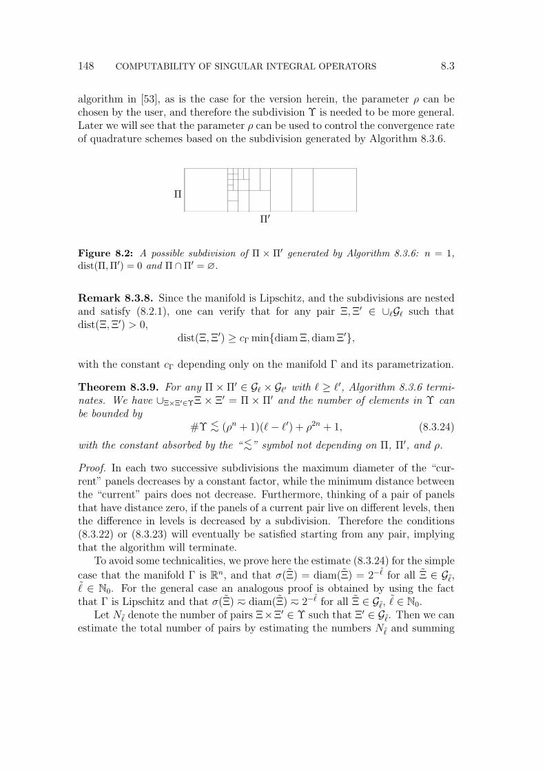
148 COMPUTABILITY OF SINGULAR INTEGRAL OPERATORS 8.3
algorithm in [53], as is the case for the version herein, the parameter ρ can bechosen by the user, and therefore the subdivision Υ is needed to be more general.Later we will see that the parameter ρ can be used to control the convergence rateof quadrature schemes based on the subdivision generated by Algorithm 8.3.6.
4 Computability 16
2. If the pair ! and !! does satisfy one of the conditions
dist(!, !!) ! ! · max"(!),"(!!), (4.22)
ordist(!, !!) = 0 and ! = ", !! " G!, (4.23)
accept the pair: # := # # !$ !!. If not, go to either step 3 or 4.
3. If #! % #, subdivide !! into next level elements !!i " G!!+1, and perform step 2 with#! = #! + 1, !! = !!i for each !!i.
4. If #! > #, subdivide ! into next level elements !i " G!+1, and perform step 2 with# = # + 1, ! = !i for each !i.
Remark 4.8. Algorithm 4.7 can already be found in, e.g., [Har01, LS99, vPS97] with "(!) =2"! for ! " G!. This nonuniform subdivision e$ectively distributes the “strength” of thenearly singular behavior of the integrand over individual subdomains. In [LS99, vPS97] thevalue of ! is fixed independent of the user and the subdivision # is of type # = !$#!, where#! is a subdivision of !!. For the algorithm in [Har01], as is the case for the version herein,the parameter ! can be chosen by the user, and therefore the subdivision # is needed to bemore general. Later we will see that the parameter ! can be used to control the convergencerate of quadrature schemes based on the subdivision generated by Algorithm 4.7.
"
"!
Fig. 2: A possible subdivision of "$"! generated by Algorithm 4.7: n = 1, dist(", "!) = 0and " &"! = '.
Remark 4.9. Since the manifold is Lipschitz, and the subdivisions are nested and satisfy (3.1),one can verify that for any pair !, !! " #!G! such that dist(!, !!) > 0,
dist(!, !!) ! c! mindiam!, diam!!,
with the constant c! depending only on the manifold % and its parametrization.
Theorem 4.10. For any "$ "! " G! $ G!! with # ! #!, Algorithm 4.7 terminates. We have#"#"!$#!$ !! = "$"! and the number of elements in # can be bounded by
## <( (!n + 1)(#) #!) + !2n + 1, (4.24)
with the constant absorbed by the “<(” symbol not depending on ", "!, and !.
Proof. In each two successive subdivisions the maximum diameter of the “current” panelsdecreases by a constant factor, while the minimum distance between the “current” pairs doesnot decrease. Furthermore, thinking of a pair of panels that have distance zero, if the panels ofa current pair live on di$erent levels, then the di$erence in levels is decreased by a subdivision.
Figure 8.2: A possible subdivision of Π × Π′ generated by Algorithm 8.3.6: n = 1,dist(Π,Π′) = 0 and Π ∩Π′ = ∅.
Remark 8.3.8. Since the manifold is Lipschitz, and the subdivisions are nestedand satisfy (8.2.1), one can verify that for any pair Ξ,Ξ′ ∈ ∪`G` such thatdist(Ξ,Ξ′) > 0,
dist(Ξ,Ξ′) ≥ cΓ mindiam Ξ, diam Ξ′,
with the constant cΓ depending only on the manifold Γ and its parametrization.
Theorem 8.3.9. For any Π× Π′ ∈ G` × G`′ with ` ≥ `′, Algorithm 8.3.6 termi-nates. We have ∪Ξ×Ξ′∈ΥΞ × Ξ′ = Π × Π′ and the number of elements in Υ canbe bounded by
#Υ <∼ (ρn + 1)(`− `′) + ρ2n + 1, (8.3.24)
with the constant absorbed by the “<∼” symbol not depending on Π, Π′, and ρ.
Proof. In each two successive subdivisions the maximum diameter of the “cur-rent” panels decreases by a constant factor, while the minimum distance betweenthe “current” pairs does not decrease. Furthermore, thinking of a pair of panelsthat have distance zero, if the panels of a current pair live on different levels, thenthe difference in levels is decreased by a subdivision. Therefore the conditions(8.3.22) or (8.3.23) will eventually be satisfied starting from any pair, implyingthat the algorithm will terminate.
To avoid some technicalities, we prove here the estimate (8.3.24) for the simple
case that the manifold Γ is Rn, and that σ(Ξ) = diam(Ξ) = 2−˜for all Ξ ∈ G˜,
˜ ∈ N0. For the general case an analogous proof is obtained by using the factthat Γ is Lipschitz and that σ(Ξ) h diam(Ξ) h 2−
˜for all Ξ ∈ G˜, ˜∈ N0.
Let N˜ denote the number of pairs Ξ×Ξ′ ∈ Υ such that Ξ′ ∈ G˜. Then we canestimate the total number of pairs by estimating the numbers N˜ and summing

8.3 COMPUTABILITY 149
over all ˜. It is obvious that if dist(Π,Π′) > 0, the number of pairs Ξ×Ξ′ ∈ Υ thatsatisfy (8.3.23) is zero, and if dist(Π,Π′) = 0, this number is uniformly bounded.Since in (8.3.24) this number is absorbed by the term 1 at the right hand side, inthe remainder we will only count pairs of type (8.3.22).
In case ˜≤ `, we have Ξ = Π for any Ξ′ ∈ G˜ with Ξ×Ξ′ ∈ Υ. When, moreover˜ > `′ we have dist(Π,Ξ′) ≤ (2ρ + 2)2−
˜. Indeed, if not, then the “parent”
Ξ′′ ∈ G˜−1 of Ξ′ would have satisfied dist(Π,Ξ′′) > 2ρ2−˜
= maxσ(Π), σ(Ξ′′)and so Ξ′ would never have been created by the algorithm. We conclude that for
`′ < ˜≤ `, N˜<∼((2ρ+ 2)2−
˜+ 2−`
)n/2−
˜n <∼ ρn + 1.
Now we consider Ξ × Ξ′ ∈ Υ with Ξ′ ∈ G˜ and ˜> ` (and such that Ξ × Ξ′
satisfies (8.3.22)). By construction of the algorithm, we have either Ξ ∈ G˜ orΞ ∈ G˜−1. Similar arguments as have been used above show that for fixed Ξ,the number of such pairs is bounded by a constant multiple of ρn + 1. Since thenumber of such Ξ is bounded by a constant multiple of 2(˜−`)n, we conclude thatfor ˜> `, N˜
<∼ (ρn + 1)2(˜−`)n.In light of Remark 8.3.8, it is easy to see that the smallest subelements gener-
ated by this algorithm will belong to the level `max with ρ2−`max >∼ 2−`, implyingthat 2(`max−`)n <∼ ρn. Therefore, we conclude that the number of elements in thesubdivision Υ is bounded by a constant multiple of
1 +`max∑
˜=`′+1
N˜<∼ 1 +
∑˜=`′+1
(ρn + 1) +`max∑
˜=`+1
(ρn + 1)2(˜−`)n
<∼ (ρn + 1)(`− `′) + ρ2n + 1.
From the condition (8.3.23), we have that the singular integrals correspondingto the subdivision Υ are always over pairs of panels on the same level. In thispaper, we make the following Assumption 8.3.10 on quadrature schemes for com-puting those singular integrals. For completeness, in Section 8.4 we confirm thisassumption for the simple case of the single layer kernel on polyhedral surfaces inR3. In any case for weakly- and strongly singular integrals, using the quadratureschemes from e.g. [72, 74], we expect that Assumption 8.3.10 can be verifiedgenerally.
Assumption 8.3.10. We assume that there exist d∗0 ∈ R and %0 > 1 such thatfor any λ, λ′ ∈ Λ with |λ| ≥ |λ′|, Ξ,Ξ′ ∈ G|λ| with dist(Ξ,Ξ′) = 0, and for anyorder p ∈ N, an approximation I∗λλ′(Ξ,Ξ
′) of Iλλ′(Ξ,Ξ′) can be computed within
W <∼ p2n arithmetical operations, having an error
|Iλλ′(Ξ,Ξ′)− I∗λλ′(Ξ,Ξ)′| <∼ %−p0 2||λ|−|λ′||d∗0 . (8.3.25)

150 COMPUTABILITY OF SINGULAR INTEGRAL OPERATORS 8.3
Now we are ready to present an algorithm how to compute the integral (8.3.11)with the help of a generally non-uniform subdivision of the integration domainΠ× Π′.
Algorithm 8.3.11 Computation of the integral Iλλ′(Π,Π′)
Parameters: Let Ψ be of P -type of order e, and let p ∈ N and ρ > 1 be given.Choose the function σ(·) as in Lemma 8.3.4.
Input: λ, λ′ ∈ Λ, and Π ∈ Gλ, and Π′ ∈ Gλ′ .Output: I∗λλ′(Π,Π
′) ∈ R.1: Apply Algorithm 8.3.6 with the above ρ and σ(·) to get the subdivision Υ of
Π× Π′;2: For each subdomain Ξ×Ξ′ ∈ Υ apply either step 4 or 5; and sum the results
as in (8.3.11), to get I∗λλ′(Π,Π′);
3: If dist(Ξ,Ξ′) > 0, apply the quadrature scheme of order p from Lemma 8.3.4;4: If dist(Ξ,Ξ′) = 0, apply the computational scheme of order p from Assump-
tion 8.3.10.
Remark 8.3.12. For Q-type wavelets, Algorithm 8.3.11 can be redefined by re-placing ”Lemma 8.3.4” by ”Lemma 8.3.5”.
Theorem 8.3.13. Let Ψ be of P -type of order e, and assume that an approxi-mation I∗λλ′(Π,Π
′) of Iλλ′(Π,Π′) is computed by using Algorithm 8.3.11. Assume
that n ≥ 2t. Then, in case that
dist(Π,Π′) ≥ ρmaxσ(Π), σ(Π′), (8.3.26)
with e∗ = e− 1− 2t− n, the error of the numerical integration satisfies
|Eλλ′(Π,Π′)| <∼ ρ−p2−||λ|−|λ′||(t+n/2)
(dist(Π,Π′)
ρmaxσ(Π), σ(Π′)
)e∗−p, (8.3.27)
and the work for computing I∗λλ′(Π,Π′) is bounded by a constant multiple of p2n,
provided that p ≥ maxe− 1, e∗ + 1. In case that (8.3.26) does not hold, for anyd∗1 ≥ |t| − n/2, with d∗1 > −n/2 when t = 0, the error satisfies
|Eλλ′(Π,Π′)| <∼ ρ−p2||λ|−|λ′||d∗1 + %−p0 2||λ|−|λ
′||d∗0 , (8.3.28)
and the work is bounded by a constant multiple of p2n(1 + ||λ| − |λ′||), providedthat p ≥ maxe− 1, e∗ +1. In view of Remark 8.3.12, these results also hold forQ-type wavelets of order e.
By taking % := min%0, ρ and d∗ := maxd∗0, d∗1, we conclude that the criteria(8.3.5) and (8.3.6) for s∗-computability from Theorem 8.3.2 are satisfied.

8.3 COMPUTABILITY 151
Proof. Without loss of generality, we assume that |λ| ≥ |λ′|. First, we willconsider the case that (8.3.26) holds. In this case, we have the subdivision Υ =Π × Π′, and so the computational work is of order of p2n. Applying Lemma8.3.4 with Θ = κ−1(Π) and Θ′ = κ−1(Π′), taking into account the definition of ω,and using the fact that ω ≥ ρ > 1 and that minσ(Π), σ(Π′) <∼ 2−|λ|, we get
|Eλλ′(Π,Π′)| <∼ 2(|λ|−|λ′|)(n/2−t)ω−(n+p) max1, ωe−1 minσ(Π), σ(Π′)n
× dist(Π,Π′)−2t
<∼ 2−|λ|(t+n/2)+|λ′|(t−n/2)ωe−1−n−pω−2t maxσ(Π), σ(Π′)−2t.
Now using the estimate maxσ(Π), σ(Π′) h 2−|λ′| and n ≥ 2t, we have
|Eλλ′(Π,Π′)| . 2−(|λ|−|λ′|)(t+n/2)−|λ′|(n−2t)ωe∗−p
. ρ−p2−(|λ|−|λ′|)(t+n/2)(ω/ρ)e∗−p,
proving the first part of the theorem.
Let us now consider the case that (8.3.26) does not hold. Since ρ is fixed, thenumber of subdomains of the subdivision Υ is of order 1 + ||λ| − |λ′||, and thuswe get the work bound. By Assumption 8.3.10, the sum of the errors made in theapproximations for Iλλ′(Ξ,Ξ
′) with Ξ× Ξ′ ∈ Υ and dist(Ξ,Ξ′) = 0 is responsiblefor the last term in (8.3.28).
We need to estimate the portion of the total error Eλλ′(Π,Π′) that corresponds
to the integrals Iλλ′(Ξ,Ξ′) with Ξ × Ξ′ ∈ Υ and dist(Ξ,Ξ′) > 0. We denote by
I1 the sum of all these integrals arising from the subdivision Υ, and by I∗1 thecomputed approximation for I1. Since by construction for any Ξ × Ξ′ ∈ Υ withdist(Ξ,Ξ′) > 0 it holds that dist(Ξ,Ξ′)
maxσ(Ξ),σ(Ξ′) ≥ ρ > 1, Lemma 8.3.4 gives
|I1 − I∗1 | .∑
Ξ×Ξ′∈Υ:dist(Ξ,Ξ′)>0
2(|λ|−|λ′|)(n/2−t)ρe−1−n−p (8.3.29)
×minσ(Ξ), σ(Ξ′)n dist(Ξ,Ξ′)−2t
. ρ−p2−|λ|(t+n/2)+|λ′|(t−n/2)
∑Ξ×Ξ′∈Υ:dist(Ξ,Ξ′)>0
dist(Ξ,Ξ′)−2t,
where we have used that minσ(Ξ), σ(Ξ′) <∼ 2−|λ|.
From the proof of Lemma 8.3.9, recall that for the number N˜ of Ξ× Ξ′ ∈ Υwith Ξ′ ∈ G˜, we have N˜ = 0 for ˜ > `max where, since ρ is a fixed constant,
`max − |λ| <∼ 1, and furthermore N˜<∼ 1 for |λ′| ≤ ˜≤ `max. Since for Ξ× Ξ′ ∈ Υ
with dist(Ξ,Ξ′) > 0 and Ξ′ ∈ G˜, dist(Ξ,Ξ′) h 2−˜, we may bound the sum in the

152 COMPUTABILITY OF SINGULAR INTEGRAL OPERATORS 8.4
last row of (8.3.29) on a constant multiple of
`max∑˜=|λ′|
2˜·2t <∼
1 + ||λ| − |λ′|| if t = 0,
2|λ′|·2t if t < 0,
2|λ|·2t if t > 0.
By substituting this result into (8.3.29), the proof is completed.
8.4 Quadrature for singular integralsIn this section, we confirm Assumption 8.3.10 for the simple case of the singlelayer kernel on polyhedral surfaces in R3.
We assume that the manifold Γ is the surface of a three dimensional polyhe-dron, and that the subdivisions G`, (` ∈ N), are generated by dyadic refinementsof G0, being an initial conforming triangulation of Γ.
We take the operator L to be the single layer operator (thus t = −12) having
the kernel
K(z, z′) =1
4π|z − z′|z 6= z′, (8.4.1)
and assume that the wavelet basis Ψ is of P -type of order e. Let λ, λ′ ∈ Λ beindices with |λ| ≥ |λ′|. Then in view of Assumption 8.3.10, we are ultimatelyinterested in computing the integral
I :=
∫Ξ
∫Ξ′K(z, z′)ψλ(z)ψλ′(z
′)dΓzdΓz′ , (8.4.2)
where Ξ,Ξ′ ∈ G|λ| and dist(Ξ,Ξ′) = 0. With
T := (x1, x2) ∈ R2 : 0 < x2 < x1 < 1,
we can find affine bijections χΞ : T → Ξ, and χΞ′ : T → Ξ′, thus with JacobiansJΞ := |∂χΞ| h 2−2|λ|, and JΞ′ := |∂χΞ′| h 2−2|λ|, such that
I =
∫T
∫T
g(x, y)
|r(x, y)|dxdy, (8.4.3)
where g(x, y) := (4π)−1JΞJΞ′ψλ(χΞ(x))ψλ′(χΞ′(y)) and r(x, y) := χΞ′(y)− χΞ(x).Taking into account that n = 2 and t = −1
2, from (8.2.2) we derive the following
estimates for β ∈ N20
|∂βxg| <∼ 2−52|λ|+ 3
2|λ′| and |∂βy g| <∼ 2−
52|λ|+ 3
2|λ′|2(|λ′|−|λ|)|β|. (8.4.4)

8.4 QUADRATURE FOR SINGULAR INTEGRALS 153
We present here a slight variation of the quadrature scheme developed in e.g.[67, 72, 74], see also [73]. The idea is to apply a degenerate coordinate transfor-mation which is a generalization of the so called Duffy’s triangular coordinates,effectively removing the singularity of the integrand while preserving a polyhe-dral shape of the integration domain. The coordinate transformations introducedhere are somewhat simpler than the ones in the above mentioned papers, and weexpect that the presentation is geometrically more intuitive.
To this end, we need to partition the integration domain T×T into severalpyramides, which is necessary for us to use Duffy’s transformations in order toremove the singularities, cf. [67, 72]. Denote the vertices of the triangle T byA0 = (0, 0), A1 = (0, 1), and A2 = (1, 1). Then obviously, T×T has nine verticesAik := Ai × Ak for i, k = 0, 1, 2. Note that A00 = O.
We break T×T up into two pyramides D1 := (x, y) ∈ T×T : x1 > y1 andD2 := (x, y) ∈ T×T : x1 < y1. One can verify that D1 is the pyramid withvertex O and base B1 = A10A11A12A20A21A22, being a triangular prism, andthat D2 is the pyramid with vertex O and base B2 B2 = A01A11A21A02A12A22,being also a triangular prism. Moreover, these prisms can be described as B1 =1× (0, 1)×T and B2 = T ×1× (0, 1). Introducing the reflection with respectto the plane x = y by R : (x, y) 7→ (y, x), we notice the symmetry B2 = RB1
and so D2 = RD1.By subdividing the prism B1 into tetrahedra, we can get a simplicial parti-
tioning of T×T , because any simplicial partitioning of B1 induces a simplicialpartitioning of D1, and by taking the image under the mapping R, a simplicialpartitioning of D2. Our choice of such a partitioning is depicted in Figure 8.3.
A20
A21
A22
A10
A11
A12
Figure 8.3: A simplicial partitioning of the prism B1.
Consequently, the domain T×T is subdivided into the following simplices

154 COMPUTABILITY OF SINGULAR INTEGRAL OPERATORS 8.4
described by their vertices.
D1
S1 = OA10A11A12A22,S2 = OA10A11A20A22,S3 = OA11A20A21A22,
and D2
S4 = OA01A11A21A22,S5 = OA01A11A02A22,S6 = OA11A02A12A22.
We notice the symmetry Si = RSi+3 for i = 1, 2, 3. The above partitioningsof T×T will be used in quadrature schemes for the integral (8.4.3).
In the following we will distinguish three basic cases:
• Coincident panels: Ξ = Ξ′, that is, the case of identical panels;
• Edge adjacent panels: Ξ and Ξ′ share one common edge;
• Vertex adjacent panels: Ξ and Ξ′ share one common vertex.
In view of (8.4.3), we need to integrate a singular function over a four dimen-sional polyhedral domain T × T . The singularity of the function is located ondifferent dimensional sets in different situations: whereas the singularity occursat a point for vertex adjacent integrals, it occurs all along an edge in case theintegral is edge adjacent, and for coincident integrals, the singularity is on a twodimensional “diagonal” of the domain. Therefore in each of the three cases, wefirst characterize the singularity in terms of the distance to the singularity set, andthen introduce special coordinate transformations that annihilate the singularity.
Case of identical panels
First we will discuss the case of identical panels Ξ = Ξ′. In this case, the differencer = χΞ(y)− χΞ(x) is zero if and only if t := y − x = 0. Since χΞ is affine, we canwrite
r = 2−|λ|l1(t) = 2−|λ|l1(y1 − x1, y2 − x2),
where l1 : R2 7→ R3 is a linear function depending only on the shape of Ξ. Notingthat any panel Ξ is similar to a panel from the initial triangulation, we only haveto deal with finitely many functions l1. Introducing polar coordinates (ρ, θ) in R2
by ρ = |t| and θ = t/|t| ∈ S1, being the unit circle in R2, this difference r readsas
r = 2−|λ|ρl1(θ).
Our goal is now to obtain an expression for |r|−1, because this quantity essentiallydetermines the singular behavior of the local kernel. Since r is defined on some

8.4 QUADRATURE FOR SINGULAR INTEGRALS 155
complete neighborhood of t = 0, the function l1(θ) has to be nonzero for anyθ ∈ S1, and so we have
|r|−1 = 2|λ|ρ−1a(θ)
with a(θ) := |l1(θ)|−1 which is analytic in a neighborhood of S1. Now the inte-grand of (8.4.3) can be written as
|r(x, y)|−1g(x, y) = 2|λ|ρ−1a(θ)g(x, y). (8.4.5)
It is time to use the above described simplicial partitioning of the integrationdomain T × T , in combination with special coordinate transformations for thepurpose of removing the singularity of the integrand. Introducing the notationP := T×(0, 1)×(0, 1), we define the transformations φi : P→Si : (η, ζ, ξ) 7→ (x, y)for i ∈ 1, 6.
φ1(η, ζ, ξ) =
(1− ξ)η1 + ξ
(1− ξ)η2
(1− ξ)η1 + ξζ(1− ξ)η2 + ξζ
, φ2(η, ζ, ξ) =
(1− ξ)η1 + ξ(1− ξ)η2 + ξζ
(1− ξ)η1
(1− ξ)η2
,
φ3(η, ζ, ξ) =
(1− ξ)η1 + ξ(1− ξ)η2 + ξ(1− ξ)η1 + ξζ
(1− ξ)η2
, (8.4.6)
and φi+3 := Rφi for i = 1, 2, 3. The Jacobian of each transformation φi is givenby ξ(1−ξ)2. Recall that ρ−1 characterizes the singularity of the integrand (8.4.5).In this regard, for each transformation φi one can show that
ρ = ξfi(ζ), with an analytic fi(ζ)≥ 1√2
for any ζ ∈ [0, 1].
For instance, for φ1 we have
ρ2 = ξ2(ζ2 + (1− ζ)2) ≥ ξ2·12,
since ζ2 + (1 − ζ)2≥12
for any ζ ∈ R. Moreover, for each φi one can verify thatθ = ϑi(ζ) for some analytic function ϑi : [0, 1] → S1.
In all, the Jacobian of the mapping φi annihilates the singularity in the inte-grand (8.4.5), meaning that the integral I in (8.4.3) now can be written as thefollowing proper integral
I =
∫ 1
0
∫ 1
0
∫T
ξ(1− ξ)2
6∑i=1
g(φi(η, ζ, ξ))
|r(φi(η, ζ, ξ))|dηdζdξ
= 2|λ|∫ 1
0
∫ 1
0
∫T
(1− ξ)2
6∑i=1
a(ϑi(ζ))g(φi(η, ζ, ξ))
fi(ζ)dηdζdξ.
(8.4.7)

156 COMPUTABILITY OF SINGULAR INTEGRAL OPERATORS 8.4
Therefore we will be able to use standard quadrature schemes to approximate theintegral I. Note that in numerical quadrature we can use the first expression in(8.4.7) for the integral I. The functions fi and a ϑi are introduced here merelyfor the analysis purpose.
Since the integrand in (8.4.7) is polynomial with respect to the variables ξand η, we can always choose exact quadrature rules for integrations over thosevariables.
Proposition 8.4.1. Approximate the integral (8.4.7) by a product quadraturerule Qξ×Qζ×Qη, where Qξ and Qη are quadrature rules exact for the integrationover the variables ξ ∈ (0, 1) and η ∈ T , respectively, and Qζ is a compositequadrature rule for the integration over ζ ∈ (0, 1) of varying order p and fixedrank N . Then there exist a constant δ > 0 such that the quadrature error satisfies
|E(Ξ,Ξ′)| <∼ 2−32(|λ|−|λ′|)(δN)−p. (8.4.8)
Choosing N such that δN > 1, we conclude that in this case Assumption 8.3.10is fulfilled with d∗0 = −3
2.
Proof. In view of Lemma 7.2.4, it suffices to consider the integration over ζ. Usingthe analyticity of ζ 7→ a(ϑi(ζ))
fi(ζ)one derives
supζ∈[0,1]
∣∣∣∣∂kζ a(ϑi(ζ))fi(ζ)
∣∣∣∣ <∼ k!
δkfor k ∈ N0, i ∈ 1, 6,
for some constant δ > 0. From (8.4.4) and (8.4.6) we have for each i ∈ 1, 6 thatg φi is a polynomial of order e and
|∂kζ (g φi)| <∼ 2−52|λ|+ 3
2|λ′| for k ∈ 1, e− 1.
Now using Proposition 7.2.6 the proof is obtained.
Case of edge adjacent panels
Now we will discuss the case when Ξ and Ξ′ share exactly one common edge.Without loss of generality, we assume that χΞ(x) = χΞ′(x) for all x ∈ (0, 1)×0.Then, the difference r = χΞ′(y)− χΞ(x) is zero if and only if
t = (t1, t2, t3) := (y1 − x1, x2, y2)
equals zero. Since χΞ and χΞ′ are affine, we can write
r = χΞ′(x1 + t1, t3)− χΞ(x1, t2) = 2−|λ|l1(t),

8.4 QUADRATURE FOR SINGULAR INTEGRALS 157
where l1 : R3 → R3 is a linear function depending only on the shapes of Ξ andΞ′. Introducing polar coordinates (ρ, θ) in R3 by ρ = |t| and θ = t/|t| ∈ S2, beingthe unit sphere in R3, this difference r reads as
r = r(ρ, θ) = 2−|λ|ρl1(θ).
Since r is defined on a complete neighborhood of t = 0 in R× R2≥0, the function
l1(θ) 6= 0 for any θ ∈ S2 with θ2, θ3 ≥ 0, allowing us to write
|r|−1 = 2|λ|ρ−1b(θ)
with b(θ) := |l1(θ)|−1 which is analytic in a neighborhood of S2 ∩(R× R2
≥0
).
Then the integrand of (8.4.3) can be written as
|r(x, y)|−1g(x, y) = 2|λ|ρ−1b(θ)g(x, y). (8.4.9)
Now we define the transformations φi : P→Si : (η, ζ, ξ) 7→ (x, y) for i ∈ 1, 6.
φ1(η, ζ, ξ) =
(1− ξ)ζ + ξ
ξη2
(1− ξ)ζ + ξη1
ξη1
, φ2(η, ζ, ξ) =
(1− ξ)ζ + ξ
ξη1
(1− ξ)ζ + ξη2
ξη2
,
φ3(η, ζ, ξ) =
(1− ξ)ζ + ξ
ξ(1− ξ)ζ + ξη1
ξη2
, (8.4.10)
and φi+3 := R φi for i = 1, 2, 3. For each transformation φi one can show thatthe Jacobian equals ξ2(1− ξ), and that
ρ = ξfi(η), with an analytic fi(η)≥ 1√2
for any η ∈ T .
For instance, for φ1 we have
ρ2 = ξ2(η21 + (1− η1)
2 + η22) ≥ ξ2·1
2.
Moreover, for each φi one can verify that θ = ϑi(η) with some analytic functionϑi : T → S2.
In all, the Jacobian of the mapping φi annihilates the singularity in the inte-grand (8.4.9), meaning that the integral I in (8.4.3) now can be written as the

158 COMPUTABILITY OF SINGULAR INTEGRAL OPERATORS 8.4
following proper integral
I =
∫ 1
0
∫ 1
0
∫T
ξ2(1− ξ)6∑i=1
g(φi(η, ζ, ξ))
|r(φi(η, ζ, ξ))|dηdζdξ
= 2|λ|∫ 1
0
∫ 1
0
∫T
ξ(1− ξ)6∑i=1
b(ϑi(η))g(φi(η, ζ, ξ))
fi(η)dηdζdξ,
(8.4.11)
and thus the standard quadrature schemes on P can be applied.
Proposition 8.4.2. Approximate the integral (8.4.11) by a product quadraturerule Qξ×Qζ×Qη, where Qξ and Qζ are quadrature rules exact for the integrationover the variables ξ, ζ ∈ (0, 1), respectively, and Qη is a composite quadrature rulefor the integration over η ∈ T of varying order p and fixed rank N . Then thereexist a constant δ > 0 such that the quadrature error satisfies
|E(Ξ,Ξ′)| <∼ 2−32(|λ|−|λ′|)(δN)−p. (8.4.12)
Choosing N such that δN > 1, we conclude that in this case Assumption 8.3.10is fulfilled with d∗0 = −3
2.
The proof is obtained similarly to the proof of Proposition 8.4.1.
Case of vertex adjacent panels
Let Ξ and Ξ′ share exactly one common point. Without loss of generality, weassume that χΞ(0) = Ξ∩Ξ′ = χΞ′(0). Then obviously, the difference r = r(x, y) =χΞ′(y)− χΞ(x) is zero if and only if t := (x, y) equals zero. Since χΞ and χΞ′ areaffine, we can write
r(x, y) = 2−|λ|l1(x, y),
where l1 : R4 → R3 is a linear function depending only on the shapes of Ξ andΞ′. Introducing polar coordinates (ρ, θ) in R4 by ρ = |t| and θ = t/|t| ∈ S3, beingthe unit sphere in R4, this difference r reads as
r = r(ρ, θ) = 2−|λ|ρl1(θ).
Since r is defined on a complete neighborhood of t = 0 in t ∈ R4 : t1 ≥ t2 ≥0, t3 ≥ t4 ≥ 0, the function l1(θ) 6= 0 for any θ ∈ S3 with θ1 ≥ θ2 ≥ 0 andθ3 ≥ θ4 ≥ 0, allowing us to write
|r|−1 = 2|λ|ρ−1c(θ)

8.4 QUADRATURE FOR SINGULAR INTEGRALS 159
with c(θ) := |l1(θ)|−1 which is analytic in a neighborhood of θ ∈ S3 : θ1 ≥ θ2 ≥0, θ3 ≥ θ4 ≥ 0. Then the integrand of (8.4.3) can be written as
|r(x, y)|−1g(x, y) = 2|λ|ρ−1c(θ)g(x, y). (8.4.13)
We define the transformations φ1 and φ2 that map the coordinates (η, ζ, ξ)∈ P onto the four dimensional pyramides D1 and D2 respectively.
φ1(η, ζ, ξ) = ξ(1, ζ, η1, η2), and φ2(η, ζ, ξ) = ξ(η1, η2, 1, ζ). (8.4.14)
Notice that φ1 = R φ2 with R being the reflection x↔y. For both of thetransformations, the Jacobian equals ξ3, and we have
ρ = ξf(η, ζ) with f(η, ζ) =√
1 + η12 + η2
2 + ζ2.
Moreover, we have θ = ϑ1(η, ζ) := f(η, ζ)−1(1, ζ, η1, η2) for the transformationφ1, and θ = ϑ2(η, ζ) := Rϑ1(η, ζ) for the transformation φ2.
In all, the Jacobian of the mapping φi annihilates the singularity in the inte-grand (8.4.13), meaning that the integral I in (8.4.3) now can be written as thefollowing proper integral
I =
∫ 1
0
∫ 1
0
∫T
ξ3
2∑i=1
g(φi(η, ζ, ξ))
|r(φi(η, ζ, ξ))|dηdζdξ
= 2|λ|∫ 1
0
∫ h
0
∫T
ξ2
2∑i=1
c(ϑi(η, ζ))g(φi(η, ζ, ξ))
f(η, ξ)dηdζdξ,
(8.4.15)
and thus the standard quadrature schemes on P can be applied.
Proposition 8.4.3. Approximate the integral (8.4.15) by a product quadraturerule Qξ × Qζ × Qη, where Qξ is a quadrature rule exact for the integration overξ ∈ (0, 1), and Qζ and Qη are composite quadrature rules for the integration overζ ∈ (0, 1) and η ∈ T , respectively, of varying order p and fixed rank N . Thenthere exist a constant δ > 0 such that the quadrature error satisfies
|E(Ξ,Ξ′)| <∼ 2−32(|λ|−|λ′|)(δN)−p. (8.4.16)
Choosing N such that δN > 1, we conclude that in this case Assumption 8.3.10is fulfilled with d∗0 = −3
2.

160 COMPUTABILITY OF SINGULAR INTEGRAL OPERATORS 8.4

Chapter 9Conclusion
9.1 DiscussionIn [17, 18], Cohen, Dahmen and DeVore introduced adaptive wavelet paradigmsfor solving operator equations. A number of algorithms with asymptotically opti-mal computational complexity were developed, among others, under the assump-tion that on average, an individual entry of the stiffness matrix can be computedat unit cost. Although it has been indicated that this assumption is realistic, itis far from obvious.
The work presented in this thesis shows that the average unit cost assumptionis valid for both differential and singular integral operators, at least when thewavalets are piecewise polynomials (Chapters 7 and 8). As a consequence, wecan conclude that the “fully discrete” adaptive wavelet algorithm has optimalcomputational complexity.
A crucial ingredient for proving the optimal complexity of the adaptive waveletalgorithms was the coarsening step that was applied after every fixed numberof iterations. As we have shown in Chapter 3, it turns out that coarsening isunnecessary for proving optimal computational complexity of algorithms of thetype considered in [17]. Since with the new method no information is deleted thathas been created by a sequence of computations, we expect that it is more efficient.The algorithm from Chapter 3 can be applied directly with minor modificationsto a larger class of problems (Chapter 5). We also investigated the possibilityof using polynomial preconditioners in the context of adaptive wavelet methods(Chapter 4).
In [5, 54], adaptive wavelet methods with “truncated” residuals were intro-duced which are modifications of the methods from [17], and convincing numericalexperiments were reported showing that the methods are comparatively efficient.We developed a theoretical framework that could be used to prove optimal com-
161

162 CONCLUSION 9.2
putational complexity of the methods with truncated residuals, and for ellipticboundary value problems, a complete proof of optimality is given (Chapter 6).
9.2 Future workThere are many interesting directions in which future research on adaptive waveletalgorithms can be taken.
Proving optimality of adaptive wavelet BEMs with truncated residuals is aninteresting and important open issue. Supposing that the proof would be similarto our proof in the case of methods for boundary value problems (Chapter 6),one would need efficient and reliable a posteriori error estimators for BEMs. Toour knowledge, the only known such estimators are those developed by BirgitFaermann, cf. [42, 43, 44]. Then, the so-called local discrete lower bound forthose estimators seems to be far from obvious. This direction could also be a wayto approach the convergence and complexity analyses of adaptive BEMs.
Another interesting topic is the use of anisotropically supported wavelets foradaptive algorithms. When isotropically supported wavelets are employed, theconvergence rate grows with the regularity of the solution in terms of (isotropic)Besov spaces (cf. Chapter 2), and decreases with increasing space dimension. Thelatter fact is an instance of the so called curse of dimensionality. Fortunately,high dimensional problems are usually simple and formulated on tensor productdomains, and this exceptionally symmetric structure seems to give rise to a cer-tain regular behaviour of the solution. Recently, Nitsche [65] identified certainanisotropic Besov spaces as the natural smoothness spaces for measuring the reg-ularity of the solution when anisotropically supported tensor product wavelets areemployed. It is also shown that in two and three dimensions, solutions to ellip-tic PDE’s exhibit arbitrarily high regularity measured in terms of these spaces,while it is not known whether the same holds in the isotropic setting. More-over, adaptive wavelet algorithms applied with anisotropically supported tensorproduct wavelets are proven to display asymptotically optimal convergence ratesindependent of space dimension, only restricted by the anisotropic Besov regular-ity of the solution and certain properties of the wavelets which can be bettered atwill by choosing appropriate wavelets, cf. [65, 79]. So above all, it seems that thecurse of dimensionality can be avoided. Yet, there still remains a few technicaldetails. One has to be sure that the constants in the asymptotic estimates donot blow up with increasing dimension. Although it is generally expected, a suf-ficient regularity of the PDE’s in more than three dimension needs to be verified.Furthermore, appropriate data structures for the implementation of the adaptivewavelet methods for high dimensions should be identified.
Anisotropically supported wavelets could also pay off even in low dimensions

9.2 FUTURE WORK 163
when a strong singularity along a layer is present, for instance, when boundary in-tegral equations on polyhedra, or singularly perturbed boundary value problemsare considered. There have appeared some interesting results in the directionof using (isotropic as well as anisotropic) wavelets for stabilizing singularly per-turbed boundary value problems, cf. [6, 13].
Furthermore, there are many related active research areas that are not touchedupon in this thesis. Those include the issues of adaptive wavelet methods fornonlinear variational problems (cf. [3, 19, 20, 35]), using wavelets for goal orientedadaptivity (cf. [31]), using wavelet frames instead of a basis (cf. [27, 28, 83]), andadaptive wavelet methods for eigenvalue computation.

164 CONCLUSION

Bibliography
[1] S. F. Ashby, T. A. Manteuffel, and J. S. Otto, A comparison ofadaptive Chebyshev and least squares polynomial preconditioning for Her-mitian positive definite linear systems, SIAM J. Sci. Statist. Comput., 13(1992), pp. 1–29.
[2] K. Atkinson, The numerical solution of boundary integral equations, inThe State of the Art in Numerical Analysis, I. Duff and G. Watson, eds.,Clarendon Press, Oxford, 1997, pp. 223–259.
[3] A. Barinka, Fast computation tools for adaptive wavelet schemes, PhDthesis, RWTH Aachen, Germany, March 2005.
[4] J. Bergh and J. Lofstrom, Interpolation spaces: An introduction,vol. 223 of Grundlehren der mathematischen Wissenschaften, Springer-Verlag, Berlin, Heidelberg, New York, 1976.
[5] S. Berrone and T. Kozubek, An adaptive WEM algorithm for solvingelliptic boundary problems in fairly general domains, Preprint 38, Politecnicodi Torino, Italy, 2004. Submitted.
[6] S. Bertoluzza, C. Canuto, and A. Tabacco, Stable discretizations ofconvection-diffusion problems via computable negative-order inner products,SIAM J. Numer. Anal., 38 (2000), pp. 1034–1055 (electronic).
[7] G. Beylkin, R. Coifman, and V. Rokhlin, The fast wavelet transformand numerical algorithms, Comm. Pure & Appl. Math., 44 (1991), pp. 141–183.
[8] P. Binev, W. Dahmen, and R. DeVore, Adaptive finite element methodswith convergence rates, Numer. Math., 97(2) (2004), pp. 219–268.
165
166 BIBLIOGRAPHY
[9] K. Bittner and K. Urban, Adaptive wavelet methods using semiorthogo-nal spline wavelets: Sparse evaluation of nonlinear functions, preprint, Uni-versitat Ulm, Germany, 2004.
[10] J. Bramble and J. Pasciak, A preconditioning technique for indef-inite systems resulting from mixed approximations of elliptic problems,Math. Comp., 50(181) (1988), pp. 1–17.
[11] S. C. Brenner and R. L. Scott, The mathematical theory of finite ele-ment methods, Springer Verlag, New York, 1994.
[12] V. I. Burenkov, Sobolev spaces on domains, Teubner Verlag, Stuttgart,Leipzig, 1998.
[13] C. Canuto and A. Tabacco, Anisotropic wavelets along vector fields andapplications to PDE’s, Arab. J. Sci. Eng. Sect. C Theme Issues, 28 (2003),pp. 89–105. Wavelet and fractal methods in science and engineering, Part I.
[14] C. Canuto, A. Tabacco, and K. Urban, The wavelet element methodpart I: Construction and analysis, Appl. Comput. Harmon. Anal., 6 (1999),pp. 1–52.
[15] C. Canuto and K. Urban, Adaptive optimization in convex Banachspaces, SIAM J. Numer. Anal., 42 (2005), pp. 2043–2075.
[16] A. Cohen, Wavelet methods in numerical analysis, in Handbook of Nu-merical Analysis. Vol. VII, P. Ciarlet and J. L. Lions, eds., North-Holland,Amsterdam, 2000, pp. 417–711.
[17] A. Cohen, W. Dahmen, and R. DeVore, Adaptive wavelet schemesfor elliptic operator equations – Convergence rates, Math. Comp., 70 (2001),pp. 27–75.
[18] , Adaptive wavelet methods II – Beyond the elliptic case, Found. Com-put. Math., 2 (2002), pp. 203–245.
[19] , Adaptive wavelet schemes for nonlinear variational problems, SIAM J.Numer. Anal., 41 (2003), pp. 1785–1823.
[20] , Sparse evaluation of compositions of functions using multiscale expan-sions, SIAM J. Math. Anal., 35(2) (2003), pp. 279–303.
[21] A. Cohen, I. Daubechies, and J. C. Feauveau, Biorthogonal basesof compactly supported wavelets, Comm. Pure & Appl. Math., 45 (1992),pp. 485–560.

BIBLIOGRAPHY 167
[22] A. Cohen and R. Masson, Wavelet adaptive method for second orderelliptic problems: Boundary conditions and domain decomposition, Numer.Math., 86 (2000), pp. 193–238.
[23] M. Costabel, Boundary integral operators on Lipschitz domains: Elemen-tary results, SIAM J. Numer. Anal., 19(3) (1988), pp. 613–626.
[24] M. Costabel and W. L. Wendland, Strong ellipticity of boundary in-tegral operators, J. Reine. Angew. Math., 372 (1986), pp. 34–63.
[25] S. Dahlke, W. Dahmen, and K. Urban, Adaptive wavelet methods forsaddle point probelms – Optimal convergence rates, SIAM J. Numer. Anal.,40 (2002), pp. 1230–1262.
[26] S. Dahlke and R. DeVore, Besov regularity for elliptic boundary valueproblems, Comm. Part. Diff. Eqs., 22(1&2) (1997), pp. 1–16.
[27] S. Dahlke, M. Fornasier, and T. Raasch, Adaptive frame methodsfor elliptic operator equations, Bericht 3, Philipps-Universitat Marburg, Ger-many, 2004.
[28] S. Dahlke, M. Fornasier, T. Raasch, R. P. Stevenson, andM. Werner, Adaptive frame methods for elliptic operator equations: Thesteepest descent approach, Technical Report 1347, Utrecht University, TheNetherlands, February 2006. Submitted.
[29] W. Dahmen, Stability of multiscale transformations, J. FourierAnal. & Appl., 2 (1996), pp. 341–361.
[30] W. Dahmen, H. Harbrecht, and R. Schneider, Adaptive methods forboundary integral equations – Complexity and convergence estimates, IGPMreport 250, RWTH Aachen, Germany, March 2005.
[31] W. Dahmen, A. Kunoth, and J. Vorloeper, Convergence of adaptivewavelet methods for goal-oriented error estimation, IGPM report, RWTHAachen, 2006. To appear in Proceedings of ENUMATH 05.
[32] W. Dahmen and R. Schneider, Wavelets with complementary bound-ary conditions – Function spaces on the cube, Results in Math., 34 (1998),pp. 255–293.
[33] , Composite wavelet bases for operator equations, Math. Comp., 68(1999), pp. 1533–1567.
168 BIBLIOGRAPHY
[34] , Wavelets on manifolds I: Construction and domain decomposition,SIAM J. Math. Anal., 31 (1999), pp. 184–230.
[35] W. Dahmen, R. Schneider, and Y. Xu, Nonlinear functionals of waveletexpansions - adaptive reconstruction and fast evaluation, Numer. Math., 86(2000), pp. 49–101.
[36] W. Dahmen and R. P. Stevenson, Element-by-element construction ofwavelets satisfying stability and moment conditions, SIAM J. Numer. Anal,37 (1999), pp. 319–352.
[37] W. A. Dahmen, H. Harbrecht, and R. Schneider, Compression tech-niques for boundary integral equations - Optimal complexity estimates, SIAMJ. Numer. Anal., 43 (2006), pp. 2251–2271.
[38] S. Dekel and D. Leviatan, The Bramble-Hilbert lemma for convex do-mains, SIAM J. Numer. Anal, 35 (2004), pp. 1203–1212.
[39] R. DeVore, Nonlinear approximation, Acta Numerica, 7 (1998), pp. 51–150.
[40] S. C. Eisenstat, H. C. Elman, and M. H. Schultz, Variational itera-tive methods for nonsymmetric systems of linear equations, SIAM J. Numer.Anal., 20(2) (1983), pp. 345–357.
[41] J. v. d. Eshof and G. L. Sleijpen, Inexact Krylov subspace methods forlinear systems, SIAM J. Matrix Anal. Appl., 26 (2004), pp. 125–153.
[42] B. Faermann, Local a-posteriori error indicators for the Galerkin dis-cretization of boundary integral equations, Numer. Math., 79 (1998), pp. 43–76.
[43] , Localization of the Aronszajn-Slobodeckij norm and application to adap-tive boundary element methods. Part I. The two-dimensional case, IMA J.Numer. Anal., 20 (2000), pp. 203–234.
[44] , Localization of the Aronszajn-Slobodeckij norm and application to adap-tive boundary element methods. Part II. The three-dimensional case, Numer.Math., 92 (2002), pp. 467–499.
[45] Ts. Gantumur, An optimal adaptive wavelet method for nonsymmetric andindefinite elliptic problems, Technical Report 1343, Utrecht University, TheNetherlands, January 2006. Submitted.

BIBLIOGRAPHY 169
[46] Ts. Gantumur, H. Harbrecht, and R. P. Stevenson, An optimaladaptive wavelet method without coarsening of the iterands, Technical Re-port 1325, Utrecht University, The Netherlands, March 2005. To appear inMath. Comp.
[47] Ts. Gantumur and R. P. Stevenson, Computation of differential op-erators in wavelet coordinates, Math. Comp., 75 (2006), pp. 697–709.
[48] , Computation of singular integral operators in wavelet coordinates,Computing, 76 (2006), pp. 77–107.
[49] G. H. Golub and M. L. Overton, The convergence of inexact Chebyshevand Richardson iterative methods for solving linear systems, Numer. Math.,53 (1988), pp. 571–593.
[50] P. Grisvard, Elliptic problems in nonsmooth domains, vol. 24 of Mono-graphs and Studies in Mathematics, Pitman, Boston, London, Melbourne,1985.
[51] W. Hackbusch, Integral equations. Theory and numerical treatment,ISNM, Birkhauser Verlag, Basel, Boston, Berlin, 1995.
[52] W. Hackbusch and S. A. Sauter, On the efficient use of the Galerkinmethod to solve Fredholm integral equations, Appl. Math., 38 (1993), pp. 301–322.
[53] H. Harbrecht, Wavelet Galerkin schemes for the boundary elementmethod in three dimensions, PhD thesis, TU Chemnitz, Germany, 2001.
[54] H. Harbrecht and R. Schneider, Adaptive wavelet Galerkin BEM, inComputational Fluid and Solid Mechanics 2003, K.-J. Bathe, ed., Elsevier,Amsterdam, Boston, 2003, pp. 1982–1986.
[55] , Biorthogonal wavelet bases for the boundary element method, Math.Nachr., 269-270 (2004), pp. 167–188.
[56] H. Harbrecht and R. P. Stevenson, Wavelets with patchwise cancella-tion properties, Technical Report 1311, Utrecht University, The Netherlands,October 2004. To appear in Math. Comp.
[57] G. Hsiao and W. Wendland, Boundary element methods: foundationand error analysis, in Encyclopedia of Computational Mechanics, E. Stein,R. de Borst, and T. J. Hughes, eds., John Wiley & Sons Ltd, New York,2004.

170 BIBLIOGRAPHY
[58] O. G. Johnson, C. A. Micchelli, and G. Paul, Polynomial precondi-tioners for conjugate gradient calculations, SIAM J. Numer. Anal., 20 (1983),pp. 362–376.
[59] Ch. Lage and Ch. Schwab, Wavelet Galerkin algorithms for boundaryintegral equations, SIAM J. Sci. Comput., 20 (1999), pp. 2195–2222.
[60] V. Maz’ya and T. Shaposhnikova, Higher regularity in the classical layerpotential theory for Lipschitz domains, Indiana Univ. Math. J, 54 (2005),pp. 99–142.
[61] W. C. McLean, Strongly elliptic systems and boundary integral equations,Cambridge University Press, Cambridge, New York, 2000.
[62] K. Mekchay and R. Nochetto, Convergence of an adaptive finite ele-ment method for general second order linear elliptic PDE, preprint, Univer-sity of Maryland, 2004.
[63] A. A. R. Metselaar, Handling wavelet expansions in numerical analysis,PhD thesis, Universiteit Twente, The Netherlands, June 2002.
[64] H. Nguyen, Finite element wavelets for solving partial differential equa-tions, PhD thesis, Utrecht University, The Netherlands, April 2005.
[65] A. Nitsche, Sparse tensor product approximation of elliptic problems, PhDthesis, ETH Zurich, Switzerland, October 2004.
[66] W. M. Patterson, Iterative methods for the solution of a linear operatorequation in Hilbert space – A survey, no. 394 in Lecture Notes in Mathemat-ics, Springer-Verlag, Berlin, Heidelberg, New York, 1974.
[67] T. v. Petersdorff and Ch. Schwab, Fully discrete multiscale GalerkinBEM, in Multiscale wavelet methods for partial differential equations, W. A.Dahmen, P. Kurdila, and P. Oswald, eds., Wavelet analysis and its applica-tions, San Diego, 1997, Academic Press, pp. 287–346.
[68] S. Rolewicz, Metric linear spaces, D. Reidel Publishing Co., Dordrecht,1984.
[69] W. Rudin, Functional analysis, International Series in Pure and AppliedMathematics, McGraw-Hill, Inc., New York, second ed., 1991.
[70] Y. Saad, Practical use of polynomial preconditionings for the conjugate gra-dient method, SIAM J. Sci. Statist. Comput., 6 (1985), pp. 865–881.

BIBLIOGRAPHY 171
[71] Y. Saad and M. H. Schultz, GMRES: A generalized minimal residualalgorithm for solving nonsymmetric linear systems, SIAM J. Sci. Stat. Com-put., 7 (1986), pp. 856–869.
[72] S. A. Sauter, Cubature techniques for 3-d Galerkin BEM, in Boundary ele-ments: Implementation and analysis of advanced algorithms, W. Hackbuschand G. Wittum, eds., Notes on numerical fluid mechanics 54, Braunschweig,1996, Vieweg Verlag, pp. 29–44.
[73] S. A. Sauter and Ch. Lage, Transformation of hypersingular integralsand black-box cubature, Math. Comp., 70 (2000), pp. 223–250.
[74] S. A. Sauter and Ch. Schwab, Randelement-methoden. Analyse, Nu-merik und Implementierung schneller Algorithmen, B.G.Teubner, Stuttgart,Leipzig, Wiesbaden, 2004.
[75] G. Savare, Regularity results for elliptic equations in Lipschitz domains, J.Funct. Anal., 152 (1998), pp. 176–201.
[76] A. Schatz, An observation concerning Ritz-Galerkin methods with indefi-nite bilinear forms, Math. Comp., 28 (1974), pp. 959–962.
[77] M. Schechter, Principles of Functional Analysis, vol. 36 of GraduateStudies in Mathematics, Americal Mathematical Society, Providence, RhodeIsland, 2001.
[78] R. Schneider, Multiskalen- und Wavelet-Matrixkompression: Analysis-basierte Methoden zur Losung großer vollbesetzter Gleigungssysteme, Ad-vances in Numerical Mathematics, Teubner, Stuttgart, 1998.
[79] Ch. Schwab and R. P. Stevenson, Adaptive wavelet algorithms forPDE’s on product domains, Technical Report 1353, Utrecht University, TheNetherlands, 2006.
[80] Ch. Schwab and W. L. Wendland, Kernel properties and representa-tions of boundary integral operators, Math. Nachr., 156 (1992), pp. 187–218.
[81] G. Stampacchia, Le probleme de Dirichlet pour les equations elliptiquesdu second ordre a coefficients discontinus, Ann. Inst. Fourier (Grenoble), 15(1965), pp. 189–258.
[82] E. Stein, Singular integrals and differentiability properties of functions,Princeton University Press, Princeton, NJ, 1970.

172 BIBLIOGRAPHY
[83] R. P. Stevenson, Adaptive solution of operator equations using waveletframes, SIAM J. Numer. Anal, 41(3) (2003), pp. 1074–1100.
[84] , Locally supported, piecewise polynomial biorthogonal wavelets on non-uniform meshes, Constr. Approx., 19 (2003), pp. 477–508.
[85] , Composite wavelet bases with extended stability and cancellation prop-erties, Technical Report 1304, Utrecht University, The Netherlands, July2004. Submitted.
[86] , On the compressibility of operators in wavelet coordinates, SIAM J.Math. Anal, 35(5) (2004), pp. 1110–1132.
[87] , The completion of locally refined simplicial partitions created by bisec-tion, Technical Report 1336, Utrecht University, The Netherlands, Septem-ber 2005. Submitted.
[88] , Optimality of a standard adaptive finite element method, TechnicalReport 1329, Utrecht University, The Netherlands, May 2005. Submitted.
[89] R. Verfurth, A review of a posteriori error estimation and adaptive mesh-refinement techniques, Wiley-Teubner, Chichester, 1996.