adaptive withdrawals - retail investor .org · adaptive withdrawals abstract for individual...

Adaptive Withdrawals

John J. Spitzer

Jeffrey C. Strieter

Sandeep Singh

SUNY - College at Brockport

Department of Business Administration and Economics

Brockport, NY 14420 USA

(585) 395-5529

(585) 395-2542 (FAX)

[email protected]

May 29, 2006

© Jeffrey C. Strieter, John J. Spitzer, and Sandeep Singh. Please do not quote without permission.


Abstract

For individual investors, a great deal of recent research has been devoted to the question of

"what is a safe amount to withdraw from my retirement portfolio?" The answer of course

depends on the number of years of withdrawals required, the portfolio asset mix, and the

withdrawal strategy. Using bootstrap simulations and historical returns on stocks and on bonds

for the period 1926 to 2003, the probabilities of running out of money over a 30-year period are

calculated for two circumstances:

1. When a constant (real) amount is withdrawn and,

2. When different amounts are withdrawn dependent on the real rate of return in the

preceding year.

The results for (1) provide a comprehensive and robust validation of the previous research on the

topic. The results for (2) above indicate that some adaptive withdrawal rules can significantly

enhance not only the amount of money able to be withdrawn but also decrease the likelihood of

running out of money. We caution that a constant real withdrawal rate of 4% irrespective of

investor risk tolerance and asset allocation consideration, might not be the optimal withdrawal

strategy. For constant real withdrawal amounts of 4% of the initial portfolio, a 50/50 stock/bond

portfolio was found to be optimal.


I. Introduction

According to U.S. Census Bureau estimates, approximately 20 percent of the U.S.

population will be over the age 65 by the year 2040. Avoiding the chance of running out of

money during retirement is often the over-riding goal in any retirement planning. There is wide

agreement in the financial community that 4% of the initial retirement portfolio is a relatively

“safe” withdrawal rate. According to Bengen , “I counsel my clients to withdraw at no more

than four-percent rate during the early years of retirement, especially if they retire early (age 60

or younger.” (2004, p.68) On the other hand, in a recent paper Guyton (2004), using a complex

set of rules and weighting schemes and incorporating multiple real-world mutual funds, has

suggested a 5.8 to 6.2 percent sustainable withdrawal rate. One can see from these two authors

alone, that various “sustainable” withdrawal rates are suggested in finance literature.

This paper addresses two questions. First, do Bengen's results and conclusions continue

to hold when subjected to more stringent testing? Second, can a retiree safely take withdrawals

that vary during the retirement process, rather than taking a constant (inflation-adjusted)

withdrawal amount? The first question arises because Bengen's results are based on

approximately 65 observations of stock and bond return from 1926-1992, analyzed only in their

actual historical sequence of occurrence. Bengen reports only 26 distinct portfolios (with a given

stock/bond percentage) and shows whether each of the 26 portfolios lasts 50 years or less

without running out of money at various withdrawal rates. To the best of our knowledge,

replicating Bengen’s work is not possible as the methodology is inadequately described. For

example, in the 1994 (reprinted in 2004) paper, there are graphical illustrations of portfolios

lasting more than fifty years in 1976 when the data remaining in 1976 is only for 15 more years.

We are unable to determine how returns to the portfolio were calculated after the sequential data


ran out in 1992. In fact, a similar challenge is faced by our understanding of Bengen’s

methodology for all calculations after the year 1941. Our investigation will use basically the

same data, (extended to 2003). However, a bootstrap will be utilized that will look at thousands

of different sequences of these data, thus providing a (hopefully) richer statistical basis for

conclusions. The second question stems from the somewhat questionable assumption that

retirees desire a constant annual inflation-adjusted withdrawal amount. A retiree might prefer to

withdraw larger amounts in the earlier period of the retirement if it could be determined that it is

safe to do so. Alternately, certain market conditions might be ominous and continued

withdrawal of the pre-determined constant amount may lead to shortfall. In other words, there is

an argument for a stream of withdrawals that changes size during retirement in response to the

performance of financial markets. This paper puts various strategies to robust tests where asset

returns are stochastic but the historical spreads between asset returns and their cross correlations

are retained. The strategies are also free from time period selection bias that may result from a

limited number of historical returns. Results provide unambiguous findings that can be used by

advisors when providing advice on retirement withdrawals. The next section contains a brief

review of the current literature.

II. Literature Review

Perhaps one of the first insights into individual investor’s life cycle approach to investing

was formulated by Modigliani and Brumberg (1954) who postulated that an individual attempts

to maximize utility (current consumption), where consumption ability is based on the consumer’s

wealth and the return on capital. In a similar line of inquiry, Bodie, Merton and Samuelson

(1992) found that labor effort and, hence, the retirement date become dependent on current

consumption and expected returns on investments.


Most of the life cycle approach to investing research is focused on the accumulation phase. See

for example, Dammon, Spatt & Zhang (2004), Malkiel (1999), Jagannathan & Kocherlakota

(1996), Jones and Wilson (1999), Arshanapalli et. al. (2001). Recently, some degree of attention

has been focused on the withdrawal phase of the life cycle. Milevsky, Kwok and Robinson

(1994 &1997) use Canadian mortality tables and asset class returns to show that an optimal asset

allocation during retirement is 75 to 100 percent in equities. Bengen (1994, 1996, 1997, 2001

and 2004) has provided perhaps the most extensive illustrations on the topic of withdrawals

during the retirement phase of the life cycle. Generally, he has shown that 4% of the initial

portfolio is a “safe” withdrawal rate. Guyton (2004) using multiple mutual funds, a sophisticated

withdrawal scheme and a selected time frame of 1973-2003, shows that a portfolio subject to his

set of decision rules can produce a withdrawal rate that “ranges from 5.8 percent to 6.2 percent

depending on the percentage of the portfolio that is allocated to equity classes.” In the absence

of a description of the methodology, it is virtually impossible to replicate Guyton’s results.

Drawing from research in the area of dollar cost averaging, Vora and McGinnis (2000)

show that a 100 percent stock portfolio resulted in a higher withdrawal rate during retirement

compared to a 100 percent bond portfolio. Unfortunately, for behavioral reasons, and in the face

of overwhelming counter-advice, it is unlikely that any retired individual investor would invest

100 percent of wealth in an equity portfolio. Using historical rates of returns on asset classes,

Cooley, Hubbard and Walz (1999) demonstrate that a portfolio invested 75% in large cap US

stocks can be subject to an inflation-adjusted sustainable withdrawal rate of 4 to 5 percent.

Cooley et. al. (2003), in a comparison of historical data and simulation methods, calculate

sustainable withdrawal rates from retirement portfolios. They find that the outcomes are not

different in long periods of analysis but for shorter retirement periods they recommend using


historical data to calculate and illustrate withdrawal rates on grounds of transparency and ease of

understanding vis-à-vis the “black box” of simulation. Interestingly, they find a real withdrawal

rate of 4+ percent sustainable with a 75% chance of success included in the definition of

sustainable. In a recent paper, Dus, Maurer, and Mitchell (2005) present a phased withdrawal

strategy. In phase 1, a constant withdrawal rate is used. In phase 2, the remaining portfolio

balance is annuitized. They demonstrate that such a strategy with a relatively conservative asset

allocation results in relatively low expected shortfalls. However, as proposed earlier in this

paper, Dus et. al. caution that “there is no clearly dominant strategy, because all involve

tradeoffs between risk, benefit and bequest measures and individual preferences may vary.”

Horan (2003), in an analysis of tax-exempt and tax-deferred retirement portfolios in the

presence of uncertain tax regimes, recommends a mix of both for retirement portfolios.

Ragsdale, Seila and Little (1994) provide a mathematical algorithm that uses discounted cash

flows to determine the optimal withdrawal rate from tax deferred retirement portfolios. A

comprehensive summary of the literature on withdrawals from endowments is presented in Table

1.

Section III introduces the bootstrap analysis that will be employed in this paper. Again,

the goal is two-fold: (1) attempt to find a "safe" inflation-adjusted withdrawal amount from a

retirement portfolio and the best stock/bond allocation that corresponds to it, and (2) determine if

there is a "safe" set of non-constant withdrawal amounts.

III. Bootstrap Algorithm

A bootstrap simulation is utilized to investigate the effect on longevity of alternate

withdrawal strategies and to estimate the probability of running out of retirement funds before 30

years have elapsed. The influence of the following variables are investigated:


There are 13 Asset Allocations. Only stocks and bonds are assumed in the portfolio. Let λ

represent the proportion of the portfolio devoted to stocks. Bonds then are (1- λ) of the portfolio.

λ can take on values of 0.30, 0.35, 0.40, 0.45, 0.50, 0.55, 0.60, 0.65, 0.70, 0.75, 0.80, 0.85, or

0.90.

There are 10 Withdrawal Models. The first six withdrawal models assume a constant real

withdrawal rate over the entire 30 years and are 3%, 3.5%, 4%, 4.5%, 5%, and 5.5% of the initial

portfolio value. (Tables in the results section will refer to these as W30, W35, …, W55,

respectively). The last four of the 10 withdrawal models will have adaptive behaviors, allowing

the withdrawal percentage (of the initial portfolio) to change in response to market conditions.

These models are designated as F1, F2, V1, and V2; complete descriptions are below.

Initially suppose that a $4 withdrawal is to be taken from a starting portfolio of $100. If the

market does well, say a 10% return for that year, the value of the portfolio at the end of the year

will be $110 - $4 = $106, after the withdrawal. Suppose you were starting retirement at the end

of this year. The 4% withdrawal amount would no longer be $4, but $4.24. If 4% of the starting

portfolio is considered safe, then 4% of a portfolio that is larger than the initial portfolio should

also be considered safe. In other words, the withdrawal amount can grow if the portfolio grows

larger than its initial value.

Below are four simple examples of possible adaptive withdrawal rules. These are not

meant to be exhaustive, but are presented as a source of possible investigation. This is an

attempt at merely opening the door on a new avenue of withdrawal behavior. It is assumed that

the decision about how much to withdraw is made once each year. The retiree determines

whether the real value of the portfolio has increased or decreased at that time, and behaves as


designated below. The "F" designation signifies that the percentages are "Fixed", and the "V"

designation indicates that the withdrawal percentages are "Variable."

F1: If the real return on investment has increased over the previous year, set the withdrawal

amount to 4.4% of the initial portfolio. If the real value has fallen, set the withdrawal amount to

3.6. Note that this is a simple rule that increases or decreases the withdrawal by 10% based on

previous performance.

F2: If the real return on investment has increased over the previous year, set the withdrawal

amount to 3.6% of the initial portfolio. If the real value has fallen, set the withdrawal amount to

4.4%. This rule has the opposite behavior of F1; there is some logic in leaving more money in

the portfolio when it is on the rise, and depleting it faster when it performs poorly.

V1: If real portfolio value has fallen, reduce withdrawals to 3.6% of the original portfolio. If real

portfolio value has risen, withdraw the larger of (a) 4% of the starting balance or (b) 4% of the

current portfolio balance. Note that with (b) the potential size of withdrawals could be quite

large. If one is lucky enough to find a bull market early in retirement, the retirement portfolio

may have grown significantly. Why not enjoy the windfall and take much larger withdrawals

than originally planned? If the portfolio has grown, withdrawals will be at least as large as

originally planned.

V2: This plan is the obverse of V1: 3.6% will be withdrawn when the portfolio increases in

value, and (a) or (b) from V1 will be executed when the real portfolio value decreases. As in the

above, the portfolio grows larger when smaller withdrawals are taken during bull markets.

There are 13 (initial stock/bond proportions) x 10 (Withdrawal models) for a total of 130

conditions. For each of these conditions, the percentage of times the portfolio runs out of money


before thirty years will be calculated. The smaller this percentage, the more successful ("safer")

the withdrawal strategy.

Data, Variables, and Notation

Annual inflation-adjusted rates of return from 1926 through 2003 for stocks (S & P 500)

and bonds (long-term U.S. Treasury bond) are obtained from Stocks, Bonds, Bills and Inflation,

EnCorr Database, 2004 Edition, Ibbotson Associates. [Bengen used nominal rates of return in

his calculations, and then adjusted the withdrawals each year for inflation such that the

withdrawal amount was the same amount in real terms. We chose to use real dollars throughout

and avoid the annual inflation adjustment. The outcomes of either process should be the same

irrespective of where the adjustment for inflation is made, whether in the withdrawal rate or in

the rate of return earned by the investment.] The following variables are used to define the

model and to describe the estimation process:

t = the year in which the withdrawal occurs; t = 1,2,...T,

Po = $100, the starting amount of the portfolio, beginning in year 0,

w = the withdrawal amount at the end of each year (10 different models)

rst = annual (real) rate of return on stocks at period t,

rbt = annual (real) rate of return on bonds at period t,

λ = the proportion of the portfolio designated for stocks (13 different values).

Allocations are made only between stocks and bonds, thus (1-λ) is the proportion of the portfolio

allocated to bonds. For example, a λ of 0.30 means that thirty percent of the portfolio is allocated

to stocks and seventy percent is allocated to bonds. Rates of return, rst, and rbt vary with t.

So = λP0 is the starting amount of the portfolio allocated to stocks, (1)

Bo = (1-λ)P0 is the starting amount of the portfolio allocated to bonds. (2)


For each year t = 1, 2,…T,

St* = St(1+rst) (3)

is the value of the stock portfolio before rebalancing at end of year t, and

Bt* = Bt(1+rbt) (4)

is the value of the bond portfolio before rebalancing at end of year t.

At the end of the year, the withdrawal is removed from the combined portfolio and then the

portfolio is rebalanced back to its original proportions. Thus, end-of-year value of the portfolio

is given by:

Pt* = (St* + Bt

*) – w. (5)

If Pt* is negative, it is set equal to zero. The beginning of the year stock and bond amounts are

given by St+1 = λPt* and Bt+1 = (1- λ)Pt

* respectively.

1. The Bootstrap algorithm

There are 13 different asset allocations and 10 different withdrawal models for a total of

(13 x 10) 130 asset allocation/withdrawal combinations. The following steps are repeated

10,000 times1 for each of these 130 combinations.


Set t = 1, P0 = $100, T = 30. Select the starting value of "w".

a) Randomly generate a number between 1926 and 2003 (inclusive), which is the

"current year" subscript. Obtain rb and rs for this “year”. (This retains the

asset class cross-correlations.)

b) Compute Pt* of Eq (5)

c) Increment t. If t > T, save the value of Pt* for analysis, otherwise, go to step a).

The steps above constitute a single iteration. There will be 10,000 such iterations for each of the

conditions.

IV. Results Constant Withdrawal Amounts

[Insert Table 2 about here]

Table 2, for the constant withdrawal amount models, shows the percentage of times (out

of 10,000) that the particular stock/bond and withdrawal combination ran out of money before 30

years has elapsed. The first six rows of the table closely correspond with the various Bengen

papers previously cited: constant withdrawal rate, various asset allocations between stocks and

bonds. The shaded cell in each row shows the lowest percentage of "Run Out Failures" for that

particular withdrawal amount. Thus, for a starting withdrawal amount of 3% of the initial

portfolio, the "safest" asset allocation is one with 40% stocks. This strategy will fail to last 30

years about 1.07% of the time. There are several items of note in the table:

1. A 3% withdrawal rate is not "absolutely safe", as Bengen (2004, p. 67) suggests. No asset

allocation tested results in 100% safety. The probability of running out of money (again for


the 3% withdrawal rate) is lowest (1.07%) at λ = 0.40, but is near 4% for portfolios with 90%

stocks. The reason that the current results appear to contradict Bengen's (2004) conclusions

may be explained simply by the fact the Bengen looked at only a single sequence of the

historical returns. This study was able to look at 10,000 sequences of those same data;

different orderings provide different outcomes.

2. Not surprisingly, for any asset allocation (column), the probability of running out of money

increases as the withdrawal rate increase.

3. If a 10% or less failure rate is considered "safe", then 4% withdrawals is the largest "safe"

withdrawal rate. This is clearly subject to interpretation. The 4% withdrawal rate rule is so

ingrained in the literature, that it may be easier to re-define what "safe" is than to argue that

the 4% rule is incorrect. These results should alert financial advisers to a potentially serious

problem: even 4% may be too high!

4. There is a tendency for the "best" asset allocation percentage (λ) to increase with larger

withdrawal rates. For example, withdrawals of 5.5% have the lowest runout percentages

when λ = 0.80. Conversely, for low withdrawal rates of 4% or less, the smallest runout

percentages are when λ ≤ 0.50. Withdrawals in the mid-range, 4.5% or 5.0%, are most

successful with λ = 0.65.

Variable Withdrawal Rates – Models F1, F2, V1, V2

[Insert Tables 3 and 4 about here]

Table 3 contains the average withdrawal amount for each of these models for each of the

13 values of λ. Table 4 presents the percentage of times (out of 10,000) that the various

portfolios failed to last 30 years for models F1, F2, V1, and V2 (withdrawal amounts change

according to adaptive rules.) Clearly, both pieces of information are needed; the size of the


withdrawal and its safety are dual concerns. It might be generally agreed that high runouts are

undesirable regardless of withdrawal size. However, low run outs with very low withdrawals are

probably not appealing choices either. Any model that provides a rate of return greater than the

4% benchmark will be of interest. Table 3 indicates that:

1. Model F1 (which withdraws 4.4% of the starting portfolio on market upturns and 3.6% on

downturns) demonstrates a fairly constant average withdrawal percentage of slightly over

4%.

2. Model F2 (which takes out 4.4% on the downside of the market and 3.6% when the market is

booming) does much worse than 4%. Clearly, this model will provide less withdrawal

income than the 4% benchmark and is of little further interest.

3. Model V1, takes out a minimum 4% of the starting portfolio on a market upswing, and can

take out significantly more than that if the portfolio has increased in value from its starting

value. Withdrawals are cut back by 10% to 3.6% of the starting portfolio if the portfolio

value falls during the year. Model V1 has surprisingly large average withdrawal amounts for

all values of λ and the average withdrawal amount increases monotonically as λ increases.

The large withdrawal percentages make this model of great interest.

4. Model V2 behaves counter-cyclically, withdrawing 3.6% during upturns in the market and

withdrawing at least 4% of the starting portfolio value during downturns. Average

withdrawals with V2 are all in excess of 4% and increase monotonically with λ.

Table 4 shows the probability of running out of money with these four models. The 4%

constant withdrawal amount is included in this table to provide a benchmark for comparison.

The results in Table 4 indicate:


1. Model F1 is generally a poor performer; it tends to run out of money more frequently than the

benchmark constant 4%.

2. Although Model F2 is "safer" than the benchmark, it is known from Table 3 that its average

withdrawal amount is too small to be of much interest.

3. Both Models V1 and V2 have runout percentages that are smaller than the benchmark at any

λ. Each of these models shows great potential for a) providing more retirement income than the

benchmark and b) providing a stream of retirement income that is more dependable than the

benchmark.

4. The shaded cells in the table shows the minimum runout percentage in that row. For all of the

adaptive models, the optimal stock proportion [λ] lies between 0.45 and 0.55.

[Insert Figures 1 and 2 about here]

Figures 1 and 2 provide a graphical view of the "safety" (runouts) and potential payout of

Models F1, V1, and V2 compared to the benchmark 4% constant withdrawal. From Figure 1, it

is apparent that F1 has generally the same runout characteristics as the benchmark (solid heavy

line). While F1 has a slightly higher average return (see Figure 2), the return is not very

impressive without a gain in safety. Models V1 and V2 have smaller runouts (Figure 1) at every

value of λ, and higher average withdrawal rates (Figure 2) that increase with λ. For each of these

models, the "safest" allocation seems to be around 55% of stocks. At this allocation, V1

provides about 44% more annual income and runs out of money less often. V2 is slightly safer,

running out of funds about 5.34% of the time (at λ =0.5), but V2 has withdrawal amounts (in the

range of 50-55% stocks) that are 1% or more lower than V1; 1% of the starting portfolio amount

can be a very large amount of money!


Statistical Validity

A natural question that arises when scrutinizing Tables 2, 3 and 4 is whether the percentages

in the table are statistically different from each other. In order to avoid constructing a plethora of

tables and performing numerous pair-wise t-test, the following synthesis is offered. A multiple

linear regression equation will be specified and estimated that will use dummy variables to find

the significance of the different stock/bond compositions and the many withdrawal models. The

following variables are used in the regression equation:

Y = the percentage of times (out of 10,000) the portfolio ran out of money

λ30 = 1 when λ = 0.30, 0 otherwise,


•

•

•


W30 = 1 when W=3.00, 0 otherwise,


•

•

•


F1 = 1 for Model F1, 0 otherwise

F2 = 1 for Model F2, 0 otherwise

V1 = 1 for Model V1, 0 otherwise


V2 = 1 for Model V2, 0 otherwise

λ50 and W40 are not included in the regression; these two variables are the benchmark from

which all other included variables will be measured.

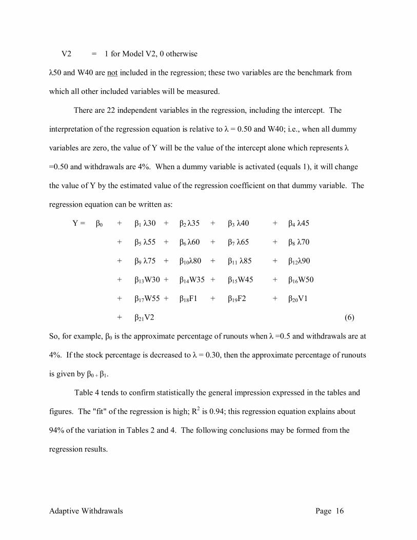
There are 22 independent variables in the regression, including the intercept. The

interpretation of the regression equation is relative to λ = 0.50 and W40; i.e., when all dummy

variables are zero, the value of Y will be the value of the intercept alone which represents λ

=0.50 and withdrawals are 4%. When a dummy variable is activated (equals 1), it will change

the value of Y by the estimated value of the regression coefficient on that dummy variable. The

regression equation can be written as:

Y = β0 + β1 λ30 + β2 λ35 + β3 λ40 + β4 λ45 + β5 λ55 + β6 λ60 + β7 λ65 + β8 λ70 + β9 λ75 + β10λ80 + β11 λ85 + β12λ90 + β13W30 + β14W35 + β15W45 + β16W50 + β17W55 + β18F1 + β19F2 + β20V1 + β21V2 (6)

So, for example, β0 is the approximate percentage of runouts when λ =0.5 and withdrawals are at

4%. If the stock percentage is decreased to λ = 0.30, then the approximate percentage of runouts

is given by β0 + β1.

Table 4 tends to confirm statistically the general impression expressed in the tables and

figures. The "fit" of the regression is high; R2 is 0.94; this regression equation explains about

94% of the variation in Tables 2 and 4. The following conclusions may be formed from the

regression results.


1. The coefficients on λ30 and λ35 are both positive and statistically significant (p < 0.05),

suggesting that λs of 0.30 or 0.35 will result in statistically "less safe" withdrawal strategies

than 4% withdrawal rates at 50/50 stock/bond allocations. λs ≤ 0.35 increases the percentage

of runouts. This increase is not attributable to chance.

2. The coefficients on W30 and W35 are negative and significant (p < 0.001), indicating that,

ceteris paribus, withdrawal rates of less than 4% are "safer" than the 4% withdrawal rate.

Likewise, the coefficients on W45, W50, and W55 are all positive and significant (p <

0.001), indicating that withdrawal rates in excess of 4% result in higher runout percentages

and that these higher percentages are not due to chance. All the results on W30 through W55

confirm what appeared to be clear from the tables, namely that the higher the withdrawal rate

the more like the money was going to run out. These results merely give statistical strength

to those observations.

3. The regression coefficients on all λs except λ30 and λ35 are not significant. This implies that

asset allocation of 0.40 or 0.45 as well as all λs greater than 0.50 are not statistically different

from λ=0.50. While λ =0.50 appears from the table to provide more safety, that contention

cannot be supported statistically.

4. If the withdrawals are not taken at a constant rate, will the portfolio last a longer time or a

shorter time? The regression results for models F1, F2, V1, and V2 confirm much of what

was previously observed. Models F1 and F2 are not statistically different from the

benchmark W40 model. The close general agreement with F1 and the 4% Fixed model in

Figure 1 is consistent with these statistical results. Model V1 is statistically significant in a

two-tailed test only at the 0.10 level. It is however significant in a one-tailed test at the 0.05

level. Model V2 is significant at the 0.01 level. It seems safe to conclude that Models V1


and V2 are "safer" performers than the benchmark. To the extent that V1 provides much

higher average withdrawal percentages, it should be the preferred model for retirees.

V. Conclusions

This study uses a bootstrap simulation to further investigate the probability of running out

of money when making withdrawals from a retirement portfolio. First, results indicate that

Bengen's recommendation that 4% is a "safe" withdrawal rate and 3% is "absolutely safe" may

be optimistic. The risk of a shortfall increases with the amount of the withdrawal and even

withdrawal rates of 3% showed some probability of failing to last 30 years.

Second, the effect of adaptive withdrawal strategies was investigated. Both models V1

and V2 provided higher average withdrawal rates and less likelihood of running out of money

before 30 years had elapsed. Model V1, which withdraws a minimum 4% of the starting

portfolio amount when the portfolio grows, and takes only 3.6% when the portfolio shrinks,

provides the largest withdrawal amounts of the two models.

It should be understood that the outcomes if Model V1 and V2 represent averages and are

not a guarantee. If a person is lucky enough to retire when the market is rising, the rule

expressed by, say, Model V1, allows increasing withdrawal amounts. If the portfolio grows

significantly, even in the face of annual withdrawals, the amount of those withdrawals can safely

increase. If a person is unlucky enough to experience several years of declining portfolio value

at the beginning of retirement, the Model V1 rule requires cutting back on withdrawals. While

the V1 rule allows the retiree to enjoy increasing prosperity, it also requires foregoing some

withdrawals during bad periods. One retiree may start out when the markets are falling for

several years and will probably not attain the average withdrawal amount in Table 3 when

implementing Model V1. Alternately, a retiree may find an economy that is growing and healthy


and may appreciate a much higher withdrawal amount when using Model V1 than is shown in

Table 3. Model V1, however, should provide more safety than the benchmark.

It should be reiterated that the adaptive models presented in this study, like V1 and V2,

are meant as a first step in improving the retiree's experiences. There are many alternative

adaptive models than can be studied, including additional asset classes, such as small-caps, mid-

caps, international stocks, etc. There are ample opportunities for further investigation.


Bibliography Bengen, William P., "Determining Withdrawal Rates Using Historical Data," Journal of Financial Planning, January 1994, pp. 14-24. _______________, "Asset Allocation for a Lifetime," Journal of Financial Planning, August 1996, pp. 58-67. _______________, "Conserving Client Portfolios During Retirement, Part III," Journal of Financial Planning, December 1997, 10, 4, pp. 84-97. ________________, “Conserving Client Portfolios During Retirement, Part IV,” Journal of Financial Planning, May 2001, 14, 5, pp. 110-119. _______________, "Determining Withdrawal Rates Using Historical Data," Journal of Financial Planning, March 2004, pp. 64-73. Bodie, Zvi, Merton Robert C. and Samuelson William F. (1992), “Labor Supply Flexibility and Portfolio Choice in a Life Cycle Model,” Journal of Economic Dynamics and Control, 16, 3-4, 427-449. Cooley, P. L., Hubbard, C. M. & Walz, D. T. (1998), “Retirement Savings: Choosinga Withdrawal Rate that is Sustainable,” AAII Journal, February, 16-21. ______________ “ Sustainable Withdrawal Rates From Your Retirement Portfolio,” Financial Counseling and Planning, 1999, 10(1), 39-47. ______________ “ Retirement Withdrawals: What Rate is Safe When Time is Short and Uncertain,” AAII Journal, January, 4-9. ______________, “A Comparative Analysis of Retirement Portfolio Success Rates: Simulation Versus Overlapping Periods,” Financial Services Review, Summer 2003, Vol. 12 Issue 2, p115-29. Dammon, Robert M., Spatt, Chester S., Zhang, & Harold, H. (2004), “Optimal Asset Location and Allocation with Taxable and Tax-Deferred Investing ,” Journal of Finance, , 59 (3), 999-1038. Dus, Ivica, Maurer, Raimond & Mitchell, Olivia S. (2005), “Betting on Death and Capital Markets in Retirement: A Shortfall Risk Analysis of Life Annuities versus Phased Withdrawal Plans,” Financial Services Review, 14 (3), 169-196. Dybvig, Philip H. (1999), “Using Asset Allocation to Protect Spending,” Financial Analysts Journal, 55 (1), 49–62.


Guyton, William T., “Decision Rules for Portfolio Management for Retirees: Is the ‘Safe’ Initial Withdrawal Rate Too Safe?” Journal of Financial Planning, Oct2004, Vol. 17 Issue 10, 54 - 61 Horan, Stephen M., “Choosing Between Tax-advantaged Savings Accounts: A Reconciliation of Standardized Pretax and After-tax Frameworks,” Financial Services Review, Winter2003, Vol. 12, Issue 4, p339-58. Ibbotson Associates, Stocks, Bonds, Bills and Inflation, EnCorr Database 2004 Edition, Roger Ibbotson and Associates, Chicago, IL. Jagannathan, Ravi and Kocherlakota, Narayana R. (1996), “Why Should Older People Invest Less in Stocks than Younger People?” Quarterly Review of the Federal Reserve Bank of Minneapolis, 20, 3, 11-24. Jones, Charles P. and Wilson, Jack W., (1999), "Asset Allocation Decisions - Making the Choice Between Stocks and Bonds," Journal of Investing, 8(1), 51-56. Kwok, Ho, Milevsky, Moshe Arye & Robinson, Chris, “Asset Allocation, Life Expectancy and Shortfall,” Financial Services Review, 1994, Vol. 3 Issue 2, p109-27. Malkiel, Burton G. (1999). A Random Walk Down Wall Street, 6th Edition, W. W. Norton & Company, New York, NY, 368-371. Milevsky, Moshe M., Kwok, Ho and Robinson, Chris (1997), “Asset Allocation Via The Conditional First Exit Time or How To Avoid Outliving Your Money,” Review of Quantitative Finance and Accounting, 9 (1), 53-70. Modigliani France and Brumberg R. (1954), “Utility Analysis and the Consumption Function,” in K. K. Kurihara, ed., Post Keynesian Economics, New Brunswick, NJ. Opiela, Nancy (2004), “Retirement Distributions: Creating a Limitless Income Stream for an ‘Unknowable Longevity’,” Journal of Financial Planning, 17, 2, 36-42. Ragsdale, Cliff T., Seila, Andrew F. and Little, Philip L., “An Optimization Model for Scheduling Withdrawals from Tax-Deferred Retirement Accounts,” Financial Services Review, 1994, 3, 2, p93-109. Reilly, Frank K. and Brown, Keith C. (2003), Investment Analysis and Portfolio Management, 7th Edition, Thomson- Southwestern, Mason, OH. Tezel, Ahmet (2005), “Sustainable Retirement Withdrawals,” Journal of Financial Planning, 18, 3, 52-57. Vora, Premal P., and McGinnis, John D. (2000), “The Asset Allocation Decision in Retirement: Lessons from Dollar Cost Averaging,” Financial Services Review, 9 (1), 47-63.

Table 1

A. Summary of Research Literature on Endowment Withdrawal Rates

Author(s) Dates Journal (s) Methodology Results Bengen 1994, 1996, 1997,

2001 & 2004 All appear in Journal of Financial Planning

Overlapping period methodology Optimal withdrawal rate of 4.1% to 4.3%.

Cooley, Hubbard and Walz

2003 1998, 1999, 2005

Financial Services Review Journal of Financial Counseling and Planning, AAII Journal

Overlapping periods and simulations 4% withdrawal rate with at least 50% in stocks and success rate of 75% as acceptable.

Dus, Maurer & Mitchell

2005

Financial Services Review

Phased withdrawal

Fixed withdrawal rate as a rate of current (not initial) portfolio and later annutization lowest shortfall risk.

Dybvig 1999 Financial Analysts Journal Back testing, historical return replication Higher withdrawals during consistently up and down markets.

Guyton 2004 Journal of Financial Planning Constant asset class weights. Conditional withdrawals. Methodology not described adequately for replication.

Optimal withdrawal rate of 4.2% to 5.7%.

Pye 2000 1999, 2000, 2001

Journal of Portfolio Management Journal of Financial Planning

Probabilistic model with TIPs as part of the asset allocation

High allocation to TIPs increases safe payout from 4 to 4.5 percent.

Ragsdale, Seila and Little

1994 Financial Services Review Mathematical programming model for withdrawals from tax deferred accounts

Conditional withdrawal model dependent on various variables.

Tezel 2004 Journal of Financial Planning Monte Carlo Optimal withdrawal rate of 2.68% to 4.83%. Vora and McGinnis

2000 Financial Services Review Dollar cost disinvesting Greatest withdrawals with a 100 percent stock portfolio.

Table 2. Percentage of Times that Portfolio Runs out of Money, by λ and Withdrawal Amount (Shaded cells are Row Minimums)

Withdrawal λ

Amount 0.30 0.35 0.40 0.45 0.50 0.55 0.60 0.65 0.70 0.75 0.80 0.85 0.90 3.0 1.13 1.20 1.07 1.35 1.28 1.39 1.92 1.76 2.12 2.38 3.16 3.29 3.94

3.5 4.33 3.67 3.68 3.59 3.67 3.81 3.85 4.06 4.74 4.92 5.50 5.79 6.74

4.0 9.69 8.70 8.11 7.38 6.72 7.77 7.79 7.62 8.51 8.74 9.13 9.11 10.16

4.5 16.75 15.78 14.76 13.42 12.86 12.74 12.30 12.07 12.87 13.26 13.16 13.66 14.47

5.0 28.49 25.56 23.57 20.33 20.61 20.02 18.71 17.86 18.53 17.92 19.01 18.29 20.13

5.5 41.26 36.86 32.83 31.19 29.18 27.03 26.31 24.72 24.63 24.87 24.00 24.47 24.71

Table 3. Average Withdrawal Amount as a percent of Initial Portfolio, by λ and by Model

λ

Model 0.30 0.35 0.40 0.45 0.50 0.55 0.60 0.65 0.70 0.75 0.80 0.85 0.90 F1 4.13 4.12 4.13 4.15 4.15 4.15 4.14 4.14 4.13 4.14 4.14 4.13 4.14

F2 3.87 3.88 3.87 3.85 3.85 3.84 3.86 3.86 3.87 3.86 3.86 3.87 3.86

V1 4.66 4.84 5.00 5.21 5.48 5.73 5.91 6.24 6.47 6.77 7.21 7.50 7.97

V2 4.10 4.20 4.26 4.29 4.40 4.49 4.64 4.77 4.95 5.06 5.21 5.44 5.51

Table 4. Percentage of Times that Portfolio Runs out of Money,

by λ and by Model 4% Fixed and Adaptive Models F1,F2,V1,V2

(Shaded cells are Row Minimums)

λ Model 0.30 0.35 0.40 0.45 0.50 0.55 0.60 0.65 0.70 0.75 0.80 0.85 0.90

4% Fixed 9.69 8.70 8.11 7.38 6.72 7.77 7.79 7.62 8.51 8.74 9.13 9.11 10.16

F1 10.11 8.27 7.87 7.73 7.54 8.05 7.57 8.16 8.47 8.63 9.37 9.88 10.48

F2 8.67 8.04 6.94 6.45 7.04 6.77 7.31 7.39 7.50 8.50 8.51 9.53 9.37

V1 7.41 6.41 6.04 5.95 6.26 5.76 6.34 6.81 6.13 7.33 7.85 8.71 8.66

V2 7.08 6.34 5.75 5.69 5.34 5.37 6.04 6.23 6.38 6.64 7.31 7.67 8.20

FIG URE 1. Pe rce nt R unouts (Sm alle r is B e tte r) for v arious λ and M ode ls

5%

6%

7%

8%

9%

10%

11%

12%

30% 35% 40% 45% 50% 55% 60% 65% 70% 75% 80% 85% 90%

Pe rce nt of Stocks

Perc

ent R

unou

ts

4% FixedF1V1V2

FIGURE 2. Average Withdrawal Percentages (Bigger is Better) for various λ and Models

3.5

4

4.5

5

5.5

6

6.5

7

7.5

8

8.5

30% 35% 40% 45% 50% 55% 60% 65% 70% 75% 80% 85% 90%

Percent of Stocks

Perc

ent W

ithdr

awal

s

4% FixedF1V1V2

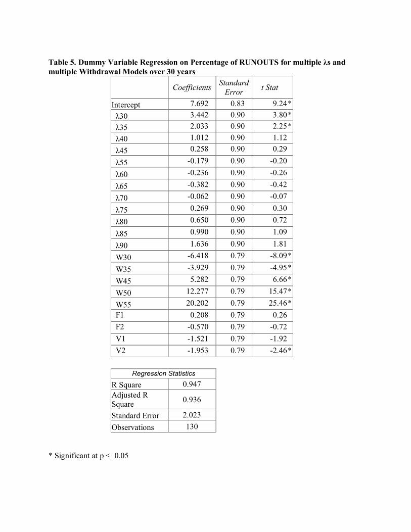
Table 5. Dummy Variable Regression on Percentage of RUNOUTS for multiple λs and multiple Withdrawal Models over 30 years

Coefficients Standard

Error t Stat

Intercept 7.692 0.83 9.24 * λ30 3.442 0.90 3.80 * λ35 2.033 0.90 2.25 * λ40 1.012 0.90 1.12 λ45 0.258 0.90 0.29

λ55 -0.179 0.90 -0.20

λ60 -0.236 0.90 -0.26

λ65 -0.382 0.90 -0.42

λ70 -0.062 0.90 -0.07

λ75 0.269 0.90 0.30

λ80 0.650 0.90 0.72

λ85 0.990 0.90 1.09

λ90 1.636 0.90 1.81

W30 -6.418 0.79 -8.09 *

W35 -3.929 0.79 -4.95 *

W45 5.282 0.79 6.66 *

W50 12.277 0.79 15.47 *

W55 20.202 0.79 25.46 * F1 0.208 0.79 0.26 F2 -0.570 0.79 -0.72 V1 -1.521 0.79 -1.92 V2 -1.953 0.79 -2.46 *

Regression Statistics

R Square 0.947

Adjusted R Square 0.936

Standard Error 2.023

Observations 130

* Significant at p < 0.05

1 The bootstrap allows repeated sampling from a relatively small population but from which statistically valid conclusions may be drawn. One of the 78 years is randomly selected each time; rates of return that actually occurred are selected and the differences (spreads) between stock returns and bond returns in that year are historically correct. The number of possible sequences (orderings) of the rates of return is extremely large and the sequence will influence the success or failure of the withdrawal process. Since sampling is with replacement, there are 78 ways to select the first year, and 78 ways to select the second year, etc. All told there are 7830 ≈ 5.8*1056 different 30-year sequences. The bootstrap looks at a mere 10,000 sequences for each of the possible conditions.

adaptive withdrawals - retail investor .org · adaptive withdrawals abstract for individual...

Documents