Adaptively Processing Remote Dataand Learning Source Mappings

Zachary G. IvesUniversity of Pennsylvania

CIS 650 – Database & Information Systems

March 14, 2005

LSD Slides courtesy AnHai Doan

2

Administrivia

Midterm due 3/16 5-10 pages (single-spaced, 10-12 pt) If you haven’t told me which topic, please

do so now!

3

Today’s Trivia Question

4

Many Motivations for Adaptive Query Processing

Many domains where cost-based query optimization fails:

Complex queries in traditional databases: estimation error grows exponentially with # joins [IC91]; the focus of [KD98], [M+04]

Querying over the Internet: unpredictable access rates, delays

Querying external data sources: limited information available about properties of this source

Monitor real-world conditions, adapt processing strategy in response

5

Generalizing Adaptive Query Processing

We’ve seen a range of different adaptive techniques

How do they fit together? Can we choose points between eddies and

mid-query re-optimization? Can we exploit other kinds of query optimization “tricks”?

6

Popular Types of Adaptive Query Processing

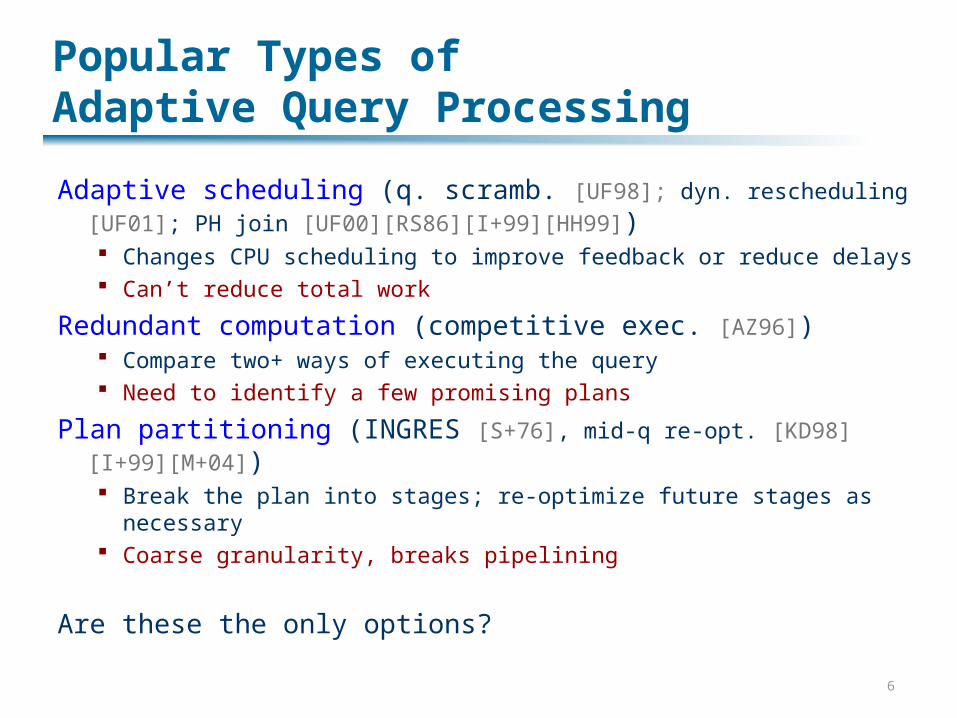
Adaptive scheduling (q. scramb. [UF98]; dyn. rescheduling [UF01]; PH join [UF00][RS86][I+99][HH99]) Changes CPU scheduling to improve feedback or reduce delays Can’t reduce total work

Redundant computation (competitive exec. [AZ96]) Compare two+ ways of executing the query Need to identify a few promising plans

Plan partitioning (INGRES [S+76], mid-q re-opt. [KD98][I+99][M+04]) Break the plan into stages; re-optimize future stages as

necessary Coarse granularity, breaks pipelining

Are these the only options?

7

Two More Forms of Adaptivity

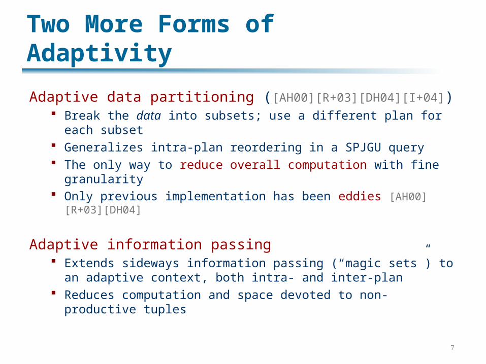
Adaptive data partitioning ([AH00][R+03][DH04][I+04]) Break the data into subsets; use a different plan for each

subset Generalizes intra-plan reordering in a SPJGU query The only way to reduce overall computation with fine

granularity Only previous implementation has been eddies [AH00][R+03]

[DH04]

Adaptive information passing Extends sideways information passing (“magic sets”) to an

adaptive context, both intra- and inter-plan Reduces computation and space devoted to non-productive

tuples

8

Eddies Combine Adaptive Scheduling and Data Partitioning Decisions

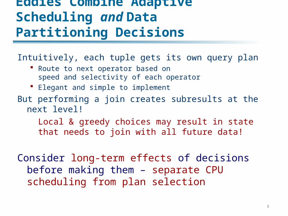
Intuitively, each tuple gets its own query plan Route to next operator based on

speed and selectivity of each operator Elegant and simple to implement

But performing a join creates subresults at the next level!

Local & greedy choices may result in state that needs to join with all future data!

Consider long-term effects of decisions before making them – separate CPU scheduling from plan selection

9

Focusing Purely on Adaptive Data Partitioning

Use adaptively scheduled operators to “fill CPU cycles”

Now a query optimizer problem:Choose a plan that minimizes long- term cost (in CPU cycles)

To allow multiple plans, distribute union through join (and select, project, etc.):

If R1 = R11 [ R1

2, R2 = R21 [ R2

2 then:

R1 ⋈ R2 = (R11 [ R1

2) ⋈ (R21 [ R2

2) =

(R11 ⋈ R2

1) [ (R12 ⋈ R2

2) [ (R1

1 ⋈ R22) [ (R1

2 ⋈ R21)

R1R2

R11 R2

1

R12 R2

2

This generalizes to njoins, other SPJ + GU

operators…

10

Adaptive Data Partitioning:Routing Data across Different Plans

R ⋈ S ⋈ T

Exclude R0S0

Exclude R0S0T0,R1S1T1

R0S 0

R1

T1

S 1

T0

R0 S 0

R S T

R0 S0T0

R0 S0 …

S0R0

T 0 S1T1

R1 S1T1

R1

S 1 T1

Options for combining across phases: New results

always injected into old plan

Old results into new plan

Wait until the end – “stitch-up” plan based on best stats

11

Special Architectural Features for ADP

Monitoring and re-optimization thread runs alongside execution:

System-R-like optimizer with aggregation support;uses most current selectivity estimates

Periodic monitoring and re-optimization revises selectivity estimates, recomputes expected costs

Query execution with “smart router” operatorsSpecial support for efficient stitch-up plans:

Uses intermediate results from previous plans (specialized-case of answering queries using views [H01])

Join-over-union (“stitch-up-join”) operator that excludes certain results

12

ADP Application 1:Correcting Cost Mis-estimates

Goal: react to plans that are obviously bad Don’t spend cycles searching for a slightly better plan Try to avoid paths that are likely to not be promising

Monitor/reoptimizer thread watches cardinalities of subresults Re-estimate plan cost, compare to projected costs of

alternatives, using several techniques & heuristics (see paper) Our experiments: re-estimate every 1 sec.

“Smart router” operator does the following: Waits for monitor/reoptimizer to suggest replacement plan Re-routes source data into the new plan New plan’s output is unioned with output of previous plan;

this is fed into any final aggregation operations

13

Correcting for Unexpected Selectivities

04

08

0

3A(uniform)

3A(skewed)

10(uniform)

10(skewed)

10A(uniform)

10A(skewed)

5(uniform)

5(skewed)

Query - data set combination

Ru

nn

ing

tim

e (s

ec)

Static - No StatisticsStatic - CardinalitiesAdaptive - No StatisticsAdaptive - CardinalitiesPlan Partitioning - No Stats

119 122 164 171 163 172 148 149 Pentium IV 3.06 GHzWindows XP

14

ADP Application 2:Optimizing for Order

Most general ADP approach: Pre-generate plans for general

case and each “interesting order” “Smart router” sends tuple to the

plan whose ordering constraint is followed by this tuple

But with multiple joins, MANY plans

Instead: do ADP at the operator level “Complementary join pair” Does its own stitch-up internally Easier to optimize for!

Can also do “partial sorting” at the router (priority queue)

Q Q

Q

QQ

MergeHash

R S

h(R) h(S) h(R) h(S)

...

Routers

15

Exploiting Partial Order in the Data

0

82

164

Uniform Skewed Uniform,1%

Reordered

Skewed,1%

Reordered

Skewed,10%

Reordered

Skewed,50%

Reordered

Data set

Ru

nn

ing

Tim

e (

se

c)

Pipelined hash join

Complementary joins

Comp. joins with priority queue

(1024 tuple)

Pentium IV 3.06 GHzWindows XP

16

ADP Over “Windows”:Optimizing for Aggregation

Group-by optimization [CS94]: May be able to “pre-aggregate” some

tuples before joining Why: aggregates can be applied over

union But once we insert pre-

aggregation, we’re stuck (and it’s not pipelined)

Our solution: “Adjustable window pre-aggregation” Change window size depending on

how effectively we can aggregate Also allows data to propagate through

the plan – better info for adaptivity, early answers

T

R

SUM(T.y sums)GROUP BY T.x

SUM(T.y)GROUP BY

T.x, T.joinAttrib

T R

SUM(T.y)GROUP BY T.x

vs.

17

Pre-Aggregation Comparison

0

20

40

3A(uniform)

10(uniform)

10A(uniform)

5(uniform)

Query - data set combination

Ru

nn

ing

Tim

e (

se

c)

Single Aggregation

Traditional Pre-Aggregation

Adjustable-Window Pre-Aggregation

147 149 149 141

18

The State of the Union Join and Agg

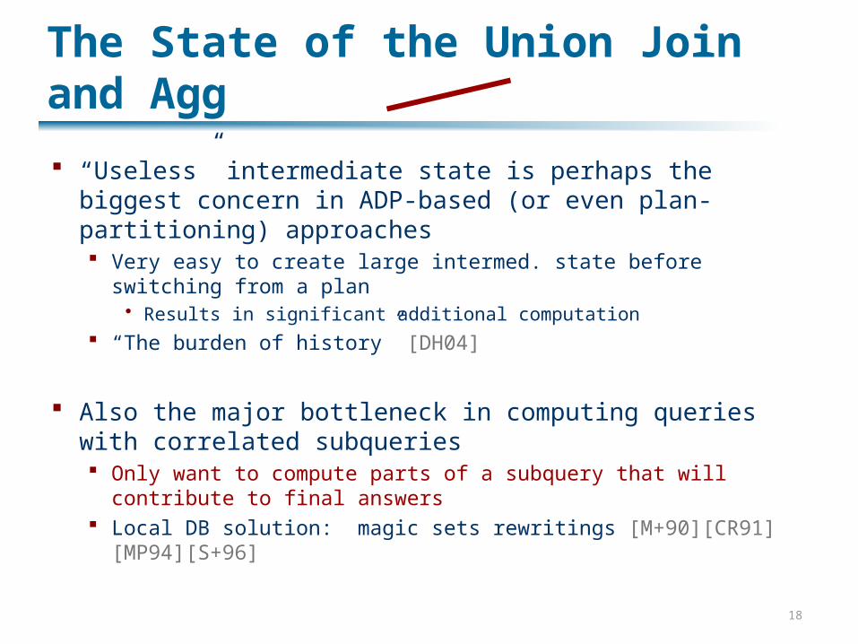
“Useless” intermediate state is perhaps the biggest concern in ADP-based (or even plan-partitioning) approaches Very easy to create large intermed. state before switching from

a plan Results in significant additional computation

“The burden of history” [DH04]

Also the major bottleneck in computing queries with correlated subqueries Only want to compute parts of a subquery that will contribute to

final answers Local DB solution: magic sets rewritings [M+90][CR91][MP94]

[S+96]

19

Intuition behind Magic Sets Rewritings

Observations: Computing a subquery once for every iteration of the

outer query is repetitive, inefficient Computing the subquery in its entirety is also frequently

inefficient

So “pass in” information about specifically which tuples from the inner query might join with the outer query A “filter set” – generally a projection of a portion of the

outer query results Anything that joins with the parent block must join with

the filter set False positives are OK

20

Query with Magic SetCREATE VIEW TotalSales(SellerID, Sales, ItemsSold) SELECT SellerID, sum(salePrice) AS Sales, count(*) AS ItemsSold FROM SellerList SL, SaleItem S WHERE SL.SellerID = S.SellerID GROUP BY SL.SellerID

SELECT SellerID, Sales, ItemsSold FROM TotalSales TS, Recommended REC, Ratings RAT WHERE REC.SellerID = TS.SellerID AND RAT.SellerID = TS.SellerID AND RAT.Rating > 4 AND ItemsSold > 50

21

Query with Magic Set [S+96]

*

*

CREATE VIEW TotalSales(SellerID, Sales, ItemsSold) SELECT SellerID, sum(salePrice) AS Sales, count(*) AS ItemsSold FROM SellerList SL, SaleItem S WHERE SL.SellerID = S.SellerID GROUP BY SL.SellerID

SELECT SellerID, Sales, ItemsSold FROM TotalSales TS, Recommended REC, Ratings RAT WHERE REC.SellerID = TS.SellerID AND RAT.SellerID = TS.SellerID AND RAT.Rating > 4 AND ItemsSold > 50

22

Magic in Data Integration

In data integration: Difficult to determine when to do sideways information

passing/magic in a cost-based way Magic optimization destroys some potential parallelism

– must compute outer block first Opportunities:

Pipelined hash joins give us complete state for every intermediate result

We use bushy trees

Our idea: do information passing out-of-band Consider a plan as if it’s a relational calculus expression

– every tuple must satisfy constraints The plan dataflow enforces this… … But we can also pass information

across the plan outside the normal dataflow

A B

Cx

x

23

Adaptive Information Passing

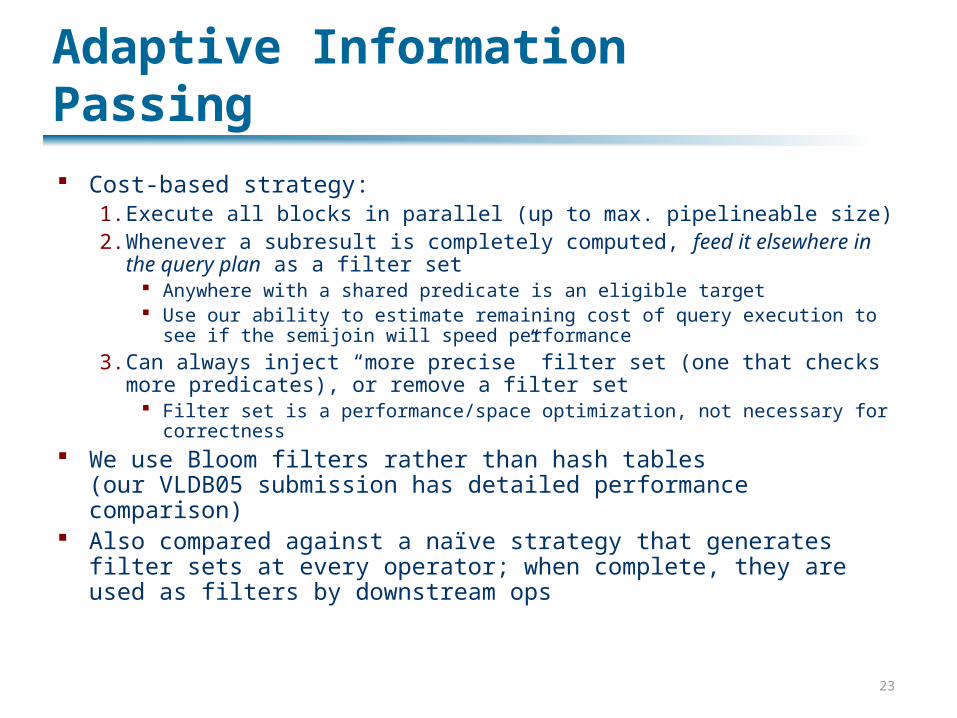
Cost-based strategy:1. Execute all blocks in parallel (up to max. pipelineable size)2. Whenever a subresult is completely computed, feed it elsewhere

in the query plan as a filter set Anywhere with a shared predicate is an eligible target Use our ability to estimate remaining cost of query execution to see if

the semijoin will speed performance

3. Can always inject “more precise” filter set (one that checks more predicates), or remove a filter set

Filter set is a performance/space optimization, not necessary for correctness

We use Bloom filters rather than hash tables(our VLDB05 submission has detailed performance comparison)

Also compared against a naïve strategy that generates filter sets at every operator; when complete, they are used as filters by downstream ops

24

Tuples Created – TPC-H, 1GB(~67% savings in Q2. Also savings in Q5, not shown)

0.0E+00

5.0E+06

1.0E+07

1.5E+07

TPC-2-1G TPC-17-1G IBM-1G

Query

Tu

ple

s s

tore

d

AIP Normal Magic sets Feed-forward

25

Adaptive QP in Summary

A variety of different techniques, focusing on: Scheduling Comparison & competition Data + plan partitioning Information passing

A field that is still fairly open – missing: Effective exploration methods A true theory!

What’s possible? What kinds of queries make sense to adapt?

Guarantees of optimality and convergence (perhaps under certain assumptions)

26

Switching from Low-Level to High-Level

We’ve talked about: Query reformulation (composing queries with

mappings) Query optimization + execution

But how did we ever get the mappings in the first place? This is one of the most tedious tasks

Answer: LSD (and not the kind that makes you high!) … Slides courtesy of AnHai Doan, UIUC

27

Semantic Mappings between Schemas Mediated & source schemas = XML DTDs

house

location contact

house

address

name phone

num-baths

full-baths half-baths

contact-info

agent-name agent-phone

1-1 mapping non 1-1 mapping

28

Suppose user wants to integrate 100 data sources

1. User manually creates mappings for a few sources, say 3 shows LSD these mappings

2. LSD learns from the mappings “Multi-strategy” learning incorporates many types of

info in a general way Knowledge of constraints further helps

3. LSD proposes mappings for remaining 97 sources

The LSD (Learning Source Descriptions) Approach

29

listed-price $250,000 $110,000 ...

address price agent-phone description

Example

location Miami, FL Boston, MA ...

phone(305) 729 0831(617) 253 1429 ...

commentsFantastic houseGreat location ...

realestate.com

location listed-price phone comments

Schema of realestate.com

If “fantastic” & “great”

occur frequently in data values =>

description

Learned hypotheses

price $550,000 $320,000 ...

contact-phone(278) 345 7215(617) 335 2315 ...

extra-infoBeautiful yardGreat beach ...

homes.com

If “phone” occurs in the name =>

agent-phone

Mediated schema

30

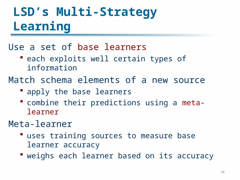
LSD’s Multi-Strategy Learning

Use a set of base learners each exploits well certain types of information

Match schema elements of a new source apply the base learners combine their predictions using a meta-learner

Meta-learner uses training sources to measure base learner

accuracy weighs each learner based on its accuracy

31

Base Learners Input

schema information: name, proximity, structure, ...

data information: value, format, ... Output

prediction weighted by confidence score Examples

Name learner agent-name => (name,0.7), (phone,0.3)

Naive Bayes learner “Kent, WA” => (address,0.8), (name,0.2) “Great location” => (description,0.9), (address,0.1)

32

<location> Boston, MA </> <listed-price> $110,000</> <phone> (617) 253 1429</> <comments> Great location </>

<location> Miami, FL </> <listed-price> $250,000</> <phone> (305) 729 0831</> <comments> Fantastic house </>

Training the Learners

Naive Bayes Learner

(location, address)(listed-price, price)(phone, agent-phone)(comments, description) ...

(“Miami, FL”, address)(“$ 250,000”, price)(“(305) 729 0831”, agent-phone)(“Fantastic house”, description) ...

realestate.com

Name Learner

address price agent-phone description

Schema of realestate.com

Mediated schema

location listed-price phone comments

33

<extra-info>Beautiful yard</><extra-info>Great beach</><extra-info>Close to Seattle</>

<day-phone>(278) 345 7215</><day-phone>(617) 335 2315</><day-phone>(512) 427 1115</>

<area>Seattle, WA</><area>Kent, WA</><area>Austin, TX</>

Applying the Learners

Name LearnerNaive Bayes

Meta-Learner

(address,0.8), (description,0.2)(address,0.6), (description,0.4)(address,0.7), (description,0.3)

(address,0.6), (description,0.4)

Meta-LearnerName LearnerNaive Bayes

(address,0.7), (description,0.3)

(agent-phone,0.9), (description,0.1)

address price agent-phone description

Schema of homes.com Mediated schema

area day-phone extra-info

34

Domain Constraints Impose semantic regularities on sources

verified using schema or data

Examples a = address & b = address a = b a = house-id a is a key a = agent-info & b = agent-name b is nested

in a

Can be specified up front when creating mediated schema independent of any actual source schema

35

area: address contact-phone: agent-phoneextra-info: description

area: address contact-phone: agent-phoneextra-info: address

area: (address,0.7), (description,0.3)contact-phone: (agent-phone,0.9), (description,0.1)extra-info: (address,0.6), (description,0.4)

The Constraint Handler

Can specify arbitrary constraints User feedback = domain constraint

ad-id = house-id Extended to handle domain heuristics

a = agent-phone & b = agent-name a & b are usually close to each other

0.30.10.40.012

0.70.90.60.378

0.70.90.40.252

Domain Constraintsa = address & b = adderss a = b

Predictions from Meta-Learner

36

Putting It All Together: LSD System

L1 L2 Lk

Mediated schema

Source schemas

Data listings

Training datafor base learners Constraint Handler

Mapping Combination

User Feedback

Domain Constraints

Base learners: Name Learner, XML learner, Naive Bayes, Whirl learner Meta-learner

uses stacking [Ting&Witten99, Wolpert92] returns linear weighted combination of base learners’ predictions

Matching PhaseTraining Phase

37

Empirical Evaluation

Four domains Real Estate I & II, Course Offerings, Faculty

Listings

For each domain create mediated DTD & domain constraints choose five sources extract & convert data listings into XML mediated DTDs: 14 - 66 elements, source DTDs:

13 – 48 Ten runs for each experiment - in each run:

manually provide 1-1 mappings for 3 sources ask LSD to propose mappings for remaining 2 sources accuracy = % of 1-1 mappings correctly identified

38

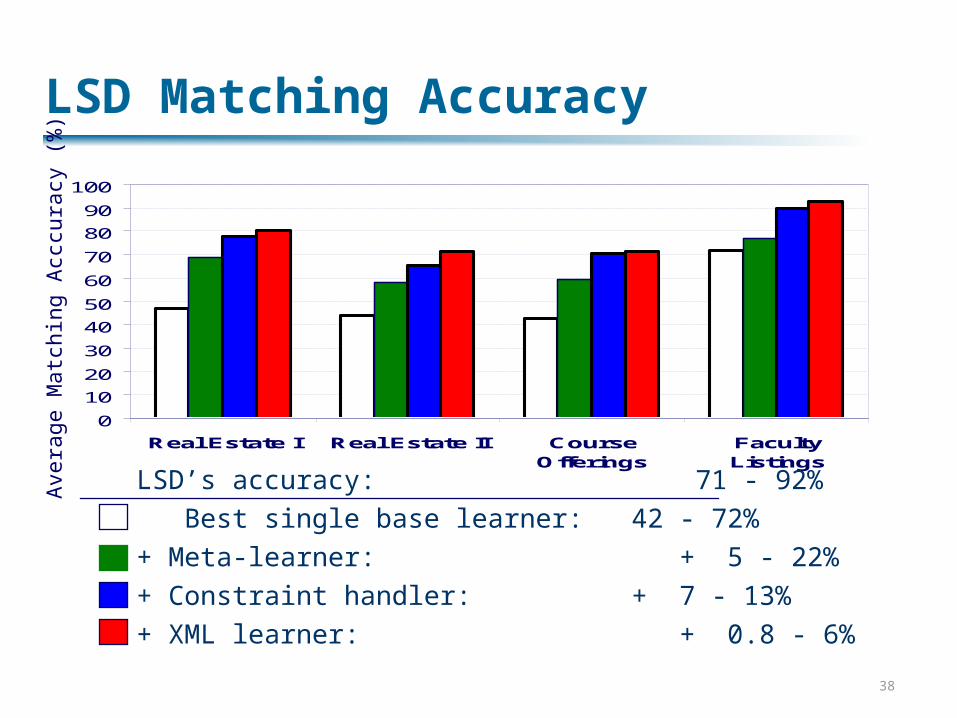
LSD Matching Accuracy

0

10

20

30

40

50

60

70

80

90

100

Real Estate I Real Estate II CourseOfferings

FacultyListings

LSD’s accuracy: 71 - 92% Best single base learner: 42 - 72%+ Meta-learner: + 5 - 22%+ Constraint handler: + 7 - 13%+ XML learner: + 0.8 - 6%

Ave

rage

Mat

chin

g A

cccu

racy

(%

)

39

LSD Summary

Applies machine learning to schema matching use of multi-strategy learning Domain & user-specified constraints

Probably the most flexible means of doing schema matching today in a semi-automated way

Complementary project: CLIO (IBM Almaden) uses key and foreign-key constraints to help the user build mappings

40

Jumping Up a Level

We’ve now seen how distributed data makes a huge difference … In heterogeneity and the need for relating

different kinds of attributes Mapping languages Mapping tools Query reformulation

… and in query processing Adaptive query processing