addis ababauniversity institute of biotechnology
TRANSCRIPT

ADDIS ABABAUNIVERSITY
INSTITUTE OF BIOTECHNOLOGY
Ethnobotanical Knowledge of Lablab (Lablab purpureus (L.) Sweet -
Fabaceae) in Konso zone and genetic diversity of collections from Ethiopia
using SSR markers
MSc. Thesis
Solomon Tamiru Workneh
October, 2020
Addis Ababa, Ethiopia

ii
ADDIS ABABAUNIVERSITY
INSTITUTE OF BIOTECHNOLOGY
Ethnobotanical Knowledge of Lablab (Lablab purpureus (L.) Sweet- Fabaceae)
in Konso zone and genetic diversity of collections from Ethiopia using SSR
markers
MSc. Thesis
Submitted to the Institute of Biotechnology for the partial fulfillment of the
requirements for the degree of Master of Science in Biotechnology
By
Solomon Tamiru Workneh
October, 2020
Addis Ababa, Ethiopia

iii
ADDIS ABABA UNIVERSITY
INSTITUTE OF BIOTECHNOLOGY
MSc. THESIS APPROVAL SHEET
This is to certify that the thesis prepared by Solomon Tamiru, entitled “Ethnobotanical
Knowledge of Lablab (Lablab purpureus (L.) Sweet - Fabaceae) in Konso zone and genetic
diversity of collections from Ethiopia using SSR markers” submitted in partial fulfillment of
the requirements for the Degree of Master of Science in Biotechnology complies with the
regulations of the University and meets the standard with respect to originality and quality.
Signed by the Examining Committee:
Demesachew Guadie (PhD) IoB, AAU ________________ _______________
Internal Examiner Signature Date
Ermias Lulekal (PhD) PBBM, AAU _________________ ________________
External Examiner Signature Date
Tileye Feyisa (PhD) IoB, AAU _________________ _________________
Main advisor Signature Date
Zemede Asfaw (Prof.) PBBM, AAU ________________ __________________
Co- advisor Signature Date
Tesfaye Disasa (PhD) NABRC, EIAR ________________ ___________________
Co- advisor Signature Date
Tesfaye Sisay (PhD) _________________ _________________
Director, Institute of Biotechnology Signature Date

i
ABSTRACT
Ethnobotanical Knowledge of Lablab (Lablab purpureus (L.) Sweet - Fabaceae) in Konso zone
and genetic diversity of collections from Ethiopia using SSR markers
Solomon Tamiru Workneh, MSc. Thesis
Addis Ababa University, 2020
Lablab is an important multipurpose legume crop used for human consumption, animal feed and
soil conservation. In spite of these qualities, the potential value of this crop has not been fully
utilized, and little research attention has been given to this crop. The main objective of the study
was to build the knowledge base from farmers’ perspectives and molecular genetic diversity
analysis of Lablab collections using 15 SSR markers. The field study was conducted in December
2018 in six kebeles distributed in Konso zone by interviewing a total of 84 informants containing
72 randomly selected general informants and 12 purposively selected key informants (42 men
and 42 women) of above 18 years age. The data were analyzed by entering the data into the
excel spreadsheet version 2007 and summarized using descriptive statistics. A total of six Lablab
farmers’ varieties were identified and the majority of the farmers give names to their varieties
based on seed color. The main cultivation practices in the study area were intercropping Lablab
with sorghum, maize and finger millet, and sole crop in the margin of terracing and fence line. In
Konso zone, Lablab is mainly used for human food in the form of boiled grain (NIFRO), animal
feed and soil conservation purpose. The molecular genetic diversity study of 91 lablab
collections from the entire country revealed a total of 225 alleles with an average of 14.80
alleles per locus. All markers across the entire populations were found to be highly polymorphic
and informative with PIC values ranging from 0.92 to 0.78 with a mean value of 0.85. The
average expected heterozygosity and gene diversity was 0.75 and 0.86 respectively, indicating a
high level of genetic diversity. Analysis of molecular variance showed that 94% of the total
genetic variation was attributed to within populations while only 6% was attributed to among
populations. The smaller Fixation Index value (0.061) recorded indicates the presence of
moderate population differentiation as a result of higher gene flow (Nm =3.820) among
populations. Cluster, PCoA and Structure analysis revealed a weak association between
geographical origin and genetic diversity confirming the presence of population admixtures due
to seed exchange and sharing. The observed higher genetic diversity in Konso and West Wellega
zones indicates hot spot area for genetic diversity and germplasm evaluation. Generally,
ethnobotanical knowledge and genetic diversity obtained from this study provides inputs for
Lablab conservation and improvement in Ethiopia.
Keywords/Phrases: Ethnobotany, Gene diversity, General informants, Heterozygosity, Key
informants, Polymorphic

ii
ACKNOWLEDGMENTS
On top of everything, I would like express my gratitude to the Almighty God for his endless
opportunity and help that enabled me to complete my study successfully.
First of all I would like to express my particular gratitude and deepest appreciation to my
supervisors, Dr. Tileye Feyisa, Prof. Zemede Asfaw and Dr. Tesfaye Disasa for their continuous
support, guidance, valuable comments, suggestions and encouragements for the completion of
the research.
I extend my thanks to the Ethiopian Institute of Agricultural Research (EIAR), National
Agricultural Biotechnology Research Center (NABRC) and Addis Ababa University for
the sponsorship and supporting the study program financially. I would like to thank the
Ethiopian Biodiversity Institute (EBI) for providing me the study materials. I also would like to
express my thanks to the McKnight Foundation for their financial, material and training support
received through the Legume Diversity Project administered by the Department of Plant Biology
and Biodiversity Management. I also thank Mr. Demeke Mekonen (GIS experts from EIAR) for
his technical support in mapping the study area.
My Special appreciation goes to all staff members of plant biotechnology, particularly Kalkidan
Tesfu, Messele Molla, Lidiya Ashenafi and Yetaseb Nigusu for their technical assistance during
molecular laboratory work. My special appreciation also goes to Konso farmers for their kind
spent of their time and for sharing their knowledge during sample collection. I also express my
gratitude to Sisaye Aregaye for his support during field data collection and his genuine
cooperation in every aspect of the research.

iii
Finally, I would like to express my very profound gratitude to my dear family to Fasika
Alebachew, Tamiru Workneh, my mother Qelemua Kifleand other close relatives for their
continuous support, encouragement and patience throughout the period of my study. Last but not
least, I would like to thank Mesfin Tadele for his strong contributions in the entire period of this
work.

iv
TABLE OF CONTENTS
Contents Page
ABSTRACT ..................................................................................................................................... i
ACKNOWLEDGMENTS .............................................................................................................. ii
TABLE OF CONTENTS ............................................................................................................... iv
LIST OF FIGURES ...................................................................................................................... vii
LIST OF TABLES ....................................................................................................................... viii
LIST OF APPENDICES ................................................................................................................ ix
LIST of ABBREVIATIONS........................................................................................................... x
CHAPTER ONE ............................................................................................................................. 1
1.INTRODUCTION ....................................................................................................................... 1
1.1. Background .......................................................................................................................... 1
1.2. Statement of the Problem ..................................................................................................... 2
1.3. Research Questions, Hypotheses and Objectives ................................................................. 3
1.3.1. Research questions ........................................................................................................ 3
1.3.2.Research hypotheses ....................................................................................................... 3
1.3.3. Research objectives ....................................................................................................... 4
CHAPTER TWO ............................................................................................................................ 5
2. LITERATURE REVIEW ........................................................................................................... 5
2.1. Origin and Distribution ........................................................................................................ 5
2.2. Taxonomy of Lablab ............................................................................................................ 6
2.3. Botanical description of Lablab ........................................................................................... 6
2.4. Uses of Lablab ...................................................................................................................... 7
2.5. Environmental requirements of Lablab ................................................................................ 8
2.6. Production constraints .......................................................................................................... 9
2.8. Farmers varieties (landrace) diversity .................................................................................. 9
2.9. Genetic markers used in crop diversity study .................................................................... 10
2.9.1. Morphological markers................................................................................................ 10
2.9.2. Biochemical Markers ................................................................................................... 11
2.9.3. DNA based markers ..................................................................................................... 12

v
CHAPTER THREE ...................................................................................................................... 16
3.MATERIALS AND METHODS ............................................................................................... 16
3.1. Ethnobotanical Field Survey .............................................................................................. 16
3. 1. 1. Description of the Study Area ................................................................................... 16
3.1.2. Materials used .............................................................................................................. 17
3.1.3. Methods ....................................................................................................................... 18
3.2. Molecular Genetic Diversity Study .................................................................................... 20
3. 2.1. Plant materials ............................................................................................................ 20
3.2.2. DNA Extraction ........................................................................................................... 22
3.2.3. Primer selection and optimization ............................................................................... 23
3.2.4. PCR and gel electrophoresis ........................................................................................ 25
3.3. Data Analysis ..................................................................................................................... 26
3.3.1. Ethnobotanical data analysis ....................................................................................... 26
3.3.2. Molecular genetic diversity data scoring and analysis ................................................ 27
CHAPTER FOUR ......................................................................................................................... 29
4.RESULTS .................................................................................................................................. 29
4.1. Ethnobotanical study .......................................................................................................... 29
4.1.1. Legume crops grown in the study area ........................................................................ 29
4.1.2. Diversity of Lablab farmers’ varieties cultivated in Konso zone ................................ 30
4.1.3. Landraces diversity and richness ................................................................................. 32
4.1.4. Intercropping of Lablab with other crops .................................................................... 33
4.1.5. Lablab seed source ....................................................................................................... 33
4.1.5. Gender and age role in cropping of Lablab in Konso zone ......................................... 34
4.1.6. Planting and harvesting time of the crop ..................................................................... 35
4.1.7. Uses of Lablab in the study area .................................................................................. 37
4.1.8. Production constraints of the crop in Konso zone ....................................................... 38
4.2. Molecular genetic diversity ................................................................................................ 38
4.2.2. Genetic relationship within and among populations ................................................... 43
4.2.3. Analysis of molecular variance ................................................................................... 44
4.2.4. Magnitude of genetic distance between populations ................................................... 45
4.2.5 Genetic interrelationships between Lablab accessions ................................................. 46

vi
4.2.6. Principal coordinate analysis (PCOA) ......................................................................... 48
CHAPTER FIVE .......................................................................................................................... 52
5. DISCUSSION CONCLUSION AND RECOMMENDATIONS ............................................. 52
5.1.1. Diversity of farmers’ varieties of Lablab in Konso zone ................................................ 52
5.1.2. Cropping systems and management practice .................................................................. 52
5.1.3. Use of Lablab in the study area ....................................................................................... 53
5.1.4. Gender and age roles in production and management of Lablab in the study area......... 54
5.1.5. Planting month of Lablab in the study area..................................................................... 54
5.1.6. Production constraint of Lablab ...................................................................................... 55
5.1.7. Genetic diversity study using SSR markers .................................................................... 55
5.1.8. Genetic relationship among populations ......................................................................... 57
5.1.9. Genetic distance between populations of Lablab ............................................................ 58
5.10. Analysis of molecular variance ........................................................................................ 58
5.11. Cluster analysis and relationship among accessions ........................................................ 59
5.2. CONCLUSION ...................................................................................................................... 61
5.3.RECOMMENDATIONS ........................................................................................................ 62
REFERENCES ............................................................................................................................. 63
APPENDICES .............................................................................................................................. 73

vii
LIST OF FIGURES
Figures Page
Figure 1 Map of Ethiopia showing SNNPR and the study zone .................................................. 17
Figure 2 Map of Ethiopia showing sample collection areas of Lablab accessions ....................... 21
Figure 3 Legume crops grown in the study area, Konso zone (n=72) .......................................... 29
Figure 4 Distribution of farmers’ varieties of Lablab in the study area (n=72) ............................ 30
Figure 5 Intercropping of Lablab with other crops (n=72) ........................................................... 33
Figure 6 Seed source for Lablab farmers’ varieties ...................................................................... 34
Figure 7 Role of gender and Age in participating of Lablab cropping (Konso, n=72)................. 35
Figure 8 planting time of Lablab in Konso zone .......................................................................... 36
Figure 9 Harvesting time of Lablab in Konso .............................................................................. 36
Figure 10 Uses of Lablab in Konso zone ...................................................................................... 37
Figure 11 NJ dendrogram of 91 accessions .................................................................................. 47
Figure 12 PCoA of 91 accessions and eight populations of Lablab using 15 SSR markers......... 49
Figure 13 Results of the STRUCTURE analysis of 91 Lablab accessions: The highest peak value
at K=4 ........................................................................................................................................... 50
Figure 14 Estimated population structure of 91Lablab accessions as revealed by 15 polymorphic
SSR markers for (K=4) ................................................................................................................. 51

viii
LIST OF TABLES
Tables Page
Table 1 List of SSR markers used in this study for genotyping Lablab accessions ..................... 24
Table 2 Farmers’ varieties of Lablab collected from Konso zone and their meanings ................ 31
Table 3 Diversity of the farmers’ varieties within each kebele .................................................... 32
Table 4 Number of polymorphic bands, monomorphic bands and percentage of polymorphic
bands of each primer ..................................................................................................................... 39
Table 5 Summary of the number of alleles with their respective frequencies .............................. 40
Table 6 Summary of different diversity parameters of 91 Lablab accessions across 15 SSR
markers .......................................................................................................................................... 42
Table 7 Summary of genetic diversity indices for eight Lablab population grouped over 15
markers. ......................................................................................................................................... 43
Table 8 AMOVA based on standard permutation across the full data set of Lablab genotypes
collected from different geographic origin ................................................................................... 44
Table 9 Pair wise population matrix of Nei’s genetic distance between eight Lablab populations
....................................................................................................................................................... 45
Table 10 Percentage of variation explained by the first three principal components using 15 SSR
markers across 91 genotypes ........................................................................................................ 48
Table 11The Evanno output table ................................................................................................. 50

ix
LIST OF APPENDICES
Appendix 1 Structured interview and informed oral consent ....................................................... 73
Appendix 2 Semi-structured interview with key informants ........................................................ 83
Appendix 3 Lablab (Lablab purpureus) Seed Passport Descriptors ............................................. 89
Appendix 4 List of the tested accessions and their geographical origins ..................................... 91
Appendix 5 Plant DNA Extraction Protocol for Diversity Array Technology (DArT) ............... 95
Appendix 6 Quality and quantity of Lablab genomic DNA, using Nano Drop Spectrophotometry
....................................................................................................................................................... 97
Appendix 7 Samples of gel images showing the different sizes of PCR products of SSR markers
generated from lablab accessions .................................................................................................. 98

x
LIST of ABBREVIATIONS
AMOVA Analysis of Molecular Variance
DArT Diversity Array Technology
EBI Ethiopian Biodiversity Institute
EIAR Ethiopian Institute of Agricultural Research
GD Genetic Distance
GPS Geographic Positioning System
NABRC National Agricultural Biotechnology Research Center
ODK Open Data kit
UPGMA
Unweighted Pair-Group Methods Using Arithmetic
Averages
PCoA Principal Coordinates Analysis
PIC Polymorphic Information Content
SNNPR Southern Nations, Nationalities and Peoples Region
SSR Simple Sequence Repeats

1
CHAPTER ONE
1. INTRODUCTION
1.1. Background
Lablab (Lablab purpureus (L.) Sweet (Fabaceae) is one of the most important legume crops in
the world and widely distributed throughout tropical and sub-tropical regions of Asia and Africa
(Kimani et al., 2012).It is a monotypic genus in the family Fabaceae characterized by semi erect,
bushy, perennial herb and cultivated as an annual (Kukade and Tidke, 2014). It is predominantly
self-fertilizing crop with 2n = 22 chromosomes (Kukade and Tidke, 2014; She and Xiang, 2015).
Lablab is an important multipurpose legume crop used as food for human consumption, animal
feed and soil conservation (Kimani et al., 2012; Robotham and Chapman, 2017). It is drought
and salinity tolerant crop and thus can be grown in a wide range of environmental conditions and
soil types (D’Souza and Devaraj, 2010). The crop is cultivated as a sole crop and intercropped
with maize, finger millet, groundnut and sorghum and it can also be used as a cover crop since its
dense green cover protects the soil against desiccation and minimize erosion by wind and rain.
As a legume crop, it is also useful for biologically fixing atmospheric nitrogen into the soil
(Robotham and Chapman, 2017).
In Ethiopia, Lablab is mostly grown in Konso special district of southern part of Ethiopia, and
some parts of the Amhara and Benishangul Gumuz Regions (Tesfaye Awas, 2007). The crop is
cultivated as hedge crop for its edible seeds and grows at altitudes ranging from 400 to 2350
m.a.s.l. Considerable agro‐morphological diversity such as plant height, leaf size, flowering

2
days, seed color, number of seed per pod, seed size and shape has been reported (EBI, 2012).
Robotham and Chapman (2017) reported the greatest genetic diversity of Lablab in Africa,
making Ethiopia one of the probable centers for the domestication of the crop.
1.2. Statement of the Problem
Lablab is considered as a minor and neglected crop in most parts of Africa (Maasset al., 2010;
Kimani et al., 2012). This has led to the threat of genetic erosion of naturally occurring wild
species and cultivated Lablab varieties in Africa (Maass et al., 2010). Some of the reasons are
limited research attention, and the decreasing cultivation area and demand in Africa due to the
replacement crops of other superior economic importance (Maass et al., 2010).However, Lablab
has the ability to simultaneously meet demands for human consumption, animal feed and exhibit
high potential for soil conservation strategies (Kimani et al., 2012; Robotham and Chapman,
2017).As human food, it is consumed in the form of mature seeds, green pods or leaves; as
animal fodder, used as feed or mixed with other feed as silage; and used as cover crops or
intercrops for weed suppression and soil conservation (Maass et al., 2010).
Maass (2016) reported the existence of wild relatives and the availability of wild populations of
Lablab in uncultivated fields proving Ethiopia as the center of origin and diversity. However,
there is limited understanding regarding the available genetic diversity in cultivated farmers
varieties; and hence considered as an orphan and underutilized crop in Ethiopia. In addition,
there is no study on Lablab farmers’ varieties, use and management along with its ethnobotanical
knowledge. The potential value of this crop has not been fully utilized and little research
attention has been given to this crop. The results obtained from this research will be of great
importance in decision making on accession management, maximizing the sustainable use of
accession resources as well as in developing breeding strategies of the crop for different uses.

3
1.3. Research Questions, Hypotheses and Objectives
1.3.1. Research questions
Are there a difference in the indigenous knowledge of farmers on the use and
management of Lablab in Konso zone of SNNPR region?
Are there different farmers’ varieties of Lablab in Konso zone? What are they, and which
ones are more frequently cultivated by farmers?
What cropping systems were used (sole cropping, intercropping) in the study area?
What are the main production constraints of Lablab in Konso zone (insect pests,
diseases, others)
Is there molecular genetic diversity in Lablab populations?
1.3.2 Research hypotheses
There is a difference in the indigenous knowledge of farmers on the use and
management of Lablab in Konso zone of SNNPR region; (alternative hypothesis)
There is no difference in the indigenous knowledge of farmers on the use and
management of Lablab in Konso zone of SNNPR region( Null hypothesis)
There are different farmers’ varieties of Lablab in Konso zone(alternative hypothesis)
The farmers of Konso grow the same variety of Lablab( Null hypothesis)
Insects, disease, drought and others are the main production constraints of Lablab
(alternative hypothesis)

4
Insects, disease, drought and others are not main production constraints of Lablab (Null
hypothesis)
There is a molecular genetic diversity of Lablab populations (alternative hypothesis)
There is no a molecular genetic diversity of Lablab populations(Null hypothesis)
1.3.3. Research objectives
1.3.3.1. General objective
To build the knowledge base from farmers’ perspectives and assess molecular genetic diversity
of Lablab collections using SSR markers
1.3.3.2. Specific objectives
To document indigenous knowledge of farmers on the use and management of Lablab in
Konso zone of SNNPR region;
To identify Lablab farmers’ varieties cultivated in Konso zone of SNNPR using farmers’
criteria and nomenclature;
To assess the molecular genetic diversity of Lablab populations using SSR marker; and
To determine the pattern of population structure in Lablab collections

5
CHAPTER TWO
2 LITERATURE REVIEW
2.1. Origin and Distribution
Lablab is an ancient domesticated crop, widely distributed in many countries like China,
Indonesia, Malaysia, Egypt, Philippines, Sudan, Papua New Guinea, East and West Africa, the
Caribbean, Central and South America (Maass et al., 2005, 2016) where it has been used as a
grain legume and vegetable for more than 3500 years (Maass et al., 2005). Lablab is now widely
distributed throughout the tropics and sub-tropics (Kimani et al., 2012), where it has become
naturalized in some areas (Tefera Tolera, 2006).
Eastern and southern Africa is suggested as the center of origin for Lablab purpureus (Maass et
al., 2005, 2016). Africa is the only continent where wild plants in greater variation have been
recorded to occur naturally (Verdcourt 1970; Maass et al., 2005, Maass, 2016). Several reports
support this suggestion; that the center of origin of L. purpureus is eastern and southern Africa
(Verdcourt, 1970; Maass et al., 2005; Maass 2016; Robotham and Chapman, 2017). The
existence of wild relatives and the availability of wild populations of Lablab in uncultivated
fields prove Ethiopia as the center of origin and diversity (Maass, 2016). Molecular clusters
resolved by Robotham and Chapman (2017) contain accessions from Ethiopia, a fact that
supports this area to be considered a center of diversity and one of the most probable candidate
areas of origin and domestication.

6
In Ethiopia, Lablab is mainly cultivated in Konso zone of southern Ethiopia. Gojjam, Gonder,
Wollo, Gamo Gofa, Wellega, Harerge, Ilubabor, Kefa and Sidama are the growing regions in
Ethiopia(Edwards, 1995). It is also reported to grow in Benishangul Gumuz Region (Tesfaye
Awas, 2007). It is cultivated as a hedge crop for its edible seeds and grows at altitudes ranging
from 400 to 2350 m.a.s.l. (Edwards, 1995). Considerable agro-morphological diversity has been
reported in this species for plant height, leaf size, flower and seed color, number of seeds per
pod, seed size and shape and seed yield (EBI, 2012).
2.2. Taxonomy of Lablab
Lablab (L. purpureus (L.) Sweet Fabaceae) is a species of bean that belongs to the family
Fabaceae with 2n=22 chromosome (Verdcourt, 1970; Kukade and Tidke, 2014; She and Xiang,
2015) and commonly known as hyacinth bean, Egyptian bean,dolichos Lablab, field bean,
amora guaya (Amharic) and Okala (Konso) (Edwards, 1995).Verdcourt (1970) recognized
taxonomically three sub-species, unicinatus, purpureus, bengalensis. The first wild subspecies
unicinatus that is found in East Africa representing an ancestral form and is widespread in
Ethiopia (Verdcourt, 1970, 1971;Maasset al., 2016). Although there were significant differences
with respect to pod shape, it is presumed that ssp. purpureus and ssp. bengalensis are genetically
very similar and most of the domesticated material in India belongs either to ssp. purpureus or
ssp. bengalensis. Sub-species uncinatus was domesticated only in Ethiopia (Verdcourt, 1970,
1971; Maasset al., 2016).
2.3. Botanical description of Lablab
Lablab is an herbaceous, climbing and warm-season annual or short-lived perennial with a
vigorous taproot. It has a thick, herbaceous stem that can grow up to 91.44cm and the climbing

7
vines stretching up to 7.6 m from the plant (Valenzuela and Smith, 2002).It has trifoliate, long-
stemmed and alternate leaves, Leaflets broad in the middle and 7.5 to 15 cm long (Duke et al.,
1981;Kukade and Tidke, 2014). The flowers grow in clusters on an unbranched inflorescence in
the angle between the leaf and the main stem. It may have white, blue, or purple flowers
depending on its variety. Pods are very variable in shape and color; they may be flat or inflated
(Byregowda et al, 2015). Seed pod is 4 to 10 cm long and is smooth, flat, pointed, and contain 2
to 4 seeds (Cook et al., 2005). Dry Seeds color can be white, cream, pale brown, dark brown,
red, black, or mottled depending on variety (Byregowda et al., 2015).
2.4. Uses of Lablab
Lablab can be used in many different ways under a range of conditions due to its adaptability,
which enhances its potential for use in the future. As a multipurpose legume, Lablab is used as a
pulse crop for human consumption, as a fodder crop for livestock, as a rotational and cover crop
to improve soil fertility and soil organic matter (Kimani et al., 2012). As human food, green
pods, mature seeds and leaves are traditionally eaten as vegetables in Africa, south and south-
east Asia (Tefera Tolera, 2006; Maasset al., 2010). Thereby, not only leaves but also flowers
may be cooked and eaten like spinach (Tefera Tolera, 2006). Additionally, it is also used as
herbal medicine and ornamental purposes (Maasset al., 2010).
For livestock production, Lablab is used as forage, hay, and silage. As forage, it is often sown
with sorghum or finger millet (Maass et al., 2010). It is one of the most palatable legumes for
animals (Valenzuela and Smith, 2002). The leaf has 21 to 38% crude protein whereas the seed
contains 20 to 28% (Cook et al., 2005). Silage made from a mix of Lablab with sorghum raised

8
the protein content of sorghum around 11% with a 2:1 mixture of Lablab: sorghum (Sheahan,
2012).
It is also useful for biological nitrogen fixation of green manure to improve soil. It is also used as
cover crop in mixed farming with crops like finger millet, groundnut, sorghum and maize as it
reduces moisture loss, soil erosion and supplies nutrients by fixing atmospheric nitrogen into the
soil (Maasset al, 2010). Its dense green cover can help to protect the soil against desiccation and
decreases wind and water erosion when used as a cover crop. In addition, it is used as green
manure and offers great potential for conservation strategies and stabilization of chemical and
physical properties of soil (Kimani et al., 2012). L. purpureus has been used in the Philippines
and China as a stimulant, to reduce fever, to reduce flatulence, to stimulate digestion, and as an
antispasmodic in Namibia, the root has been used to treat heart conditions (Sheahan, 2012).
2.5. Environmental requirements of Lablab
Lablab is remarkably adaptable to wide areas under diverse climate, such as arid, semiarid, sub-
tropical and humid regions at temperature range of 22–35 °C, lowlands and highlands. The crop
is suitable for growing well as a rain-fed crop where the average annual rainfall is 600-800 mm
(Vaijayanthiet al., 2019). It requires adequate moisture during the early stages of growth, after
which its deep roots enable it to exploit residual soil moisture which can reach up to 2 m below
the soil surface (Cook et al., 2005).Lablab withstands frost for a limited period, although it is
liable to leaf damage(Cook et al., 2005). The plant survives on a wide variety of soil types
ranging from deep sands to heavy clays(Vaijayanthiet al.,2019). It is reported to do particularly
well on sandy loams to clay in pH ranges of 4.5-7.5 (Cook et al., 2005). It does not grow well in
9
saline or poorly-drained soils, but grows better than other legumes under moisture stress
conditions (Maasset al., 2010; Vaijayanthiet al., 2019).
2.6. Production constraints
The utilization and extent of other leguminous species such as common beans and cowpeas is far
greater than Lablab generally, with this limitation being ascribed to Lablab’s comparable poor
cooking and eating qualities (Shivachi et al., 2012). Prolonged cooking times are listed as one of
the major factors responsible for under-utilization of leguminous species in many diets as those
lead to increased energy costs and, further have negative impacts on the nutritive value (Shivachi
et al., 2012). The taste of some Lablab genotypes is further known to be accompanied by a bitter
taste, a reduction thereof requires several water changes throughout the cooking, additionally
resulting in loss of nutrients (Shivachi et al., 2012).
Ramesh and Byregowda (2016) reported anthracnose; Lablab yellow mosaic virus (LaYMV)
diseases, pod borers (Heliothis armigera and Adisura atkinsoni) and bruchids (Callosobruchus
theobrome) are major biotic production constraints in Lablab production. While pod borers
cause damage in the field, bruchids cause damage both in the field and in storage. Breeding for
resistance to these insect pests is currently limited to screening and identification of resistance
sources in germplasm and breeding lines (Ramesh and Byregowda, 2016).
2.8. Farmers varieties (landrace) diversity
Farmer’s varieties are populations of a cultivated plant with a historical origin, distinct identity,
often genetically diverse and locally adapted associated with a set of farmers’ practices of seed
selection and field management as well as with farmers’ knowledge base (Camacho-Villa et al.,
2005). They are heterogeneous local adaptations of domesticated species providing genetic

10
resources that meet current and new challenges for farming in stressful environments (Dwivedi
et al., 2016). The main contributions of landraces to plant breeding have been traits for more
efficient nutrient uptake and utilization, as well as useful genes. A systematic landrace evaluation
may define patterns of diversity, which will facilitate identifying alleles for enhancing yield and
abiotic stress adaptation, thus raising the productivity and stability of staple crops in vulnerable
environments (Zeven, 1998). However, few agronomic and genetic data exist for such
collections, and this scarcity has limited the use, management and conservation of this
germplasm.
2.9. Genetic markers used in crop diversity study
Genetic diversity refers to variation in nucleotides, genes, chromosomes or whole genomes of
organisms (Wang et al., 2009).Genetic diversity can be assessed among different accessions
/individuals within same species (intraspecific), among species (interspecific) and among genus
and families by using different types of genetic markers(Mittal and Dubey, 2009). A genetic
marker is any character that can be measured in an organism which provides information on the
genotype of that organism. Determining genetic diversity can be based on morphological,
biochemical, and molecular types of information (Goncalves et al., 2009).
2.9.1. Morphological markers
Morphological markers are usually visually characterized phenotypic characters appearance
(Sumarani et al., 2004).Morphological traits were among the earliest markers used in genetic
diversity assessment and they are the strongest determinants of the agronomic value of plants.
Especially, if the traits are highly heritable, morphological markers are one of the choices for
diversity studies because the inheritance of the marker can be monitored visually (Yoseph
Beyene, 2005). Despite these advantages, morphological features have a number of limitations

11
including low polymorphism, low heritability, late expression, and vulnerability to
environmental influences (Muthusamy et al., 2008), which, in turn limits their utility for
assessing real genetic diversity.
In their agro-morphological characterization of the species, Pengelly and Maass (2001) found far
greater variation in wild forms from eastern and southern Africa than within cultivated landraces
collected from Africa and Asia. They also found the wild and cultivated forms from the East
African highlands, particularly Ethiopia, belonged exclusively to subsp. uncinatus and were
distinct from the remainder of the collection studied. However, the expression of agro-
morphological characters is often strongly influenced by environmental factors and diversity
estimates based on such data may poorly reflect actual levels of genetic diversity.
2.9.2. Biochemical Markers
Isozymes are common enzymes expressed in the cells of plants. The enzymes are extracted, and
run on denaturing electrophoresis gels. The denaturing component in the gels (usually SDS)
unravels the secondary and tertiary structure of the enzymes and they are then separated on the
basis of net charge and mass. Polymorphic differences occur on the amino acid level allowing
single peptide polymorphism to be detected and utilized as a polymorphic biochemical marker.
The technique is rapid and economical, and co-dominant nature of allozyme data makes it useful
for the characterization of genetic variation in plant species (Weising et al., 2005). Although
protein markers circumvent environmental effects, the numbers of detectable isozymes are
limited and they are typically tissue and developmental stage-specific (Park et al., 2009). For this
reason, most researchers began to focus on the use of DNA marker systems for genetic and
ecological analyses of plant populations.

12
2.9.3. DNA based markers
DNA based genetic markers are specific fragments of DNA that can be identified within the
genome of the organism under study using a broad variety of techniques. Molecular markers are
the most recent to be developed and have proven to be the powerful tools for genotype
characterization and estimation of genetic variation both within and among plant populations by
analyzing large numbers of loci distributed throughout the genome (Treuren et al., 2005). DNA
based markers have many advantages over morphological and biochemical markers. The primary
advantages include their availability in potentially unlimited number and the property that they
generally are not affected by developmental differences or environmental influences. Nowadays,
molecular marker technologies are increasingly being used to complement traditional methods
because of their ability to measure diversity directly at the DNA level (Tadesse Abate, 2017).
The DNA based marker systems are generally classified as hybridization-based and PCR-based
markers based on the PCR amplification of genomic DNA fragments (Weising et al., 2005).The
first reported non-PCR based molecular markers technique for assessment of DNA variation in
selected organisms is restriction fragment length polymorphisms (RFLP).RFLP are co-dominant,
reproducible, easily transferable between laboratories and relatively easy to score due to large
size difference between fragments. RFLP is limited by the relatively large amount of high quality
DNA required for restriction digestion, probes need to be developed, the technique is labor and
time consuming (Botstein et al., 1980).
PCR based polymorphisms result from DNA sequence variation at primer binding sites and from
DNA length differences between primer binding sites. RAPD, AFLP, SSR and ISSR are among
the major PCR based molecular markers (Staub et al., 1996).

13
Random Amplified Polymorphic DNAs (RAPDs) were the first PCR based molecular marker
technique. The advantages of RAPDs are quick technique, easy to perform and comparatively
cheap and little amount of DNA quantities are required to detect genetic variation. However, the
results from RAPDs may not be reproduced in different laboratories and can only detect the
dominant markers (Rabouam et al., 1999).
Liu (1996) studied genetic variation of 40 Lablab accessions using random amplified
polymorphic markers. The study revealed a high level of genetic variation in this species, but this
was mainly limited to the difference between cultivated and wild forms.
Amplified Fragment Length Polymorphism (AFLP) technology is developed to overcome the
limitation of reproducibility associated with RAPD. The method involves restriction digestion of
genomic DNA with two different restriction enzymes and then ligating the fragments with
specific adaptor sequences. PCR amplification will be carried out using pair of primers having
complementary sequence with the adaptor sequence. AFLP markers are cost effective and there
is no need of prior sequence information. Despite its attractiveness, the AFLP method requires
clean and high molecular weight DNA for ensuring complete digestion by enzymes. Partial
digestion of DNA results in non-reproducible variation in DNA profiles (Vos et al. 1995).
Kimani et al. (2012) studied the diversity on 50 Kenyan Lablab accessions using AFLP primers.
The study showed the low genetic diversity in Lablab accessions. The study revealed that most
of the genetic variation occurred within populations (99%) and only 1% variance was among the
populations, while Principal Coordinate Analysis showed an overlap between accessions from
different geographic origins. The overall mean expected heterozygosity (He) for the five

14
populations was 0.189. Maass et al. (2005) also used AFLP to determine sources of diversity in
cultivated and wild L. purpureus related to provenance of germplasm. The study revealed
landraces from Africa and Asia, belonging predominantly to subsp. purpureus, displayed
moderate genetic diversity. The results support the suggested pathway of domestication and
distribution of L. purpureus from Africa to Asia.
2.9.3.1. Simple sequence repeat
Simple sequence repeats (SSRs) also known as microsatellites are polymorphic loci present in
DNA consisted of tandemly repeating units of 1-6 base pairs of DNA that are widely dispersed
through genomes. Microsatellites can be amplified for identification by PCR using the unique
sequences of flanking regions as primers (Park et al., 2009). Therefore, specific primers are used
to amplify microsatellites by PCR. The SSRs are the marker of choice in molecular diversity
study as they are highly polymorphic resulting from high mutation rates that affect the number of
repeating units, co-dominant, locus specific and has greater distribution and abundance in the
genomes (Nadeem et al., 2018).The SSRs are mostly co-dominant markers, and are indeed
excellent for studies of population genetics and mapping (Arif et al., 2010). Microsatellites have
been quite useful in various aspects of molecular genetic studies such as assessment of genetic
diversity, measure population structure, marker-assisted selection and genetic linkage mapping
(Arif et al., 2010; Barcaccia, 2010).
Zhang et al.(2013) developed SSRs for Lablabs to investigate the genetic structure and diversity
of different populations originating from China and Africa. A total of 459 Lablab ESTs from the
National Center for Biotechnology Information (NCBI) database were downloaded and analyzed

15
to search for SSRs. Finally, 22 microsatellites were identified and SSR markers were
subsequently screened on 24 Lablab accessions collected from both China and Africa. Among 22
SSRs, 11 markers showed polymorphism and revealed two to four alleles per locus. The
polymorphic information content (PIC) values ranged from 0.0767 to 0.4864, with a mean of
0.286. The average observed and expected heterozygosity was 0.35 and 0.34, respectively.
Furthermore, both principal coordinate analysis (PCoA) and phylogenetic tree analysis indicated
that all accessions were clustered into two main groups, and that all 19 Chinese accessions were
clustered into the single group. These results suggest that there is a narrow genetic basis for
Chinese Lablab accessions.
Robotham and Chapman (2017) investigated population genetic analysis of 91 Lablab accessions
using five SSR markers designed from the Lablab transcriptome. This is the first study known to
use microsatellites to look at genetic variation across a range of accessions from all over the
world. They found that genetic variation was highest in eastern African accessions, and that
cultivated lines from East Africa were more closely related to the wild subspecies, L. purpureus
subsp. uncinatusVerdc., indicating an East African origin and sub-sequent dispersal. This study
revealed PIC ranging from 0.209 to 0.741. The mean number of allele and heterozygosity
showed a value of 7.4 and 0.205, respectively.

16
CHAPTER THREE
3 MATERIALS AND METHODS
3.1 Ethnobotanical Field Survey
3. 1. 1. Description of the Study Area
The ethnobotanical field survey was carried out in Konso zone of SNNPR Regional state of
Ethiopia (Fig. 1). The district is located about 600 km south West of Addis Ababa at5o19’ –
5o35’ N latitude and 37o15’ – 37o 40’E longitude (Fig.1).The altitude of Konso zone varies from
550 to 2000 m.a.s.l. It has an annual rainfall that varies from 771 to 921 mm with highest
precipitation being received from February to May and a short rainy season from September to
November. The mean annual temperature of Konso zone ranges between 17.6 and27.50ºC
(Kusse Haile et al., 2018).
The study area was selected purposively based on high production and economic importance of
the crop. Six kebeles were purposively selected from Konso zone for this study (Fig. 1).

17
Figure 1 Map of Ethiopia showing SNNPR and the study zone
3.1.2. Materials used
The materials used to conduct this study were Global Positioning System (GPS) using android
phone to collect longitude, latitude and elevation of study area; note book, digital camera to take
pictures of the farmers’ varieties; android phone to conduct structure interview using open data
kit (ODK); pre- prepared hardcopy to conduct semi- structured interview and sample collection
bag to collect different Lablab accessions.

18
3.1.3 Methods
3.1.3.1. Study site selection
The study sites were selected purposively to get areas that show greater diversity and production
potential of the crop by referring literature sources.
The information of the production of the crop in the study area was obtained from wereda office
expert/ agricultural development agents. In order to have valuable information on farmers’
variety diversity, use and production systems, it was decided to collect data from those kebeles
where Lablab is highly produced. Based on the information obtained from agricultural
development agents for the high production kebeles of Lablab, six kebeles were selected
purposively for this study.
3.1. 3.2. Informant selection for structured interview
Lists of farmers who produce Lablab in the study area along with their wealth category were
obtained from Agricultural development agent/experts of the farmers. Twelve informants were
selected from each kebele based on wealth status (6 low-income and 6 middle/high-income
households) using stratified random sampling. Three women and three men were selected from
middle/high income households and three women and three men were selected from low-income
households.
A total of 72 general informants (12 informants x 6 kebeles = 72 general informants) having
different age and sex categories were considered for the study.

19
3.1.3.3. Selection of key informants
The key informants were selected among the farmers who have already responded to the
structured interview (by ODK), or based on the recommendations obtained from the informants
during interviews and from local agricultural extension experts of each kebele. One man and one
woman who are knowledgeable about the crop were selected from each kebele as key informant.
A total of 12 key informants were selected from 6 kebeles.
3.1.3.4. Ethnobotanical Data Collection
Ethnobotanical data were collected in December 2018, following reconnaissance surveys.
Ethnobotanical data were collected by interviewing the informants (farmers), observation and
collection of data. Ethnobotanical data were collected in order to know the indigenous
knowledge of farmers on production, use and managements of the crop. Different qualitative and
quantitative ethnobotanical data collection methods were used to get ethnobotanical information
or indigenous knowledge of the farmers on production, uses and management of the crop.
3.1.3.5. Structured and semi-structured interview methods
General informants were interviewed by using structured interview method using ODK software
(open data kit) which is one of the formal interview methods in ethnobothany (Appendix 1) and
the key informants were interviewed using semi-structured interview guide (Appendix 2). Semi-
structured questions presented in Appendix 2 were used for discussion and interviewing the key
informants who have better knowledge about the crop. The semi-structured interview contains
open ended and closed questions. Both interview methods were used to collect the necessary

20
information about the local knowledge on plant parts used, management, cropping systems,
seed supply, storage of the crop, local name of the landrace, time of cultivation and harvesting,
production constraints and management taken by farmers to control the constraints. Interviews
were done at the household level and in farmers’ Lablab fields.
3.1.3.6. Field observation and guided field walk
The field observation was conducted with the help of local guides, language translators and
participating informants to get the necessary information. The information was how the crop is
cultivated, intercropped systems, management, cropping systems, seed supply, storage, local
name of the landrace, time of planting and harvesting, production constraints and management
taken by farmers to control the constraints and use of the crop.
3. 1.3.7. Seed collection method
The seed samples were collected from farmers’ fields by using the seed collecting format of EBI
protocol for genetic diversity study (Appendix 3).
3.2. Molecular Genetic Diversity Study
3. 2.1. Plant materials
A total of 91 accessions of Lablab were used for this experiment. Ten accessions were exotic
materials which were obtained from Bako Agricultural Research Center. Twenty two accessions
were obtained from Ethiopian Biodiversity Institute(EBI), and the remaining59 accessions were
collected from Konso zone during ethnobotanical field survey, North Wollo, Gamo Gofa, West
Wellega and West Gojjam (Appendix 4 and Fig. 3).The collected seeds were planted in pots at

21
National Agricultural Biotechnology Research Center (NABRC) greenhouse. Ten seeds from
each of the accession were grown in a greenhouse and fresh leaves were collected from two-
week-old plants for genomic DNA (gDNA) extraction.
Figure 2 Map of Ethiopia showing sample collection areas of Lablab accessions

22
3.2.2. DNA Extraction
Two weeks after planting, equal amount of bulk leaf samples were collected from five plants of
each accession as suggested by Gilbert et al. (1999). About 100 mg of fresh leaves were placed
in 2 ml autoclaved and labeled Eppendorf tubes and freeze dried for 24 hours at −80°C. After 24
hours the leaves were further dried in liquid nitrogen and then grounded using Geno Grinder
(MM-200, Retsch) for 3 min. Genomic DNA was extracted using plant DNA extraction protocol
based on the method of Diversity Array Technology (DArT) with some minor modification
(Appendix 5). Then the DNA pellet was air dried and dissolved in 100 μl of nuclease free water
and kept at room temperature until the DNA pellet were dissolved.
The concentration of DNA was quantified using nano drop spectrophotometer (ND-8000,
Thermo scientific). The level of DNA purity was determined by the 260/280 absorbance ratio.
The quality of DNA was further assessed using 1% agarose gel in 1xTAE buffer using a standard
lambda DNA, Biolabs, New England. For gel preparation, 1% agarose powder was dissolved in
1x TAE buffer. The mixture was boiled in microwave oven at 100oC. After agarose was
completely dissolved and cooled to 50-60oC, it was casted on gel tray with comb. After
solidifying, the gel was placed in a gel tank containing 1x TAE buffer. Five micro liters DNA
from each sample was taken and mixed with 2μl loading dye which contains gel red and loaded
in the well. The Gel was run at constant voltage of 100 volts for 40 min. The gel was visualized
under UV light and subsequently photographed using a BioDoc-ItTMimaging System
(Cambridge, UK).

23
Samples with high band intensity, lesser smear, purity with 1.8 to 2 at 260/280 nm were selected
for further PCR analysis. Purified and working concentration of DNA was stored in the
refrigerator (-20ºC) till the next use.
3.2.3. Primer selection and optimization
A total of 20 SSR primers were used for PCR amplification. PCR optimization and testing of
SSR primers was done using twelve representative Lablab accessions. Out of the 20 tested
primers, 15 SSR primers were selected for final analysis on the basis of reliability,
polymorphism and their specificity to target region (Table1).

24
Table 1List of SSR markers used in this study for genotyping Lablab accessions
S.No. Markers
Forward primers (5’ to 3’) Reverse primers (5’ to 3’) Annealing
Temp
1 c17963_g1_i1 TGATGAGGAGGAGTGTGATAG
GATCTAGAGATGCAGAGGAGAG
50.8
2 c21512_g2_i1 GCCAAGTTTCTACGACCTC
GAGATCGACCTGGAAATACTC
56.7
3 c13353_g1_i1 GAAGCTTCACAAGTGAAAGAA
GTTCTCGTTCTGAACAATCAT
50.2
4 Lpxu-009 GCCCAGCTAAGATTGAG
GTTCTGATCCTATGACCG
58
5 Lpxu-013 CTCTACTATCATCCGTCTC
TCGGTCCATACTCTTC
55.4
6 Lpxu-002 TTCCGCAAAGACAAGTT
CGTCAGCGAGAAGGGTA
53.8
7 Lpxu-010 AGCCTGACATTTCACCTG
TGCCACTTCAATCTCCC
58.8
8 KTD241
GTTAAGCCTTGAGATCTGACAC
CTTCACCTCACTCACAACATT
58
9 KTD195
TGGTTGAATGAGAGAGTAAAGG
GTTTCTTCAAGGTACATGTCTCAC
51.9
10 KTD255
GAACTGAAAGAGAGGGATGAT
GGGCAGAGAGACAGTAATAATAAG
50.7
11 KTD138
GATGAAGAAGGTTGTAGAGTTGTG
CTATCTCACACTTTCCTTACACCT
50.7
12 KTD272
AATCTTAACAGGGTCAGAAGC
CTCTCCCTCCCATAACTAACTT
50.7
13 KTD245
AAGGAGAGAGTTAAGGTTGTAGAG
AAAAGTGCCACATTCTCTCTC
50.7
14 KTD249
ACTACCCTATAGTCTCTCTGTGCT
AGAAGATGATCTCAGATTCCAC
58
15 KTD199
TTCTTCTCTTCAACTTCACTCC
ACGAAGACAAGGAAGAGAAATC
58

25
3.2.4. PCR and gel electrophoresis
Lyophilized primers for the target genes were reconstituted using nuclease free water to obtain
100 μM stock solutions. All primers were stored at -20°C and then finally diluted to working
concentration of 10 μM. PCR reaction was carried out with a thermal cycler (GeneAmp®PCR
System 9700) in a total volume of 12.5 μl reaction containing 6.25 μl one Taq 2x Master Mix
(M04821) Biolabs England, with standard buffer (which contain all PCR reaction components,
MgCl2, PCR buffer, dNTPs and Taq DNA polymerase), 0.5 μl forward primer, 0.5 μl reverse
primer, 0.25 μl DMSO, 3 μl nuclease-free water and 2 μl genomic DNA. The PCR was
programmed at initial denaturation (preheating) step of 3 min at 94C followed by 35 cycles of a
denaturation at 94C for 1 min, annealing at 50.2 - 58C depending of the primers for 2 min and
elongation at 72C for 1 min, with a final elongation at72°C for 10min followed by a holding
step at 4°C.PCR amplification of each primer was optimized using “gradient” methodology.
PCR products were loaded on 3% agarose gel (w/v) with gel red containing 6x loading dye.
Electrophoresis was performed in1× TAE buffer at 100 constant volts for 3 h and 30 min. The
gel was stained with gel red and visualized under UV light using a BioDoc-itTM imaging system
(Cambridge, UK). DNA fragment sizes were estimated by comparing the DNA bands with a 100
and 50 base pair DNA ladder as molecular ruler (Appendix 7).

26
3.3. Data Analysis
3.3.1 Ethnobotanical data analysis
Ethnobotanical data were analyzed by entering the data into the excel spreadsheet version 2007
and summarized using descriptive statistics to identify the most common widely used Lablab
farmers variety in the study areas. To determine proportions of different farmers’ varieties,
importance as fodder, food, and soil conservation; source of seed, planting date, harvesting
time, Gender and age role in cropping of Lablab and intercropping of Lablab with other
crops. Then the results were presented with graphs and tables.
Beta Diversity: Whittaker (1960) divided the diversity into various components. The best
known are diversity in one spot that the author called alpha diversity, and the diversity along
gradients that the author called beta diversity. The basic diversity indices are indices of alpha
diversity. Beta diversity should be studied with respect to gradients (Whittaker, 1960), it is a
measure of general heterogeneity (Tuomisto, 2010): how many more species/variety have in a
collection sites compared to an average site. Beta diversity calculated as gamma divided by alfa.
This indicates the degree to which farmers within the same ethnic group or region share the same
landrace.
Gamma diversity: the total number of landraces within a region or among farmers of a certain
ethnic group.
Alpha diversity: the average number of landraces listed by each farmer.
27
3.3.2. Molecular genetic diversity data scoring and analysis
The amplified products were scored based on fragment band size using PyElph 1.4 software
package (Pavel and Vasile, 2012). Clearly resolved and unambiguous bands were scored for each
primer and samples. Bands with the same fragment size were treated as identical fragments.
Different statistical software packages were performed to compute the standard indices of
genetic diversity. Major allele frequency (MAF), the number of allele (Na), and gene diversity;
PIC and heterozygosity were computed using Power marker ver. 3.25 software (Liu and Muse,
2005).
Genetic diversity parameters such as; number of effective alleles per locus (Ne), Shannon
information index (I), fixation index (F) (Nei‟s, 1978), gene flow (Nm) and percent
polymorphism (% P),allelic frequency, observed heterozygosity (Ho), expected heterozygosity
(He), fixation index (F) and estimate of the deviation from Hardy-Weinberg Equilibrium (HWE)
over the entire populations were computed with GenAlEx ver. 6.502 software (White and
Peakall, 2015). Furthermore, Analysis of molecular variance (AMOVA) was done to partition
the total genetic variation within and among genotypes and estimate of its variance components
using the same software. AMOVA uses the estimated F-statistics such as genetic differentiation
(FST), fixation index or inbreeding coefficient (FIS) and overall fixation index (FIT) to compare
the genetic differentiation among and within populations.
Rarified allelic richness (Ar) and private rarified allelic richness (Arp) were computed using HP-
Rare 1.1 software (Kalinowski, 2005).
To examine the genetic relationship between the different accessions, Unweighted Pair Group
Method with Arithmetic Mean (UPGMA) based Neighbor-Joining tree and hieratical clustering

28
(dendrogram) were generated using DARwin var. 6.0.13 (Perrier and Jacquemoud-Collet,
2006).A dendrogram was generated based on the dissimilarity matrix as input data in order to
visualize pattern of cluster within and among the accessions. To examine the pattern of variation
among samples and resolving power of coordination, principal coordinate analysis (PCoA) was
carried out using GenAlex ver.6.502 software.
The population structure and admixture patterns of the 91 accessions were determined by the
Bayesian model-based clustering method of Pritchard et al. (2000) using the Structure ver. 2.3.1
software. To estimate the true number of population cluster (K), a burn-in period of 100,000 was
used in each run, and data were collected over 200,000 Markov Chain Monte Carlo (MCMC)
replications for K = 1 to K = 10 using 20 iterations for each K. The structure output results were
zipped into one zip archive, and the zipped file was uploaded into the web-based program
STRUCTURE HARVESTER ver. 0.6.92(Dent and Bridgett, 2012).
The most likely K value was determined using the ΔK method of Evanno et al. (2005) using the
web-based STRUCTURE HARVESTER ver. 0.6.92 (Dent and Bridgett, 2012). Bar plot for the
optimum K was determined using Clumpak beta version (Kopelman et al., 2015).

29
CHAPTER FOUR
4 RESULTS
4.1 Ethnobotanical study
4.1.1. Legume crops grown in the study area
The result of this study indicated that the farmers grow different legume crops. All of the farmers
(100%) interviewed in Konso cultivated Lablab, which they call Okala in Konso local language
and other leguminous crops including pigeon pea (Cajanus cajan, 100%), common bean
(Phaseolus vulgaris), cowpea (Vigna unguiculata) and mung bean (Vigna radiata) by varying
proportions of farmers. The latter legume crop in particular was seen under cultivation in Konso
by very few farmers. The proportions of Konso farmers growing the different legume crops are
shown in Fig.3.
Figure 3 Legume crops grown in the study area, Konso zone (n=72)
100 100 98.6
19.42.8
0
10
20
30
40
50
60
70
80
90
100
Lablab Pigeon pea Common bean Cowpea Mung bean
per
cen
tage
of
farm
ers
inte
rvie
wed
Legumes

30
4.1.2 Diversity of Lablab farmers’ varieties cultivated in Konso zone
A total of six Lablab farmers’ varieties were collected from 6 different surveyed kebeles of
Konso zone. The collected six farmers’ varieties locally called tima, ata, abora, budeyata, tima
burburisata and abora burburisata (Konso language).The result of the study indicated that the
farmers grow different varieties of Lablab in the study area (Fig.4). More than 90% of the
farmers grow tima variety while few farmers (6%) grow budhayata and abora burburisata
varieties.
Figure 4 Distribution of farmers’ varieties of Lablab in the study area (n=72)
94
58
22 22
6 6
0
10
20
30
40
50
60
70
80
90
100
Tima Abora Ata Tima
burburisata
Budhayata Abora
burburisata
Per
cen
tage
of
farm
ers
Variety name

31
Table 2 Farmers’ varieties of Lablab collected from Konso zone and their meanings
Local name of variety
in Konso language
Translation
Picture of Lablab farmers’ varieties
Okala tima
Red- seeded Lablab
Okala ata
White- seeded Lablab
Okala abora
Black- seeded Lablab
Okala budhayata
Yellow- seeded Lablab
Okala tima burburisata
Red-spotted Lablab
Okala abora burburisata
Black-spotted Lablab

32
4.1.3. Landraces diversity and richness
The diversity of farmers’ varieties is different among the households. The total number of
varieties (gamma diversity) is the highest in Mecheke and Mechelo kebeles (5) followed by
Gamole, Doketu, Gaho and Fasha kebeles (4). Thehighest average number of varieties per
household (alpha diversity) was found in Fasha (2.7) followed by Mechelo (2.4) whereas the
lowest in Doketu (1.4). The highest Beta diversity was recorded in Doketu (2.86) and the lowest
was obtained from Fasha kebele (1.5) (Table 3).
Table 3 Diversity of the farmers’ varieties within each kebele
Kebeles Alpha diversity Gamma diversity Beta diversity
Gamole
1.6 4 2.5
Doketu
1.4 4 2.86
Mecheke
2.3 5 2.17
Gaho
2.2 4 1.82
Fasha
2.7 4 1.50
Mechelo
2.4 5 2.10

33
4.1.4. Intercropping of Lablab with other crops
The major crops grown with Lablab in the study area were sorghum, common bean, maize,
finger millet and cowpea in their order of importance. Traditional cropping systems reported by
farmers showed that, Lablab is grown as field crop, mostly intercropped with cereal crops such
as sorghum and maize (Fig.5). Thus, the study result indicated that almost all (99%) of the
farmers intercropped Lablab with sorghum followed by maize (89%) whereas 15% of the
farmers intercropped Lablab with cowpea (Fig.5). Farmers also planted this crop in their home
gardens, field margins and terracing areas as a sole crop.
Figure 5 Intercropping of Lablab with other crops (n=72)
4.1.5. Lablab seed source
Farmers obtain the seeds of Lablab varieties from different sources (Fig.6). The study result
showed more than 70% of the farmers obtained the seed of the Lablab varieties from their family
members (grandfather, father, uncles and brothers) for the first time and 21% from market. Only
9989
74
36
15
0
10
20
30
40
50
60
70
80
90
100
Sorghum Maize Common bean Finger millet Cow pea
Per
cen
tage
of
farm
ers
inte
rvie
wed
Intercroped crops

34
2% of respondents obtained Lablab seed from formal agent (agricultural office) (Fig.6).The
majority of farmers (70%) used their home saved seed (relied more on own sources) for the next
planting season.
Figure 6 Seed source for Lablab farmers’ varieties
4.1.5. Gender and age role in cropping of Lablab in Konso zone
Most of the management /agronomic activities such as land preparation; hoeing, planting,
weeding, harvesting, threshing and storage of Lablab were the responsibility of both female and
male adults. Men and women often work together in the field, but the agronomic activities such
as weeding, hoeing, fertilizer application, harvesting, storage, and food and animal feed
preparation were mostly carried out by women informants in the study area (Fig.7).
0
20
40
60
80
familymarket
neighboursformal
71
21
5
2
Per
cent
of
farm
ers
source of seed

35
Figure 7 Role of gender and Age in participating of Lablab cropping (Konso, n=72)
4.1.6. Planting and harvesting time of the crop
The planting time of Lablab was done between mid-February to late March (Fig.8). The majority
(80%) of the farmers in the study area plant the crop in early March. Thus the most appropriate
planting months for all varieties is early March.
The harvesting time is between mid-November to mid-January for the main cropping season.
Majority of the farmers (80%) in the study area harvest the crop in late November to late
December (Fig. 9).
0
20
40
60
80
100
120P
erce
nta
ge
of
resp
on
dats
The participating activities
male_children
female_children
male_adults
female_adults
male_elders
female_elders

36
Figure 8 planting time of Lablab in Konso zone
Figure 9 Harvesting time of Lablab in Konso
0%
20%
40%
60%
80%
100%
120%p
erce
nta
ge
of
farm
ers
resp
on
d
Planting Months
tima
ata
abora
budhayata
tima burburisata
abora burburisata
0%
20%
40%
60%
80%
100%
120%
Per
cen
tage
of
farm
ers
Harvestig months
tima
ata
abora
budhayata
tima burburisata
abora burburisata

37
4.1.7. Uses of Lablab in the study area
In the study area, Lablab is mainly used for human food in the form of boiled grain (nifro),
animal feed and soil conservation (Fig. 10). In Konso zone, the dry seeds are eaten as boiled
grain (nifro) after prolonged cooking with several changes of water. During the survey time it
was observed that whole plant is used as a fodder for cattle, either green or as hay. Furthermore,
Lablab also plays an important role in improving soil fertility and soil conservation for cereal
crops (such as sorghum and maize) when grown via intercropping. The key informants were
asked about the use of the crop and they confirmed that it has tremendous uses as food, forage,
and improving soil fertility.
Figure 10 Uses of Lablab in Konso zone
0%
20%
40%
60%
80%
100%
Food Animal feed Soil conservation
Per
cen
tage
of
farm
ers
Uses of Lablab
Series1

38
4.1.8. Production constraints of the crop in Konso zone
In the study area, the farmers are facing different constraints of Lablab production. As the
farmers mentioned, drought, shortage of land, insects and diseases are the most important
constraints for Lablab production. Even though they could not identify the names of the insects
and diseases properly, the generated information indicated occurrence of some major insect pest
such as bruchid beetles (storage pest), powdery mildew, aphids and pod borers are the most
important problems for farmers. The most serious insect pest contributed to significant loss of
stored Lablab in the study area is bruchid beetles, which also attack the crop in the field. They
used ash for repel of these bruchid beetles.
4.2. Molecular genetic diversity
All the 15SSR markers were polymorphic and produced a total of 1764 bands with an average of
117.6 bands per locus (Table 4). The highest number (180) of bands per locus was recorded from
the marker KTD255, out of which 171 (95%) were polymorphic. KTD299 resulted in the highest
percentage of polymorphic bands (97.8%), whereas c13353_g1_i1produced the smallest
percentage (91.11) of polymorphic bands (Table 4).

39
Table 4 Number of polymorphic bands, monomorphic bands and percentage of polymorphic
bands of each primer
Primers Total no
of
bands
No. of
Monomorphic
bands
No of
polymorphic
bands
Percentage of
polymorphic bands
c17963_g1_i1 99 7 92 92.93
c21512_g2_i1 134 5 129 96.2
c13353_g1_i1 90 8 82 91.11
Lpxu-009 89 3 86 96.6
Lpxu-013 160 6 154 96.25
Lpxu-002 178 5 173 97.19
Lpxu-010 141 6 135 95.74
KTD241 91 6 85 93.4
KTD195 91 3 88 96.7
KTD255 180 9 171 95.00
KTD138 91 4 87 95.6
KTD272 147 7 140 95.23
KTD245 91 4 87 95.6
KTD249 91 3 88 96.7
KTD199 91 2 89 97.8
Total 1764 78 1686 95.58
The results resolved 225 alleles across all the accessions with an average of 14.80 alleles per
locus for the 15 SSR markers. The allele frequency distribution reflects that 47.11 % of the
alleles were rare (0.01 to 0.05), 28 % range from 0.05 to 0.10, and 24.89 % were higher than
0.10 (Table 5).

40
Table 5 Summary of the number of alleles with their respective frequencies
Markers Number of alleles with their frequency
Rare
alleles(0.01 -
0.05)
Common alleles
(0.05 - 0.1)
Abundant alleles
(0.1 or higher )
Total
c17963_g1_i1 9 3 4 16
c21512_g2_i1 9 3 3 15
c13353_g1_i1 8 4 4 16
Lpxu-009 3 3 3 9
Lpxu-013 9 8 2 19
Lpxu-002 6 7 3 16
Lpxu-010 10 3 4 17
KTD241 7 2 6 15
KTD195 4 2 4 10
KTD255 12 5 7 24
KTD138 4 5 3 12
KTD272 13 6 2 21
KTD245 3 3 5 11
KTD249 6 4 3 13
KTD199 3 5 3 11
Total 106 63 56 225
Percentage 47.11 28 24.89
The results showed that the major allele frequency (MAF) per locus ranged from 0.32
(c21512_g2_i1marker)to 0.13 (Lpxu-002marker) with an average of 0.22 per marker (Table
6).The highest gene diversity (0.92), allelic richness (9.25), polymorphic information content
(0.92), number of alleles (21), effective number of alleles (6.87) and Shannon’s Information
Index (1.99) were obtained for the SSR marker KTD272 (Table 6).
The lowest gene diversity (0.80), allelic richness (4.5), polymorphic information content (0.78),
number of alleles (9.00), effective number of alleles (3.53), and Shannon’s information index
(1.32) were recorded for SSR marker Lpxu-009 (Table 6). The study also revealed that all the
markers were highly informative with the PIC ranging from 0.78 (Lpxu-009 marker) to

41
0.92(KTD272 marker) with an average 0.85 (Table 6). The observed heterozygosity (Ho) varied
from 0.00 to 0.98, with a mean of 0.27 and expected heterozygosity (He) ranged from 0.69
(Lpxu-009 and KTD 241) to 0.84(Lpxu-013), with a mean of 0.75(Table 6). The 15 markers
showed highly significant (p<0.0001) deviation from HWE (Table 6).

42
Table 6 Summary of different diversity parameters of 91 Lablab accessions across 15 SSR markers
Marker MAF GD Ar Arp PIC Na Ne I Fst Nm Ho He PHWEa F
c17963_g1_i1 0.26 0.84 5.75 0.88 0.83 16.00 4.05 1.48 0.15 1.37 0.17 0.71 0.000*** 0.73
c21512_g2_i1 0.32 0.80 6.12 0.75 0.78 15.00 4.06 1.49 0.10 2.03 0.42 0.71 0.037* 0.39
c13353_g1_i1 0.24 0.87 5.50 1.00 0.86 16.00 4.19 1.53 0.14 1.44 0.00 0.75 0.000*** 1.00
Lpxu-009 0.27 0.80 4.50 0.38 0.78 9.00 3.53 1.32 0.12 1.79 0.00 0.69 0.000*** 1.00
Lpxu-013 0.18 0.90 8.75 0.75 0.89 19.00 6.74 1.99 0.08 2.87 0.77 0.84 0.000*** 0.08
Lpxu-002 0.13 0.90 8.63 0.50 0.90 16.00 6.40 1.93 0.09 2.50 0.95 0.82 0.001*** -0.15
Lpxu-010 0.19 0.87 6.63 1.00 0.87 18.00 4.31 1.61 0.12 1.67 0.37 0.75 0.000*** 0.51
KTD241 0.25 0.85 5.25 0.75 0.84 14.00 3.59 1.39 0.20 0.98 0.00 0.69 0.000*** 1.00
KTD195 0.23 0.84 5.00 0.38 0.82 10.00 4.01 1.43 0.13 1.59 0.00 0.72 0.000*** 1.00
KTD255 0.14 0.91 8.88 1.00 0.90 21.00 6.51 1.89 0.10 2.22 0.98 0.81 0.004** -0.24
KTD138 0.25 0.86 5.88 0.50 0.85 12.00 5.02 1.67 0.08 2.71 0.00 0.79 0.000*** 1.00
KTD272 0.15 0.92 9.25 0.50 0.92 21.00 6.87 1.99 0.09 2.46 0.44 0.83 0.001*** 0.47
KTD245 0.20 0.86 4.75 0.38 0.85 11.00 3.72 1.36 0.19 1.05 0.00 0.70 0.000*** 1.00
KTD249 0.21 0.86 5.25 0.38 0.85 13.00 3.98 1.43 0.16 1.24 0.00 0.71 0.000*** 1.00
KTD199 0.32 0.82 4.75 0.25 0.81 11.00 3.76 1.38 0.14 1.53 0.00 0.70 0.000*** 1.00
Mean 0.22 0.86 6.33 0.64 0.85 14.80 4.72 1.60 0.12 1.83 0.27 0.75 0.65
Where MAF = Major allele frequency, NA= Number of alleles, Ne = Effective number of alleles, GD= Gene diversity, Ar = Allelic
richness, Arp = Private allelic richness, Ho = Observed heterozygosity, He = Expected heterozygosity, Fst = Inbreeding coefficient
within subpopulations relative to total (genetic differentiation among subpopulations), Nm = Gene flow estimated from Fst= 0.25(1-
Fst)/Fst, PIC = Polymorphic information content, I = Shannon’s Information Index, F = Fixation Index, PHWE a = P-value for
deviation from Hardy Weinberg Equilibrium, ns = not significant, * = P < 0.0001 and hence highly significant.

43
4.2.2. Genetic relationship within and among populations
The number of observed alleles (Na) was higher for accessions collected from Konso (9.53)
followed by north Wollo (7.67) and West Wellega (7.40). Similarly, accessions collected from
Konso showed the highest value for number of effective alleles (6.40), Shannon’s information
index (1.96), private allele richens (1.67) and expected heterozygosity (0.83). The inbreeding
coefficient (fixation index) value ranged from 0.59 for Metekel accessions to 0.70 for GamoGofa
and West Wellega accessions. All Lablab populations showed similar value in percentage of
polymorphism (100) (Table 7).
Table 7 Summary of genetic diversity indices for eight Lablab populations grouped over 15
markers.
Population Genetic parameters
N Na Ne Arp I Ho He PPL F
Konso 24 9.53 6.40 1.67 1.96 0.31 0.83 100 0.64
North Wollo 22 7.67 5.08 0.60 1.74 0.26 0.78 100 0.69
Gamo Gofa 9 6.47 5.18 0.53 1.68 0.25 0.78 100 0.70
West Wellega 10 7.40 5.77 0.73 1.83 0.26 0.80 100 0.70
Metekel 6 4.40 3.46 0.33 1.28 0.27 0.67 100 0.59
North Gonder 5 4.33 3.82 0.07 1.34 0.27 0.70 100 0.67
West Gojjam 5 4.27 3.59 0.20 1.33 0.27 0.70 100 0.63
Exotic 10 6.53 4.50 0.87 1.63 0.30 0.76 100 0.61
Mean 11.38 6.33 4.72 0.63 1.60 0.27 0.75 100 0.65
N= Number of genotypes, Na= Number of different alleles, Ne = Effective number of alleles, Arp = Private
allele, I = Shannon’s Information Index, Ho = Observed heterozygosity, He = Expected heterozygosity, PPL=
Percentage of polymorphic loci, F = Fixation Index.

44
4.2.3. Analysis of molecular variance
AMOVA showed highly significant differences (P<0.001) among the populations (AP) and
within populations (WP). A low level of variation was observed among populations (6%),
whereas high level of variation was revealed within populations (94%) (Table8).Genetic
differentiation among the populations was moderate (FST = 0.061). The analysis also confirmed
the presence of considerable (3.820) gene flow (Nm) among the studied populations (Table 8).
Table 8 AMOVA based on standard permutation across the full data set of Lablab genotypes
collected from different geographic origin
Source of variation
df SS MS Variance
Estimated %
F-
statistics
P
value
Among Populations
(AP)
7 143.356
20.49
0.40
6 0.061
0.001
Among individuals
(within population)
83 997.479
12.08
6.00
94 1.000
0.001
Total 90 1180.35
6.40
100 Nm=3.820
Where, df = degree of freedom, SS=sum of squares, MS=mean squares and Nm=gene flow
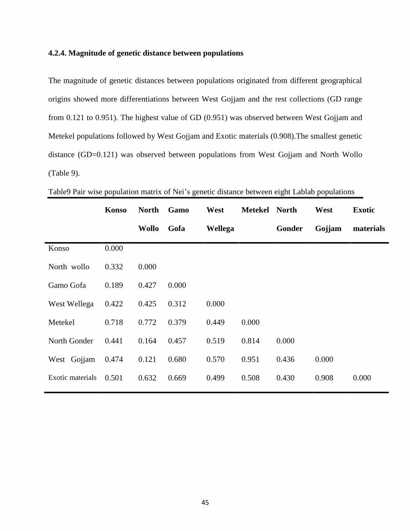
45
4.2.4. Magnitude of genetic distance between populations
The magnitude of genetic distances between populations originated from different geographical
origins showed more differentiations between West Gojjam and the rest collections (GD range
from 0.121 to 0.951). The highest value of GD (0.951) was observed between West Gojjam and
Metekel populations followed by West Gojjam and Exotic materials (0.908).The smallest genetic
distance (GD=0.121) was observed between populations from West Gojjam and North Wollo
(Table 9).
Table9 Pair wise population matrix of Nei’s genetic distance between eight Lablab populations
Konso North
Wollo
Gamo
Gofa
West
Wellega
Metekel North
Gonder
West
Gojjam
Exotic
materials
Konso 0.000
North wollo 0.332 0.000
Gamo Gofa 0.189 0.427 0.000
West Wellega 0.422 0.425 0.312 0.000
Metekel 0.718 0.772 0.379 0.449 0.000
North Gonder 0.441 0.164 0.457 0.519 0.814 0.000
West Gojjam 0.474 0.121 0.680 0.570 0.951 0.436 0.000
Exotic materials 0.501 0.632 0.669 0.499 0.508 0.430 0.908 0.000

46
4.2.5 Genetic interrelationships between Lablab accessions
The dendogram of cluster analysis based on neighbor-joining algorithm using the un-weighted
pair group method (UWPGM) categorized the 91 Lablab accessions into three major clusters
consisting of 48%, 33% and19 % of the accessions in cluster I, II, and III, respectively forming
different sub-clusters (Fig. 11).Eighty percent of Exotic materials were grouped together in
cluster one but in separate sub-clusters. The first cluster mostly composed of accessions from all
populations. The second cluster contained accessions mainly from West Gojjam, North Wollo
and North Gondar. It was observed that accessions from geographically nearest populations of
North Wollo, West Gojjam and North Gonder constitute more than 80% of the total accessions in
the group, and in the third cluster comprised almost entirely Konso accessions (88%).

47
Figure 11 NJ dendrogram of 91 accessions
KEY
____ Konso
____North Wollo
____Gamo Gofa
____West Wellega
____Metekel
____North Gonder
_____West Gojjam
_____Exotic materials
C3
C2
C1

48
4.2.6. Principal coordinate analysis (PCOA)
PCoA revealed that the first three coordinates explain 22.55 % of the genetic variation. The first,
second, and third principal coordinates, respectively explained about 9.04 %, 6.78 % and 6.36 %
of the gross variation, respectively (Table 10).
The PCoA analysis displayed in (Fig. 12) showed that accessions from different collection sites
were clustered together confirming the result of NJ cluster analysis.
Table 10 Percentage of variation explained by the first three principal components using 15 SSR
markers across 91 genotypes
Axis 1 2 3
Individual %
9.04 6.78 6.36
Cumulative %
9.40 16.18
22.55

49
Figure 12 PCoA of 91 accessions and eight populations of Lablab using 15 SSR markers
4.2.7. Population structure
The STRUCTURE analysis divided the Lablab accessions into four genetic clusters. The four
groups were determined by Bayesian algorithm implemented in the software STRUCTURE. The
algorithm allows estimating the true number of clusters (K) in populations of the study. Based on
the true number of cluster (K) suggested by Evanno et al. (2005), the real structure showing a
clear peak of the populations was set at K = 4 (Fig. 13). It means that K = 4 found to be the most
likely number of clusters to divide the 91 accessions in to four (Fig. 14). Based on this value,
Clumpak result (bar plot) showed wide admixtures and hence there was no clear geographic
origin-based structuring of populations (Fig.14).
12
3
4
5
6
7
8 9
10
11
12
13
14
15
16
17
18 19
20
21
2223
24
25
26
27
28
2930
3132 33
343536
37
38
39
40
414243
4445
46
49
50
51
52 53
54
63
6769
5556
57
58
65
70
72
75
91
82
6264
66
68
73
77 74
76
4779
83
48
59
6080
81
61
71
788485
868788
89
90
Co
ord
. 2
Coord. 1
Principal Coordinates (PCoA)
1
2
3
4
5
6
7
8
Konso
North Wollo
Gamo Gofa
West Wellega
Metekel
North Gondor
West Gojjam
Exotic materials

50
Figure 13 Results of the STRUCTURE analysis of 91 Lablab accessions: The highest peak at
K=4
Table 11The Evanno output table
K Reps Mean LnP(K) Stdev LnP(K) Ln'(K) |Ln''(K)| Delta K
1 20 -6249.630000 0.991596 — — —
2 20 -5863.860000 44.184808 385.770000 6.700000 0.151636
3 20 -5484.790000 31.307959 379.070000 81.985000 2.618663
4 20 -5187.705000 1.230950 297.085000 140.490000 114.131402
5 20 -5031.110000 4.262431 156.595000 28.885000 6.776650
6 20 -4903.400000 80.100102 127.710000 29.215000 0.364731
7 20 -4804.905000 56.571412 98.495000 13.395000 0.236780
8 20 -4693.015000 15.791413 111.890000 32.785000 2.076128
9 20 -4613.910000 7.784053 79.105000 4.470000 0.574251
10 20 -4539.275000 11.208590 74.635000 — —

51
Figure 14 Estimated population structure of 91Lablab accessions as revealed by 15 polymorphic
SSR markers for (K=4)

52
CHAPTER FIVE
5 DISCUSSION CONCLUSION AND RECOMMENDATIONS
5.1. DISCUSSION
5.1.1. Diversity of farmers’ varieties of Lablab in Konso zone
Landraces/ farmers’ variety are populations of a cultivated crop with a historical origin, distinct
identity, often genetically diverse and locally adapted, and associated with a set of farmers’
practices of seed selection and field management as well as with a farmers’ knowledge base
(Camacho-Villa et al., 2005).Farmers who cultivate local varieties of Lablab in the study zone
use morphological traits of seeds for identification and selection of varieties. For example, the
varieties called Okala tima, Okala ata and Okala abora were named based on their seed color
meaning red seeded, white seeded and black seeded, respectively in Konsogna languge (Konso
language). Similar results were reported by Tura Barekeet al. (2018) in Common bean in
Southern and Eastern Ethiopia use morphological traits of seeds for identification and selection
of farmers’ varieties. Based on names and descriptions given by farmers, six Lablab local
varieties were identified in the study area.
5.1.2. Cropping systems and management practice
In the study area, all Lablab varieties were grown as an intercrop cropping with sorghum, maize
and finger millet and grown as a sole crop in the margin of terracing and fence line. Konso
farming system utilizes a multiple cropping system which incorporates a combination of
different crops. This is probably because of Konso people are well known for their traditional
land management and conservation practices, intercropping of the crop with other cereal crops
can protect soil erosion and improve soil fertility. In this study, sorghum is the major

53
intercropped cereal (99%) and maize is the second most intercropped crop (89%) cereal with
Lablab in all surveyed areas of Konso. Likewise, Menfese Tadesse, (2010) in Konso people of
southern Ethiopia have been known for their indigenous intensive agricultural land management
and soil conservation practices.
5.1.3. Use of Lablab in the study area
Farmers used Lablab as food in the form of boiled grains (nifro). As the respondent said that, the
dry seeds are eaten as boiled grain (nifro) after prolonged cooking with several changes of water.
Nifro is the major food that the farmers used from seed of Lablab. Tefera Tolera (2006) and
Maasset al. (2010) reported that green pods, mature seeds and leaves are traditionally eaten as
vegetables in Africa, South and South-east Asia. The use of Lablab for food in this study seems
to vary considerably with other countries, as some uses reported from other countries were not
recorded in the study area.
The farmers of the study area also mentioned that the fodder of Lablab is very important for their
cattle production. This is because of Lablabis one of the most palatable legumes for animals
(Valenzuela and Smith, 2002). The leaf has crude protein of 21 to 38% and the seed contains 20
to 28% crude protein (Cook et al., 2005). Additionally, Lablab also plays a great role in
improving soil fertility and making it suitable for cereal crops such as sorghum, maize and finger
millet when grown as intercropping/mixed cropping. Similar report was mentioned by Kimani et
al. (2012), Lablab is a multipurpose legume crop used as a pulse crop for human consumption,
as a fodder crop for livestock, as a rotational and cover crop to improve soil fertility and soil
organic matter.

54
5.1.4. Gender and age roles in production and management of Lablab in the study
area
In the study area, most of the management practices/agronomic practices in the cropping of
Lablab were mostly done by both men and women adults. Both of them participate in hoeing,
planting, weeding, adding organic fertilizers, harvesting, threshing, and storage. Men and women
often work together in the field, but most activities are carried out by women. Male and female
children also participate in planting, weeding, harvesting, threshing and storage activities. This
indicates that the crop is well managed by the male and female adults within the study area. The
reason for this phenomenon is that ploughing and crop cultivation in Konso is done mainly by
hand hoeing; thereby resulting in a higher demand for household labor than in a farming system
using the ox plough method. Similar study conducted by Menfese Tadesse (2010) showed men
have relatively low work burdens than women with increasing work load during the peak
seasons. Women are engaged throughout the year in addition to their regular household
responsibilities. Similarly, studies conducted by Abayneh Feyso et al. (2019) in Konso on gender
roles in crop production have indicated that women play a great role than men on farm work
activities.
5.1.5. Planting month of Lablab in the study area
As both the key and general informants mentioned, planting of Lablab was done following the
start of rain from February to April. Based on the survey result, planting time of Lablab was
mainly from mid February to late March. The extension of planting time could be variability of
rainfall in Konso. According to key informants’ information, March was the main planting
season of the crop in Konso zone. Abayneh Feyso et al. (2019) have reported planting of crop in

55
Konso zone starts as soon as the main rains begin in February. This is because of the production
of cycle crop is entirely dependent on rainfall.
5.1.6. Production constraint of Lablab
Farmers are facing different constraints of Lablab production. As the farmers mentioned,
drought, shortage of land, insects and diseases are the most important constraints for Lablab
production. Even though they could not identify the names of the insects and diseases, the
descriptions they provided showed that bruchid beetles (storage pest), powdery mildew, aphids
and pod borers are the most important problems for farmers. The most serious pest causing
losses to stored Lablab is bruchid beetles, which also attack the crop in the field. Similar results
were reported by Ramesh and Byregowda (2016), biotic stresses, such as anthracnose, Lablab
yellow mosaic virus (LaYMV) diseases, pod borers (Heliothis armigera ,Adisura atkinsoni) and
bruchids (Callosobruchus theobrome), are major biotic production constraints in Lablab.
5.1.7. Genetic diversity study using SSR markers
Molecular characterization of plant genetic diversity and relationships using microsatellite
markers is promising because of their co-dominance and ability to reveal a high number of
alleles per polymorphic locus.
The 15 SSR loci used in this study were highly polymorphic, resulting in 95.59% polymorphisms
and highly effective in differentiation of 91Lablab accessions. The results also revealed 225
alleles across all the accessions. The number of alleles per locus varied from nine for Lpxu-009
to 21 for KTD255 and KTD272. The values recorded in the present study are different from
previous studies using SSRs markers on Lablab (Zhang et al., 2013; Robotham and Chapman,
2017; Keerthi et al., 2018). This study recorded higher total number of allele (225) as compared

56
to report of 133 alleles by Keerthiet al. (2018). Similarly, the mean number of alleles (14.80)
detected in this study was higher than the mean number of alleles reported by Zhang et al.
(2013), Robotham and Chapman (2017) and Keerthi et al.(2018).According to their report, the
mean number of alleles ranged from 2.65 to 7.4. The differences in the mean number of alleles
and total number of alleles between the present study and the previous studies could be attributed
to the genetic materials and the number of genotypes used for this study was different and the
genotypic difference of the tested genotypes may cause the difference. Likewise, the mean
number of effective alleles (4.75) and Shannon information index (1.60) were higher than the
previous study reported by Keerthi et al. (2018).
PIC value of the present study indicates the markers used in the study were highly informative
and availability of high allelic variation in the marker loci and their distribution within the
studied Lablab genotypes. The result also indicates the usefulness of the markers for further
genetic analysis such as genetic diversity, genetic linkage map construction and QTL mapping of
Lablab genotypes in the future. The 15 SSR markers used in this study were selected from
Zhang et al. (2013), Robotham and Chapman (2017) and Keerthi et al. (2018) studies based on
their high PIC values. The mean value of PIC was higher than that reported by Zhang et al.
(2013), Robotham and Chapman (2017) and Keerthi et al. (2018). The reason for this result may
be attributed to the differences in the genetic diversity of the tested Lablab accessions, the
number (sample size) of accessions used for this study. The major allele’s frequency across the
accessions ranged from 0.13 to 0.32. This result indicated that the SSR markers used in this
study are very informative, and can be used in genetic diversity studies and in marker assisted
breeding in Lablab.

57
Heterozygosity can be considered as a measure of the amount of genetic variation within
genotypes. This parameter indicates how much the variation exists in the population and how the
variation distributed across the alleles of analyzed markers. The observed heterozygosity (Ho) is
the proportion of heterozygous individual in population samples and expected heterozygosity
(He) is the probability of an individual being heterozygous in any locus (Hirpara and Gajera,
2018). The observed heterozygosity revealed low values in relation to expected hetrozygosity at
all markers, which showed high amount of homozygosity.The observed lower heterozygosity in
Lablab genotypes reflects a low level of diversity within Lablab accessions or low levels of out
crossing. Robotham and Chapman (2017) also reported very low observed heterozygosity
(0.205) suggesting the inbreeding index characteristic of a minimum out crossing species. All of
the markers (100%) exhibited significant deviations from Hardy-Weinberg equilibrium between
observed and expected heterozygosity in which all of them showed excess heterozygosity that
led to a significant deviation from HWE across all populations. Such excess heterozygosity is
expected in sexually reproducing organisms that can maintain their heterozygosity through
sexual recombination. The average genetic diversity (0.86) and expected heterozygosity (0.75)
detected among the 91 Lablab accessions showed high levels of variation within the studied
Lablab populations.
5.1.8. Genetic relationship among populations
The high genetic variation observed within the tested Konso and West Wellega accessions could
be used as a potential source of important traits in the future Lablab breeding programs as the
private alleles provide a unique genetic variability in certain loci (Kalinowski, 2005).

58
5.1.9. Genetic distance between populations of Lablab
Pairwise comparison of Nei’s unbiased genetic distance among the eight populations ranged
from 0.121 between West Gojjam and North Wollo populations to 0.951 between West Gojjam
and Metekel populations. Metekel populations have larger genetic distance between the
population of North Gondar, West Gojjam and North Wollo. This could be because of low
genetic material exchange between the populations. Low genetic distances were also observed
between populations of North Gondar and North Wollo (0.164) and Konso and Gamo Gofa
(0.189). The low value of genetic distance indicates high frequency of identical alleles among
accessions, thus leads genetic homogeneity. This could be attributed to the proximity of these
geographical regions; hence there could be higher chances of exchanging and sharing of seed
through agricultural systems and farmers
5.10. Analysis of molecular variance
A low level of variations was observed among populations (6%), while high levels of variation
were revealed within populations (94%). This low genetic differentiation among population may
be due to gene flow as a result of exchange of germplasm by farmers across populations which
are geographically close to each other. This leads to an increase in the distribution of gene
among different populations. Similarly, Kimani et al. (2012) reported 99% variation within and
1% variation among Lablab populations using amplified fragment length polymorphism (AFLP)
markers. Kamotho et al. (2016)reported 85 % of genetic variation within populations and 15%
among populations for the tested Kenyan Lablab accessions using SSR markers. The low level of
genetic variability among Lablab populations may be as a result of gene flow (introduction and
migration of alleles or genotypes) from one population to another through seed exchange.

59
The study also showed the presence of moderate genetic differentiation among Lablab
populations (FST= 0.061). The magnitude among and within population differentiation was
quantified using F-statistics (Fit, Fis and Fst) also known as fixation indices (Wright, 1951).
Fixation index (Fst) is a measure of population differentiation due to genetic structure.
According to Wright (1951), Fst value ranges from 0 to 0.05 is considered as low, 0.05 to 0.15
moderate, and 0.15 to 0.25 large and greater than 0.25 indicate very large genetic
differentiations. A low level of genetic differentiation among populations could be indicative of a
high gene flow (Nm = 3.280).According to Slatkin (1985) and Waples (1987), Nm values
grouped into three categories: Nm > 1.00 high, 0.25-0.99 intermediate and 0.000 – 0.249 low.
Therefore, the high Nm value of 3.280 observed in this study indicates high gene flow among
populations which will agree with the AMOVA result showing low variation among the
populations.
5.11. Cluster analysis and relationship among accessions
The dendogram of cluster analysis based on neighbor-joining algorithm using UWPGM
categorized the 91 Lablab accessions into three main clusters (I, II, and II) by forming different
sub groups. Zhanget al. (2013)clustered 24 Lablab accessions in to two clusters using 11 EST-
SSR markers. The differences might be due to the number and type of accessions used for the
study. The clustering model showed the existence of weak relationships between the pattern of
genetic diversity and geographical origins of collections. Accessions collected from different
populations clustered together, which may be attributed to the existence of gene flow among
neighboring populations. Most of exotic materials were grouped with geographically distant
accessions in Cluster I. Accessions collected from Konso were also grouped in all clusters with
other geographically distant populations. This indicates accessions in one cluster might be

60
evolved from different lines of ancestry or independent events of evolutionary forces such as
genetic drift, mutation, migration, selection and germplasm exchange might be separated them
into related but different gene pools (Gemechu Keneni et al., 2012).
Moreover, this result is clearly reflected on the model based population genetic structure analysis
finding showing high potential of admixtures of gene across populations. It revealed the
existence of weak sub-structuring (K=4) of the eight populations of Lablab. This finding may
indicate germplasm exchange between farmers, leading to gene flow across adjoining
populations.
The overall grouping pattern of PCoA corresponds with the clustering dendrogram which
explains about conformity of results obtained from UPGMA analysis. The reason for these inter
mixing could be explained by gene flow from one area to the other.

61
5.2. CONCLUSION
The production and utilization of Lablab in different forms around Konso area implies that the
crop has tremendous potential to significantly contribute to both food and nutritional security of
the country. The indigenous knowledge to use intercropping type of cultivation practice in the
area may also contribute to nutritional diversity. The different biotic and abiotic constraints
affecting Lablab productivity are good indicators for the underutilization of the crop which
demands strong attention towards its genetic improvement and conservation in the future.
Successful molecular characterization of the crop helped to identify distinct grouping between
different Lablab accessions collected from different parts of Ethiopia. The abundance of different
alleles observed among the collections provides more evidence for novel alleles that can be
efficiently exploited through future breeding program for the trait of interest. The existence of
relatively higher genetic diversity in Konso and West Wellega collections also reveals that these
areas could be considered as hot spot for genetic diversity as well as sources of desirable genes
for genetic improvement and conservation. The results create an insight to exploit this
underutilized genetic resource through integration of modern tools to the existing indigenous
knowledge. Indigenous knowledge on Lablab production and management has tremendous
contribution for the genetic improvement and better use of the crop.

62
5.3. RECOMMENDATIONS
The limited collection of farmers’ varieties of Lablab at the Ethiopian Biodiversity
Institute signals the need to mount more collection of germplasm and conservation work.
Further ethnobotanical studies with seed collection of farmers’ varieties should be
conducted particularly in areas not covered by this study in order to have a full
documentation of Lablab farmers’ varieties and indigenous knowledge held by farmers in
Ethiopia.
Further analysis should be done on the genetic diversity and population structure of
Lablab accessions by including additional collections from all over the country using
high resolution markers.
Germplasm from Konso and West Wellega showed relatively high level of genetic
diversity and should be the main target area for future collection and population
improvement.

63
REFERENCES
Abayneh Feyso, Selamawit Markos and Awoke Mensa (2018). Participatory Gender Analysis of
Sorghum Value Chain: the Case of Konso zone, Ethiopia Implication for Sorghum
Research Improvement. Am. Rese. J. Bus. Man. 4: 1-11.
Arif, I.A., Bakir, M.A., Khan, H.A., Al Farhan, A.H., Al Homaidan, A.A., Bahkali, A.H., Al
Sadoon, M. and Shobrak, M. (2010). A brief review of molecular techniques to assess
plant diversity. Int. J. Mol. Sci. 11: 2079-2096.
Barcaccia, G. (2010). Molecular markers for characterizing and conserving crop plant
germplasm.In: Molecular techniques in crop improvement, pp. 231-254 (Mohan, S.
Jain and Brar D.S. (eds). Springer, Dordrecht.
Botstein, D., White, R.L., Skolnick, M. and Davis, R.W. (1980). Construction of a genetic
linkage map in man using restriction fragment length polymorphisms. Am. J. Hum.
Genet. 32:314.
Byregowda, M., Girish, G., Ramesh, S., Mahadevu, P., and Keerthi, C. (2015). Descriptors of
Lablab purpureus. J. food legu. 28: 203-214.
Camacho Villa, T.C., Maxted, N., Scholten, M. and Ford-Lloyd, B. (2005). Defining and
identifying crop landraces. Plant Genet. Resour. 3: 373–384.
Cook, B.G., Pengelly, B.C., Brown, S.D., Donnelly, J.L., Eagles, D.A., Franco, M.A., Hanson,
J., Mullen, B.F., Partridge, I.J., Peters, M. and Schultze-Kraft, R. (2005). Tropical
Forages: an interactive selection tool. CSIRO, DPI and F, CIAT, ILRI publisher,
Brisbane, Australia.

64
Cotton, C.M. (1996). Ethnobotany: Principles and Applications. John Wiley and Sons,
Chichester, England, pp. 347.
D’Souza, M.R. and Devaraj, V.R. (2010). Biochemical responses of Hyacinth bean (Lablab
purpureus) to salinity stress. Acta Physiol. Plant.32:341-353.
Duke J.A., Kretschmer A.E. Jr., Reed C.F. and Weder J.K.P. (1981). Lablab purpureus
(L.)Sweet.In: Handbook of Legumes of World Economic Importance, pp. 102–106
(Duke J.A. (ed.). Plenum Press, New York, USA and London, UK.
Dwivedi, S.L., Ceccarelli, S., Blair, M.W., Upadhyaya, H.D., Are, A.K. and Ortiz, R. (2016).
Landrace germplasm for improving yield and abiotic stress adaptation. Trends Plant
Sci. 21:31-42.
Earl Dent A. and vonHoldt Bridgett M. (2012).STRUCTURE HARVESTER: a website and
program for visualizing STRUCTURE output and implementing the Evanno
method.Conserv.Genet. Resour. 4: 359-361
EBI. (Ethiopia biodiversity institute) (2012). Ethiopia: third country report on the state of plant
genetic resource for food and agriculture Institute of Biodiversity Conservation, Addis
Ababa, Ethiopia Jaccard, P. 1908.
Edwards, S., Mesfin, Tadesse and Hedberg I. (1995).Flora of Ethiopia and Eritrea, the National
Herbarium, Addis Ababa University, Addis Ababa and Department of Systematic
Botany, Uppsala University, Uppsala.
Evanno, G., Regnaut, S., Goudet, J. (2005). Detecting the number of clusters of individuals using
the software STRUCTURE: a simulation study. Mol. Ecol. 14: 2611-2620.

65
Gemechu Keneni, Endashaw Bekele, MuhammadImtiaz, Kifle Dagne, Emana Getu, and Fassil
Assefa (2012). Genetic diversity and population structure of Ethiopian chickpea (Cicer
arietinum L.) germplasm accessions from different geographical origins as revealed by
microsatellite markers. Plant Mol. Biol. Rep.30:654-665.
Gilbert, J.E., Lewis, R.V., Wilkinson, M.J. and Caligari, P.D.S. (1999). Developing an
appropriate strategy to assess genetic variability in plant germplasm collections. Theor. Appl.
Genet. 98: 1125-1131
.Gonçalves, L.S.A., Rodrigues, R., do Amaral Junior, A.T., Karasawa, M. and Sudré, C.P.
(2009). Heirloom tomato gene bank: assessing genetic divergence based on
morphological, agronomic and molecular data using a Ward-modified location
model. Genet. Mol. Res. 8: 364-374.
Hirpara, D.G. and Gajera, H.P. (2018).Molecular heterozygosity and genetic exploitations of
Trichoderma inter-fusants enhancing tolerance to fungicides and mycoparasitism
against Sclerotium rolfsii Sacc. Infect. Genet.Evol. 66:26-36.
Kalinowski, S. T. (2005). HP-RARE 1.0: A computer program for performing rarefaction on
measures of allelic richness. Mol. Ecol. Notes, 5:187–189.
Kamotho, G. N., Kinyua, M. G., Muasya, R. M., Gichuki, S. T. and Wanjala, B. W. (2016).
Assessment of genetic diversity of kenyan dolichos bean ( Lablab purpureus (L.)
sweet ) using simple sequence repeat markers. Int. J. Agric. Envi. Biores.1: 26–43.

66
Kimani E.N., Wachira F.N. and Kinyua M.G. (2012) Molecular diversity of Kenyan Lablab
(Lablab purpureus (L.) Sweet) accessions using amplified fragment length
polymorphism markers. Am. J. Plant Sci. 3: 313-321
Kopelman N. M., Mayzel J., Jakobsson M., Rosenberg N. A. and Mayrose I. (2015).
CLUMPAK: a program for identifying clustering modes and packaging population
structure inferences across K. Mol. Eco.l Res. 15:1179–1191.
Kukade, S. A., and Tidke, J. A. (2014). Reproductive biology of Lablab purpureus (L.) Sweet
Fabaceae. Indian J. Plant Sci.3:22–25.
Kusse Haile, Jema Haji and Bosena Tegegne(2018).Technical efficiency of sorghum production:
The case of smallholder farmers in Konso District, Southern Ethiopia. J. Agric.
Dev. 3:1-15.
Liu K. J. and Muse S. V. (2005). Power Marker: an integrated analysis environment for genetic
marker analysis.Bioinformatics.21:2128–9.
Liu, C.J. (1996). Genetic diversity and relationships among Lablab purpureus genotypes
evaluated using RAPD as markers. Euphytica 90:115-119.
Maass B.L. (2016) Origin, domestication and global dispersal of Lablab purpureus (L.) Sweet
Fabaceae: current understanding. Legume Persp.13:5–8
Maass, B.L., Jamnadass, R.H., Hanson, J. and Pengelly, B.C. (2005): Determining Sources of
Diversity in Cultivated and Wild Lablab purpureus Related to Provenance of
Germplasm by using Amplified Fragment Length Polymorphism. Genet. Resour. Crop
Evol.52: 683-695.

67
Maass, B.L., Knox, M.R., Venkatesha, S.C. Angessa, T.T., Ramme, S. and Pengelly, B.C.,
(2010). Lablab purpureus-A crop lost for Africa?. Trop Plant Biol. 3:123-135
Martin, G.J. (1995). Ethnobotany: A method Manual. Chapman and Hall, London. pp. 265-270.
Mittal, N. and Dubey, A. (2009). Microsatellite markers - A new practice of DNA based markers
in molecular genetics. Pharmacogn Rev.3: 235-246
Muthusamy, S., Kanagarajan, S and Ponnusamy, S. (2008). Efficiency of RAPD and ISSR
markers system in assessing genetic variation of rice bean (Vigna umbellata)
landraces.Electronic J. Biotech.11: 32-41.
Nadeem, M.A., Nawaz, M.A., Shahid, M.Q., Doğan, Y., Comertpay, G., Yıldız, M., Hatipoğlu,
R., Ahmad, F., Alsaleh, A., Labhane, N. and Özkan, H. (2018). DNA molecular
markers in plant breeding: current status and recent advancements in genomic
selection and genome editing. Biotechnol. Equip. 32:261-285.
Nei, M. (1978).Estimation of average heterozygosity and genetic distance from a small number
of individuals.Genetics89: 583-590.
Park, Y., Lee, J. and Kim, N. (2009). Simple sequences repeat polymorphisms (SSRPs) for
evaluation of molecular diversity and germplasm classification of minor crops.
Molecules14: 4546-4569.
Pavel, A.B. and Vasile, C.I. (2012). PyElph-a software tool for gel images analysis and
phylogenetics. BMC bioinformatics 13:1-6

68
Pengelly, B.C. and Maass, B.L. (2001). Lablab purpureus (L.)Sweet–diversity, potential use and
determination of a core collection of this multi-purpose tropical legume. Genet.
Resour. Crop Evol. 48:261-272.
Perrier, X. and Jacquemoud-Collet, J.P. (2006).DARwin software: Dissimilarity analysis and
representation for windows. Website http://darwin.cirad. fr/darwin [accessed 1 March
2013].
Pritchard J. K., Stephens M. and Donnelly P. (2000).Inference of population structure using
multi-locus genotype data.Genetics155: 945–59.
Rabouam, C., Comes, A.M., Bretagnolle, V., Humbert, J.F., Periquet, G. and Bigot, Y. (1999).
Features of DNA fragments obtained by random amplified polymorphic DNA (RAPD)
assays. Mol. Ecol.8:493-503.
Rai, N., Kumar, A., Singh, P.K., Singh, M., Datta, D. and Rai, M. (2010). Genetic relationship
among Hyacinth bean (Lablab purpureus) genotypes cultivars from different races
based on quantitative traits and random amplified polymorphic DNA marker. Afr. J.
Biotechnol. 9:137-144
Ramesh, S. and Byregowda, M. (2016). Lablab (Lablab Purpureus (L.)Sweet, var. lignosus)
genetics and breeding - present status and future prospects.Mysore J. Agric. Sci.
50:481–500
Robotham, O. and Chapman, M. (2017). Population genetic analysis of hyacinth bean (Lablab
purpureus (L.) Sweet, Leguminosae) indicates an East African origin and variation in
drought tolerance. Genet. Resour. Crop Evol.64:139-148

69
She, C.W. and Jiang, X.H.(2015). Karyotype analysis of Lablab purpureus (L.) Sweet using
fluorochrome banding and fluorescence in situ hybridisation with rDNA probes.
Czech. J. Genet. Plant Breed.51:110–116
Sheahan, C.M. (2012). Plant guide for Lablab (Lablab purpureus), USDA-Natural Resources
Conservation Service, Cape May Plant Materials Center.
Shivachi, A., Kinyua, M.G., Kiplagat, K.O., Kimurto, P.K. and Towett, B.K. (2012).Cooking
time and sensory evaluation of selected Lablab purpureus genotypes. Afr. J. Food Sci.
Technol. 3:155-159.
Slatkin, M. (1985).Rare alleles as indicators of gene flow.Evolution.39: 53-65.
Staub, J.E., Serquen, F.C. and Gupta, M. (1996). Genetic markers, map construction, and their
application in plant breeding. Hort. Science 31:729-741.
Sumarani, G., Pillai, S., Harisankar, P. and Sundaresan, S. (2004). Isozyme analysis of
indigenous cassava germplasm for identification of duplicates.Genet. Resour. Crop
Evol.51: 205-209
Tadesse Abate (2017). Application of genetic markers for Plant genetic diversity study.J. Nat.
Sci.Rese.7: 31-37
Tadesse Menfese (2010). Living with Adversity and Vulnerability: Adaptive Strategies and the
Role of Trees in Konso, Southern Ethiopia.Doctoral Thesis, Swedish University of
Agricultural Sciences, Uppsala.

70
Tefera Tolera (2006): Towards improved vegetable use and conservation of cowpea (Vigna
unguiculata) and Lablab (Lablab purpureus): agronomic and participatory evaluation
in northeastern Tanzania and genetic diversity study. Cuvillier Verlag, Goettingen, p.
214
Tesfaye Awas (2007). Plant Diversity in Western Ethiopia: Ecology, Ethnobotany and Conserva
tion. Dissertation presented for the degree of Doctoral Philosophy, University of Osol,
Norway.
Treuren, R., Bas, N., Goossens, P., Jansen, J. and Soest, L. (2005). Genetic diversity in perennial
ryegrass and white clover.Mol. Ecol.14: 39-52.
Tuomisto, H. (2010). A diversity of beta diversities: straightening up a concept gone awry.
Defining beta diversity as a function of alpha and gamma diversity.Ecography 33:
2−22.
Tura Bareke, Zemede Asfaw, Zerihun Woldu, Beth, M. and Birhanu Amssalu (2018).Diversity
of common bean (Phaseolus vulgaris(L.), Fabaceae) landraces in parts of southern and
eastern Ethiopia. Adv. Plants Agric. Res. 8:449-457.
Vaijayanthi, P.V. and Ramesh, S. (2019). LablabGenetics, Breeding and Genomics.In:Advances
in Plant Breeding Strategies: Legumes, pp. 287-318 (Al-Khayri, J.M., Jain, S.M. and
Johnson, D.V., eds) Springer Nature, Switzerland.
Valenzuela, H.and Smith, J. (2002). Sustainable agriculture green manure crops.SA-GM-7.
Cooperative Extension Service, College of Tropical Agriculture and Human
Resources, University of Hawaii at Manoa.

71
Verdcourt, B. (1970): Lablab Adans. In: Studies in the Leguminosae- Papilionoideae of the
‘Flora of Tropical East Africa’: IV. Kew Bull 24: 409-411.
Verdcourt, B. (1971). Studies in the Leguminosae-Papilionoïdeae for the'Flora of Tropical East
Africa': V. Kew Bulletin, pp.65-169.
Verdcourt, B. (1979): Lablab. In: A manual of New Guinea legumes. Botany Bulletin 11: 537.
Vos, P., Hogers, R., Bleeker, M., Reijans, M., Lee, T.V.D., Hornes, M., Friters, A., Pot, J.,
Paleman, J., Kuiper, M. and Zabeau, M. (1995). AFLP: a new technique for DNA
fingerprinting. J. Nucleic Acids 23:4407-4414.
Wang, H., Wu, Z., Lu , J., Shi, N., Zhao,Y., Zhang, Z. and Liu, J. (2009). Molecular diversity
and relationships among Cymbidium goeringii cultivars based on inter simple
sequence repeat (ISSR) markers. Genetica136: 391–399.
Waples, R.S. (1987). A multi species approach to the analysis of gene flow in marine shore
fishes.Evolution41: 385-400.
Weising, K., Nybom, H., Wolff, K. and Kahl, G. (2005). DNA Fingerprinting in Plants:
Principles, Methods, and Applications Second edition. Taylor and Francis Group, CRS
Press, New York.
White, H. and Peakall, R. (2015). GENALEX 6.502: Genetic analysis in Excel. Population
genetic software for teaching and research.Mol. Ecol. Notes. 6: 288-295
Whittaker,R.H. (1960).Vegetation of the Siskiyou Mountains, Oregon and California. Ecological
monographs 30: 279-338.

72
Wright, S. (1951). The genetic structure of populations. Annal Eugenics15: 323-354.
Yoseph Beyene (2005). Genetic analysis of traditional Ethiopian highland maize (Zea mays L.)
using molecular markers and morphological traits: implication for breeding and
conservation. PhD Dissertation, University of Pretoria, Pretoria
Zeven, A.C. (1980). Landraces: a review of definitions and classifications. Euphytica 104:127-
139.
Zhang, G., Xu, S., Mao, W., Gong, Y. and Hu, Q. (2013). Development of EST-SSR markers to
study genetic diversity in hyacinth bean (Lablab purpureus( L.). Plant OMICS, 6:295–
301.
.

73
APPENDICES
Appendix 1 Structured interview and informed oral consent
“Hello, first I will introduce myself; my name is Solomon Tamiru and I am a student at Addis
Ababa University in the Institute of Biotechnology and this is my colleague who is assisting me
as a local guide and translator. We are conducting a study of the crop Lablab as part of my
education at the university.” The purpose of this study is to identify different types of Lablab and
to understand their uses and management by farmers. With your permission, I would like to ask
you questions about Lablab. Of course, your participation is entirely voluntary. These interviews
require less than one hour. I do not anticipate that the interview will pose any risks to you.
Because I am a student, I cannot pay you.
I hope that my research will benefit farmers in Ethiopia by promoting the diversity of Lablab. If
you agree to an interview, you do not have to answer all of my questions, and you can tell me at
any time if you would like to stop. I would record your answers to my questions using my cell
phone and my notebook. I would include this information in my thesis, and it would be shared
with other researchers who are interested in Lablab. Do you have any questions? In case you
have any questions in the future, here is my contact information. Solomon Tamiru phone number
+251910991535. Do you agree to participate in this study of the crop Lablab? If yes, proceed
with the interview. If no, thank the farmer and continue to the next randomly-selected household.

74
Section 1: Basic information
Date of interview: Start time of interview:
Name of interviewer:
Region: Zone:
Woreda/District: Kebele/Sub-District:
Latitude (in decimal degrees): Longitude (in decimal degrees):
Altitude (in meters):
Agro ecological classification
Random number of household from farmers’ association list:
Relative wealth on farmers’ association list: ☐ Low income ☐ Middle/High income
Section 2: General information about informant
Name of informant:
Language spoken by informant during interview: ☐ Amharic ☐ Other (specify): __________
Age (observed): ☐ 18 to 30 ☐ 30 to 45 ☐ 45 to 60 ☐ 60+
Gender (observed): ☐ Male ☐ Female
Is the informant the household head? ☐ Yes ☐ No
If no, household-head gender: ☐ Female-headed ☐ Male-headed

75
Section 3: Market access
How far is the closest market from your home? In minutes on foot
Do you go to any other larger market? ☐ Yes ☐ No
If yes, how far is this larger market from your home? In minutes (on foot)
How far is the nearest road with vehicle transport from your home? In minutes (on foot)
Section 4: Interspecific diversity of legume crops
Are you growing any legumes this year? ☐ Yes ☐ No
If yes, how many hectares.
Which legumes did you plant in 2010 E.C (Meskerem to Pagume)?
For each of the legumes you listed, how many hectares of land did you plant in 2010 E.C
(Meskerem to Pagume) including any areas under intercropping? Convert any local units to
hectares (e.g. 1 timad or qurt = 0.25 hectare).
Section 5: Use of Lablab (Lablab purpureus)
How do you use Lablab (Lablab purpureus)?
☐ Food ☐ Spice ☐ Medicine ☐ Fodder/Forage ☐ Fuel
☐ Market ☐ Bee forage ☐ Other (specify): ________
Section 6: Cropping practices
Do you rotate Lablab with other crops? ☐ Yes ☐ No
If yes, with which crops do you rotate Lablab?
If yes, how often do you plant Lablab within the crop sequence?
Do you intercrop Lablab with other crops? ☐ Yes ☐ No
If yes, with which crops do you plant Lablab in the same field?

76
Section 7: Intraspecific diversity of Lablab (Lablab purpureus)
Note: Be sure to include all varieties, including landraces and released/improved types.
What varieties of Lablab have you grown in the past three years (for the 2009, 2010, and 2011
harvests)?
Are there any other varieties that you have grown in the past, prior to 2009?
Are there any other varieties of Lablab grown by other farmers in your community, but not by
yourself?
Are there any other varieties of Lablab that you remember from a long time ago, or have heard
about from Elders, that are no longer grown by your community?
If you run out of a particular variety, whom would you ask to replenish your seeds? (Record
name as a potential key informant).
Section 8: Key attributes of varieties
Instructions: At the top of each column, write the names of all varieties harvested in 2009,
2010, and 2011. Use additional sheets if necessary
Question Variety 1 Variety 2 Variety 3 Variety 4
Local vernacular name of variety
Is this a traditional or a new variety?
Where did you first obtain this variety? (e.g. family,
neighbors*, DA, market, food aid, research center)
For how many years have you planted this variety?
Where do you plant this variety? (e.g. main fields,
field margins, home gardens, fence lines, other
places)
Are the places where you grow this variety rain fed,
irrigated, or both?

77
Do you plant this variety on soils with low,
moderate, and/or high fertility?
How many times per year do you sow this variety?
When do you usually sow this variety?
When do you usually harvest this variety?
Is this variety grown mainly for home use or mainly
for the market?
How many hectares of these varieties did you
harvest in 2009 E.C. and 2010 E.C., including area
under intercropping? Make sure you convert any
local units to hectares (e.g. 1 timad or qert = 0.25
hectare).
2010:
2009:
2010:
2009:
2010:
2009:
2010:
2009:
How much of this variety did you harvest in 2008
and 2007? Record with local units to be converted
later. Be sure to include the name of the units.
Later, go to a local market to determine the
conversion factor from local units to kilograms.
2010:
2009:
2010:
2009:
2010:
2009:
2010:
2009:
Based on your experience, was the yield for this
variety in 2010 and 2011 a very high yield, a high
yield, a medium yield, a low yield, or a very low
yield?
2010:
2009:
2010:
2009:
2010:
2009:
2010:
2009:
What is the current price of this variety at your
local market? (use farmer units)
* If a particular variety came from friends or family, ask for the name of the individual who
provided it as a potential key informant. Record that person’s name in your notebook.

78
Section 9: Rating of attributes for varieties of Lablab (Lablab purpureus)
Ask the informant to rate the varieties of Lablab (Lablab purpureus) planted for the 2009, 2010,
and 2011 harvests. This is NOT a ranking activity, so multiple varieties may receive the same
score.
Rating criteria and scale Var. 1 Var. 2 Var. 3 Var. 4 Var. 5
Local name (copied from previous pages)
Best yield this variety has ever given you (5=very
high, 4=high, 3=medium, 2=low, 1=very low)
Yield under drought conditions (5=very high,
4=high, 3=average, 2=low, 1=very low)
Yield when excessive rain causing water logging
(5=very high, 4=high, 3=average, 2=low, 1=very
low)
Yield when rainy season begins late (5=very high,
4=high, 3=average, 2=low, 1=very low)
Yield when rainy season ends early (5=very high,
4=high, 3=average, 2=low, 1=very low)
Resistance to frost (5=never affected by frost,
4=rarely affected by frost, 3=sometimes affected by
frost, 2=often affected by frost, 1=always affected
by frost)
Resistance to common diseases (5=never affected
by diseases, 4=rarely affected, 3=sometimes

79
affected, 2=often affected, 1=always affected by
diseases)
Tolerance to common insect pests (5=never
affected by insect pests, 4=rarely affected,
3=sometimes affected, 2=often affected, 1=always
affected)
Tendency for seeds to detach/shatter (5=seeds
never detach/shatter 4=rarely detach/shatter,
3=detach/shatter about half the time, 2=often
detach/shatter, 1=always detach/shatter)
Importance as food for the household (5=extremely
important, 4=very important, 3=somewhat
important, 2=not so important, 1=not at all
important)
Importance as a source of income (5=extremely
important, 4=very important, 3=somewhat
important, 2=not so important, 1=not at all
important)
Importance as fodder for livestock (5=extremely
important, 4=very important, 3=somewhat
important, 2=not so important, 1=not at all
important)
Effect on soil fertility (5=very positive effect on

80
soil fertility, 4=some positive effect, 3=no effect,
2=some negative effect, 1=very negative effect on
soil fertility)
Ease of harvesting (5=Very easy to harvest, 4=easy,
3=neither easy nor difficult, 2=somewhat difficult,
1=very difficult to harvest)
Ease of preparing as food (5=very easy to harvest,
4=easy, 3=neither easy nor difficult, 2=somewhat
difficult, 1=very difficult to harvest)
Taste (5=very good taste, 4=good taste, 3=neither
good nor bad taste, 2=bad taste, 1=very bad taste)

81
Section 10: Gender roles in production and management of Lablab (Lablab purpureus)
Which gender and age groups
live in your household
(including the respondent)?
☐ M-children
☐ F-children
☐ M-adults
☐ F-adults
☐ M-Elders
☐ F-Elders
☐ Yes
☐ No
When it comes to Lablab (Lablab purpureus), who within the family usually participates in the
following activities? Check any that apply.
Activity Gender and age groups* Is this true for all
varieties?*
Ploughing with animals
(mares)
☐ M-children
☐ F-children
☐ M-adults
☐ F-adults
☐ M-Elders
☐ F-Elders
☐ Yes
☐ No
Preparing the soil by hand
with a hoe (mekofer)
☐ M-children
☐ F-children
☐ M-adults
☐ F-adults
☐ M-Elders
☐ F-Elders
☐ Yes
☐ No
Leveling soil and removing
uprooted weeds (gulgualo)
☐ M-children
☐ F-children
☐ M-adults
☐ F-adults
☐ M-Elders
☐ F-Elders
☐ Yes
☐ No
Sowing (zer mezerat) ☐ M-children
☐ F-children
☐ M-adults
☐ F-adults
☐ M-Elders
☐ F-Elders
☐ Yes
☐ No
Weeding (marem) and
cultivation (kutkuato)
☐ M-children
☐ F-children
☐ M-adults
☐ F-adults
☐ M-Elders
☐ F-Elders
☐ Yes
☐ No
Fertilizer application
(madaberia, fig, kompost…)
☐ M-children
☐ F-children
☐ M-adults
☐ F-adults
☐ M-Elders
☐ F-Elders
☐ Yes
☐ No
Harvesting (mached ena ☐ M-children ☐ M-adults ☐ M-Elders ☐ Yes

82
mesebseb) ☐ F-children ☐ F-adults ☐ F-Elders ☐ No
Threshing (mewkat) ☐ M-children
☐ F-children
☐ M-adults
☐ F-adults
☐ M-Elders
☐ F-Elders
☐ Yes
☐ No
Storage (makemachet) ☐ M-children
☐ F-children
☐ M-adults
☐ F-adults
☐ M-Elders
☐ F-Elders
☐ Yes
☐ No
Marketing (meshet) ☐ M-children
☐ F-children
☐ M-adults
☐ F-adults
☐ M-Elders
☐ F-Elders
☐ Yes
☐ No
Seed selection (zer memret) ☐ M-children
☐ F-children
☐ M-adults
☐ F-adults
☐ M-Elders
☐ F-Elders
☐ Yes
☐ No
Food preparation (megib
mazegajet)
☐ M-children
☐ F-children
☐ M-adults
☐ F-adults
☐ M-Elders
☐ F-Elders
☐ Yes
☐ No
Collection of fodder for
animals (meno mesebsebe)
☐ M-children
☐ F-children
☐ M-adults
☐ F-adults
☐ M-Elders
☐ F-Elders
☐ Yes
☐ No
Other activity (specify): ☐ M-children
☐ F-children
☐ M-adults
☐ F-adults
☐ M-Elders
☐ F-Elders
☐Yes
☐ No
* Note: For this classification only, children are individuals 14 and younger, adults are ages 15
to 59, and Elders are 60 or older.
** Take detailed notes of any exceptions for particular varieties.
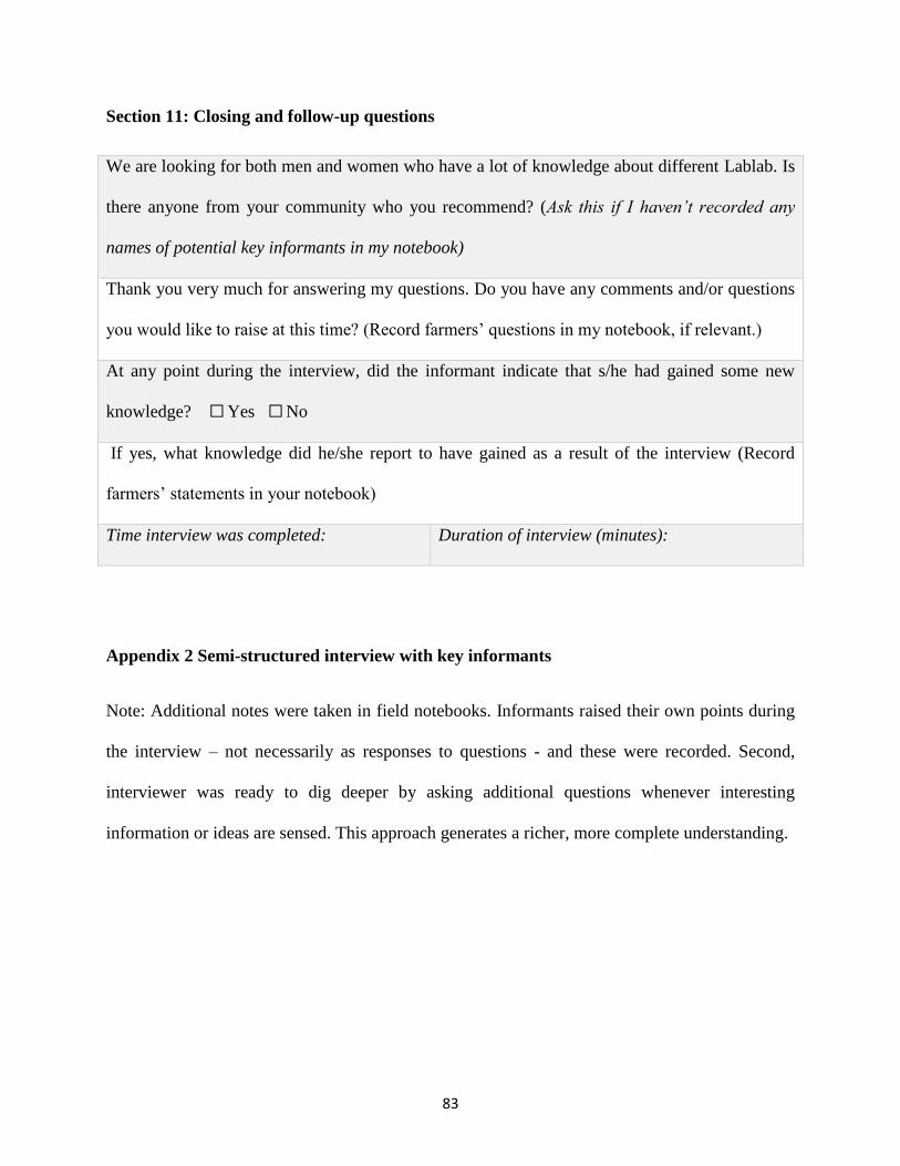
83
Section 11: Closing and follow-up questions
We are looking for both men and women who have a lot of knowledge about different Lablab. Is
there anyone from your community who you recommend? (Ask this if I haven’t recorded any
names of potential key informants in my notebook)
Thank you very much for answering my questions. Do you have any comments and/or questions
you would like to raise at this time? (Record farmers’ questions in my notebook, if relevant.)
At any point during the interview, did the informant indicate that s/he had gained some new
knowledge? ☐ Yes ☐ No
If yes, what knowledge did he/she report to have gained as a result of the interview (Record
farmers’ statements in your notebook)
Time interview was completed: Duration of interview (minutes):
Appendix 2 Semi-structured interview with key informants
Note: Additional notes were taken in field notebooks. Informants raised their own points during
the interview – not necessarily as responses to questions - and these were recorded. Second,
interviewer was ready to dig deeper by asking additional questions whenever interesting
information or ideas are sensed. This approach generates a richer, more complete understanding.

84
Section 1: Basic information about Key Informant
Date of interview: Start time of interview:
Name of interviewer:
Region: Zone:
Woreda/District: Kebele/Sub-District:
Language spoken during interview: ☐ Amharic ☐ Other (specify): ___________________
Name of informant:
Age (observed): ☐ 18 to 30 ☐ 30 to 45 ☐ 45 to 60 ☐ 60+
Gender (observed): ☐ Male ☐ Female
Section 2: Knowledge of varieties listed within the same kebeles
Compile a list of all of the varieties that have been mentioned by the general informants within
the same kebele. For each variety, ask the following questions of the key informant. Remember
to note if the key informant says that two or more local names refer to the same variety.
Are there any other varieties that you know that we can add to our list? You may include any that
you remember or have heard about from a long time ago, but are no longer planted in the kebele.
Names of varieties
(from ODK survey)
Have you heard of
this variety?
Is this variety planted
in this kebele?
Have you planted this
variety yourself?
1. ☐ Yes ☐ No ☐ Yes ☐ No ☐ Yes ☐ No
2.
☐ Yes ☐ No ☐ Yes ☐ No ☐ Yes ☐ No
3. ☐ Yes ☐ No ☐ Yes ☐ No ☐ Yes ☐ No
4. ☐ Yes ☐ No ☐ Yes ☐ No ☐ Yes ☐ No

85
Section 3: Attributes/characteristics of varieties
Instructions: Ask the key informants the following questions about each of the varieties with
which s/he is familiar. Record the information in your notebook. The following table is intended
to keep track of the questions you have asked.
Question V1 V2 V3 V4 V5 V6 V7 V8 V9 V10
What is the meaning of the local name? (e.g.
color, shape, nutritional quality, origin, etc.)
Are there alternative names for this variety?
How do you recognize this variety? How
does it differ from similar varieties? (By
appearance or other features?)
What are the ideal growing conditions for
this variety (e.g. amount and timing of
rainfall, sunlight, temperature)?
Characterize the soil types on which the
variety is planted.
What fraction of the farmers in your
community plants this variety? (e.g. almost
all, half, one out of ten)
Over the past 5 years, has this variety become
more commonly planted or less commonly
planted in your community?
If applicable…What is the main reason that
this variety is becoming more or less
common?

86
Section 4: Use of Lablab (Lablab purpureus) as food
What foods do you prepare using Lablab?
Note: Add a note if foods are of special cultural value. You may include foods that the key
informant does not prepare her/himself.
Name of food Which parts are used?
Which variety is preferred? Why is this variety
preferred?
*For example, color, taste, ease of preparation, etc
Section 5: Nutritional value of foods prepared with Lablab (Lablab purpureus)
Do any of the foods you prepare with Lablab have any special health benefits?
Name of food Health benefit Specific group
who use it or for
whom it is
recommended*?
Which variety
is preferred?
Why is this
variety preferred?
*For example: children, elderly, pregnant women, lactating women, sick people, people with
broken bones, people who have lost a lot of blood.
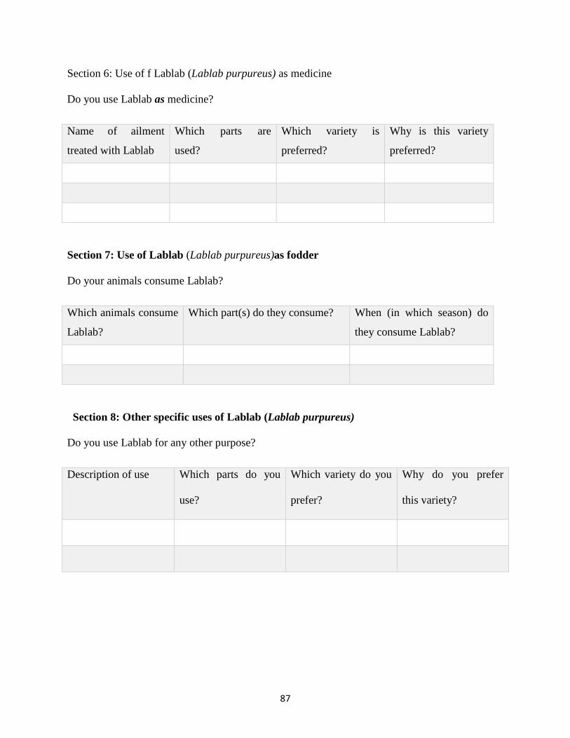
87
Section 6: Use of f Lablab (Lablab purpureus) as medicine
Do you use Lablab as medicine?
Name of ailment
treated with Lablab
Which parts are
used?
Which variety is
preferred?
Why is this variety
preferred?
Section 7: Use of Lablab (Lablab purpureus)as fodder
Do your animals consume Lablab?
Which animals consume
Lablab?
Which part(s) do they consume? When (in which season) do
they consume Lablab?
Section 8: Other specific uses of Lablab (Lablab purpureus)
Do you use Lablab for any other purpose?
Description of use Which parts do you
use?
Which variety do you
prefer?
Why do you prefer
this variety?

88
Section 9: Crop Management
1. Do the people in your community apply fertilizers to Lablab? Which fertilizers are used
(including manure, compost, crop residues)?
2. Do people in your community use pesticides or herbicides on Lablab?
3. What else do people in your community do to prevent and control pests, weeds, and
diseases affecting Lablab?
4. Are there any varieties of Lablab that produce more residues (stems, leaves, etc.) than
others?
5. What do people in your community do with the residues from Lablab? After the harvest?
6. Does anyone in your community ever use inoculants for Lablab?
7. How do people in your community store Lablab?
8. What are the major production constraints for Lablab in your community (e.g. weeds,
pests, diseases, drought, low fertility etc?)
Section 10: Closing and follow-up questions
I have asked all of the questions I had for you. Thank you very much for spending this time with
me and sharing your knowledge. Do you have any comments and/or questions you would like to
raise at this time? (Record farmers’ questions below)
(During the interview, did the informant indicate s/he had gained some new knowledge or some
kind of appreciation of what you are doing? ☐ Yes ☐ No)
If yes, what knowledge did he/she report to have gained as a result of the interview?
Time interview was completed: Duration of interview (in minutes):
Additional notes:
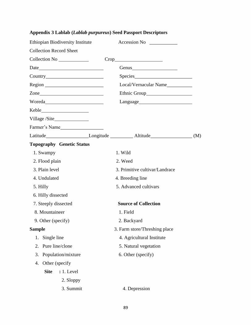
89
Appendix 3 Lablab (Lablab purpureus) Seed Passport Descriptors
Ethiopian Biodiversity Institute Accession No
Collection Record Sheet
Collection No Crop
Date Genus
Country Species
Region Local/Vernacular Name
Zone Ethnic Group
Woreda Language
Keble
Village /Site
Farmer’s Name
Latitude Longitude Altitude (M)
Topography Genetic Status
1. Swampy 1. Wild
2. Flood plain 2. Weed
3. Plain level 3. Primitive cultivar/Landrace
4. Undulated 4. Breeding line
5. Hilly 5. Advanced cultivars
6. Hilly dissected
7. Steeply dissected Source of Collection
8. Mountaineer 1. Field
9. Other (specify) 2. Backyard
Sample 3. Farm store/Threshing place
1. Single line 4. Agricultural Institute
2. Pure line/clone 5. Natural vegetation
3. Population/mixture 6. Other (specify)
4. Other (specify
Site : 1. Level
2. Sloppy
3. Summit 4. Depression

90
Soil Texture Nature of Samples
1. Sand 1. Seed
2. Sandy loam 2. Spikes
3. Loam 3. Pods
4. Clay loam 4. Cherry
5. Clay 5. Tuber
6. Silt 6. Rhizomes
7. Highly organic
8. Other (specify)
Herbarium Specimen Yes, No
Photographs Yes, No
Soil Color Sowing Month:
1. Black 1 2 3 4 5 6 7 8 9 10 11 12
2. Brown Early/Mid/Late
3. Orange Harvesting Month
4. Red 1 2 3 4 5 6 7 8 9 10 11 12
5. Yellow Early/Mid/Late
6. Other (specify)
Stoniness Origin of Seed
1. None 1. Local
2. Low 2. Elsewhere
3. Medium
4. Rocky Usage (specify)
Drainage Disease and Pests
1. Poor Note (Associated wild weedy species, crop,
2. Moderate local flora, disturbance factor)
3. Well drained
Shade Yes No
Remark
Collectors Name (s):

91
Appendix 4 List of the tested accessions and their geographical origins
code
Accession
Region
Zone
Woreda/Districts
Latitude
Longitude
Altitude
1 001 SNNPR Konso Konso special district 5° 20' 10.1142"
37° 24' 24.5232"
1638.2
2 002 SNNPR Konso Konso special district 5° 19' 49.8174"
37° 24' 23.9502"
1643.3
3 003 SNNPR Konso Konso special district 5° 20' 1.8342"
37° 25' 16.2582"
1583.1
4 004 SNNPR Konso Konso special district 5° 17' 28.4208"
37° 23' 46.7874"
1744.5
5 005 SNNPR Konso Konso special district 5° 20' 1.7226"
37° 25' 15.4914"
1586.6
6 006 SNNPR Konso Konso special district 5° 20' 3.2742"
37° 25' 13.278"
1619.8
7 007 SNNPR Konso Konso special district 5° 20' 3.1842"
37° 25' 14.9592"
1568.5
8 008 SNNPR Konso Konso special district 5° 17' 20.7132"
37° 21' 32.4828"
1842.8
9 009 SNNPR Konso Konso special district 5° 17' 19.518"
37° 21' 33.8826"
1864.5
10 010 SNNPR Konso Konso special district 5° 18' 51.2202"
37° 24' 30.7548"
1719.5
11 011 SNNPR Konso Konso special district 5° 17' 32.19"
37° 22' 39.684"
1855
12 012 SNNPR Konso Konso special district 5° 20' 7.7892"
37° 24' 31.5822"
1576
13 013 SNNPR Konso Konso special district 5° 17' 30.732"
37° 22' 39.8382"
1757
14 014 SNNPR Konso Konso special district 5° 17' 27.1392"
37° 23' 48.7788"
1735.4
15 015 SNNPR Konso Konso special district 5° 17' 28.6008"
37° 23' 46.0674"
1715
16 016 SNNPR Konso Konso special district 5° 17' 27.1062"
37° 23' 46.5534"
1488.3
17 017 SNNPR Konso Konso special district 5° 19' 49.944"
37° 24' 23.5332"
1644.3

92
18 018 SNNPR Konso Konso special district 5° 17' 29.0868"
37° 21' 32.58"
1901
19 019 SNNPR Konso Konso special district 5° 17' 20.9754"
37° 21' 32.0652"
1848
20 020 SNNPR Konso Konso special district 5° 20' 10.6362" 37° 24' 25.416" 1578
21 021 SNNPR Konso Konso special district 5° 18' 49.2474" 37° 24' 33.3714" 1614.9
22 022 SNNPR Konso Konso special district 5° 18' 51.2202" 37° 24' 30.7548" 1719.5
23 023 SNNPR Konso Konso special district 5° 18' 44.2548" 37° 24' 38.9874" 1533.9
24 024 SNNPR Konso Konso special district 5° 18' 51.1734" 37° 24' 31.1112" 1913.1
25 031 Amahara North Wollo Guba Lafto 11° 55' 27’’ 39° 29’ 47’’ 2025.4
26 032 Amahara North Wollo Guba Lafto
11° 53’ 27 ‘’
39° 29’ 47’’
2025.4m
27 033 Amahara NorthWollo Kobo 12° 0’ 39’’ 39° 37’ 25’’ 1613.8
28 034 Amahara NorthWollo Guba Lafto
11° 53' 27"
39° 29’ 47’’
2071m
29 035 Amahara NorthWollo Guba Lafto
11° 53’ 33’’
39° 29’ 46’’
1858.3m
30 036 Amahara NorthWollo Guba Lafto 11° 53’ 30’’
39° 29’ 37’’
2097.4m
31 037 Amahara NorthWollo Kobo 12° 10’ 00’’ 39° 38’ 00’’ 1630m
32 038 Amahara NorthWollo Guba lafto 11 43 00 39 35 00 1880
33 039 Amahara NorthWollo Habru 12° 0’ 39’’ 39° 37’ 25’’ 1613.8
34 040 Amahara NorthWollo Habru 11° 45 1
39° 36’ 50’’
1833.5m
35 041 Amahara NorthWollo Kobo 12° 8' 49''
39° 37’ 56’’
1474m
36 042 Amahara NorthWollo Habru 11° 39 43
39° 39’ 30’’
1610.3m
37 043 Amahara NorthWollo Guba lafto 11°49' 30"
39° 35’ 13’’
1870.7m
38 044 Amahara NorthWollo gubalafto 11 50 00 39 44 00 1875
39 045 Amahara NorthWollo Guba lafto 11° 53 42
39° 27’ 31’’
2214.1m
40 046 Amahara NorthWollo Guba lafto 11° 53' 33"
39° 29’ 46’’
1858.3m
41 047 Amahara NorthWollo Guba lafto 11° 53 42
39° 27’ 31’’
2242.9m
42 048 Amahara NorthWollo woldia 11 49 55 39 36 9 1919.8

93
43 049 Amahara NorthWollo kobo
12° 0 ' 36"
39° 37’ 31’’
1604.8m
44 050 Amahara NorthWollo kobo 12° 0' 41"
39° 37’ 27’’
1622.5 m
45 051 Amahara NorthWollo Habru 11° 40’ 26’’
39° 39 23
1617.2m
46 052 Amahara NorthWollo kobo 12° 0’ 41’’
39° 37’ 27’’
1622.5 m
47 060 SNNPR Gamogofa Arebaminch zuriya 6 2 19.7 37 33 25.2 1225
48 061 SNNPR Gamogofa Arebaminch zuriya 5o 51’ 57 ‘’ 37 o 28’ 41’’ 1116.5
49 062 SNNPR Gamogofa Arebaminch zuriya 5 o 51’ 58’’ 37 o 28’ 42’’ 1119
50 063 SNNPR Gamogofa Arebaminch zuriya 6o 2’ 5’’ 37o 34’ 34’’ 1196.3
51 064 SNNPR Gamogofa Arebaminch zuriya
52 065 SNNPR Gamogofa Arebaminch zuriya
53 211427 SNNPR Gamogofa 05° -25-00-N
37° -24-00-E
1440.00
54 212974 SNNP
Gamogofa 05° -14-00-N
37° -01-00-E
1580
55 211476
SNNP
Gamogofa
56 211413 Benishangul
and Gumuz
Metekel Mandura
57 240517 Benishangul
and Gumuz
Metekel Debate
58 211414 Benishangul
and Gumuz
Metekel Dangure
59 211556 Benishangul
and Gumuz
Metekel Mandura
60 240516
Benishangul
and Gumuz
Metekel Debate
61 240518
Benishangul
and Gumuz
Metekel Bulen
62 211415 Orimiaya West Wellega
63 211419
Orimiaya West Wellega
64 211420 Orimiaya West Wellega
65 211421 Orimiaya West Wellega
66 211425 Orimiaya West Wellega

94
67 211426 Orimiaya West Wellega
68 070 Orimiaya West Wellega Gimbi 9011’40’’ 35057’26’’ 1868
69 071 Orimiaya West Wellega Gimbi 9011’44’’ 35057’34’’ 1873.2
70 072 Orimiaya West Wellega Gimbi 35057’28’’ 35057’28’’ 1871.1
71 073 Orimiaya West Wellega Gimbi 9011’30’’ E35057’22’’ 1822.7
72 211406 Amahara North Gondor GONDAR ZURIA
12-37-00-N
37-28-00-E
NA
73 211407
Amahara North Gondor DEMBIA
12-25-00-N
37-19-00-E
1830.00
74 211408
Amahara North Gondor DEMBIA
12-25-00-N
37-19-00-E
1830.00
75 211422 Amahara North Gondor DEMBIA
12-25-00-N
37-19-00-E
1830.00
76 211423 Amahara North Gondor DEMBIA
12-25-00-N
37-19-00-E
1830.00
77 211409 Amahara West Gojjam BURE
10-42-00-N
37-04-00-E
2120.00
78 211410 Amahara west Gojjam BURE
10-42-00-N
37-04-00-E
2120.00
79 080 Amahara West Gojjam BURE
10 42 36 37 4 12 2102
80 081 Amahara West Gojjam BURE 10 42 36 37 4 12 2102
81 082 Amahara West Gojjam BURE
10 42 36 37 4 12 2102
82 10984 USA
83 6529 Mali
84 147 Australia
85 7379 Keneya
86 11614 Mali
87 14417 Keneya
88 14429 Keneya
89 14455 Keneya
90 14461 Kenaya
91 14487 Keneya

95
Appendix 5 Plant DNA Extraction Protocol for Diversity Array Technology (DArT)
BUFFER STOCK SOLUTIONS
EXTRACTION BUFFER STOCK
To make 500 ml:
0.35 M sorbitol 31.9 g sorbitol
0.1M TrisHCl pH 8.0 50 ml 1M TrisHCl pH 8.0 h
5 mM EDTA pH 8.0 5 ml 0.5 M EDTA pH 8.0
Fill up to 500 ml nuclease free water
LYSIS BUFFER STOCKTo make 500 ml:
0.2 M Tris HCl pH 8.0 100 ml 1M Tri HCl pH 8.0
0.05 M EDTA pH 8.0 50 ml 0.5 M EDTA pH 8.0
2M NaCl 200 ml 5 M NaCl
2% CTAB 10 g CTAB
Fill up to 500 ml with nuclease free water
SARCOSYL STOCK 5% (w/v)
FRESH BUFFER WORKING SOLUTION:
0.5 % (w/v) sodium di-sulfite (= sodium meta-bisulfite)
2 % (w/v) PVP-40 (K29-32) Sigma
Dissolve in required volume of extraction buffer stock;
Add same volume of lysis buffer stock and 0.4 volume of extraction (=lysis) buffer stock
of sarcosyl stock
For example to make 120 ml of working solution:

96
Add 0.6 g sodium di-sulfite (= sodium metabisulfite) and 2.4 g PVP-40 (K29-32) to 50 ml
extraction buffer stock and dissolve.
Add 50 ml lysis buffer stock and 20ml Sarcosyl stock
For example to make 30 ml:
Add 0.15 g sodiumdisulfite (= sodium metabisulfite) and 0.6 g PVP-40 (K29-32) to 12.5 ml
extraction buffer stock and dissolve; add 12.5 ml lysis buffer stock and 5 ml sarcosyl stock
*This buffer may settle into two layers on standing. Heat to 65ºC and shake immediately before
adding to extraction tubes.
PROTOCOL
For 2 ml Eppendorf tubes:
Aliquot 1 ml of freshly prepared preheated to 65ºC well mixed “fresh buffer solution”
and place tubes to the 65ºC incubator or water bath, (3,4dayes old “fresh buffer solution”
works fine)
Grind required amount (same across all samples) of plant material in mortar and pestle
under liquid nitrogen to fine powder,
Suspend powder in 1 ml “fresh buffer solution” kept at 65ºC (make sure there are no
clumps, vortex if necessary)
Incubate at 65ºC for 1 h (can extend for another 30 min), invert tubes in every 20
minutes or incubate with gentle shaking
Cool down for 5 min and add 1 ml of chloroform : isoamyl alcohol (24 : 1) mixture
mix well for 30 min
Spin 20 min for 10,000 g, RT

97
Transfer water phase to fresh tube, add same volume of ice cold isopropanol and invert
tube ~ 10 times, nucleic acids should become visible
Spin 30 min at 10,000 x g, RT,
Discard supernatant and wash pellet with 1 ml 70 % EtOH
Discard EtOH, dry pellet and dissolve in 100 µl of nuclease free water
Check DNA quality and quantity on 1% agarose gel
Appendix 6 Quality and quantity of Lablab genomic DNA, using Nano Drop Spectrophotometry

98
Appendix 7Samples of gel images showing the different sizes of PCR products of SSR markers
generated from lablab accessions
100
200
300
500

99
A, Intercropping of lablab with Sorghum in the study area, Konso zone
B, Interview with key informants (photo by Solomon, December, 2018)
Lablab seedlings grown in green house
A
B