Adhesive normal contact between flatpunch and a visco-elastic half-space in

Dugdale approximation

Julia RengshausenNovember 11, 2016

BACHELOR THESIS

Department of System Dynamics and Physics of FrictionTechnical University Berlin

Reviewer 1: Prof. Dr. rer. nat. Valentin PopovReviewer 2: Dr. Ing. Qiang Li

Eidestattliche Versicherung

Hiermit erklare ich, dass ich die vorliegende Arbeit selbststandig und eigenhandigsowie ohne unerlaubte fremde Hilfe und ausschließlich unter Verwendung deraufgefuhrten Quellen und Hilfsmittel angefertigt habe.Berlin, den...........................................................................Unterschrift

ii

Contents

1 Introduction 11.1 Method of Dimensionality Reduction . . . . . . . . . . . . . . 3

2 General Analysis 5

3 Closed Form Solutions for Certain System Specifications 113.1 Large α . . . . . . . . . . . . . . . . . . . . . . . . . . . . . . 123.2 Small α . . . . . . . . . . . . . . . . . . . . . . . . . . . . . . 133.3 Comparison and Approximation Error . . . . . . . . . . . . . 16

4 Limiting Cases of Material Behavior 174.1 Elastic Case . . . . . . . . . . . . . . . . . . . . . . . . . . . . 174.2 Viscous Case . . . . . . . . . . . . . . . . . . . . . . . . . . . 18

5 Conclusion 19

6 Symbols 20

References 21

iii

1 Introduction

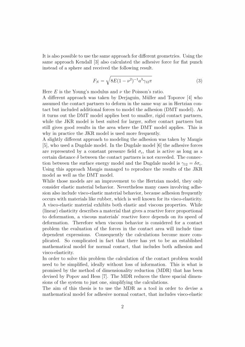
The study of contact problems has a long history and contact mechanics areneeded for many engineering applications e.g. brakes, bearings or electricalcontacts. The oldest and best known mathematical model of a normal contactwas published by Heinrich Hertz in 1882 [1]. In the Hertzian model a pres-sure field in the contact area is adjusted in a way so that the displacementsresulting from the pressure field correspond to the ones observed. Hertz as-sumes elastic materials and disregards any adhesion. This is sufficient formany applications involving materials that are only deformed in an elasticrange and don’t exhibit any viscous properties or adhesion. Nevertheless insome cases adhesion between the surfaces has a big enough impact to justifya more complicated model in order to include these effects. Generally theadhesion between two surfaces is described by the surface energy γ12 whichis defined as the energy needed to separate surfaces 1 and 2 (see Figure 1).

12

1

2

γ12

Figure 1: The surface energy γ12 is needed to divide surfaces 1 and 2

The contact model by Johnson, Kendall and Roberts (JKR model)[2] takesthis definition of adhesion and uses it to modify the Hertzian theory.Because Hertz had not included adhesion in his model, the Hertzian pressurefield does not produce any tensile loads. This is changed in the JKR modelwhere they modified the pressure field to include tensile terms. Then thetotal energy of the system UT is investigated. The total energy is comprisedof the adhesive surface energy and the potential energy arising from thedeformation. The system will be in equilibrium if

dUT

dt= 0 (1)

There are many equilibrium states, each with their corresponding contactradius a and normal force FN . The strongest of these normal forces will bethe force at detachment. For normal contact between a sphere of radius Rand an elastic half-space this is.

FN = −3

2γ12πR (2)

1

It is also possible to use the same approach for different geometries. Using thesame approach Kendall [3] also calculated the adhesive force for flat punchinstead of a sphere and received the following result.

FN =√

8E(1− ν2)−1a3γ12π (3)

Here E is the Young’s modulus and ν the Poisson’s ratio.A different approach was taken by Derjaguin, Muller and Toporov [4] whoassumed the contact partners to deform in the same way as in Hertzian con-tact but included additional forces to model the adhesion (DMT model). Asit turns out the DMT model applies best to smaller, rigid contact partners,while the JKR model is best suited for larger, softer contact partners butstill gives good results in the area where the DMT model applies. This iswhy in practice the JKR model is used more frequently.A slightly different approach to modeling the adhesion was taken by Maugis[5], who used a Dugdale model. In the Dugdale model [6] the adhesive forcesare represented by a constant pressure field σc, that is active as long as acertain distance δ between the contact partners is not exceeded. The connec-tion between the surface energy model and the Dugdale model is γ12 = δσc.Using this approach Maugis managed to reproduce the results of the JKRmodel as well as the DMT model.While those models are an improvement to the Hertzian model, they onlyconsider elastic material behavior. Nevertheless many cases involving adhe-sion also include visco-elastic material behavior, because adhesion frequentlyoccurs with materials like rubber, which is well known for its visco-elasticity.A visco-elastic material exhibits both elastic and viscous properties. While(linear) elasticity describes a material that gives a reactive force proportionalto deformation, a viscous materials’ reactive force depends on its speed ofdeformation. Therefore when viscous behavior is considered for a contactproblem the evaluation of the forces in the contact area will include timedependent expressions. Consequently the calculations become more com-plicated. So complicated in fact that there has yet to be an establishedmathematical model for normal contact, that includes both adhesion andvisco-elasticity.In order to solve this problem the calculation of the contact problem wouldneed to be simplified, ideally without loss of information. This is what ispromised by the method of dimensionality reduction (MDR) that has beendevised by Popov and Hess [7]. The MDR reduces the three spacial dimen-sions of the system to just one, simplifying the calculations.The aim of this thesis is to use the MDR as a tool in order to devise amathematical model for adhesive normal contact, that includes visco-elastic

2

material behavior, modeling the adhesion with a Dugdale potential. TheMDR has already been combined with a Dugdale potential for tangential ad-hesive contact with an elastic half-space by Popov and Dimaki [8] and someof their calculations in this respect also apply to the visco-elastic normalcontact. As the general case would be too expansive for a bachelor’s thesis,this general case will be reduced to a flat punch in adhesive contact with avisco-elastic half-space that is pulled off at a constant velocity.

1.1 Method of Dimensionality Reduction

The method of dimensionality reduction (MDR) is a method of simplifyingcontact problems. It was developed by Popov and Hess and described indepth in their 2013 book [7]. A comprehensive user’s manual was also pub-lished [9]. With the MDR normal and tangential contact problems can besimplified. It still gives exact solutions and is not an approximation tech-nique. The only restriction is that the shape of the punch needs to be rota-tionally symmetric.The simplification is done in two steps:First the continuum in contact with the punch is replaced by a one dimen-sional foundation. The makeup of this foundation depends on the propertiesof the continuum (see Figure 2).

Figure 2: Types of foundations: a) elastic materials are modeled as a seriesof springs, b) viscous materials are represented by dampers, c) visco-elastic

materials are modeled as a combination of a and b

The stiffness ∆k and damping coefficient ∆γ are

∆k = E∗∆x with1

E∗ =1− ν2

1

E1

+1− ν2

2

E2

(4)

and∆γ = 4η∆x (5)

where E is the Young’s modulus, ν the Poisson’s ratio and η the viscosity.Subscripts 1 and 2 refer to the two partners of contact.

3

The shape of the rotationally symmetric punch can be described by a func-tion of its profile f(r), where r is the radial coordinate. In the second stepof MDR f(r) is converted to a one dimensional profile g(x) via the transfor-mation

g(x) = |x||x|∫0

f ′(r)√x2 − r2

dr (6)

For returning to three dimensions the reverse transformation

f(r) =2

π

r∫0

g(x)√r2 − x2

dx (7)

is used.With these two steps a reduced system is defined, which is much easier tosolve than the original.

4

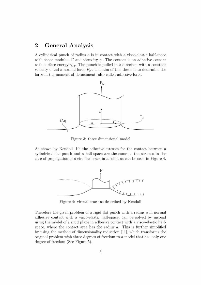
2 General Analysis

A cylindrical punch of radius a is in contact with a visco-elastic half-spacewith shear modulus G and viscosity η. The contact is an adhesive contactwith surface energy γ12. The punch is pulled in z-direction with a constantvelocity v and a normal force FN . The aim of this thesis is to determine theforce in the moment of detachment, also called adhesive force.

G,η r

z

a

FN

γ12

Figure 3: three dimensional model

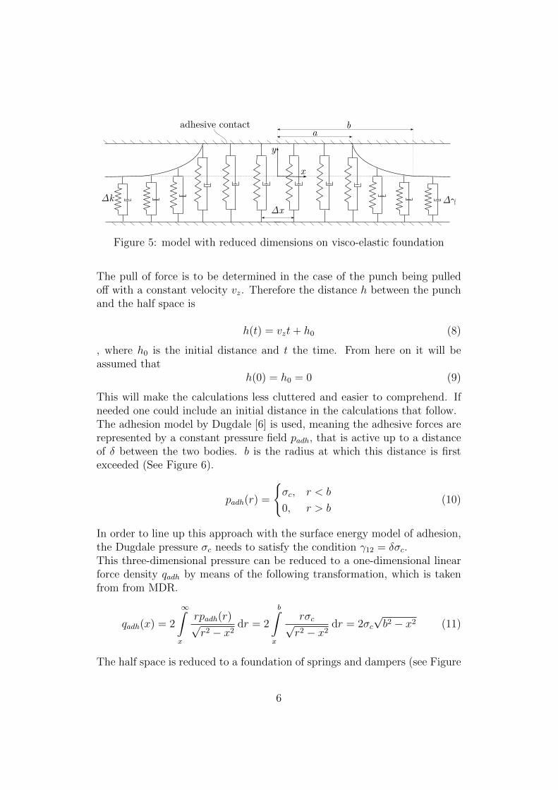
As shown by Kendall [10] the adhesive stresses for the contact between acylindrical flat punch and a half-space are the same as the stresses in thecase of propagation of a circular crack in a solid, as can be seen in Figure 4.

Figure 4: virtual crack as described by Kendall

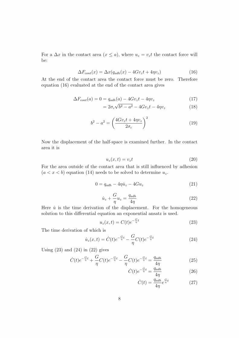
Therefore the given problem of a rigid flat punch with a radius a in normaladhesive contact with a visco-elastic half-space, can be solved by insteadusing the model of a rigid plane in adhesive contact with a visco-elastic half-space, where the contact area has the radius a. This is further simplifiedby using the method of dimensionality reduction [11], which transforms theoriginal problem with three degrees of freedom to a model that has only onedegree of freedom (See Figure 5).

5

Δk ΔγΔx

abadhesive contact

x

y

Figure 5: model with reduced dimensions on visco-elastic foundation

The pull of force is to be determined in the case of the punch being pulledoff with a constant velocity vz. Therefore the distance h between the punchand the half space is

h(t) = vzt+ h0 (8)

, where h0 is the initial distance and t the time. From here on it will beassumed that

h(0) = h0 = 0 (9)

This will make the calculations less cluttered and easier to comprehend. Ifneeded one could include an initial distance in the calculations that follow.The adhesion model by Dugdale [6] is used, meaning the adhesive forces arerepresented by a constant pressure field padh, that is active up to a distanceof δ between the two bodies. b is the radius at which this distance is firstexceeded (See Figure 6).

padh(r) =

{σc, r < b

0, r > b(10)

In order to line up this approach with the surface energy model of adhesion,the Dugdale pressure σc needs to satisfy the condition γ12 = δσc.This three-dimensional pressure can be reduced to a one-dimensional linearforce density qadh by means of the following transformation, which is takenfrom from MDR.

qadh(x) = 2

∞∫x

rpadh(r)√r2 − x2

dr = 2

b∫x

rσc√r2 − x2

dr = 2σc

√b2 − x2 (11)

The half space is reduced to a foundation of springs and dampers (see Figure

6

b0

σc

r

padh

Figure 6: A Dugdale Potential - The potential has the constant value of σc

before dropping to zero at a radius greater than b

5). The spring and damper constants are defined as

∆k = 4G∆x (12)

∆γ = 4η∆x (13)

, with G being the shear modulus and η the viscosity of the half-space.

Δk Δγ

uz

forces at nodeuzΔk Δγuz

.

qadhΔx

Figure 7: Equilibrium of forces for a ∆x. The adhesive force is constant,while the spring and damper forces depend on the displacement of the

surface of the half-space uz and its time derivation uz

The equilibrium of forces is evaluated for an arbitrary ∆x to determine thecontact force ∆Fcont (see Figure 7).

∆Fcont(x) = ∆x(qadh(x)−∆kuz +∆γuz) (14)

= ∆x(qadh(x)− 4Guz + 4ηuz) (15)

7

For a ∆x in the contact area (x ≤ a), where uz = vzt the contact force willbe:

∆Fcont(x) = ∆x(qadh(x)− 4Gvzt+ 4ηvz) (16)

At the end of the contact area the contact force must be zero. Thereforeequation (16) evaluated at the end of the contact area gives

∆Fcont(a) = 0 = qadh(a)− 4Gvzt− 4ηvz (17)

= 2σc

√b2 − a2 − 4Gvzt− 4ηvz (18)

b2 − a2 =

(4Gvzt+ 4ηvz

2σc

)2

(19)

Now the displacement of the half-space is examined further. In the contactarea it is

uz(x, t) = vzt (20)

For the area outside of the contact area that is still influenced by adhesion(a < x < b) equation (14) needs to be solved to determine uz.

0 = qadh − 4ηuz − 4Guz (21)

uz +G

ηuz =

qadh4η

(22)

Here u is the time derivation of the displacement. For the homogeneoussolution to this differential equation an exponential ansatz is used.

uz(x, t) = C(t)e−Gηt (23)

The time derivation of which is

uz(x, t) = C(t)e−Gηt − G

ηC(t)e−

Gηt (24)

Using (23) and (24) in (22) gives

C(t)e−Gηt +

G

ηC(t)e−

Gηt − G

ηC(t)e−

Gηt =

qadh4η

(25)

C(t)e−Gηt =

qadh4η

(26)

C(t) =qadh4η

eGηt (27)

8

Time integration of (27) yields

C(t) =qadh4G

eGηt + c (28)

And therefore (23) turns out to be

uz(x, t) =qadh4G

+ c e−Gηt (29)

With an initial value of uz(x, 0) = 0, which corresponds with the initial valueof h = 0, the constant c can be determined:

c = −qadh4G

(30)

This leads to the following expression for the displacement for a < x < b.

uz(x, t) =qadh4G

(1− e−

Gηt)=

2σc

√b2 − x2

4G

(1− e−

Gηt)

(31)

Therefore the complete displacement of the half-space in the reduced model,taken from (20) and (31), is

uz(x, t) =

{vzt, x < a2σc

√b2−x2

4G

(1− e−

Gηt), a < x < b

(32)

The case of x > b does not need to be considered, because outside the rangeof influence of the Dugdale potential there are no forces with influence onthe contact.

At this point a transformation back to the 3D-model is needed because sofar the calculations have taken place in the reduced MDR model. For thisthe following transformation is used

uz(r, t) =2

π

r∫0

uz(x, t)√r2 − x2

dx (33)

Using (33) on (32) the displacement at r = b can be determined

uz(b, t) =2

π

a∫0

vzt√b2 − x2

dx+2

π

b∫a

2σc

√b2 − x2

4G√b2 − x2

(1− e−

Gηt)dx (34)

=2vzt

π

a∫0

dx√b2 − x2

+σc

Gπ

(1− e−

Gηt)(b− a) (35)

=2vzt

π· arctan

(a√

b2 − a2

)+

σc

Gπ

(1− e−

Gηt)(b− a) (36)

9

The gap between the plate and the half-space at r = b is

∆u(b) = h(t)− uz(b, t) (37)

= vzt−2vzt

π· arctan

(a√

b2 − a2

)− σc

Gπ

(1− e−

Gηt)(b− a) (38)

The Dugdale model also defines it as

∆u(b) = δ (39)

So equation (38) can also be written as

δ = vzt−2vzt

π· arctan

(a√

b2 − a2

)− σc

Gπ

(1− e−

Gηt)(b− a) (40)

Define ∆a as the distance between a and b.

∆a = b− a (41)

If it is now assumed, that ∆a is very small in comparison to a and b, thenequations (19) and (40) can be simplified via linear approximation in ∆a.This gives

2a∆a =

(2Gvzt+ 2ηvz

σc

)2

⇔ ∆a =1

2a

(2Gvzt+ 2ηvz

σc

)2

(42)

for equation (19) and

δ =2vzt

πa

√2a∆a− σc

Gπ

(1− e−

Gηt)∆a (43)

for equation (40). Substituting ∆a in equation (43) with (42) gives

δ =2vzt

π

2Gvzt+ 2ηvzσca

− σc

Gπ

(1− e−

Gηt) 1

2a

(2Gvzt+ 2ηvz

σc

)2

=4vz

2

σcaπ

(t(Gt+ η)− (Gt+ η)2

2G

(1− e−

Gηt))

(44)

This expression would need to be solved for t, t being the time until detach-ment of the punch. If ∆x is infinitesimally small, the adhesive force can be

10

calculated by integration of the spring and damper forces in the contact area.

FN =

a∫−a

∆kuz(t) dx+

a∫−a

∆γuz(t) dx (45)

=

a∫−a

4Guz(t) dx+

a∫−a

4ηuz(t) dx (46)

=

a∫−a

4Gvzt dx+

a∫−a

4ηvz dx (47)

= 8Gvzta+ 8ηvza (48)

For the general case there is no closed form solution for the adhesive forceFN , because equation (44) can not be solved for t analytically. The problemcan be solved numerically if the variables describing the system are known.

3 Closed Form Solutions for Certain System

Specifications

The derived set of equations (44) and (48) cannot be solved analytically.Nevertheless it is possible to find approximate closed form solutions. Inorder to make the search for approximations easier and to get a clearer viewon the dependencies in equation (44) the dimensionless time

t∗ =tG

η(49)

is introduced. Equation (44) then becomes

δ =4vz

2

σcaπ

(t∗η

G(Gt∗

η

G+ η)−

(Gt∗ ηG+ η)2

2G

(1− e−

Gηt∗ η

G

))(50)

=4vz

2η2

σcaπG

(t∗ (t∗ + 1)− 1

2(t∗ + 1)2

(1− e−t∗

))(51)

All variables of the system other than t∗ can be combined into a single valueα. So with

α =δσcaπG

4vz2η2(52)

11

equation (51) is simplified to

α = t∗ (t∗ + 1)− 1

2(t∗ + 1)2

(1− e−t∗

)(53)

Unfortunately no system variables are eliminated in this process which means,that the solution depends on all the system specifications.Sufficiently accurate closed form solutions can be found for large as well assmall values of α. A small α corresponds to high velocities, a highly vis-cous but not very stiff half-space material, small contact radii and/or littleadhesion. A large α on the other hand corresponds to a stiff half space ma-terial with little viscous influence, slow pull-off velocities, large contact radiiand/or significant adhesion.

3.1 Large α

For large values of α, and therefore also large values of t∗ the relation of αto t∗ (53) is simplified to

α = t∗(t∗ + 1)− 1

2(t∗ + 1)2(1− 0) (54)

= t∗2 + t∗ −(1

2t∗2 + t∗ +

1

2

)(55)

=1

2t∗2 − 1

2(56)

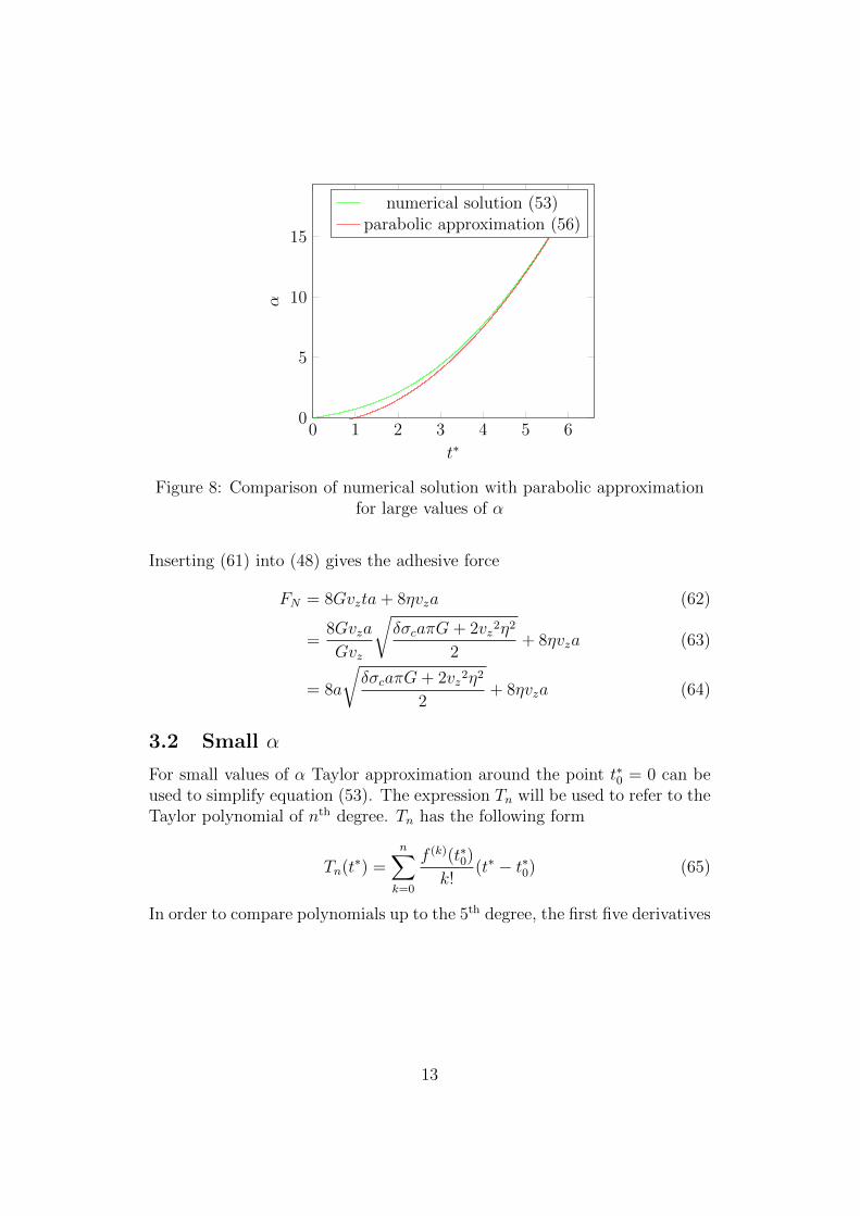
Figure 8 shows both this approximation and the exact solution for largevalues of α.Equation (56) is solved for t in order to get a result for the adhesive force .

α =1

2t∗2 − 1

2(57)

⇔ t∗2 = 2α + 1 (58)

⇔ t∗ =√2α + 1 (59)

⇔ tG

η=

√δσcaπG

2vz2η2+ 1 (60)

⇔ t =1

Gvz

√δσcaπG+ 2vz2η2

2(61)

12

0 1 2 3 4 5 60

5

10

15

t∗

α

numerical solution (53)parabolic approximation (56)

Figure 8: Comparison of numerical solution with parabolic approximationfor large values of α

Inserting (61) into (48) gives the adhesive force

FN = 8Gvzta+ 8ηvza (62)

=8Gvza

Gvz

√δσcaπG+ 2vz2η2

2+ 8ηvza (63)

= 8a

√δσcaπG+ 2vz2η2

2+ 8ηvza (64)

3.2 Small α

For small values of α Taylor approximation around the point t∗0 = 0 can beused to simplify equation (53). The expression Tn will be used to refer to theTaylor polynomial of nth degree. Tn has the following form

Tn(t∗) =

n∑k=0

f (k)(t∗0)

k!(t∗ − t∗0) (65)

In order to compare polynomials up to the 5th degree, the first five derivatives

13

of the right hand side of equation (53), from now on called f(t∗), are needed:

f(t∗) = t∗ (t∗ + 1)− 1

2(t∗ + 1)2

(1− e−t∗

)(66)

f ′(t∗) = t∗ + e−t∗(−1

2t∗2 +

1

2

)(67)

f ′′(t∗) = 1 + e−t∗(1

2t∗2 − t∗ − 1

2

)(68)

f ′′′(t∗) = e−t∗(−1

2t∗2 + 2t∗ − 1

2

)(69)

f (4)(t∗) = e−t∗(1

2t∗2 − 3t∗ +

5

2

)(70)

f (5)(t∗) = e−t∗(−1

2t∗2 + 4t∗ − 11

2

)(71)

Then the Taylor polynomial of 5thdegree around the point t∗ = 0 is

T5(t∗) = f(0) +

f ′(0)

1!t∗ +

f ′′(0)

2!t∗2 +

f ′′′(0)

3!t∗3 +

f (4)(0)

4!t∗4 +

f (5)(0)

5!t∗5

(72)

= 0 +12

1t∗ +

12

2t∗2 −

12

6t∗3 +

52

24t∗4 −

112

120t∗5 (73)

=1

2t∗ +

1

4t∗2 − 1

12t∗3 +

5

48t∗4 − 11

240t∗5 (74)

All Taylor polynomials of lower degree can be determined instantly.

T4(t∗) =

1

2t∗ +

1

4t∗2 − 1

12t∗3 +

5

48t∗4 (75)

T3(t∗) =

1

2t∗ +

1

4t∗2 − 1

12t∗3 (76)

T2(t∗) =

1

2t∗ +

1

4t∗2 (77)

T1(t∗) =

1

2t∗ (78)

Figure 9 shows these Taylor polynomials in comparison with the numericalsolution for α (equation (53)). All polynomials are quite accurate for verysmall values of α, but for larger values T2 is closest to the numerical solution,because the polynomials of higher order diverge earlier and faster.With the Taylor polynomial of second degree as an approximation for theright hand side of equation (53) you get the following equation that can be

14

0 1 2 3 40

2

4

6

8

10

t∗

α

numerical solution (53)T1

T2

T3

T4

T5

Figure 9: Comparison of numerical solution with Taylor polynomials ofvarious degrees

solved for t∗.

α =1

2t∗ +

1

4t∗2 (79)

α =1

2t∗ +

1

4t∗2 (80)

⇔ 0 = t∗2 + 2t∗ − 4α (81)

⇔ t∗1,2 = −1±√1 + 4α (82)

Since t∗ can only have positive values the right solution is

t∗ = −1 +√1 + 4α (83)

Returning to the variables with dimensions one gets

tG

η= −1 +

√1 +

δσcaπG

vz2η2(84)

⇔ t =η

G

(−1 +

√1 +

δσcaπG

vz2η2

)(85)

Inserting this into equation (48) the adhesive force results in

15

FN = 8Gvzta+ 8ηvza (86)

=8Gvzaη

G

(−1 +

√1 +

δσcaπG

vz2η2

)+ 8ηvza (87)

= 8ηvza

(−1 +

√1 +

δσcaπG

vz2η2

)+ 8ηvza (88)

= 8ηvza

√1 +

δσcaπG

vz2η2(89)

3.3 Comparison and Approximation Error

For a comparison of the accuracy of these two results one needs to look againat a graph of the dimensionless variables. In Figure 10 it can be seen that inusing these two approximations one can get sufficiently accurate results fora wide range of system specifications.

0 1 2 3 4 50

2

4

6

8

10

t∗

α

numerical solution (53)approximation for small α (77)approximation for large α (56)

Figure 10: comparison of approximations for large and small α with thenumerical solution

The largest error that can occur will be at the point where the lines intersect,which is at α = 3

2+√3 and t∗ = 1+

√3 = t∗approx. The value of t

∗ numericallydetermined from equation (53) for that same α is approximately t∗ = 2.54519.

16

So the relative error H in t∗ is

H =|t∗approx − t∗|

t∗=

|(1 +√3)− 2.54519|2.54519

= 0.0734 (90)

So the maximum error when using these two approximations is around 7.34%.

4 Limiting Cases of Material Behavior

Closed form solutions can also be obtained for the purely viscous as well asthe purely elastic case. The advantage of these solutions is that they can becompared to results previously published in order to validate the results.

4.1 Elastic Case

If the half-space has no viscous properties, then η approaches zero. In thatcase equation (44) can be simplified to

δ =2Gvz

2t2

σcaπ(91)

therefore

t = ±√

δπaσc

2Gvx2(92)

A negative time t can be ruled out, so

t =

√δπaσc

2Gvx2(93)

Substituting t into equation (48) the adhesive force turns out to be

FN = 8Ga

√δσcaπ

2G=√

32Ga3δσcπ (94)

With 4G = E∗ and δσc = γ12 we get

FN =

√8E∗a3γ12π (95)

which is the same as Kendall’s result for a cylindrical flat punch in adhesivenormal contact with an elastic half space.[3]

17

4.2 Viscous Case

If G approaches zero, the half-space exhibits viscous but not elastic behaviorand equation (48) can directly be simplified to

FN = 8ηvza (96)

Consequently the pull-off force in the solely viscous case does not depend onthe adhesive forces.This might seem surprising, but in fact this relation has already been shownin experiments by Voll and Popov [12][13].

18

5 Conclusion

A mathematical model has been developed for the adhesive contact betweena flat punch and a visco-elastic half-space. While for the general case thepull off force can only be determined numerically, two approximations havebeen identified. Combined they are sufficiently accurate for a wide varietyof systems. Which approximation fits a specific system best is establishedby the value of the constant α, which includes all the specifications of thesystem. For a range of 0 < α < 3

2+√3 the adhesive force will be

FN = 8ηvza

√1 +

δσcaπG

vz2η2

For α > 32+√3 it is

FN = 8a

√δσcaπG+ 2vz2η2

2+ 8ηvza

The approximation error is less than 8%.To verify the validity of the new model two limiting cases of the model havebeen compared to results that had already been published in the past.For further analysis the derivations in this thesis can be used as a guidelineto expand the model in order to include other profiles of contact partners.

19

6 Symbols

a contact radius (m)b Dugdale radius (m)E Young’s modulus (Nm−2)E∗ effective modulus (Nm−2)Fcont contact force (N)FN adhesive force (N)G shear modulus (Nm−2)H relative error of the approximationh z-Position of punch (m)∆k stiffness of foundation (Nm−1)padh adhesive pressure field (Nm−2)qadh linear force density derived from adhesive pressure field (Nm−1)r radial coordinate (m)t time (s)UT total energy of the system (Nm)uz displacement of half-space surface in z-direction (m)vz speed of punch in z-direction (m s−1)x coordinate in reduced system (m)∆x small distance between elements in foundation (m)δ Dugdale distance (m)η viscosity (N sm−2)γ12 surface energy (Nm−1)∆γ damping coefficient of foundation (N sm−1)ν Poisson’s rationσc Dugdale pressure (Nm−2)

20

References

[1] H. Hertz, “Uber die Beruhrung fester elastischer Korper,” Journal furdie Reine und Angewandte Mathematik, vol. 1882, no. 92, pp. 156–171,1882.

[2] K. L. Johnson, K. Kendall, and A. D. Roberts, “Surface Energy and theContact of Elastic Solids,” Proceedings of the Royal Society A: Mathe-matical, Physical and Engineering Sciences, vol. 324, no. 1558, pp. 301–313, 1971.

[3] K. Kendall, “The adhesion and surface energy of elastic solids,” Journalof Physics D: Applied Physics, vol. 4, no. 8, pp. 1186–1195, 1971.

[4] B. V. Derjaguin, V. M. Muller, and Y. P. Toporov, “Effect of contactdeformations on the adhesion of particles,” Journal of Colloid And In-terface Science, vol. 53, no. 2, pp. 314–326, 1975.

[5] D. Maugis, “Adhesion of Spheres: The JKR-DMT Transition Using aDugdale Model,” Journal of colloid and interface science, vol. 150, no. 1,pp. 243 – 269, 1992.

[6] D. Dugdale, “Yielding of steel sheets containing slits,” Journal of theMechanics and Physics of Solids, vol. 8, no. 2, pp. 100–104, 1960.

[7] V. L. Popov and M. Heß, Methode der Dimensionsreduktion in Kontak-tmechanik und Reibung. Springer, 2013.

[8] V. L. Popov and A. V. Dimaki, “Friction in an adhesive tangential con-tact in the Coulomb-Dugdale approximation,” The Journal of Adhesion,pp. 1–15, jul 2016.

[9] V. L. Popov and M. Hess, “Method of Dimensionality Reduction in Con-tact Mechanics and Friction: A Users Handbook.,” Facta Universitatis,vol. 12, no. 1, pp. 1–14, 2014.

[10] K. Kendall, “An Adhesion Paradox,” The Journal of Adhesion, vol. 5,no. 1, pp. 77–79, 1973.

[11] V. L. Popov, “Basic ideas and applications of the method of reduction ofdimensionality in contact mechanics,” Physical Mesomechanics, vol. 15,no. 5-6, pp. 254–263, 2013.

21

[12] L. B. Voll, Verallgemeinerte Reib- und Adhasionsgesetze fur den Kontaktmit Elastomeren : Theorie und Experiment. Doctoral thesis, TechnischeUniversitat Berlin, 2016.

[13] L. B. Voll and V. L. Popov, “Experimental Investigation of the Adhe-sive Contact of an Elastomer,” Physical Mesomechanics, vol. 17, no. 3,pp. 232–235, 2014.

22