University Turbine Systems Research (UTSR) Industrial Fellowship Program

2018

Final Report

Adiabatic Film Cooling Effectiveness: Various Measurement Techniques & Review of Surface Roughness Effects

Prepared For:

Solar Turbines,Inc. 2200 Pacific Highway

P.O. Box 85376 San Diego, CA 92186-­­5376

&

Southwest Research Institute (SwRI) Mechanical Engineering Division

6220 Culebra Road San Antonio, TX 78238-­­5166

Prepared By: Christopher M. Nestor

Graduate Research Assistant Department of Mechanical and Aerospace Engineering

West Virginia University Morgantown, WV 26506-­­6106

Supervised By: Site Mentor: Hongzhou Xu, Senior Consulting Engineer

Michael Fox, Heat Transfer Group Manager Heat Transfer Group

Solar Turbines San Diego, CA 92186-­­5376

Academic Advisor: Dr. Andrew C. Nix

Associate Professor Department of Mechanical and Aerospace Engineering

West Virginia University Morgantown, WV 26506-­­6106

1.0 Introduction Nondimensionally matching gas turbine engine operating conditions allows original

engine manufacturers, OEM’s, and designers the ability to test individual engine components in a scaled, off engine setting before the starting full production. The benefits of component testing include practically every aspect of design from material, structural, and thermal reliabilities, to matching computational fluid dynamics (CFD) predictions. Considering a heat transfer perspective, this type of testing is incredibly important to ensure that hot section components are durable and capable of withstanding the most extreme in-engine operating conditions.

One of the most significant factors characterizing the performance and temperature limits of gas turbine engines is the adiabatic film cooling effectiveness. Film cooling, as the effectiveness name suggests, is a necessity to often meet design criteria while staying within feasibility constraints. This effectiveness details the traits of turbine blade film cooling, and is heavily dependent on a variety of different parameters such as density and blowing hole ratios. Relating the freestream, coolant, and adiabatic blade wall temperatures, this nondimensional value can be found experimentally through several measurement techniques. Measurement methods such as transient liquid crystal (TLC) paint and pressure sensitive paint (PSP) are among the most proven and reliable techniques used in high resolution adiabatic effectiveness investigations. Solar Turbines Inc., among other industrial and academic research facilities, employ these measurement techniques for heat transfer studies. In order to produce valid and meaningful results, such studies also demand careful attention to the experimental setup and wind tunnel conditions.

This report will therein focus on several experimental rig testing parameters, TLC and PSP data analysis, and methodologies employed during a brief, yet robust fellowship rotation. With a supplemental investigation focusing on measurement techniques such as TLC and PSP, primary attention was given to influencing the adiabatic effectiveness performance characteristics in the experimental test section (e.g. wind tunnel design). As previously noted, certain operating conditions such as the general momentum transport properties can have a dramatic effect on the effectiveness value. Therefore, possessing the capabilities to characterize and control mainstream and coolant conditions such as turbulence intensity is important to nondimensionally match engine operating conditions during developmental testing. The use of a constant temperature, hotwire anemometer is one tool implemented to document freestream turbulence facility benchmarks at Solar Turbines. The setup, calibration, and testing procedure is established and documented. The initially thought turbulence intensity for the scaled cascade rig was roughly 11%. Numerical and experimental data aimed to validate this assessment since prior rig turbulence documentation had come into question.

In addition to freestream turbulence characteristics, boundary layer turbulence generated from rough in-coolant hole surfaces is an influential adiabatic film cooling effectiveness parameter garnering new attention. Previously considered unimportant due to the smooth surface finishes of traditional cooling hole manufacturing techniques, new focus is being drawn to the effect of cooling hole surface roughness through novel manufacturing processes such as additive manufacturing. Surface roughness is an area of film cooling research relatively undocumented, and currently has limited published studies. Before petitioning computational fluid dynamic simulations or experimental rig testing, a literature review is conducted to investigate the validity of previous findings and whether additional

experiments need conducted. Please note that for organization in the proceeding sections all references, figures and

table numbers, and any appendices are provided for each specific section to prevent confusion and overlap. The order of the listed projects was completed at varying time intervals and complied for this report. 2.0 Titan 250E Trailing Edge Transient Liquid Crystal Testing

2.1 Introduction & Summary

In order to validate CFD predictions and understand the cooling schemes implemented in the stage 1 turbine blade of a Solar T250 engine, a transient liquid crystal test is commissioned. Another goal of such testing is for validating prior blade tests by comparing heat transfer coefficient results. The testing model is designed, scaled, and printed via stereolithography, SLA, in three main pieces: the core, trailing edge and leading edge as shown in Figure 2.1. Much of the work during this rotation consisted of the TLC paint calibration and ensuring the proper preparations were in place for testing. Unfortunately, testing did not commence until the last week of the authors rotation. Therefore, the pretesting preparations are briefly detailed along with the setup and test parameters.

Figure 2.1 - Scaled T250 Blade

The general methodology of testing was to proceed as follows: liquid crystal paint was applied to the internal leading edge, pressure and suction sides surfaces of the blade models. Thermocouples were installed at specific locations to acquire air temperature change through each passage. Heat transfer tests are conducted by flowing heated air through each blade passage and recording the time dependent paint transition with video cameras. Isothermal tests were performed by flowing ambient air through each passage to characterize the thermocouple response. Pressure tests were conducted by measuring the static pressure of the air during the isothermal testing at specific locations on each blade model. The experimental test setup was to be conducted at Solar Turbines facility in San Diego, California by the approved test engineer.

2.2 Model Prepping & Instrumentation

The test article was prepped for paint, where liquid crystal paint was applied by the lab technician, instrumented with thermocouples calibrated with the new thermocouple calibration process, and then finally assembled. Based on previously established best practices regarding model surface finish quality, the model was inspected by the test requesting engineer prior to beginning the test. The camera setup for the trailing edge model is shown in Figure 2.2.

Figure 2.2 - Camera Setup for the TE Model

The aforementioned thermocouples were calibrated before testing. This calibration included the use of a water bath, and was completed prior to positioning on the blade model. Pressure taps should be flush to the inner surfaces for the static pressure readings. Figure 2.3 below shows the thermocouple locations for the blade trailing edge as a reference.

Figure 2.3 - Model 2 TE SLA shown with TC locations detailed with tag names.

2.3 Liquid Crystal Calibration

In order to calibrate the new TLC paint, a coupon test was commissioned as a reference for paint transition. The liquid crystal paint transition time was recorded in order to ensure that the transition temperature was documented. Based on prior tests and literature, the liquid crystal color transition time should be no more than 22 seconds for the conditions involved. As noted this time comes from literature, and is defined as the maximum allowable time for the transient liquid crystal test without violating the 1-D semi-infinite conduction model assumption.[2] This equation is detailed in Equation 2.1.

𝑡𝑚𝑎𝑥 = 0.1𝜌𝑐𝑡𝑡𝑎𝑟𝑔𝑒𝑡

2

𝑘 (2.1)

In the equation above k represents the thermal conductivity of the clear SLA material, 𝜌 is the material density, c is the specific heat capacity for the material, and 𝑡𝑡𝑎𝑟𝑔𝑒𝑡 is the

thickness of the material. The Figures 2.4 and 2.5 below detail the liquid crystal image analyzer (LCIA) program.

This program analyzes the paint transition color, which correlates to a specific pressure. The calibration is completed the same way as a normal liquid crystal experiment video, with the exception that the calibration process ends at computing the green time. The user then goes to the accompanying excel sheet with thermocouple data from the calibration test, find the start time in the test data, and then can use the max time as indicated from the LCIA to compute green time achieving the calibration transition temperature.

Figure 2.4 - LCIA Calibration Program

Figure 2.5 - Fully Transitioned TLC Paint Coupon

An example of locating the calibration transition temperature is shown in Figure 2.6 below within the Excel spreadsheet. The value should be found around 95 degrees Fahrenheit as suggested by the manufacturer. The figure shows the average thermocouple data giving a transition temperature of 95.4 degrees Fahrenheit. Existing documentation supports similar calibration findings with a previous batch of TLC paint found to have a transition point of 94.5 degrees Fahrenheit.

Figure 2.6 - Calibration Transition Temperature

2.4 Liquid Crystal Image Analyzer (Data Processing)

A new update was released for the LCIA program during testing of this scaled blade. This resulted in several setbacks and a significant amount of time to resolve. Several changes were made to alleviate “glitching” with the program, but introduced new nuances the operator had to become accustomed to. The first is shown in Figure 2.7. When uploading the probe file (file with the thermocouple data for the desired thermocouple point locations), it has been found that the program must say synced in order for the program to accurately proceed.

Figure 2.7 - Probe File Upload

The probe file itself must be manually created by the user from the test cell thermocouple excel sheet. The user will pull out the required thermocouple data sets for the domain window the user wants to run the HTC calculation on and place in a text file. This text file is the probe file that will be uploaded. The format of the text file must look like the following as shown in Figure 2.8 below.

Figure 2.8 - Text File Format

The previous format before the update had a different header line where the first line just had a single number representing the number of rows of temperature data.

The user should be aware of the direction of the flow in the video. This important as the Orientation setting, as shown in Figure 2.9 below, must be appropriately set. If the flow is going from left to right in the window and the heat transfer coefficient, HTC, is desired along the “x-axis” of the screen. The appropriate setting is therefore X Axis in the Orientation drop-down menu. The videos for the scaled testing position the blade where desired HTC is from top to bottom in the viewing window, the appropriate setting is Y Axis in the Orientation drop-down menu.

Figure 2.9 - Orientation Drop Down Menu

2.5 Test Matrix

The testing of the scaled blade began during the week of July 23rd, 2018. Several setbacks in instrumentation, rig setup, and camera setup delayed the testing from the original test data in June/ early July of 2018.

Again, report only briefly highlights the testing procedure, as much of the testing was conducted during this authors rotation out of Solar Turbines. The complete test matrix includes 18 test runs; 9 of which are for the trailing edge model. Tests 1-3 are for the entire model, tests 4-6 detail the suction side of the model, and tests 7-9 detail the pressure side of the model. It is important to note that the tests were required to match mass flow rates, but not necessarily the pressure.

The initial supply air temperature is recommended to be set at 160°F, and can be adjusted in order to ensure that the color transition time occurs within 22 seconds.

Table 2.1 - Test conditions for the TE model

Test Run#

Mass flowrate (lbm/s)

P_inlet (psia)

P_Exit (psia)

PR (P_inlet /

P_exit)

1 0.0383 16.15 14.7 1.0986

2 0.0443 16.65 14.7 1.1327

3 0.0511 17.2 14.7 1.1701

Table 2.1 above lists the test conditions for the first three runs. In the first run, there will be two cameras set up to record the thermal paint transition. During runs 4-6 channels channel 1 and channel 2 should be blocked and the camera should be focused in on the prescribed area as shown in Figure 2.10 below. Table 2.2 below similarly lists the test conditions for the suction side.

Table 2.2 - Test conditions for the SS (Chan3 only)

Test Run#

Mass flowrate (lbm/s)

P_inlet (psia)

P_Exit (psia)

PR (P_inlet /

P_exit)

4 0.0265 17.3 14.7 1.1769

5 0.0306 18.03 14.7 1.2265

6 0.0352 18.92 14.7 1.2871

Figure 2.10 - Configuration for the SS Test (Chan 3 only)

Similar to tests 4-6, test runs 7-9 will be completed, but this time with the pressure side. During runs 7-9 a single camera should be set up to capture the pressure side. Channel 1 and channel 3 should be blocked as shown in Figure 2.11 below. The table list of test conditions for the pressure side can be found in Table 2.3 below as well.

Table 2.3 - Test conditions for the PS (Chan2 Open)

Test Run#

Mass flowrate (lbm/s)

P_inlet (psia)

P_Exit (psia)

PR (P_inlet /

P_exit)

7 0.0258 18.25 14.7 1.2415

8 0.0296 19.2 14.7 1.3061

9 0.0341 20.38 14.7 1.3864

Figure 2.11 - Configuration for the PS Test (Chan 2 Open)

2.6 Results

Unfortunately, the author’s internship rotation ended before all testing data could be completed, leaving little available data to post process as expected. Preliminary data processing with the LCIA software found the following HTC results as shown in Figure 2.12 below.

Figure 2.12 - Preliminary HTC Results for 5X blade

This figure prematurely shows the pressure side of the trailing edge blade heat transfer coefficient, HTC, results after calculating in the LCIA program. These results were not available to export to text file the last day of the author’s internship due to an error with the program’s export feature. This error has been fixed, but time did not allow recalculation of the HTC for this region as it was deemed more important to document the procedure for future reference. While the program ran as completed, qualitative results were not available, and it would be premature to further discuss at this time. This section is included though to leave a point of reference for post processing to resume.

2.7 References

[1] Singh P, Ravi B, Ekkad S. Experimental Investigation of Heat Transfer Augmentation by Different Jet Impingement Hole Shapes Under Maximum Crossflow. ASME. Turbo Expo: Power for Land, Sea, and Air, Volume 5B: Heat Transfer ():V05BT16A018. doi:10.1115/GT2016-57874. 3.0 Pressure Sensitive Pain Calibration

3.1 Introduction & Summary

It is desired to automate the pressure sensitive paint (PSP) data calibration post processing procedure. The prior method for sorting through the calibration data involved

manually copying and pasting the data acquisition system (DAQ) output file(s) into a new Excel workbook with different tabs. Each tab’s data corresponded to the various pressure tests conducted at their respective temperatures. Example data given included 13 pressures each conducted at 9 different temperatures. The code written in MATLAB® Version R2016a mimics this manual procedure replicating the data filtering process.

The following section documents the procedure through which the code was developed, and the instructions for operating the code. The designed algorithm allows a user to select an output file name, save location, and select the working file directory. This program does not modify or change the testing procedure for conducting PSP calibration testing. This program was designed to be robust in allowing for variations in DAQ output file formats; meaning necessary data does not have to be in the same position within the imported files. This design feature is incorporated for the event that there is a formatting change or update with the DAQ software thus leading to a change in the DAQ output file format (i.e. this program’s input file(s)).

3.2 Goals

The goal is to easily display the ratio values of test pressure-to-atmospheric pressure, and the ratio of respective pressure intensity-to-atmospheric pressure intensity. These ratio values are needed to find curve fit user-defined model numeric coefficients. Therein, the described ratio data sets are copied to Curve Expert for analysis. The data is graphed and a user-defined model curve fit is applied. This user-defined model is given as:

𝑦 = 𝑎 + 𝑏 ∗ 𝑥 + 𝑐 ∗ 𝑑 ∗𝑥

(1+𝑑∗𝑥) (3.1)

This equation defines y as the dependent variable, intensity ratio, and x as the independent variable, pressure ratio. Curve Expert calculates the coefficient values (a, b, c, d) required to achieve the user-defined model. According to current knowledge, MATLAB® does possess the capability for internally solving for coefficient values. However current Solar MATLAB® licenses do not possess necessary installed toolboxes for solving nonpolynomial coefficients of a user-defined equation. It is recommended that installing and utilizing the Curve Fit ToolBox within MATLAB® will allow the user to process all data internally, and would eliminate the need to use the Curve Expert software. This therefore, would reduce user-program interaction (i.e. nonessential data handoffs) and further decrease post processing time.

3.3 PSP Description

A brief review of this measurement technique is discussed for the reader’s benefit. This measurement technique is based on the principle of oxygen-quenched photoluminescence. After a light source is exposed to a surface coated in the pressure sensitive paint, the paint emits light with an intensity dependent on the partial pressure of oxygen within the chamber’s surrounding gas. A charge coupled device (CCD) camera is used to record the luminescence reflected off the surface. Since the only light reflected to the camera is from painted surfaces, only the desired surface appears in the images. The intensity of the reflected light is directly correlated to the pressure experienced on the surface of interest. In the interest of understanding this program code, only the intensity measurements, test

section inlet pressures, and operating test section temperatures are required. Therefore, no further detail regarding the operating principle of pressure sensitive paint is necessary, and is thus not provided.

3.4 Packaged Files

The automation program is comprised of 4 script files. One is the entry point displaying a graphical user interface to allow the user to select how to proceed. Relevant information is displayed along with instructions for operating the program. There are two action buttons: one with the option to exit the program and another to proceed to the next window. To prevent unintentional program termination, a popup dialog box issues a warning to the user should the closure action button on the point of entry window be clicked. The main algorithm is called upon after the outputted file name is chosen and the respective location directory chosen.

3.5 Standard MATLAB® Interface/ Implementation

The following is an excerpt from the documented instructional report on how to use the final program. This document allows another user, without knowledge of the PSP post processing procedure, to execute this code. The program requires that MATLAB® be installed and an active license be issued.

1. Open MATLAB® script file called “PSP_Calibration_Begin_v1”. This can be done by either double clicking on the file itself or opening MATLAB® and browsing for the file within MATLAB®’s Open File Window and Browse for the file.

Figure 3.1 – MATLAB® Window

2. Ensure that this specified file has not been moved out of the working directory entitled “Complete PSP Calibration Package”. This directory needs to contain the packaged files listed in the preceding section as shown below.

Figure 3.2 - Working Directory with Required Files

3. Click the Run button located in the Editor Tab of the MATLAB® window.

Figure 3.3 - Editor Tab & Run Button

4. A Graphical User Interface (GUI) will appear with instructions and two buttons for starting or canceling the program.

Figure 3.4 - Start Menu

5. Click Start to begin or Cancel to exit.

6. Clicking Cancel will bring up a dialog alert with a confirmation to close the window as shown in Figure 3.5

Figure 3.513 - Close Window Confirmation

7. Clicking Start will bring up a dialog alert shown in Figure 18 with the instructions to first save the exported Excel file name and file location.

Figure 3.6 - Instruction Prompt

8. Type the file name of the exported Excel file following standard Excel file name conventions. (This is the required output format and cannot be changed unless code modification).

Figure 3.7 - Save File GUI

9. Browse within the GUI to select the file save location. 10. A new GUI will appear asking to select the main folder containing each subfolder of

desired data files to be queued for import. Browse for highest hierarchal folder to establish as the directory.

Figure 3.8 - Select Folder Directory GUI

11. The code will then begin to run and process the files. A popup dialog box will appear notifying the user when the process is complete accompanied with several “beep” sounds. Any errors or warnings will terminate the code in the MATLAB® command window. Refer to code comments to troubleshoot the warnings.

Figure 3.9 - Program Complete

3.6 Advanced Operating Procedure with MATLAB® Application (APP) Interface

MATLAB® R2016a supports application development. This allows users to package script file(s) and commands for simplified distribution. Upon completion of Version 1.0, this program folder was packaged for application use. To use the application (App), it must be installed into the MATLAB® Application Library. The benefit of installing the App, is that after successful one-time install, working directory files are automatically routed within MATLAB® and no concern is needed as to whether the complete file package is saved in the same file location. This truly makes the program, “push to start”.

3.7 Data Handling

Intensity parameters recorded include the mean Intensity, standard deviation of intensity values, maximum intensity, minimum intensity, and sum of intensity values. These values are found within exported .csv files. The file extension for the intensity data must be in the form of Comma Separated Value (.csv) for proper code functionality.

The test section inlet pressure values are found from exported .xlsx files. The file

extension for the test section inlet pressure data must be in the form of Excel Workbook 2003-current (.xlsx) for proper code functionality.

Regardless of data size or required data location within the prompted files in either queued import format (.csv or .xlsx), MATLAB® imports, handles, and exports the data in the desired output format inside the respective temperature tabs.

To account for the possibility of various formatting changes in the data layout, a search algorithm was implemented to find where specific data sets are located within queued import files. These search sections of the main computational algorithm are designated with a “%~~…” section break notation.

3.8 Program Logical Progression

This section describes the logical progression of the written program. This algorithm describes the main driving code (newest_main_code.m) and is the same regardless of Standard Operating Procedure or App starting method. This is a high-level description and is not intended to troubleshoot any encountered runtime errors. Please open the file newest_main_code.m and view the embedded troubleshooting prompts for instructions on errors.

1. Indexes main folder directory 2. Indexes subfolder directories 3. Recognition algorithm to find file name pattern inside selected directory

i. Opens first .csv file within subfolder 1 ii. Copies required data to new excel sheet and logs intensity data within MATLAB®

workspace iii. Closes first .csv file iv. Progresses through each .csv file in the same manner.

4. Opens RETS_###F files and copies test section inlet pressure. i. Searches inside file for location of test section inlet pressure data via search

algorithm 5. Exports TS inlet pressure to newly made output Excel file. 6. Organizes data within spreadsheet to match manual method template. 7. Performs the following calculations:

i. Ambient pressure ratio ii. Intensity difference ratio

iii. Intensity ratio 8. Organizes calculated values according to manual method template. 9. Progresses through each directory subfolder, assigning each subfolder as a tab in the

new excel workbook performing Steps 3 through 8 above until last subfolder processed.

10. Renames first worksheet as Summary tab 11. Terminates program with notification pop-up and several accompanying beeping

sounds.

3.9 Future Work

Future work for this would involve initially developing a standalone program capable of executing the operations via command prompt/terminal as a .exe file. MATLAB® supports

application development of this nature, and can export the operations as a standalone file. With this method of packaging, a MATLAB® license is not required by the user since the code is pre-compiled and executed outside of the MATLAB® workspace. Unfortunately, as with many corporate Information Technology, IT, restrictions, it was not currently deemed a trivial task for the amount of time during the author’s rotation.

3.10 References

[1] “MATLAB Documentation and Support.” MATLAB & Simulink, MathWorks, Inc., www.mathworks.com/help/matlab/index.html.

4.0 Constant Temperature Anemometer

4.1 Summary & Introduction

Turbulence measurements in fluid mechanics detail important flow characteristics significantly tied to the transport of momentum, energy, and mass. This is especially true for a fundamental understanding of turbomachinery design and operation. By incorporating considerations for these three transport properties, design improvements can yield higher performance, durability, and thermal efficiencies. In such applications, the flow regime is inherently turbulent and any design consideration requires knowledge to the extent of turbulence and its impact on the device. Therefore, systems such as a constant temperature anemometer (CTA) are important in defining flow characteristics. These measurements can also be beneficial to validate operating conditions and performance parameters to computational fluid dynamic (CFD) simulations.

Solar Turbines utilizes a state of art Dantec Dynamics CTA hotwire system. This system is setup and established with a variety of hotwire probes, multiple directional mounting probe supports, control unit, and signal processing software. The functionality of this system is robust, and can be configured for a variety of flows and conditions. One of the most useful features of Solar Turbines’ system is the additional probe calibration unit. The calibration unit is “plug and play” with the Dantec StreamWare Pro software and the Streamline Module hardware. This ease of use allows quick and precise probe calibration to alleviate any varying environmental influences such as temperature effects. Due to the importance of these measurements, their facilitation in a research setting, and the potential impact off measurement findings on future testing, calibrations should be conducted prior to each use. Therefore, the calibration process is incorporated in the configuration and setup process. A step by step procedure was detailed for internal Solar use after this author’s departure.

4.2 Background

A broad description of a CTA working principle is discussed for the readers’ benefit. A CTA anemometer functions on the principles of convective heat transfer. A heated sensor immersed in a surrounding fluid directly relates heat transfer from the sensor to the fluid velocity. These sensors consist of fine wires mounted in a variety of configurations depending on the measurement and data the user requires. While this is an intrusive measurement technique, advantages of this type of system include a high temporal resolution, ideal for measuring spectral data such as turbulence. Another advantage is the cost of implementation of CTA systems is comparably less than that of other high-resolution

techniques such as particle image velocimetry (PIV). The following is an expert from the Dantec StreamWare Pro Installation and User Guide

detailing how Solar Turbines’ anemometer operates. “The anemometer works according to the Constant Temperature Anemometer principle where the probe forms part of a Wheatstone bridge. It is kept in balance by the error signal across the bridge diagonal so that the probe resistance, and hence its temperature is kept constant independent of the cooling from the flowing medium. The bridge output voltage is thus always a function of the effective cooling velocity acting on the probe.” [1] Understanding the operating principle of the hotwire system yielded faster troubleshooting response times with a Dantec representative; as well as assurance that the hardware is functioning properly.

4.3 Solar Turbines CTA Hardware

The specifications of Solar’s Streamline Pro system are documented for future Solar use and for general reference. More through detail can be found from the system manufacturer website.

Figure 4.1 - CTA Streamline Pro Hardware

The current system has a 16-channel output National Instruments data acquisition (DAQ) device. The Streamline Pro system is capable of up to 6 channels dedicated to hotwire probe modules. Currently there are only two (2) hotwire probe modules installed. These modules have built in signal conditioners for amplification and signal filtering before analog to digital (A/D) conversion. Each anemometer module supports only one sensor. Therefore, the two-dimensional probe has two BNC connections and each must be plugged into the Streamline Pro device. Since only two anemometer modules are installed, the current capabilities of the system are two (2) single wire probes, or one (1) two-dimensional probe. There is also an input port for a thermistor. This thermistor should always be designated with the Input 1 BNC connection on the front panel of the Streamline Pro hardware.

Table 4.1 - CTA Hardware Specifications Bandwidth 100-250 kHz (max 400 kHz)

Noise with background turbulence of 0.1% of 10 kHz 0.005% Drift 0.5µV per °C

1:20 Bridge Configuration

Table 4.1 above details the specifications of the Streamline Pro hardware unit. It is

important to note that this system is designed with a 1:20 bridge configuration, since advanced users will find the option to change this setting within the StreamWare software.

4.4 Signal conditioner

The StreamWare Pro software allows the computer to automatically apply any filtering, gain, or offset to the signal chain before A/D conversion. The signal conditioner selection should be considered before implementing any experiment setup, but the software’s ease of use allows quick changing of these parameters. Any offset that is applied should cover the input range of the A/D board, but is typically sufficient to cover the output signal of 0-5 Volts. Establishing a gain is useful to improve the resolution of the A/D board. This optimizes the voltage signal to cover a larger range of the A/D board thus enhancing resolution. This would be useful with a lower bit board. High-pass filtering removes lower frequency signals and is needed only when such frequencies need to be removed for spectral analysis. High Pass filtering is made with a first order filter that goes down to 10 Hz. Lastly, low-pass filters will block noise of higher frequencies and prevents aliasing of the signal. The filter is recommended to be as steep as possible. Systems such as Solar Turbines’ CTA normally have a -60dB/decade roll-off, so a low-pass filter can be beneficial case depending. Low pass filtering is implemented to avoid aliasing problems at higher frequencies. The low pass filter is a third order Butterworth filter that goes up to 300 kHz.

4.5 Analog to Digital Conversion Board

There is a way to edit options relating to the CTA signal acquired via the A/D board. The location of these settings will be discussed during the Standard Operating Procedure section of the internally kept Solar documentation. At this time though, the system options and limitations are presented as related to the A/D board. The input ranges can be changed from 0-5 Volts to 0-10 Volts. The default is 0-10 Volts. The sampling rate is defined also in this setting window and needs to be a minimum two times the maximum flow frequency (e.g. the Nyquist Frequency). The sampling rate is reduced by the number of channels in use. Dantec recommends that a 100-kHz board covers most low-to-medium applications. Simultaneous sampling may be required when a correlation between quick sampled multiple channels such in the case of Reynolds shear stress measurement.

4.6 Automatic calibrator & Yaw Accessory

Solar Turbines’ system includes an automatic probe calibrator as previously mentioned. The speed, precision, and accuracy of an experiment is dependent on this step of the setup. Therefore, calibration should occur before any experiment, but to varying degrees of complexity. The calibrator employed here can meet a wide range of free jet velocities accomplished by a variety of nozzles. The specifications for this system are as detailed in Table 4.2.

Table 4.2 - Calibrator Settings

Test Section: Free jet

Velocity range: 0.5 to 60 m/s Yawing Range: -40° to +70°

Nozzle equivalent size: 120 mm2

The calibrator also includes an air filtering unit to remove oil and dust particles from the pressurized flow. This air filter should always be used to supply the calibrator with air to prevent particulate contact with the hotwire probe. The air filter is rated to operate 300 hours at maximum flow.

The calibrator also utilizes a Yaw Accessory for calibrating the two-dimensional probe. This Yaw Accessory should only be used for the two-dimensional probe and not for calibrating the one-dimensional probe. The one-dimensional probe has its own mounting accessory. The benefit of the two dimensional probe is that it allows simultaneous recording of turbulence in two spatial directions. This current system supports three-axial probes as well, but it is not currently configured for such use.

Figure 4.2 - Calibrator & Yawing Accessory

The packaged kit contains an extension for the 120 mm2 nozzle (not shown in Figure 4.2 above). This extension should only be used when a yaw calibration is conducted as it impacts the accuracy of the calibrator. The velocity calibration should be conducted with the probe placed immediately flush at the upper surface of the calibrator nozzle.

Documenting procedures and operating instructions for each probe along with implementation with the calibration system was rather extensive, and this detail is provided for background and reference so that calculating turbulence is put better into context for this document’s reader.

4.10 References

[1] Dantec Dyanamics, “Constant Temperature Anemometry,” DantecDyanamics.com. [Online].

5.0 Turbulence Prediction and Measurement

The main goal of the CTA setup, configuration, and documentation is to validate and ensure that engine operating conditions are nondimensionally matched in the scaled cascade experimental rig. Numerical calculations such as the one proposed in the beginning of this proceeding section aim at predicting turbulence conditions that are later experimentally measured. Both numerical and experimental cases were then compared to the limited

previous wind tunnel data for validation. Description of turbulence and how to predict it are detailed for reference.

5.1 Turbulence Definition

Most flows occurring in nature are inherently turbulent; such are the conditions experienced in a gas turbine compressor or turbine. Specific knowledge is required to properly account for and predict control volume outlet conditions in these devices. To completely define turbulence is rather difficult though in one brief statement. According to Mathieu and Scott, there are 11 defining attributes that most thoroughly and completely conceptualize turbulent flows [1].

1. Turbulence is/appears to be stochastic or chaotic in both the time and space domains. Though there is structure to eddies in the flow, the Navier-Stokes equations which govern all incompressible Newtonian flow are deterministic; there is a sensitive dependence on initial conditions yielding a clear average behavior but irreproducible in detail.

2. Occurs always in three-dimensional space. Without such consideration, dissipation scales and stretching of vortices is not considered.

3. Vorticular development of a large-scale range of fluctuating vorticity in random generation.

4. Dissipative with energy when at the smallest eddy scales (Kolmogorov length scale (k) in the form of heat through a cascading effect.

5. Obeys the Navier-Stokes Laws, however, is unlikely to be comprehensively predicted by a solution.

6. Non-linear phenomena due to the convective acceleration term Navier Stokes equations and leading to nonlinear Reynolds Stress development.

7. High Reynolds number phenomena resulting from instability at higher Reynolds values.

8. Continuum phenomena where the smallest eddy scale is determined at the Kolmogorov scale which is greater than the mean free path. The Kolmogorov scales tend toward being homogenous, isotropic, and universal as Reynolds number is increased.

9. Large ranges of length and time scales for eddies that become independent of Reynolds number for large Reynolds numbers. At these high Reynolds numbers, large eddies become almost inviscid.

10. Behavior is often intermittent. 11. When concerning mass transfer, turbulence is a diffusive phenomenon. Only using these characteristics can a turbulent flow be properly defined. When

measuring turbulence in nature or within a laboratory setting, the main quantifiable terms detailing these eleven characteristics are the turbulence intensity and the turbulent length scale. These two parameters are most commonly found after a Reynolds decomposition of the velocity signal, and an autocorrelation respectively.

5.2 Calculating Turbulence Intensity & Length Scale With A Grid

One of the most commonly used methods of controlling freestream turbulence parameters is using a flow grid system. This grid system can be either active or passive. The

passive system is more cost effective than the former, and is simple to implement. Assuming flow conditioners are used in the upstream sections of the grid location, the flow arrives at the turbulence grids in a laminar state. Taking advantage of the turbulence vortex shedding principle, the size and scope of downstream turbulence can be directly modified depending on grid bars shape and size. Two lattice style grids trip the flow to the turbulent state in conventional configurations. Extensive empirical data collected by Baines and Peterson have found correlations between grid size and shape to turbulence intensity and integral length scales downstream of a turbulence grid [2]. The following is a process of finding the intensity and vortex integral length scale sizes. It is important to note that the length scale discussed is the largest size (integral length scale) and does not predict Kolmogorov or Taylor-micro scales. The numerical approximation is detailed first followed by the experimental process for finding the turbulence intensity and length scale.

The Turbulence Intensity (Tu) and length scale (𝛬𝑥) decay are functions of the normalized stream wise distance, x. These parameters can relatively be well approximated via:

𝑇𝑢 = 𝑐 (𝑥

𝑏)

𝑛 (5.1)

𝛬𝑥 = 𝐼𝑏 (𝑥

𝑏)

𝑚 (5.2)

I is a constant equal to 0.20, b is the bar characteristic length (i.e. diameter or cross-sectional width), c is given in Table 5.1 for the type of bar and setup (1.13 for parallel square and square mesh grids), m is a constant given as 0.54, and n is a constant given as -5/7. The bar diameter is the appropriate dimension to use and is confirmed via experimental data. [3] The constant c is a function of grid geometry reflecting the drag force experienced by individual elements of the grid. It is presented in literature that it is not necessary to estimate any grid pressure losses to find the downstream turbulence energy. [3] For fully isotropic flow, all three spatial coordinates are ideally equal. Grid turbulence has been generally found to not be truly isotropic, but relations have been found to approximate each spatial coordinate. Reviewed here is the stream-wise direction. Table 5.1 below details the coefficient values for all various standard grid geometries. Experimental data has shown that parallel arrays of square bars and square-mesh arrays of square bars agree well with each other, and for the purposes of Solar Turbine’s scaled cascade rig, no distinction between the two is needed. A working Excel calculator was developed to calculate the predicted turbulence intensity and length scale with inputs for stream-wise distances and bar diameter (Excel program not attached). The program also allows the user to select the type of grid shape, accounting for any bar cross sectional area configuration.

Table 5.1 - Grid Values [4]

(SMR= Screen Mesh Round, SMS= Screen Mesh Square, PR= Parallel Round, PS=Parallel Square)

5.3 Processing Measured Turbulence

There are two methods of experimental turbulent-flow analysis: one using a statistical theory of turbulent correlation functions, and the other a semi-empirical turbulent modeling of mean quantities [5]. The first method utilizes the frequency, oscillations, and other statistical interactions with each other. The second employs more engineering relevance with mean velocity, temperatures, wall friction, heat transfer, shear thicknesses and root-mean-square fluctuations. The method detailed here utilizes mean values and various statistical relations.

When post processing turbulence data, the flow must be expressed in terms of mean values, 𝑈, and superimposed turbulence fluctuations, 𝑢′ as shown in Figure 5.1 below. The equation for a measured value of velocity at a given sample time, ��, can be expressed as a summation of the mean velocity, 𝑈, and the fluctuating velocity component, 𝑢′ as follows in Equation 5.3 [6]:

�� = 𝑈 + 𝑢′ (5.3)

Figure 5.1 – Time-averaged and fluctuating velocity of turbulent flow [7]

Figure 5.1 details a raw velocity signal with a visual depiction of the fluctuation and time-averaged values. The time mean value for velocity, 𝑈, like the equation previously discussed is represented by the expression:

𝑈 =1

𝑇∫ 𝑈(𝑥, 𝑦, 𝑧, 𝑡)𝑑𝑡

𝑡𝑜+𝑇

𝑡0 (5.4)

with the time interval, T, representing a considerably longer time than that of the longest fluctuation period, but shorter than an average velocity unsteadiness. Assuming an evenly distributed range of fluctuations on either side of the average, and realizing that the square value of the fluctuation mean cannot be zero as expressed in Figure 5.2 below, the level of turbulence or turbulence intensity can be found.

Figure 5.2 - Average of Fluctuations and Average Square of Fluctuations Imposed on Signal [7]

The turbulence intensity varies from one flow situation to another, and can be large in a strong headwind or smaller in a lighter yet still turbulent breeze. This value quantifies such scenarios mathematically as the root mean square of the average of the fluctuation squared over the average velocity:

𝑇𝑢 =√(𝑈′)2 2

𝑈=

𝑈𝑟𝑚𝑠′

𝑈 (5.5)

This equation can reflect both the time and frequency domains. The 𝑈𝑟𝑚𝑠′ value in the

Streamline Pro software is represented as the standard deviation, Std. Dev., value given in the Basic Statistics analysis. This parameter is also known as the 2nd order central moment in statistical analysis. A larger turbulence intensity value is contributed to larger fluctuations in velocity. This value is set according to a passive bar grid design placed upstream of the test section as previously described.

As noted, the value of 𝑈𝑟𝑚𝑠′ , is the root mean square (RMS) for the fluctuating velocity

signal can also be determined in the frequency domain using the power spectral density (PSD) for the fluctuating velocity component. The PSD yields an exemplification of the energy at each frequency of turbulent fluctuation, also known as the eddy scale. Integrating this spectrum would yield the fluctuating energy. Utilizing a fast Fourier transform (FFT), the fluctuating velocity component of the signal is decomposed, and the RMS value can be found thus providing the turbulence intensity. This process can also be achieved via the Streamline Pro software by selecting the Power Spectral Density analysis in the same menu as the Basic Statistics. Detail of this method though, is not extensively detailed in this report, and the time averaging procedure is instead used.

The turbulent eddy time-scale is an additional term used to characterize turbulence. This parameter is found based on the peak to peak distance of the measured maximum turbulence intensity using an autocorrelation technique. The autocorrelation (R11) of the fluctuating velocity component can be used to calculate the integral time scale (T) by integrating under the curve to the first zero crossing as the lag time (τ) goes to zero. The RMS value of the velocity signal squared yields the unnormalized value of the autocorrelation.

The integral turbulence length scale is found by using the integral time scale, 𝑇𝑚, found from time integral of the autocorrelation curve of the fluctuating part of the velocity, 𝑅11 as shown in Equation 5.6 below.

𝑅11(𝜏) =𝑢(𝑡)∙𝑢(𝑡+𝜏)

𝑢′2

=

1

𝑁(

∑ 𝑢𝑖∙𝑢𝑖+𝑗 𝑁1

𝑢′2 ) (5.6)

where 𝜏 is the total autocorrelation lag time equal to the product of the number of total time steps, j, with the time step, ∆𝜏, going toward zero.

𝑇𝑚 = ∫ 𝑅11∞

0(𝜏)𝑑𝜏 = ∑ 𝑅11∆𝜏

𝑁0𝑖 (5.7)

Expressed in integral form first, the expression for the time integral scale can be approximated in summation notation until the first zero crossing, 𝑁0, via the right-hand side of the above Equation 5.7. Summation is only to the first zero crossing due to noise that exists in the auto-correlation. Using this value, the integral length scale, Λ𝑥, representative of the largest eddies in the turbulent flow field, is found from the product of the integral time scale

and the mean velocity as shown in Equation 5.8:

Λ𝑥 = 𝑈 ∗ 𝑇𝑚 (5.8)

Equation 5.8 is representative of Taylor’s hypothesis of frozen turbulence, expressing Λ𝑥 to represent the distance between the largest subsequent turbulence eddies corresponding to recorded “hits” of the data acquisition system as vortices are generated.

Other important statistical parameters that yield important information about turbulence are the 3rd central moment called Skewness and the 4th central moment called Kurtosis. Skewness details a dataset’s symmetry in a numerical distribution. Symmetrical datasets will have a skewness equal to zero. Kurtosis is a statistical measurement of the “flatness” of the turbulence data set. A time series data set with measurements clustered around the mean value will have a low kurtosis value. Conversely, a data series dominated with intermittent extreme peaks will have a higher kurtosis. Datasets with varying degrees of kurtosis and skewness are shown in Figure 5.3 below for reference. These parameters offer supplemental information about the turbulent flow field, and is only necessary when it is desired to “fully and completely” statistically describe the flow.

Figure 5.3 – Skewness and Kurtosis example datasets [8]

5.4 Experimental Results

5.4.1 Calibration

Utilizing the author’s documented procedure for completing a test with the Dantec hotwire, a calibration was conducted. The results of the calibration are as shown in Table 5.2 below. The calibration settings were set with a range of 5 to 35 m/s in equal increments for testing. The sampling rate was set at 1000Hz and the automatic calibrator dwelled at each sampling point for approximately 1 second. This setting was predetermined as default by the calibrator unit. The calibration settings were always set to ≤ 0.25% reading error of the pressure transducers in the automatic calibrator. The calibration was conducted outside of the cascade wind tunnel. Using a thermistor, temperature corrections would be applied for the obvious change in temperature that would occur in the scaled cascade wind tunnel test section.

Table 5.2 – Calibration Results U U1calc

9.988 9.980 11.669 11.677 13.608 13.626 16.528 16.520 18.476 18.456 21.580 21.577 25.151 25.144 29.385 29.418 34.257 34.252 39.967 39.958

The resulting velocities, after signal processing, and applied desired calibration

corrections are found to be extremely close to the target value. This calibration was conducted for a single wire probe only; although the procedure for the two dimensional probe was documented for Solar Turbines reference. In the case of the two dimensional probes, directional calibration is also required to compensate for varying oncoming leading angles of attack; hence the need for the yaw manipulator and directional calibration as previously discussed. Shown in Figure 5.4 is the resulting calibration curve from one, one-dimensional calibration trial.

Figure 5.4 - Calibration Curve

Upon searching through Solar Turbines archived documents, it was found that when the

wind tunnel of interest was created, various turbulence grids and their respective turbulence intensities were benchmarked. This data had fallen out of notice, and current conditions were known, but not certain. While the length scale is also an important factor for turbulence calculations as previously noted, for ease of comparison, only the turbulence intensity is deemed necessary for data validation in this situation. Later testing should compare length scale benchmarks. It was found that the particular grid installed should expect a freestream turbulence intensity of 5.60%. Figure 5.5 shows an example of the passive grid documented and tested.

Figure 5.5 - Passive Grid System

Utilizing the numerical approach given by Equations 5.1 & 5.2, the turbulence intensity was calculated and expected to be 5.55%. This value was calculated at the direct downstream length from the grid as the kiln probe (i.e. right before the leading edge of the scaled turbine blades in the tunnel test section). This location is not disclosed for this report. After performing the required calibration, setup procedure, and experimental runs, the experimental turbulence intensities were found via the StreamLine Pro integrated software. The hotwire was positioned at the leading edge of the scaled turbine blade in the tunnel test section. Since turbulence decays with streamwise length from the grid, this location would ensure that the turbulence experienced is similar to that found leading onto the scaled blades. Tests were conducted at the sample sampling rate as calibration runs, and dwelled live for approximately 15 seconds. This data was then automatically post processed, corrected, and time averaged for the turbulence intensity and length scales. Time to freestream steady state was determined by the kiln probe signaling a recording as close to a semi-steady temperature as possible within the tunnel. The resulting average length scale experimentally found after 5 trials was 5.80%. The experimental value of 5.80% is assumed higher than the numerical and prior benchmark for two main reasons. This value is an averaged turbulence intensity with data mostly likely recorded when temperatures were still stabilizing and the thermistor hadn’t sufficiently reached freestream conditions. Additionally, due to mounting configuration limitations within the cascade tunnel, the resultant hotwire location was placed further upstream than originally anticipated. This streamwise relocation was minor, but could have had a significant influence on the turbulence intensity. Even though this value is slightly higher than that of the numerical prediction and the previous benchmarked data, it is not outside of an acceptable error band for characterizing general turbulence; especially in this case where a general range was desired. It should be noted that most of the data agreed closer to the 5.65%-5.70% turbulence intensity range with a few data samples closer to the higher values of 5.85% and 5.90% turbulence intensity. In this situation more details regarding the turbulence could be found from calculating the skewness and flatness of the data sets. These higher values were noted to correlate where temperatures were most likely still rising in the free stream tunnel conditions.

Final conclusions yield that the original perception of the free stream turbulence intensity near approximately 11% in the scaled cascade tunnel test section inlet is incorrect. While further testing is recommended with higher sampling rates and more data samples to increase data resolution, all predictions and results conclude that the actual turbulence intensity is closer to that of approximately 5.7%-6.0%. While length scales were not deemed important for this generalized characterization and proof of concept, the enhanced resolution and sampling size will refine the length scale values. Then with both parameters found within a tolerable error range, can the exact tunnel turbulence can be fully characterized. Additionally, other turbulence grids must be fabricated according to the analytical prediction equations previously given (Equations 5.1 & 5.2) and validated in the tunnel should a higher turbulence be desired in the scaled cascade rig.

5.5 References

[1] J. Mathieu and J. Scott, An Introduction To Turbulent Flow. Cambridge University Press, 2000.

[2] W. D. Baines and E. G. Peterson, “An Investigation of Flow Through Screens,” Am. Soc. Mech. Eng., pp. 467–480, 1951.

[3] P.E. Roach,The generation of nearly isotropic turbulence by means of grids, International Journal of Heat and Fluid Flow, Volume 8, Issue 2, 1987, Pages 82-92, ISSN 0142-727X.

[4] Roach, P.E..(1987). The Generation of Nearly Isotropic Turbulence by Means of Grids. International Journal of Heat and Fluid Flow. 8. 82-92. 10.1016/0142-727X(87)90001-4.

[5] F. M. White, Viscous Fluid Flow. McGraw-Hill Higher Education, 2006.

[6] J. Sauer, “The SUDI Turbulence Generator – A Method to Generate High Freestream Turbulence Levels and a Range of Length Scales,” University of Wisconsin/University of Karlsruhe, Germany, 1996.

[7] B. R. Munson, T. H. (Theodore H. Okiishi, W. W. Huebsch, and A. P. Rothmayer, Fundamentals Of Fluid Mechanics. John Wiley & Sons, Inc, 2013.

[8] Tomos W. David, David P. Marshall, Laure Zanna, “The statistical nature of turbulent barotropic ocean jets”, Ocean Modelling, Volume 113, 2017, Pages 34-49, ISSN 1463-5003 6.0 In-hole Surface Roughness Literature Review

6.1 Introduction

The last project during this rotation was reviewing what research existed regarding in-hole surface roughness effects on heat transfer. This information was collected and presented to the heat transfer group for discussion, and how it applies to novel additive manufacturing.

The durability of gas turbine engines is directly related to the engine components’ operating temperatures. Operating at higher temperatures increases the thermal efficiency of the engine, but occurs at the expense of component life and the potential increase of maintenance costs. In the combustor and the turbine inlet stages sections, turbine airfoils and end walls utilize film cooling to reduce the component surface temperatures. Film cooling in its idealized configuration allows coolant ejected through discrete cooling holes

along the blade surface to remain attached to the airfoil surface decreasing the local fluid temperature. Additionally, film cooling makes use of convective cooling, transporting hotter local gases away from the airfoil surface. One of the main calculated parameters of film cooling is the adiabatic film cooling effectiveness. Factors affecting film cooling performance and the adiabatic film cooling effectiveness are the coolant and mainstream conditions, hole geometry and configuration, and the blade airfoil geometry.

Much literature exists on the performance effects of hole geometries and varying coolant/mainstream flow properties. Not significantly published in literature is the influence of coolant hole interior surface roughness on the adiabatic effectiveness. Since prior manufacturing techniques consistently produced “smooth” cooling holes, not much concern toward surface roughness was needed. Now with the adaptation of additive manufacturing and alternative cooling hole development in industry production engine components, the interior surface roughness effects on the adiabatic effectiveness is uncertain, and is drawing new research attention. One of the main and only prominent investigations detailing surface roughness effects was conducted by Schroeder and Thole at Pennsylvania State University. Schroeder and Thole clearly state early in the article that the work presented is the foundation of this area of research [1]. The publication date of the article was March 2017, and is the most recent publication found as of June 8th 2018 in this area of film cooling. There are subsequently published articles focusing on the surface roughness of additively manufactured cooling holes, an area of growing interest to gas turbine manufactures. This review presents a concise summary focusing primarily on the Schroeder and Thole publication with additional comparison to freestream flat plate roughness investigations.

6.2 Previous Research

As noted, this is a novel area of film cooling research with minimal existing open literature. Of the previous work completed, much of the foundation for in-hole roughness stems from a method called “rifling” inside cooling hole geometries. Rifling is essentially grooves cut into the walls of the cooling hole, and it has the potential to increase the effectiveness by “guiding” coolant flow out of the hole. Thruman et al. found an increase in laterally averaged effectiveness when using rifled holes axially oriented of a groove depth of two-tenths times diameter (0.2D) [2]. Since advanced and more rapid manufacturing techniques leave a more irregular surface roughness, the described effect of rifling doesn’t directly correlate. Roughness sizes typical to industrial and aero engines is on the scale of 0.002D<Centerline Average Roughness Height<0.2D.

Much of the existing surface roughness literature pertaining to turbine blade cooling is for rough exterior surface flat plate cooling. Exterior surface roughness effects are well researched and were initiated in the latter part of the twentieth century. Such investigations focus on environmental deposition on turbine blades, and the subsequent heat transfer effects. One study conducted at the University of Texas at Austin by Schmidt et al. sought to understand how surface roughness representative of an in-service turbine blade affects the adiabatic film cooling effectiveness and heat transfer coefficient of a round hole. Schmidt et al. found that for a rough exterior flat plate (i.e. the turbine blade surface) increasing the surface roughness slightly degraded the film cooling effectiveness near the holes along the centerline. This degradation continued to increase up to as much as 30% further downstream from the cooling holes’ location [3]. This study also found that the decrease in effectiveness was the highest at low momentum blowing ratios in opposition to high

momentum blowing ratios. This is because at higher blowing hole ratios the cooling jet experiences “lift off” from the surface. The higher momentum blowing ratios tend to dissipate the injected flow and prevent it from penetrating far into the mainstream. These higher blowing ratios therefore saw improved effectiveness, but at a cost of overall lower film cooling performance. The roughness values caused a greater lateral spreading of the coolant further downstream of the holes resulting in a laterally averaged effectiveness practically similar to a smooth surface [3]. There was not a significant decreased in heat transfer rates, but as mentioned a significant loss in overall film cooling performance occurs due to increased heat transfer rates from the surrounding gases and the surface [3].

The study conducted by Schmidt et al. validated a previous similar study conducted by Goldstein et al. at the University of Minnesota. Schmidt et al. sought to understand the effects of surface roughness typically experienced in a relatively dirty environment. This study used a single and dual row of holes for testing and comparison. The single row of holes experienced an increase in effectiveness at larger blowing ratios, but only marginal increases with two rows at similar conditions. At low blowing rates, there was a noticeable decrease in the adiabatic effectiveness ranging from 10% - 20% for rough surface over that compared to a smooth surface under similar conditions. At higher blowing rates, the jets tend to lift-off from the surface, the film cooling performance is improved significantly, by as much as 40% - 50% percent, under the same conditions as smooth holes [4]. Similar to the other study, this type of effectiveness improvement has caveats (i.e. negatively affecting the overall performance). Again, only minor improvements occurred when comparing single row of holes to dual rows. Goldstein concludes that with rougher surfaces the magnitude of the heat transfer coefficient is expected to be larger than smooth surfaces regardless of the coolant presence.

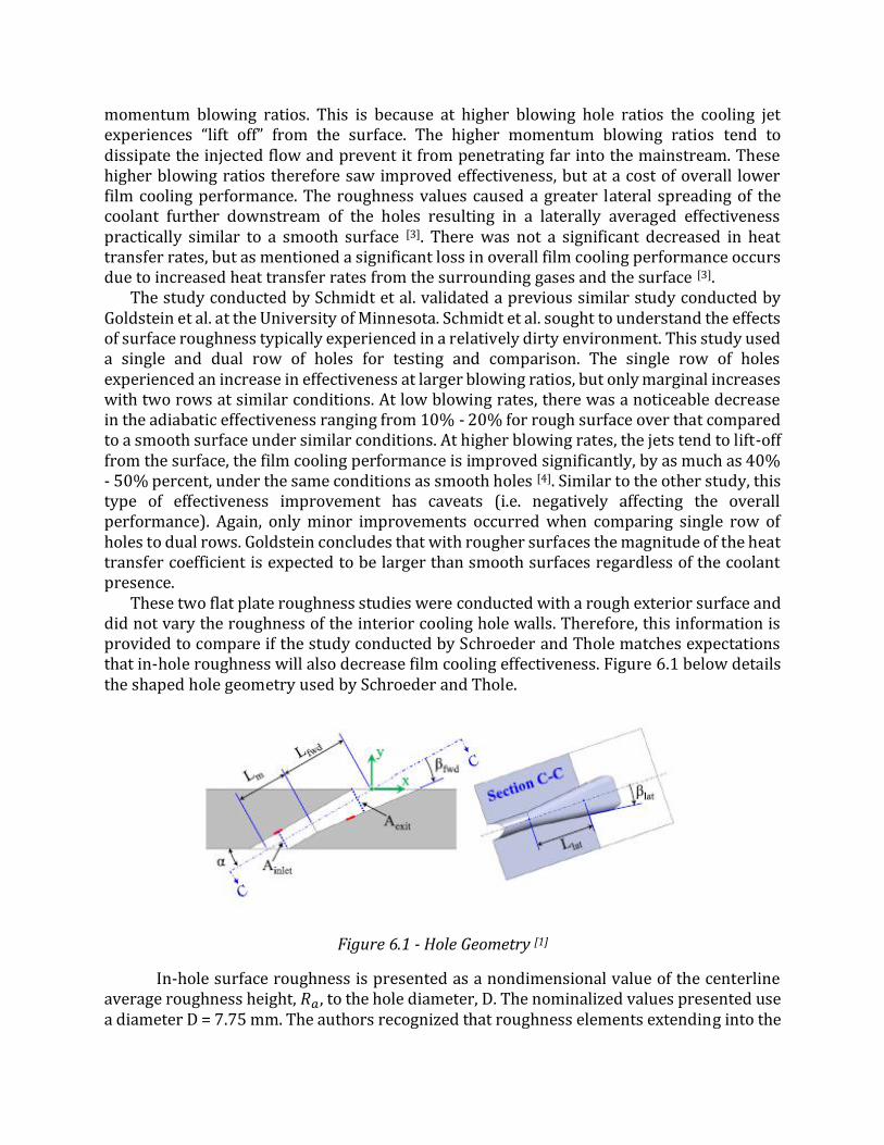
These two flat plate roughness studies were conducted with a rough exterior surface and did not vary the roughness of the interior cooling hole walls. Therefore, this information is provided to compare if the study conducted by Schroeder and Thole matches expectations that in-hole roughness will also decrease film cooling effectiveness. Figure 6.1 below details the shaped hole geometry used by Schroeder and Thole.

Figure 6.1 - Hole Geometry [1]

In-hole surface roughness is presented as a nondimensional value of the centerline average roughness height, 𝑅𝑎, to the hole diameter, D. The nominalized values presented use a diameter D = 7.75 mm. The authors recognized that roughness elements extending into the

hole from the hole walls would reduce the cross-sectional area. To mitigate this area change, small offsets were used in the CNC programming intended to ensure an equal cross-sectional area between specimens. Later measurements detail that hole entrance and breakout dimensions were within 5% of design intent; where the rough diffusor hole was up to 9% larger than nominal. Surface roughness characterization was completed after testing by cutting the specimens apart and measuring surface heights with an optical profilometer. The range of surface roughness values are detailed in Table 6.1 below:

Table 6.1 - Roughness Definitions [1]

Specimen name Range of 𝑅𝑎/𝐷 Smooth hole 0.003-0.004 Slightly rough hole 0.006-0.009 Rough hole 0.017-0.020 Rough diffuser hole 0.016-0.021

As this is one of the first investigations of this nature, the definition of the surface roughness is established as such. It is expected that future investigations will use similar nomenclature. Further inquiries regarding the experimental facility and flow characteristics such as boundary layer dimensions should be directed toward the article as referenced.

6.3 Data

Considering brevity for this review, the following section summaries and condenses the results of Schroeder and Thole as previously introduced. Shown in Figures 6.2 and 6.3 are the decreases in laterally averaged effectiveness from the smooth hole to the progressively rough in-hole surface.

Figure 6.2 - Laterally averaged effectiveness at M=1.5 [1]

Figure 6.3 - Laterally averaged effectiveness at M=3 [1]

Figure 6.4 depicts the contour map of adiabatic effectiveness for the various roughness

scenarios at the blowing ratios tested of 1.5 and 3. The adiabatic effectiveness was found via

infrared thermography. It is evident that for the rougher the hole, the resultant effectiveness value is comparably less than the smoother holes. The wide spread of coolant over the surface is more significant in the lower blowing ratio than in the higher blowing ratio scenario. This wide spread of coolant is also present in the exterior surface roughness studies previously introduced.

Figure 6.4 - Contours of Contours of adiabatic effectiveness for (a) smooth holes, M=1.5; (b) slightly rough holes, M=1.5; (c) rough holes, M=1.5; (d) rough diffuser holes, M=1.5 and (e) smooth holes, M=3.0; (f) slightly rough holes, M=3.0; (g) rough holes, M=3.0; and (h) rough

diffuser holes, M=3.0. Center hole in the row of five is shown. [1]

A useful comparison between the effect of various values for surface roughness is shown in Figures 6.5 and 6.6. Figure 6.5 shows the percent change in area averaged effectiveness between the different in-hole roughness setups to the smooth hole. Similarly, Figure 6 shows the percent change of turbulence intensities for smooth holes to rough diffuser holes at blowing ratios of 1.5 and 3. The significance of the data presented in Figure 6.6 is that freestream turbulence does not drastically change the effects of in-hole surface roughness. The general trend is the same for both free stream turbulence intensity regimes of 0.5% and 13.2%. All scenarios were conducted at a lower freestream turbulence intensity of 0.5% and a higher turbulence intensity of 13.2% via a turbulence grid plate insert. This is important to note since the investigation also sought to understand the influence of freestream turbulence coupled with surface roughness effects. Regardless of freestream turbulence, a resulting decrease in adiabatic averaged effectiveness occurred.

Figure 6.5 - Percent change in area-averaged effectiveness from smooth hole for different

roughness configurations [1]

Figure 6.6 - Percent change in area-averaged effectiveness for high and low turbulence

intensities from smooth hole and rough diffusor holes [1]

Figure 6.7 details the thermal field contours for comparison of a smooth and rough hole. Achieved via a thermocouple rake and the IR camera, the figure illustrates the increased dispersion of the nondimensional fluid temperature, 𝜃, for the rough hole scenario. This data is only given for the higher blowing ratio, documenting the case where coolant flow experienced jet lift extending the coolant further into the freestream flow. Coolant dispersion into the freestream for the rough hole increases the height of the coolant flow boundary layer to a y/D value of 4. Further detail of the “lift off” phenomenon is described in Figure 6.8.

Figure 6.7 – Thermal Field contours at M=3 in z/D=0 centerline plane for smooth hole (top) and rough hole (bottom) [1]

Figure 6.9 shows that the surface roughness contributes directly to an increased lift off angle from the blade surface. The velocity vectors detail that detachment of the coolant stream from the plate surface occurs further upstream for the smooth hole. The rough hole sees almost immediate surface detachment enhancing mixing and increasing heat transfer.

Figure 6.8 – Mean velocity vectors and contours of mean stream wise velocity at DR=1.5, M=3, for smooth hole (top) and rough hole (bottom) [1]

Figure 14 – Contours of turbulence intensity in the centerline plane at DR=1.5, M=3, for the smooth hole (top) and rough hole (bottom) [1]

The turbulence intensity of the coolant jet is higher in the rough hole than the smoother hole. This is visually depicted with a contour map of turbulence intensities found and illustrated in Figure 6.9. As expected, introducing the surface roughness ensures that the flow exiting the coolant hole is further mixed and is fully turbulent as opposed to a smooth in-hole surface where a transitional regime is more likely. In addition to the higher turbulence intensity effects, the interior hole roughness also increased the in-hole boundary layer thickness. This boundary layer thickness increase, further escalated the mean core coolant velocity. Increasing this core velocity, would in turn be a reason for the higher lift off angle and contribute to higher exit turbulence intensity. Figure 6.10 below illustrates that

for every increased surface roughness situation, at any blowing hole ratio, the penetration angle of the coolant into the freestream is higher. Increasing the penetration angle is not normally desired as for the same reasons found in flat plate surface roughness investigations (i.e. the overall film cooling performance is decreased).

Figure 6.10 – Penetration angle of averaged time velocities along y/D=0.4 in the centerline plane for smooth holes and rough holes M=1.0-3.0 [1]

6.4 Application to Additive Manufacturing (AM)

Additional work has been completed by Stimpson et al. at Pennsylvania State University on this type of roughness investigation with additively manufactured blades and cooling holes. The natural progression of the industry is toward applying additive manufacturing with 3D printing to gas turbine engine components. Careful attention is given here to discern the difference between additive manufacturing with 3D printing and the larger broad term of just additive manufacturing. The term additive manufacturing alone could in definition just refer to merging two or more parts with processes such as brazing. Currently, one of the main limiting factors inhibiting such widespread adaptation of additive manufacturing with 3D printing is the resulting material surface finish and gradual deformation during printing. This study was aimed at examining the effects of roughness and building tolerances on the film cooling holes printed via laser powder bed fusion (L-PBF). High temperature nickel alloy coupons were made with various size scaled film holes and tested in a rig simulating engine relevant conditions. Heat transfer experiments showed that the roughness of the additive manufacturing process significantly influenced the overall effectiveness through several mechanisms: film cooling, in-hole convection, and internal convection. The significant blockage in the smaller holes minimized mass flow of coolant through the hole for a given pressure ratio which limited the contribution of film cooling to the overall effectiveness [5]. The investigation compared the additive manufactured holes to those made traditionally via electrical discharge machining (EDM). It was found that the relatively smooth EDM holes had a higher overall effectiveness than the AM holes due to increased film effectiveness. Further

development on this study detail angled and vertical printing of cooling holes and compared results. Other influential cooling hole conditions associated with AM cooling holes is presented such as build angle and direction. It was found that a vertical build direction produces relatively smoother holes than horizontally building cooling holes and there is a difference in their impact on effectiveness values. Extensive regarding build angle and directional effects on adiabatic effectiveness are not included within this review since only the general impact of surface roughness on the adiabatic cooling effectiveness is in current inquiry. Again, this description is provided to supplement findings of surface roughness studies, and details the progression heading of current and future research investigations.

6.5 Conclusions

The study conducted by Schroeder and Thole used shaped holes with different degrees of surface roughness inside the interior walls of cooling holes. Conclusions state that adiabatic effectiveness severely decreased with increased roughness sizes. The most extreme case was a 60% area-averaged effectiveness decrease due to the largest tested in-hole roughness size at the highest blowing hole ratio.

The influence of the in-hole roughness is a function of the blowing ratio. As previous studies found adiabatic effectiveness decreases in traditional smooth holes at higher blowing ratio. This holds true for varying in-hole surface roughness sizes, with larger roughness levels further determinantal to the effectiveness value.

Increasing the blowing ratio generally promotes thinner sub-viscous layer heights in cooling hole geometries. An important ratio to consider is the roughness size to the boundary layer thickness. Schroeder and Thole detailed that this ratio was significant in determining the extend of adverse effects of the surface roughness on the interior wall boundary layer. Surface protrusion elements characterizing the extend of surface roughness were more influential when extending beyond the sub-viscous layer of the turbulent boundary layer within the hole. Larger roughness sizes, increased the probability of the roughness element heights extending above the sub-viscous layer height. An increased interior hole wall boundary layer resulted in faster core-jet flow with correspondingly higher pentation angles leading to faster coolant separation outside the hole. This faster core velocity also increases in turbulence intensity therefore promoting mixing between coolant and freestream flow; in turn reducing adiabatic effectiveness. Further findings reveal that increasing freestream turbulence changes coolant distribution but does not negate the effect of in-hole roughness.

While this is a solid foundation in this area of research, it is this reviewer’s recommendation that similar investigations be commissioned with varying cooling hole geometries. Many novel hole geometries are less researched than current production hole patterns, with present research still investigating momentum blowing ratio effects. In order to predict such effects on heat transfer, any new machining process of coolant holes would need to be qualitatively reviewed for final in-hole surface roughness characteristics.

In the last days of this review, it became known that there was currently an investigation of the new fast EDM machine comparing samples to the traditional EDM. The investigation consisted of an initial look into the drilled hole properties of 4 different methods regarding potential cracking in the base material around the holes. The project made qualitative assessments about the hole roughness based on imaging, but did not quantitatively explore the surface roughness of the hole. Holes were drilled in dog-bone samples taken from nozzles with a thickness of 0.005”. The samples were fractured to ease in documenting the hole

condition and the Low Cycle Fatigue testing. It was predicted that measuring surface roughness would be relatively easy with these samples.

6.6 References

[1] Schroeder RP, Thole KA. Effect of In-Hole Roughness on Film Cooling From a Shaped Hole. ASME. J. Turbomach. 2016;139(3):031004-031004-9. doi:10.1115/1.4034847. [2] Thurman D, Poinsatte P, Ameri A, Culley D, Raghu S, Shyam V. Investigation of Spiral and Sweeping Holes. ASME. J. Turbomach. 2016;138(9):091007-091007-11. doi:10.1115/1.4032839. [3] Schmidt DL, Sen B, Bogard DG. Effects of Surface Roughness on Film Cooling. ASME. Turbo Expo: Power for Land, Sea, and Air, Volume 4: Heat Transfer; Electric Power; Industrial and Cogeneration ():V004T09A035. doi:10.1115/96-GT-299. [4] Goldstein RJ, Eckert EG, Chiang HD, Elovic EE. Effect of Surface Roughness on Film Cooling Performance. ASME. J. Eng. Gas Turbines Power. 1985;107(1):111-116. doi:10.1115/1.3239669. [5] Stimpson CK, Snyder JC, Thole KA, Mongillo D. Effectiveness Measurements of Additively Manufactured Film Cooling Holes. ASME. Turbo Expo: Power for Land, Sea, and Air, Volume 5C: Heat Transfer ():V05CT21A003. doi:10.1115/GT2017-64903.

7.0 Acknowledgements

This author would like to acknowledge several people and institutions for contributing to this educational experience. Therein the author would like to thank Dr. Klaus Brun and his team at the Southwest Regional Institute in San Antonio, Texas for managing the University Turbine Systems Research (UTSR) Fellowship. Specifically, Dorthea Martinez for all her help at every step of the process. Additional thanks to Bernhard Winkelmann, Daniel Burnes, Michael Fox, Kamisha Mason, and the entire Heat Transfer and Test Cell Groups at Solar Turbines, Inc. Thank you for providing an extremely rewarding experience, to develop skills in the heat transfer field, and enjoy the recreational vastness of San Diego, California. Thanks to the author’s mentors at Solar Turbine’s, Hongzhou Xu and Kevin Liu for all their guidance and instruction throughout the summer. They had truly fulfilled the role of mentors, and were each a great source of knowledge. Finally, thanks to Dr. Andrew C. Nix at West Virginia University, for all his support, guidance, and time serving as an academic advisor.