adiabatic flow simulation in an air conditioned vehicle passenger compartment · 2015-03-09 ·...

Int j simul model 13 (2014) 1, 42-53 ISSN 1726-4529 Original scientific paper

DOI:10.2507/IJSIMM13(1)4.253 42

ADIABATIC FLOW SIMULATION IN AN AIR-CONDITIONED

VEHICLE PASSENGER COMPARTMENT Zvar Baskovic, U.*, Lorenz, M.** & Butala, V.*

* University of Ljubljana, Faculty of Mechanical Engineering, Askerceva 6, Ljubljana, Slovenia ** Technical University of Munich, Chair for Thermodynamics, Boltzmannstraße 15, 85748 Garching,

Germany E-Mail: [email protected]

Abstract Dispersion and flow of air in passenger compartments of vehicles are important to assure a comfortable environment for passengers, driver concentration and safe driving conditions. The article describes numerical adiabatic flow simulations for the „mute“, an electric car. Air streams in its passenger compartment were simulated; air velocities were compared while using different turbulence models. The turbulence models were selected upon being screened for best-suiting characteristics. The eddy-viscosity standard, RNG k-ε and SST k-ω models were used. Near-wall approaches (standard wall functions, scalable wall functions and enhanced wall treatment) were checked against a test case from “European Research Community on Flow, Turbulence and Combustion" to determine the best choice for „mute“ passenger compartment air velocity simulations. (Received in March 2013, accepted in September 2013. This paper was with the authors 3 months for 2 revisions.) Key Words: Air-Velocity Field, Electric Vehicle, CFD Simulation, Near-Wall Numerical Approaches,

Turbulent Flow Modelling, Geometry, Thermal Comfort Model 1. INTRODUCTION Air conditioning is one of the important themes when developing new cars. During the ride a comfortable environment has to be provided for all passengers along with a good view through the windows for the driver. The development of the air conditioner depends on the conditions required in the cabin and on outside influences. The most important parameters of thermal comfort in the passenger compartment are temperature and moisture distribution. Their distribution is influenced by the air flow in the cabin. The air velocities should not be too high, especially when cool air is supplied: too cool or too hot local zones can lead to local discomfort. To avoid this unpleasantness, air velocity can be measured, with different techniques, but measurements raises the cost of the final product. More efficient and cheaper results are obtainable with numerical simulations. There is a wide range of air simulation models available nowadays. They differ from each other in theory and are suitable for different cases. Numerical analysis of the air flows in the car cabin is the basis for 3D calculation of thermal conditions in the passenger compartment. With determination of thermal conditions, it is possible to calculate the comfort for the whole bodies of the passengers, which is described by two concepts. One is PMV (Predicted Mean Vote) and the other is PPD (Predicted Percentage Dissatisfied) [1]. Comfort prediction in insulated room for two different heating and cooling systems was made by Dovjak et al. [2]. The thermal conditions in the passenger compartment can be approximately calculated using 1D zone models. These take into account the transfer of heat and mass but treat the car cabin as one point which is influenced from the environment. More sophisticated models divide the cabin into more compartments, which influence each other. These models give more accurate results about the comfort and conditions in the car. The best results can be acquired with 3D simulations, which provide realistic thermal conditions in the passenger

mailto:[email protected]

Zvar Baskovic, Lorenz, Butala: Adiabatic Flow Simulation in an Air-Conditioned Vehicle …

43

compartment. The observed conditions are the temperature field, distribution of humidity and air velocity. To save on the energy needed to keep the inside environment as comfortable as possible, 3D simulations should be used to determine the realistic conditions. The precondition for a through simulation of thermal conditions in a passenger compartment, like the one made by Mezrhab and Bouzidi [3], is the determination of air velocity with numerical turbulence flow models. Studies have been made to determine which turbulent models are suitable for specific cases [4]. A study of air flow in rooms with capability of predicting natural convection, forced convection and mixed convection for two-equation RANS k-ε models was made by Chen [5]. The best results were delivered by RNG k-ε model, followed by standard k-ε model. Similar research of air flow in two ideal rooms was made by Holmes et al. [6] in which several one- and two-equation RANS models were compared. Kuznik et al. [7] compared four two equations turbulence models to predict isothermal, cold and hot jet flow. Compared models were: k-ε realizable model, k-ε RNG model, k-ω model and SST k-ω model. All were capable of accurate prediction of occupied zone temperature and velocity, except in cold jet case. In passenger compartment 3D heat simulation made by Huang [8], good results were obtained for Hot Soak and Cool Down analysis using RNG k- ε model combined with standard wall functions. Zhang et al. [9] made a validation of the RNG k-ε model air distribution in three different environments: an individual office, a cubicle office and a quarter of a classroom. The simulated data agreed well with the measurements. A study of 3D temperature distributions and flow field in a passenger compartment with and without passengers was made in 2008 [10]. With the application of standard k-ε turbulence model, satisfactory agreement between predicted and measured transient and steady temperatures was obtained. 2. TURBULENCE MODELS In order to obtain correct calculations the right choice of the turbulence model is essential. There are a lot of different models for simulating air flow in enclosed environments and it is chiefly their calculating approaches that make them differ from each other. The crudest approach is the DNS, as it does not use any approximations but computes flow only by solving Navier-Stokes equations on all length scales. It solves the behaviour of eddies from the smallest dissipative scales to the integral scales at which eddies contain most of the kinetic energy and require a really fine mesh for calculations. Another disadvantage of the DNS is that the need for very short time steps entails a high number of mesh cells and consequently very long calculation times. The LES approach is based upon Kolmogorov’s theory of self-similarity [11] that suggests that large eddies depend on geometry while the ones on smaller scales are universal. LES separates eddies into small and large ones and calculates both length scales differently. The behaviour of large eddies is simulated directly while small eddies calculations use turbulent transport approximation. The RANS approach requires less computational power than either the LES or the DNS and is therefore the one mostly used on personal computers today. It calculates statistically averaged Navier-Stokes equations to simulate flow with different turbulence models, which can quickly predict air distribution on the basis of mean air parameters. The choice of the turbulence model mostly depends on the required accuracy of the results and on the affordable computational time. Appointed RANS simulation models were used because of limited computational resources and remarks stated below. They should provide accurate results with reasonable time duration of simulations. The models used were the standard k-ε model, RNG k-ε model and SST k-ω model.


44

The remarks stated below were made in a study evaluating different turbulence models in enclosed environments [12]. The standard k-ε model provides good results for global flow and temperature effects but

has inadequacies in predicting high buoyancy effects or large temperature gradients. It does not require many of computational resources.

The RNG k-ε model provides slightly better results in enclosed environments than the standard k-ε model and does not need much more computing time.

The SST k-ω model was found to have a better overall performance than the standard and RNG k-ε models but needs a thorough evaluation before stating that it really provides accurate results.

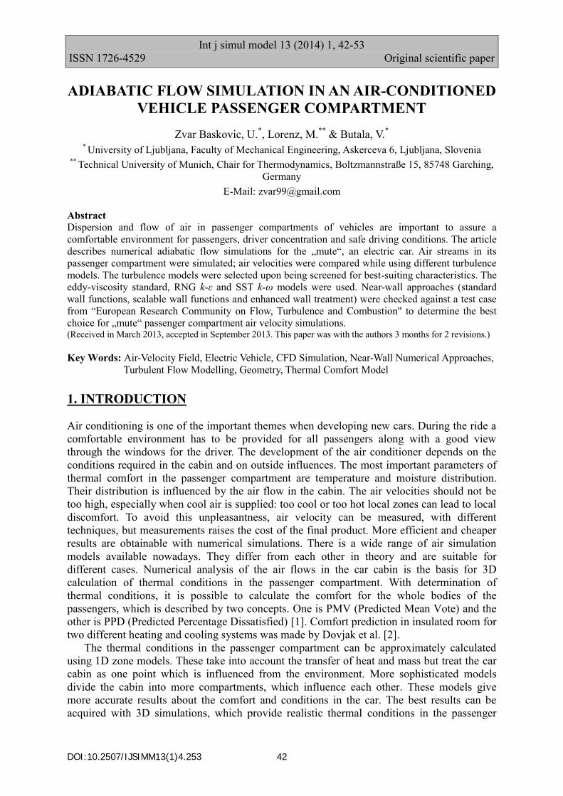
2.1 Standard k-ε model The standard k-ε model was developed by Launder and Spalding [13] and is today one of the most used models in simulating flows and heat transfer because of its reasonable accuracy for a wide range of turbulent flows. Many of simulations have been made and the standard k-ε model has been found to be very good in a wide range of situations. In a study with two ideal rooms [6] in which several one- and two-equation models were compared, the standard k–ε model provided good results, but its weakness is the presumption that the effect of molecular viscosity is negligible – and to satisfy this criterion the flow must be fully turbulent. 2.2 RNG k-ε model The re-normalization group (RNG) k-ε model includes a few refinements on the standard model and is therefore reliable for a wider range of flows. It is derived from Navier-Stokes equations using renormalization group methods. The model is thus capable of producing a more accurate prediction of flow in low Reynolds areas. The RNG turbulence model also provided good results when used for simulating indoor flows. 2.3 SST k-ω model The k-ω models are the most recent among two-equation eddy-viscosity turbulence models. The symbol ω represents the ratio of ε over k. There are two k-ω models available. The shear stress transport (SST) model was developed by Menter [14] and uses k-ω equations near wall boundaries and a transformed k- ε model far from walls, transitions being controlled by blending functions. 3. NEAR WALL TREATMENT DETERMINATION SIMULATION This chapter presents the numerical simulations that were carried out with the goal to determine best near-wall treatment approaches and eventually get the best results of air flow simulation in the „MUTE“ cabin. Our comparisons comprehended the enhanced wall treatment, standard wall functions and scalable wall functions on hexaeder meshes. The simulation results were compared with the experimental results found on the internet site of the European Research Community on Flow, Turbulence and Combustion, also known as ERCOFTAC: the simulated case has the title “Backward-Facing Step with Inclined Opposite Wall” [15]. The scheme of the experiment is depicted in Fig. 1 and parameters described in Table I. The software used for the simulations was developed by ANSYS, Inc. The meshing was performed in ANSYS ICEM CFD and the fluid simulations, in ANSYS Fluent. For all simulations in this paper,


45

pressure-based solver was used and for coupling between pressure and velocity SIMPLE scheme was used.

Figure 1: Scheme of the backward-facing step case [15].

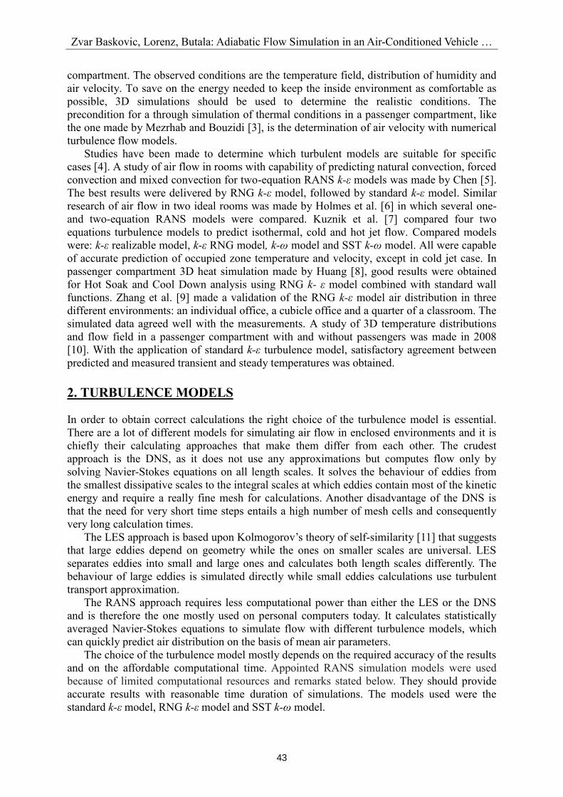
Table I: Tunnel geometry and inlet conditions [15].

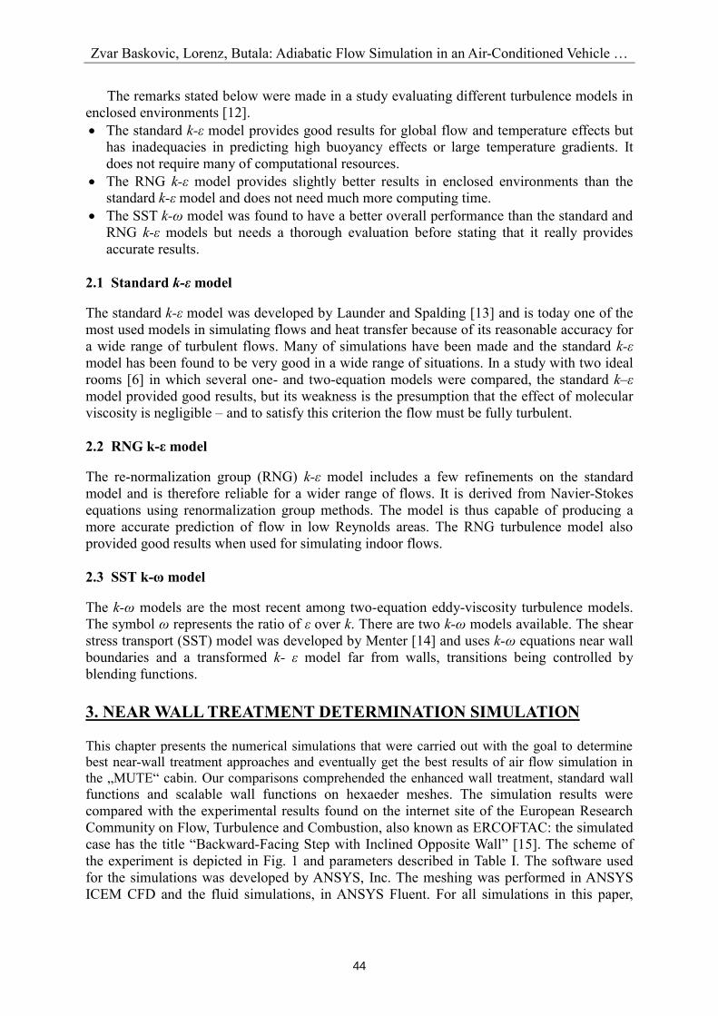
The inlet area was 1 m long, 15.1 cm wide and 10.1 cm high. The outlet was a step-height higher. The width of the tunnel was big enough to make it possible to neglect the influences of the side walls on the flow in the middle of the tunnel and to use two dimensional geometry. The ratio of the tunnel width to step height was 12. The inlet speed was 44.2 m/s. The near-wall treatment approaches compared were enhanced wall treatment, standard wall functions and scalable wall functions. The goal was to figure out whether they provide the same results for the same mesh. Velocity results in the x direction were compared at two vertical lines (y direction). The first one was 5.08 cm upstream of the step and the second one was 2.54 cm downstream of the step. Their positions are shown in Fig. 2.

Figure 2: Compared velocity positions. The simulation results were treated with Matlab software and compared with the experimental results, carried out by Driver and Seegmiller [15]. They are shown in Figs. 3a, 3b and 3c. In the simulations, the standard k-ε turbulence model in combination with standard wall functions was used. Momentum was discretized with second order upwind scheme and first order upwind scheme was applied for discretization of turbulent kinetic energy and turbulence dissipation rate equations.


46

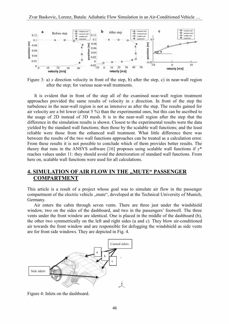
Figure 3: a) x direction velocity in front of the step, b) after the step, c) in near-wall region

after the step; for various near-wall treatments. It is evident that in front of the step all of the examined near-wall region treatment approaches provided the same results of velocity in x direction. In front of the step the turbulence in the near-wall region is not as intensive as after the step. The results gained for air velocity are a bit lower (about 5 %) than the experimental ones, but this can be ascribed to the usage of 2D instead of 3D mesh. It is in the near-wall region after the step that the difference in the simulation results is shown. Closest to the experimental results were the data yielded by the standard wall functions; then those by the scalable wall functions; and the least reliable were those from the enhanced wall treatment. What little difference there was between the results of the two wall functions approaches can be treated as a calculation error. From these results it is not possible to conclude which of them provides better results. The theory that runs in the ANSYS software [16] proposes using scalable wall functions if y* reaches values under 11: they should avoid the deterioration of standard wall functions. From here on, scalable wall functions were used for all calculations. 4. SIMULATION OF AIR FLOW IN THE „MUTE“ PASSENGER

COMPARTMENT This article is a result of a project whose goal was to simulate air flow in the passenger compartment of the electric vehicle „mute“, developed at the Technical University of Munich, Germany. Air enters the cabin through seven vents. There are three just under the windshield window, two on the sides of the dashboard, and two in the passengers’ footwell. The three vents under the front window are identical. One is placed in the middle of the dashboard (b), the other two symmetrically on the left and right sides (a and c). They blow air-conditioned air towards the front window and are responsible for defogging the windshield as side vents are for front side windows. They are depicted in Fig. 4.

Figure 4: Inlets on the dashboard.

a b c


47

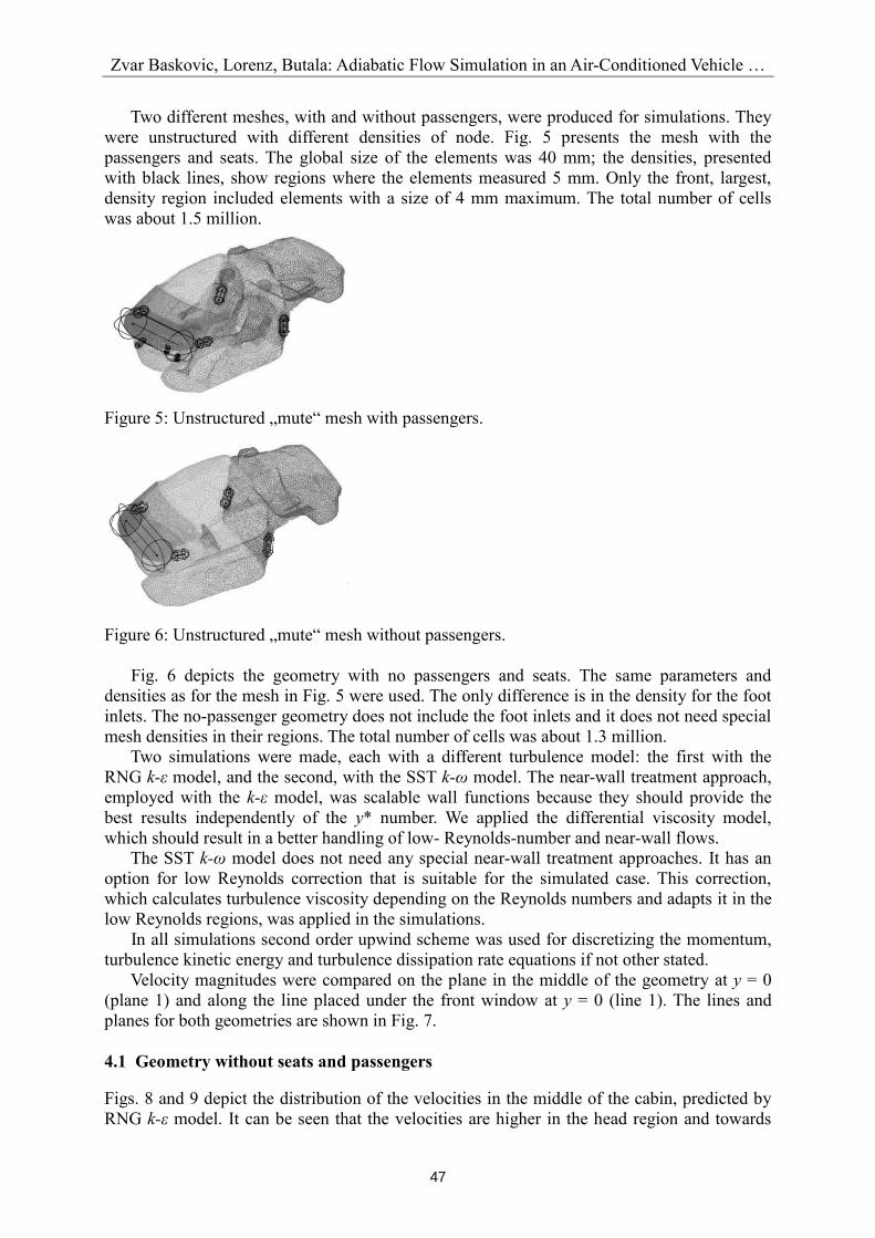
Two different meshes, with and without passengers, were produced for simulations. They were unstructured with different densities of node. Fig. 5 presents the mesh with the passengers and seats. The global size of the elements was 40 mm; the densities, presented with black lines, show regions where the elements measured 5 mm. Only the front, largest, density region included elements with a size of 4 mm maximum. The total number of cells was about 1.5 million.

Figure 5: Unstructured „mute“ mesh with passengers.

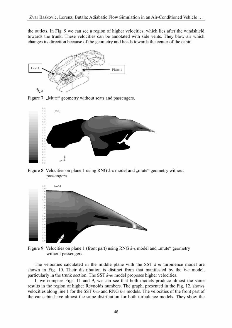
Figure 6: Unstructured „mute“ mesh without passengers. Fig. 6 depicts the geometry with no passengers and seats. The same parameters and densities as for the mesh in Fig. 5 were used. The only difference is in the density for the foot inlets. The no-passenger geometry does not include the foot inlets and it does not need special mesh densities in their regions. The total number of cells was about 1.3 million. Two simulations were made, each with a different turbulence model: the first with the RNG k-ε model, and the second, with the SST k-ω model. The near-wall treatment approach, employed with the k-ε model, was scalable wall functions because they should provide the best results independently of the y* number. We applied the differential viscosity model, which should result in a better handling of low- Reynolds-number and near-wall flows. The SST k-ω model does not need any special near-wall treatment approaches. It has an option for low Reynolds correction that is suitable for the simulated case. This correction, which calculates turbulence viscosity depending on the Reynolds numbers and adapts it in the low Reynolds regions, was applied in the simulations. In all simulations second order upwind scheme was used for discretizing the momentum, turbulence kinetic energy and turbulence dissipation rate equations if not other stated. Velocity magnitudes were compared on the plane in the middle of the geometry at y = 0 (plane 1) and along the line placed under the front window at y = 0 (line 1). The lines and planes for both geometries are shown in Fig. 7. 4.1 Geometry without seats and passengers Figs. 8 and 9 depict the distribution of the velocities in the middle of the cabin, predicted by RNG k-ε model. It can be seen that the velocities are higher in the head region and towards


48

the outlets. In Fig. 9 we can see a region of higher velocities, which lies after the windshield towards the trunk. These velocities can be annotated with side vents. They blow air which changes its direction because of the geometry and heads towards the center of the cabin.

Figure 7: „Mute“ geometry without seats and passengers.

Figure 8: Velocities on plane 1 using RNG k-ε model and „mute“ geometry without

passengers.

Figure 9: Velocities on plane 1 (front part) using RNG k-ε model and „mute“ geometry

without passengers. The velocities calculated in the middle plane with the SST k-ω turbulence model are shown in Fig. 10. Their distribution is distinct from that manifested by the k-ε model, particularly in the trunk section. The SST k-ω model proposes higher velocities. If we compare Figs. 11 and 9, we can see that both models produce almost the same results in the region of higher Reynolds numbers. The graph, presented in the Fig. 12, shows velocities along line 1 for the SST k-ω and RNG k-ε models. The velocities of the front part of the car cabin have almost the same distribution for both turbulence models. They show the

[m/s]

[m/s]


49

peak velocity (about 1.5 m/s) above the defrosting vents. On both sides the velocity magnitude declines sharply. There is another peak where x reaches 0.05 m. It originates from the eddy which is produced on the front side of the vents.

Figure 10: Velocities on the plane 1 using SST k-ω model and „mute“ geometry without

passengers.

Figure 11: Velocities on the plane 1 (front part) using SST k-ω model and „mute“ geometry without passengers.

Figure 12: Air velocity along line 1 using SST k-ω model and RNG k-ε model on „mute“

geometry without passengers. Both air velocity distributions (from RNG k-ε and SST k-ω models) seem to be plausible. The biggest difference can be seen in the air velocity distribution in the front part of the trunk, where the SST k-ω model proposed up to four times higher velocities than the RNG k-ε

[m/s]

[m/s]


50

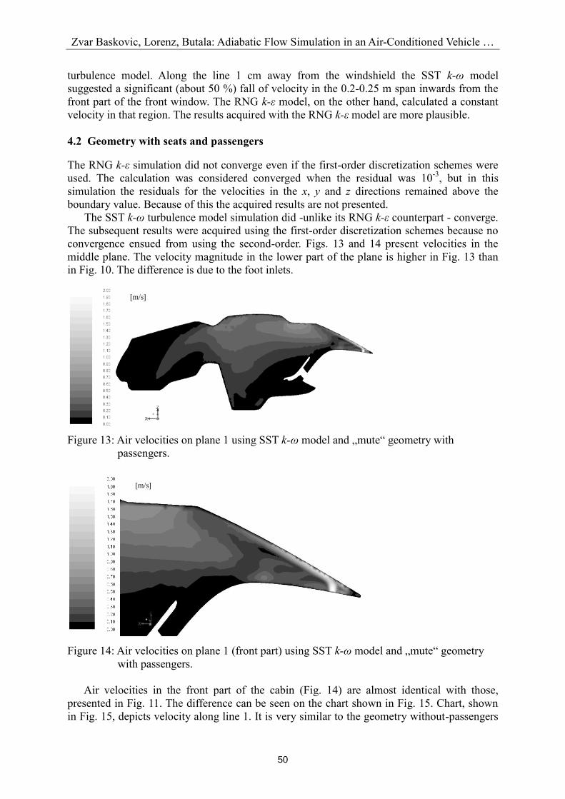
turbulence model. Along the line 1 cm away from the windshield the SST k-ω model suggested a significant (about 50 %) fall of velocity in the 0.2-0.25 m span inwards from the front part of the front window. The RNG k-ε model, on the other hand, calculated a constant velocity in that region. The results acquired with the RNG k-ε model are more plausible. 4.2 Geometry with seats and passengers The RNG k-ε simulation did not converge even if the first-order discretization schemes were used. The calculation was considered converged when the residual was 10-3, but in this simulation the residuals for the velocities in the x, y and z directions remained above the boundary value. Because of this the acquired results are not presented. The SST k-ω turbulence model simulation did -unlike its RNG k-ε counterpart - converge. The subsequent results were acquired using the first-order discretization schemes because no convergence ensued from using the second-order. Figs. 13 and 14 present velocities in the middle plane. The velocity magnitude in the lower part of the plane is higher in Fig. 13 than in Fig. 10. The difference is due to the foot inlets.

Figure 13: Air velocities on plane 1 using SST k-ω model and „mute“ geometry with

passengers.

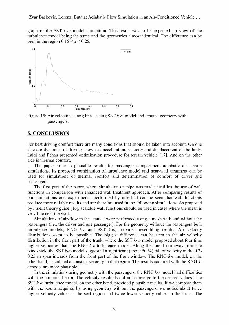
Figure 14: Air velocities on plane 1 (front part) using SST k-ω model and „mute“ geometry

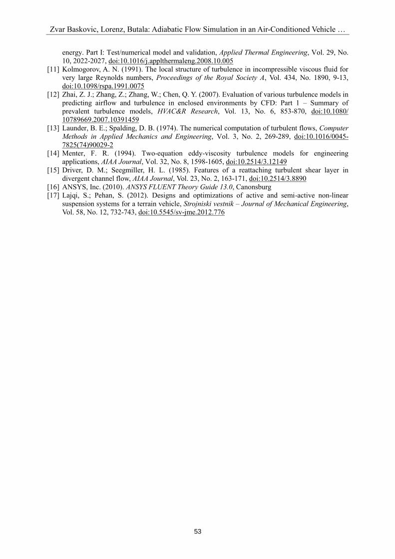
with passengers. Air velocities in the front part of the cabin (Fig. 14) are almost identical with those, presented in Fig. 11. The difference can be seen on the chart shown in Fig. 15. Chart, shown in Fig. 15, depicts velocity along line 1. It is very similar to the geometry without-passengers

[m/s]

[m/s]


51

graph of the SST k-ω model simulation. This result was to be expected, in view of the turbulence model being the same and the geometries almost identical. The difference can be seen in the region 0.15 < x < 0.25.

Figure 15: Air velocities along line 1 using SST k-ω model and „mute“ geometry with

passengers. 5. CONCLUSION For best driving comfort there are many conditions that should be taken into account. On one side are dynamics of driving shown as acceleration, velocity and displacement of the body. Lajqi and Pehan presented optimization procedure for terrain vehicle [17]. And on the other side is thermal comfort. The paper presents plausible results for passenger compartment adiabatic air stream simulations. Its proposed combination of turbulence model and near-wall treatment can be used for simulations of thermal comfort and determination of comfort of driver and passengers. The first part of the paper, where simulation on pipe was made, justifies the use of wall functions in comparison with enhanced wall treatment approach. After comparing results of our simulations and experiments, performed by insert, it can be seen that wall functions produce more reliable results and are therefore used in the following simulations. As proposed by Fluent theory guide [16], scalable wall functions should be used in cases where the mesh is very fine near the wall. Simulations of air-flow in the „mute“ were performed using a mesh with and without the passengers (i.e., the driver and one passenger). For the geometry without the passengers both turbulence models, RNG k-ε and SST k-ω, provided resembling results. Air velocity distributions seem to be possible. The biggest difference can be seen in the air velocity distribution in the front part of the trunk, where the SST k-ω model proposed about four time higher velocities than the RNG k-ε turbulence model. Along the line 1 cm away from the windshield the SST k-ω model suggested a significant (about 50 %) fall of velocity in the 0.2-0.25 m span inwards from the front part of the front window. The RNG k-ε model, on the other hand, calculated a constant velocity in that region. The results acquired with the RNG k-ε model are more plausible. In the simulations using geometry with the passengers, the RNG k-ε model had difficulties with the numerical error. The velocity residuals did not converge to the desired values. The SST k-ω turbulence model, on the other hand, provided plausible results. If we compare them with the results acquired by using geometry without the passengers, we notice about twice higher velocity values in the seat region and twice lower velocity values in the trunk. The


52

former difference originates from the air inlets in the foot region. The latter, from the presence of the driver and the passenger: these two present an obstacle to the air. Velocity magnitude along the line under the windshield falls more continuously than when using geometry without the passengers. This article presents beginning of the three dimensional thermal comfort model. Air velocity distributions, acquired with simulations should represent actual conditions in the passenger compartment and they present basis for further calculations of temperature and moisture distributions. First, simulations should be validated with one measuring method or combination of them. Probably would be the most suitable method PIV (Particle Image Velocity) because it would be possible to set it this way that it would have no influence on the flow in the cabin. In the case of too big differences in simulated and measured velocities, should be used some other turbulence models, which are suitable for low-Reynolds number flows. It would be possible to use turbulence models, which demand more computing power, if appropriate computers would be available. Also temperature and moisture distribution in the cabin should be simulated and validated. From the acquired data it would be possible to calculate thermal comfort in the passenger compartment. This is the basis for adaptations of air conditioning in the car to assure best thermal conditions for the passengers. 6. ACKNOWLEDGEMENT The authors would like to thank the Likar Foundation for financial support. REFERENCES [1] Standard SIST EN ISO 7730 (2005). Ergonomics of the thermal environment – Analytical

determination and interpretation of thermal comfort using calculation of the PMV and PPD indices and local thermal comfort criteria, Geneve

[2] Dovjak, M.; Shukuya, M.; Krainer, A. (2012). Exergy analysis of conventional and low exergy systems for heating and cooling of near zero energy buildings, Strojniski vestnik – Journal of Mechanical Engineering, Vol. 58, No. 7-8, 453-461, doi:10.5545/sv-jme.2011.158

[3] Mezrhab, A.; Bouzidi, M. (2006). Computation of thermal comfort inside a passenger car compartment, Applied Thermal Engineering, Vol. 26, No. 14-15, 1697-1704, doi:10.1016/ j.applthermaleng.2005.11.008

[4] Novak, D.; Radisic, T.; Alfirevic, I. (2012). Determining the influence of outside air temperature on aircraft airspeed, Transactions of FAMENA, Vol. 36, No. 3, 45-54

[5] Chen, Q. (1995). Comparison of different k-e models for indoor air flow computations, Numerical Heat Transfer, Part B: Fundamentals: An International Journal of Computation and Methodology, Vol. 28, No. 3, 353-369, doi:10.1080/10407799508928838

[6] Holmes, S. A.; Jouvray, A.; Tucker, P. G. (2000). An assessment of a range of turbulence models when predicting room ventilation, Proceedings of Healthy Buildings, Vol. 2, 401-406

[7] Kuznik, F.; Rusaouen, G.; Brau, J. (2007). Experimental and numerical study of a full scale ventilated enclosure: Comparison of four two equation closure turbulence models, Building and Environment, Vol. 42, No. 3, 1043-1053, doi:10.1016/j.buildenv.2005.11.024

[8] Huang, L.; Han, T. (2002). Validation of 3-D passenger compartment hot soak and cool-down analysis for virtual thermal comfort engineering, SAE Technical Paper 2002-01-1304, SAE 2002 World Congress & Exhibition, doi:10.4271/2002-01-1304

[9] Zhang, L.; Chow, T. T.; Wang, Q.; Fong, K. F.; Chan, L. S. (2005). Validation of CFD model for research into displacement ventilation, Architectural Science Review, Vol. 48, No. 4, 305-316, doi:10.3763/asre.2005.4838

[10] Zhang, H.; Dai, L.; Xu, G.; Li, Y.; Chen, W.; Tao, W.-Q. (2009). Studies of air-flow and temperature fields inside a passenger compartment for improving thermal comfort and saving

http://dx.doi.org/10.5545/sv-jme.2011.158

http://dx.doi.org/10.1016/j.applthermaleng.2005.11.008


http://dx.doi.org/10.1080/10407799508928838

http://dx.doi.org/10.1016/j.buildenv.2005.11.024

http://dx.doi.org/10.4271/2002-01-1304

http://dx.doi.org/10.3763/asre.2005.4838


53

energy. Part I: Test/numerical model and validation, Applied Thermal Engineering, Vol. 29, No. 10, 2022-2027, doi:10.1016/j.applthermaleng.2008.10.005

[11] Kolmogorov, A. N. (1991). The local structure of turbulence in incompressible viscous fluid for very large Reynolds numbers, Proceedings of the Royal Society A, Vol. 434, No. 1890, 9-13, doi:10.1098/rspa.1991.0075

[12] Zhai, Z. J.; Zhang, Z.; Zhang, W.; Chen, Q. Y. (2007). Evaluation of various turbulence models in predicting airflow and turbulence in enclosed environments by CFD: Part 1 – Summary of prevalent turbulence models, HVAC&R Research, Vol. 13, No. 6, 853-870, doi:10.1080/ 10789669.2007.10391459

[13] Launder, B. E.; Spalding, D. B. (1974). The numerical computation of turbulent flows, Computer Methods in Applied Mechanics and Engineering, Vol. 3, No. 2, 269-289, doi:10.1016/0045-7825(74)90029-2

[14] Menter, F. R. (1994). Two-equation eddy-viscosity turbulence models for engineering applications, AIAA Journal, Vol. 32, No. 8, 1598-1605, doi:10.2514/3.12149

[15] Driver, D. M.; Seegmiller, H. L. (1985). Features of a reattaching turbulent shear layer in divergent channel flow, AIAA Journal, Vol. 23, No. 2, 163-171, doi:10.2514/3.8890

[16] ANSYS, Inc. (2010). ANSYS FLUENT Theory Guide 13.0, Canonsburg [17] Lajqi, S.; Pehan, S. (2012). Designs and optimizations of active and semi-active non-linear

suspension systems for a terrain vehicle, Strojniski vestnik – Journal of Mechanical Engineering, Vol. 58, No. 12, 732-743, doi:10.5545/sv-jme.2012.776


http://dx.doi.org/10.1098/rspa.1991.0075

http://dx.doi.org/10.1080/10789669.2007.10391459

http://dx.doi.org/10.1080/10789669.2007.10391459

http://dx.doi.org/10.1016/0045-7825(74)90029-2

http://dx.doi.org/10.1016/0045-7825(74)90029-2

http://dx.doi.org/10.2514/3.12149

http://dx.doi.org/10.2514/3.8890

http://dx.doi.org/10.5545/sv-jme.2012.776

adiabatic flow simulation in an air conditioned vehicle passenger compartment · 2015-03-09 ·...

Documents