Adjoint Models as Analytical Tools

Dr. Ronald M. Errico

Goddard Earth Sciences and Technology Center (UMBC) Global Modeling and Assimilation Office (NASA)

Outline

1. Sensitivity analysis: The basis for adjoint model applications2. Examples of adjoint-derived sensitivity3. Code construction: an example4. Nonlinear validation5. Efficient solution of optimization problems6. Adjoint models as paradigm changers7. Singular vectors8. Observation sensitivity9. Other applications10. Other considerations11. Summary

Sensitivity Analysis: The basis for adjoint model applications

Impacts vs. Sensitivity

xi

xj

A single impact study yields exact response measures (J) for all forecast aspects with respect to the particular perturbation investigated.

A single adjoint-derived sensitivity yields linearized estimates of the particular measure (J) investigated with respect to all possible perturbations.

Adjoint Sensitivity Analysis Impacts vs. Sensitivities

Examples of Adjoint-Derived Sensitivities

Contour interval 0.02 Pa/m M=0.1 Pa/m

Example Sensitivity Field

Errico andVukicevic1992 MWR

Lewis et al. 2001

From Errico and Vukicevic 1992

J=average surface pressure in a small box centered at P

J=barotropic component of vorticity at point P

Development of Adjoint Model From Line by Line Analysis of Computer Code

Development of Adjoint Model From Line by Line Analysis of Computer Code

Y = X * (W**A)Z = Y * X

Ytlm = Xtlm * (W**A) + Wtlm *A* X *(W**(A-1))Ztlm = Ytlm * X + Xtlm * Y

Xadj = Xadj + Zadj * YYadj = Yadj + Zadj * X

Xadj = Xadj + Yadj * (W**A) Wadj = Wadj + Yadj * X *(W**(A-1))

Development of Adjoint Model From Line by Line Analysis of Computer Code

Parent NLM :

TLM :

Adjoint :

Y = X * (W**A)Z = Y * X

Ytlm = Xtlm * (W**A) + Wtlm *A* X *(W**(A-1))Ztlm = Ytlm * X + Xtlm * Y

Xadj = Xadj + Zadj * YYadj = Yadj + Zadj * X

Xadj = Xadj + Yadj * (W**A) Wadj = Wadj + Yadj * X *(W**(A-1))

Development of Adjoint Model From Line by Line Analysis of Computer Code

Parent NLM :

TLM :

Adjoint :

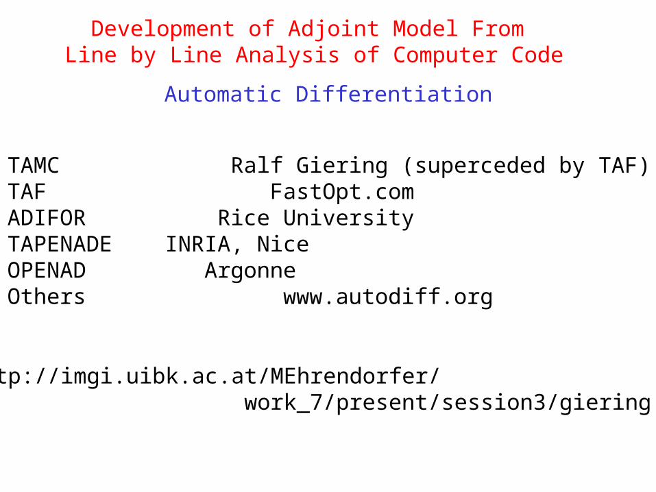
Development of Adjoint Model From Line by Line Analysis of Computer Code

Automatic Differentiation

TAMC Ralf Giering (superceded by TAF)TAF FastOpt.comADIFOR Rice UniversityTAPENADE INRIA, NiceOPENAD ArgonneOthers www.autodiff.org

See http://imgi.uibk.ac.at/MEhrendorfer/ work_7/present/session3/giering.pdf

Development of Adjoint Model From Line by Line Analysis of Computer Code

1. TLM and Adjoint models are straight-forward to derive from NLM code, and actually simpler to develop. 2. Intelligent approximations can be made to improve efficiency. 3. TLM and (especially) Adjoint codes are simple to test

rigorously.4. Some outstanding errors and problems in the NLM are typically revealed when the TLM and Adjoint are developed from it.5. It is best to start from clean NLM code.6. The TLM and Adjoint can be formally correct but useless!

Nonlinear Validation

Does the TLM or Adjoint model tell us anything aboutthe behavior of meaningful perturbations in the nonlinearmodel that may be of interest?

Linear vs. Nonlinear Results in Moist Model

24-hour SV1 from case W1 Initialized with T’=1K Final ps field shown

Contour interval 0.5 hPa

Errico and Raeder1999 QJRMS

Non-ConvPrecip. ci=0.5mm

ConvectivePrecip. ci=2mm

ConvectivePrecip. ci=2mm

Non-ConvPrecip. ci=0.5mm

Linear vs. Nonlinear Results in Moist Model

Non-Convective

Convective.

Comparison of TLM and Nonlinearly Produced Precip Rates 12-Hour Forecasts with SV#1

Errico et al.QJRMS 2004

Linear

Linear

Nonlinear

Nonlinear

Contours: 0.1, 0.3, 1., 3., 10. mm/day

Linear vs. Nonlinear Results

In general, agreement between TLM and NLM resultswill depend on:

1. Amplitude of perturbations2. Stability properties of the reference state3. Structure of perturbations4. Physics involved5. Time period over which perturbation evolves6. Measure of agreement

The agreement of the TLM and NLM is exactlythat of the Adjoint and NLM if the Adjoint is exactwith respect to the TLM.

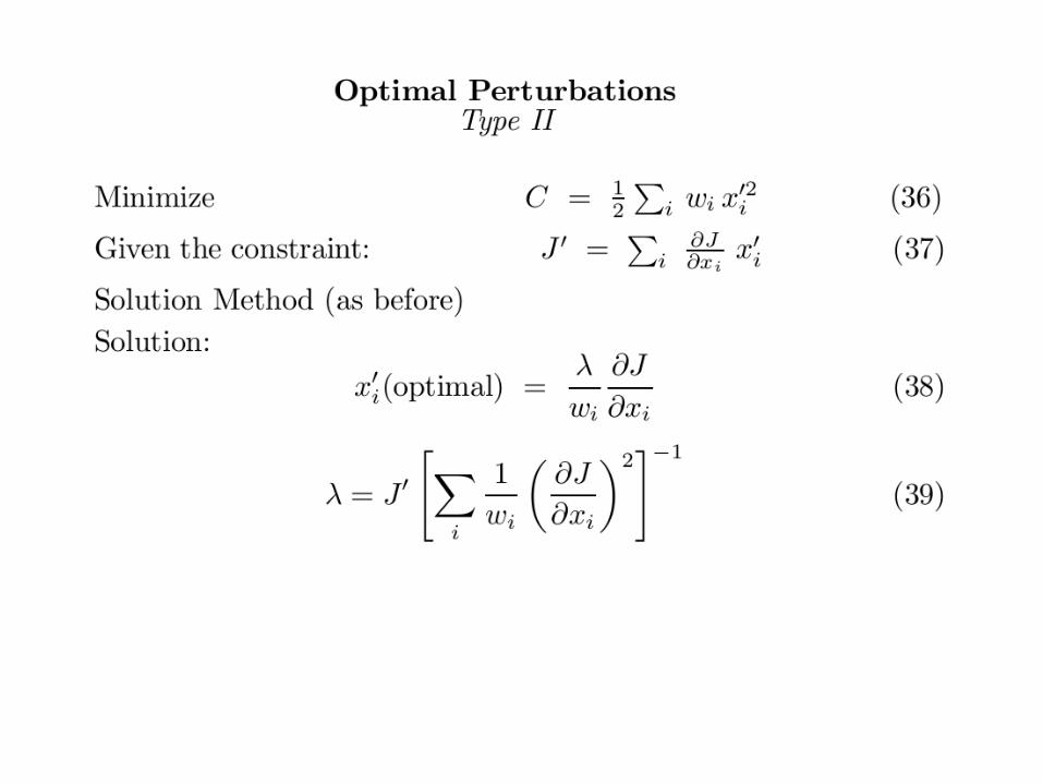
Efficient solution of optimization problems

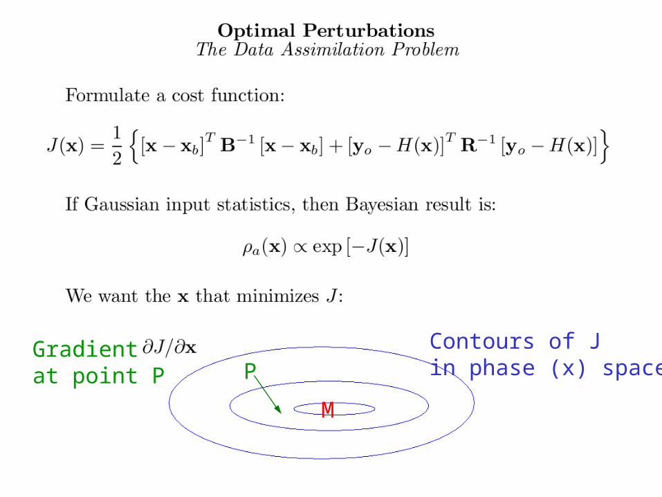
M

Contours of Jin phase (x) spaceP

Gradient at point P

Adjoint models as paradigm changers

Sensitivity field for J=ps with respect to T for an idealized cyclone

From Langland and Errico 1996 MWR

100hPa

1000hPa

500hPa

Contour 0.1 unit Contour 1.0 unit

Adjoint of Nudging Fields

Bao and Errico: MWR 1997

t=0

t=48 hours

Errico et al.Tellus 1993

0.4 units

5.0 units

Non-Convective Forecast Precipitation Rate

Contour interval 2 cm/day

Errico, Raeder, Fillion: 2003 Tellus

What is the modeled precipitation rate sensitive to?

Errico et al.2003 Tellus

Impacts for adjoint-derived optimalperturbations forforecasts startingindicated hours in the past.

Vort optimized

Rc optimized Rn Optimized

Errico et al. QJRMS 2004

Initial u, v, T, ps Perturbation Initial q Perturbation

12-hour v TLM forecasts

Perturbations in Different Fields Can Produce the Same Result

Singular Vectors

Gelaro et al.MWR 2000

Bred Modes (LVs)And SVs

Gelaro et al. QJRMS 2002

Results for Leading 10 SVs

Vertical modes of the 10-level MAMS model(from Errico, 2000 QJRMS)

m102161 H

m20602 H

m147 H

Balance of Singular Vectors

Errico 2000

Balance of Singular Vectors

t=0 t=24 hours

E=E_t, K=KE, A=APE, R=R mode E, G=G mode E

A,G E,K,R

The Balance of Singular Vectors

)55.0(T

InitialR mode

InitialG mode

Contour2 units

Contour1 unit

Errico 2000

)55.0(v

SingularValueSquared

Mode Index

Errico et al.Tellus 2001

EM E-norm Moist ModelED E-norm Dry ModelTM R-norm Moist ModelTD R-norm Dry Model

How Many SVs are Growing Ones?

From Novakovskaia et al. 2007 and Errico et al. 2007

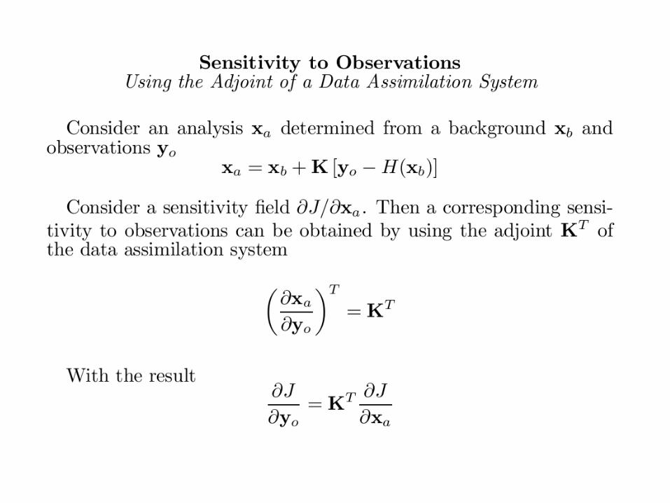
Sensitivity to Observations The use of an adjoint of a data analysis algorithm

Sensitivity to analyzed potential temperature at 500 hPa

Sensitivity to raob temperatures at 500 hPa

From Gelaroand Zhu 2006

J = mean squared24 hour forecasterror using E-norm

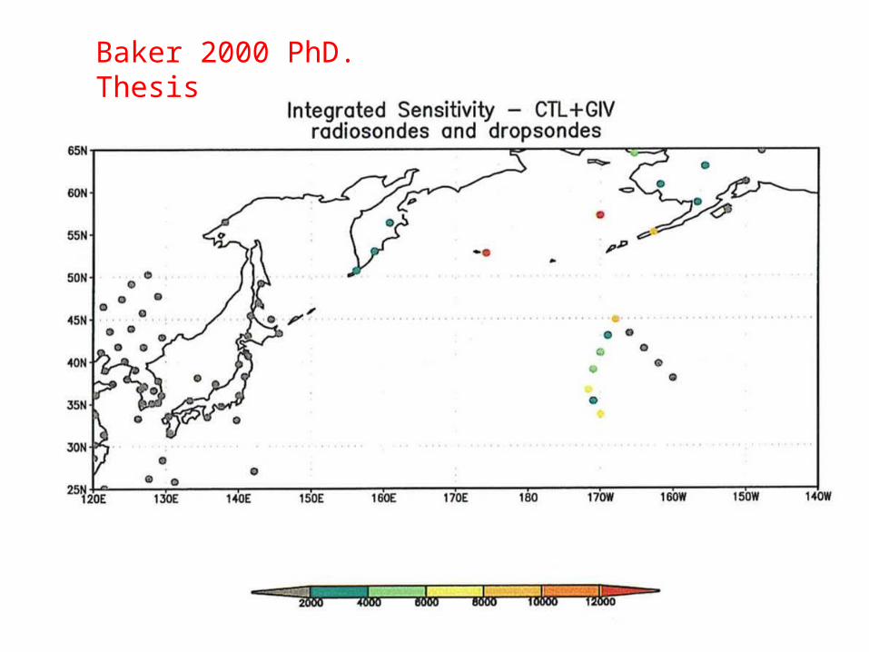
Baker 2000 PhD. Thesis

-20

-15

-10

-5

0

5

10

15

-20

-15

-10

-5

0

5

10

15

(J/Kg)e

…all observing systems provide

total monthly benefit

Impacts of various observing systems TotalsGEOS-5 July 2005

0e

Observation Count (millions)

Observation Count (millions)

(J/Kg)e 0e

NH observations

SH observations

From R. Gelaro

AMSU-A (15 ch) AIRS (153 ch)

H2O Channels

Diagnosing impact of hyper-spectral observing systemsC

hann

el

Cha

nnel

(J/Kg) Forecast Error Reduction (J/Kg)

GEOS-5 July 2005 00z Totals

Forecast degradation

e (J/Kg)e-0.6-7.0

…some AIRS water vapor channels currently degrade the 24h forecast in GEOS-5…

0 0

From R. Gelaro

Other Applications

1. 4DVAR (P. Courtier)2. Ensemble Forecasting (R. Buizza, T. Palmer)3. Key analysis errors (F. Rabier, L. Isaksen)4. Targeting (R. Langland, R. Gelaro)

Problems with Physics

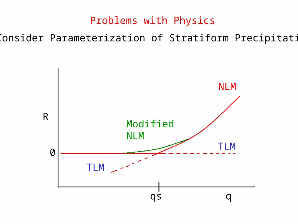
Problems with Physics

Consider Parameterization of Stratiform Precipitation

R

0

qqs

NLM

TLM

TLM

ModifiedNLM

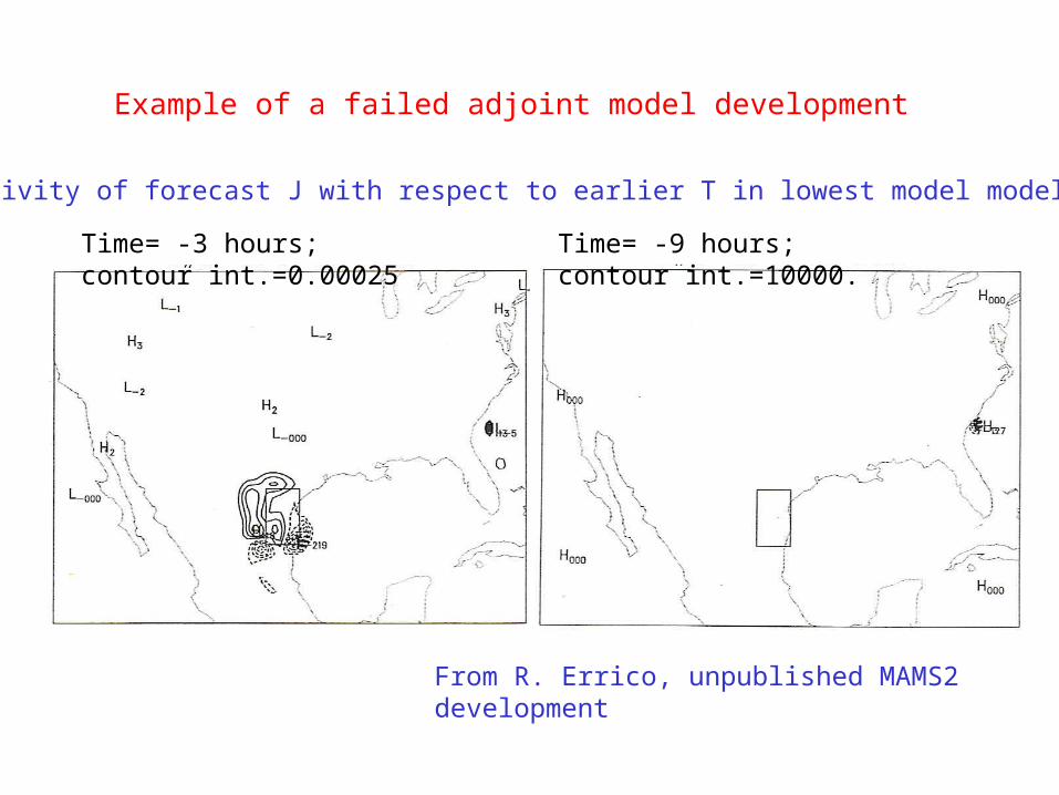
Sensitivity of forecast J with respect to earlier T in lowest model model level

Time= -3 hours; contour int.=0.00025 Time= -9 hours; contour int.=10000.

From R. Errico, unpublished MAMS2 development

Example of a failed adjoint model development

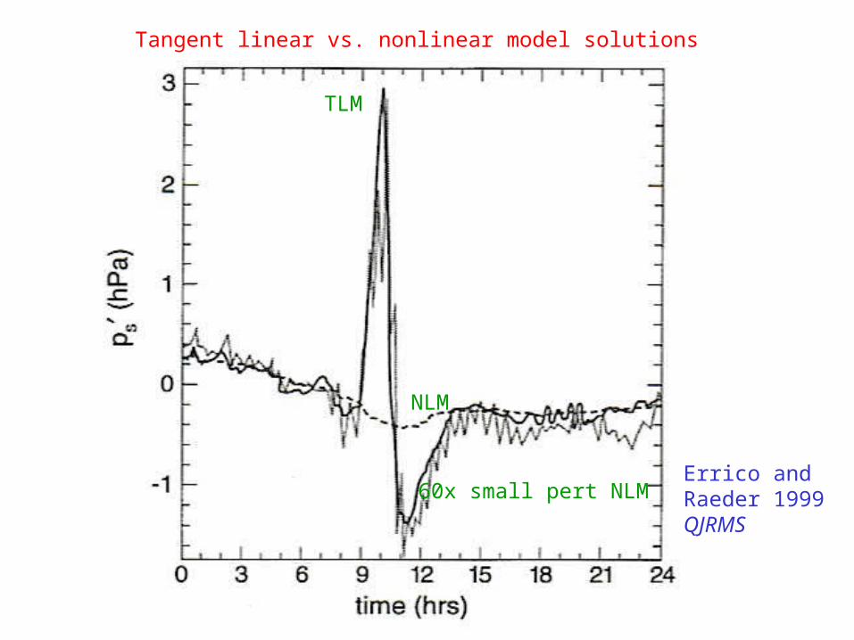
Tangent linear vs. nonlinear model solutions

Errico andRaeder 1999QJRMS

TLM

60x small pert NLM

NLM

RAS scheme

ECMWF scheme

BM scheme

Fillion and Mahfouf 1999 MWR

Jacobians of Precipitation

Problems with Physics

1. The model may be non-differentiable.2. Unrealistic discontinuities should be smoothed after reconsideration of the physics being parameterized.3. Perhaps worse than discontinuities are numerical insta- bilities that can be created from physics linearization.4. It is possible to test the suitability of physics components for adjoint development before constructing the adjoint.5. Development of an adjoint provides a fresh and complementary look at parameterization schemes.

Other Considerations

Physically-based norms and the interpretations ofsensitivity fields

Sensitivity of J with respect to u 5 days earlier at 45ON, where J is the zonal mean of zonal wind within a narrow band centered on 10 hPa and 60ON. (From E. Novakovskaia)

10 hPa

0.1 hPa

1000 hPa

100 hPa

1 hPa

- 180 + 180 0 Longitude

Continuous vs. grid-point representations of sensitivity

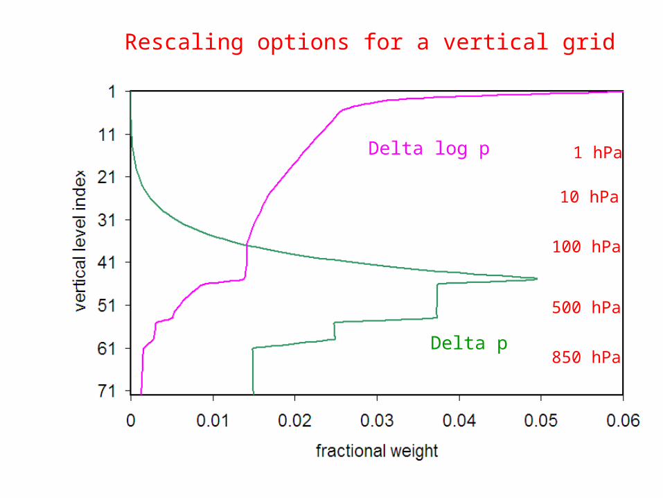
Rescaling options for a vertical grid

Delta log p

Delta p

500 hPa

100 hPa

10 hPa

1 hPa

850 hPa

1000 hPa

10 hPa

0.1 hPa

Mass weighting Volume weighting

2 Re-scalings of the adjoint results

From E. Novakovskaia

Summary

Unforeseen Results Leading to New Paradigms

1. Atmospheric flows are very sensitive to low-level T perturbations.2. Evolution of a barotropic flow can be very sensitive to perturbations having small vertical scale.3. Error structures can propagate and amplify rapidly. 4. Forecast barotropic vorticity can be sensitive to initial water vapor. 5. When significant R is present, moist enthalpy appears a key field.6. Nudging has strange properties.7. Relatively few perturbation structures are initially growing ones.8. Sensitivities to observations differ from sensitivities to analyses.9. A TLM including physics can be useful.

Misunderstanding #1

False: Adjoint models are difficult to understand. True: Understanding of adjoints of numerical models primarily requires concepts taught in early college mathematics.

Misunderstanding #2

False: Adjoint models are difficult to develop. True: Adjoint models of dynamical cores are simpler to develop than their parent models, and almost trivial to check, but adjoints of model physics can pose difficult problems.

Misunderstanding #3

False: Automatic adjoint generators easily generate perfect and useful adjoint models.

True: Problems can be encountered with automatically generated adjoint codes that are inherent in the parent model. Do these problems also have a bad effect in the parent model?

Misunderstanding #4

False: An adjoint model is demonstrated useful and correct if it reproduces nonlinear results for ranges of very small perturbations. True: To be truly useful, adjoint results must yield good approximations to sensitivities with respect to meaningfully large perturbations. This must be part of the validation process.

Misunderstanding #5

False: Adjoints are not needed because the EnKF is better than 4DVAR and adjoint results disagree with our notions of atmospheric behavior. True: Adjoint models are more useful than just for 4DVAR. Their results are sometimes profound, but usually confirmable, thereby requiring new theories of atmospheric behavior. It is rare that we have a tool that can answer such important questions so directly!

What is happening and where are we headed?

1. There are several adjoint models now, with varying portions of physics and validation.2. Utilization and development of adjoint models has been slow to expand, for a variety of reasons.3. Adjoint models are powerful tools that are under-utilized.4. Adjoint models are like gold veins waiting to be mined.

Recommendations

1. Develop adjoint models.2. Include more physics in adjoint models.3. Develop parameterization schemes suitable for linearized applications.4. Always validate adjoint results (linearity).4. Consider applications wherever sensitivities would be useful.

Adjoint Workshop

The 8th will be in fall2008 or spring 2009.

Contact Dr. R. Erricorerrico@gmao.gsfc.nasa.govto be put on mailing list