CHAPTER 15Firm Valuation: Cost of Capital and

Adjusted Present Value Approaches

The preceding two chapters examined two approaches to valuing the equity in thefirm—the dividend discount model and the free cash flow to equity (FCFE) valu-

ation model. This chapter develops another approach to valuation where the entirefirm is valued, by either discounting the cumulated cash flows to all claim holdersin the firm by the weighted average cost of capital (the cost of capital approach) orby adding the marginal impact of debt on value to the unlevered firm value—theadjusted present value (APV) approach).

In the process of looking at firm valuation, we also look at how leverage mayor may not affect firm value. We note that in the presence of default risk, taxes, andagency costs, increasing leverage can sometimes increase firm value and sometimesdecrease it. In fact, we argue that the optimal financing mix for a firm is the onethat maximizes firm value.

FREE CASH FLOW TO THE FIRM

The free cash flow to the firm (FCFF) is the sum of the cash flows to all claim hold-ers in the firm, including stockholders, bondholders, and preferred stockholders.There are two ways of measuring the free cash flow to the firm.

One is to add up the cash flows to the claim holders, which would includecash flows to equity (defined either as free cash flow to equity or dividends), cashflows to lenders (which would include principal payments, interest expenses, andnew debt issues), and cash flows to preferred stockholders (usually preferred dividends):

FCFF = Free cash flow to equity + Interest expense(1 − Tax rate) + Principal repayments − New debt issues + Preferred dividends

Note, however, that we are reversing the process that we used to get to free cashflow to equity, where we subtracted out payments to lenders and preferred stock-holders to estimate the cash flow left for stockholders. A simpler way of gettingto free cash flow to the firm is to estimate the cash flows prior to any of theseclaims. Thus we could begin with the earnings before interest and taxes, net out

380

ch15_p380_422.qxd 12/5/11 2:15 PM Page 380

taxes and reinvestment needs, and arrive at an estimate of the free cash flow tothe firm:

FCFF = EBIT(1 − Tax rate) + Depreciation − Capital expenditure − Δ Working capital

Since this cash flow is prior to debt payments, it is often referred to as an unleveredcash flow. Note that this free cash flow to the firm does not incorporate any of thetax benefits due to interest payments. This is by design, because the use of the after-tax cost of debt in the cost of capital already considers this benefit, and including itin the cash flows would double count it.

FCFF and Other Cash Flow Measures

The differences between FCFF and FCFE arise primarily from cash flows associatedwith debt—interest payments, principal repayments, and new debt issues—andother nonequity claims, such as preferred dividends. For firms at their desired debtlevel, which finance their capital expenditures and working capital needs with thismix of debt and equity and use debt issues to finance principal repayments, the freecash flow to the firm will exceed the free cash flow to equity.

One measure that is widely used in valuation is the earnings before interest,taxes, depreciation, and amortization (EBITDA). The free cash flow to the firm is a closely related concept but it takes into account the potential tax liabil-ity from the earnings as well as capital expenditures and working capital requirements.

Three measures of earnings are also often used to derive cash flows. Theamount of earnings before interest and taxes (EBIT) or operating income comes di-rectly from a firm’s income statements. Adjustments to EBIT yield the net operatingprofit or loss after taxes (NOPLAT) or the net operating income (NOI). The net op-erating income is defined to be the income from operations prior to taxes and non-operating expenses.

Each of these measures is used in valuation models, and each can be related tothe free cash flow to the firm. Each, however, makes some assumptions about therelationship between depreciation and capital expenditures that are made explicitin Table 15.1.

Growth in FCFE versus Growth in FCFF

Will equity cash flows and firm cash flows grow at the same rate? Consider thestarting point for the two cash flows. Equity cash flows are based on net income orearnings per share—measures of equity income. Firm cash flows are based on oper-ating income (i.e., income prior to debt payments). As a general rule, you would ex-pect growth in operating income to be lower than growth in net income, becausefinancial leverage can augment the latter. To see why, let us go back to the funda-mental growth equations laid out in Chapter 11:

Expected growth in net income = Equity reinvestment rate × Return on equity

Expected growth in operating income = Reinvestment rate × Return on capital

Free Cash Flow to the Firm 381

ch15_p380_422.qxd 12/5/11 2:15 PM Page 381

We also defined the return on equity in terms of the return on capital:

When a firm borrows money and invests in projects that earn more than the after-tax cost of debt, the return on equity will be higher than the return on capital.This, in turn, will translate into a higher growth rate in equity income at least inthe short term.

In stable growth, though, the growth rates in equity income and operating in-come have to converge. To see why, assume that you have a firm whose revenuesand operating income and growing at 5 percent a year forever. If you assume thatthe same firm’s net income grows at 6 percent a year forever, the net income willcatch up with operating income at some point in time in the future and exceed rev-enues at a later point in time. In stable growth, therefore, even if return on equity

Return on equity Return on capitalDebt

Equity

(Return on capital After-tax cost of debt)

= +

× −

382 FIRM VALUATION: COST OF CAPITAL AND ADJUSTED PRESENT VALUE APPROACHES

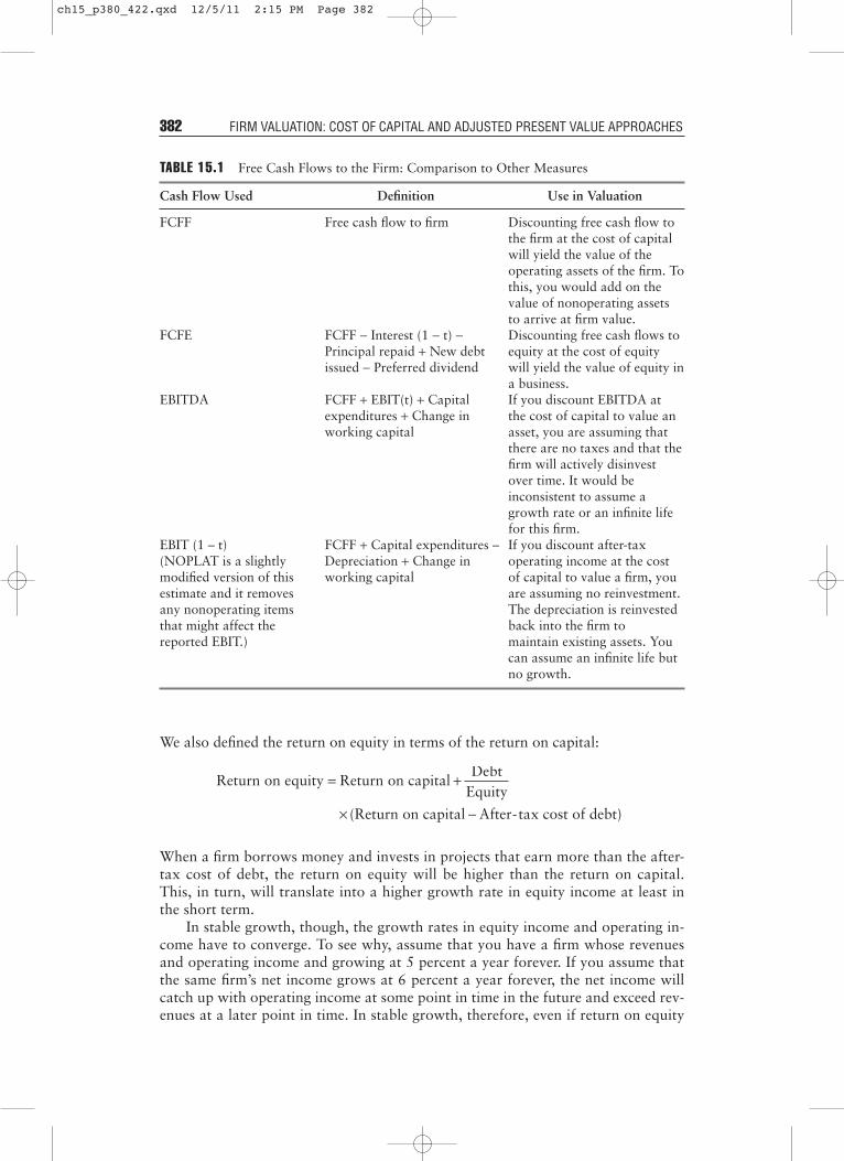
TABLE 15.1 Free Cash Flows to the Firm: Comparison to Other Measures

Cash Flow Used Definition Use in Valuation

FCFF Free cash flow to firm Discounting free cash flow to the firm at the cost of capital will yield the value of the operating assets of the firm. To this, you would add on the value of nonoperating assets to arrive at firm value.

FCFE FCFF − Interest (1 − t) − Discounting free cash flows to Principal repaid + New debt equity at the cost of equity issued − Preferred dividend will yield the value of equity in

a business.EBITDA FCFF + EBIT(t) + Capital If you discount EBITDA at

expenditures + Change in the cost of capital to value an working capital asset, you are assuming that

there are no taxes and that the firm will actively disinvest over time. It would be inconsistent to assume a growth rate or an infinite life for this firm.

EBIT (1 – t) FCFF + Capital expenditures – If you discount after-tax (NOPLAT is a slightly Depreciation + Change in operating income at the cost modified version of this working capital of capital to value a firm, you estimate and it removes are assuming no reinvestment. any nonoperating items The depreciation is reinvested that might affect the back into the firm to reported EBIT.) maintain existing assets. You

can assume an infinite life but no growth.

ch15_p380_422.qxd 12/5/11 2:15 PM Page 382

exceeds the return on capital, the expected growth will be the same in all measuresof income.1

FIRM VALUATION: THE COST OF CAPITAL APPROACH

The value of the firm is obtained by discounting the free cash flow to the firm at theweighted average cost of capital. Embedded in this value are the tax benefits of debt(in the use of the after-tax cost of debt in the cost of capital) and expected additionalrisk associated with debt (in the form of higher costs of equity and debt at higherdebt ratios). Just as with the dividend discount model and the FCFE model, the ver-sion of the model used will depend on assumptions made about future growth.

Stable Growth Firm

As with the dividend discount and FCFE models, a firm that is growing at a ratethat it can sustain in perpetuity—a stable growth rate—can be valued using a stablegrowth model.

The Model A firm with free cash flows to the firm growing at a stable growth ratecan be valued using the following equation:

where FCFF1 = Expected FCFF next yearWACC = Weighted average cost of capital

gn = Growth rate in the FCFF forever

The Caveats There are two conditions that need to be met in using this model.First, the growth rate used in the model has to be less than or equal to the growthrate in the economy—nominal growth, if the cost of capital is in nominal terms, orreal growth, if the cost of capital is a real cost of capital. Second, the characteristicsof the firm have to be consistent with assumptions of stable growth. In particular,the reinvestment rate used to estimate free cash flows to the firm should be consis-tent with the stable growth rate. The best way of enforcing this consistency is to de-rive the reinvestment rate from the stable growth rate:

If reinvestment is estimated from net capital expenditures and change in work-ing capital, the net capital expenditures should be similar to those other firms in the

Reinvestment rate in stable growthGrowth rate

Return on capital=

Value of firmFCFF

WACC g1

n

=−( )

Firm Valuation: The Cost of Capital Approach 383

1The equity reinvestment rate and firm reinvestment rate will adjust to ensure that this hap-pens. The equity reinvestment rate will be a lower number than the firm reinvestment rate instable growth for any levered firm.

ch15_p380_422.qxd 12/5/11 2:15 PM Page 383

industry (perhaps by setting the ratio of capital expenditures to depreciation at in-dustry averages) and the change in working capital should generally not be nega-tive. A negative change in working capital creates a cash inflow, and while this may,in fact, be viable for a firm in the short term, it is dangerous to assume it in perpe-tuity.2 The cost of capital should also be reflective of a stable growth firm. In partic-ular, the beta should be close to 1—the rule of thumb presented in the earlierchapters that the beta should be between 0.8 and 1.2 still holds. While stablegrowth firms tend to use more debt, this is not a prerequisite for the model, sincedebt policy is subject to managerial discretion.

Limitations Like all stable growth models, this one is sensitive to assumptionsabout the expected growth rate. This is accentuated, however, by the fact that thediscount rate used in valuation is the WACC, which is significantly lower than thecost of equity for most firms. Furthermore, the model is sensitive to assumptionsmade about capital expenditures relative to depreciation. If the inputs for reinvest-ment are not a function of expected growth the free cash flow to the firm can be in-flated (deflated) by reducing (increasing) capital expenditures relative todepreciation. If the reinvestment rate is estimated from the return on capital,changes in the return on capital can have significant effects on firm value.

ILLUSTRATION 15.1: Valuing a Firm with Stable Growth FCFF Model—Telesp (Brazil)

Telesp provides local telecommunication services to the Brazilian state of Sao Paulo. In 2010, thecompany had operating income (EBIT) of 3,544 million BRL and faced an effective tax rate of 30%. In2010, the firm reported capital expenditures of 1,659 million BRL and depreciation of 1,914 millionBRL and an increase in working capital of 1,119 million BRL. Consequently, its reinvestment in 2010can be computed as follows:

The return on capital generated by the company in 2010 was computed using the operating incomefor the year and the book value of capital invested at the end of the previous year (2009):

The expected growth rate that emerges from these inputs is:

Expected growth rate = 34.82% × 15.68% = 5.46%

384 FIRM VALUATION: COST OF CAPITAL AND ADJUSTED PRESENT VALUE APPROACHES

2Carried to its logical extreme, this will push net working capital to a very large (potentiallyinfinite) negative number.

Reinvestment =Capital expenditures − Depreciation + Change in noncash WC

EBIT(1 − t)

Value per share =1,659 − 1,914 + 1,119

3,544 (1 − .30)= 34.82%

Return on capital =EBIT2010 (1 − t)

BV of equity2009 + BV of debt2009 − Cash2009

Value per share = 3,544 (1 − .30)

10,057 + 8,042 − 12,277= 15.68%

ch15_p380_422.qxd 12/5/11 2:15 PM Page 384

While this would be too high a growth rate for stable growth in a developed market with low expectedinflation, the risk-free rate in BRL in May 2011 was 7%. In conjunction with a beta of 0.8 and an eq-uity risk premium for Brazil of 8% (composed of a mature market premium of 5% and an additionalcountry risk premium of 3% for Brazil), this yields a cost of equity of 13.40%. Incorporating a pretaxcost of debt of 9.50% and a debt ratio of 20% (based upon current market values for equity and debt)results in a cost of capital of 12.05% for Telesp:

Cost of capital = 13.40% (.80) + 9.50%(1 − .30)(.20) = 12.05%

The value for the operating assets can then be estimated as follows:

FCFF = EBIT (1 − t) + Depreciation − Capital Expenditures − Change in noncash WC = 3,544 (1 − .30) + 1,914 − 1,659 − 1,119 = 1,617 million BRL

Adding the cash and marketable securities (1,557 million BRL) and subtracting the debt (5,519 millionBRL) at the end of 2010 yields a value for the equity:

Value of equity = Value of operating assets + Cash − Debt= 25,854 + 1,557 − 5,519 = 21,892 million BRL

The company’s market capitalization in May 2011 was 21,982 million BRL, making it fairly priced.

General Version of the FCFF Model

Rather than break the free cash flow model into two-stage and three-stage modelsand risk repeating what was said in the preceding chapter, we present the generalversion of the model in this section. We follow up by examining a range of compa-nies—a traditional manufacturing firm, a firm with operating leases, and a firmwith substantial R&D investments—to illustrate the differences and similarities be-tween this approach and the FCFE approach.

The Model The value of the firm, in the most general case, can be written as thepresent value of expected free cash flows to the firm:

where FCFFt = Free cash flow to firm in year tWACC = Weighted average cost of capital

Value of firmFCFF

WACCt

tt=1

t=

=+

∞

∑( )1

Value of operating assets =Expected FCFF next year

Cost of capital − Expected growth rate

Value per share =1,617

.1205 − .0546= 25,854 million BRL

Debt to capital ratio =Debt

Debt + Market value of equity

=5,519

5,519 + 21,982= 12.05%

Firm Valuation: The Cost of Capital Approach 385

ch15_p380_422.qxd 12/5/11 2:15 PM Page 385

If the firm reaches steady state after n years and starts growing at a stable growthrate gn after that, the value of the firm can be written as:

where WACC = Cost of capital (hg: high growth; st: stable growth)

Firms Model Best Suited For Firms that either have very high leverage or are in theprocess of changing their leverage are best valued using the FCFF approach. Thecalculation of FCFE is much more difficult in these cases because of the volatilityinduced by debt payments (or new issues), and the value of equity, which is a smallslice of the total value of the firm, is more sensitive to assumptions about growthand risk. It is worth noting, though, that in theory the two approaches should yieldthe same value for the equity. Getting them to agree in practice is an entirely differ-ent challenge and we will return to examine it later in this chapter.

Value of firmFCFF

WACC

FCFF WACC g

WACC )t

hgt

t=1

t=nn+1 st n

hgn

=+

+−[ ]

+∑( )

/( )

(1 1

386 FIRM VALUATION: COST OF CAPITAL AND ADJUSTED PRESENT VALUE APPROACHES

MARKET VALUE WEIGHTS, COST OF CAPITAL, AND CIRCULAR REASONING

To value a firm, you first need to estimate a cost of capital. Every textbook iscategorical that the weights in the cost of capital calculation be market valueweights. The problem, however, is that the cost of capital is then used to esti-mate new values for debt and equity that might not match the values used inthe original calculation. One defense that can be offered for this inconsistencyis that if you bought all of the debt and equity in a publicly traded firm, youwould pay current market value and not your estimated value, and your costof capital reflects this.

For those who are bothered by this inconsistency, there is a way out. Youcould do a conventional valuation using market value weights for debt andequity, but then use the estimated values of debt and equity from the valuationto reestimate the cost of capital. This, of course, will change the values again,but you could feed the new values back and estimate cost of capital again.Each time you do this, the differences between the values you use for theweights and the values you estimate will narrow, and the values will convergesooner rather than later.

How much of a difference will it make in your ultimate value? The greaterthe difference between market value and your estimates of value, the greaterthe difference this iterative process will make. In the valuation of Tube Invest-ments, we began with a market price of Rs 92.70 per share and estimated avalue of Rs 63.36. If we substituted back this estimated value and iterated to asolution, we would arrive at an estimate of value of $70.66 per share.3

3In Microsoft Excel, it is easy to set this process up. You should first go into calculation op-tions and put a check in iteration box. You can then make the cost of capital a function ofyour estimated values for debt and equity.

ch15_p380_422.qxd 12/5/11 2:15 PM Page 386

Problems There are three problems that we see with the free cash flow to the firmmodel. The first is that the free cash flows to equity are a much more intuitive mea-sure of cash flows than cash flows to the firm. When asked to estimate cash flows,most of us look at cash flows after debt payments (free cash flows to equity), be-cause we tend to think like business owners and consider interest payments and therepayment of debt as cash outflows. Furthermore, the free cash flow to equity is areal cash flow that can be traced and analyzed in a firm. The free cash flow to thefirm is the answer to a hypothetical question: What would this firm’s cash flow be ifit had no debt (and associated payments)?

The second is that its focus on predebt cash flows can sometimes blind us toreal problems with survival. To illustrate, assume that a firm has free cash flows tothe firm of $100 million but that its large debt load makes its free cash flows to eq-uity equal to –$50 million. This firm will have to raise $50 million in new equity tosurvive, and if it cannot, all cash flows beyond this point are put in jeopardy. Usingfree cash flows to equity would have alerted you to this problem, but free cashflows to the firm are unlikely to reflect this.

The final problem is that the use of a debt ratio in the cost of capital to incor-porate the effect of leverage requires us to make implicit assumptions that mightnot be feasible or reasonable. For instance, assuming that the market value debt ra-tio is 30 percent will require a growing firm to issue large amounts of debt in futureyears to reach that ratio. In the process, the book debt ratio might reach stratos-pheric proportions and trigger covenants or other negative consequences. In fact,we count the expected tax benefits from future debt issues implicitly in the value ofequity today.

ILLUSTRATION 15.2: Valuing Target—Dealing with Operating Leases

In 2010, Target reported $5,252 million in pretax operating income on revenues of $67,390 million.While its high growth days are behind it, there is some potential for growth, and we will attempt tovalue the firm using a two stage FCFF model.

The first step in this valuation is to recognize that the financial statement numbers for Target areskewed by the failure to consider lease commitments as debt. Using the annual report for 2010, we ob-tained the lease commitments for the next five years and beyond, which we discounted at Target’s pre-tax cost of debt of 4.5% (estimated based on its S&P bond rating of A) to convert the commitments todebt:

Year Commitment Present Value @ 4.5%1 $190.00 $ 181.822 $189.00 $ 173.073 $187.00 $ 163.874 $147.00 $ 123.275 $141.00 $ 113.15

6–23 $172.22 $1,680.51Debt value of leases = $2,435.68

Note that Target reported a lump sum of $3,100 million for commitments beyond year 5, which wehave converted into annual commitments of $172.22 million a year for 18 years (a judgment call based

Firm Valuation: The Cost of Capital Approach 387

ch15_p380_422.qxd 12/5/11 2:15 PM Page 387

on the annual average commitment for years 1–5). We will adjust the stated debt and operating in-come to reflect the decision to treat lease commitments as debt:

Adjusted operating income = Stated operating income + Current year’s lease expense − Depreciation on leased asset

= $5,252 million + 200 million − (2,454/23) = $5,346 millionAdjusted debt = Stated debt + Debt value of leases

= $15,726 + $2,436 = $18,162 million

To estimate the expected growth rate, we estimated the return on capital and reinvestment rate forTarget in 2010, again staying true to the decision to capitalize leases:

Note that we computed the present value of lease commitments at the end of 2009 by going back tothe annual report for that year, extracting the lease commitments and computing the present value ofthe commitments using the pretax cost of debt at the end of 2009.

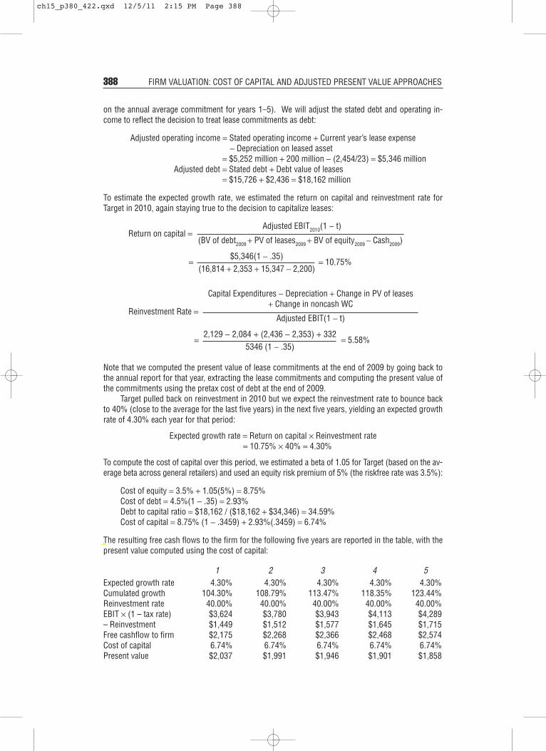
Target pulled back on reinvestment in 2010 but we expect the reinvestment rate to bounce backto 40% (close to the average for the last five years) in the next five years, yielding an expected growthrate of 4.30% each year for that period:

Expected growth rate = Return on capital × Reinvestment rate= 10.75% × 40% = 4.30%

To compute the cost of capital over this period, we estimated a beta of 1.05 for Target (based on the av-erage beta across general retailers) and used an equity risk premium of 5% (the riskfree rate was 3.5%):

Cost of equity = 3.5% + 1.05(5%) = 8.75%Cost of debt = 4.5%(1 − .35) = 2.93%Debt to capital ratio = $18,162 / ($18,162 + $34,346) = 34.59%Cost of capital = 8.75% (1 − .3459) + 2.93%(.3459) = 6.74%

The resulting free cash flows to the firm for the following five years are reported in the table, with thepresent value computed using the cost of capital:

1 2 3 4 5Expected growth rate 4.30% 4.30% 4.30% 4.30% 4.30% Cumulated growth 104.30% 108.79% 113.47% 118.35% 123.44%Reinvestment rate 40.00% 40.00% 40.00% 40.00% 40.00%EBIT × (1 – tax rate) $3,624 $3,780 $3,943 $4,113 $4,289– Reinvestment $1,449 $1,512 $1,577 $1,645 $1,715Free cashflow to firm $2,175 $2,268 $2,366 $2,468 $2,574Cost of capital 6.74% 6.74% 6.74% 6.74% 6.74%Present value $2,037 $1,991 $1,946 $1,901 $1,858

Reinvestment Rate =

Capital Expenditures − Depreciation + Change in PV of leases + Change in noncash WC

Adjusted EBIT(1 − t)

Value per share =5346 (1 − .35)

= 5.58%

Return on capital =Adjusted EBIT2010(1 − t)

(BV of debt2009 + PV of leases2009 + BV of equity2009 − Cash2009)

Value per share =$5,346(1 − .35)

(16,814 + 2,353 + 15,347 − 2,200)= 10.75%

2,129 − 2,084 + (2,436 − 2,353) + 332

388 FIRM VALUATION: COST OF CAPITAL AND ADJUSTED PRESENT VALUE APPROACHES

ch15_p380_422.qxd 12/5/11 2:15 PM Page 388

At the end of year 5, we assume that Target will be a mature firm, with a growth rate of 3% in perpe-tuity and a return on capital equal to its cost of capital. The resulting reinvestment rate and terminalvalue are estimated in the following calculations:

Return on capital in stable growth = Cost of capital in stable growth = 6.74% Reinvestment rate in stable growth = Stable growth rate/ Stable ROC

= 3%/ 6.74% = 44.54%

Adding the present value of the terminal value to the present value of the free cash flows to the firmfor the next five years, we arrive at the value of the operating assets:

Value of operating assets = PV of FCFF + PV of terminal value= $9,733 + $65,597/1.06745 = $57,086 million

Adding the cash balance ($1,712 million) and subtracting debt inclusive of the operating leases($18,162 million) yields a value of equity of $40,636 million. Dividing by the number of shares(689.13 million) results in a value per share of $58.97, about 20% higher than the prevailing marketprice of $49 in May 2011.

As a final part of the analysis, we examined the effect that treating leases as debt had on the val-uation. As the following table makes clear, staying with the current accounting treatment of operatingleases as operating expenses would have resulted in a higher return on capital, a higher cost of capi-tal, and a slightly higher value of equity per share.

Operating Expense Financial ExpenseOperating income $5,252.00 $5,346.00 Debt $16,814.00 $19,250.00ROIC 11.39% 10.75%Reinvestment rate 40% 40%Expected growth rate 4.56% 4.30%Debt to capital ratio 31.41% 34.59%Cost of capital 6.92% 6.74%Value of firm $56,731.00 $58,795.00Value of equity $41,005.00 $40,633.00Value/share $59.50 $58.97

While the value per share effect is small in the case of Target, it will be larger for firms with moresubstantial lease commitments (relative to conventional debt). A key number to track is the excessreturn (return on capital – cost of capital) earned by the firm. For Target, converting leases to debtlowers the excess return slightly from 4.47% (11.39% minus 6.92%) to 4.01% (10.75% minus6.74%), which also lowers the value per share. The greater the change in the excess returns fromthe lease adjustment, the greater will be the impact of converting leases to debt on value pershare.

Terminal value =EBIT(1 − t)6(1 − Reinvestment rate)

Cost of capital − Stable growth rate

Value per share =$4,289(1.03)(1 − .4454)

.0674 − .03= $65,597 million

Firm Valuation: The Cost of Capital Approach 389

ch15_p380_422.qxd 12/5/11 2:15 PM Page 389

ILLUSTRATION 15.3: Valuing Amgen in March 2009: The Effect of R&D Capitalization

In Illustration 9.2, we used Amgen to illustrate the effects of capitalizing R&D, using a 10-year amor-tizable life for R&D. Using data through 2008, we estimated the capital invested in R&D and the amor-tization as follows:

Amortization ThisYear R&D Expense Unamortized Portion Year

Current 3030.00 1.00 3030.00–1 3266.00 0.90 2939.40 $ 326.60–2 3366.00 0.80 2692.80 $ 336.60–3 2314.00 0.70 1619.80 $ 231.40–4 2028.00 0.60 1216.80 $ 202.80–5 1655.00 0.50 827.50 $ 165.50–6 1117.00 0.40 446.80 $ 111.70–7 864.00 0.30 259.20 $ 86.40–8 845.00 0.20 169.00 $ 84.50–9 823.00 0.10 82.30 $ 82.30

–10 663.00 0.00 0.00 $ 66.30$13283.60 $1,694.10

Using the financial statements from 2008, we computed the adjusted operating income and return oncapital at the firm.

Adjusted Operating Income = Operating income2008 + R&D expense2008 − Depreciation on R&D asset2008

= $5,594 + 3,030 − 1,694 = $ 6.930 million

Adjusted after-tax operating income = Operating income2008(1 − t) + R&D expense2008− Depreciation on R&D asset2008

= $5,594 (1 − .20) + 3,030 − 1,694 = $ 5,811 million

Note that the capitalized R&D used in the return on capital computation was based upon the R&D ex-penses through 2007 and that the adjusted after-tax earnings reflect the tax benefits of R&D expensing.

We used the restated numbers to estimate the value of the firm and equity per share. The valua-tion, where we assume ten years of high growth, is summarized in Figure 15.1:

Adjusted pretax ROIC =Adjusted operating income2008

BV of debt2007 + BV of equity2007 + Capitalized R&D2007 − Cash2007

=$6,930

$11,177 + $17,869 + $11,948 − $7,151= 20.48%

Adjusted after-tax ROIC =Adjusted after-tax operating income2008

BV of debt2007 + BV of equity2007 + Capitalized R&D2007 − Cash2007

=$5,811

$11,177 + $17,869 + $11,948 − $7,151= 17.17%

390 FIRM VALUATION: COST OF CAPITAL AND ADJUSTED PRESENT VALUE APPROACHES

ch15_p380_422.qxd 12/5/11 2:15 PM Page 390

The transition period, as in the prior chapter, exists primarily so as to allow us to adjust ourhigh growth inputs to stable growth levels. The cost of capital for instance, which is 11.23 percentfor the next five years drops in linear increments to the stable growth cost of capital of 8.23 percent;the compounded cost of capital is therefore used to discount cash flows in those years. Our estimateof value of equity per share is $67.16 a share, well above the prevailing stock price of $47.47 inMarch 2009.

An intriguing question is how the capitalization of R&D expenses affected value. To investigate,we compared the valuation fundamentals for Amgen, with conventional accounting, and with R&Dtreated as capital expenses in the following table:

Valuation Fundamentals—With and Without R&D Capitalization Conventional Capitalized R&D

After-tax ROC 20.44% 17.17%Reinvestment rate 14.47% 34.13%Growth rate 2.96% 5.86%Value per share $48.24 $67.17

We then revalued the firm, using both sets of fundamentals. As the table indicates, the valueper share would have been $48.24, if we had used conventional accounting numbers. Clearly, capi-talization matters, and the degree to which it matters will vary across firms. In general, the effectwill be negative for firms that invest large amounts in R&D, with little to show (yet) in terms ofearnings and cash flows in subsequent periods. It will be positive for firms that reinvest largeamounts in R&D and report large increases in earnings in subsequent periods. In the case ofAmgen, capitalizing R&D has a positive effect on value per share, because of its track record ofsuccessful R&D.

Firm Valuation: The Cost of Capital Approach 391

FIGURE 15.1 Valuing Amgen—March 2009

Current Cash Flow to FirmEBIT(1-t)=- Nt CpX=- Chg WC= FCFF

58111909

753828

Reinvestment Rate = 1984/5811=34.13%

Return on capital = 17.17%

Expected Growth inEBIT (1–t).3413*.1717=.05865.86%

Growth decreasesgradually to 3%

Stable Growthg = 3%; Beta = 1.10;Debt Ratio = 20%; Tax Rate = 35%;Cost of Capital = 8.23%;ROC = 10.00%; ReinvestmentRate = 3/10 = 30%

Terminal Value 10 = 5544/(.0823-.03) = 105,950

Cost of Equity12.90%

Cost of Debt(3%+1.25%)(1–.35)= 2.76%

WeightsE = 83.5% D = 16.5%

Cost of Capital (WACC) = 12.90% (0.835) + 2.76% (0.165) = 11.23%

Op. Assets 69,598+ Cash: 9,552– Debt 9,714=Equity 69,436

Value/Share $67.16

Risk-Free Rate:Riskfree rate = 3% +

Beta1.65

XRisk Premium6&

Unlevered Beta for Sectors: 1.41

Reinvestment Rate 34.13%

Return on Capital17.17%

Term Yr12184

792023765544

On March 5, 2009, Amgen was trading at $47.47/share

First 5 years

Debt ratio increases to20%Beta decreases to 1.10

D/E=21.35%

Cap Ex = Acc net Cap Ex(-401) +Acquisitions (974) + Net R&D (1336)

Year 1 2 3 4 5 6 7 8 9 10EBIT 7690

615221004052

8140651222234289

8617689423534541

9122729824914807

9657772626375089

10168813427095425

10647851827675751

11089887128086063

11829946328396624

EBIT (1-t) – Reinvestment = FCFF

Tax rateincreases to35%

11485918828326355

ch15_p380_422.qxd 12/5/11 2:15 PM Page 391

ILLUSTRATION 15.4: Valuing an Emerging Market Company with Developed Market Exposure:Gerdau Steel (Brazil) in March 2009

Gerdau Steel is a Brazilian steel company that derived about 51% of its revenues in Brazil in 2008 andthe rest in North America. We chose to value Gerdau Steel in U.S. dollars, partly because of the diffi-culties we faced in estimating risk free rates and risk premiums in Brazilian reais (R$).

To estimate the cost of capital in U.S. dollar terms, we started with the U.S. Treasury bond rate of3%. In March 2009, the equity risk premium that we were using for mature markets (like the UnitedStates) was 6% and the additional country risk premium for Brazil was 4.75%. For Gerdau Steel, we usedthe average unlevered beta of 1.01 for steel companies listed globally, using the argument that steel is acommodity that is bought and sold on a world market. Since Gerdau has a very high market debt to equityratio (138.89%), the resulting levered beta is 1.94 (with 34% being the marginal tax rate for Brazil):

Levered betaGerdau = 1.01 [1 + (1 − .34) (1.3889)] = 1.94

To reflect the fact that Gerdau Steel derives almost half its revenues in emerging markets, we esti-mated a lambda to measure exposure to Brazilian country risk, using two approaches:

1. Revenue-based approach: Dividing Gerdau’s Brazilian revenue proportion (51 percent) by the av-erage revenue proportion for a Brazilian company (72 percent) yields a lambda of 0.79.

2. Price-based approach: Regressing the weekly returns on Gerdau stock, between January 2007and January 2009, on the weekly returns on the Brazilian government dollar-denominated bondyields a lambda of 0.625:

ReturnGerdau = 0.045% + 0.6250 ReturnBrazil $ Bond

We used the latter estimate to compute a US$ cost of equity for Gerdau Steel of 17.61%:

Cost of equity for Gerdau = 3.00% + 1.94(6%) + 0.625(4.75%) = 17.61%

To estimate the cost of debt for Gerdau, we began with the interest coverage ratio for the firm, usingthe 2008 income statement:

This interest coverage ratio, in conjunction with Table 8.1 (from Chapter 8), yields a rating of A– and adefault spread of 3% (based on March 2009 spreads). Adding the default spread for Brazil (3%) at thetime, we get a pretax cost of debt of 9% for Gerdau:

Pretax cost of debt = Risk-free rate + Default spreadCountry + Default spreadCompany= 3% + 3% + 3% = 9%

Finally, incorporating Gerdau’s current market debt to capital ratio of 58.45%, we estimate a US$ costof capital of 10.79%:

Cost of capital = 17.61% (.4155) + 9% (1 − .34) (.5845) = 10.79%

We used the 2008 financial statements and exchange rates at the time of the statements to esti-mate the cashflows in R$ and then convert these cash flows to U.S. dollars.

• Base year numbers: In the 2008 financial year, Gerdau reported operating income of R$ 8,005million, after depreciation of R$ 1,896 million. During the year, acquisitions and internal in-vestments combined to create capital expenditures of R$ 6,818 million and noncash workingcapital increased by R$ 1,083 million. Gerdau earned an after-tax return on capital of 18.68%,based upon a marginal tax rate (for Brazil) of 34%, and start-of-the-year book values for

Interest coverage ratio =Operating income

Interest expenses= 8005

1620= 4.94

392 FIRM VALUATION: COST OF CAPITAL AND ADJUSTED PRESENT VALUE APPROACHES

ch15_p380_422.qxd 12/5/11 2:15 PM Page 392

equity of R$17,449 million, book value of debt of R$ 15,979 million and a cash balance of R$ 5,139 million:

• Forecasted growth and cash flows: We do not believe that either the return on capital or the rein-vestment rate is sustainable in the long term. Consequently, we use a reinvestment rate of 60%and a return on capital of 16% to estimate the expected growth rate of 9.60%, in R$, for the nextfive years.

Expected growth rate = Reinvestment rate × Return on capital = .60 × .16 = .096

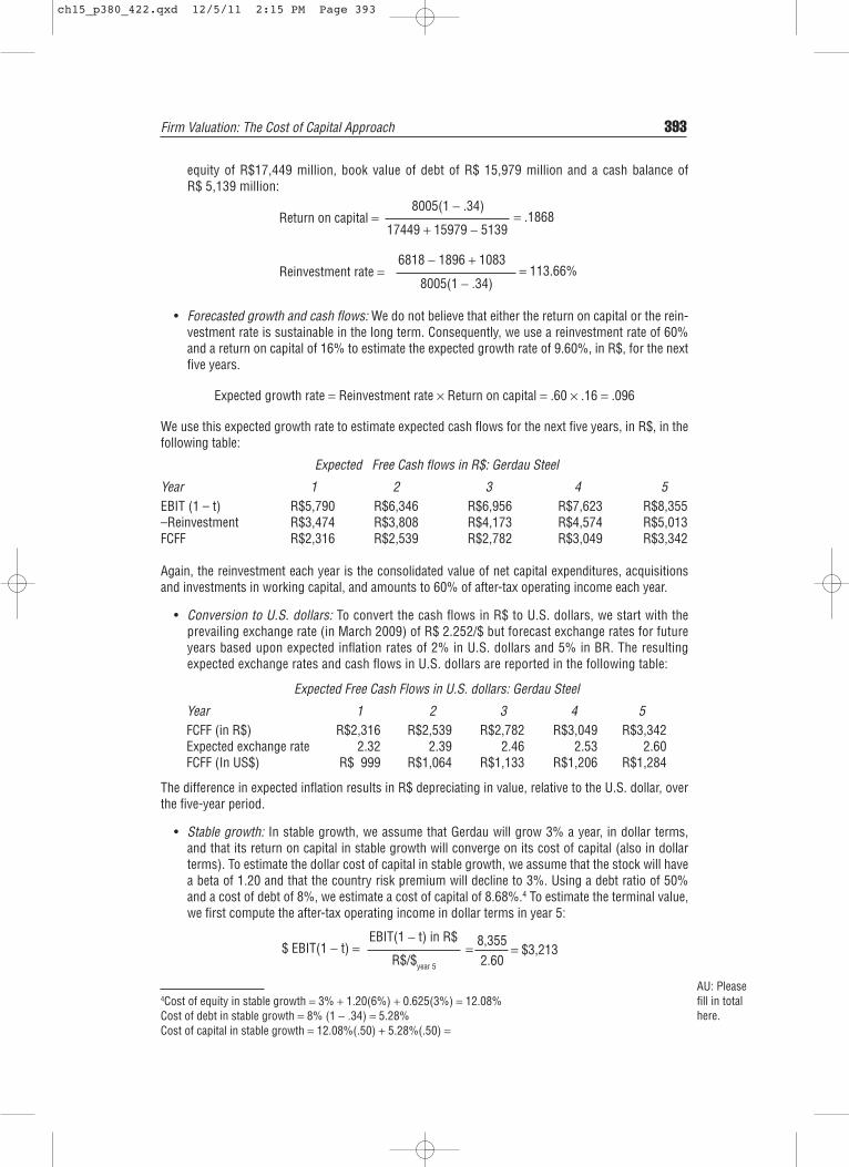
We use this expected growth rate to estimate expected cash flows for the next five years, in R$, in thefollowing table:

Expected Free Cash flows in R$: Gerdau Steel

Year 1 2 3 4 5EBIT (1 – t) R$5,790 R$6,346 R$6,956 R$7,623 R$8,355–Reinvestment R$3,474 R$3,808 R$4,173 R$4,574 R$5,013FCFF R$2,316 R$2,539 R$2,782 R$3,049 R$3,342

Again, the reinvestment each year is the consolidated value of net capital expenditures, acquisitionsand investments in working capital, and amounts to 60% of after-tax operating income each year.

• Conversion to U.S. dollars: To convert the cash flows in R$ to U.S. dollars, we start with theprevailing exchange rate (in March 2009) of R$ 2.252/$ but forecast exchange rates for futureyears based upon expected inflation rates of 2% in U.S. dollars and 5% in BR. The resultingexpected exchange rates and cash flows in U.S. dollars are reported in the following table:

Expected Free Cash Flows in U.S. dollars: Gerdau Steel

Year 1 2 3 4 5FCFF (in R$) R$2,316 R$2,539 R$2,782 R$3,049 R$3,342Expected exchange rate 2.32 2.39 2.46 2.53 2.60FCFF (In US$) R$ 999 R$1,064 R$1,133 R$1,206 R$1,284

The difference in expected inflation results in R$ depreciating in value, relative to the U.S. dollar, overthe five-year period.

• Stable growth: In stable growth, we assume that Gerdau will grow 3% a year, in dollar terms,and that its return on capital in stable growth will converge on its cost of capital (also in dollarterms). To estimate the dollar cost of capital in stable growth, we assume that the stock will havea beta of 1.20 and that the country risk premium will decline to 3%. Using a debt ratio of 50%and a cost of debt of 8%, we estimate a cost of capital of 8.68%.4 To estimate the terminal value,we first compute the after-tax operating income in dollar terms in year 5:

$ EBIT(1 − t) =EBIT(1 − t) in R$

R$/$year 5

= 8,3552.60

= $3,213

Return on capital =8005(1 − .34)

17449 + 15979 − 5139= .1868

Reinvestment rate =6818 − 1896 + 1083

8005(1 − .34)= 113.66%

Firm Valuation: The Cost of Capital Approach 393

4Cost of equity in stable growth = 3% + 1.20(6%) + 0.625(3%) = 12.08%Cost of debt in stable growth = 8% (1 − .34) = 5.28%Cost of capital in stable growth = 12.08%(.50) + 5.28%(.50) =

AU: Pleasefill in totalhere.

ch15_p380_422.qxd 12/5/11 2:15 PM Page 393

We then compute the reinvestment rate and terminal value:

• Firm and Equitoy Valuation: To complete the analysis, we first discount the expected cash flowsin US dollars at the cost of capital of 10.79%:

Expected Cash Flows and Present Value

Year 1 2 3 4 5FCFF (in U.S. $) R$ 999 R$1,064 R$1,133 R$1,206 R$1,284Terminal value 38,096Present value @ 10.79% $ 902 $ 867 $ 833 $ 800 $23,595Value of operating assets $26,996

To get to firm value, we add in dollar value of the cash holdings of the firm ($2,404 million) and subtractout the dollar value of debt ($9.788 million), with the conversion at today’s exchange rate. Since Gerdauhas consolidated holdings, we subtract out the estimated market value of the minority interest in theseholdings of $2,599 million (in dollar terms) and then divide by the number of shares outstanding(1681.12 million) to arrive at a dollar value per share of $10.12:5

Converted at the exchange rate of 2.252 R$/$, we arrive at an estimate of value of R$ 22.79/ shares,making it significantly undervalued at the price of R$9.32/share at which it was trading in March 2009.

As with the prior two valuations, it is worth exploring the effect of the choice we made to valueGerdau Steel in U.S. dollars. We could have valued Gerdau Steel in BRL by adjusting the U.S. dollarcost of capital for differential inflation:

Making a similar adjustment to the stable period cost of capital yields a BRL cost of capital of 11.88%.Finally, we adjust the stable growth rate to reflect the higher inflation rate in BRL:

⎛

⎝⎜⎞

⎠⎟.1 05.1 02

= 1.1079 = 14.05%

Stable growth rate = (1 + Stable growth rateUS$)(1 + Exp InflationBRL)

(1 + Exp InflationUS$)− 1

= 1.1079(1.05)

(1.02)= 14.05%

Cost of capital in BRL = (1 + Cost of capitalUS$) =(1 + Exp inflationBRL)

(1 + Exp inflationUS$)− 1

Value per share =26,996 + 2,403 − 9.788 − 2,599

449.82= R$10.12/share

Reinvestment rate =Stable growth rate

Stable ROC= 3%

8.68%= 34.57%

Terminal value =After-tax operating income5(1 + gstable)(1 − Reinvestment rate)

Cost of capitalstable − gstable

=$3,213(1.03)(1 − .3457)

.0868 − .03= $38,096 million

394 FIRM VALUATION: COST OF CAPITAL AND ADJUSTED PRESENT VALUE APPROACHES

5Optimally, we would have liked to value the consolidated holdings and estimate the value of the minority interests.Since we were missing much of the information necessary to do this, we applied a price-to-book ratio of 1.20 (basedon the price to book ratio of businesses that the cross holdings were in) to the book value of the minority interests.

ch15_p380_422.qxd 12/5/11 2:15 PM Page 394

The terminal value in $R can then be estimated:

The value of Gerdau Steel’s operating assets in BRL can then be computed by discounting the BRLcash flows back at the BRL cost of capital:

Year 1 2 3 4 5FCFF (in R$) R$ 2,316 R$2,539 R$2,782 R$3,049 R$ 3,342TV R$96,230PV R$ 2,031 R$1,952 R$1,875 R$1,802 R$51,601Value of operating

assets = R$59,261

Converting the value into US$ at the prevailing exchange rate of 2.252 yields a dollar value for the op-erating assets of $26,315 million, very close to our dollar-based estimate of $26,996 million.

Terminal value =After-tax operating income5(1 + gstable)(1 − Reinvestement rate)

(Cost of capitalstable − gstable)

=$R8,355(1.0603)(1 − .3457)

(.1189 − .0603)= R$96,230 million

Firm Valuation: The Cost of Capital Approach 395

fcffginzu.xls: This spreadsheet allows you to estimate the value of a firm using theFCFF approach.

NET DEBT VERSUS GROSS DEBT

In valuing the companies in this chapter, we used total debt outstanding (grossdebt) rather than net debt where cash was netted out against debt. What is thedifference between the two approaches, and will the valuations from the twoapproaches agree?

A comparison of gross and net debt valuations reveals the differences inthe way we approach the calculation of key inputs to the valuation, summa-rized as follows:

Gross Debt Net DebtLevered beta Unlevered beta is levered Unlevered beta is levered

using gross debt to market using net debt to market equity ratio. equity ratio.

Cost of capital Debt-to-capital ratio used Debt-to-capital ratio used is is based on gross debt. based on net debt.

Treatment of Cash is added to value Cash is not added back to cash and debt of operating assets and operating assets and net debt

gross debt is subtracted is subtracted to get to equityto get to equity value. value.

While working with net debt in valuation is not difficult to do, the moreinteresting question is whether the value that emerges will be the same as thevalue that would have been estimated using gross debt. In general the answer

(continued)

ch15_p380_422.qxd 12/5/11 2:15 PM Page 395

Will Equity Value Be the Same under Firm and Equity Valuation?

This model, unlike the dividend discount model or the FCFE model, values the firmrather than equity. The value of equity, however, can be extracted from the value ofthe firm by subtracting the market value of outstanding debt. Since this model canbe viewed as an alternative way of valuing equity, two questions arise: Why valuethe firm rather than equity? Will the values for equity obtained from the firm valu-ation approach be consistent with the values obtained from the equity valuationapproaches described in the previous chapter?

The advantage of using the firm valuation approach is that cash flows relatingto debt do not have to be considered explicitly since the FCFF is a predebt cashflow, while they have to be taken into account in estimating FCFE. In cases wherethe leverage is expected to change significantly over time, this is a significant savings,since estimating new debt issues and debt repayments when leverage is changingcan become increasingly messy the further into the future you go. The firm valua-tion approach does, however, require information about debt ratios and interestrates to estimate the weighted average cost of capital.

The value for equity obtained from the firm valuation and equity valuation ap-proaches will be the same if you make consistent assumptions about financial lever-age. Getting them to converge in practice is much more difficult. Let us begin with

396 FIRM VALUATION: COST OF CAPITAL AND ADJUSTED PRESENT VALUE APPROACHES

is no, and the reason usually lies in the cost of debt used in the net debt valua-tion. Intuitively, what you are doing when you use net debt is break the firminto two parts—a cash business, which is funded 100 percent with risklessdebt, and an operating business funded partly with risky debt. Carrying thisto its logical conclusion, the cost of debt you would have for the operatingbusiness would be significantly higher than the firm’s current cost of debt.This is because the current lenders to the firm will factor in the firm’s cashholdings when setting the cost of debt.

To illustrate, assume that you have a firm with an overall value of $1 bil-lion—$200 million in cash and $800 million in operating assets—with $400 mil-lion in debt and $600 million in equity. The firm’s cost of debt is 7 percent, a 2percent default spread over the risk-free rate of 5 percent; note that this cost ofdebt is set based on the firm’s substantial cash holdings. If you net debt againstcash, the firm would have $200 million in net debt and $600 million in equity. Ifyou use the 7 percent cost of debt to value the firm now, you will overstate itsvalue. Instead, the cost of debt you should use in the valuation is 9 percent:

Cost of debt on net debt = (Pretax cost of debtgross debt × Gross debt − Risk ratenet debt × Cash)/(Gross debt − Cash)

= (.07 × 400 − .05 × 200)/(400 − 200) = .09In general, we would recommend using gross debt rather than net debt

for two other reasons. First, the net debt can be a negative number if cash ex-ceeds the gross debt. If this occurs, you should set the net debt to zero andconsider the excess cash just as you would cash in a gross debt valuation. Sec-ond, maintaining a stable net debt ratio in a growing firm will require thatcash balances increase as the firm value increases.

ch15_p380_422.qxd 12/5/11 2:15 PM Page 396

the simplest case—a no-growth, perpetual firm. Assume that the firm has $166.67million in earnings before interest and taxes and a tax rate of 40 percent. Assumethat the firm has equity with a market value of $600 million, with a cost of equityof 13.87 percent, and debt of $400 million, with a pretax cost of debt of 7 percent.The firm’s cost of capital can be estimated as follows:

Cost of capital = 13.87%(700/1,000) + 7%(1 − .4)(300/1,000) = 10%

Value of the firm = Earnings before interest and taxes(1 − t)/Cost of capital= 166.67(1 − .4)/.10 = $1,000

Note that the firm has no reinvestment and no growth. We can value equity in thisfirm by subtracting the value of debt:

Value of equity = Value of firm − Value of debt = $1,000 − $400 = $600 million

Now let us value the equity directly by estimating the net income:

Net income = (EBIT − Pretax cost of debt × Debt)(1 − t)= (166.67 − .07 × 400)(1 − .4) = $83.202 million

The value of equity can be obtained by discounting this net income at the cost ofequity:

Value of equity = Net income/Cost of equity = 83.202/.1387 = $600 million

Even this simple example works because of the following three assumptions madeimplicitly or explicitly during the valuation:

1. The values for debt and equity used to compute the cost of capital were equalto the values obtained in the valuation. Notwithstanding the circularity in rea-soning—you need the cost of capital to obtain the values in the first place—itindicates that a cost of capital based on market value weights will not yield thesame value for equity as an equity valuation model if the firm is not fairlypriced in the first place.

2. There are no extraordinary or nonoperating items that affect net income butnot operating income. Thus, to get from operating to net income all we do issubtract interest expenses and taxes.

3. The interest expenses are equal to the pretax cost of debt multiplied by themarket value of debt. If a firm has old debt on its books, with interest expensesthat are different from this value, the two approaches will diverge.

If there is expected growth, the potential for inconsistency multiplies. You have toensure that you borrow enough money to fund new investments to keep your debtratio at a level consistent with what you are assuming when you compute the costof capital.

Firm Valuation: The Cost of Capital Approach 397

fcffvsfcfe.xls: This spreadsheet allows you to compare the equity values obtainedusing FCFF and FCFE models.

ch15_p380_422.qxd 12/5/11 2:15 PM Page 397

FIRM VALUATION: THE ADJUSTED PRESENT VALUE APPROACH

The adjusted present value (APV) approach begins with the value of the firm with-out debt. As debt is added to the firm, the net effect on value is examined by con-sidering both the benefits and the costs of borrowing. To do this, it is assumed thatthe primary benefit of borrowing is a tax benefit, and that the most significant costof borrowing is the added risk of bankruptcy.

Mechanics of APV Valuation

We estimate the value of the firm in three steps:

1. Estimate the value of the firm with no leverage.2. Consider the present value of the interest tax savings generated by borrowing a

given amount of money.3. Evaluate the effect of borrowing the amount on the probability that the firm

will go bankrupt, and the expected cost of bankruptcy.

Value of Unlevered Firm The first step in this approach is the estimation of the valueof the unlevered firm. This can be accomplished by valuing the firm as if it had nodebt (i.e., by discounting the expected free cash flow to the firm at the unlevered costof equity). In the special case where cash flows grow at a constant rate in perpetuity,

Value of unlevered firm = E(FCFF1)/(ρu − g)

where FCFF1 is the expected after-tax operating cash flow to the firm, ρu is theunlevered cost of equity, and g is the expected growth rate. In the more generalcase, you can value the firm using any set of growth assumptions you believe arereasonable for the firm.

The inputs needed for this valuation are the expected cash flows, growth rates,and the unlevered cost of equity. To estimate the unlevered cost of equity, we candraw on our earlier analysis and compute the unlevered beta of the firm:

βunlevered = βcurrent/[1 + (1 − t)D/E]

where βunlevered = Unlevered beta of the firmβcurrent = Current equity beta of the firm

t = Tax rate for the firmD/E = Current debt/equity ratio

This unlevered beta can then be used to arrive at the unlevered cost of equity.

Expected Tax Benefit from Borrowing The second step in this approach is the cal-culation of the expected tax benefit from a given level of debt. This tax benefit is afunction of the tax rate and interest payments of the firm and is discounted at thecost of debt to reflect the riskiness of this cash flow. If the tax savings are viewed asa perpetuity,

Value of tax benefits = (Tax rate × Cost of debt × Debt)/Cost of debt= Tax rate × Debt = tcD

398 FIRM VALUATION: COST OF CAPITAL AND ADJUSTED PRESENT VALUE APPROACHES

ch15_p380_422.qxd 12/5/11 2:15 PM Page 398

The tax rate used here is the firm’s marginal tax rate, and it is assumed to stay con-stant over time. If we anticipate the tax rate changing over time, we can still com-pute the present value of tax benefits over time, but we cannot use the perpetualgrowth equation cited earlier. In addition, you would have to modify this equationif the current interest expenses do not reflect the current cost of debt.

Estimating Expected Bankruptcy Costs and Net Effect The third step is to evaluatethe effect of the given level of debt on the default risk of the firm and on expectedbankruptcy costs. In theory, at least, this requires the estimation of the probabilityof default with the additional debt and the direct and indirect cost of bankruptcy. Ifπa is the probability of default after the additional debt and BC is the present valueof the bankruptcy cost, the present value (PV) of expected bankruptcy cost can beestimated:

PV of expected bankruptcy cost = Probability of bankruptcy × PV of bankruptcy cost= πaBC

This step of the adjusted present value approach poses the most significant estima-tion problems, since neither the probability of bankruptcy nor the bankruptcy costcan be estimated directly.

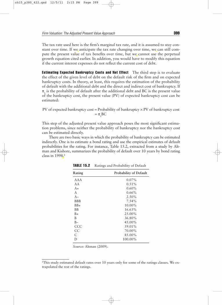
There are two basic ways in which the probability of bankruptcy can be estimatedindirectly. One is to estimate a bond rating and use the empirical estimates of defaultprobabilities for the rating. For instance, Table 15.2, extracted from a study by Alt-man and Kishore, summarizes the probability of default over 10 years by bond ratingclass in 1998.6

Firm Valuation: The Adjusted Present Value Approach 399

6This study estimated default rates over 10 years only for some of the ratings classes. We ex-trapolated the rest of the ratings.

TABLE 15.2 Ratings and Probability of Default

Rating Probability of Default

AAA 0.07%AA 0.51%A+ 0.60%A 0.66%A– 2.50%BBB 7.54%BB+ 10.00%BB 16.63%B+ 25.00%B 36.80%B– 45.00%CCC 59.01%CC 70.00%C 85.00%D 100.00%

Source: Altman (2009).

ch15_p380_422.qxd 12/5/11 2:15 PM Page 399

The other way is to use a statistical approach such as a probit to estimate theprobability of default, based on the firm’s observable characteristics, at each levelof debt.

The bankruptcy cost can be estimated, albeit with considerable error, fromstudies that have looked at the magnitude of this cost in actual bankruptcies. Re-search that has looked at the direct cost of bankruptcy concludes that they aresmall7 relative to firm value. The indirect costs of bankruptcy can be substantial,but the costs vary widely across firms. Shapiro and Titman speculate that the indi-rect costs could be as large as 25 to 30 percent of firm value but provide no directevidence of the costs.

ILLUSTRATION 15.5: Valuing a Company Using APV: The Leveraged Acquisition of J. Crew

J. Crew is a U.S. retailer that sells clothes made under its brand name through its own stores and on-line. In 2010, the firm was acquired in a leveraged deal by Mickey Drexler, its CEO, and two private eq-uity firms—TPG and Leonard Green—for $ 2.7 billion, with about $1.85 billion coming from debt(with a rating of BB and a pretax cost of debt of 7%).

To assess the value of the deal, using the APV approach, we first valued the firm as an all-equityfunded (unlevered) firm. To estimate the value, we first computed a cost of equity using an unleveredbeta of 1.00 for specialty retailers, in conjunction with a riskfree rate of 3.5% and mature market pre-mium of 5%:

Unlevered cost of equity = 3.5% + 1.00(5%) = 8.5%

J. Crew generated $230 million in operating income on revenues of $1,722 million in 2010. We as-sumed a 35% tax rate and a growth rate of 3.5% in perpetuity, with a return on capital of 14%., re-sulting in the following:

Reinvestment rate in stable growth = g/ ROC = 3.5%/14% = 25%

FCFF in most recent year = EBIT (1 − t) (1 − Reinvestment rate)= 230 (1 − .35) (1 − .25) = $112.125 million

To estimate the tax benefits from debt, we assumed that a debt schedule, where the dollar debtwould be repaid in equal annual increments to a debt level of $500 million in year 10 and beyond.Using the 35 percent tax rate and the pretax cost of debt, we compute the interest expenses and taxbenefits each year, and discount these benefits back to today, using the pretax cost of debt as thediscount rate.

400 FIRM VALUATION: COST OF CAPITAL AND ADJUSTED PRESENT VALUE APPROACHES

7In Warner’s study of railroad bankruptcies, the direct cost of bankruptcy seems to be about5 percent.

Unlevered firm value =Expected FCFF next year

Unlevered cost of equity − Stable growth rate− 1

=$112.125(1.035)

.085 − .035= $2,321 million

ch15_p380_422.qxd 12/5/11 2:15 PM Page 400

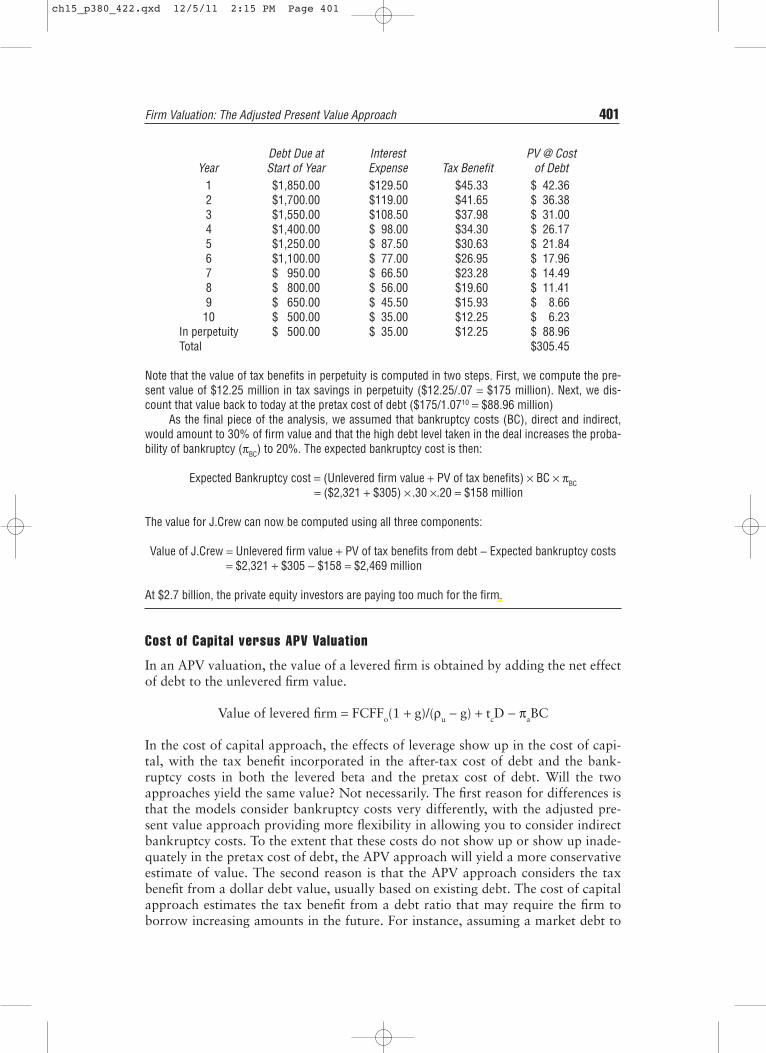
Debt Due at Interest PV @ Cost Year Start of Year Expense Tax Benefit of Debt

1 $1,850.00 $129.50 $45.33 $ 42.362 $1,700.00 $119.00 $41.65 $ 36.383 $1,550.00 $108.50 $37.98 $ 31.004 $1,400.00 $ 98.00 $34.30 $ 26.175 $1,250.00 $ 87.50 $30.63 $ 21.84 6 $1,100.00 $ 77.00 $26.95 $ 17.967 $ 950.00 $ 66.50 $23.28 $ 14.498 $ 800.00 $ 56.00 $19.60 $ 11.419 $ 650.00 $ 45.50 $15.93 $ 8.6610 $ 500.00 $ 35.00 $12.25 $ 6.23

In perpetuity $ 500.00 $ 35.00 $12.25 $ 88.96Total $305.45

Note that the value of tax benefits in perpetuity is computed in two steps. First, we compute the pre-sent value of $12.25 million in tax savings in perpetuity ($12.25/.07 = $175 million). Next, we dis-count that value back to today at the pretax cost of debt ($175/1.0710 = $88.96 million)

As the final piece of the analysis, we assumed that bankruptcy costs (BC), direct and indirect,would amount to 30% of firm value and that the high debt level taken in the deal increases the proba-bility of bankruptcy (πBC) to 20%. The expected bankruptcy cost is then:

Expected Bankruptcy cost = (Unlevered firm value + PV of tax benefits) × BC × πBC= ($2,321 + $305) × .30 ×.20 = $158 million

The value for J.Crew can now be computed using all three components:

Value of J.Crew = Unlevered firm value + PV of tax benefits from debt − Expected bankruptcy costs= $2,321 + $305 − $158 = $2,469 million

At $2.7 billion, the private equity investors are paying too much for the firm.

Cost of Capital versus APV Valuation

In an APV valuation, the value of a levered firm is obtained by adding the net effectof debt to the unlevered firm value.

Value of levered firm = FCFFo(1 + g)/(ρu − g) + tcD − πaBC

In the cost of capital approach, the effects of leverage show up in the cost of capi-tal, with the tax benefit incorporated in the after-tax cost of debt and the bank-ruptcy costs in both the levered beta and the pretax cost of debt. Will the twoapproaches yield the same value? Not necessarily. The first reason for differences isthat the models consider bankruptcy costs very differently, with the adjusted pre-sent value approach providing more flexibility in allowing you to consider indirectbankruptcy costs. To the extent that these costs do not show up or show up inade-quately in the pretax cost of debt, the APV approach will yield a more conservativeestimate of value. The second reason is that the APV approach considers the taxbenefit from a dollar debt value, usually based on existing debt. The cost of capitalapproach estimates the tax benefit from a debt ratio that may require the firm toborrow increasing amounts in the future. For instance, assuming a market debt to

Firm Valuation: The Adjusted Present Value Approach 401

ch15_p380_422.qxd 12/5/11 2:15 PM Page 401

capital ratio of 30 percent in perpetuity for a growing firm will require it to borrowmore in the future, and the tax benefit from expected future borrowings is incorpo-rated into value today. Generally speaking, the cost-of-capital approach is a morepractical choice when valuing ongoing firms that are not going through contortionson financial leverage; it is easier to work with a debt ratio than with dollar-debt lev-els. The APV approach is more useful for transactions that are funded dispropor-tionately with debt and where debt repayment schedules are negotiated or known;this is why it has acquired a footing in leveraged-buyout circles.

EFFECT OF LEVERAGE ON FIRM VALUE

Both the cost of capital approach and the APV approach make the value of a firm afunction of its leverage. It follows directly, then, that there is some mix of debt andequity at which firm value is maximized. The rest of this chapter considers howbest to make this link.

Cost of Capital and Optimal Leverage

In order to understand the relationship between the cost of capital and optimal cap-ital structure, we rely on the relationship between firm value and the cost of capital.The earlier section noted that the value of the entire firm can be estimated by dis-counting the expected cash flows to the firm at the firm’s cost of capital.

The firm value can then be written as follows:

and is a function of the firm’s cash flows and its cost of capital. If we assume that thecash flows to the firm are unaffected by the choice of financing mix, and the cost ofcapital is reduced as a consequence of changing the financing mix, the value of thefirm will increase. If the objective in choosing the financing mix for the firm is themaximization of firm value, we can accomplish it, in this case, by minimizing the costof capital. In the more general case where the cash flows to the firm are a function ofthe debt-equity mix, the optimal financing mix is the mix that maximizes firm value.8

Value of firmCF to firm

WACCtt

t=1

t=n

=+∑

( )1

402 FIRM VALUATION: COST OF CAPITAL AND ADJUSTED PRESENT VALUE APPROACHES

APV WITHOUT BANKRUPTCY COSTS

There are many who believe that adjusted present value is a more flexible wayof approaching valuation than traditional discounted cash flow models. Thismay be true in a generic sense, but APV valuation in practice has significantflaws. The first and most important is that most practitioners who use the ad-justed present value model ignore expected bankruptcy costs. Adding the taxbenefits to unlevered firm value to get to levered firm value makes debt seemlike an unmixed blessing. Firm value will be overstated, especially at very highdebt ratios, where the cost of bankruptcy is clearly not zero.

8In other words, the value of the firm might not be maximized at the point that cost of capi-tal is minimized, if firm cash flows are much lower at that level.

ch15_p380_422.qxd 12/5/11 2:15 PM Page 402

ILLUSTRATION 15.6: WACC, Firm Value, and Leverage

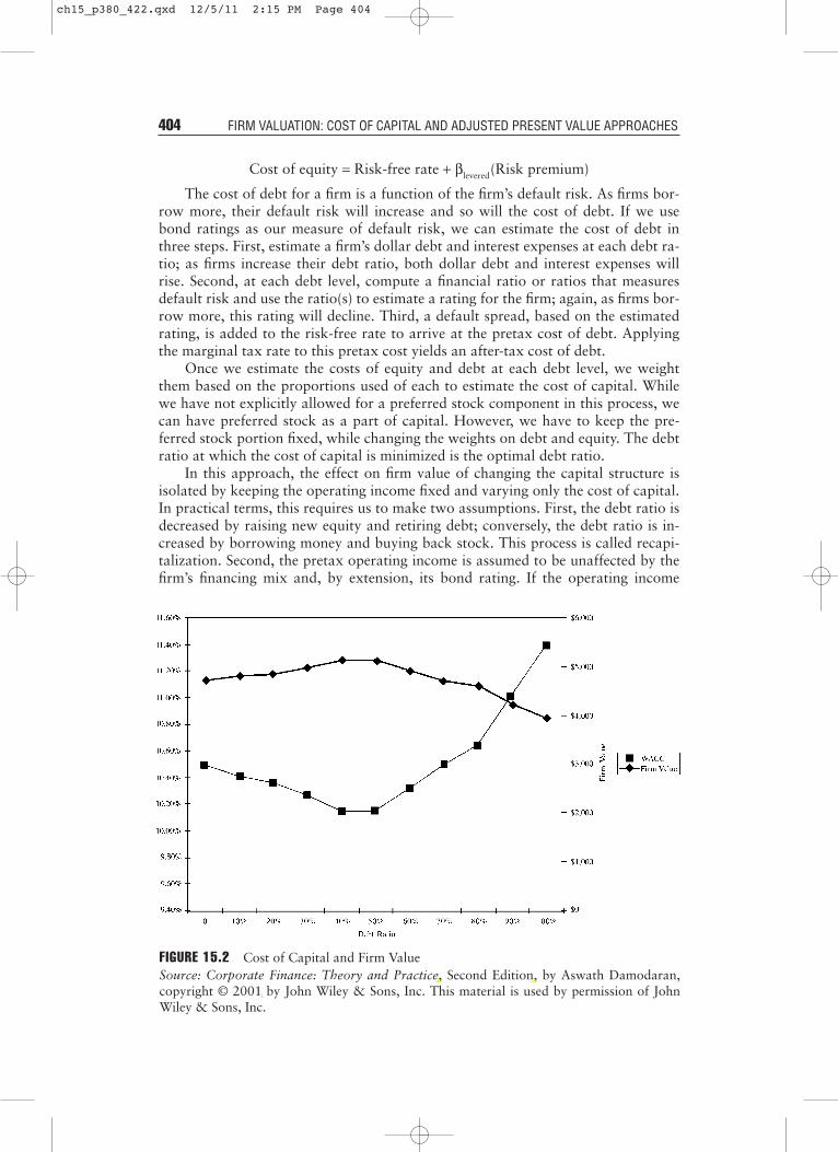
Assume that you are given the costs of equity and debt at different debt levels for Strunks Inc., a lead-ing manufacturer of chocolates and other candies, and that the cash flows to this firm are currently$200 million. Strunks is in a relatively stable market, and these cash flows are expected to grow at 6%forever and to be unaffected by the debt ratio of the firm. The cost of capital schedule is provided inthe following table, along with the value of the firm at each level of debt.

D/(D + E) Cost of Equity Cost of Debt WACC Firm Value0% 10.50% 4.80% 10.50% $4,711

10% 11.00% 5.10% 10.41% $4,80720% 11.60% 5.40% 10.36% $4,86230% 12.30% 5.52% 10.27% $4,97040% 13.10% 5.70% 10.14% $5,12150% 14.00% 6.30% 10.15% $5,10860% 15.00% 7.20% 10.32% $4,90770% 16.10% 8.10% 10.50% $4,71180% 17.20% 9.00% 10.64% $4,56990% 18.40% 10.20% 11.02% $4,223

100% 19.70% 11.40% 11.40% $3,926

Note that:

Value of firm = Cash flows to firm × (1 + g)/(Cost of capital − g) = $200 × 1.06/(Cost of capital − .06)

The value of the firm increases as the cost of capital decreases, and decreases as the cost ofcapital increases. This is illustrated in Figure 15.2. While this illustration makes the choice of an opti-mal financing mix seem easy, it obscures problems that may arise in its practice. First, we typically donot have the benefit of having the entire schedule of costs of financing prior to an analysis. In mostcases, the only level of debt at which we have information on the cost of debt and equity financing isthe current level. Second, the analysis assumes implicitly that the level of operating income of thefirm is unaffected by the financing mix of the firm and, consequently, by the default risk (or bond rat-ing) for the firm. While this may be reasonable in some cases, it might not be in others. Firms thatborrow too much might find that there are indirect bankruptcy costs that affect revenues and operat-ing income.

Steps in Cost of Capital Approach We need three basic inputs to compute the costof capital—the cost of equity, the after-tax cost of debt, and the weights on debtand equity. The costs of equity and debt change as the debt ratio changes, and theprimary challenge of this approach is in estimating each of these inputs.

Let us begin with the cost of equity. We argued that the beta of equity willchange as the debt ratio changes. In fact, we estimated the levered beta as a func-tion of the market debt to equity ratio of a firm, the unlevered beta and the firm’smarginal tax rate:

βlevered = βunlevered[1 + (1 − t)Debt/Equity]

Thus, if we can estimate the unlevered beta for a firm, we can use it to estimate thelevered beta of the firm at every debt ratio. This levered beta can then be used tocompute the cost of equity at each debt ratio.

Effect of Leverage on Firm Value 403

ch15_p380_422.qxd 12/5/11 2:15 PM Page 403

Cost of equity = Risk-free rate + βlevered(Risk premium)

The cost of debt for a firm is a function of the firm’s default risk. As firms bor-row more, their default risk will increase and so will the cost of debt. If we usebond ratings as our measure of default risk, we can estimate the cost of debt inthree steps. First, estimate a firm’s dollar debt and interest expenses at each debt ra-tio; as firms increase their debt ratio, both dollar debt and interest expenses willrise. Second, at each debt level, compute a financial ratio or ratios that measuresdefault risk and use the ratio(s) to estimate a rating for the firm; again, as firms bor-row more, this rating will decline. Third, a default spread, based on the estimatedrating, is added to the risk-free rate to arrive at the pretax cost of debt. Applyingthe marginal tax rate to this pretax cost yields an after-tax cost of debt.

Once we estimate the costs of equity and debt at each debt level, we weightthem based on the proportions used of each to estimate the cost of capital. Whilewe have not explicitly allowed for a preferred stock component in this process, wecan have preferred stock as a part of capital. However, we have to keep the pre-ferred stock portion fixed, while changing the weights on debt and equity. The debtratio at which the cost of capital is minimized is the optimal debt ratio.

In this approach, the effect on firm value of changing the capital structure isisolated by keeping the operating income fixed and varying only the cost of capital.In practical terms, this requires us to make two assumptions. First, the debt ratio isdecreased by raising new equity and retiring debt; conversely, the debt ratio is in-creased by borrowing money and buying back stock. This process is called recapi-talization. Second, the pretax operating income is assumed to be unaffected by thefirm’s financing mix and, by extension, its bond rating. If the operating income

404 FIRM VALUATION: COST OF CAPITAL AND ADJUSTED PRESENT VALUE APPROACHES

FIGURE 15.2 Cost of Capital and Firm ValueSource: Corporate Finance: Theory and Practice, Second Edition, by Aswath Damodaran,copyright © 2001 by John Wiley & Sons, Inc. This material is used by permission of JohnWiley & Sons, Inc.

ch15_p380_422.qxd 12/5/11 2:15 PM Page 404

changes with a firm’s default risk, the basic analysis will not change, but minimiz-ing the cost of capital may not be the optimal course of action, since the value ofthe firm is determined by both the cash flows and the cost of capital. The value ofthe firm will have to be computed at each debt level and the optimal debt ratio willbe that which maximizes firm value.

ILLUSTRATION 15.7: Analyzing the Capital Structure for Disney: May 2009

The cost of capital approach can be used to find the optimal capital structure for a firm, as we will forDisney in May 2009. Disney had $14,962 million in interest-bearing debt on its books and adding thepresent value of operating lease commitments of $1,720 million to this value, we arrive at a totalmarket value for the debt of $16,682 million. The market value of equity at the same time was$45,193 million; the market price per share was $24.34, and there were 1856.752 million sharesoutstanding. Proportionally, 26.96% of the overall financing mix was debt, and the remaining73.04% was equity.

The unlevered beta for Disney’s stock in May 2009, estimated by breaking it down into its con-stituent businesses and weighting the unlevered betas for each business, was 0.7333.

Revenues in Estimated Firm Value Unlevered Business 2008 EV/Sales Value Proportion BetaMedia networks $16,116 2.13 $34,328 58.92% 0.7056Parks and resorts $11,504 1.51 $17,408 29.88% 0.5849Studio entertainment $ 7,348 0.78 $ 5,755 9.88% 1.3027Consumer products $ 2,875 0.27 $ 768 1.32% 1.0690Disney operations $37,843 $58,259 100.00% 0.7333

The Treasury bond rate at that time was 3.5%. Using an estimated equity risk premium of 6%, weestimated the cost of equity for Disney to be 8.91%:

Levered beta = 0.7333 (1 + (1 − .38)(16,682/45,193)) = 0.9011Cost of equity = Risk-free rate + Beta × (Market premium) = 3.5% + 0.9011(6%) = 8.91%

Disney’s bond rating in May 2009 was A, and based on this rating, the estimated pretax cost of debtfor Disney is 6%. Using a marginal tax rate of 38%, we estimate the after-tax cost of debt for Disneyto be 3.72%.

After-tax cost of debt = Pretax interest rate (1 − Tax rate)= 6.00% (1 − 0.38) = 3.72%

The cost of capital was calculated using these costs and the weights based on market value:

DISNEY’S COST OF EQUITY AND LEVERAGE

The cost of equity for Disney at different debt ratios can be computed using the unlevered beta of thefirm, and the debt equity ratio at each level of debt. We use the levered betas that emerge to estimate

Cost of capital = Cost of equityEquity

Debt + Equity+ Cost of debt (1 − t)

Debt

Debt + Equity

= 8.91%45.193

16,682 + 45,193+ 3.72%

16,682

16,682 + 45,193= 7.51%

Effect of Leverage on Firm Value 405

ch15_p380_422.qxd 12/5/11 2:15 PM Page 405

the cost of equity. The first step in this process is to compute the levered beta at each debt ratio, us-ing this unlevered beta and Disney’s marginal tax rate of 38%:

Levered Beta = 0.7033 [1 + (1 − .38) (Debt/Equity)]

We continued to use the Treasury bond rate of 3.5% and the market premium of 6% to compute thecost of equity at each level of debt. If we keep the tax rate constant at 38%, we obtain the levered be-tas for Disney in the following table:

Levered Beta and Cost of Equity: Disney

Debt to Capital Ratio D/E Ratio Levered Beta Cost of Equity0% 0.00% 0.7333 7.90%

10% 11.11% 0.7838 8.20%20% 25.00% 0.8470 8.58%30% 42.86% 0.9281 9.07%40% 66.67% 1.0364 9.72%50% 100.00% 1.1879 10.63%60% 150.00% 1.4153 11.99%70% 233.33% 1.7941 14.26%80% 400.00% 2.5519 18.81%90% 900.00% 4.8251 32.45%

In calculating the levered beta in this table, we assumed that all market risk is borne by the equity in-vestors; this may be unrealistic especially at higher levels of debt and that the firm will be able to getthe full tax benefits of interest expenses even at very high debt ratios. We will also consider an alter-native estimate of levered betas that apportions some of the market risk to the debt:

βlevered = βu[1 + (1 − t)D/E] − βdebt (1 − t)D/E

The beta of debt can be based on the rating of the bond, estimated by regressing past returns onbonds in each rating class against returns on a market index or backed out of the default spread. Thelevered betas estimated using this approach will generally be lower than those estimated with theconventional model.9 We will also examine whether the full benefits of interest expenses will accrue athigher debt ratios.

DISNEY’S COST OF DEBT AND LEVERAGE

There are several financial ratios that are correlated with bond ratings, and we face two choices. One isto build a model that includes several financial ratios to estimate the synthetic ratings at each debt ra-tio. In addition to being more labor and data intensive, the approach will make the ratings process lesstransparent and more difficult to decipher. The other is to stick with the simplistic approach that we de-veloped in Chapter 8, of linking the rating to the interest coverage ratio, with the ratio defined as:

Interest coverage ratio =Earnings before interest and taxes

Interest expenses

406 FIRM VALUATION: COST OF CAPITAL AND ADJUSTED PRESENT VALUE APPROACHES

9Consider, for instance, a debt ratio of 40 percent. At this level the firm’s debt will take on some of the characteris-tics of equity. Assume that the beta of debt at a 40 percent debt ratio is 0.10. The equity beta at that debt ratio canbe computed as follows:

Levered Beta = 0.7333 (1 + (1 − 0.38)(40/60) − 0.10 (1 − 0.373) (40/60) = 0.99

In the unadjusted approach, the levered beta would have been 1.0364.

ch15_p380_422.qxd 12/5/11 2:15 PM Page 406

We will stick with the simpler approach for three reasons. First, we are not aiming for precision in thecost of debt, but an approximation. Given that the more complex approaches also give approxima-tions, we will tilt in favor of transparency. Second, there is significant correlation not only between theinterest coverage ratio and bond ratings but also between the interest coverage ratio and other ratiosused in analysis, such as the debt coverage ratio and the funds flow ratios. In other words, we may beadding little by adding other ratios that are correlated with interest coverage ratios, includingEBITDA/Fixed Charges, to the mix. Third, the interest coverage ratio changes as a firm changes itsfinancing mix and decreases as the debt ratio increases, a key requirement since we need the cost ofdebt to change as the debt ratio changes.

To make our estimates of the synthetic rating, we will use the lookup table that we introducedin Chapter 8, for large market capitalization firms (since Disney’s market capitalization is greater than$ 5 billion) and use the default spreads from early 2009 to estimate the pre-tax cost of debt. The fol-lowing table reproduces those numbers:

Interest Coverage Ratios, Ratings and Default Spreads—Early 2009

Interest Coverage Ratio Rating Typical Default Spread>8.5 AAA 1.25%

6.5–8.5 AA 1.75%5.5–6.5 A+ 2.25%4.25–5.5 A 2.50%3–4.25 A– 3.00%2.5–3.0 BBB 3.50%2.25–2.5 BB+ 4.25%2.0–2.25 BB 5.00%1.75–2.0 B+ 6.00%1.5–1.75 B 7.25%1.25–1.5 B– 8.50%0.8–1.25 CCC 10.00%0.65–0.8 CC 12.00%0.2–0.65 C 15.00%

<0.2 D 20.00%Source: Capital IQ & Bondsonline.com

Using this table as a guideline, a firm with an interest coverage ratio of 2.75 would have a rating ofBBB and a default spread of 3.50%, over the risk-free rate.

Because Disney’s capacity to borrow is determined by its earnings power, we will begin by look-ing at key numbers from the company’s income statements for the most recent fiscal year (July2007–June 2008) and for the last four quarters (Calendar year 2008) in the table.

Disney’s Key Operating Numbers

Last Fiscal Year Trailing 12 MonthsRevenues $37,843 $36,990EBITDA $ 8,986 $ 8,319Depreciation & amortization $ 1,582 $ 1,593EBIT $ 7,404 $ 6,726Interest expenses $ 712 $ 728EBITDA (adjusted for leases) $ 9,989 $ 8,422EBIT (adjusted for leases) $ 7,708 $ 6,829Interest Expenses (adjusted for leases) $ 815 $ 831

Effect of Leverage on Firm Value 407

ch15_p380_422.qxd 12/5/11 2:15 PM Page 407

Note that converting leases to debt affects both the operating income and the interest expense;the imputed interest expense on the lease debt is added to both the operating income and inter-est expense numbers.10 Since the trailing 12-month figures represent more recent information,we will use those numbers in assessing Disney’s optimal debt ratio. Based on the EBIT (ad-justed for leases) of $6,829 million and interest expenses of $831 million, Disney has an inter-est coverage ratio of 8.22 and should command a rating of AA, two notches above its actualrating of A.

To compute Disney’s ratings at different debt levels, we start by assessing the dollar debt thatDisney will need to issue to get to the specified debt ratio. This can be accomplished by multiplyingthe total market value of the firm today by the desired debt to capital ratio. To illustrate, Disney’s dol-lar debt at a 10% debt ratio will be $6,188 million, computed thus:

Value of Disney = Current market value of equity + Current market value of debt= 45,193 + $16,682 = $61,875 million

$ Debt at 10% Debt-to-capital ratio = 10% of $61,875 = $6,188 million

The second step in the process is to compute the interest expense that Disney will have at this debtlevel, by multiplying the dollar debt by the pretax cost of borrowing at that debt ratio. The interest ex-pense is then used to compute an interest coverage ratio, which is employed to compute a syntheticrating. The resulting default spread, based on the rating, can be obtained from Table 8.3, and addingthe default spread to the risk-free rate yields a pretax cost of borrowing. The following table estimatesthe interest expenses, interest coverage ratios, and bond ratings for Disney at 0% and 10% debt ra-tios, at the existing level of operating income.

Effect of Moving to Higher Debt Ratios: Disney

D/(D + E) 0.00% 10.00%D/E 0.00% 11.11%$ Debt $ 0 $6,188 EBITDA $8,422 $8,422 Depreciation $1,593 $1,593 EBIT $6,829 $6,829 Interest $ 0 $ 294 Pretax coverage ∞ 23.24Likely rating AAA AAAPretax cost of debt 4.75% 4.75%

Note that the EBITDA and EBIT remain fixed as the debt ratio changes. We ensure this by using theproceeds from the debt to buy back stock, thus leaving operating assets untouched and isolating theeffect of changing the debt ratio.

There is circular reasoning involved in estimating the interest expense. The interest rate isneeded to calculate the interest coverage ratio, and the coverage ratio is necessary to compute the in-terest rate. To get around the problem, we began our analysis by assuming that Disney could borrow$6,188 billion at the AAA rate of 4.75%; we then compute an interest expense and interest coverageratio using that rate. At the 10% debt ratio, our life was simplified by the fact that the rating remainedunchanged at AAA. To illustrate a more difficult step up in debt, consider the change in the debt ratiofrom 20% to 30%:

408 FIRM VALUATION: COST OF CAPITAL AND ADJUSTED PRESENT VALUE APPROACHES

10The present value of operating leases ($1,720 million) was multiplied by the pretax cost of debt of 6% to arrive atan interest expense of $103 million, which is added to both operating income and interest expense. Multiplying thepretax cost of debt by the present value of operating leases yields an approximation. The full adjustment would re-quire us to add back the entire operating lease expense and to subtract out the depreciation on the leased asset.

ch15_p380_422.qxd 12/5/11 2:15 PM Page 408

Iteration 1 Iteration 2(Debt @AAA Rate) (Debt @AA Rate)

D/(D + E) 20.00% 30.00% 30.00%D/E 25.00% 42.86% 42.86%$ Debt $12,375 $ 18,563 $18,563EBITDA $ 8,422 $ 8,422 $ 8,422 Depreciation $ 1,593 $ 1,593 $ 1,593 EBIT $ 6,829 $ 6,829 $ 6,829 Interest $ 588 18563 × .0475 = $881 18563 × .0525 = $974Pretax coverage 11.62 7.74 7.01Likely rating AAA AA AAPretax cost of debt 4.75% 5.25% 5.25%

While the initial estimate of the interest expenses at the 30% debt ratio reflects the AAA rating and4.75% interest rate) that the firm enjoyed at the 20% debt ratio, the resulting interest coverage ratio of7.74 pushes the rating down to AA and the interest rate to 5.25%. Consequently, we have to recomputethe interest expenses at the higher rate (in iteration 2) and reach steady state: The interest rate that weuse matches up to the estimated interest rate.11 This process is repeated for each level of debt from 10%to 90%, and the iterated after-tax costs of debt are obtained at each level of debt in the following table:

Disney: Cost of Debt and Debt Ratios

Interest Interest After-taxDebt Interest coverage Bond rate on Tax cost of Ratio $ Debt Expense ratio Rating debt Rate debt

0% $ 0 $ 0 ∞ AAA 4.75% 38.00% 2.95%10% $ 6,188 $ 294 23.24 AAA 4.75% 38.00% 2.95%20% $12,375 $ 588 11.62 AAA 4.75% 38.00% 2.95%30% $18,563 $ 975 7.01 AA 5.25% 38.00% 3.26%40% $24,750 $1,485 4.60 A 6.00% 38.00% 3.72%50% $30,938 $2,011 3.40 A– 6.50% 38.00% 4.03%60% $37,125 $2,599 2.63 BBB 7.00% 38.00% 4.34%70% $43,313 $5,198 1.31 B– 12.00% 38.00% 7.44%80% $49,500 $6,683 1.02 CCC 13.50% 38.00% 8.37%90% $55,688 $7,518 0.91 CCC 13.50% 34.52% 8.84%

Note that the interest expenses increase more than proportionately as the debt increases, sincethe cost of debt rises with the debt ratio. There are three points to make about these computations.

1. At each debt ratio, we compute the dollar value of debt by multiplying the debt ratio by the exist-ing market value of the firm ($61,875 million). In reality, the value of the firm will change as thecost of capital changes and the dollar debt that we will need to get to a specified debt ratio, say30%, will be different from the values that we have estimated. The reason that we have not triedto incorporate this effect is that it leads to more circularity in our computations, since the valueat each debt ratio is a function of the savings from the interest expenses at that debt ratio, whichin turn, will depend upon the value.

2. We assume that at every debt level, all existing debt will be refinanced at the new interest ratethat will prevail after the capital structure change. For instance, Disney’s existing debt, which hasan A rating, is assumed to be refinanced at the interest rate corresponding to a A– rating whenDisney moves to a 50% debt ratio. This is done for two reasons. The first is that existing debt

Effect of Leverage on Firm Value 409

11Because the interest expense rises, it is possible for the rating to drop again. Thus, a third iteration might be nec-essary in some cases.

ch15_p380_422.qxd 12/5/11 2:15 PM Page 409

holders might have protective puts that enable them to put their bonds back to the firm and re-ceive face value.12 The second is that the refinancing eliminates “wealth expropriation” effects—the effects of stockholders expropriating wealth from bondholders when debt is increased, andvice versa when debt is reduced. If firms can retain old debt at lower rates while borrowing moreand becoming riskier, the lenders of the old debt will lose value. If we lock in current rates on ex-isting bonds and recalculate the optimal debt ratio, we will allow for this wealth transfer.13

3. Although it is conventional to leave the marginal tax rate unchanged as the debt ratio is increased,we adjust the tax rate to reflect the potential loss of the tax benefits of debt at higher debt ratios,where the interest expenses exceed the EBIT. To illustrate this point, note that the EBIT at Disney is$6,829 million. As long as interest expenses are less than $6,829 million, interest expenses remainfully tax-deductible and earn the 38% tax benefit. For instance, even at an 80% debt ratio, the inter-est expenses are $6,683 million, and the tax benefit is therefore 38% of this amount. At a 90% debtratio, however, the interest expenses balloon to $7,518 million, which is greater than the EBIT of$6,829 million. We consider the tax benefit on the interest expenses up to this amount:

Maximum tax benefit = EBIT × Marginal tax rate = $6,829 million × 0.38 = $2,595 million

As a proportion of the total interest expenses, the tax benefit is now only 34.52%:

Adjusted marginal tax rate = Maximum tax benefit/Interest expenses = $2,595/$7,518 = 34.52%

This in turn raises the after-tax cost of debt. This is a conservative approach, because losses can becarried forward. Given that this is a permanent shift in leverage, it does make sense to be conserva-tive. We used this tax rate to recompute the levered beta at a 90% debt ratio, to reflect the fact that taxsavings from interest are depleted.

LEVERAGE AND COST OF CAPITAL

Now that we have estimated the cost of equity and the cost of debt at each debt level, we can computeDisney’s cost of capital. This is done for each debt level in the following table. The cost of capital,which is 7.90% when the firm is unlevered, decreases as the firm initially adds debt, reaches a mini-mum of 7.32% at a 40% debt ratio, and then starts to increase again. (See the table for the full detailsof the numbers in this table.)

Cost of Equity, Debt, and Capital, Disney

Cost of Cost of Debt Cost of Debt Ratio Beta Equity (After-Tax) Capital

0% 0.73 7.90% 2.95% 7.90%10% 0.78 8.20% 2.95% 7.68%20% 0.85 8.58% 2.95% 7.45%30% 0.93 9.07% 3.26% 7.32%40% 1.04 9.72% 3.72% 7.32%50% 1.19 10.63% 4.03% 7.33%60% 1.42 11.99% 4.34% 7.40%70% 1.79 14.26% 7.44% 9.49%80% 2.55 18.81% 8.37% 10.46%90% 5.05 33.83% 8.84% 11.34%

410 FIRM VALUATION: COST OF CAPITAL AND ADJUSTED PRESENT VALUE APPROACHES

12If they do not have protective puts, it is in the best interests of the stockholders not to refinance the debt if debtratios are increased.13This will have the effect of reducing interest cost, when debt is increased, and thus interest coverage ratios. Thiswill lead to higher ratings, at least in the short term, and a higher optimal debt ratio.

ch15_p380_422.qxd 12/5/11 2:15 PM Page 410

Note that we are moving in 10 percent increments and that the cost of capital flattens out between 30and 50%, we can get a more precise reading of the optimal by looking at how the cost of capitalmoves between 30 and 50%, in smaller increments. Using 1% increments, the optimal debt ratio thatwe compute for Disney is 43%. with a cost of capital of 7.28%. We will stick with the approximate op-timal of 40% the rest of this illustration.

To illustrate the robustness of this solution to alternative measures of levered betas, we re-estimate the costs of debt, equity, and capital under the assumption that debt bears some market risk;the results are summarized in the following table.

Costs of Equity, Debt, and Capital with Debt Carrying Market Risk, Disney

Debt Beta of Beta of Cost of Cost of Debt Cost of Ratio Equity Debt Equity (After-Tax) Capital

0% 0.73 0.05 7.90% 2.95% 7.90%10% 0.78 0.05 8.18% 2.95% 7.66%20% 0.84 0.05 8.53% 2.95% 7.42%30% 0.91 0.07 8.95% 3.26% 7.24%40% 0.99 0.10 9.46% 3.72% 7.16%50% 1.11 0.13 10.16% 4.03% 7.10%60% 1.28 0.00 11.18% 4.34% 7.08%70% 1.28 0.35 11.19% 7.44% 8.57%80% 1.52 0.42 12.61% 8.37% 9.22%90% 2.60 0.42 19.10% 8.84% 9.87%

If the debt holders bear some market risk, the cost of equity is lower at higher levels of debt, and Disney’soptimal debt ratio increases to 60%, higher than the optimal debt ratio of 40% that we computed us-ing the conventional beta measure.14

FIRM VALUE AND COST OF CAPITAL

The reason for minimizing the cost of capital is that it maximizes the value of the firm. To illustrate theeffects of moving to the optimal on Disney’s firm value, we start off with a simple valuation model, de-signed to value a firm in stable growth.

where g is the growth rate in the cash flow to the firm (in perpetuity). We begin by computing Dis-ney’s current free cash flow using its current earnings before interest and taxes of $6,829 million, itstax rate of 38%, and its reinvestment in 2008 in long-term assets (ignoring working capital):

EBIT(1 − Tax rate) = 6829 (1 − 0.38) = $4,234+ Depreciation and amortization = $1,593− Capital expenditures = $1,628− Change in noncash working capital $ 0Free cash flow to the firm = $4,199

Firm value =Expected cash flow to firmNext year

(Cost of capital − g)

Effect of Leverage on Firm Value 411

14 To estimate the beta of debt, we used the default spread at each level of debt, and assumed that 25 percent thisrisk is market risk. Thus, at an A – rating, the default spread is 3%. Based on the market risk premium of 6% thatwe used elsewhere, we estimated the beta at a A rating to be:

Imputed debt beta at a C rating = (3%/6%) × 0.25 = 0.125

The assumption that 25% of the default risk is market risk is made to ensure that at a D rating, the beta of debt(0.83) is close to the unlevered beta of Disney (1.09).

ch15_p380_422.qxd 12/5/11 2:15 PM Page 411

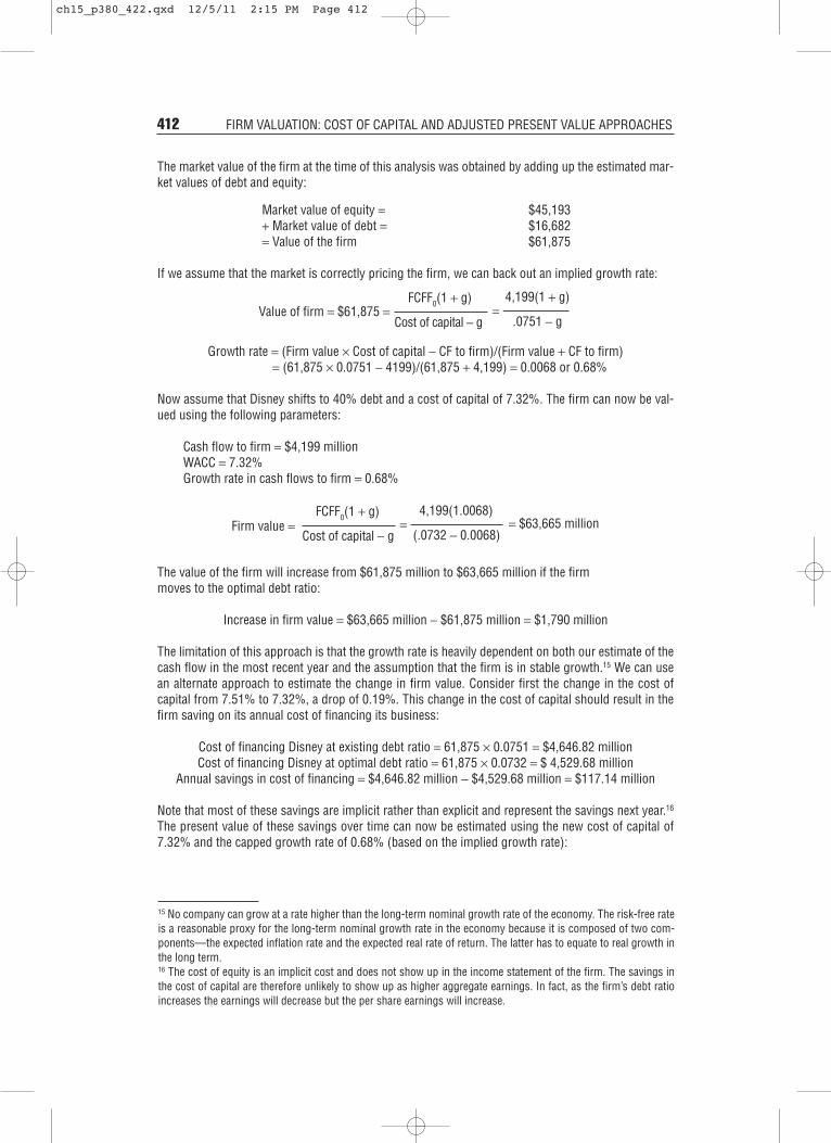
The market value of the firm at the time of this analysis was obtained by adding up the estimated mar-ket values of debt and equity:

Market value of equity = $45,193+ Market value of debt = $16,682= Value of the firm $61,875

If we assume that the market is correctly pricing the firm, we can back out an implied growth rate:

Growth rate = (Firm value × Cost of capital − CF to firm)/(Firm value + CF to firm)= (61,875 × 0.0751 − 4199)/(61,875 + 4,199) = 0.0068 or 0.68%

Now assume that Disney shifts to 40% debt and a cost of capital of 7.32%. The firm can now be val-ued using the following parameters:

Cash flow to firm = $4,199 millionWACC = 7.32%Growth rate in cash flows to firm = 0.68%

The value of the firm will increase from $61,875 million to $63,665 million if the firmmoves to the optimal debt ratio:

Increase in firm value = $63,665 million − $61,875 million = $1,790 million

The limitation of this approach is that the growth rate is heavily dependent on both our estimate of thecash flow in the most recent year and the assumption that the firm is in stable growth.15 We can usean alternate approach to estimate the change in firm value. Consider first the change in the cost ofcapital from 7.51% to 7.32%, a drop of 0.19%. This change in the cost of capital should result in thefirm saving on its annual cost of financing its business:

Cost of financing Disney at existing debt ratio = 61,875 × 0.0751 = $4,646.82 millionCost of financing Disney at optimal debt ratio = 61,875 × 0.0732 = $ 4,529.68 million

Annual savings in cost of financing = $4,646.82 million − $4,529.68 million = $117.14 million

Note that most of these savings are implicit rather than explicit and represent the savings next year.16

The present value of these savings over time can now be estimated using the new cost of capital of7.32% and the capped growth rate of 0.68% (based on the implied growth rate):

Firm value =FCFF0(1 + g)

Cost of capital − g

4,199(1.0068)

(.0732 − 0.0068)= = $63,665 million

Value of firm = $61,875 =FCFF0(1 + g)

Cost of capital − g

4,199(1 + g)

.0751 − g=

412 FIRM VALUATION: COST OF CAPITAL AND ADJUSTED PRESENT VALUE APPROACHES

15 No company can grow at a rate higher than the long-term nominal growth rate of the economy. The risk-free rateis a reasonable proxy for the long-term nominal growth rate in the economy because it is composed of two com-ponents—the expected inflation rate and the expected real rate of return. The latter has to equate to real growth inthe long term.16 The cost of equity is an implicit cost and does not show up in the income statement of the firm. The savings inthe cost of capital are therefore unlikely to show up as higher aggregate earnings. In fact, as the firm’s debt ratioincreases the earnings will decrease but the per share earnings will increase.

ch15_p380_422.qxd 12/5/11 2:15 PM Page 412

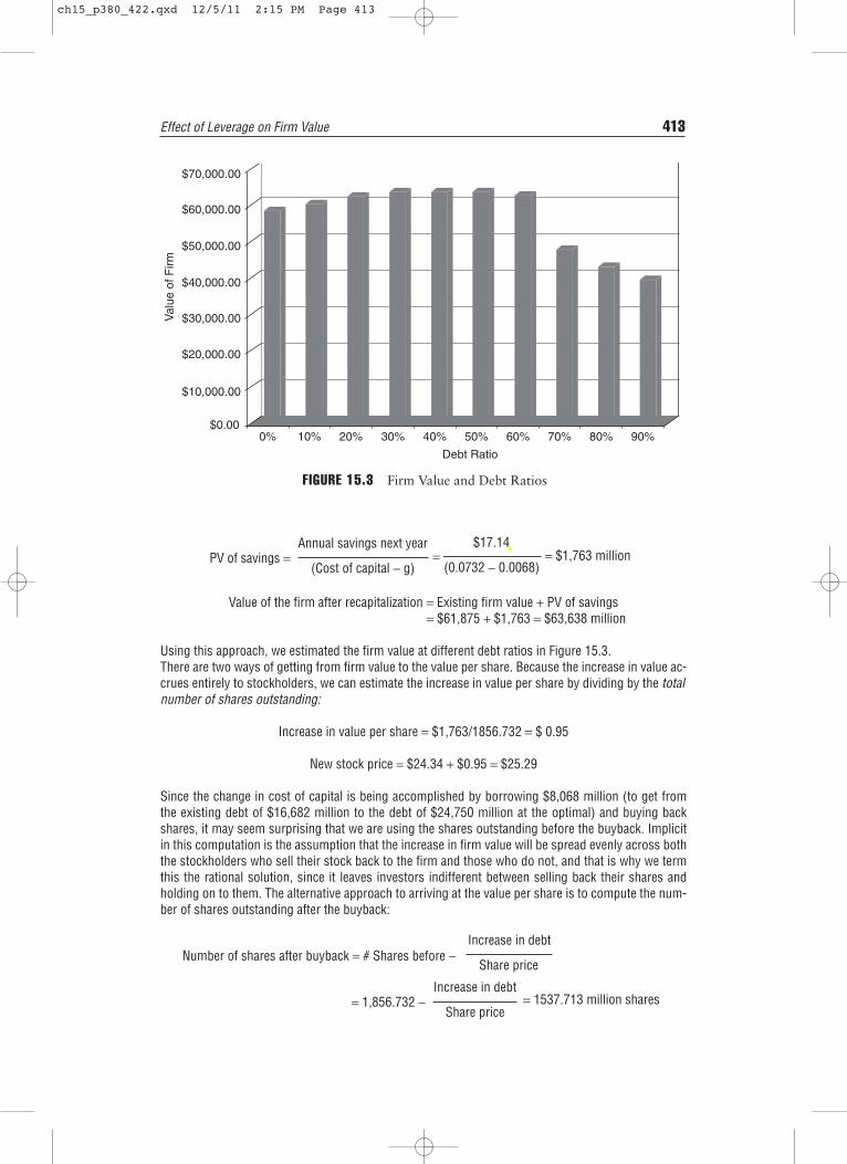
Value of the firm after recapitalization = Existing firm value + PV of savings = $61,875 + $1,763 = $63,638 million

Using this approach, we estimated the firm value at different debt ratios in Figure 15.3.There are two ways of getting from firm value to the value per share. Because the increase in value ac-crues entirely to stockholders, we can estimate the increase in value per share by dividing by the totalnumber of shares outstanding:

Increase in value per share = $1,763/1856.732 = $ 0.95

New stock price = $24.34 + $0.95 = $25.29

Since the change in cost of capital is being accomplished by borrowing $8,068 million (to get fromthe existing debt of $16,682 million to the debt of $24,750 million at the optimal) and buying backshares, it may seem surprising that we are using the shares outstanding before the buyback. Implicitin this computation is the assumption that the increase in firm value will be spread evenly across boththe stockholders who sell their stock back to the firm and those who do not, and that is why we termthis the rational solution, since it leaves investors indifferent between selling back their shares andholding on to them. The alternative approach to arriving at the value per share is to compute the num-ber of shares outstanding after the buyback:

= 1,856.732 −Increase in debt

Share price= 1537.713 million shares

Number of shares after buyback = # Shares before −Increase in debt

Share price

PV of savings =Annual savings next year

(Cost of capital − g)

$17.14

(0.0732 − 0.0068)= = $1,763 million

Effect of Leverage on Firm Value 413

FIGURE 15.3 Firm Value and Debt Ratios

0% 10% 20% 30% 40%

Debt Ratio

Val

ue o

f Firm

50% 60% 70% 80% 90%$0.00

$10,000.00

$20,000.00

$30,000.00

$40,000.00

$50,000.00

$60,000.00

$70,000.00

ch15_p380_422.qxd 12/5/11 2:15 PM Page 413

Value of firm after recapitalization = $63,638 millionDebt outstanding after recapitalization = $24,750 millionValue of equity after recapitalization = $38,888 million

To the extent that stock can be bought back at the current price of $24.34 or some value lower than$25.29, the remaining stockholders will get a bigger share of the increase in value. For instance, ifDisney could have bought stock back at the existing price of $24.34, the increase in value per sharewould be $1.16.17 If the stock buyback occurs at a price higher than $25.29, investors who sell theirstock back will gain at the expense of those who remain stockholder in the firm.

Value of equity per share after recapitalization =38,888

1537.713= $25.29

414 FIRM VALUATION: COST OF CAPITAL AND ADJUSTED PRESENT VALUE APPROACHES

captstr.xls: This spreadsheet allows you to compute the optimal debt ratio firmvalue for any firm, using the same information used for Boeing. It has updatedinterest coverage ratios and default spreads built in.

17To compute this change in value per share, we first compute how many shares we would buy back with the addi-tional debt taken on of $ 8,068 million (debt at 40% optimal of $24,750 million – Current debt of $16,682 million)and the stock price of $24.34. We then divide the increase in firm value of $1,763 million by the remaining sharesoutstanding:

Change in stock price = $1,763 million/(− [8068/24.34]) = $1.16 per share

Disney: Cost of Capital Worksheet

D/(D+E) 0.00% 10.00% 20.00% 30.00% 40.00% 50.00% 60.00% 70.00% 80.00% 90.00%

D/E 0.00% 11.11% 25.00% 42.86% 66.67% 100.00% 150.00% 233.33% 400.00% 900.00%

$ Debt $0 $6,188 $12,375 $18,563 $24,750 $30,938 $37,125 $43,313 $49,500 $55,688

Beta 0.73 0.78 0.85 0.93 1.04 1.19 1.42 1.79 2.55 5.05

Cost of Equity 7.90% 8.20% 8.58% 9.07% 9.72% 10.63% 11.99% 14.26% 18.81% 33.83%

EBITDA $8,422 $8,422 $8,422 $8,422 $8,422 $8,422 $8,422 $8,422 $8,422 $8,422

Depreciation $1,593 $1,593 $1,593 $1,593 $1,593 $1,593 $1,593 $1,593 $1,593 $1,593

EBIT $6,829 $6,829 $6,829 $6,829 $6,829 $6,829 $6,829 $6,829 $6,829 $6,829

Interest $0 $294 $588 $975 $1,485 $2,011 $2,599 $5,198 $6,683 $7,518

Interest ∞ 23.24 11.62 7.01 4.60 3.40 2.63 1.31 1.02 0.91coverage ratio

Likely Rating AAA AAA AAA AA A A- BBB B- CCC CCC

Pre-tax cost 4.75% 4.75% 4.75% 5.25% 6.00% 6.50% 7.00% 12.00% 13.50% 13.50%of debt

Effective 38.00% 38.00% 38.00% 38.00% 38.00% 38.00% 38.00% 38.00% 38.00% 34.52%tax rate

Cost of Capital Calculations

D/(D+E) 0.00% 10.00% 20.00% 30.00% 40.00% 50.00% 60.00% 70.00% 80.00% 90.00%

D/E 0.00% 11.11% 25.00% 42.86% 66.67% 100.00% 150.00% 233.33% 400.00% 900.00%

$ Debt $0 $6,188 $12,375 $18,563 $24,750 $30,938 $37,125 $43,313 $49,500 $55,688

Cost of equity 7.90% 8.20% 8.58% 9.07% 9.72% 10.63% 11.99% 14.26% 18.81% 33.83%

Cost of debt 2.95% 2.95% 2.95% 3.26% 3.72% 4.03% 4.34% 7.44% 8.37% 8.84%

Cost of capital 7.90% 7.68% 7.45% 7.32% 7.32% 7.33% 7.40% 9.49% 10.46% 11.34%

ch15_p380_422.qxd 12/5/11 2:15 PM Page 414

ADJUSTED PRESENT VALUE AND FINANCIAL LEVERAGE

In the adjusted present value (APV) approach, we begin with the value of the firmwithout debt. As we add debt to the firm, we consider the net effect on value byconsidering both the benefits and the costs of borrowing. The value of the leveredfirm can then be estimated at different levels of the debt, and the debt level thatmaximizes firm value is the optimal debt ratio.

Steps in the Adjusted Present Value Approach

The unlevered firm value is not a function of expected leverage and can be esti-mated as described in the earlier section—by discounting the free cash flows to thefirm at the unlevered cost of equity. In fact, if you do not want to estimate thisvalue and take the market value of the firm as correct, you could back out the un-levered firm value by subtracting out the tax benefits and adding back the expectedbankruptcy cost from the existing debt.

Current firm value = Value of unlevered firm + Present value of tax benefits − Expected bankruptcy cost

Value of unlevered firm = Current firm value − Present value of tax benefits + Expected bankruptcy cost

Adjusted Present Value and Financial Leverage 415

DEFAULT RISK, OPERATING INCOME, AND OPTIMAL LEVERAGE

The Boeing analysis just completed assumed that operating income would re-main constant while the debt ratios changed. While this assumption simplifiesthe analysis substantially, it is not realistic. The operating income, for manyfirms, will drop as the default risk increases; this, in fact, is the cost we label asan indirect bankruptcy cost. The drop is likely to become more pronounced asthe default risk falls below an acceptable level; for instance, a bond rating be-low investment grade may trigger significant losses in revenues and increasesin expenses.

A general model for optimal capital structure would allow both operatingincome and cost of capital to change as the debt ratio changes. We have al-ready described how we can estimate cost of capital at different debt ratios,but we could also attempt to do the same with operating income. For in-stance, we could estimate how the operating income for the Boeing wouldchange as debt ratios and default risk changes by looking at the effects of rat-ing downgrades on the operating income of other retailers.

If both operating income and cost of capital change, the optimal debt ra-tio may no longer be the point at which the cost of capital is minimized. In-stead, the optimal has to be defined as that debt ratio at which the value of thefirm is maximized.

ch15_p380_422.qxd 12/5/11 2:15 PM Page 415

The only components that change as a firm changes its leverage are the ex-pected tax benefits and the expected bankruptcy costs. To obtain these values asyou change leverage, you would go through the following five steps:

1. Estimate the dollar debt outstanding at each debt ratio. This process mirrorswhat was done in the cost of capital approach. Keeping firm value fixed, con-sider how much debt the firm will have at 20 percent debt, 30 percent debt,and so on.

2. Estimate the tax benefits of debt by multiplying the dollar debt by the tax rate.This essentially assumes that the debt is permanent and that the tax benefitswill continue in perpetuity.

3. Estimate the rating, interest rate, and interest expense at each debt ratio. Thisprocess again replicates what was done in the cost of capital approach.

4. Use the rating to estimate a probability of default. Note that Table 15.2 pro-vides these probabilities for each rating.

5. Estimate the expected bankruptcy cost by multiplying the probability ofbankruptcy by the bankruptcy cost, stated as a percent of unlevered firmvalue.

We compute the value of the levered firm at different levels of debt. The debt levelthat maximizes the value of the levered firm is the optimal debt ratio.

ILLUSTRATION 15.8: APV Approach to Optimal Capital Structure: Disney in March 2009

The APV approach can be applied to estimating the optimal capital structure for Disney. The firststep is to estimate the value of the unlevered firm. To do so, we start with the firm value of Disneyin 2009 and net out the effect of the tax savings and bankruptcy costs arising from the existingdebt.

Current market value of Disney = Value of equity + Value of debt = $45,193 + $16,682 = $61,875 million

We first compute the present value of the tax savings from the existing debt, assuming that the inter-est payment on the debt constitutes a perpetuity, using a marginal tax rate for Disney of 38%.

PV of tax savings from existing debt = Existing debt × Tax rate = $16,682 × 0.38 = $6,339 million

Based on Disney’s current rating of A, we estimate a probability of bankruptcy of 0.66% from Table8.19. The bankruptcy cost is assumed to be 25% of the firm value, prior to the tax savings. Allow-ing for a range of 10–40% for bankruptcy costs, we have put Disney’s exposure to expected bank-ruptcy costs in the middle of the range. There are some businesses that Disney is in where theperception of distress can be damaging—theme parks, for instance—but the movie and broadcast-ing businesses are less likely to be affected because projects tend be shorter-term and on a smallerscale.

PV of expected bankruptcy cost = Probability of default × Bankruptcy cost= 0.66% × (0.25 × 61,875) = $ 102 million

416 FIRM VALUATION: COST OF CAPITAL AND ADJUSTED PRESENT VALUE APPROACHES

ch15_p380_422.qxd 12/5/11 2:15 PM Page 416

We then compute the value of Disney as an unlevered firm.

Value of Disney as an unlevered firm = Current market value − PV of tax savings + Expected bankruptcy costs = $61,875 − $6,339 + $102= $55,638 million

The next step in the process is to estimate the tax savings in the following table at different levelsof debt. Although we use the standard approach of assuming that the present value is calculated as aperpetuity, we reduce the tax rate used in the calculation, if interest expenses exceed the EBIT. The ad-justment to the tax rate was described earlier in the cost of capital approach.

Tax Savings from Debt (tcD): Disney

Debt Ratio $ Debt Tax Rate Tax Benefits0% $ 0 38.00% $ 0

10% $ 6,188 38.00% $ 2,35120% $12,375 38.00% $ 4,70330% $18,563 38.00% $ 7,05440% $24,750 38.00% $ 9,40550% $30,938 38.00% $11,75660% $37,125 38.00% $14,10870% $43,313 38.00% $16,45980% $49,500 38.00% $18,81090% $55,688 34.52% $19,223

The final step in the process is to estimate the expected bankruptcy cost, based on the bond ratings,the probabilities of default, and the assumption that the bankruptcy cost is 25% of firm value. Thefollowing table summarizes these probabilities and the expected bankruptcy cost, computed based onthe levered firm value:

Expected Bankruptcy Cost, Disney

Debt Ratio Bond Rating Probability of Default Expected Bankruptcy Cost0% AAA 0.07% $ 10

10% AAA 0.07% $ 1020% AAA 0.07% $ 1130% A+ 0.60% $ 9440% A 0.66% $ 10750% A– 2.50% $ 42160% B 36.80% $ 6,41770% CCC 59.01% $10,63680% CCC 59.01% $10,98390% CCC 59.01% $11,044

The expected bankruptcy cost at a 40% debt ratio is computed thus:

Expected bankruptcy cost = (Unlevered firm value + Tax savings)(.25)(.0066)= (55,638 + $9,405)(.25)(0.0066) = $ 107 million

The value of the levered firm is estimated in the following table by aggregating the effects of the taxsavings and the expected bankruptcy costs.

Adjusted Present Value and Financial Leverage 417

ch15_p380_422.qxd 12/5/11 2:15 PM Page 417

Value of Disney with Leverage

Debt Tax Unlevered Tax Expected Value ofRatio $ Debt Rate Firm Value Benefits Bankruptcy Cost Levered Firm0% $ 0 38.00% $55,638 $ 0 $ 10 $55,629

10% $ 6,188 38.00% $55,638 $ 2,351 $ 10 $57,97920% $12,375 38.00% $55,638 $ 4,703 $ 11 $60,33030% $18,563 38.00% $55,638 $ 7,054 $ 94 $62,59840% $24,750 38.00% $55,638 $ 9,405 $ 107 $64,93650% $30,938 38.00% $55,638 $11,756 $ 421 $66,97360% $37,125 38.00% $55,638 $14,108 $ 6,417 $63,32970% $43,313 38.00% $55,638 $16,459 $10,636 $61,46180% $49,500 38.00% $55,638 $18,810 $10,983 $63,46690% $55,688 34.52% $55,638 $19,223 $11,044 $63,817

The firm value is maximized at about 50% debt, slightly higher than the optimal computed using thecost of capital approach. These results are, however, very sensitive to both the estimate of bankruptcycost as a percent of firm value and the probabilities of default.

418 FIRM VALUATION: COST OF CAPITAL AND ADJUSTED PRESENT VALUE APPROACHES

apv.xls: This spreadsheet allows you to compute the value of a firm, with leverage,using the adjusted present value approach.

VALUING THE PIECES RATHER THAN THE WHOLE

The adjusted present value model values debt separately from the operatingassets, and firm value is the sum of the two components. In fact, one of thebiggest benefits of discounted cash flow valuation is that breaking up cashflows into individual components and valuing them separately should notchange the value. Thus, you could value a firm like General Electric (GE) byvaluing each of its divisions separately and adding them up, or Coca-Cola byvaluing its operations in each country separately and summing those up.

The advantage of piecewise valuation is that you can estimate cash flowsand discount rates separately for each piece and thus get more precise esti-mates of value. For example, you would use very different assumptions aboutoperating margins, reinvestment needs, and costs of capital when valuing theappliance and aircraft engine divisions of GE. Similarly, you could apply dif-ferent country risk premiums for each country that Coca-Cola operates in tovalue the firm. Since this is always the case, you might ask why we do not dothis for all firms. The problem is with the information. Many firms do notbreak down their earnings and cash flows in sufficient detail to allow forpiecewise valuation. Even firms that do, like GE, often have large centralizedexpenses that get allocated, often arbitrarily, to individual divisions.

The benefits of breaking a firm down into pieces clearly increase as a firmbecomes more diverse in its operations. These benefits have to be weighedagainst the costs associated with more imprecise information and greater esti-mation problems.

ch15_p380_422.qxd 12/5/11 2:15 PM Page 418

Benefits and Limitations of the Adjusted Present Value Approach

The advantage of the APV approach is that it separates the effects of debt into dif-ferent components and allows the analyst to use different discount rates for eachcomponent. In addition, we do not assume that the debt ratio stays unchanged forever, which is an implicit assumption in the cost of capital approach. Instead, wehave the flexibility to keep the dollar value of debt fixed and to calculate the bene-fits and costs of the fixed dollar debt.

These advantages have to be weighed against the difficulty of estimating proba-bilities of default and the cost of bankruptcy. In fact, many analyses that use the ad-justed present value approach ignore the expected bankruptcy costs, leading them tothe conclusion that firm value increases as firms borrow money. Not surprisingly, thiswill yield the conclusion that the optimal debt ratio for a firm is 100 percent debt.

In general, with the same assumptions, the APV and the cost of capital conclu-sions give identical answers. However, the APV approach is more practical whenfirms are evaluating a dollar amount of debt, while the cost of capital approach iseasier when firms are analyzing debt proportions.18

CONCLUSION

This chapter develops an alternative approach to discounted cash flow valua-tion. The cash flows to the firm are discounted at the weighted average cost ofcapital to obtain the value of the firm, which when reduced by the market valueof outstanding debt yields the value of equity. Since the cash flow to the firm is a cash flow prior to debt payments, this approach is more straightforward to use when there is significant leverage or when leverage changes over time,though the weighted average cost of capital, used to discount free cash flows tothe firm, has to be adjusted for changes in leverage. Finally, the costs of capitalcan be estimated at different debt ratios and used to estimate the optimal debtratio for a firm.

The alternative approach to firm valuation is the APV approach, where the ef-fect on value of debt (tax benefits minus bankruptcy costs) is added to the unlev-ered firm value. This approach can also be used to estimate the optimal debt ratiofor the firm.

QUESTIONS AND SHORT PROBLEMS

In the problems following, use an equity risk premium of 5.5 percent if none isspecified. 1. Respond true or false to the following statements about the free cash flow to the

firm:a. The free cash flow to the firm is always higher than the free cash flow to equity.

True ____ False ____

Questions and Short Problems 419

18See Inselbag and Kaufold (1997).

ch15_p380_422.qxd 12/5/11 2:15 PM Page 419

b. The free cash flow to the firm is the cumulated cash flow to all investors inthe firm, though the form of their claims may be different.True ____ False ____

c. The free cash flow to the firm is a predebt, pretax cash flow.True ____ False ____

d. The free cash flow to the firm is an after-debt, after-tax cash flow.True ____ False ____

e. The free cash flow to the firm cannot be estimated for a firm with debt with-out knowing interest and principal payments.True ____ False ____

2. Union Pacific Railroad reported net income of $770 million in 1993 after inter-est expenses of $320 million. (The corporate tax rate was 36%.) It reported de-preciation of $960 million in that year, and capital spending was $1.2 billion.The firm also had $4 billion in debt outstanding on the books, rated AA (carry-ing a yield to maturity of 8%) and trading at par (up from $3.8 billion at theend of 1992). The beta of the stock was 1.05, and there were 200 million sharesoutstanding (trading at $60 per share), with a book value of $5 billion. UnionPacific’s working capital requirements were negligible. (The Treasury bond ratewas 7%, and the risk premium was 5.5%.)a. Estimate the free cash flow to the firm in 1993.b. Estimate the value of the firm at the end of 1993.c. Estimate the value of equity at the end of 1993, and the value per share, using

the FCFF approach.3. Lockheed Corporation, one of the largest defense contractors in the United

States, reported EBITDA of $1,290 million in 1993, prior to interest expenses of$215 million and depreciation charges of $400 million. Capital expenditures in1993 amounted to $450 million, and working capital was 7% of revenues(which were $13,500 million). The firm had debt outstanding of $3.068 billion(in book value terms), trading at a market value of $3.2 billion and yielding apretax interest rate of 8%. There were 62 million shares outstanding, trading at$64 per share, and the most recent beta was 1.10. The tax rate for the firm was40%. (The Treasury bond rate was 7%, and the risk premium was 5.5%.)

The firm expected revenues, earnings, capital expenditures and deprecia-tion to grow at 9.5% a year from 1994 to 1998, after which the growth ratewas expected to drop to 4%. (Capital spending will be 120% of depreciationin the steady state period.) The company also planned to lower its debt/equityratio to 50% for the steady state (which will result in the pretax interest ratedropping to 7.5%).a. Estimate the value of the firm.b. Estimate the value of the equity in the firm, and the value per share.

4. In the face of disappointing earnings results and increasingly assertive institu-tional stockholders, Eastman Kodak was considering a major restructuring in1993. As part of this restructuring, it was considering the sale of its health divi-sion, which earned $560 million in earnings before interest and taxes in 1993,on revenues of $5.285 billion. The expected growth in earnings was expected tomoderate to 6% between 1994 and 1998, and to 4% after that. Capital expen-ditures in the health division amounted to $420 million in 1993, while deprecia-tion was $350 million. Both were expected to grow 4% a year in the long term.Working capital requirements were negligible.

420 FIRM VALUATION: COST OF CAPITAL AND ADJUSTED PRESENT VALUE APPROACHES

ch15_p380_422.qxd 12/5/11 2:15 PM Page 420

The average beta of firms competing with Eastman Kodak’s health divisionwas 1.15. While Eastman Kodak had a debt ratio [D/(D + E)] of 50%, the healthdivision could sustain a debt ratio [D/(D + E)] of only 20%, which was similar tothe average debt ratio of firms competing in the health sector. At this level ofdebt, the health division could expect to pay 7.5% on its debt, before taxes. (Thetax rate is 40%, the Treasury bond rate is 7%, and the risk premium is 5.5%.)a. Estimate the cost of capital for the division.b. Estimate the value of the division.c. Why might an acquirer pay more than this estimated value for the division?

5. You are analyzing a valuation done on a stable firm by a well-known analyst.Based on the expected free cash flow to firm next year of $30 million and an ex-pected growth rate of 5%, the analyst has estimated a value of $750 million.However, he has made the mistake of using the book values of debt and equityin his calculation. While you do not know the book value weights he used, youknow that the firm has a cost of equity of 12% and an after-tax cost of debt of6%. You also know that the market value of equity is three times the book valueof equity, while the market value of debt is equal to the book value of debt. Esti-mate the correct value for the firm.

6. Santa Fe Pacific, a major rail operator with diversified operations, had earn-ings before interest, taxes, and depreciation of $637 million in 1993, with de-preciation amounting to $235 million (offset by capital expenditure of anequivalent amount). The firm was in steady state and expected to grow 6% ayear in perpetuity. Santa Fe Pacific had a beta of 1.25 in 1993, and debt out-standing of $1.34 billion. The stock price was $18.25 at the end of 1993, andthere were 183.1 million shares outstanding. The expected ratings and thecosts of debt at different levels of debt for Santa Fe are shown in the follow-ing table:

D/(D + E) Rating Cost of Debt (Pretax)

0% AAA 6.23%10% AAA 6.23%20% A+ 6.93%30% A– 7.43%40% BB 8.43%50% B+ 8.93%60% B– 10.93%70% CCC 11.93%80% CCC 11.93%90% CC 13.43%

The earnings before interest and taxes were expected to grow 3% a year in per-petuity, with capital expenditures offset by depreciation. (The tax rate is 40%,and the Treasury bond rate is 7% and the market risk premium is 5.5%.)a. Estimate the cost of capital at the current debt ratio.b. Estimate the costs of capital at debt ratios ranging from 0% to 90%.c. Estimate the value of the firm at debt ratios ranging from 0% to 90%.

7. You have been asked to estimate the value of Cavanaugh Motels, a motel chain.The firm reported earnings of $200 million before interest and taxes in the mostrecent year and paid 40% of its taxable income in taxes. The book value of

Questions and Short Problems 421

ch15_p380_422.qxd 12/5/11 2:15 PM Page 421

capital at the firm is $1.2 billion, and the firm expects to grow 4% a year in per-petuity. The firm has a beta of 1.2, a pretax cost of debt of 6%, equity with amarket value of $1 billion, and debt with a market value of $500 million. (Therisk-free rate is 5%, and the market risk premium is 5.5%.)a. Estimate the value of the firm, using the cost of capital approach.b. If you were told the probability of default at this firm at its current debt level

is 10% and that the cost of bankruptcy is 25% of unlevered firm value, esti-mate the value of the firm using the adjusted present value approach.

c. How would you reconcile the two estimates of value?8. Bethlehem Steel, one of the oldest and largest steel companies in the United

States, is considering the question of whether it has any excess debt capacity. Thefirm has $527 million in market value of debt outstanding and $1.76 billion inmarket value of equity. The firm has earnings before interest and taxes of $131million, and faces a corporate tax rate of 36%. The company’s bonds are ratedBBB, and the cost of debt is 8%. At this rating, the firm has a probability of de-fault of 2.3%, and the cost of bankruptcy is expected to be 30% of firm value.a. Estimate the unlevered value of the firm from the current market value of the

firm.b. Estimate the levered value of the firm, using the adjusted present value ap-

proach, at a debt ratio of 50%. At that debt ratio, the firm’s bond rating willbe CCC, and the probability of default will increase to 46.61% of unleveredfirm value.

422 FIRM VALUATION: COST OF CAPITAL AND ADJUSTED PRESENT VALUE APPROACHES

ch15_p380_422.qxd 12/5/11 2:15 PM Page 422