adjustment costs, firm responses, and micro vs. macro labor
TRANSCRIPT

Adjustment Costs, Firm Responses, andMicro vs. Macro Labor Supply Elasticities:
Evidence from Danish Tax RecordsThe Harvard community has made this
article openly available. Please share howthis access benefits you. Your story matters
Citation Chetty, Raj, John N. Friedman, Tore Olsen, and Luigi Pistaferri. 2011.Adjustment Costs, Firm Responses, and Micro vs. Macro LaborSupply Elasticities: Evidence from Danish Tax Records. QuarterlyJournal of Economics 126(2): 749-804.
Published Version http://dx.doi.org/10.1093/qje/qjr013
Citable link http://nrs.harvard.edu/urn-3:HUL.InstRepos:9639984
Terms of Use This article was downloaded from Harvard University’s DASHrepository, and is made available under the terms and conditionsapplicable to Other Posted Material, as set forth at http://nrs.harvard.edu/urn-3:HUL.InstRepos:dash.current.terms-of-use#LAA

ADJUSTMENT COSTS, FIRM RESPONSES, ANDMICRO VS. MACRO LABOR SUPPLY ELASTICITIES:
EVIDENCE FROM DANISH TAX RECORDS∗
RAJ CHETTY
JOHN N. FRIEDMAN
TORE OLSEN
LUIGI PISTAFERRI
We show that the effects of taxes on labor supply are shaped by interactionsbetween adjustment costs for workers and hours constraints set by firms. We de-velopa model in which firms post joboffers characterizedby an hours requirementand workers pay search costs to find jobs. We present evidence supporting threepredictions of this model byanalyzingbunchingat kinks usingDanishtaxrecords.First, larger kinks generate larger taxable income elasticities. Second, kinks thatapply toa larger group of workers generate larger elasticities. Third, the distribu-tion of job offers is tailoredtomatch workers’ aggregate tax preferences in equilib-rium. Our results suggest that macroelasticities may be substantially larger thanthe estimates obtained using standard microeconometric methods. JEL Codes:H20, J20.
I. INTRODUCTION
The vast theoretical and empirical literature on taxation andlabor supply generally assumes that workers can freely choosejobs that suit their preferences. This paper shows that the effectof taxes on labor supply is shaped by two factors that limit work-ers’ ability to make optimal choices: adjustment costs and hoursconstraints determined endogenously in equilibrium. We presentquasi-experimental evidence showing that these forces attenuatemicroeconometric estimates of labor supply elasticities.
To motivate our empirical analysis, we develop a stylizedlabor supply model with job search costs and endogenous hours
∗We would like to thank David Card, Stephen Coate, Edward Glaeser, JamesHines, Han Hong, Lawrence Katz, Henrik Kleven, Claus Kreiner, Patrick Kline,Erzo Luttmer, Robert Moffitt, John Pencavel, Emmanuel Saez, Laszlo Sandor,Esben Schultz, anonymous referees, and numerous seminar participants for help-ful suggestions and valuable discussion. We are extremely grateful to MetteEjrnæs and Bertel Schjerning at the Centre for Applied Microeconometrics at theUniversity of Copenhagen, Frederik Hansen at the Ministry of Finance, PeterElmer Lauritsen at Statistics Denmark, as well as Anders Frederiksen, PaulBingley, and Niels Chr. Westergard-Nielsen at Aarhus Business School for helpwith the data and institutional background. Gregory Bruich, Jane Choi, JessicaLaird, and Keli Liu provided outstanding research assistance. Support for thisresearch was provided by the Robert Wood Johnson Foundation and NSF GrantSES-0645396.
c© The Author(s) 2011. Published by Oxford University Press, on behalf of President andFellows of Harvard College. All rights reserved. For Permissions, please email: [email protected] Quarterly Journal of Economics (2011) 126, 749–804. doi:10.1093/qje/qjr013.
749
at Harvard U
niversity on September 26, 2012
http://qje.oxfordjournals.org/D
ownloaded from
750 QUARTERLY JOURNAL OF ECONOMICS
constraints. We model hours constraints by assuming that eachfirm requires its employees to work a fixed number of hours be-causeofanex-antecommitment toaproductiontechnology. Work-ers draw offers from the aggregate distribution of hours and cansearch for jobs that offer hours closer to their unconstrained opti-mumbypayingsearchcosts. Weconsidertwotypes of equilibriumin the labor market: competitive markets and collective bargain-ing. In the competitive case, both workers andfirms are price tak-ers. In the collective bargaining case – which is more relevant forour empirical application – unions bargain with firms over wagesand the aggregate hours distribution. Under both notions of equi-librium, the number of jobs posted by firms at each level of hoursmust equal thenumberofworkers whoselect thosehours afterthesearch process is complete. The aggregate distribution of workers’preferences therefore determines the hours constraints imposedby firms in equilibrium. However, most individuals do not worktheir unconstrained optimal number of hours because of searchcosts.
Ourmodel produces a divergencebetweenmacrolaborsupplyelasticities (definedas theeffect onaveragehours of workof varia-tion in taxes across economies) and microlabor supply elasticities(definedas the effect of tax changes or kinks in non-linear tax sys-tems that affect subgroups of workers). We show that the macroelasticity always equals the “structural” labor supply elasticityε, the parameter of individuals’ utility functions that determineselasticities absent frictions. In contrast, micro elasticities areattenuated relative to ε because of search costs and hoursconstraints.
The model generates three testable predictions about howsearch costs and hours constraints affect the labor supply (or tax-able income) elasticities observed in micro studies. All three pre-dictions holdirrespectiveof whetherthelabormarket equilibriumis determined by competition or collective bargaining. The firstprediction is that the observed elasticity increases with the sizeof the tax variation from which the estimate is identified. Intu-itively, large tax changes prompt more individuals to pay searchcosts and find a new job. Analogously, larger kinks induce moreindividuals topaysearchcosts tofinda jobthat places themat thekink. Second, theobservedelasticity increases withthenumberofworkers affectedby a tax change or kink. Changes in taxes inducechanges in labor supply not just by making individuals search fordifferent jobs, but also by changing the equilibrium distribution
at Harvard U
niversity on September 26, 2012
http://qje.oxfordjournals.org/D
ownloaded from
ADJUSTMENT COSTS AND LABOR SUPPLY ELASTICITIES 751
of hours. Because changes in taxes that affect a larger group ofindividuals induce larger changes in hours constraints – eitherthrough market forces or directly through unions – they gener-ate larger observed elasticities. Furthermore, tax changes mayaffect even the labor supply of workers whose personal tax in-centives are unchanged by distorting their coworkers’ incentivesand inducing changes in hours constraints. Finally, the modelpredicts a correlation between individual responses to tax andresponses to taxes induced by aggregation of workers’ tax prefer-ences through firms or unions. In particular, one should observelarger distortions in the equilibrium distribution of job offers insectors or occupations where workers themselves exhibit largertax elasticities.
We test these three predictions using a matched employer-employee panel of the population in Denmark between 1994 and2001. This dataset combines administrative records on earningsandtaxableincome, demographiccharacteristics, andemploymentcharacteristics such as occupation and tenure. There are twosources oftaxvariationinthedata: taxreforms across years, whichproducevariationinmarginal net-of-taxwagerates of 10% orless,and changes in tax rates across tax brackets within a year, whichgenerate variation in net-of-tax wages of up to 35%. We focus pri-marily on the cross-bracket variation in taxes rates because it islarger and applies to large subgroups of the population, permit-ting coordinated responses. In particular, we estimate taxable in-come elasticities by measuring the amount of bunching at kinkpoints, as in Saez (2010).1
Consistent with the first prediction, the elasticities impliedby the amount of bunching at large kinks are significantly largerthan those implied by the amount of bunching at smaller kinks.There is substantial, visually evident excess mass in the wageearnings distribution around the cutoff for the top income taxbracket in Denmark, at which the net-of-tax wage rate falls byapproximately 30%. There is little excess mass at kinks wherethe net-of-tax wage falls by 10%, andnoexcess mass at kinks thatgenerate variation in net-of-tax wages smaller than 10%.
1. Following the modern public finance literature reviewed in Saez, Slemrod,andGiertz (2009), weproxyfor“laborsupply”usingtaxableincome. Wediscuss theimplications of measuring taxable income elasticities instead of hours elasticitiesbelow.
at Harvard U
niversity on September 26, 2012
http://qje.oxfordjournals.org/D
ownloaded from

752 QUARTERLY JOURNAL OF ECONOMICS
Similarly, we find no changes in earnings around the small taxreforms that change net-of-tax wages by less than 10%. The ob-served elasticities at the largest kinks are several times largerthan those generated by smaller kinks and tax reforms across abroadrangeofdemographicgroups, occupations, andyears. Usingaseries ofauxiliarytests, weshowthat thedifferences inobservedelasticities are driven by differences in the size of the tax changesrather than heterogeneity in elasticities by income levels or taxrates.
To test the second prediction, we exploit heterogeneity in de-ductions across workers. In Denmark, 60% of wage earners havezero deductions. These workers reach the top tax bracket whentheir wage earnings exceeds the top tax cutoff for taxable income,which we term the “statutory” top tax cutoff. Workers with largedeductions or non-wage income, however, reach the top taxcutoffat different levels of wage earnings and thus have less com-mon tax incentives. We first demonstrate that firms and unionscater to the tax incentives of the most common workers. In par-ticular, the mode of occupation-level wage earnings distributionshas an excess propensity to be located near the statutory top taxcutoff.2 Importantly, the wage earnings distribution even forworkers whohave substantial deductions or non-wage income ex-hibits excess mass at the statutory top tax cutoff. Because theseworkers do not face any change in marginal tax rates at thestatutorycutoff, this findingconstitutes direct evidencethat wage-hours offers are tailored to the tax preferences of the majority ofworkers who have small deductions. We label this supply-side re-sponse to tax incentives induced by the aggregation of workers’tax preferences “aggregate bunching”.
Although aggregate bunching is an important source of be-havioral responses to the tax system, some of the bunching atkinks is driven by individual workers searching for jobs that placethem near the top tax kink. Toisolate and measure such “individ-ual bunching,” we exploit a cap on tax-deductible pension contri-butions, which is on average DKr 33,000 in the years we study.Approximately 3% of workers make pension contributions up tothis amount and therefore cross into the highest income tax
2. We focus on wage earnings distributions at the occupation level becausemost workers’ wages are set through collective bargains at the occupation level inDenmark.
at Harvard U
niversity on September 26, 2012
http://qje.oxfordjournals.org/D
ownloaded from

ADJUSTMENT COSTS AND LABOR SUPPLY ELASTICITIES 753
bracket when they earn DKr 33,000 more than the statutory toptax cutoff. We find that this pension-driven kink induces excessmass in the distribution of wage earnings at DKr 33,000 abovethe top tax cutoff. This excess mass appears tobe driven solely byindividual job search, as there is no excess mass at the pension-driven kink for workers with small deductions. Because of aggre-gate bunching, workers with common tax preferences (those withsmall deductions) havea higherpropensitytobunchat thetoptaxkink than those with uncommon tax preferences (those with largedeductions).
We test the third prediction by estimating the correlation be-tween individual and aggregate bunching across occupations. Wefind that there is more bunching at the statutory kink in occu-pations where workers exhibit more individual bunching in wageearnings at the pension-driven kink. Although this result cannotbe interpreted as a causal effect because the variation in indi-vidual bunching is not exogenous, it is consistent with the pre-diction that firms and unions cater to workers’ aggregate taxpreferences.
All of the results above are obtainedfor wage earners. We an-alyze self-employed individuals separately. As the self-employeddo not face significant adjustment costs or hours constraints, onewould expect that none of our three predictions should hold forthis subgroup. Indeed, wefindthat theself-employedexhibit sharpbunching at both small and large kinks, show no evidence of ag-gregate bunching at the statutory kink, and are equally likely tobunch irrespective of their deductions. These placebo tests sup-port our hypothesis that search costs and hours constraints arethe key factors that attenuate micro elasticity estimates for wageearners.
Although our findings show that adjustment costs and hoursconstraints are likely todampen observed elasticities, they donotidentify the underlying structural elasticity ε relevant for macrocomparisons. Identifying ε would require estimating a structuralmodel of labor supply with frictions and endogenous hours con-straints. Such an analysis is outside the scope of this paper, buttwo observations suggest that the structural elasticity ε is likelyto be an order of magnitude larger than the observed elastici-ties in our data, which are below 0.02. First, calibrations of ourstylized model consistently imply values of ε an order of magni-tude larger than the observed elasticities at the top kink (Chetty
at Harvard U
niversity on September 26, 2012
http://qje.oxfordjournals.org/D
ownloaded from

754 QUARTERLY JOURNAL OF ECONOMICS
et al. 2009). Second, theself employedexhibit muchlargertaxableincomeelasticities thanwageearners, suggestingthat individualsdo seek to optimize relative to taxes when they face fewerfrictions.3
Our results could help explain why macro studies find muchlarger elasticities than microeconometric studies (Blundell andMaCurdy 1999; Saez, Slemrod, and Giertz 2009; Chetty 2011).4
Microestimates areattenuatedbyfrictions becausetheyareiden-tified from individuals’ responses to changes in tax rates or kinksafter obtaining a job near their optimum. In contrast, macro vari-ation in tax rates across countries changes the jobs individualssearch for and the jobs offered by firms to begin with, produc-ing larger elasticities.5 Our explanation for the gap between mi-cro and macro elasticities complements recent work arguing thatmacroelasticities are larger because they incorporate both exten-siveandintensivemarginresponses (e.g. RogersonandWallenius2009). Much of the difference in labor supply across countrieswith different tax regimes is driven by hours worked conditionalon employment (Davis and Henrekson 2005; Chetty et al. 2011).That is, macroestimates of intensive margin elasticities are muchlargerthantheirmicroeconometriccounterparts. Ouranalysis ex-plains this divergence between intensive margin elasticities. Wecaution, however, that our findings do not provide justificationfor the very large elasticities (e.g. ε>1) used in some macromodels.
In addition to the literature on micro vs. macro elasticities,our study builds on and contributes to several other strands ofthe literature on labor supply. First, previous work has proposedthat adjustment costs and hours constraints affect labor supplydecisions (e.g. Cogan 1981; Ham 1982; Altonji and Paxson 1988;Dickens and Lundberg 1993; Rogerson 2005) and that long-run
3. This finding is consistent with a recent literature that documents largerelasticities for workers who can control their hours more easily, such as stadiumvendors (Oettinger1999), bikemessengers (FehrandGoette2007), andcabdrivers(Farber 2005).
4. A recent microeconometric study that uses the same Danish microdata aswe do here (Kleven and Schultz 2010) estimates an elasticity of zero by studyingtax reforms over a twenty year period.
5. Frictions could also explain why macro studies find large (Frisch) elastici-ties when analyzing fluctuations in labor supply over the business cycle. Intertem-poral wagefluctuations arelargeforcertainsubgroups andmuchof thefluctuationin hours at business cycle frequencies is on the extensive rather than intensivemargin (Chetty 2011).
at Harvard U
niversity on September 26, 2012
http://qje.oxfordjournals.org/D
ownloaded from

ADJUSTMENT COSTS AND LABOR SUPPLY ELASTICITIES 755
elasticities may differ from short-run elasticities (Holmlund andSoderstrom 2008).6 Our contribution is to show how these factorsaffect estimates of intensive-margin labor supply elasticities us-ing quasi-experimental methods. Our findings also support thehypothesis that the effects of government policies may operatethroughcoordinatedchanges insocial norms orinstitutions ratherthan individual behavior (e.g. Lindbeck 1995; Alesina, Glaeser,and Sacerdote 2005).
Second, our results contribute to the literature on non-linearbudget sets (e.g., Hausman 1981; Moffitt 1990; MaCurdy, Green,and Paarsch 1990), where the lack of bunching at kinks createsproblems in fitting models to the data. As noted by Blundell andMaCurdy (1999), “. . . for the vast majority of data sources cur-rently used in the literature, only a trivial number of individuals,if indeed any at all, report [earnings] at interior kink points.” Thekinks examined in previous studies are generally much smaller –both in the change in tax rates at the kink and the size of thegroup of individuals affected – than the largest kinks studiedhere.
Third, our analysis relates to recent work on taxable in-come as a measure of labor supply (Feldstein 1999; Slemrod andYitzhaki 2002; Chetty 2009). The bunching we observe is drivenby changes in wage earnings rather than tax avoidance via pen-sion contributions or evasion. However, because our dataset doesnot contain information on hours of work, we cannot rule out thepossibility that some of the responses we observe arise from in-come shifting. Importantly, distinguishing income shifting fromhours of work is not critical for the conclusions we draw here, asour three predictions also apply to an environment with adjust-ment costs and coordination constraints in income shifting.
The paper is organized as follows. In Section II, we set up themodel, define micro and macro elasticities formally, and derivethetestablepredictions. Section III describes theDanishdata andprovides institutional background. Section IV presents the empir-ical results. Section V concludes.
6. Our paper differs from the recent work of Chetty (2011) in two ways.First, while Chetty (2011) derives bounds on elasticities under the assumptionthat individuals face adjustment costs, we provide direct empirical evidence thatadjustment costs affect observed elasticities within a single economy. Second,Chetty (2011) focuses exclusively on worker behavior, while we model endogenoushours constraints and firm/union responses in equilibrium.
at Harvard U
niversity on September 26, 2012
http://qje.oxfordjournals.org/D
ownloaded from

756 QUARTERLY JOURNAL OF ECONOMICS
II. SEARCH COSTS AND HOURS CONSTRAINTS
IN A LABOR SUPPLY MODEL
This section develops a stylized model of labor supply on theintensive-margin whose purpose is to highlight the channelsthrough which frictions affect labor supply elasticities. We ana-lyze a static model because our empirical analysis focuses on howsearch costs and hours constraints interact in equilibrium ratherthan on the dynamics of adjustment in labor supply. We presentsomeresults onresponses totaxreforms ina two-periodextensionof this stylized model in Online Appendix A.7
II.A. Setup
Firms. Firms have one-factor linear production technologies.Each firm employs a single worker toproduce goods soldat a fixedprice p. Let w(h) denote the hourly wage rate paidtoworkers whowork h hours in equilibrium. Firm j posts a job that requires hj
hours of work at the wage rate w(hj). We model hours constraintsby assuming that a firm cannot change the hours it posts aftermatching with a worker.8 This assumption captures the intuitionthat firms sink capital in a technology that requires a certainamount of labor for production before hiring workers. Such con-straints may emerge from technological benefits of coordinatingwork schedules (as in an assembly line), the fixed costs of restruc-turing job and benefit packages, or regulations such as overtimepay requirements.9
A firm that posts a job with hj hours earns profit
πj = phj −w(hj)hj.
Let theaggregatedistributionof hours offeredbyfirms bedenotedby a cdf G (h). A key feature of our model is that the aggregate
7. All appendix material is available online at http://qje.oxfordjournals.org/.
8. This model is isomorphic to one in which a single firm offers heteroge-neous hours packages and workers face costs of switching jobs within the firm.This is because the boundary of a firm is indeterminate with constant returns toscale.
9. We focus on hours constraints in the model for simplicity, but they shouldbeinterpretedmorebroadlyas technological constraints onjobcharacteristics (e.g.training, effort, benefit packages).
at Harvard U
niversity on September 26, 2012
http://qje.oxfordjournals.org/D
ownloaded from

ADJUSTMENT COSTS AND LABOR SUPPLY ELASTICITIES 757
distributionof hours constraints G(h) is endogenously determinedin equilibrium, as we describe below.10
Workers. Workers, indexed by i, have quasi-linear utility
(1) ui (c, h) = c− α−1/εi
h1+1/ε
1 + 1/ε
over a numeraire consumption good c and hours of work h. Theheterogeneous taste parameter αi > 0, is distributed accordingto a smooth cdf F(αi) with full support on a closed interval. Thisutilityspecificationeliminates incomeeffects andgenerates a con-stant wage elasticity of labor supply ε in a frictionless model. Weabstract fromincomeeffects becausethevariationinmarginal taxrates at kinks that we exploit for identification has little effect onaveragetaxrates andthus generates negligibleincomeeffects. Weextendtheanalysis toutilityfunctions that generatenon-constantelasticities in Online Appendix A.
Tocharacterizetaxchanges that affect subgroups of thepopu-lation differently, assume that there are twotypes of tax systems,indexed by s ∈ {NL, L}.11 Individuals with si = NL face a two-bracket non-linear tax system with marginal tax rates of τ1 andτ2 > τ1. These workers begin topay the higher tax rate when theirincomes wihi exceed a threshold K. Individuals with si = L pay alinear tax rate of τ on all income. With this tax system, individuali has consumption
(2) ci(hi)=
(1− τ1)min (wihi, K)+(1− τ2)max (wihi − K, 0) if si = NL
(1− τ)wihi if si = L
A fraction ζ of workers face the non-linear tax system NL andthe remainder (1− ζ) face the linear tax system L. Let worker i’soptimal level of hours be denoted by h∗i = arg maxhi
ui (c (hi) , hi).The tax systems workers face are uncorrelated with their tastes:F(αi|si)= F(αi) .
10. This endogenous determination of wage-hours offers differentiates thismodel from the few existing models of hours constraints, in which firms’ technolo-gies exogenously determine the distribution of wage-hours packages (e.g. Rosen1976).
11. For example, tax systems often treat single and married individuals dif-ferently, in which case the two types in our model would be defined by maritalstatus.
at Harvard U
niversity on September 26, 2012
http://qje.oxfordjournals.org/D
ownloaded from

758 QUARTERLY JOURNAL OF ECONOMICS
Workers begin their search for a job by drawing an initialoffer h0
i from the aggregate offer distribution G(h). Each workercan either accept this offer or turn it down and search for anotherjob. We assume that workers who search locate their optimal jobh∗i , but must pay a utility cost of search φi. As a result, workerswill search for their optimal job if and only if the gains from theswitch are larger than φi. This job search process for workers canbe viewed as a functional F that maps an aggregate distributionof hours posted by firms G(h) and wage schedule w(h) to a newdistributionF(G(h) , w(h)).
II.B. Equilibrium
To demonstrate that our testable predictions apply to bothcompetitiveandunionizedlabormarkets suchas that ofDenmark,we analyze two different equilibrium concepts – one based oncollective bargaining and another based on market competition.
Model 1: Collective Bargaining. There is a single union thatrepresents all the workers in the economy. As in Earle and Pen-cavel (1990), we assume that the union bargains with firms overboth wages and hours, holding fixed the number of available jobs.Theunion’s objectiveis tomaximizeits members’ aggregateutilitysubject tothe constraint that all members must find jobs (full em-ployment). Since there are many firms and one union, the unionmakes a take-it-or-leave-it offertoall firms, whomayaccept orde-cline it individually. Theworkers thensearchfor jobs as describedabove. If there are more workers than firms at a given hours levelafter the search process, jobs are randomly rationed to workers,and hence some workers are unemployed.
In equilibrium, unions determine the wage and the distribu-tion of hours, subject to the constraints that firms must partici-pate in the labor market and all workers are employed. Becauselabor demand is infinitely elastic, firms will not accept w > p, andthe unions impose w = p. In order to satisfy the full employmentconstraint, the union must choose a distribution of jobs G (h) sat-isfying the fixed-point condition G∗ (h) =F (G∗(h) , p). This condi-tion ensures that the distribution of hours endogenously reflectstheaggregatedistributionof workerpreferences. If manyworkersprefer to work 40 hours per week, the union bargains to inducemany firms tooffer jobs that require 40 hours of labor per week inequilibrium.
at Harvard U
niversity on September 26, 2012
http://qje.oxfordjournals.org/D
ownloaded from
ADJUSTMENT COSTS AND LABOR SUPPLY ELASTICITIES 759
Model 2: Market Equilibrium. In a decentralized competitiveequilibrium, firms post anhours offerhj chosentomaximizeprofit:
(3) πj = phj −w(hj)hj.
Intuitively, firms seek to produce at an hours level where thesupply of labor exceeds demand, allowing them to earn profits bypaying a wage w(hj)< p. Because firms are free to enter the mar-ket at any level of hours hj, profits are bid to zero, implying thatw(hj) = w = p for all hj in equilibrium. Market clearing requiresthat thedistributionof jobs initiallypostedbyfirms coincides withthe jobs selected by workers at the wage rate w = p after the jobsearch process is complete, i.e. G∗(h)=F (G∗(h) , p).
Both the market equilibrium and collective bargaining mod-els generate a fixed wage w = p and a distribution of hours G∗(h)that endogenouslyreflects thepreferences ofworkers whileensur-ing full employment. The only difference between the two modelsis the mechanism through which worker preferences are aggre-gated to generate G(h): through firms in the market equilibriummodel and through unions in the collective bargaining model. Be-cause the twomodels generate the same equilibrium hours distri-bution, the predictions derived below apply to both institutionalstructures of the labor market. The two models of wage settingproduce the same equilibrium because our model assumes thatlabor demand is infinitely elastic. However, the key mechanismsthat drive our testable predictions would also operate in a morerealistic setting in which the labor demand elasticity is finite andunions extract rents. In particular, unions would continue to ag-gregate the tax preferences of the workers they represent, lead-ing to larger responses to tax changes that have large size andscope.
Our model should be viewed as representing the equilibriumin a given sector or occupation. It is straightforward to generateheterogeneous wage rates by introducing multiple sectors. Sup-pose there are Q different skill types of workers and Q types ofcorresponding output goods sold at prices p1, . . ., pQ. Workers oftype q can only work at firms that produce good q, so there isno interaction across the Q segments of the labor market. Withineach sector one union bargains with firms to set an equilibriumwage rate wq = pq and an equilibrium hours distributiondetermined by its workers’ preferences according to the modelabove.
at Harvard U
niversity on September 26, 2012
http://qje.oxfordjournals.org/D
ownloaded from

760 QUARTERLY JOURNAL OF ECONOMICS
The following sections characterize the properties of the equi-librium hours distribution G(h), focusing on the relationship be-tween tax rates and labor supply. For analytical convenience, wederive the key predictions in a series of special cases.
II.C. Special Case 1: Benchmark Frictionless Model
In the frictionless model (φi =0), the structural preference pa-rameter ε fully determines the effects of taxes on labor supply.This is because workers who face no search costs always choosetheir unconstrained optimal level of hours h∗i . For workers withsi = L, who face a linear tax τ , the optimal level of hours is h∗i =αi ((1− τ)w)
ε. The hours choices of workers who face the non-linear tax system are given by
(4) h∗i =
αi ((1− τ1)w)ε if αi < α
hK = Kw if αi ∈ [α,α]
αi ((1− τ2)w)ε if αi > α
whereα = hK/ ((1− τ1)w)ε andα = hK/ ((1− τ2)w)
ε. Workers withmoderate disutilities of labor supply αi ∈ [α,α] bunch at the kinkbecause the net-of-tax wage falls at hK .12
Now consider how variation in the linear tax rate τ affectslabor supply. When subject to a higher tax rate, workers of typesi = L optimally reduce their work hours by
(5) d logh = ε ∙ d log(1− τ) .
This equation shows that the elasticity of hours with respect tothe net-of-tax rate (1− τ) coincides with the structural parameterε in the frictionless model. We shall therefore refer to ε as the“structural” elasticity. Workers of type s = NL, whoare unaffectedby τ , do not change hours of work and can be used as a controlgroup in an empirical study.
In our one-dimensional labor supply model, the hours elas-ticity coincides with the elasticity of taxable wage income (wh)
12. The logic for why a mass of workers bunch at the kink is captured by thefollowingquotefroma Danishconstructionworkerinterviewedbya memberof theDanish Tax Reform Commission: “By the end of November, some of my colleaguesstop working. It does not pay anymore because they have reached the high taxbracket.”
at Harvard U
niversity on September 26, 2012
http://qje.oxfordjournals.org/D
ownloaded from
ADJUSTMENT COSTS AND LABOR SUPPLY ELASTICITIES 761
withrespect tothenet-of-tax-rate: ε= d logwhd log(1−τ). Inpractice, income
taxes may distort choices beyond hours of work, such as train-ing, effort, andfringe benefits. It is straightforwardtoincorporatesuchmargins intothemodel byassumingthat firms post joboffersthat specify H characteristics (or tasks),
−→h = (h1, . . ., hH), along
with wage rates −→w = (w1, . . ., wH) and workers have utility over-characteristics ψ(h1, . . ., hH). In such a model, the analysis that
follows applies to the taxable income elasticity ε= d log−→w ∙−→h
d log(1−τ) ratherthan the hours elasticity.
In the stylized models we consider here, the taxable incomeelasticityε is theparameterrelevant foranalyzingtaxpolicy(Feld-stein 1999). In a more general union bargaining model with a fi-nite labor demand elasticity, taxable income responses may bedriven partly by wage and employment changes. For example, inHansen’s (1999)model of taxationwithbargainingoverwages andworking hours, a higher marginal tax rate leads to lower wagerates, shorterworkinghours, andhigheremployment. Intuitively,when faced with an increase in tax rates, unions moderate theirwagedemands inexchangefora lowerunemployment level. Whilethe welfare implications of taxation would differ in such an envi-ronment, the three qualitative predictions derived below regard-ing the impact of frictions on observed responses to tax changeswould still apply.
The elasticity ε is most commonly estimated using variationin tax rates from tax reforms (Blundell and MaCurdy 1999; Saez,Slemrod, and Giertz 2009). However, ε can alsobe identified fromcross-sectional variation in tax rates using non-linear budget setmethods (e.g. Hausman 1981). In particular, the amount ofbunching observed at kinks identifies ε (Saez 2010). Let BNL =[F(α)−F(α) ] denote the fraction of type si = NL individuals whochoose hi = hK . Let gNL(hK) denote the counterfactual density ofhours in the absence of the tax change at the kink, which can bemeasured by the left limit of the density of the empirical hoursdistribution for type si = NL individuals in this simple model. Un-der the approximation that the hours distribution gNL is uniformaround the kink, Saez (2010) shows that
(6) ε 'BNL(τ1, τ2)/gNL(hK)
K ln(
1−τ11−τ2
) =bNL(τ1, τ2)
K ln(
1−τ11−τ2
) .
at Harvard U
niversity on September 26, 2012
http://qje.oxfordjournals.org/D
ownloaded from

762 QUARTERLY JOURNAL OF ECONOMICS
where bNL = BNL/gNL(hK) denotes the fraction of type si = NL in-dividuals whobunch at the kink normalizedby the counterfactualdensity. Intuitively, the fraction of individuals who stop workingat hi = hK hours because of the change in marginal tax rates isproportional to ε.
An important property of equations (5) and (6) is that the ob-served elasticity coincides with ε irrespective of the magnitude ofthe change in tax rates or the fraction of workers ζ affected bythe tax change.13 This result underlies microeconometric empir-ical studies of labor supply that use changes in taxes that affectsubgroups of the population to identify ε. We now show that withsearchcosts andhours constraints, observedelasticities varywiththe size and scope of tax changes and no longer coincide with ε.
II.D. Special Case 2: Search Costs and Worker Responses
In this subsection, we analyze the impact of search costs onbehavioral responses totaxation, abstracting from changes in thehours offered by firms. To isolate worker responses, we assumethat the set of workers affected by the tax change has measurezero. Whenanalyzingbunchingat kinks, weassumethat thefrac-tion of agents who face the non-linear tax system is ζ = 0; con-versely, when analyzing tax reforms, we assume ζ = 1. Under thisassumption, the tax change has no impact on the equilibrium of-fer distribution G(h) and only affects the treated workers’ hoursthrough changes in job search. To simplify notation, we assumethat all workers facethesamesearchcosts φi=φ; theresults belowdo not rely on this restriction.
Under these assumptions, a worker searches for a new job if
his initial offer h0i /∈
[hi, hi
], where the thresholds are defined by
the equations:
u (ci(h∗i ) , h∗i )− u (ci(hi) , hi) = φ with hi < h∗i(7)
u (ci(h∗i ) , h∗i )− u(
ci(hi) , hi
)= φ with hi > h∗i(8)
Workers whodrawhours that fall within the region[hi, hi
]retain
their initial offer because the utility gains from working h∗i hoursinstead of h0
i hours are less than the cost of search φ. After the
13. Weusetheterm“taxchange”toreferbothtochanges intaxrates overtimevia reforms and changes in marginal tax rates at kinks within a given period.
at Harvard U
niversity on September 26, 2012
http://qje.oxfordjournals.org/D
ownloaded from

ADJUSTMENT COSTS AND LABOR SUPPLY ELASTICITIES 763
search process is complete, there are twotypes of workers at eachfirm j: a point mass whose optimal labor supply h∗i = hj is exactlythat offeredbythefirmanda distributionof workers withoptimalhours near but not equal to hj.
Now consider how the mapping from the amount of bunch-ing at kinks to ε in (6) is affected by search costs. Let ε(τ1, τ2)=BNL(τ1,τ2)/gNL(hK )
K ln( 1−τ11−τ2 )
denote the elasticity obtainedby applying equation
(6). We shall refer to ε as the “observed” elasticity from bunchingat the kink. To understand the connection between ε and ε, firstrecall that in the frictionless model (where φ = 0), workers locateat the kink if αi ∈ [α,α]. When φ > 0, workers locate at the kink if
αi ∈ [α,α] and h0i /∈
[hi, hi
].14 As a result, the observed elasticity
ε is smaller than the structural elasticity ε. As the size of the taxchange at the kink increases (τ1 falls or τ2 rises), the set of work-ers withαi ∈ [α(τ1, τ2) ,α(τ1, τ2) ]whopay the search cost to locateat the kink expands:
(9)∂[hi − hi]
∂τ2< 0 and
∂[hi − hi]
∂τ1> 0.
Because the equilibrium hours distribution G(h) is not affectedby τ1 and τ2 when ζ = 0, it follows immediately that ε rises with
τ2 − τ1. As τ1 → −∞ and τ2 → ∞, the inaction region[hi, hi
]
collapses to hK for agents with αi ∈ [α,α] and ε→ ε. Larger kinksgenerate larger observed elasticities because the utility costs ofignoring a kink increase with its size. Figure I illustrates this in-tuition using indifference curves in consumption-labor space foran agent who would optimally set hours at hK . The thresholds[hi, hi
]are where the budget constraint crosses the indifference
curve that yields utility φ units less than the maximal utility U∗.Nowsuppose τ2 increases, movingtheupperbudget segment fromthe solid line to the dashed line. Then the upper bound hi de-creases, which in turn increases ε. This is because the utility lossfrom supplying hours above the kink rises with τ2, as one earns
14. Workers who draw h0i ∈
[hi, hi
]do not contribute to the point mass at the
kink because G(h) is smooth when ζ = 0. Therefore, among type si = NL workers,the set whodrawan initial hours offer h0
i = K/w has measure zero. G(h) is smoothin this case because the distribution of tastes F(α) is smooth and the set of agentswho face a smooth (linear) tax schedule has measure 1.
at Harvard U
niversity on September 26, 2012
http://qje.oxfordjournals.org/D
ownloaded from

764 QUARTERLY JOURNAL OF ECONOMICS
FIGURE IBunching at Kinks with Search Costs
This figure illustrates how search costs affect bunching at kinks. The two-bracket taxsystemcreates thekinkedbudget set shownindarkgray. Theworker’sindifference curves are shown by the light gray isoquants. This worker’s optimallabor supply is toset h∗=hK , placing him at the kink. The lower indifference curveshows the optimal utility minus the search cost φ. If the workers draws an initialhours offer between h and h , he will not pay φ torelocate tothe kink. As the taxchange at the bracket cutoff increases in magnitude (shown by the dashed line),the inaction region shrinks to ( h, h
′), leading to a larger observed elasticity from
bunching.
less for this extra effort. These results lead to our first testableprediction:
PREDICTION 1: Whenworkers facesearchcosts, theobservedelas-ticity from bunching rises with the size of the tax change andconverges to ε as the size of the tax change grows:
(10) ∂ε/∂τ2 > 0, ∂ε/∂τ1 < 0, and lim(τ2−τ1)→∞
ε = ε
at Harvard U
niversity on September 26, 2012
http://qje.oxfordjournals.org/D
ownloaded from

ADJUSTMENT COSTS AND LABOR SUPPLY ELASTICITIES 765
We derive an analogous prediction for observed elasticitiesfrom tax reforms in Online Appendix A. Tax reforms generate
observed elasticities ε = d log hd log(1−τ) that differ from ε; as the size of
the tax reform grows, ε → ε. The intuition for this result is verysimilartothat forbunching: manyworkers will not paythesearchcost tofindajobthat requires fewerhours followingataxincrease,attenuating ε. However, unlike in the case of bunching, observedelasticities from tax reforms need not always be smaller than ε.For example, if workers are close to the edge of their inaction re-gions prior to the reform, a small tax change could lead to largeadjustments, generating ε > ε. Hence, observing that elasticitiesrise with the size of tax reforms is sufficient, but not necessary, toinfer that search costs affect observed elasticities.
Non-Constant Elasticities. If the utility function is not isoe-lastic, one may observe an elasticity ε that increases with the sizeof the tax change even without search costs. We can distinguishsearch costs from variable elasticities by comparing the effects ofseveral small tax changes with the effects of a larger change thatspans the smaller changes. In Online Appendix A, we show thatwith an arbitrary utility u(c, l) and tax rates τ1 < τ2 < τ3, theamount of bunching at twosmaller kinks is equal tothe bunchingcreated at a single larger kink in the frictionless case (φ = 0):
BNL (τ1, τ3) = BNL (τ1, τ2) + BNL (τ2, τ3) .
This is becausetheamount ofbunchingincreases linearlywiththesize of the kink without search costs, as shown in (6). In contrast,when φ > 0,
BNL (τ1, τ3) > BNL (τ1, τ2) + BNL (τ2, τ3) .
Intuitively, agents are more likely topay the fixedsearch cost φ torelocate to the bigger kink, and thus it generates more bunchingand a larger observed elasticity than the two smaller kinks to-gether. A similar result applies totax reforms: the observed effectof twosmall tax reforms, each starting from a steady state, differsfrom the effect of one large reform only when φ > 0. We exploitthese results to show that the differences in observed elasticitieswe document in our empirical analysis are driven by search costsrather than changes in the local elasticity.
at Harvard U
niversity on September 26, 2012
http://qje.oxfordjournals.org/D
ownloaded from

766 QUARTERLY JOURNAL OF ECONOMICS
Micro vs. Macro Elasticities. Search costs leadtoa divergencebetween the elasticities observed from micro studies of tax re-forms or bunching andthe elasticities relevant for macroeconomiccomparisons. In particular, the structural elasticity ε determinesthesteady-stateeffect of variationintaxpolicies across economieson aggregate labor supply even with search costs. To see this,consider two economies with different linear tax rates, τ and τ ′,for workers with si = L. To abstract from firm responses to thistax variation, assume that the set of individuals facing the lineartax has measure zero (ζ = 1); we show that the same result holdswithfirmresponses inthenext subsection. Wedefinetheobservedmacroelasticityas theeffect ofthis differenceintaxrates onhoursof work:
εMAC =E loghi(τ ′)−E loghi(τ)log(1− τ ′)− log(1− τ)
For workers who pay the search cost to choose optimal hours, thedifference in hours between the two economies is
logh∗i (τ ′)− logh∗i (τ) = ε∙( log(1− τ ′)− log(1− τ))
Workers who retain their original hours draw h0i have average
work hours of∫ hi
hihdG(h). Under a quadratic approximation to
utility, the movement in the inaction region is also determinedby ε:
∂ loghi
∂ log (1− τ)=
∂ loghi
∂ log (1− τ)' ε.
Under the approximation that the offer distribution G(h) is uni-form between hi and hi,
E loghi(τ′)−E loghi(τ)' ε∙( log(1− τ ′)− log(1− τ))
It follows that εMAC ' ε: themacroelasticityapproximatelyequalsthe structural elasticity regardless of the search cost φ.
Thecritical differencebetweenmicroandmacroelasticities isthat the former are identified from a worker’s decision to switchjobs ex-post because of tax incentives, whereas the latter are iden-tifiedfrom differences in ex-ante jobsearch behavior. Search costsreduce workers’ propensity to fine tune their labor supply choicesby bunching at kinks or responding to tax reforms because thecosts of deviating from optima are second-order. But workers
at Harvard U
niversity on September 26, 2012
http://qje.oxfordjournals.org/D
ownloaded from
ADJUSTMENT COSTS AND LABOR SUPPLY ELASTICITIES 767
search for jobs with fewer hours tobegin with in an economy withhighertaxrates. Consequently, ataxreformorakinkthat changesthe marginal rate from τ to τ ′ generates a smaller observed elas-ticitythanthe same “macro”variationintaxrates of τ vs. τ ′ acrosseconomies.
II.E. Special Case 3: Hours Constraints and Firm Responses
We now show how changes in hours constraints affect ob-served responses to tax changes. To highlight the importance ofaggregate bunching and obtain analytical results, we consider adifferent special case of the model. First, we assume ζ ∈(0, 1), sothat there is a positive measure of workers affected by both taxsystems. Second, we assume that at each level of αi, a fraction δ
of workers face nosearch costs (φi = 0) and the remaining workerscannot search at all (φi =∞).
Inthisspecialcase, workers’searchdecisionsaresimple: thosewithφi=0 choosehi=h∗i andthosewithφi=∞havehi=h0
i , their ini-tial hours draw. As a result, the equilibrium distribution of job of-fers G(h) coincides with the distribution of optimal hours choices,G∗(h). Thereasonis that thesearchprocessF maps a distributionof offers toF(G) = δG∗ + (1− δ)G, and hence G∗ is the only fixedpoint of F . Intuitively, workers with φi = 0 always choose theiroptimal hours, and so the only offer distribution that is a fixedpoint for them is G∗. As any offer distribution is a fixed point forthe φi = ∞ group, G∗ must be the aggregate hours distributionin equilibrium. This result illustrates that hours constraints aredetermined by workers’ aggregate tax preferences in equilibrium.
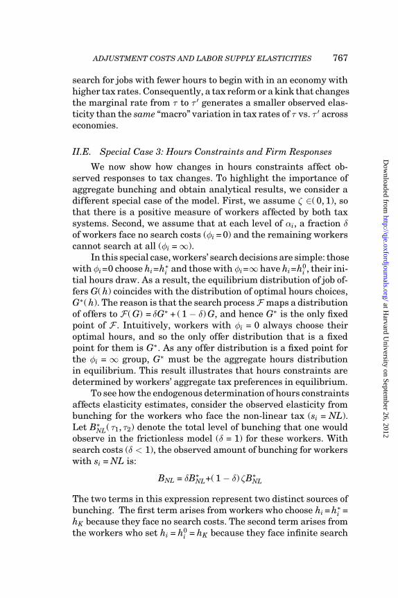
Toseehowtheendogenous determinationofhours constraintsaffects elasticity estimates, consider the observed elasticity frombunching for the workers who face the non-linear tax (si = NL).Let B∗NL(τ1, τ2) denote the total level of bunching that one wouldobserve in the frictionless model (δ = 1) for these workers. Withsearch costs (δ < 1), the observed amount of bunching for workerswith si = NL is:
BNL = δB∗NL+(1− δ)ζB∗NL
The twoterms in this expression represent twodistinct sources ofbunching. The first term arises from workers whochoose hi =h∗i =hK because they face nosearch costs. The secondterm arises fromthe workers who set hi = h0
i = hK because they face infinite search
at Harvard U
niversity on September 26, 2012
http://qje.oxfordjournals.org/D
ownloaded from
768 QUARTERLY JOURNAL OF ECONOMICS
costs. Because the aggregate distribution of hours coincides withthe optimal aggregate distribution, a fraction ζB∗NL of the equi-librium job offers have hours of hK . We label the first componentof bunching (BI
NL = δB∗NL) “individual bunching” because it arisesfrom individuals’ choices tolocate at the kink via jobsearch.15 Welabel the second component (BA
NL=(1− δ)ζB∗NL) “aggregate bunch-ing”becauseit arises fromtheaggregationof workers’ preferencesby either unions or firms.
The signature of aggregate bunching is that it generatesbunching even amongst workers who have no incentive to locateat the kink. Consider workers with si = L, who face a linear taxschedule and experience no change in marginal tax rates at hK .Because of the interaction of hours constraints with search costs,these workers also bunch at the kink via the aggregate bunchingchannel. These workers draw h0
i = hK with probability ζB∗NL andare forced to retain that offer if φi =∞. The amount of bunchingobserved for workers with si = L is therefore BL = (1 − δ)ζB∗NL =BA
NL. This equivalence between BL and BANL is useful empirically
because we cannot measure BANL directly (as we do not observe
search behavior), but we can measure BL since we do observeworkers’ tax schedules. Intuitively, any bunching among thosewho do not face a kink must represent aggregate bunching.
The observed elasticity from bunching for workers withsi = NL is:
ε =BNL(τ1, τ2)/g∗NL(hK)
K ln(
1−τ11−τ2
) = δε+(1− δ)ζε < ε
Theobservedelasticityis smallerthanthestructural elasticitybe-cause search costs prevent some workers who would like to be atthe kink from moving there.16 The observed elasticity rises with
15. A fraction (B∗NL)2 of workers with φi = 0 and h∗i = hK draw the h0i = hK to
begin with and are therefore indifferent between retaining h0i and searching for
their optimal job. To simplify notation, we classify these workers as “individualbunchers” by assuming that they choose to search for a new job.
16. In this special case, the total amount of bunching including all workers(both L and NL) equals the amount of bunching in the frictionless case (δ = 0) be-cause G(h)= G∗(h). However, the composition of those at the kink differs whenδ > 0: some of those who bunch face the linear tax. This is why ε < ε for work-ers of type NL. In the general model where workers face finite adjustment costs,G(h)/= G∗(h) and total bunching no longer coincides with that in the frictionlesscase.
at Harvard U
niversity on September 26, 2012
http://qje.oxfordjournals.org/D
ownloaded from

ADJUSTMENT COSTS AND LABOR SUPPLY ELASTICITIES 769
the scope of the kink ζ – the fraction of workers in the economywho face the non-linear tax schedule. When more workers facea change in tax incentives at an earnings level of K, firms arecompelled tooffer more jobs in equilibrium at hK hours tocater toaggregatepreferences. Thus a kinkthat affects moreworkers gen-erates more aggregate bunching BA
NL and thereby leads to moretotal bunching and a larger observed elasticity ε.
As the scope of the kink approaches ζ =1, BNL → B∗NL and ε→ε inthis special case. Conversely, as ζ approaches 0, BA
NL convergesto 0 because firms only cater to aggregate preferences. It followsthat the bunching observedat kinks that affect fewworkers in theeconomy constitutes a pure measure of individual bunching:
(11) limζ→0
BNL = BINL
This equivalence between limζ→0 BNL and BINL is also useful em-
pirically because we cannot directly observe BINL, but can observe
limζ→0 BNL by studying bunching at kinks that apply tofewwork-ers.17 These results lead to our second testable prediction.
PREDICTION 2: Search costs interact with hours constraints togenerate aggregate bunching. Aggregate bunching and theobserved elasticity rise with the fraction of workers who facethe kink:
BANL = BL > 0 iff ζ > 0(12)
∂BANL
∂ζ> 0 and
∂ε
∂ζ> 0.
The source of aggregate bunching is that the distribution ofjobs offeredin equilibrium reflects the aggregation of workers’ taxpreferences. Therefore, in occupations where workers are moretax elastic, one should observe a higher level of both individualand aggregate bunching. To see this, consider the Q-sector ex-tension of the model described above. The amount of individualbunching in occupation q is BI
NL,q = δζB∗NL,q and the amount of
aggregate bunching is BANL,q = (1− δ) ζB∗NL,q. As the structural
elasticity εq increases, the fraction of workers who would opti-mally locate at the kink (B∗NL,q) increases, increasing both BI
NL,q
17. This is why the bunching in special case 2 above (where ζ = 0) is drivenpurely by individual search behavior rather than aggregate responses.
at Harvard U
niversity on September 26, 2012
http://qje.oxfordjournals.org/D
ownloaded from

770 QUARTERLY JOURNAL OF ECONOMICS
and BANL,q because δ and ζ are constant.18 This leads to our third
and final prediction.
PREDICTION 3: The amount of aggregate bunching and individualbunching are positively correlated across occupations:
(13) cov(
BINL,q, BA
NL,q
)> 0
OnlineAppendixA presents analogs of predictions 2 and3 forobserved elasticities from tax reforms.
Micro vs. Macro Elasticities. The structural elasticity ε con-tinues todeterminethemacroelasticitywithfirmresponses. Con-sider again the two economies with different linear tax rates, τand τ ′, for workers of type si = L. But now assume that all work-ers face the linear tax (ζ = 0), so that firms respond to this taxvariation. The results above imply that the difference in equilib-rium hours across the twoeconomies coincides with the differencein optimal hours. It follows immediately that the difference inaverage hours of work between the two economies is
E loghi(τ′)−E loghi(τ) =E logh∗i (τ ′)−E logh∗i (τ) = ε∙( log τ ′−log τ)
Hence, theobservedmacroelasticityequals thestructural elastic-ity (εMAC=ε) even in the presence of coordinate responses totaxes.This result highlights a second reason that the macroeconomiceffects of taxes could be larger than microeconometric estimates.Variation in tax rates across economies shifts the aggregate dis-tribution of workers’ preferences and thereby induces changes inthe hours constraints set by firms. In contrast, tax reforms orkinks that affect a small subgroup of workers do not generatesubstantial changes in hours constraints.
We derived the three predictions in special cases because thegeneral model with finite search costs and endogenous hours con-straints is analytically intractable. In Chetty et al. (2009) we usenumerical simulations to verify that the three predictions hold inthe general case. The simulations also show that the macro elas-ticity is typically close to ε in the general model. We therefore pro-ceed to test the predictions empirically and determine the extent
18. If workers could switch between sectors, this correlation result would bereinforced because more elastic workers would sort toward sectors with moreaggregate bunching.
at Harvard U
niversity on September 26, 2012
http://qje.oxfordjournals.org/D
ownloaded from
ADJUSTMENT COSTS AND LABOR SUPPLY ELASTICITIES 771
to which adjustment costs and hours constraints attenuate microelasticity estimates in practice.
III. INSTITUTIONAL BACKGROUND AND DATA
The Danish labor market is characterized by a combinationof institutional regulation and flexibility, commonly termed “flex-icurity.” The vast majority of private sector jobs are covered bycollective bargaining agreements, negotiated by unions andemployer associations. The collective bargains set wages at theoccupationlevel as a functionof seniority, qualifications, degreeofresponsibility, etc. The contracts are typically negotiated atintervals of 2–4 years. Despite this relatively rigid bargainingstructure, rates of job turnover are relatively high and the un-employment rate is relatively low. For example, Andersen andSvarer (2007) report that rates of job creation and job destructionfor most sectors and the overall economy in Denmark are com-parable to those in the U.S. The unemployment rate in 2000 inDenmark was 5.4%, among the lowest in Europe.
During the period we study (1994–2001), income was taxedusing a three-bracket system. Figure IIa shows the tax schedulein 2000 in terms of Danish Kroner (DKr). Note that $1 ≈ DKr 6.Themarginal taxratebegins at approximately45%, referredtoasthe “bottom tax.”19 At an income of DKr 164,300, a “middle tax” islevied in addition tothe bottom tax. The net-of-tax wage rate fallsby 11% at the point where the middle bracket begins. Finally, atincomes aboveDKr267,600, individuals paythe“toptax”ontopofthe other taxes, bringing the marginal tax rate to approximately63%. The net-of-tax wage rate falls by 30% at the point where thetop bracket begins. Approximately 25% of wage earners pay thetop tax during the period we study. The large jump in marginaltax rates in a central part of the income distribution makes theDanish tax system particularly interesting for our purposes.20
Figure IIbplots themovement inthetopbracket cutoffacrossyears in real and nominal terms. Danish tax law stipulates that
19. Individuals with incomes below DKr 33,000 are exempt from this bottomtax; in practice, virtually all wage earners earn more than this threshold.
20. Denmark also has a complex transfer system that affects incentives forlowincomes (Kleven andKreiner 2006). We donot model the transfer system herebecausetransferprograms affect veryfewindividuals’ marginal incentives aroundthe middle and top tax cutoffs that are the focus of our empirical analysis.
at Harvard U
niversity on September 26, 2012
http://qje.oxfordjournals.org/D
ownloaded from

772 QUARTERLY JOURNAL OF ECONOMICS
FIGURE IIThe Danish Income Tax System
Panel (a) plots the marginal tax rate in 2000 vs. income for individuals livingin Copenhagen, including the national tax, regional tax, andmunicipal tax. Panel(b) plots the level of taxable income above which earners must pay the top bracketnational tax. The series in dark gray diamonds, plotted on the right y-axis, showsthenominal cutoff; theseries inlight graysquares, plottedontheleft y-axis, showsthe cutoff in real 2000 DKr.
at Harvard U
niversity on September 26, 2012
http://qje.oxfordjournals.org/D
ownloaded from

ADJUSTMENT COSTS AND LABOR SUPPLY ELASTICITIES 773
the movement in the top tax bracket from year t to year t + 1 is apre-determinedfunction of wage growth in the economy from yeart−2 toyear t−1 (two-year laggedwage growth). This mechanical,pre-determined movement of the cutoffs rules out potential con-cerns that the bracket cutoffs may be endogenously set as a func-tion of labor market contracts. Over the period of study, inflationwas between 1.8% and 2.9% per year. Because of the adjustmentrule, the top bracket cutoffdeclines in real terms from 1994–1997and then increases from 1998–2001.
In addition tothe variation in tax rates across brackets, therewere also some small tax reforms during the period we study.For example, in 1994 and 1995, there were two separate middletaxes that were consolidated into a single middle tax in subse-quent years. Starting in 1999, net capital losses could not be de-ductedfromthemiddletaxbaseandcontributions tocertaintypesof pensions could nolonger be deducted from the top tax base. Fi-nally, the middle and top tax bracket cutoffs change in real termsacross years. These tax reforms generate changes in net-of-taxrates between−10% to +10% for certain subgroups, yielding sev-eral tax changes of small size and scope.
There are two tax bases relevant for our analysis: one for thetop tax and one for the middle taxes. The top tax base dependsalmost entirely on individual income; the middle tax base is afunction of household income. We study behavior at the individ-ual level because our analysis focuses primarily on the top tax,but we account for joint aspects of the tax system when relevant(e.g. when studying the middle tax). We use the term “taxableincome” to refer to the tax base relevant to a particular tax; forinstance, when studying bunching around the top tax cutoff, weuse “taxable income” to refer to the top tax base.21 Wage earn-ings, self-employment income, transfer payments, and gifts areall subject to both the middle and top income taxes. Most pensioncontributions are tax deductible and the marginal dollar of capi-tal income is not subject tothe top tax for most individuals. Thesefeatures of the tax code create an incentive to shift earnings fromlaborincometocapital incomeandpensions. See MinistryofTaxa-tion(2002) foramorecomprehensivedescriptionof theDanishtaxsystem.
21. The Danish tax system includes a technical concept of “Taxable Income.”Our use of the term “taxable income” does not refer to that technical concept.
at Harvard U
niversity on September 26, 2012
http://qje.oxfordjournals.org/D
ownloaded from

774 QUARTERLY JOURNAL OF ECONOMICS
Data. We merge several administrative registers provided byStatistics Denmark. The primary dataset is the tax register from1994-2001, which contains panel data on wage earnings, self-employment income, pensions, capital income and deductions,spouse ID, andseveral other characteristics. The tax register con-tains records for more than 99.9% of individuals between the agesof 15–70 inthepopulation. Wemergethetaxdata withtheDanishIntegrated Database for Labor Market Research (IDA), whichincludes data on education, firm ID, occupation, labor market ex-perience, and number of children for every person in Denmark.Additional details onthedataset andvariabledefinitions aregivenin Online Appendix B.
Starting from the population dataset, we restrict attentionto individuals who (1) are between the ages of 15 and 70 and (2)are wage earners, excluding the self-employed and pensioners.22
These exclusions leave us with an analysis sample of 17.9 millionobservations of wage earners. Much of our analysis focuses on thesubset of 6.8 millionobservations forwageearners that fall within50,000 of the top tax cutoff. We also study the 1.8 million obser-vations of self-employed individuals separately.
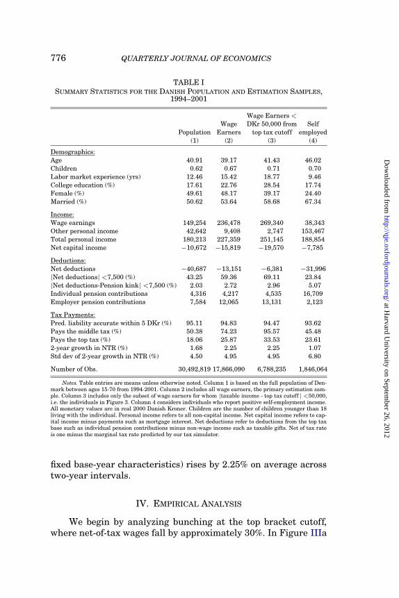
Table I presents summary statistics for the population of15–70 year olds as a whole, all wage earners, the subset of wageearners withinDKr50,000 of thetoptaxcutoff, andself-employedindividuals. Themeanindividual personal (non-capital) incomeinthe population is DKr 180,213 ($30,000) for the populationand DKr 227,359 ($38,000) for wage earners. Mean net capitalincome is negative because mortgage interest payments exceedcapital income for most individuals. We define “net deductions”asdeductions minus non-wageincome(accountingforspousal deduc-tions), orequivalently, wageearnings minus taxableincome. Mostwageearners havesmall net deductions (60% havedeductions lessthan DKr 7,500 in magnitude), a fact that proves useful for ourempirical analysis. The mean level of net deductions is negativebecause some individuals have substantial non-wage income.
We construct a tax simulator that calculates tax liabilitiesand marginal tax rates using these data. Given our focus on thetop tax base, we compute marginal tax rates for individuals (i.e.,
22. The endogenous sample selection induced by dropping the self-employeddoes not spuriously generate bunching. There is significant bunching in the wageearnings distribution even in the full population: b = 0.73 in the full population vs.b = 0.71 for the subgroup of wage earners reported in Figure IIIa below.
at Harvard U
niversity on September 26, 2012
http://qje.oxfordjournals.org/D
ownloaded from
ADJUSTMENT COSTS AND LABOR SUPPLY ELASTICITIES 775
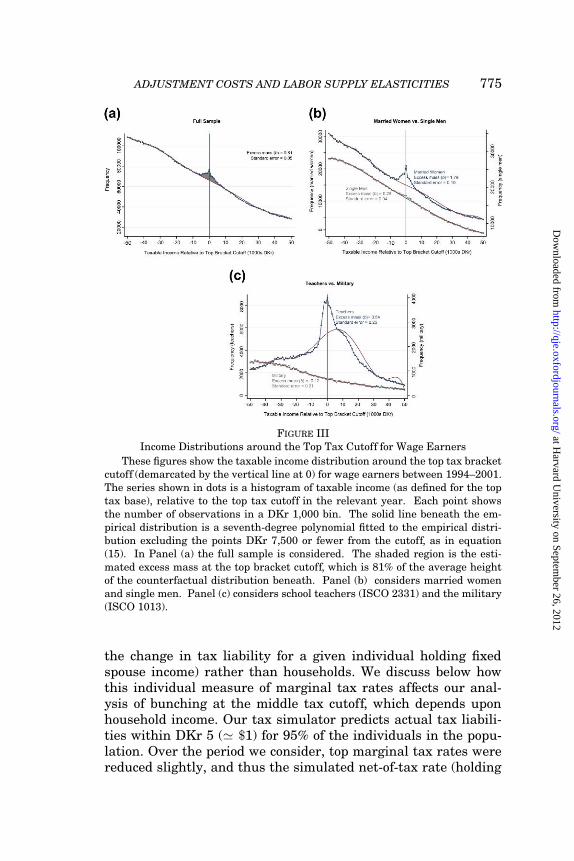
FIGURE IIIIncome Distributions around the Top Tax Cutoff for Wage Earners
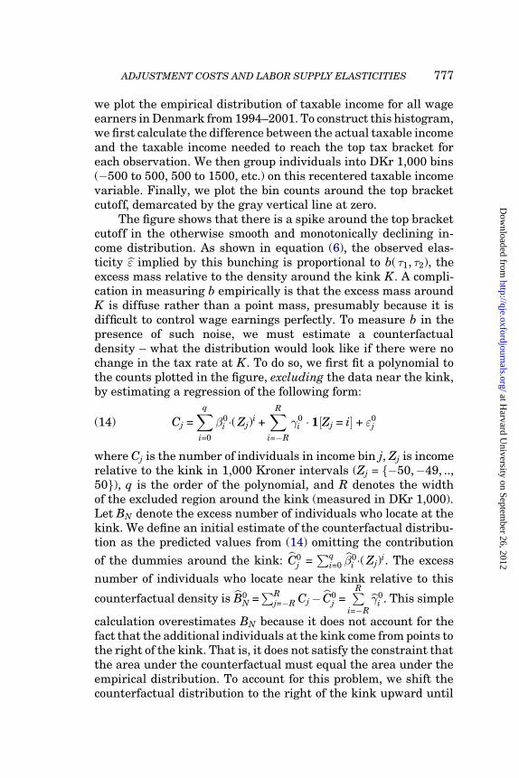
These figures showthe taxable income distribution around the top tax bracketcutoff (demarcated by the vertical line at 0) for wage earners between 1994–2001.The series shown in dots is a histogram of taxable income (as defined for the toptax base), relative to the top tax cutoff in the relevant year. Each point showsthe number of observations in a DKr 1,000 bin. The solid line beneath the em-pirical distribution is a seventh-degree polynomial fitted to the empirical distri-bution excluding the points DKr 7,500 or fewer from the cutoff, as in equation(15). In Panel (a) the full sample is considered. The shaded region is the esti-mated excess mass at the top bracket cutoff, which is 81% of the average heightof the counterfactual distribution beneath. Panel (b) considers married womenand single men. Panel (c) considers school teachers (ISCO 2331) and the military(ISCO 1013).
the change in tax liability for a given individual holding fixedspouse income) rather than households. We discuss below howthis individual measure of marginal tax rates affects our anal-ysis of bunching at the middle tax cutoff, which depends uponhousehold income. Our tax simulator predicts actual tax liabili-ties within DKr 5 (' $1) for 95% of the individuals in the popu-lation. Over the period we consider, top marginal tax rates werereduced slightly, and thus the simulated net-of-tax rate (holding
at Harvard U
niversity on September 26, 2012
http://qje.oxfordjournals.org/D
ownloaded from
776 QUARTERLY JOURNAL OF ECONOMICS
TABLE ISUMMARY STATISTICS FOR THE DANISH POPULATION AND ESTIMATION SAMPLES,
1994–2001
Wage Earners<Wage DKr 50,000 from Self
Population Earners top tax cutoff employed(1) (2) (3) (4)
Demographics:Age 40.91 39.17 41.43 46.02Children 0.62 0.67 0.71 0.70Labor market experience (yrs) 12.46 15.42 18.77 9.46College education (%) 17.61 22.76 28.54 17.74Female (%) 49.61 48.17 39.17 24.40Married (%) 50.62 53.64 58.68 67.34
Income:Wage earnings 149,254 236,478 269,340 38,343Other personal income 42,642 9,408 2,747 153,467Total personal income 180,213 227,359 251,145 188,854Net capital income −10,672 −15,819 −19,570 −7,785
Deductions:Net deductions −40,687 −13,151 −6,381 −31,996|Net deductions| <7,500 (%) 43.25 59.36 69.11 23.84|Net deductions-Pension kink| <7,500 (%) 2.03 2.72 2.96 5.07Individual pension contributions 4,316 4,217 4,535 16,709Employer pension contributions 7,584 12,065 13,131 2,123
Tax Payments:Pred. liability accurate within 5 DKr (%) 95.11 94.83 94.47 93.62Pays the middle tax (%) 50.38 74.23 95.57 45.48Pays the top tax (%) 18.06 25.87 33.53 23.612-year growth in NTR (%) 1.68 2.25 2.25 1.07Std dev of 2-year growth in NTR (%) 4.50 4.95 4.95 6.80
Number of Obs. 30,492,819 17,866,090 6,788,235 1,846,064
Notes. Table entries are means unless otherwise noted. Column 1 is based on the full population of Den-mark between ages 15-70 from 1994-2001. Column 2 includes all wage earners, the primary estimation sam-ple. Column 3 includes only the subset of wage earners for whom |taxable income - top tax cutoff | <50,000,i.e. the individuals in Figure 3. Column 4 considers individuals who report positive self-employment income.All monetary values are in real 2000 Danish Kroner. Children are the number of children younger than 18living with the individual. Personal income refers to all non-capital income. Net capital income refers to cap-ital income minus payments such as mortgage interest. Net deductions refer to deductions from the top taxbase such as individual pension contributions minus non-wage income such as taxable gifts. Net of tax rateis one minus the marginal tax rate predicted by our tax simulator.
fixed base-year characteristics) rises by 2.25% on average acrosstwo-year intervals.
IV. EMPIRICAL ANALYSIS
We begin by analyzing bunching at the top bracket cutoff,where net-of-tax wages fall by approximately 30%. In Figure IIIa
at Harvard U
niversity on September 26, 2012
http://qje.oxfordjournals.org/D
ownloaded from
ADJUSTMENT COSTS AND LABOR SUPPLY ELASTICITIES 777
we plot the empirical distribution of taxable income for all wageearners inDenmarkfrom1994–2001. Toconstruct this histogram,wefirst calculatethedifferencebetweentheactual taxableincomeand the taxable income needed to reach the top tax bracket foreach observation. We then group individuals into DKr 1,000 bins(−500 to 500, 500 to 1500, etc.) on this recentered taxable incomevariable. Finally, we plot the bin counts around the top bracketcutoff, demarcated by the gray vertical line at zero.
The figure shows that there is a spike around the top bracketcutoff in the otherwise smooth and monotonically declining in-come distribution. As shown in equation (6), the observed elas-ticity ε implied by this bunching is proportional to b(τ1, τ2), theexcess mass relative to the density around the kink K. A compli-cation in measuring b empirically is that the excess mass aroundK is diffuse rather than a point mass, presumably because it isdifficult to control wage earnings perfectly. To measure b in thepresence of such noise, we must estimate a counterfactualdensity – what the distribution would look like if there were nochange in the tax rate at K. To do so, we first fit a polynomial tothe counts plotted in the figure, excluding the data near the kink,by estimating a regression of the following form:
(14) Cj =q∑
i=0
β0i ∙(Zj)
i +R∑
i=−R
γ0i ∙ 1[Zj = i] + ε0
j
where Cj is the number of individuals in income bin j, Zj is incomerelative to the kink in 1,000 Kroner intervals (Zj = {−50,−49, ..,50}), q is the order of the polynomial, and R denotes the widthof the excluded region around the kink (measured in DKr 1,000).Let BN denote the excess number of individuals who locate at thekink. We define an initial estimate of the counterfactual distribu-tion as the predicted values from (14) omitting the contribution
of the dummies around the kink: C0j =
∑qi=0 β
0i ∙(Zj)i. The excess
number of individuals who locate near the kink relative to this
counterfactual density is B0N =∑R
j=−R Cj− C0j =
R∑
i=−Rγ0
i . This simple
calculation overestimates BN because it does not account for thefact that theadditional individuals at thekinkcomefrompoints totheright of thekink. That is, it does not satisfytheconstraint thatthe area under the counterfactual must equal the area under theempirical distribution. To account for this problem, we shift thecounterfactual distribution to the right of the kink upward until
at Harvard U
niversity on September 26, 2012
http://qje.oxfordjournals.org/D
ownloaded from

778 QUARTERLY JOURNAL OF ECONOMICS
it satisfies the integration constraint. In particular, we define thecounterfactual distribution Cj = βi∙(Zj)i as the fitted values fromthe regression
(15) Cj∙(1 + 1[j > R]BN∑∞
j=R+1 Cj)=
q∑
i=0
βi∙(Zj)i +
R∑
i=−R
γi ∙ 1[Zj = i] + εj
where BN =∑R
j=−R Cj − Cj =R∑
i=−Rγi is the excess number of indi-
viduals at the kink implied by this counterfactual.23 Finally, wedefine our empirical estimate of b as the excess mass around thekinkrelativetotheaveragedensityof thecounterfactual earningsdistribution between−R and R:
(16) b =BN
∑Rj=−R Cj/(2R + 1)
Thesolidcurveinthefigureshows thecounterfactual density {Cj}predicted using this procedure with a seventh-degree polynomial(q = 7) and a window of DKr 15,000 centered around the kink(R = 7). Theshadedregionshowstheestimatedexcessmassaroundthekink. Withtheseparameters, weestimate b = 0.81 – theexcessmass around the kink is 81% of the average height of the counter-factual distribution within DKr 7,500 of the kink. The qualitativeresults we report below are not sensitive to changes in q and Ror the way in which we correct the counterfactual to satisfy theintegration constraint. The reason is that the differences we doc-ument in observed elasticities are much larger than the changesinduced by varying the specification of the counterfactual.
We calculate a standard error for b using a parametric boot-strapprocedure. We drawfrom the estimatedvector of errors ξj in(15) with replacement to generate a new set of counts and applythe technique above tocalculate a newestimate bk. We define thestandarderror of b as the standarddeviation of the distribution ofbks. Since we observe the exact population distribution of taxableincome, this standarderrorreflects errorduetomisspecificationofthe polynomial for the counterfactual income distribution rather
23. Because BN is a function of βi, the dependent variable in this regressiondepends upon the estimates of βi. We therefore estimate (15) by iteration, recom-puting BN using the estimated βi until we reach a fixed point. The bootstrappedstandarderrors that wereport belowadjust forthis iterativeestimationprocedure.
at Harvard U
niversity on September 26, 2012
http://qje.oxfordjournals.org/D
ownloaded from
ADJUSTMENT COSTS AND LABOR SUPPLY ELASTICITIES 779
than sampling error. The standard error associated with our esti-mate of b is 0.05. The null hypothesis that there is noexcess massat the kink relative to the counterfactual distribution is rejectedwith a t-statistic of 17.6, implying p < 1× 10⁻⁹.
There is substantial heterogeneity across groups in theamount of bunching. Figure IIIb shows that excess mass at thekink is much larger for married women (b = 1.79) than for sin-gle men (b = 0.25), consistent with existing evidence that marriedwomen exhibit the highest labor supply elasticities.24 Figure IIIcshows that there is also substantial heterogeneity across occu-pations: teachers exhibit substantial bunching around the kink(b = 3.54), whereas the military does not (b = −0.12, statisticallyinsignificant).25 We return to explore the sources of this hetero-geneity in Section IV.B below.
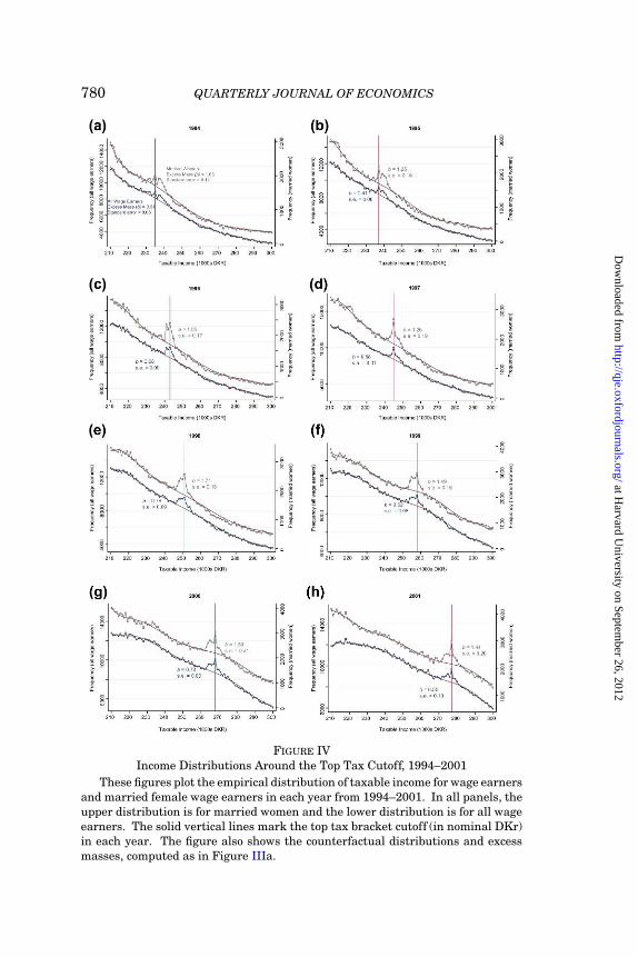
The identification assumption underlying causal inferenceabout the effect of taxes on earnings in the preceding analysisis that the income distribution would be smooth if there were nojump in tax rates at the location of the top bracket cutoff. Thisidentification assumption can be relaxed by exploiting the move-ment in the topbracket cutoffacross years. Figure IV displays thedistribution of taxable income in each year from 1994–2001 for allwage earners and for married women. The excess mass for bothgroups follows themovement inthetopbracket cutoffveryclosely.In Figure V, we investigate whether the excess mass tracks taxchanges, inflation, oraveragewagegrowthovertime. Weconsiderthe periodfrom 1997 to2001, during which the toptax cutoffrisesin real terms. Noting that the excess mass is located at the toptax cutoff in 1997, the figure shows three possibilities for its loca-tion in 2001: the 2001 top tax cutoff, the 1997 cutoff adjusted forinflation, andthe 1997 cutoffadjustedfor average wage growth inthe economy. In both the full population of wage earners and thesubgroupof marriedwomen, the excess mass that was at the 1997kink clearly moves to the 2001 kink rather than following infla-tionoraveragewagegrowth. Thesamepatternis observedduringotherperiods whenthetoptaxcutoffis declininginreal terms (see
24. Inprinciple, thebunchingformarriedwomencouldbeexaggeratedbywagepayments from self-employed husbands seeking to reduce their tax liabilities. Inpractice, we find that the amount of bunching is virtually unchanged when weexclude households with at least one self-employed person from the sample.
25. Approximately 50% of wage earners in Denmark work in the publicsector.We find slightly more bunching for those employed in the private sector (b = 0.67)than those in the public sector (b = 0.5).
at Harvard U
niversity on September 26, 2012
http://qje.oxfordjournals.org/D
ownloaded from
780 QUARTERLY JOURNAL OF ECONOMICS
FIGURE IVIncome Distributions Around the Top Tax Cutoff, 1994–2001
Thesefigures plot theempirical distributionof taxableincomeforwageearnersand married female wage earners in each year from 1994–2001. In all panels, theupper distribution is for married women and the lower distribution is for all wageearners. The solid vertical lines mark the top tax bracket cutoff (in nominal DKr)in each year. The figure also shows the counterfactual distributions and excessmasses, computed as in Figure IIIa.
at Harvard U
niversity on September 26, 2012
http://qje.oxfordjournals.org/D
ownloaded from
ADJUSTMENT COSTS AND LABOR SUPPLY ELASTICITIES 781
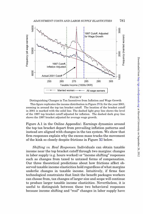
FIGURE VDistinguishing Changes in Tax Incentives from Inflation and Wage Growth
This figure replicates the income distribution in Figure IV(h) for the year 2001,zooming in around the top tax bracket cutoff. The location of the bracket cutoffin 2001 is marked with the solid line. The dashed light gray line shows the levelof the 1997 top bracket cutoff adjusted for inflation. The dashed dark gray lineshows the 1997 bracket adjusted for average wage growth.
Figure A.1 in the Online Appendix). Earnings dynamics aroundthe top tax bracket depart from prevailing inflation patterns andinstead are aligned with changes in the tax system. We showthatfirm responses explain why the excess mass tracks the movementof the kink so closely despite frictions in Figure XI below.
Shifting vs. Real Responses. Individuals can obtain taxableincome near the top bracket cutoff through two margins: changesin labor supply (e.g. hours worked) or “income shifting” responsessuch as changes from taxed to untaxed forms of compensation.Our three theoretical predictions about how frictions affect ob-servedtaxableincomeelasticities holdregardless ofwhat marginsunderlie changes in taxable income. Intuitively, if firms facetechnological constraints that limit the benefit packages workerscan choose from, tax changes of largersize andscope will continueto produce larger taxable income elasticities. Nevertheless, it isuseful to distinguish between these two behavioral responsesbecause income shifting and “real” changes in labor supply have
at Harvard U
niversity on September 26, 2012
http://qje.oxfordjournals.org/D
ownloaded from

782 QUARTERLY JOURNAL OF ECONOMICS
different normative implications (Slemrod and Yitzhaki 2002;Chetty 2009).
Therearetwochannels throughwhichindividuals canchangetheirreportedtaxable incomewithout changinglaborsupply: eva-sion and avoidance. Kleven et al. (2010) study audited Danish taxrecords and find that there is virtually no tax evasion in wageearnings because of third-party reporting by firms. We find thatthereis substantial bunching(b = 0.68) eveninwageearnings (seeFigure A.2). We therefore conclude that the bunching we observeis not driven by evasion.
The second and more important income shifting channel islegal tax avoidance. The simplest method of reducing current taxliabilities is to contribute to tax-deductible pension accounts. Weinvestigate the extent of such shifting by adding employer andemployee pension contributions back to taxable income. We findthat thedistributionof this broadermeasureof compensationstillexhibits substantial bunching relative to the statutory top taxbracket cutoff that would apply to individuals with zero pensioncontributions, rejecting the hypothesis that all of the bunchingobserved in taxable income is driven by shifts to pensions (seeFigure A.2).We conclude that pension shifting is responsible foronlya small amount of thebunchingintaxable incomeweobserveat the toptax cutoff. The relatively small amount of pension shift-ing is likely driven by the generosity of Denmark’s social securityprograms. An analogous exercise shows that shifting into capitalincome, which is untaxed in the top tax base, is responsible forvirtually none of the bunching at the top kink.
Although the behavioral responses at the toptax cutoffdonotappear to be driven by any observable method of income shifting,we cannot rule out the possibility that individuals shift theircompensation to unobservable nontaxable compensation to avoidpaying the top income tax. For example, we cannot detect substi-tution of compensation from wage earnings into office amenitieswhen individuals cross into the top tax bracket. We also cannotrule out intertemporal shifting of wage earnings to avoid payingthe top tax. The only way to definitively rule out such responsesis to examine changes in hours worked directly. Unfortunately,our dataset does not contain information on hours of work. Never-theless, we believe that most of the observed bunching in taxableincome reflects “real” distortions in behavior that have efficiencycosts. Few salaried workers at the 75th percentile of the incomedistribution have the ability to shift income into other forms of
at Harvard U
niversity on September 26, 2012
http://qje.oxfordjournals.org/D
ownloaded from

ADJUSTMENT COSTS AND LABOR SUPPLY ELASTICITIES 783
FIGURE VIIncome Distributions around the Middle Tax Cutoff
Panels (a) and (c) plot the empirical distributions of taxable income (as de-fined for the middle tax base) around the middle tax cutoff, where net-of-tax wagerates fall by approximately 10%. Panel (b) plots the distribution of wage earningsaround the middle and top tax cutoffs. Panels (a) and (b) include all wage earn-ers, while panel (c) includes only married female wage earners. All panels showcounterfactual distributions and excess masses, computed as in Figure IIIa. Eachpanel alsoreports theamount of bunchingpredictedif theelasticitywerethesameas that estimated from the amount of bunching at the top bracket cutoff for thecorresponding income measure and subgroup.
compensationoracross time(Slemrod1995; Goolsbee2000). More-over, even if compensation is distorted toward office amenities in-stead of wages, the marginal efficiency cost of such distortionsequals the marginal efficiency cost of changes in hours of work(Feldstein 1999).
IV.A. Prediction 1: Size of Tax Changes
We now test the first prediction by comparing the amountof bunching at the top tax kink with bunching at smaller kinksand observed elasticities from small tax reforms. Figure VI
at Harvard U
niversity on September 26, 2012
http://qje.oxfordjournals.org/D
ownloaded from

784 QUARTERLY JOURNAL OF ECONOMICS
shows the distributions of taxable income around the middle taxcutoff, where the net-of-tax rate falls by approximately 10%.26
FigureVIa shows that thereis virtuallynobunchingat themiddletax cutoff (b = 0.06) in taxable income for the full population ofwage earners. Moreover, the estimated excess mass at the mid-dle tax converges to zero as the degree of the polynomial is in-creased, whereas the estimated excess mass at the top kink is notsensitive to the degree of the polynomial. Because the definitionsof “taxable income” differ for the top and middle tax bases, Fig-ureVIbplots thedistributionof wageearnings aroundbothkinks.Consistent with Figure VIa, there is significantly more bunchingat the top kink than the middle kink in wage earnings. FigureVIc shows that the amount of bunching remains small and sta-tistically insignificant even for the subsample of married women,who exhibit substantial bunching at the top kink as shown inFigure IIIb.
Note that smaller kinks should generate less bunching evenin the frictionless model, simply because the change in incentivesis smaller. We therefore compare the excess mass at these smallerkinks with the amount of excess mass that would be generated ifthe elasticity were the same as that implied by the excess massat the large top tax kink. In all cases, the amount of bunchingobserved in the empirical distribution at the middle kink is sig-nificantly less than what would be predicted by the frictionlessmodel. For example, the frictionless model predicts b = 0.16 atthe middle kink for all wage earners (Figure VIa). The null hy-pothesis that the predicted excess mass equals the actual excessmass at the middle kink can be rejected with p < 0.01.
Next, we estimate observed elasticities using changes inmarginal rates by legislated reforms. As described in Section III,several small tax reforms in Denmark between 1994 and 2001created changes in net-of-tax rates of between −10% and +10%.These reforms generate differential changes in net-of-tax ratesacross income groups, motivating a difference-in-differenceresearch design. Let Δ log yi,t = log yi,t − log yi,t−2 denote the logchangeinwageearnings fromperiod t−2 tot andΔ log(1−MTRi,t)the log change in net-of-tax rates over the same period. Follow-ing Gruber and Saez (2002), we estimate the following regression
26. In 1994 and 1995, the tax system includes an additional “upper middletax.” Figure VI only considers the lower middle tax in these years, but there is nobunching at the upper middle tax cutoff either.
at Harvard U
niversity on September 26, 2012
http://qje.oxfordjournals.org/D
ownloaded from
ADJUSTMENT COSTS AND LABOR SUPPLY ELASTICITIES 785
specification using two-stage-least-squares:
(17) Δ log yi,t = α + βΔ log(1−MTRi,t) + f (yi,t−2) + γXi,t−2 + εi,t,
instrumenting for Δ log(1 −MTRi,t) with Δ log(1 −MTRsimi,t ), the
simulated change in net-of-tax rates holding the individual’s in-come and other characteristics fixed at their year t−2 levels. Thefunction f (yi,t−2) is a10-piecelinearsplineinbaseyearwageearn-ings andthevector Xi,t−2 is a set of baseyearcontrols that wevaryacross specifications. First-stage regressions of Δ log(1−MTRi,t)onΔ log(1−MTRsim
i,t ) have coefficients of approximately 0.6 witht-statistics exceeding 600.
Table II reports TSLS estimates from several variants of (17).In column (1), we estimate (17) on the full population of wageearners with the following controls: the 10-piece wage earningsspline, a 10-piece spline in total personal income andage andyearfixed effects. The estimated elasticity ε is very close to 0, and theupper bound of the 95% CI is ε = 0.004. Column (2) adds a 10-piece capital income spline, gender and marital status dummies,and occupation and region fixed effects as controls. The estimatedelasticity remains very close to zero, showing that the estimatesare robust to the set of covariates used to predict income growth.Column (3) considers the subgroup of married women using thebaseline specification in column (1). The observed elasticity in re-sponse to small tax changes remains near 0 for married womendespitethefact that theyexhibit substantial bunchingat thelargetop tax kink, as shown in Figure IIIb. In column (4), we furtherrestrict the sample to married women who are professionals andhaveabove-median(morethan19 years) labormarket experience.This subgroup also does not react significantly to small tax re-forms, yet it exhibits substantial bunchingat thetopkink(b=4.50,implying ε = 0.06).
Insum, ouranalysis confirms that largertaxchanges producelargerobservedelasticities. However, theelasticity impliedbythefrictionless model remains very small even at the largest kink.The observed elasticity from bunching at the 30% kink is ε ' 0.01for all wage earners and ε ' 0.02 for married women. We believethat these elasticity estimates remain substantially attenuatedrelative toε because the utility loss from ignoring the 30% changeintaxrates at thetopkinkis onlyaround2% ofconsumptiongivena structural elasticity of ε = 0.5 (Chetty 2011).
at Harvard U
niversity on September 26, 2012
http://qje.oxfordjournals.org/D
ownloaded from

786 QUARTERLY JOURNAL OF ECONOMICST
AB
LE
IIO
BS
ER
VE
DE
LA
ST
ICIT
YE
ST
IMA
TE
SU
SIN
GS
MA
LL
TA
XR
EF
OR
MS
Dep
end
ent
Va
ria
ble:
Log
Ch
an
gein
Wa
geE
arn
ings
Hig
h-E
xper
ien
ceW
age
Wag
eM
arri
edM
arri
edF
emal
eE
arn
ers
Ear
ner
sS
ubg
rou
p:
All
Wag
eE
arn
ers
Fem
ales
Pro
fess
ion
als
100-
300K
>20
0K
(1)
(2)
(3)
(4)
(5)
(6)
Log
chan
gein
net
-of-
tax
−0.
001
−0.
004
0.00
60.
000
−0.
006
−0.
001
rate
(Δlo
g(1
–t))
(0.0
03)
(0.0
03)
(0.0
05)
(0.0
11)
(0.0
03)
(0.0
03)
Ear
nin
gs×Δ
log
(1–t
)0.
005
(0.0
08)
Lab
orin
com
esp
lin
ex
xx
xx
x
Per
son
alin
com
esp
lin
ex
xx
xx
x
Yea
rfi
xed
effe
cts
xx
xx
xx
Age
fixe
def
fect
sx
xx
xx
x
Reg
ion
fixe
def
fect
sx
x
Occ
up
atio
nfi
xed
effe
cts
xx
Cap
ital
inco
me
spli
ne
xx
Gen
der
,Mar
ital
stat
us
xx
Obs
erva
tion
s11
,682
,651
8,30
2,90
53,
203,
515
159,
661
7,96
7,16
97,
585,
011
Not
es.
Sta
nd
ard
erro
rscl
ust
ered
byin
div
idu
alre
por
ted
inp
aren
thes
es.
Dep
end
ent
vari
able
inal
lsp
ecifi
cati
ons
istw
o-ye
argr
owth
rate
inre
alw
age
earn
ings
.In
dep
end
ent
vari
able
ofin
tere
stis
two-
year
grow
thra
tein
net
-of-
tax
rate
,in
stru
men
ted
usi
ng
two-
year
grow
thra
tein
sim
ula
ted
net
-of-
tax
rate
usi
ng
base
-yea
rva
riab
les.
Coe
ffici
ents
rep
orte
dca
nbe
inte
rpre
ted
asob
serv
edw
age
earn
ings
elas
tici
ties
from
tax
refo
rms.
All
spec
ifica
tion
sin
clu
de
10-p
iece
wag
eea
rnin
gsan
dto
tal
per
son
alin
com
esp
lin
esas
wel
las
age
and
year
fixe
def
fect
s.C
olu
mn
2al
soin
clu
des
a10
-pie
ceca
pit
alin
com
esp
lin
e,ge
nd
eran
dm
arit
alst
atu
sin
dic
ator
s,an
dre
gion
and
occu
pat
ion
fixe
def
fect
s.O
ccu
pat
ion
fixe
def
fect
sar
eav
aila
ble
only
for
asu
bset
ofye
ars
and
obse
rvat
ion
s.C
olu
mn
4re
stri
cts
atte
nti
onto
mar
ried
fem
ale
pro
fess
ion
als
wit
hm
ore
than
19ye
ars
ofla
bor
mar
ket
exp
erie
nce
.C
olu
mn
5in
tera
cts
the
log
chan
gein
net
ofta
xra
tew
ith
the
dif
fere
nce
betw
een
wag
eea
rnin
gsan
dth
eto
pta
xcu
toff
(mea
sure
din
DK
r10
0,00
0)to
test
wh
eth
erth
eta
xabl
ein
com
eel
asti
city
vari
esby
inco
me
leve
l.T
his
spec
ifica
tion
rest
rict
sth
esa
mp
leto
ind
ivid
ual
sw
ith
wag
eea
rnin
gsin
the
base
year
betw
een
DK
r10
0,00
0an
d30
0,00
0.C
olu
mn
6co
nsi
der
sin
div
idu
als
wit
hm
ore
than
DK
r20
0,00
0of
wag
eea
rnin
gsin
the
base
year
.
at Harvard U
niversity on September 26, 2012
http://qje.oxfordjournals.org/D
ownloaded from
ADJUSTMENT COSTS AND LABOR SUPPLY ELASTICITIES 787
Search Costs vs. Non-Constant Elasticities. If ε(τ , z) varieswith τ or z, the evidence that larger tax changes generate largerobserved elasticities could potentially be explained by variationin ε rather than adjustment costs. In our application, the middlekinks are at incomes of DKr 130,000–177,900, while the topkinksare at incomes of DKr 234,900–276,900. If higher income individ-uals are more elastic, one would observe more bunching at thetop kink even without frictions. We distinguish this explanationof our findings from frictions using three approaches.
First, we test whether taxable income elasticities differ byincome by interacting Δ log(1 − MTRi,t) with yi,t−2 (re-centeredaround the top tax cutoff). Column (5) of Table II shows that thisinteraction effect is small and insignificant (p = 0.52), indicatingthat there is no significant heterogeneity in observed elasticitiesby income. As an alternative approach to assessing heterogene-ity, we replicate the baseline specification in column (1) restrict-ing the sample to individuals with wage earnings exceeding DKr200,000. Column (6) shows that the estimated elasticity remainsvery close to zero, confirming that small tax changes do not gen-erate significant behavioral responses even for individuals facingthe top tax.
Second, we examine how the degree of bunching changes asthe middle and top tax cutoffs move across years. In the latteryears of our sample, the middle tax cutoff is higher in the incomedistribution, but the amount of bunching remains near zero (notshown). In contrast, bunching at the topkink remains substantialin all years (Figure IV).
As a third test of whether preference heterogeneity drivesthe differential bunching at the middle and top kinks, we focuson a subset of individuals whose incomes place them within DKr50, 000 of the topkink in year t andwithin DKr 50, 000 of the mid-dle kink in year t + 2. By studying these “switchers,” we can effec-tively remove individual fixed effects when comparing responsestothe middle and top kinks. We find that when near the top kink,these switchers exhibit substantial bunching (b = 0.54). However,just two years later, the same individuals show no excess propen-sity tobunch at the middle kink (b=0.06) despite having earningsnear that kink (see Figure A.3). The opposite pattern is observedforthosemovingfromthemiddletothetopkink. Weconcludethatvariation in observed elasticities is unlikely to explain the posi-tive relationship between larger tax changes and larger observedelasticities.
at Harvard U
niversity on September 26, 2012
http://qje.oxfordjournals.org/D
ownloaded from

788 QUARTERLY JOURNAL OF ECONOMICS
Jointness of the Middle Tax Cutoff. As notedabove, theDanishtax system has more elements of jointness at the middle kinkthan the top kink. In particular, spouses can transfer deductionsbetween each other to minimize their middle tax liabilities, ef-fectively making the middle tax a function of household income.Our individual-based measure of bunching at the middle tax isaccurate if individuals make wage earnings decisions based ontheir own tax liabilities. However, our method could in princi-ple understate the amount of bunching at the middle tax cutoffif spouses choose their earnings levels to minimize the tax bur-dens of the household as a whole rather than their own liability.As we explain in Online Appendix B, our method of computingbunching effectively computes the higher earner’s distance to thekink based on the joint tax liability of the household rather thantheindividual. Wefindthat bunchingat thetoptaxcutoffremainssignificantly larger than at the middle tax cutoff for the subsam-ple of individuals who are either the higher earner in a couple orare single (see Figure A.4). This result confirms that the differ-ences in observed elasticities at the top and middle kinks shownin Figures III and IV are robust to the way in which we accountfor the jointness of the middle kink.27
Perceptions of the Middle vs. Top Cutoffs. What are the coststhat workers face in responding to tax incentives? One possibilityis thecost of payingattentiontotaxes (e.g. ChettyandSaez 2009).FigureA.5 reports thedistributionof perceivedmiddleandtoptaxcutoff obtained from an internet survey of 3,299 individuals whowere members of a union representing publicand financial sectoremployees (FTF-A).28 The figure shows that knowledge of the toptax cutoff is better than the middle tax cutoff. The same qualita-tive pattern is exhibited across all education levels and occupa-tions in the sample. These survey responses must be viewed asanecdotal evidence because the survey was administered only tomembers of FTF-A and because the response rate is low (11%).Nevertheless, this evidence is consistent with our finding that
27. A furtherconcernis that it theremaybedifferences inthecosts ofbunchingat joint vs. individual kinks. For instance, jointness may allow the spouse withlower adjustment costs (e.g. the secondary earner) to choose a job that places thehousehold at the kink. Such effects would work against finding more bunching atthe top kink than the middle kink.
28. We thank Anders Frederikssen for making these data availableto us.
at Harvard U
niversity on September 26, 2012
http://qje.oxfordjournals.org/D
ownloaded from

ADJUSTMENT COSTS AND LABOR SUPPLY ELASTICITIES 789
observed elasticities are larger at the top kink than the middlekink.
IV.B. Prediction 2: Aggregate Bunching and Scope of Tax Changes
Totest thesecondprediction, webeginbyidentifyinga sourceof variation in the scope of kinks – the fraction of workers in theeconomy who face a given kink in the tax system. Recall thattaxable income is the sum of wage earnings and non-wage in-come minus deductions. Deductions consist primarily of pensioncontributions. Non-wage income includes items such as alimonyreceipts, stipends, and unemployment benefits. Because of het-erogeneity in non-wage income and deductions, the wage earn-ings required to reach the middle and top brackets vary acrossindividuals.
Approximately 60% of wage earners have net deductions(deductions minus non-wage income) less than DKr 7, 500 inmagnitude (see Figure A.6). This is because most individuals inDenmark make no tax deductible pension contributions and earnonly wage income. Thus, most individuals cross into the top taxbracket when their wage earnings exceed the top tax cutoff thatapplies to taxable income, which we term the “statutory” top taxcutoff. The distribution of deductions for the remaining 40% ofindividuals is diffuse, with one important exception. There is amass point inthedistributionof deductions at approximatelyDKr33, 000, which is driven by a cap on tax-deductible pension contri-butions. Individuals who make pensions contributions up the cap(approximately 2.7% of wage earners) reach the top tax bracketonly when their wage earnings exceed the statutory top tax cutoffby DKr 33, 000.
In this setting, the second prediction of our model consists ofthree parts: we should observe (1) significant aggregate bunchingat the statutory top tax kink that applies to 60% of workers, (2)little aggregate bunching at the “pension kink” that applies to2.7% of workers, and(3) more bunching for individuals with smalldeductions, as they have more common tax preferences. To testthese hypotheses, we study wage earnings distributions at theoccupation level because most wages are set through collectivebargains at the occupation level in Denmark.
Aggregate bunching is easiest to see through case studiesof occupations. Consider school teachers, who constituteapproximately 3% of wage earners in Denmark and form one of
at Harvard U
niversity on September 26, 2012
http://qje.oxfordjournals.org/D
ownloaded from

790 QUARTERLY JOURNAL OF ECONOMICS
FIGURE VIITeachers’ Wage Earnings Distributions
These two figures plot the empirical distribution of wage earnings around thestatutorytoptaxcutoffin1994–2001 for(a) all teachers (ISCO 2331) and(b) teach-ers with net deductions greater than DKr 20,000.
thelargest unions. FigureVIIaplots thedistributionofwageearn-ings around the top tax bracket for teachers. There is very sharpbunching around the statutory top tax cutoff, consistent with the
at Harvard U
niversity on September 26, 2012
http://qje.oxfordjournals.org/D
ownloaded from
ADJUSTMENT COSTS AND LABOR SUPPLY ELASTICITIES 791
sharp bunching in taxable income shown in Figure IIIc.29 Intu-itively, the rate of return to negotiating for higher wages fallsdiscontinuously for the vast majority of teachers at the top taxbracket cutoff. It is therefore sensible that the teachers unionstarts bargaining on other dimensions, such as lighter teachingloads or more vacations, rather than continue to push for wageincreases beyond this point.
Figure VIIb plots the distribution of wage earnings (salaries)around the statutory top tax cutoff for teachers with net deduc-tions greater than DKr 20,000. The individuals in this figure donot begin to pay the top tax on wage earnings until at least DKr20, 000 beyond the statutory top tax cutoff, and therefore expe-rience no change in net-of-tax wages at the vertical line at zero.Yet the wage earnings distribution for these workers is extremelysimilar to the distribution for teachers as a whole, and exhibitssharp bunching at the statutory top tax cutoff. This is the signa-ture of aggregate bunching: even individuals who are unaffectedbyakinkbunchthere. Inourmodel, thosewithdeductions greaterthan DKr 20,000 effectively have type si = L around the statutorykink; Figure VIIb shows that bL = bA
NL > 0. Intuitively,school districts offer a limited number of wage-hours packagesin order to coordinate class schedules. Because of such techno-logical constraints, teachers’ contracts cater to the mostcommon tax incentives in the population (i.e., those with smalldeductions).
There are similar patterns of aggregate bunching in manyother occupations. We generalize from such case studies by ana-lyzing the modes of the earnings distribution in each occupation,defined using four digit International Standard Classification ofOccupations (ISCO)codes. Wedefinethemodeineachoccupation-year cell as the DKr 5,000 wage earnings bin that has the largestnumber of workers. Figure VIII shows a histogram of these modesrelative to the top tax bracket cutoff, excluding small occupation-years that have less than 7,000 workers (25% of the sample). Thedensity of modes drops sharply at the top tax threshold. Thereare 20 modes within DKr 2000 of the top tax cutoff, but only 6 in
29. The smaller peak above the kink is driven by teachers in Copenhagen, whoreceive a cost-of-living adjustment of approximately DKr 15,000 over the baseteacher’s salary. The setting of salaries to place teachers outside Copenhagen –who account for 75% of all teachers – at the top kink supports the view that insti-tutional constraints are endogenously set based on the preferences of the largestgroups in the population.
at Harvard U
niversity on September 26, 2012
http://qje.oxfordjournals.org/D
ownloaded from

792 QUARTERLY JOURNAL OF ECONOMICS
theadjacent binfromDKr2,000 toDKr6,000 abovethekink. Thisdropinthefrequencyof modes across thesetwobins is largerthanany other dropacross twocontiguous bins in the figure. Moreover,as the top tax cutoff rises over years, the distribution of modesshifts along with the cutoff (not shown). Hence, aggregate tax in-centives – which are determined largely by the preferences ofworkers who face the statutory cutoff – shape the distribution ofjobs offers.
Having established the prevalence of aggregate bunching atthe most common kink, we test whether kinks that affect fewerworkers generateless aggregatebunching. Todoso, weexploit the“pension kink” described above. Figure IXa plots the distributionof wage earnings relative to the pension kink (shown by thevertical line at 0) for individuals who have deductions greater
FIGURE VIIIModes of Occupation-Level Wage Earnings Distributions
To construct this figure, we calculate the mode of the wage earnings distribu-tion in each occupation-year cell, defined as the DKr 5,000 bin with the most in-dividuals in that occupation-year. Occupations are defined by 4 digit ISCO codes.The figure shows a histogram of these modes, excluding occupations with fewerthan 7000 workers.
at Harvard U
niversity on September 26, 2012
http://qje.oxfordjournals.org/D
ownloaded from

ADJUSTMENT COSTS AND LABOR SUPPLY ELASTICITIES 793
than DKr 20,000. There is significant bunching in wage earningsat the top tax pension kink (b = 0.70).30 To investigate whetherthis bunching is driven by aggregation of workers’ tax preferencesor individual job search, Figure IXb replicates IXa for workerswith deductions between DKr 7,500 and DKr 25,000. Note thatthese workers’ tax incentives change at neither the statutory kinknor the pension kink. These workers exhibit no excess propensityto locate near the pension kink (b = −0.01), implying that thereis little aggregate bunching at the pension kink. In contrast, Fig-ureIXcshows that the same workers exhibit substantial bunchingaround the statutory kink (b = 0.56), confirming that there is sig-nificant aggregatebunchingat thestatutorykink. Together, thesefigures offer two lessons. First, the bunching at the pension kinkis driven by individual job search – i.e., finding a job that paysDKr 33,000 above the top kink – rather than distortions in thedistribution of offers. Second, aggregate bunching is significantonly at kinks that affect large groups of workers, consistent withthe model’s prediction that the distribution of joboffers is tailoredto match aggregate worker preferences.
One of the reasons that 60% of individuals face the statutorytoptaxkinkis that thetoptaxis basedonindividual earnings. Thescope of the middle tax cutoff is smaller because it depends uponhouseholdincome; 38% of individuals in the economy begin topaythemiddletaxwhentheir incomecrosses thestatutorymiddletaxcutoff. This raises the concern that there may be less bunching atthe middle kink than the top kink not just because it has smallersizebut alsobecauseit has smallerscope. Todistinguishsize fromscope, we compare bunching at the middle tax pension kink (thepoint at whichindividuals whoareat thepensioncapbeginpayingthe middle tax) with bunching at the top tax pension kink. Bothof these kinks affect very few workers in the economy (i.e. havescope near zero), but the top tax pension kink is much larger insize than the middle tax pension kink. We find that there is nobunching (b = −0.01) in wage earnings at the middle tax pension
30. We condition on having deductions greater than DKr 20,000 to isolate therelevant part of the population in order to detect bunching at the pension kink.Toallay the concern that conditioning on deductions greater than DKr 20,000 cre-ates selectionbias, weverifiedthat conditioningondeductions intheprevious yearproduces similar results (b = 0.54). We also ran a series of placebo tests condition-ing on having deductions above thresholds ranging from −20,000 to 40,000 andfound no bunching at any points in the wage earnings distribution except for thestatutory kink and the pension kink.
at Harvard U
niversity on September 26, 2012
http://qje.oxfordjournals.org/D
ownloaded from
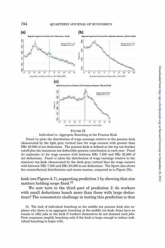
794 QUARTERLY JOURNAL OF ECONOMICS
FIGURE IXIndividual vs. Aggregate Bunching at the Pension Kink
Panel (a) plots the distribution of wage earnings relative to the pension kink(demarcated by the light gray vertical line) for wage earners with greater thanDKr 20,000 of net deductions. The pension kink is defined as the top tax bracketcutoff plus the maximum tax-deductible pension contribution in each year. Panel(b) replicates (a) for wage earners with between DKr 7,500 and DKr 25,000 ofnet deductions. Panel (c) plots the distribution of wage earnings relative to thestatutory top kink (demarcated by the dark gray vertical line) for wage earnerswith between DKr 7,500 and DKr 25,000 in net deductions. The figure alsoshowsthe counterfactual distributions and excess masses, computed as in Figure IIIa.
kink(seeFigureA.7), supportingprediction1 byshowingthat sizematters holding scope fixed.31
We now turn to the third part of prediction 2: do workerswith small deductions bunch more than those with large deduc-tions? The econometricchallenge in testing this prediction is that
31. The lack of individual bunching at the middle tax pension kink also ex-plains why there is no aggregate bunching at the middle tax kink: firms have noreason to offer jobs at the kink if workers themselves do not demand such jobs.Firm responses amplify bunching only if the kink is large enough to induce indi-vidual bunching to begin with.
at Harvard U
niversity on September 26, 2012
http://qje.oxfordjournals.org/D
ownloaded from

ADJUSTMENT COSTS AND LABOR SUPPLY ELASTICITIES 795
deductions themselves are endogenous. In particular, workerswith large deductions may have chosen their deductions in orderto reach the top tax kink. We address this endogeneity problemusing a grouping instrument. We compute the fraction of work-ers with deductions less than DKr 7,500 in magnitude for cells ofthepopulationdefinedbymarital status, gender, year, andage(indecades). We then divide workers intoten equal-width bins basedon the fraction of workers with small deductions in their groupand estimate the degree of bunching at the top kink (b) for work-ers in each of these ten bins.32 Figure X plots the estimated b vs.the fraction of workers with small deductions in the ten groups.The groups with small deductions exhibit much greater bunching:the slope of the fitted line in Figure X is statistically significantwith p < 0.01. This result confirms that tax incentives that af-fect a larger groupof workers generate large observedelasticities.Workers with small deductions can rely on aggregate bunching toreach the top kink, whereas workers with large deductions needto actively search for a less common job.
Furthersupportingtheimportanceofaggregatebunching, wefind that some of the heterogeneity in elasticities acrossdemographic groups (as in Figure IIIb) is driven by occupationalchoice. Forinstance, reweightingmen’s occupations tomatchthoseof women’s eliminates 50% of the gap in observed elasticities be-tween men and women (see Online Appendix Figure A.8).
Changes in the aggregate distribution of job offers alsoshapeearnings dynamics as the tax bracket changes. Tocharacterizede-fine an indicator for whether an individual’s change in wage earn-ings from year t to year t + 2 is within DKr 7500 (the width ofour bunching window) of the change in the top tax bracket cutofffrom year t to year t + 2. This indicator measures whether an in-dividual tracks the movement in the kink over time. Figure XIaplots the fraction of individuals who track the movement in thekink vs. the level of wage earnings in the base year relative tothestatutory kink. The propensity totrack the movement in the kinkis highest for individuals near the kink to begin with. Figure XIbreplicates Figure XIa forthepensionkink, focusingonindividualswith deductions greater than 20,000 in year t, as in Figure IXa.Individuals at the pension kink in year t do not have any excess
32. We exclude groups with a fraction of workers with small deductions in thebottomandtop5% of thedistribution, as therearetoofewobservations toestimateb in equal-width bins in the tails.
at Harvard U
niversity on September 26, 2012
http://qje.oxfordjournals.org/D
ownloaded from
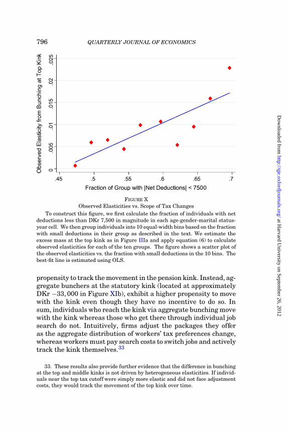
796 QUARTERLY JOURNAL OF ECONOMICS
FIGURE XObserved Elasticities vs. Scope of Tax Changes
To construct this figure, we first calculate the fraction of individuals with netdeductions less than DKr 7,500 in magnitude in each age-gender-marital status-yearcell. Wethengroupindividuals into10 equal-widthbins basedonthefractionwith small deductions in their group as described in the text. We estimate theexcess mass at the top kink as in Figure IIIa and apply equation (6) to calculateobserved elasticities for each of the ten groups. The figure shows a scatter plot ofthe observed elasticities vs. the fraction with small deductions in the 10 bins. Thebest-fit line is estimated using OLS.
propensitytotrackthemovement inthepensionkink. Instead, ag-gregate bunchers at the statutory kink (located at approximatelyDKr−33, 000 in Figure XIb), exhibit a higher propensity to movewith the kink even though they have no incentive to do so. Insum, individuals whoreachthekinkvia aggregatebunchingmovewith the kink whereas those whoget there through individual jobsearch do not. Intuitively, firms adjust the packages they offeras the aggregate distribution of workers’ tax preferences change,whereas workers must paysearchcosts toswitchjobs andactivelytrack the kink themselves.33
33. These results alsoprovide further evidence that the difference in bunchingat the top and middle kinks is not driven by heterogeneous elasticities. If individ-uals near the top tax cutoff were simply more elastic and did not face adjustmentcosts, they would track the movement of the top kink over time.
at Harvard U
niversity on September 26, 2012
http://qje.oxfordjournals.org/D
ownloaded from

ADJUSTMENT COSTS AND LABOR SUPPLY ELASTICITIES 797
FIGURE XIDynamics of Earnings Around the Top Tax Cutoff
These figures show how the propensity to track the movement in the top taxcutoffacross years varies across individuals. Toconstruct Panel (a), wefirst divideindividuals intobins of DKr 1000 in wage earnings in a given year t, and calculatethe fraction in each bin whose change in wage earnings from a year t to t + 2 fallswithin DKr 7,500 of the movement in the toptax bracket cutofffrom year t to t + 2.Panel (a) plots this fraction for wage earnings bins around the statutory top taxcutoff. Panel (b) replicates (a) for the pension kink, restricting the sample to wageearners with net deductions greater than DKr 20,000. It shows the fraction of in-dividuals whose change in wage earnings falls within DKr 7,500 of the movementin the pension kink for wage earnings bins around the pension kink.
at Harvard U
niversity on September 26, 2012
http://qje.oxfordjournals.org/D
ownloaded from
798 QUARTERLY JOURNAL OF ECONOMICS
We conclude that firm responses play a central role in shap-ing the effects of tax changes on equilibrium labor supply. Suchresponses may be particularly easy todetect in Denmark becausecollective bargaining facilitates the aggregation of workers’ taxpreferences. While collective bargaining is less common ineconomies suchas theU.S., technological constraints leadtohoursconstraints in all labor markets. The general lesson to be drawnfrom the evidence here is that these constraints are endogenousto the tax regime.
IV.C. Prediction 3: Correlation Between Individualand Aggregate Bunching
We test the third prediction of the model by examining thecorrelation between individual and aggregate bunching acrossoccupations. As above, wemeasureaggregatebunching bA
q inoccu-pation q by measuring the excess mass in the wage earnings dis-tribution at the statutory top tax cutoff for individuals who havemore than DKr 20,000 in deductions (and therefore have no in-centive to locate at the statutory kink). We measure individualbunching bI
q by the excess mass at the pension kink in the wageearnings distribution for individuals in occupation q with morethan DKr 20,000 in deductions, because this kink has near-zeroscope(ζ ' 0). Notethat bA
q andbIq areestimates of bunchingat two
different kinks for the same groupof individuals, andthus are notmechanically related.
Figure XII plots the estimates of bAq vs. estimates of bI
q acrossoccupations defined at the 2 digit ISCO level. The (unweighted)correlation between bA
q and bIq is 0.65 andis significantly different
from0 withp < 0.001. Inaregressionweightedbyoccupationsize,64% of the variation in bA
q is explainedby the variation in bIq. Note
that the few negative point estimates of bIq and bA
q are not signif-icantly different from zero. We cannot interpret the positive cor-relation in Figure XII as evidence that differences in individuals’preferences cause changes in the distribution of jobs offered asthey could also be driven by sorting of workers into occupationsthat suit theirtastes. Nevertheless, theevidenceis consistent withthe model’s prediction that firms (or unions) cater toworkers’ tax-distorted preferences in equilibrium.
IV.D. Self-Employed Individuals
Theself-employedareauseful comparisongroupbecausetheyfacemuchsmallerfrictions inadjustingtaxableincomethanwage
at Harvard U
niversity on September 26, 2012
http://qje.oxfordjournals.org/D
ownloaded from

ADJUSTMENT COSTS AND LABOR SUPPLY ELASTICITIES 799
FIGURE XIICorrelation Between Individual and Aggregate Bunching
This figure plots the amount of aggregate bunching (bAq ) vs. the amount of in-
dividual bunching (bIq) for all International Standard Classification of Occupation
codes at the twodigit level. Both aggregate andindividual bunching are estimatedon the subgroup of individuals with net deductions greater than DKr 20,000, as inFigure IXa. Individual bunching is the excess mass at the pension kink for thisgroup, while aggregate bunching is the excess mass at the statutory top tax cutofffor the same group. See Table A.1 for a list of the occupation codes.
earners. They are not subject tohours constraints anddonot needtosearchfora different jobtochangetheirearnings. Theycanalsoeasilychangereportedtaxableincomes, eitherbyshiftingrealizedincome across years or by under-reporting taxable incomes.34
Therefore, we expect that the model’s three predictions shouldnotapply to the self-employed.
Figure XIII replicates the key graphs shown above for theself-employed. Figure XIIIa shows that the self-employed exhibitextremely sharp bunching at the top kink, consistent with theirability to adjust their income more easily. The estimated excessmass is b = 18.4 at the top kink, dwarfing the excess mass
34. The Danish tax code allows the self-employed to shift some income acrossyears legally.
at Harvard U
niversity on September 26, 2012
http://qje.oxfordjournals.org/D
ownloaded from

800 QUARTERLY JOURNAL OF ECONOMICS
FIGURE XIIISelf-Employed Individuals
These figures include only individuals who report positive self-employmentincome. Panels (a) and (b) plot the taxable income distribution around the top andmiddle cutoffs from 1994–2001. Panel (c) plots the distribution of realized self-employment income around the statutory top tax cutoff for individuals with netdeductions greater than 20,000. Panel (d) replicates Figure X for individuals withpositive self-employment income, with the y axis scaled to have the same rangerelative to the mean observed elasticity as in Figure X.
for wage earners and implying an observed elasticity of 0.24.Figure XIIIb shows that unlike wage earners, the self-employedalsobunch sharply at the middle tax kink. The observedelasticityat the middle kink is 0.10. We believe that the observed elasticityat the middle kink is smaller than that at the top kink becausecapital income is subject to the middle tax but not the top tax.Self-employed individuals are allowed to reclassify some of theirprofits as capital income, creating an added margin of response atthe toptax cutoff. Consistent with this explanation, self-employedindividuals with capital income less than DKr 1,000 in magnitudehave an observed elasticity of 0.16 at the middle kink vs. 0.20 atthe top kink.
at Harvard U
niversity on September 26, 2012
http://qje.oxfordjournals.org/D
ownloaded from
ADJUSTMENT COSTS AND LABOR SUPPLY ELASTICITIES 801
Figure XIIIc tests for aggregate bunching by plotting the in-come distribution around the statutory kink for self-employed in-dividuals with deductions larger than DKr 20,000. Unlike wageearners, self employed individuals with large deductions exhibitno excess mass around the statutory kink. As a result, selfemployed individuals with common tax preferences (small deduc-tions) bunch just as much as those with uncommon tax prefer-ences (large deductions). This is shown in Figure XIIId, whichis constructed using mean group deductions in the same way asFigure X.
These “placebo tests” confirm that our three predictions donot apply to the self-employed.35 Some of the bunching amongthe self-employedis driven by intertemporal shifting andevasion.LeMaire and Schjerning (2007) demonstrate using the same Dan-ishdata that theself-employedadjust theirretainedearnings andprofit distributions over time to remain below the top tax thresh-old in each year. Kleven et al. (2010) uncover substantial taxevasion among the self-employed and estimate that 40% of thebunchingat thetopkinkis drivenbytaxevasion. Eliminatingthisevasion component of bunching at the top kink implies ataxable income elasticity for the self employed of 0.14. Regard-less of which margin the self employed use, we can conclude thatfrictions significantly attenuate observed elasticities: the size andscope of tax changes matters less for margins of behavior with lowfrictions (changing reported taxable income or self-employmentearnings) than for margins with higher frictions (changing wageearnings).
V. CONCLUSION
This paper has shown that the effects of tax policies on laborsupply are shaped by adjustment costs and hours constraintsendogenously chosen by firms. Because of these forces, modernmicroeconometric methods of estimating elasticities – focusingon policy changes that affect a subgroup of workers – may under-estimate the “structural” elasticities that control steady-state responses.
35. Furthermore, we find that individuals who switch between self-employment and wage earning have a much greater propensity to bunch at kinksin the years when they are self employed.
at Harvard U
niversity on September 26, 2012
http://qje.oxfordjournals.org/D
ownloaded from

802 QUARTERLY JOURNAL OF ECONOMICS
Ourempirical analysis does not yieldanestimateof thestruc-tural (macro) elasticity. In Chetty et al. (2009), we calibrate amoregeneral versionofthemodel presentedhere. Wefindthat thestructural elasticity that matches the evidence is an order of mag-nitude larger than the observed elasticity at the top kink. Intu-itively, a small ε cannot produce substantial variation in observedelasticities across tax changes of different size and scope becausethe costs of deviating from optimal hours are very large when ε issmall. In future work, it would be useful to identify ε more pre-cisely by structurally estimating a more realistic dynamic modelof labor supply with frictions.
It would also be interesting to explore the normative impli-cations of adjustment costs and firm responses. For example, theefficiency cost of a tax levied on one group of workers may dependnot just upon their elasticities but also upon those of theirco-workers if firms are constrained to offer similar packages todifferent workers. Another example concerns the prediction thatit is optimal to levy higher tax rates on men than women becausethey are less elastic (Boskin and Sheshinski 1983; Alesina, Ichinoand Karabarbounis 2007; Kleven, Kreiner, and Saez 2009). If thedifference in observedelasticities across genders is causedby het-erogeneity in occupational frictions rather than tastes, there maybe less justification for higher taxes on secondary earners insteady state.
Finally, the results here call for caution in using quasi-experiments that apply to small subgroups to learn about theeffects of economic policies on behavior. In settings with rigid in-stitutional structures and frictions in adjustment, the steady-state effects of policies implemented at an economy-widelevel could differ substantially from the effects of suchexperiments.
HARVARD UNIVERSITY AND NBERHARVARD UNIVERSITY AND NBERHARVARD UNIVERSITY AND CAMSTANFORD UNIVERSITY AND NBER
REFERENCES
Altonji, Joseph G., and Christina H. Paxson, “Labor Supply Preferences, HoursConstraints, and Hours-Wage Trade-Offs,” Journal of Labor Economics, 6(1988), 254–276.
at Harvard U
niversity on September 26, 2012
http://qje.oxfordjournals.org/D
ownloaded from
ADJUSTMENT COSTS AND LABOR SUPPLY ELASTICITIES 803
Alesina, Alberto F., Edward L. Glaeser, and Bruce Sacerdote, “Work and LeisureintheU.S. andEurope: WhySoDifferent?”in NBER Macroeconomics Annual,eds. M. Gertler and K. Rogoff, 20 (2005), 1–64.
Alesina, Alberto F., Andrea Ichino, and Loukas Karabarbounis, “Gender-BasedTaxation and the Division of Family Chores,” NBER Working Paper 13638(2007).
Andersen, Torben M., and Michael Svarer, “Flexicurity: Labour Market Perfor-mance in Denmark,” CESifo Economic Studies, 53 (2007), 389–429.
Blundell, Richard, and Thomas MaCurdy, “Labor Supply: A Reviewof AlternativeApproaches,” in Handbook of Labor Economics, Orley Ashenfelter and DavidCard eds., (1999).
Boskin, Michael J., andEytan Sheshinski, “Optimal Tax Treatment of the Family:Married Couples,” Journal of Public Economics, 20 (1983), 281–297.
Chetty, Raj, “Bounds on Elasticities with Optimization Frictions: A Synthesis ofMicroandMacroEvidenceonLaborSupply,”NBERWorkingPaperNo. 15616(2011).
Chetty, Raj, “Is the Taxable Income Elasticity Sufficient to Calculate DeadweightLoss? The Implications of Evasion and Avoidance,” American Economic Jour-nal: Economic Policy, 1 (2009), 31–52.
Chetty, Raj, John N. Friedman, Tore Olsen, and Luigi Pistaferri, “AdjustmentCosts, Firm Responses, and Micro vs. Macro Labor Supply Elasticities: Ev-idence from Danish Tax Records,” NBER Working Paper No. 15617, 2009.
Chetty, Raj, Adam Guren, Day Manoli, and Andrea Weber, “Are Micro and MacroLabor Supply Elasticities Consistent? A Review of Evidence on the Intensiveand Extensive Margins.” American Economic Review, forthcoming, May 2011.
Chetty, Raj, and Emmanuel Saez, “Teaching the Tax Code: Earnings Responsesto an Experiment with EITC Recipients,” NBER Working Paper No. 14836,2009.
Cogan, John, “Fixed Costs and Labor Supply,” Econometrica, 49 (1981), 945–963.Davis, Steven, and Magnus Henrekson, “Tax Effects on Work Activity, Industry
Mix and Shadow Economy Size: Evidence from Rich-Country Comparisons,”in Labour Supply and Incentives to Work in Europe, Ramon Gomez Salvador,Ana Lamo, Barbara Petrongolo, Melanie Ward, and Etienne Wasmer eds.(Northamption, MA: Edward Elgar Publishing, 2005).
Dickens, William T., and Shelly J. Lundberg, “Hours Restrictions and LaborSupply,” International Economic Review, 34 (1993), 169–192.
Earle, John S. and John Pencavel, “Hours of Work and Trade Unionism,” Journalof Labor Economics 8 (1990), S150–74.
Farber, Henry S., “Is TomorrowAnother Day? The Labor Supply of NewYork CityCabdrivers,” Journal of Political Economy, 113 (2005), 46–82.
Fehr, Ernst, and Lorenz Goette, “Do Workers Work More if Wages Are High? Evi-dence from a Randomized Field Experiment,” American Economic Review, 97(2007), 298–317.
Feldstein, Martin, “Tax Avoidance and the Deadweight Loss of the Income Tax.”Review of Economics and Statistics, 81 (1999), 674–680.
Goolsbee, Austin, “What Happens When You Tax the Rich? Evidence from Execu-tive Compensation,” Journal of Political Economy, 108 (2000), 352–378.
Gruber, Jonathan, and Emmanuel Saez, “The Elasticity of Taxable Income: Evi-dence and Implications,” Journal of Public Economics, 84 (2002), 1–32.
Ham, John C., “Estimation of a Labour Supply Model with Censoring Due toUnemployment and Underemployment,” Review of Economic Studies, 49(1982), 335–354.
Hansen, Claus Thustrup. “Lower Tax Progression, Longer Hours and HigherWages.” Scandinavian Journal of Economics, 101 (1999), 49–65.
Hausman, JerryA., “LaborSupply,”inHow Taxes Affect Economic Behavior, HenryAaron and Joseph Pechman eds. (Washington D.C.: The Brookings Institu-tion, 1981).
Holmlund, Bertil, andMartinSoderstrom, “EstimatingDynamicIncomeResponsesto Tax Reforms: Swedish Evidence,” mimeo, Uppsala University, 2008.
Kleven, Henrik, and Claus Kreiner, “Welfare and Taxation” in Tax, Work, andEquality: An Investigation of the Danish Tax and Welfare System, TorbenTranaes ed. (Copenhagen: Gyldendal, 2006)
at Harvard U
niversity on September 26, 2012
http://qje.oxfordjournals.org/D
ownloaded from

804 QUARTERLY JOURNAL OF ECONOMICS
Kleven, Henrik, Martin Knudsen, Claus T. Kreiner, Søren Pedersen, and Em-manuel Saez, “Unwilling or Unable to Cheat? Evidence from a RandomizedTax Audit Experiment in Denmark,” NBER Working Paper 15769, 2010.
Kleven, Henrik, Claus Kreiner, and Emmanuel Saez, “The Optimal Income Taxa-tion of Couples,” Econometrica, 77 (2009), 537–560.
Kleven, Henrik and Esben A. Schultz, “Estimating Taxable Income Responses Us-ing Danish Tax Reforms,” mimeo, London School of Economics, 2010.
LeMaire, Daniel, and Bertel Schjerning, “Earnings, Uncertainty, and the Self-Employment Choice,” CBER Discussion Paper DP 2007–04, 2007.
Lindbeck, Assar, “Welfare State Disincentives with Endogenous Habits andNorms,” The Scandinavian Journal of Economics, 97 (1995), 477–494.
MaCurdy, Thomas, David Green, and Harry Paarsch, “Assessing EmpiricalApproaches for Analyzing Taxes and Labor Supply,” The Journal of HumanResources, 25 (1990), 415–490.
Ministry of Taxation, Skatteberegningsreglerne, før og nu, http://www.skm.dk/public/dokumenter/Tal45/Skatteberegning90/Skatteberegningsreglerne 2.pdf, 2002.
Moffitt, Robert A., “The Econometrics of Kinked Budget Constraints,” Journal ofEconomic Perspectives, 4 (1990), 119–139.
Oettinger, GeraldS., “AnEmpirical Analysis of theDailyLaborSupplyof StadiumVendors,” Journal of Political Economy, 107 (1999), 360–392.
Rogerson, Richard. “Comment onWorkandLeisureintheU.S. andEurope: Whysodifferent?”, in NBER Macroeconomics Annual, eds. M. Gertler and K. Rogoff,20 (2005), 79–95.
Rogerson, Richard, andJohanna Wallenius, “MicroandMacroElasticities ina LifeCycle Model with Taxes,” Journal of Economic Theory, 144 (2009),2277–2292.
Rosen, Harvey S., “Taxes in a Labor Supply Model with Joint Wage-Hours Deter-mination,” Econometrica , 44 (1976), 485–507.
Saez, Emmanuel, “DoTaxpayers Bunchat KinkPoints?”American Economic Jour-nal: Economic Policy, 2 (2010), 180–212.
Saez, Emmanuel, Joel B. Slemrod, and Seth H. Giertz, “The Elasticity of TaxableIncome with Respect to Marginal Tax Rates: A Critical Review,” Journal ofEconomic Literature, forthcoming, 2010.
Slemrod, Joel B., “Income Creation or Income Shifting? Behavioral Responses tothe Tax Reform Act of 1986,” American Economic Review, 85 (1995), 175–180
Slemrod, Joel B., and Shlomo Yitzhaki, “Tax avoidance, evasion, and administra-tion,” in Handbook of Public Economics, Alan Auerbach and Martin Feldsteineds. (Amsterdam: North-Holland, 2002).
at Harvard U
niversity on September 26, 2012
http://qje.oxfordjournals.org/D
ownloaded from