admission control for independently-authored realtime
TRANSCRIPT
Admission Control for Independently-authored Realtime
Applications
by
Robert Kroeger
A thesispresented to the University of Waterloo
in fulfilment of thethesis requirement for the degree of
Doctor of Philosophyin
Computer Science
Waterloo, Ontario, Canada, 2004
c©Robert Kroeger 2004

AUTHOR’S DECLARATION FOR ELECTRONIC SUBMISSION OF A THESIS
I hereby declare that I am the sole author of this thesis. This is a true copy of the thesis,including any required final revisions, as accepted by my examiners.
I understand that my thesis may be made electronically available to the public.
ii
Abstract
This thesis presents the LiquiMedia operating system architecture. LiquiMedia is specializedto schedule multimedia applications. Because they generate output for a human observer,multimedia applications such as video games, video conferencing and video players have bothunique scheduling requirements and unique allowances: a multimedia stream must synchro-nize sub-streams generated for different sensory modalities within 20 milliseconds, it is notsuccessfully segregated until it has existed for over 200 milliseconds and tolerates occasionalscheduling failures.
LiquiMedia is specialized around these requirements and allowances. First, LiquiMediasynchronizes multimedia tasks by invoking them from a shared realtime timer interrupt. Sec-ond, owing to multimedia’s tolerance of scheduling failures, LiquiMedia schedules tasks basedon a probabilistic model of their running times. Third, LiquiMedia can infer per-task modelswhile a user is segregating the streams that the tasks generate.
These specializations provide novel capabilities: up to 2.5 times higher utilization than RMSscheduling, use of an atomic task primitive 9.5 times more efficient than preemptive threading,and most importantly, the ability to schedule arbitrary tasks to a known probability of realtimeexecution without a priori knowledge of their running times.
iii

Acknowledgements
Friends, money and academic advice got me through this thesis. Slowly. All deserve mythanks.
First, on the subject of academic advice, I thank my supervisor, Bill Cowan for his guidance,insight and particularly his patience. Also, I thank my committee for their prompt and valuablefeedback.
As for money, many organizations have supported this research — I am grateful for thesupport of NSERC, IBM, ITRC and LiquiMedia Inc. Ironically, I am also grateful for the lackof money: the stock crash of 2001 bankrupted my salaried thesis avoidance opportunity.
I would have given up long ago without the encouragement of family and friends: manyCGL members over the years, Tresidder alumni and the yawners. Of these, special thanksmust go out to Ian Bell, Igor Benko, Celine Latulipe, Peter Mayo, Alex Nicolaou and ShinjiSato for (sometimes inadvertently) convincing me to continue.
Lastly, thanks to Peter Kokkovas for the totally cool name.
iv

Trademarks
HRV, Java, JMF, JavaBeans, NeWS, VIS, TAAC-1, Solaris and SPARC are trademarks ofSun Microsystems Inc.
DirectX, DirectShow, COM, Windows NT, Windows 2000 and Vizact are trademarks ofMicrosoft Inc.
QuickTime, Core Image, Aqua and MacOS X are trademarks of Apple Computer Inc.
LiquiMedia, LiquiOS and MVM were trademarks of LiquiMedia Inc.
Pentium, SSE and MMX are trademarks of Intel Inc.
POSIX and UNIX are trademarks of the X/Open group.
WindRiver and VxWorks are trademarks of WindRiver Inc.
Virtuoso and Eonic are trademarks of Eonic Systems Inc.
Precise is a trademark of Precise Software Technologies.
SPARK is a trademark of Realtime Microsystems Inc..
HP, DEC, VMS and Alpha are trademarks of HP Inc.
Qualcomm and BREW are trademarks of Qualcomm Inc.
Streammaster and Motorola are trademarks of Motorola Inc.
TeraLogic is a trademark of TeraLogic Inc.
Mwave is a trademark of Texas Instruments Inc.
Chromatic is possibly a trademark of ATI Inc.
Trimedia is a trademark of Philips Inc.
SGI, REACT and IRIX are trademarks or SGI Inc.
Harmony is a trademark reserved for the Crown.
v

Contents
1 Introduction 1
1.1 Information Streams . . . . . . . . . . . . . . . . . . . . . . . . . . . . . . . . . 1
1.2 Specialized Design . . . . . . . . . . . . . . . . . . . . . . . . . . . . . . . . . . 3
1.2.1 The Recital Model . . . . . . . . . . . . . . . . . . . . . . . . . . . . . . 4
1.2.2 Design Principles . . . . . . . . . . . . . . . . . . . . . . . . . . . . . . . 4
1.3 Applications . . . . . . . . . . . . . . . . . . . . . . . . . . . . . . . . . . . . . . 8
1.3.1 On the Desktop . . . . . . . . . . . . . . . . . . . . . . . . . . . . . . . . 8
1.3.2 The Embedded Space . . . . . . . . . . . . . . . . . . . . . . . . . . . . 11
1.4 LiquiMedia Overview . . . . . . . . . . . . . . . . . . . . . . . . . . . . . . . . . 13
1.5 Organization . . . . . . . . . . . . . . . . . . . . . . . . . . . . . . . . . . . . . 15
2 The RTOS Design Space 17
2.1 Taxonomy Overview . . . . . . . . . . . . . . . . . . . . . . . . . . . . . . . . . 18
2.2 Task Abstraction . . . . . . . . . . . . . . . . . . . . . . . . . . . . . . . . . . . 21
2.2.1 Performers . . . . . . . . . . . . . . . . . . . . . . . . . . . . . . . . . . 22
2.2.2 Preemptive Threads . . . . . . . . . . . . . . . . . . . . . . . . . . . . . 23
2.2.3 Non-preemptive Threads . . . . . . . . . . . . . . . . . . . . . . . . . . . 23
2.3 Deadline Sensitivity . . . . . . . . . . . . . . . . . . . . . . . . . . . . . . . . . 24
2.4 Externalization . . . . . . . . . . . . . . . . . . . . . . . . . . . . . . . . . . . . 25
2.4.1 Time-Triggered . . . . . . . . . . . . . . . . . . . . . . . . . . . . . . . . 26
2.4.2 Event-Triggered . . . . . . . . . . . . . . . . . . . . . . . . . . . . . . . 26
vi
2.5 Scheduling . . . . . . . . . . . . . . . . . . . . . . . . . . . . . . . . . . . . . . . 27
2.5.1 Distributed Scheduling . . . . . . . . . . . . . . . . . . . . . . . . . . . . 28
2.5.2 Static Priority Scheduling . . . . . . . . . . . . . . . . . . . . . . . . . . 28
2.5.3 EDF Scheduling . . . . . . . . . . . . . . . . . . . . . . . . . . . . . . . 29
2.5.4 Rate-Based Scheduling . . . . . . . . . . . . . . . . . . . . . . . . . . . . 30
2.6 Admission Control . . . . . . . . . . . . . . . . . . . . . . . . . . . . . . . . . . 33
2.6.1 Admission Control Opportunities . . . . . . . . . . . . . . . . . . . . . . 33
2.6.2 Absent Admission Control . . . . . . . . . . . . . . . . . . . . . . . . . . 34
2.6.3 Declarative Admission Control . . . . . . . . . . . . . . . . . . . . . . . 34
2.6.4 Statistical Admission Control . . . . . . . . . . . . . . . . . . . . . . . . 34
2.6.5 Mechanical Admission Control . . . . . . . . . . . . . . . . . . . . . . . 35
2.7 Processor Partitioning . . . . . . . . . . . . . . . . . . . . . . . . . . . . . . . . 35
2.7.1 Hardware Partitioning . . . . . . . . . . . . . . . . . . . . . . . . . . . . 35
2.7.2 Hierarchical Partitioning . . . . . . . . . . . . . . . . . . . . . . . . . . . 36
2.7.3 Task Partitioning . . . . . . . . . . . . . . . . . . . . . . . . . . . . . . . 36
2.8 Inter-process Communication . . . . . . . . . . . . . . . . . . . . . . . . . . . . 36
2.8.1 Divisible Task IPC . . . . . . . . . . . . . . . . . . . . . . . . . . . . . . 37
2.8.2 Atomic Task IPC . . . . . . . . . . . . . . . . . . . . . . . . . . . . . . . 37
2.9 Summary . . . . . . . . . . . . . . . . . . . . . . . . . . . . . . . . . . . . . . . 38
3 Previous Work 39
3.1 Embedded Operating Systems . . . . . . . . . . . . . . . . . . . . . . . . . . . . 39
3.1.1 Cyclic Executives . . . . . . . . . . . . . . . . . . . . . . . . . . . . . . . 40
3.1.2 RMS Operating Systems . . . . . . . . . . . . . . . . . . . . . . . . . . . 42
3.2 Hardware Partitioning Operating Systems . . . . . . . . . . . . . . . . . . . . . 43
3.3 Media Generation Frameworks . . . . . . . . . . . . . . . . . . . . . . . . . . . 46
3.4 Distributed Scheduling Operating Systems . . . . . . . . . . . . . . . . . . . . . 50
3.5 Hierarchical Partitioning Operating Systems . . . . . . . . . . . . . . . . . . . . 52
3.6 Task Partitioning Operating Systems . . . . . . . . . . . . . . . . . . . . . . . . 53
vii
3.6.1 Realtime Mach and Descendants . . . . . . . . . . . . . . . . . . . . . . 53
3.6.2 Rialto . . . . . . . . . . . . . . . . . . . . . . . . . . . . . . . . . . . . . 55
3.6.3 YARTOS and DiRT . . . . . . . . . . . . . . . . . . . . . . . . . . . . . 57
3.6.4 SMART . . . . . . . . . . . . . . . . . . . . . . . . . . . . . . . . . . . . 58
3.6.5 BERT . . . . . . . . . . . . . . . . . . . . . . . . . . . . . . . . . . . . . 58
3.6.6 Summary . . . . . . . . . . . . . . . . . . . . . . . . . . . . . . . . . . . 58
3.7 Statistical Admission Control . . . . . . . . . . . . . . . . . . . . . . . . . . . . 59
3.7.1 DSAC OSs . . . . . . . . . . . . . . . . . . . . . . . . . . . . . . . . . . 59
3.7.2 ESAC OSs . . . . . . . . . . . . . . . . . . . . . . . . . . . . . . . . . . 61
3.8 Summary . . . . . . . . . . . . . . . . . . . . . . . . . . . . . . . . . . . . . . . 62
4 Architecture Overview 65
4.1 Taxonomic Position . . . . . . . . . . . . . . . . . . . . . . . . . . . . . . . . . 66
4.2 Soft Realtime . . . . . . . . . . . . . . . . . . . . . . . . . . . . . . . . . . . . . 69
4.3 Hierarchical Partitioning . . . . . . . . . . . . . . . . . . . . . . . . . . . . . . . 70
4.4 Realtime Performers . . . . . . . . . . . . . . . . . . . . . . . . . . . . . . . . . 72
4.4.1 Practical and Natural . . . . . . . . . . . . . . . . . . . . . . . . . . . . 72
4.4.2 Efficient . . . . . . . . . . . . . . . . . . . . . . . . . . . . . . . . . . . . 72
4.5 Non-realtime Threads . . . . . . . . . . . . . . . . . . . . . . . . . . . . . . . . 73
4.6 Conduit IPC . . . . . . . . . . . . . . . . . . . . . . . . . . . . . . . . . . . . . 73
4.7 Task-partitioned Performers . . . . . . . . . . . . . . . . . . . . . . . . . . . . . 75
4.8 Schedule Graph . . . . . . . . . . . . . . . . . . . . . . . . . . . . . . . . . . . . 75
4.9 Statistical Admission Control . . . . . . . . . . . . . . . . . . . . . . . . . . . . 78
4.9.1 Lifetime Admission Control . . . . . . . . . . . . . . . . . . . . . . . . . 79
4.10 Instantaneous Admission Control . . . . . . . . . . . . . . . . . . . . . . . . . . 81
4.11 Satisfies Fundamental Principles . . . . . . . . . . . . . . . . . . . . . . . . . . 83
4.12 Summary . . . . . . . . . . . . . . . . . . . . . . . . . . . . . . . . . . . . . . . 84
viii
5 Implementation 85
5.1 Extending Solaris . . . . . . . . . . . . . . . . . . . . . . . . . . . . . . . . . . . 85
5.2 Implementation Structures . . . . . . . . . . . . . . . . . . . . . . . . . . . . . . 88
5.2.1 Conduits . . . . . . . . . . . . . . . . . . . . . . . . . . . . . . . . . . . 88
5.2.2 Exception Handlers . . . . . . . . . . . . . . . . . . . . . . . . . . . . . 88
5.2.3 Applications . . . . . . . . . . . . . . . . . . . . . . . . . . . . . . . . . 89
5.2.4 Memory Management . . . . . . . . . . . . . . . . . . . . . . . . . . . . 89
5.2.5 Timing and Measurement . . . . . . . . . . . . . . . . . . . . . . . . . . 90
5.3 Implementation Strategy . . . . . . . . . . . . . . . . . . . . . . . . . . . . . . . 91
5.4 The Scheduler Simulator . . . . . . . . . . . . . . . . . . . . . . . . . . . . . . . 91
5.5 Summary . . . . . . . . . . . . . . . . . . . . . . . . . . . . . . . . . . . . . . . 92
6 Performance Measurements 93
6.1 Apparatus and Methodology . . . . . . . . . . . . . . . . . . . . . . . . . . . . 93
6.1.1 Metrics . . . . . . . . . . . . . . . . . . . . . . . . . . . . . . . . . . . . 93
6.1.2 Overview of Tests . . . . . . . . . . . . . . . . . . . . . . . . . . . . . . 95
6.1.3 Test Performers . . . . . . . . . . . . . . . . . . . . . . . . . . . . . . . . 95
6.1.4 Realtime Test Details . . . . . . . . . . . . . . . . . . . . . . . . . . . . 101
6.1.5 Summary . . . . . . . . . . . . . . . . . . . . . . . . . . . . . . . . . . . 104
6.2 Partitioning . . . . . . . . . . . . . . . . . . . . . . . . . . . . . . . . . . . . . . 104
6.3 Synchronous Realtime . . . . . . . . . . . . . . . . . . . . . . . . . . . . . . . . 105
6.4 Ultra-Fine Granularity Performers . . . . . . . . . . . . . . . . . . . . . . . . . 111
6.4.1 Conductor and Performer Overhead . . . . . . . . . . . . . . . . . . . . 113
6.4.2 Comparison . . . . . . . . . . . . . . . . . . . . . . . . . . . . . . . . . . 113
6.5 Modularity . . . . . . . . . . . . . . . . . . . . . . . . . . . . . . . . . . . . . . 115
6.5.1 Convergence . . . . . . . . . . . . . . . . . . . . . . . . . . . . . . . . . 116
6.5.2 Instantaneous Admission Control . . . . . . . . . . . . . . . . . . . . . . 123
6.5.3 Lifetime Admission Control . . . . . . . . . . . . . . . . . . . . . . . . . 123
6.5.4 Feedback and Schedule Convergence . . . . . . . . . . . . . . . . . . . . 126
6.6 Summary . . . . . . . . . . . . . . . . . . . . . . . . . . . . . . . . . . . . . . . 128
ix
7 Future Work 129
7.1 Experimentation and Analysis . . . . . . . . . . . . . . . . . . . . . . . . . . . . 129
7.1.1 Scheduler Operation . . . . . . . . . . . . . . . . . . . . . . . . . . . . . 129
7.1.2 Feedback Tests . . . . . . . . . . . . . . . . . . . . . . . . . . . . . . . . 130
7.1.3 Varied Loadings . . . . . . . . . . . . . . . . . . . . . . . . . . . . . . . 131
7.1.4 Expanding the Envelope . . . . . . . . . . . . . . . . . . . . . . . . . . . 131
7.1.5 Comparisons . . . . . . . . . . . . . . . . . . . . . . . . . . . . . . . . . 132
7.1.6 Time Series Analysis . . . . . . . . . . . . . . . . . . . . . . . . . . . . . 132
7.2 Prototype Enhancements . . . . . . . . . . . . . . . . . . . . . . . . . . . . . . 132
7.2.1 Reducing Overhead . . . . . . . . . . . . . . . . . . . . . . . . . . . . . 132
7.2.2 Timing . . . . . . . . . . . . . . . . . . . . . . . . . . . . . . . . . . . . 133
7.2.3 Enhanced Conduits . . . . . . . . . . . . . . . . . . . . . . . . . . . . . 133
7.2.4 Per-Performer Firmness . . . . . . . . . . . . . . . . . . . . . . . . . . . 134
7.2.5 Instrumentation . . . . . . . . . . . . . . . . . . . . . . . . . . . . . . . 134
7.2.6 Processor Redistribution . . . . . . . . . . . . . . . . . . . . . . . . . . . 134
7.3 Multiprocessor Support . . . . . . . . . . . . . . . . . . . . . . . . . . . . . . . 135
7.3.1 Multiple Conductors . . . . . . . . . . . . . . . . . . . . . . . . . . . . . 135
7.3.2 NUMA . . . . . . . . . . . . . . . . . . . . . . . . . . . . . . . . . . . . 137
7.4 DAG Scheduling . . . . . . . . . . . . . . . . . . . . . . . . . . . . . . . . . . . 137
7.5 Bandwidth Allocation . . . . . . . . . . . . . . . . . . . . . . . . . . . . . . . . 137
7.6 Native Implementation . . . . . . . . . . . . . . . . . . . . . . . . . . . . . . . . 138
7.7 Realtime Java VM . . . . . . . . . . . . . . . . . . . . . . . . . . . . . . . . . . 139
7.7.1 Garbage Collection . . . . . . . . . . . . . . . . . . . . . . . . . . . . . . 139
7.7.2 Tear-Down . . . . . . . . . . . . . . . . . . . . . . . . . . . . . . . . . . 139
7.7.3 I/O . . . . . . . . . . . . . . . . . . . . . . . . . . . . . . . . . . . . . . 140
7.8 Generative Operating Systems . . . . . . . . . . . . . . . . . . . . . . . . . . . 140
7.9 Summary . . . . . . . . . . . . . . . . . . . . . . . . . . . . . . . . . . . . . . . 141
x

8 Conclusions 143
8.1 Design Principles . . . . . . . . . . . . . . . . . . . . . . . . . . . . . . . . . . . 144
8.2 Design Aspects . . . . . . . . . . . . . . . . . . . . . . . . . . . . . . . . . . . . 144
8.3 Summary . . . . . . . . . . . . . . . . . . . . . . . . . . . . . . . . . . . . . . . 147
Bibliography 149
A Standard Nomenclature 163
B Architecture Details 169
B.1 Performers . . . . . . . . . . . . . . . . . . . . . . . . . . . . . . . . . . . . . . . 169
B.2 Statistical Inference . . . . . . . . . . . . . . . . . . . . . . . . . . . . . . . . . 170
B.2.1 Chebyshev’s Inequality . . . . . . . . . . . . . . . . . . . . . . . . . . . . 171
B.2.2 Sample Statistics Corrections . . . . . . . . . . . . . . . . . . . . . . . . 172
B.3 The Conductor . . . . . . . . . . . . . . . . . . . . . . . . . . . . . . . . . . . . 174
B.3.1 Interfaces . . . . . . . . . . . . . . . . . . . . . . . . . . . . . . . . . . . 174
B.3.2 Conductor Operation Overview . . . . . . . . . . . . . . . . . . . . . . . 177
B.3.3 Schedule Graphs . . . . . . . . . . . . . . . . . . . . . . . . . . . . . . . 177
B.3.4 Scheduling Function . . . . . . . . . . . . . . . . . . . . . . . . . . . . . 180
B.3.5 Instantaneous Admission Control . . . . . . . . . . . . . . . . . . . . . . 181
B.3.6 Statistical Profile Data . . . . . . . . . . . . . . . . . . . . . . . . . . . . 182
B.3.7 Reentrant Operation . . . . . . . . . . . . . . . . . . . . . . . . . . . . . 184
B.4 Scheduler . . . . . . . . . . . . . . . . . . . . . . . . . . . . . . . . . . . . . . . 188
B.4.1 Schedule Data Structures . . . . . . . . . . . . . . . . . . . . . . . . . . 188
B.4.2 Graph Construction . . . . . . . . . . . . . . . . . . . . . . . . . . . . . 190
B.4.3 Schedule Assembly . . . . . . . . . . . . . . . . . . . . . . . . . . . . . . 191
B.4.4 Restructuring . . . . . . . . . . . . . . . . . . . . . . . . . . . . . . . . . 193
B.4.5 Lifetime Admission Control . . . . . . . . . . . . . . . . . . . . . . . . . 197
B.4.6 Life Cycle and Feedback . . . . . . . . . . . . . . . . . . . . . . . . . . . 198
xi
C Windows NT Scheduling Failures 201
C.1 Apparatus . . . . . . . . . . . . . . . . . . . . . . . . . . . . . . . . . . . . . . . 201
C.2 Procedure . . . . . . . . . . . . . . . . . . . . . . . . . . . . . . . . . . . . . . . 201
C.3 Results . . . . . . . . . . . . . . . . . . . . . . . . . . . . . . . . . . . . . . . . . 202
D LiquiMedia Inc. 203
D.1 The Company . . . . . . . . . . . . . . . . . . . . . . . . . . . . . . . . . . . . . 203
D.2 Research . . . . . . . . . . . . . . . . . . . . . . . . . . . . . . . . . . . . . . . . 204
D.3 Developments . . . . . . . . . . . . . . . . . . . . . . . . . . . . . . . . . . . . . 204
D.3.1 Audioplayer Lessons . . . . . . . . . . . . . . . . . . . . . . . . . . . . . 206
D.4 Summary . . . . . . . . . . . . . . . . . . . . . . . . . . . . . . . . . . . . . . . 206
E PDF Statistical Scheduling 209
E.1 PDF-style Estimation . . . . . . . . . . . . . . . . . . . . . . . . . . . . . . . . 209
E.2 Normal Distribution . . . . . . . . . . . . . . . . . . . . . . . . . . . . . . . . . 210
F Testing Summary 213
F.1 Introduction . . . . . . . . . . . . . . . . . . . . . . . . . . . . . . . . . . . . . . 213
F.1.1 Test Performers . . . . . . . . . . . . . . . . . . . . . . . . . . . . . . . . 213
F.2 Unit Testing . . . . . . . . . . . . . . . . . . . . . . . . . . . . . . . . . . . . . . 213
F.3 Integration Testing . . . . . . . . . . . . . . . . . . . . . . . . . . . . . . . . . . 214
G Approximating wcet(p) 219
xii
List of Tables
1.1 Expectation delay of common consumer media devices. . . . . . . . . . . . . . . 2
2.1 Relationships between design aspects. . . . . . . . . . . . . . . . . . . . . . . . 20
6.1 Utilization of standard test performers . . . . . . . . . . . . . . . . . . . . . . . 107
6.2 Utilizations of WCET and Chebyshev estimators. . . . . . . . . . . . . . . . . . 109
6.3 Audio performer utilization levels. . . . . . . . . . . . . . . . . . . . . . . . . . 111
6.4 Comparison of performer and thread overhead. . . . . . . . . . . . . . . . . . . 115
6.5 Composition of randomly-generated schedules. . . . . . . . . . . . . . . . . . . 120
B.1 Overflow-free Integer Sizes . . . . . . . . . . . . . . . . . . . . . . . . . . . . . . 183
E.1 Normal Score Correlations . . . . . . . . . . . . . . . . . . . . . . . . . . . . . . 211
xiii
List of Figures
1.1 Expectation and segregation delays in context. . . . . . . . . . . . . . . . . . . 3
1.2 Recital Model . . . . . . . . . . . . . . . . . . . . . . . . . . . . . . . . . . . . . 4
1.3 Hardware partitioning vs. software partitioning . . . . . . . . . . . . . . . . . . 12
2.1 The three basic DS-Tree diagrammatic conventions. . . . . . . . . . . . . . . . 18
2.2 Complete RTOS design space. . . . . . . . . . . . . . . . . . . . . . . . . . . . . 19
2.3 Threads permit multiple slices. . . . . . . . . . . . . . . . . . . . . . . . . . . . 21
2.4 Threaded multi-tasking. . . . . . . . . . . . . . . . . . . . . . . . . . . . . . . . 22
2.5 Coupling and divisibility in task abstractions. . . . . . . . . . . . . . . . . . . . 24
2.6 Incomplete compared to extension overtime handling . . . . . . . . . . . . . . . 25
3.1 Embedded RTOS design aspects. . . . . . . . . . . . . . . . . . . . . . . . . . . 41
3.2 Cyclic executive design aspects. . . . . . . . . . . . . . . . . . . . . . . . . . . . 45
3.3 Task partitioning design aspects. . . . . . . . . . . . . . . . . . . . . . . . . . . 54
4.1 Applications combine performer and composer tasks. . . . . . . . . . . . . . . . 66
4.2 LiquiMedia’s design aspects. . . . . . . . . . . . . . . . . . . . . . . . . . . . . . 68
4.3 A diagrammatic representation of hierarchical partitioning. . . . . . . . . . . . 70
4.4 The structure of a basic period. . . . . . . . . . . . . . . . . . . . . . . . . . . . 71
4.5 The operation of the conduit IPC mechanism. . . . . . . . . . . . . . . . . . . . 74
4.6 A JMF-inspired filter graph for MPEG playback. . . . . . . . . . . . . . . . . . 76
4.7 The final schedule graph for a LiquiMedia MPEG player. . . . . . . . . . . . . 77
4.8 An example of an overtime. . . . . . . . . . . . . . . . . . . . . . . . . . . . . . 81
xiv
4.9 An example of a deferral. . . . . . . . . . . . . . . . . . . . . . . . . . . . . . . 82
6.1 Expected utilization as a function of firmness . . . . . . . . . . . . . . . . . . . 97
6.2 Pareto and “opposite” Pareto distributions. . . . . . . . . . . . . . . . . . . . . 99
6.3 Running time distribution of the standard test performers at a 0.4 loading level. 100
6.4 Standard deviation to mean ratios of the synthetic test performers. . . . . . . . 101
6.5 Running time distribution of the Audio Player performers. . . . . . . . . . . . . 102
6.6 Architecture of the audio player application. . . . . . . . . . . . . . . . . . . . . 104
6.7 Expected utilization of the standard test performers. . . . . . . . . . . . . . . . 106
6.8 Comparison of u(stat(p)) to u(wcet(p)). . . . . . . . . . . . . . . . . . . . . . . 108
6.9 Comparison of expected utilizations u(stat(P)) and u(wcet(P)) . . . . . . . . . 112
6.10 Regression fit of peak-loading data. . . . . . . . . . . . . . . . . . . . . . . . . . 114
6.11 Convergence of mp,i. . . . . . . . . . . . . . . . . . . . . . . . . . . . . . . . . . 117
6.12 Convergence of sp,i . . . . . . . . . . . . . . . . . . . . . . . . . . . . . . . . . . 118
6.13 Convergence of mP,i. . . . . . . . . . . . . . . . . . . . . . . . . . . . . . . . . . 121
6.14 Convergence of sP,i . . . . . . . . . . . . . . . . . . . . . . . . . . . . . . . . . . 122
6.15 Instantaneous admission eliminates overtimes. . . . . . . . . . . . . . . . . . . . 124
6.16 Operation of the lifetime admission control mechanism. . . . . . . . . . . . . . 125
7.1 Probabilistic order dependency. . . . . . . . . . . . . . . . . . . . . . . . . . . . 136
B.1 Conductor System Context . . . . . . . . . . . . . . . . . . . . . . . . . . . . . 174
B.2 Glitz Level Schedule Paths . . . . . . . . . . . . . . . . . . . . . . . . . . . . . 177
B.3 Scheduler data structures. . . . . . . . . . . . . . . . . . . . . . . . . . . . . . . 188
B.4 A well-formed schedule graph. . . . . . . . . . . . . . . . . . . . . . . . . . . . . 189
B.5 Schedule Restructuring. . . . . . . . . . . . . . . . . . . . . . . . . . . . . . . . 195
B.6 Adjusting application importance. . . . . . . . . . . . . . . . . . . . . . . . . . 197
B.7 Correcting an inadmissible schedule. . . . . . . . . . . . . . . . . . . . . . . . . 200
D.1 LiquiMedia Inc. Demonstrator . . . . . . . . . . . . . . . . . . . . . . . . . . . 205
xv

Chapter 1
Introduction
This thesis describes an operating system architecture called LiquiMedia. I designed LiquiMe-dia to schedule resources for streaming multimedia applications. The LiquiMedia architectureadds a capability for admission-controlled independently-authored realtime fragments to anytraditionally-scheduled operating system. The LiquiMedia scheduler allocates sufficient re-sources to these realtime fragments to provide realtime media processing.
An obvious question arises: what characteristics of multimedia applications differentiatethem from traditional realtime applications such that they warrant specialized operating sys-tem support? A multimedia application differs from a traditional realtime application becauseits criteria for success is the generation of multiple information streams for human observers.
1.1 Information Streams
The information stream is a concept of perceptual psychology. Humans pre-attentively segre-gate time-varying data from all sensory modalities such as vision and hearing into streams thatcan then be the subject of attention [Bre90]. Successful segregation requires an informationstream to have three characteristics.
First, a stream must exhibit continuity: it evolves at the appropriate time scale for themedium, in realtime. The time scale depends on the modality: film requires the continuousdisplay of 24 frames per second while CD-quality audio require samples at 44.1kHz. Anyinterruption longer than a modality-specific limit breaks a stream into separate and unrelatedsensory events. For example, when a CD player skips in its attempt to play a badly scratchedCD, it divides what should be a single music stream into multiple non-musical sensory events.
Second, for the observer to pre-attentively group information streams originating from dif-ferent sensory modalities, the streams must be appropriately synchronized. For example, to
1

2 CHAPTER 1. INTRODUCTION
Device Expectation DelayCRT warm-up 9 sVCR playback (head spinning) 2 slocal phone call, touch tone 1.5 s from last digit to first ring
Table 1.1: Expectation delay of common consumer media devices.
avoid the appearance of a badly dubbed movie, speech audio must not precede the correspond-ing images of mouth movements by more than 60ms or lag the the images by more than 200ms[MS85, MGSW96].
Third, an information stream must exist for a minimum duration before an observer cansegregate it from the surrounding sensory ground where this delay depends on the sensorymodality perceiving it [OR86, Bre90]. For example, the segregation delay of both audio streams[Bre90, pg. 66] and video streams [OR86] is approximately 200 milliseconds.
While a sensory event shorter than the segregation delay can still be perceived, the observerdoes not treat it as an information stream. For example, compare a firing camera flash (event)to a laser light show (stream) or a warning beep (event) to a Mozart symphony (stream). Thestream does not exist in the mind of its perceiver until it has exhibited continuous existencefor at least the minimum segregation delay. Streams can therefore be categorized by whetherthey are younger or older than this minimum. Streams younger than the segregation delayare referred to as pre-threshold streams in this thesis while streams older than the segregationdelay are referred to as segregated or established streams.
These three characteristics of information streams constrain the operation of a stream-generating application. For example, a software movie player produces a single informationstream consisting of two sub-streams (or tracks) for two sensory modalities: vision and audi-tion. Once the observer has segregated the movie stream, the player must continuously providea stream of PCM audio samples at not less than 22kHz and a stream of video frames at aminimum of 20Hz.1 Finally, the player must keep the audio and video tracks synchronizedwith one another to within 20 to 40 ms.2
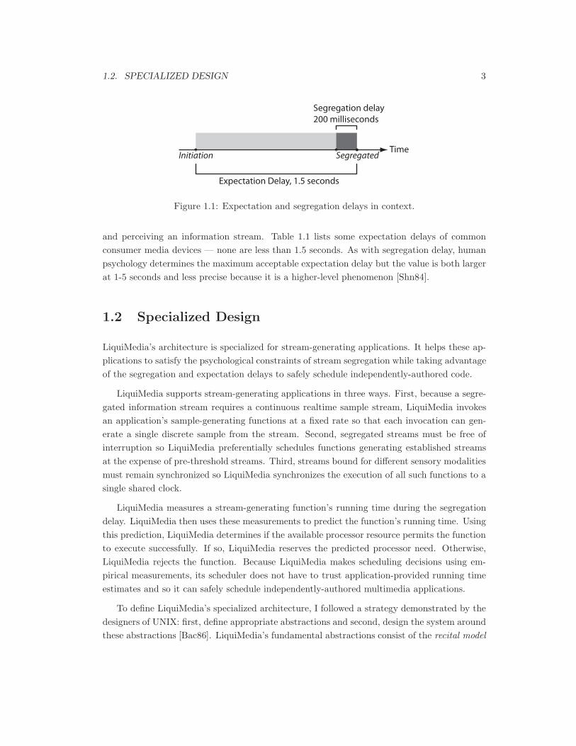
In addition to the segregation delay, a user’s experience with an information stream alsohas expectation delay. Figure 1.1 shows these two latencies in context. The expectation delayis the time that a user is willing to wait between activating (perhaps by pressing a button)
1Because human psychology determines the sampling rates needed for a satisfactory stream, exact lower
bounds do not exist [Har88, Han89]. I choose these particular values because most people notice the inferiority
of streams at lower sample rates.2McGrath and Summerfield conclude from their study of inter-modal relations of audio and vision in speech
understanding that 40 ms is an acceptable upper bound on the synchronization error between visual and
auditory streams of humans speaking [MS85]. Some streams require even tighter synchronization: Hirsh and
Sherrick showed that an observer can correctly determine the order of events occurring on different sensory
modalities down to intervals of only 20 ms [HS61].
1.2. SPECIALIZED DESIGN 3
Segregation delay200 milliseconds
Expectation Delay, 1.5 seconds
TimeInitiation Segregated
Figure 1.1: Expectation and segregation delays in context.
and perceiving an information stream. Table 1.1 lists some expectation delays of commonconsumer media devices — none are less than 1.5 seconds. As with segregation delay, humanpsychology determines the maximum acceptable expectation delay but the value is both largerat 1-5 seconds and less precise because it is a higher-level phenomenon [Shn84].
1.2 Specialized Design
LiquiMedia’s architecture is specialized for stream-generating applications. It helps these ap-plications to satisfy the psychological constraints of stream segregation while taking advantageof the segregation and expectation delays to safely schedule independently-authored code.
LiquiMedia supports stream-generating applications in three ways. First, because a segre-gated information stream requires a continuous realtime sample stream, LiquiMedia invokesan application’s sample-generating functions at a fixed rate so that each invocation can gen-erate a single discrete sample from the stream. Second, segregated streams must be free ofinterruption so LiquiMedia preferentially schedules functions generating established streamsat the expense of pre-threshold streams. Third, streams bound for different sensory modalitiesmust remain synchronized so LiquiMedia synchronizes the execution of all such functions to asingle shared clock.
LiquiMedia measures a stream-generating function’s running time during the segregationdelay. LiquiMedia then uses these measurements to predict the function’s running time. Usingthis prediction, LiquiMedia determines if the available processor resource permits the functionto execute successfully. If so, LiquiMedia reserves the predicted processor need. Otherwise,LiquiMedia rejects the function. Because LiquiMedia makes scheduling decisions using em-pirical measurements, its scheduler does not have to trust application-provided running timeestimates and so it can safely schedule independently-authored multimedia applications.
To define LiquiMedia’s specialized architecture, I followed a strategy demonstrated by thedesigners of UNIX: first, define appropriate abstractions and second, design the system aroundthese abstractions [Bac86]. LiquiMedia’s fundamental abstractions consist of the recital model
4 CHAPTER 1. INTRODUCTION
Information Streams
Composers Performers Audience
RealtimeNon-realtime
Conduits
Figure 1.2: Recital Model
and the architectural requirements embodied in LiquiMedia’s four design principles.
1.2.1 The Recital Model
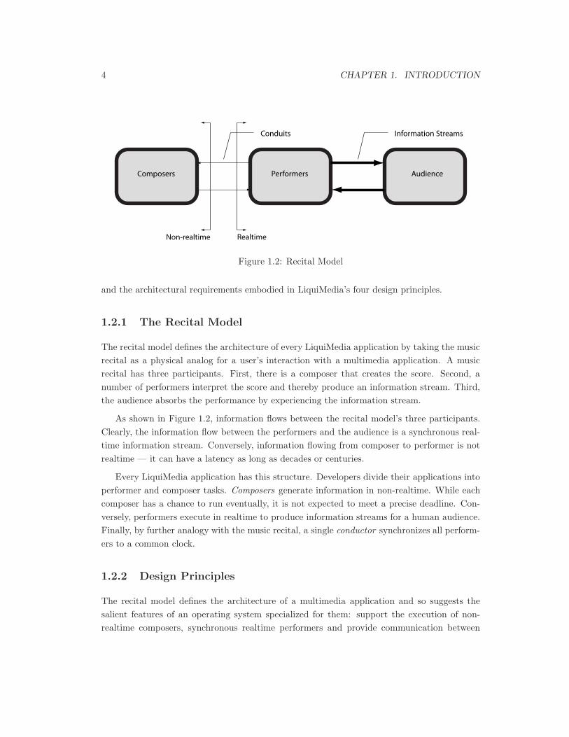
The recital model defines the architecture of every LiquiMedia application by taking the musicrecital as a physical analog for a user’s interaction with a multimedia application. A musicrecital has three participants. First, there is a composer that creates the score. Second, anumber of performers interpret the score and thereby produce an information stream. Third,the audience absorbs the performance by experiencing the information stream.
As shown in Figure 1.2, information flows between the recital model’s three participants.Clearly, the information flow between the performers and the audience is a synchronous real-time information stream. Conversely, information flowing from composer to performer is notrealtime — it can have a latency as long as decades or centuries.
Every LiquiMedia application has this structure. Developers divide their applications intoperformer and composer tasks. Composers generate information in non-realtime. While eachcomposer has a chance to run eventually, it is not expected to meet a precise deadline. Con-versely, performers execute in realtime to produce information streams for a human audience.Finally, by further analogy with the music recital, a single conductor synchronizes all perform-ers to a common clock.
1.2.2 Design Principles
The recital model defines the architecture of a multimedia application and so suggests thesalient features of an operating system specialized for them: support the execution of non-realtime composers, synchronous realtime performers and provide communication between

1.2. SPECIALIZED DESIGN 5
them. However these suggestions remain too vague to guide the design of an operating system.Consequently, I augmented the recital model with four principles: the principle of partitioning,synchronous execution, modularity and ultra-fine granularity realtime. These four principlesformalize a multimedia operating system’s support for recital-model applications generatingpsychologically satisfactory streams.
1.2.2.1 Processor Partitioning
The principle of processor partitioning enables the recital model of a multimedia application.It requires application developers to divide applications into performers and composers whileimposing the commensurate requirement on the operating system — that it execute these twokinds of tasks. In particular, the principle of processor partitioning demands three things:operating system support for executing composers and performers from different applications,a mechanism for them to communicate and finally an architecture that precludes the composersfrom ever jeopardizing the realtime execution of performers.
Why does LiquiMedia require application developers to adopt the recital model architec-ture for multimedia applications? The recital model and hence the principle of processorpartitioning helps application developers in two ways.
First, it requires developers to consider what parts of an application have realtime con-straints and which parts do not. Due consideration to this division improves an application’sreliability by providing access to realtime scheduling without forcing the difficulties of realtimedevelopment on the entire application.
The alternatives are both bad: application developers can either use only non-realtimetasks or convert the entire application to run in realtime. The first choice precludes reliablegeneration of information streams. The second choice forces the difficulties of realtime devel-opment noted by Wirth [Wir77] on even the non-realtime portions of the application. Becauserealtime development is harder than non-realtime development, minimizing the amount ofrealtime code in an application simplifies its development.
Second, requiring developers to expose the division inside their application between realtimeand non-realtime execution exposes more of an application’s structure to the operating system.The LiquiMedia scheduler uses this exposed structure to better schedule the performers of allapplications.
These two advantages are lost if developers reject the recital model with the excuse thatits adoption is “too much effort”. Consequently, the principle of processor partitioning re-quires the operating system to provide easy-to-use primitives for the creation, scheduling andcommunication between composer and performer tasks.

6 CHAPTER 1. INTRODUCTION
1.2.2.2 Synchronous Execution
The principle of synchronous execution formalizes three requirements of successful informationstream generation on a computer system. First, as Abadi and Lamport [AL92] observed, acomputer system generates a realtime information stream by emitting a sequence of discretesamples at a constant and sufficiently rapid rate that the samples appear continuous. Sec-ond, once the stream’s age exceeds the segregation delay, the computer system must continueto generate the samples until the stream’s natural end. Third, the computer system mustsynchronize all the generated streams with one another.
Given that performers generate all realtime information streams in the recital model, theserequirements can be re-expressed more precisely. First, each invocation of a performer gen-erates a single sample in the stream. Every basic period, the LiquiMedia conductor invokesall scheduled3 performers and thereby, over a number of basic periods, generates the sequenceof discrete samples that comprise a stream as described by Abadi and Lamport [AL92] andin the digital signal processing literature [OS94]. For example, the LiquiMedia prototype be-gins a new basic period on each video retrace interrupt — every 13ms — and hence invokesperformers at a rate ideal for generating information streams for the visual modality.4
Second, the principle requires continuous and predictable execution: once the conductorhas invoked a performer, it continues to execute that performer in all subsequent basic periodsunless the performer encounters an error or requests its removal from the schedule. This“inertial” property of a performer permits it to generate psychologically continuous streams.In particular, the conductor must preserve established streams at the expense of pre-thresholdstreams by preferentially executing the performers generating established streams. Further,predictable execution requires that the conductor executes each application’s performers inthe order specified by the application.
Third, the principle requires that the conductor executes all performers from a commonrealtime clock and thereby synchronizes all generated streams. Moreover, this clock’s periodmust be less than the 20 ms limit discovered by Hirsh and Sherrick to ensure that performersexecuted in the same basic period always appear synchronized [HS61]. While this approachguarantees synchronized streams, it does require developers to correct for possible mismatchesbetween a stream’s natural period and the conductor’s basic period. For example, the durationof the LiquiMedia prototype’s basic period contains a non-integral number of CD-quality audiosamples so an audio-generating performer must appropriately adjust the number of samplesthat it produces in each invocation.
3This description assumes a simple schedule. Otherwise, the conductor executes all performers on a single
schedule path as described in Section 4.8 and Section B.3.3.4This choice of basic period does not preclude the generation of audio streams — a performer generating
an audio stream produces 13ms of audio samples in each invocation. Synchronizing audio to a video clock is
reasonable given the dominance of the visual modality in people [BR81].

1.2. SPECIALIZED DESIGN 7
1.2.2.3 Modularity
The principle of modularity requires LiquiMedia to safely execute multiple independently-authored applications. However the principle goes far beyond this requirement by also support-ing the composition of multimedia applications from multiple independently-authored modules.In particular, the principle requires that the operating system can continue to execute cor-rect performers in realtime despite attempting the execution of an incorrect or even maliciousperformer.
Three reasons justify the inclusion of the principle. First, computers have operating systemsto distribute resources including, most importantly, the processor over a dynamic selection oftasks. A multimedia operating system exists for the same reason: to distribute resourcesbetween tasks that generate multiple information streams.
Second, realtime scheduling should be available to unprivileged applications. All multime-dia applications, regardless of their authorship, need realtime scheduling for their performersif they are to successfully generate information streams. For example, Solaris offers both real-time and non-realtime schedulers. However because only root-privileged processes can use therealtime scheduling facilities, sensible system security policies preclude most multimedia appli-cations such as interactive video games from using them. Similarly, cellular phones have hardrealtime operating systems but force downloaded video games to execute in a non-realtime Javavirtual machine. In both examples, realtime scheduling is available only to privileged applica-tions because its misuse can easily crash the operating system.5 The principle of modularitytherefore requires that LiquiMedia can safely enforce allocations of processor to performersregardless of their origin and behaviour.
Third, the principle extends the benefits of modular object-oriented development to multi-media applications. Non-realtime software architectures such as Andrew, JavaBeans and COM,have shown that assembling applications from existing independently-authored modules greatlyspeeds and simplifies implementation of feature-rich applications [Bor90, Sun00, Mic00b].
The DirectShow and Java Media Framework (JMF) stream-generating frameworks basedon COM and JavaBeans respectively show that the rapid development advantages of mod-ular software extend to multimedia applications as well. However, while these frameworkssupport the combination of independently-authored components, neither framework executesthese components in realtime [Mic00a, Jav00].6 In combining independently-authored real-time performers in a single application, as required by the principle of modularity, LiquiMediasurpasses these modular frameworks.
5During LiquiMedia’s development, simple programming errors regularly crashed the system.6Windows 2000 provides a DirectShow facility called kernel streaming drivers where an information stream
generating component runs at high priority inside the NT kernel [DN99]. This facility is obviously only available
to privileged applications and its use entails the inconvenience of coding a device driver.
8 CHAPTER 1. INTRODUCTION
1.2.2.4 Ultra-fine Granularity
The principle of ultra-fine granularity requires that LiquiMedia can efficiently execute largenumbers of performers such as sprite or filter functions whose execution times range fromten to a thousand microseconds. The principle is essential for two reasons. First, there willbe many performers. Second, each one will be invoked many times. The principle thereforedemands the smallest possible overhead on each performer invocation so as to make efficientuse of processor resources.
LiquiMedia executes many performers because of the principle of modularity. The princi-ple of modularity facilitates application development by executing applications composed ofseparate modules. As the example in Section 4.8 shows, even a simple video player applicationcan contain eleven performers and modular frameworks for video decoding require more. Amulti-party video conferencing application hosting four participants requires replicating thevideo player’s eleven performers three times and adds more performers for video and audiocapture. Such an application uses upward of forty performers.
LiquiMedia invokes these performers many times to satisfy the principle of synchronousexecution. LiquiMedia must dispatch each performer once per basic period. At the 76Hz basicperiod rate of the prototype, the video conferencing application requires 3040 performer acti-vations per second. At these rates, only the inexpensive invocations required by the principlepermit efficient operation.
1.3 Applications
An implementation of LiquiMedia’s four fundamental design principles has numerous practicalbenefits. For example, LiquiMedia’s ability to execute and synchronize independently-authoredmultimedia applications enables the development of modular media-rich user interfaces whilepartitioned realtime and non-realtime tasks can reduce the hardware costs of some multimediadevices. The examples in the remainder of this section further illustrate the advantages ofhaving the architectural features embodied in the four principles.
1.3.1 On the Desktop
Traditional desktop machines have for several years reached a level of hardware performancethat supports multiprocessing time-shared operating systems such as UNIX or Windows NT.With increasing clock speeds and instruction set extensions such as MMX, streaming SIMD andVIS, desktop machines can now easily deliver sufficient operations per second to simultaneouslygenerate many realtime information streams [Sun95a, Int99, SPE95].

1.3. APPLICATIONS 9
However, despite abundant processor resources, scheduling failures continue to disruptestablished information streams generated by traditional desktop operating systems.7 Rea-sons for these failures include non-preemptible kernel code blocking the execution of stream-generating functions, overly long task quanta and virtual memory systems purging a stream-generating function’s pages.8 Further, even when a desktop operating system, such as Solarisor IRIX, actually provides realtime scheduling, it permits only specially privileged applica-tions to execute in realtime [KSSR96, Sun95c]. These operating systems exclude un-privilegedapplications because they provide neither processor reservation nor a mechanism for enforcingprocessor reservation.
In contrast, LiquiMedia can safely schedule even untrusted independently-authored appli-cations. Providing realtime execution to untrusted applications like audio players and gamespermits them to run free of scheduling glitches. Universal availability of realtime services alsopermits augmenting the primarily static textual content of most modern user interfaces withcontinuous sounds, animation and even haptic feedback.
For example, realtime fragments from different applications could cooperate to generateinformation-bearing sound consisting of multiple streams of sound. In my Master’s thesis, Ishowed that a human user can more effectively perform a foreground task requiring the visualmodality if information that the subject must simultaneously monitor is presented as streamsof sound [Kro93]. Combining information-bearing sound and video streams from differentapplications requires an operating system capable of synchronizing multiple independently-authored realtime fragments at the latencies needed for controlling motor coordination.
Smoothly time-varying visuals have the potential to enhance an application.9 For example,an application can generate additional brightness levels by alternating between the two closesthardware pixel values in every frame. However, generating additional brightness levels in thisfashion requires reliable hard realtime [Cor70]. Further, as soon as another application tries touse this technique to display additional brightness levels, the operating system must supportindependently-authored realtime fragments.
Lastly, consider, a window system equipped with a force feedback pointing device. Eachapplication both draws content on the screen outlining buttons, selection handles or text andgenerates small resistances as the user moves the pointing device over visible objects. Dulatshowed the potential of a simulated force feedback component in improving user accuracy andspeed [Dul01]. A window system making general use of this scheme needs to simultaneouslyexecute a small force feedback information stream generator for every application and keep
7See Appendix C for a summary of a simple experiment conducted on the author’s desktop machine that
shows scheduling failures even with very powerful hardware and a low-utilization stream generation task.8For example, traditional UNIX kernels were non-preemptible [Bac86].9Note that the “Aqua” user interface for MacOS X includes significant animation elements that show a
trend toward increased use of time-varying visual elements in a user interface [App00a]. Also, Microsoft has
produced a program for the generation of time-varying “rich” content [Mic00c].

10 CHAPTER 1. INTRODUCTION
these streams synchronized with mouse pointer movement. Such a window system requiresrealtime scheduling available to independently-authored applications.
The stream-generating tasks described in the above examples all share the same threecharacteristics. First, each task only requires a small amount of processor time. Second, eachtask executes repeatedly. Third, the tasks have tight time constraints. These are the featuresrequired by the principles of modularity, synchronous execution and ultra-fine granularity,making LiquiMedia ideally suited for all of these applications.
The specialized design embodied in the four principles also enables complex interfacesconsisting of multiple information streams such as the following scenario [Kro99]. As withthe examples above, the applications in this example are independently-authored and containmultiple small, synchronous realtime stream-generating tasks.
As an example, consider the experience of a consumer of Internet-provided ser-vices. Suppose he is watching a football game on television. In the dead time be-tween plays, he uses a football interpreter/simulator which was downloaded to hismedia appliance, to re-run in a second window of his high definition television, por-tions of the already-played game, inputting different plays, blocking assignments,and pass coverage, to see what might have happened. At this point the Internettelephone rings. When he accepts the call, the avatar of an acquaintance living inNew Orleans appears on the screen in a third window. He chooses an avatar toappear on the caller’s display, connecting its facial expressions to his own face asinterpreted from real-time captured video. The avatar’s audio output will be theuser’s voice, and forces sensed on the user’s game controller provide force-feedbackon the caller’s game controller, enabling virtual handshaking and back-slapping.The caller, it turns out, has noticed that our user is playing the same footballsimulator and wants to play in two-player mode, each second-guessing the choicesof a different team and replaying the game through the simulator. Once acceptingthe suggestion of two way play, the user shrinks the call window to a size suitablefor kibitzing and the the simulator shifts into two-player mode. Life goes on.
This scenario is not an unreasonable use of a media appliance. We will examinethe requirements needed to bring it to fruition. First, from the user’s viewpoint,enjoying a football game in the manner discussed above requires little additionallearning. A user would have to use the football simulator interface, social protocolsfor virtual handshaking, and so on. These are easy compared to the new habitsrequired when users started using telephones or automobiles and will seem secondnature to the people who play network games now.
Second, this scenario requires immense amounts of computation and commu-nications bandwidth. As for computational power, machines such as the NextGeneration PlayStation and the even more powerful hardware that will follow have
1.3. APPLICATIONS 11
the processing power needed. Cable modems or DSL satisfy the scenario’s need forcommunications bandwidth.
Third, the scenario depends on rapid advances in application software. Ata minimum, the software must interpret the football game and the live video ofthe user and his caller, simulate the complex interactions of twenty-four10 footballplayers and integrate input from two sources into a distributed simulation. Butapplication software is the fastest progressing part of the computer industry andits only limitation seems to be knowing what to provide. Already, early versions ofsome of the required application software exist in multi-player Internet games andsports simulation games.
However, with the fourth requirement, we will see how LiquiOS [a LiquiMedia-architecture operating system] is indispensable to enabling the scenario describedabove. In the above scenario, a single media appliance executes a football sim-ulator, a video player, an Internet video phone and an animated avatar. Thesevarious applications, authored in different ways by different firms must cooperatein realtime on a single system, all sharing various data sources over which theyhave little or no control.
This combination of software faces difficult realtime constraints. The softwarecan tolerate some temporal faults if they result in only almost imperceptible glitchesin the audio or animation while other faults such as un-synchronized audio andvideo will make the overall system unsaleable. Furthermore, while the system asa whole can call on the user for help in allocating resources, if it needs too muchhelp, the system is once again unsaleable.
Only an operating system that satisfies the principles of partitioning, synchronous ex-ecution, modularity and ultra-fine realtime can enable the user interfaces discussed above.Developers can use the LiquiMedia architecture to add these features to existing desktop andembedded operating systems.
1.3.2 The Embedded Space
The architectural features required by the principle of processor partitioning can, when com-bined with the other principles, also enable hardware cost savings. It has become common fordevices aimed at the consumer electronics market that execute a mixture of non-realtime tasksand stream-generating tasks to have separate physical processors for the two types of tasks.
While dividing tasks between processors in this way ensure that tasks from different schedul-ing classes cannot mutually interfere, its rigidity wastes resources when processor loadings do
10The game called football has significant regional difference in rules. This example assumes American
football.
12 CHAPTER 1. INTRODUCTION
Multi-processor Settop Single Processor Settop
Video
Sound Admin
General Purpose�Processor
Figure 1.3: Replacing hardware partitioning with software partitioning can lower overall systemcosts.
not correspond to their design-time scaling. For example, some Nokia cellular phones confineall user interface processing to one of two identical processors because the second one is re-served for realtime tasks such as voice compression [Wel99]. As a result, playing a game onthe phone leaves the second processor entirely idle.11
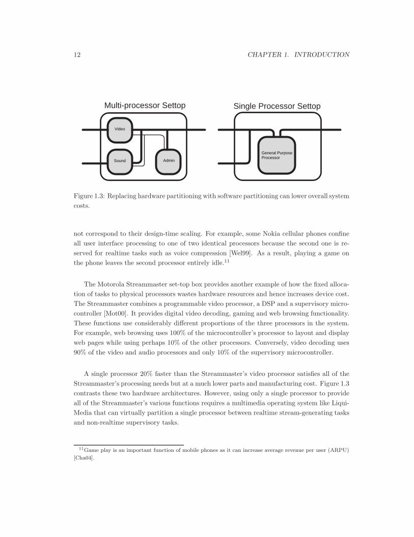
The Motorola Streammaster set-top box provides another example of how the fixed alloca-tion of tasks to physical processors wastes hardware resources and hence increases device cost.The Streammaster combines a programmable video processor, a DSP and a supervisory micro-controller [Mot00]. It provides digital video decoding, gaming and web browsing functionality.These functions use considerably different proportions of the three processors in the system.For example, web browsing uses 100% of the microcontroller’s processor to layout and displayweb pages while using perhaps 10% of the other processors. Conversely, video decoding uses90% of the video and audio processors and only 10% of the supervisory microcontroller.
A single processor 20% faster than the Streammaster’s video processor satisfies all of theStreammaster’s processing needs but at a much lower parts and manufacturing cost. Figure 1.3contrasts these two hardware architectures. However, using only a single processor to provideall of the Streammaster’s various functions requires a multimedia operating system like Liqui-Media that can virtually partition a single processor between realtime stream-generating tasksand non-realtime supervisory tasks.
11Game play is an important function of mobile phones as it can increase average revenue per user (ARPU)
[Cha04].
1.4. LIQUIMEDIA OVERVIEW 13
1.4 LiquiMedia Overview
LiquiMedia’s architecture follows naturally from the recital model and the four design prin-ciples. As required by the principle or partitioning, LiquiMedia has composer and performertasks. An IPC mechanism called a conduit connects these different kinds of tasks. Becausecomposers and performers differ, separate sets of operating system primitives support theirexecution.
Composers are preemptible threads of computation that can be transparently suspendedand restarted. In the LiquiMedia prototype, composer tasks are POSIX-style threads [Sun95b].
Performers are atomically executed functions. The conductor executes each scheduledperformer once per basic period and expects the performer to voluntarily return12 to theconductor once it has generated the current portion of an information stream. Performersare functions because [KC96] showed that the overhead of preemptive threads violates theprinciple of ultra-fine granularity.
The conductor executes performers from a schedule prepared by an asynchronous com-poser task called the scheduler. Having the conductor execute performers from a pre-preparedschedule has four advantages. First, it helps to satisfy the principle of synchronous realtime’s“inertial” property. Second, it simplifies LiquiMedia’s development by following Wirth’s rec-ommendation to minimize the quantity of code that must execute in realtime. Third, itminimizes the conductor’s per-performer invocation overhead by putting schedule preparationin a composer. Finally it improves system utilization as a whole by amortizing the cost ofpreparing a schedule over many basic periods.
LiquiMedia computes a probabilistic estimate of each performer’s running time and ad-mission-tests performers using this estimate. The combination of admission control and acontinually updated probabilistic estimate of a performer’s running time permits LiquiMedia toexecute independently-authored performers with a quantifiable probability of meeting realtimeguarantees.
LiquiMedia has two levels of admission control: lifetime and instantaneous. The schedulerperforms the lifetime context admission test as it prepares a new schedule for subsequent useby the conductor. The test consists of the scheduler verifying that an estimate of the totalrunning of all scheduled performers is less than the basic period. The conductor invokes theinstantaneous admission control test prior to invoking a performer. For each performer, itverifies that the time remaining in the basic period exceeds an estimate of the performer’srunning time.
Because both admission control mechanisms depend on statistical estimates of a performer’srunning time, they can fail. Consequently, LiquiMedia includes three techniques to address
12As discussed in Chapter 4, a performer that does not voluntarily return is incorrect and is removed from
the schedule.
14 CHAPTER 1. INTRODUCTION
admission control failure. First, the conductor hard limits the execution of any particularperformer with a watchdog timer firing at basic period boundaries. Second, the conductoruses its instantaneous context admission control mechanism to defer a performer’s executionto a subsequent basic period rather than having it interrupted by the start of the next basicperiod. Third, the scheduler regularly updates its estimates of each scheduled performer’srunning time from the collected measurements of recent performer invocations and repeats theaverage context admission control test on the entire schedule. Should the schedule becomeinadmissible, the scheduler corrects it such that performers generating established informationstreams continue to have the specified minimum probability of executing in realtime.
LiquiMedia’s admission control mechanisms require a priori knowledge of a performer’srunning time. LiquiMedia takes advantage of the properties of an information stream in twoways to predict a performer’s running time. First, because the continuity of an informationstream requires a performer to execute similar operations throughout the stream’s lifetime, aperformer’s past running times predict its future running times. Second, the segregation delayallows the combination of the conductor and scheduler to measure a performer’s running time,estimate its future running time and admission test it all before the human user segregates thenewly created stream.
Consequently, a user’s experience starting a LiquiMedia application such as a video playerconsists of invoking the player, pressing the play button, and after the expectation delay haselapsed, either seeing smooth video playback or a dialog indicating that the application cannotobtain sufficient processor for its performers. Inside LiquiMedia, the user’s invocation actioncreates a new application as a single composer. When the user presses the play button, thiscomposer submits a schedule of performers to the LiquiMedia scheduler.13 The submittedperformers begin executing approximately 30ms later. If sufficient processor exists for theirexecution, they continue until the user presses the player’s stop button. Otherwise, ten basicperiods later (130 milliseconds in the prototype,) the scheduler determines that the performerscannot reliably continue. It then removes them from the schedule and notifies the originatingcomposer which communicates its regrets to the user in a dialog.
LiquiMedia’s empirical approach to determining a performer’s running time sacrifices theabsolute guarantees of hard realtime scheduling. However, this empirical approach is a goodcompromise that allows LiquiMedia to achieve the principle of modularity. LiquiMedia canprofile and admission-test performers within 160ms — under the segregation threshold of aninformation stream. Moreover, even once the performer has been admitted into the schedulebased on a probabilistic estimate of its running time, a human user will tolerate the occasionalglitches when it runs over its estimated running time.
Two other approaches exist for determining a performer’s running time in advance: de-veloper provided declarations and automatic determination. Neither approach can satisfy the
13This design choice is not ideal but simplifies the example.
1.5. ORGANIZATION 15
principle of modularity.
Developer-provided declarations cannot satisfy the principle because, whether through ma-chine dependency, error or malice, they cannot be trusted. For example, there is no incentivefor developers to expend significant effort14 computing an accurate bound on a performer’srunning time when a declaration of 0 running time will insure that the performer is not barredfrom the schedule for excessive resource usage. Moreover, a hardware difference, such as theprocessor cache size, between the developer’s and user’s machine can significantly change therunning time of these assembly instructions. Because this approach precludes the safe execu-tion of independently-authored performers, it cannot satisfy the principle.
Automatically determining a bound on a performer’s running time cannot satisfy the prin-ciple either because the determination is impossible. Automatically bounding a performer’srunning time requires knowing if it can complete and is hence is an insolvable instance ofthe halting problem [HU79]. The alternative is to restrict a performer to a regular-expressionequivalent subset of a general purpose programming language [LM95]. Given this reduction,mechanical techniques based on control-path chains, data-usage paths and integer optimiza-tion can be used to compute a worst case bound on a performer’s running time. However,as with developer declarations, to execute in finite time, mechanical reduction must trust thedeveloper to have confined his code to the acceptable language subset.
Automatic determination has at least two other practical problems. First, mechanicalestimation techniques produce overly pessimistic bounds because they ignore the performancebenefits of multi-level data caches, super-scalar architectures and speculative branch prediction[LHS+96, LMW96]. Second, automatic determination mechanisms require an understanding ofa performer’s code equivalent to a compiler’s internal representation of the original source-code.Given that commercial software vendors usually ship their applications compiled, an automaticdetermination mechanism capable of supporting independently-authored performers thereforerequires a decompiler.
1.5 Organization
The remainder of this thesis discusses LiquiMedia in greater detail. LiquiMedia is specializedfor the needs of multimedia applications. It takes advantage of the domain — generating infor-mation streams for a human audience — to provide unique capabilities in a novel fashion. Thefour design principles of processor partitioning, synchronous execution, modularity and ultra-fine granularity embody both the specialized requirements of information stream generatingapplications and the unique capabilities that this specialization permits.
14Counting assembly language instructions.

16 CHAPTER 1. INTRODUCTION
Chapter 3 discusses numerous other operating systems and media generation frameworkswhose function or approach overlaps LiquiMedia’s. Owing to their number and to furtherclarify LiquiMedia’s uniqueness of approach, I organized the systems presented in Chapter 3into the taxonomy of operating system design features defined in Chapter 2.
Chapter 4 defines the LiquiMedia architecture in greater detail than Section 1.4 while Ap-pendix B supplements Chapter 4 to a level of detail sufficient for reimplementation. Chapter 5discusses the implementation of the prototype while Chapter 6 presents an empirical valida-tion of the prototype’s ability to satisfy the fundamental design principles. Finally, Chapter 7discusses the future research suggested by the existing architecture and results.

Chapter 2
The RTOS Design Space
Chapter 1 introduced the LiquiMedia operating system for multimedia applications. LiquiMe-dia’s specialized architecture satisfies four fundamental principles of a multimedia operatingsystem: processor partitioning, synchronous realtime, modularity and ultra-fine granularity.LiquiMedia is unique in satisfying these principles. Furthermore, LiquiMedia satisfies theprinciples with a unique architecture.
Demonstrating the uniqueness of the LiquiMedia architecture requires comparing it toother realtime operating systems. However, as is demonstrated in Chapter 3, the multitude ofrealtime operating systems and multimedia frameworks makes this task difficult. Categorizingall of these systems by their dominant architectural features provides a structure for theexposition and facilitates comparing them to LiquiMedia. To do so, I devised a taxonomy forrealtime operating systems that categorizes them by their design aspects. The remainder ofthis chapter presents this taxonomy.
The taxonomy presented here organizes operating systems by their design aspects. A designaspect is a feature of an operating system’s design and is the result of an architectural choiceby the OS designer. Obviously, each operating system comprises multiple design aspects andthese determine its position in the taxonomy. The set of all possible design aspects form anoperating system design space.
A design space organizes design aspects by their relationships. I adopted the three relation-ships defined in Sima et al. [SFK97]: “consists of”, “exclusively performs”, and ”performs”.First, the consists of relationship indicates that a design aspect must contain each of the or-thogonal subordinate design aspects. For example the UNIX kernel consists of (among othercomponents) a file system and a scheduler. As demonstrated by the various research projectsbuilt around Linux, operating system implementors can vary these aspects independently[www00b, www00a].
17

18 CHAPTER 2. THE RTOS DESIGN SPACE
“consists of” – the design of A contains all of the orthogonal subordinate aspects in B and C
“exclusively performs” – the design of A uses one and only one of the subordinate aspects B and C
“performs” – the design or A uses some combination of the sub-ordinate aspects B and C
Description Diagrammatic Representation
A
A
B
B
C
C
A
B C
Figure 2.1: The three basic DS-Tree diagrammatic conventions.
Second, the exclusively performs relationship indicates that a design aspect can only beimplemented by one and only one of its subordinate aspects. For example, a UNIX kernel maybe single threaded (non-reentrant) or multi-threaded. Both together is not possible.
Third, the performs relationship indicates that a design aspect can be implemented bysome combination of its subordinate aspects. For example, a UNIX kernel may implement itsvirtual memory subsystem with swapping, paging or both.
Sima et al. defined a diagrammatic convention called design space trees (DS-trees) forrepresenting these relationships [SFK97]. Figure 2.1 shows the DS-tree graphical convention.DS-trees make visual the inter-dependencies between design aspects including orthogonal orexclusive relationships. DS-trees have been used extensively to illustrate design spaces [Bar76,Bar77, BS73, Bar93, BN70, BN71].
2.1 Taxonomy Overview
Because this thesis is concerned with operating system support for multimedia applications,the taxonomy presented in this chapter concentrates on those design aspects relevant to theexecution of independently-authored realtime applications and ignores unrelated operatingsystem design aspects such as name space management or storage.

2.1. TAXONOMY OVERVIEW 19
Statistical
Declarative
Absent
Admission Controlon
Hardware
Task
HierarchicalMechanismnis
Impermeable
Permeable
Permeabilityabil
Partitioning
Static Priority
Rate-Based
EDF
Distributed
Schedulingngng
Mutexes
Synchronous Message Passing
Divisible Taske Ta
Asynchronous Message Passing
Linked Fragments
Atomic Taskc Ta
IPC
RealtimeOperating System
Design Space
Event-triggered
Externalizationzat
Global
Per-task
Time-triggeredgge
Preemptive Threads
Non-preemptive Threads
Task Abstractionrac
Fixed
Adaptive
Performersme
Hard Realtime
Deadline SensitivityensenExtension
Incomplete
Soft Realtimealt
Figure 2.2: The figure shows the complete RTOS design space. An operating system consistsof one (sometimes more) design aspect leaf from from each of the “consists-of” relationshipsin the figure.

20 CHAPTER 2. THE RTOS DESIGN SPACE
Subject Requires Precludes
Hard RealtimeDeadline Sensitivity
one of: StaticPriority Scheduling,EDF Scheduling,DistributedScheduling
StatisticalAdmission Controlor Rate-basedScheduling
Static PriorityScheduling
Preemptive Threadsand Time-triggeredexternalization
Performers andNon-preemptiveThreads
EDF Preemptive Threads Performers andNon-preemptiveThreads
Rate-basedScheduling
Preemptive Threads Hard realtimedeadline sensitivity,Performers andNon-preemptiveThreads
StatisticalAdmission Control
Hard RealtimeDeadline Sensitivity
Impermeablepartitioning andTask partitioning
PreemptiveThreading
Divisible Task IPC
Divisible Task IPC Preemptive Threadsor Non-preemptiveThreads
Performers
Table 2.1: The table shows some relationships between different design aspects. The Subjectcolumn contains the subject aspects. The Requires column contains design aspects which thesubject requires while the Precludes column contains aspects incompatible with the subject.
Figure 2.2 shows the complete design space. At the highest level, it contains seven top-leveldesign aspects linked by the “consists of” relationship: task abstraction, deadline sensitivity,externalization, scheduling, partitioning, admission control and inter-process communication(IPC). The partitioning aspect contains two “consists of” sub-aspects: permeability and thepartitioning mechanism.
The design space further divides each of these eight aspects into sub-aspects that haveeither the “exclusively performs” or “performs” relationship. Every operating system combinesone leaf design aspect from each “exclusively performs” relationship and one or more designaspects from each “performs” relationship. For example, a cyclic executive like the Virtuoso

2.2. TASK ABSTRACTION 21
Timerp,i
tp,i,1 tp,i,2 tp,i,3
dp,i
Figure 2.3: Threaded task abstractions permit sub-dividing a task’s execution into multipleslices in the interval between its release and deadline.
OS for digital signal processors has global time-triggered externalization, fixed performer task-abstraction, distributed scheduling, permeable task partitioning, absent admission control,atomic IPC and hard realtime deadline sensitivity [Inc00a].
While all possible operating systems map to some combination of leaf design aspects,not all arbitrary combinations of design aspects are valid operating systems. For example,the indivisible performer task abstraction excludes the divisible task IPC aspect. Table 2.1summarizes some of these additional constraints.
2.2 Task Abstraction
This design space assumes that an operating system supports multiple tasks and so mustprovide a task abstraction. A task abstracts a von Neumann machine: each task combinescode and state and has exclusive use of the processing hardware while it is executing. Theoperating system controls the execution order of tasks. Typically it chooses an order thatgives the outward appearance of many tasks executing simultaneously. The task abstractionhas three sub-aspects with a “performs” relationship: performers, preemptive threading andnon-preemptive threading. These task abstractions differ in when they permit the operatingsystem to choose a different task to execute and the overhead required to switch between them.
Before discussing each of these sub-aspects individually, some mathematical preliminariesare necessary to formalize tasks and realtime execution. A realtime task has constraints onwhen it executes. Each task p has a sequence of release times and corresponding deadlines. Thei-th release of task p has release rp,i and deadline dp,i. Realtime execution of p requires its i-thexecution happen entirely within the interval [rp,i, dp,i). The application of p determines thevalues of all rp,i and dp,i. For example, an (un-buffered progressive scan) NTSC video playerhas a a sequence of releases at the start of the NTSC vertical retrace with correspondingdeadlines at the end of the vertical retrace and a 33.3ms interval between successive releases.
A threaded task abstraction, by definition, permits the operating system to divide taskexecution into slices.1 The tuple (p, i, j) uniquely identifies slice j of task p in release i. The
1The concept of a “slice” has no consistent name in the literature as “job”, “event” and “slice” all find use.
This thesis uses “slice”.

22 CHAPTER 2. THE RTOS DESIGN SPACE
Timer1,i
t1,i,1 t1,i,2 t1,i,3
d1,ir2,i d2,i
t2,i,1 t2,i,2
Figure 2.4: The interleaving of multiple slices of multiple tasks provides the appearance, at asufficiently large time scale, of many tasks progressing in parallel.
operating system executes slice (p, i, j) atomically in time tp,i,j . Figure 2.3 shows an examplewhere the operating system has divided the execution of the i-th release of task p into threeslices. In this example, p has also successfully executed in realtime because its three slicesoccur entirely between rp,i and dp,i.
As shown in Figure 2.4, the operating system can provide the appearance of two moretasks executing simultaneously by interleaving the execution of slices comprising differenttasks. Over the time interval [r1,i, d1,i), tasks 1 and 2 compute results simultaneously. Thefiner the granularity of the task slices, the shorter the interval over which computation appearsto proceed in parallel. However, switching between slices (frequently called a context switch)itself consumes processor resources: wf when the task abstraction permits the OS to imposethe switch and wv when context switches occur only when the task voluntarily relinquishesthe processor. Necessarily, wv is less than or equal to wf ; often wv is much less than wf .
2.2.1 Performers
In the performer task abstraction, there are no slices. Instead, for each release i, the operatingsystem executes the entire task p without preemption. To insure that performers executewithout being preempted, they cannot use the divisible task IPC mechanisms discussed inSection 2.8.
Atomic execution has two related benefits. First, performers have the lowest context switchoverhead because context switches between performers are voluntary and occur only at theirend. Second, it is trivial to implement the context switch mechanism between performers astypically an assembly language return statement suffices.
However, these benefits have a price. For the operating system to successfully interleavethe execution of many applications such that they appear to execute in realtime, applicationdevelopers must divide applications into performers with sufficiently short running times. Two“exclusively-performs” sub-aspects indicate the mechanism used to specify “sufficiently short”execution time: fixed and adaptive.
In the fixed execution aspect, the performer’s running time is accepted as a given by theadmission control mechanism (discussed in Section 2.6), which releases the performer if its
2.2. TASK ABSTRACTION 23
estimate of the performer’s running time is less than the time available for the performer’sexecution. Conversely, in the adaptive execution aspect, application developers must write theperformer so that it limits its running time to an upper bound computed by the admissioncontrol mechanism and provided to the performer prior to its release.
2.2.2 Preemptive Threads
A preemptive thread is a task abstraction where the operating system provides each task withthe illusion of having the entire processor to itself. The operating system provides this illusionto many tasks by dividing them into slices and interleaving the execution of the slices.
Two features differentiate the preemptive thread design aspect from the other two taskabstractions. First, the division of a preemptive thread p into slices is completely invisibleto p except with respect to the passage of external time. Second, the operating system hascomplete control of the duration tp,i,j of each slice.
Making the boundaries between slices invisible to a preemptive thread requires a contextswitching mechanism that completely preserves the state of a thread at the end of each sliceand substitutes the previously saved state of a different thread. The time needed for a contextswitch bounds the performance of an RTOS using preemptive threading.
From the internal perspective of a preemptive thread, its assembly language instructionsexecute sequentially without interruption. However, the operating system can insert an ar-bitrary delay between any two successive instructions. Consequently, a preemptive threadexecutes decoupled from an external clock.
This decoupling greatly simplifies the implementation of non-realtime tasks: they run untilcomplete without consideration of the elapsed time. This feature is however inappropriate fora realtime task because it must be, by definition, bound to an external clock. Consequently, anRTOS using preemptive threads, having implemented a task abstraction that decouples taskexecution from external clocks, must add back in a mechanism that can synchronize differentthreads with external clocks. Such a mechanism both weakens the power of the preemptivethread abstraction and exposes the RTOS to the dangers of priority inversions.
2.2.3 Non-preemptive Threads
Non-preemptive threads occupy a middle ground between preemptive threads and performers.An operating system using the non-preemptive threads transparently interleaves the executionof slices of different tasks. However, the threads themselves specify at what points the operatingsystem may divide up their execution into slices.
Requiring the task to specify these division points has two advantages. First, the operatingsystem can use a simpler context switching mechanism when slices explicitly relinquish the

24 CHAPTER 2. THE RTOS DESIGN SPACE
Weakly Coupled
Strongly Coupled
DivisibleAtomic
PerformersNon-preemptive Threads
Preemptive Threads
Figure 2.5: The diagram shows how the three different task abstractions differ in two axes:divisibility and coupling.
processor. Second, application developers can obtain atomic execution of a code section simplyby omitting division points from the section.
However, non-preemptive threads place the operating system’s ability to multi-task at themercy of application developers because malicious code can omit division points. As a result,non-preemptive threads preclude satisfying the principle of modularity. Further, the inclusionof division points complicates the development of well-behaved applications as developers mustbe aware of the running time of each indivisible section.
In summary and as shown in Figure 2.5, the three different task abstractions differ in twoaxes: the divisibility of the task and its coupling to external time. Performers, by virtue oftheir atomic execution, are indivisible and totally coupled. Non-preemptive threads have someapplication-specified number of divisions and are coupled only within each division. Preemptivethreads are arbitrarily divisible into slices and are not intrinsically coupled to realtime.
2.3 Deadline Sensitivity
Correct execution of a realtime task requires that the operating system completes execution ofthe task before its deadline. Formally, in a release i, the operating system must execute taskp entirely within the interval [rp,i, dp,i). The values rp,i and dp,i are from a perfect realtimeexternal clock. Deadline sensitivity has two “exclusively-performs” sub-aspects: hard realtimeand soft realtime.
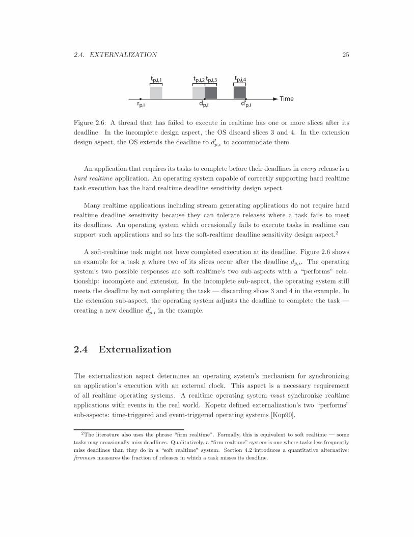
2.4. EXTERNALIZATION 25
Timerp,i
tp,i,1 tp,i,2 tp,i,3
dp,i d'p,i
tp,i,4
Figure 2.6: A thread that has failed to execute in realtime has one or more slices after itsdeadline. In the incomplete design aspect, the OS discard slices 3 and 4. In the extensiondesign aspect, the OS extends the deadline to d′p,i to accommodate them.
An application that requires its tasks to complete before their deadlines in every release is ahard realtime application. An operating system capable of correctly supporting hard realtimetask execution has the hard realtime deadline sensitivity design aspect.
Many realtime applications including stream generating applications do not require hardrealtime deadline sensitivity because they can tolerate releases where a task fails to meetits deadlines. An operating system which occasionally fails to execute tasks in realtime cansupport such applications and so has the soft-realtime deadline sensitivity design aspect.2
A soft-realtime task might not have completed execution at its deadline. Figure 2.6 showsan example for a task p where two of its slices occur after the deadline dp,i. The operatingsystem’s two possible responses are soft-realtime’s two sub-aspects with a “performs” rela-tionship: incomplete and extension. In the incomplete sub-aspect, the operating system stillmeets the deadline by not completing the task — discarding slices 3 and 4 in the example. Inthe extension sub-aspect, the operating system adjusts the deadline to complete the task —creating a new deadline d′p,i in the example.
2.4 Externalization
The externalization aspect determines an operating system’s mechanism for synchronizingan application’s execution with an external clock. This aspect is a necessary requirementof all realtime operating systems. A realtime operating system must synchronize realtimeapplications with events in the real world. Kopetz defined externalization’s two “performs”sub-aspects: time-triggered and event-triggered operating systems [Kop90].
2The literature also uses the phrase “firm realtime”. Formally, this is equivalent to soft realtime — some
tasks may occasionally miss deadlines. Qualitatively, a “firm realtime” system is one where tasks less frequently
miss deadlines than they do in a “soft realtime” system. Section 4.2 introduces a quantitative alternative:
firmness measures the fraction of releases in which a task misses its deadline.
26 CHAPTER 2. THE RTOS DESIGN SPACE
2.4.1 Time-Triggered
A task p in a time-triggered OS has a sequence of periodic releases with period TB:
rp,1, rp,1 + TB, . . . , rp,1 + iTB, . . .
and a deadline at the next release: dp,i = rp,i+1. A time-triggered operating system’s keyperformance metric is period size: the shortest TB that the operating system can support.
A time-triggered operating system has two subordinate design aspects with the “exclusively-performs” relationship: global period or per-task periods. In the global period design aspect,all tasks have the same period TB. In the per-application design aspect, each task p mayhave an different period d′p. A fixed global period such as found in a cyclic executive likeVirtuoso simplifies the operating system and significantly reduces the need for inter-task syn-chronization [Inc00a]. The per-application periods found in rate monotonic operating systemslike VxWorks have opposite advantages: simpler application development, more complicatedoperating system development and trickier synchronization [Win00].
2.4.2 Event-Triggered
An event-triggered operating system releases a task each time a previously-specified eventoccurs. As a consequence, an event-triggered RTOS has aperiodic release times rp,1, rp,2 . . ..The time between the i-th external event and the corresponding release rp,i is called thesystem’s latency and is an event-triggered operating system’s most important performancemetric.
These two mechanisms for externalizing an operating system have complementary strengthsand weaknesses. A time-triggered operating system is immune to event overload because itsapplications poll external sensors. Conversely, it wastes processor resources when it invokestasks in the absence of changes in sensor values.
An event-triggered operating system eliminates this waste by invoking applications onlywhen necessary. However, it can be overloaded by a burst of events.3 Consequently, time-triggered operating systems are preferable when applications interact with continuously chang-ing external sensors, generate continuously varying information streams or provide periodicoutput. Event-triggered operating systems are preferable when an operating system needs toefficiently handle events arriving at variable rates.
These two design aspects are not exclusive — a single RTOS can provide both external-izations. For example, hardware timer events in an event-triggered RTOS provide tasks withtime-triggered externalization. Conversely, a time-triggered RTOS can poll sensors and queuetasks for execution upon discovering changes in the value of the sensors.
3Hence requiring one of the admission control mechanisms discussed in Section 2.6.

2.5. SCHEDULING 27
2.5 Scheduling
An RTOS exists to allocate resources, particularly processor resources, to tasks.4 Conse-quently, the RTOS has a scheduler that allocates processor resources to tasks by controllingthe order of task execution and the running time of task slices. A good scheduling algorithm isindispensable in building an efficient and practical operating system. Consequently, researchershave extensively explored scheduling algorithms.
Scheduling algorithms naturally sub-divide into three separate design aspects linked by a“consists of” relationship: the scheduling function, admission control and partitioning. Underthis division, the scheduling function chooses the next task to be executed, admission controldetermines if a task can complete before its deadline and partitioning protects each task fromerrors or scheduling failures in other tasks.
These three design aspects are closely related. As a result, an actual scheduler implemen-tation has some fixed combination of sub-aspects chosen from each of these three aspects. Forexample, the popular rate monotonic scheduling (RMS) algorithm has no admission control,static priority scheduling and impermeable task partitioning [LL73].
The remainder of this section discusses scheduling functions while admission control isdiscussed in Section 2.6 and partitioning in Section 2.7.
The scheduling function S takes some portion of the operating system’s internal state asits arguments and returns a next task from P . Scheduling has four sub-aspects with the“exclusively-performs” relationship: static priority, EDF, rate-based and distributed schedul-ing. The first three of these, static priority, earliest deadline first (EDF) and rate-basedscheduling, have an algorithmic implementation of the function S. However, S can also alwaysbe represented by a set of of six-tuples {(p, i, j; q, k, l), . . .}, where an element (p, i, j; q, k, l)specifies that the operating system executes slice (q, k, l) of task q at the end of slice (p, i, j).5
If the set of tasks P is fixed and the operating system periodic, then the set definition of S isfinite.6
When the set representation of S is finite, it is a practical foundation for implementing anoperating system’s scheduling function for three reasons. First, the implementation runs inO(1) time and has a small constant. For example, a cyclic executive stores the set representa-tion of S in its program structure and so can choose the next task in a single assembly languageinstruction. Second, an RTOS can implement any arbitrary S function by enumerating enoughtuples. Third, it is deterministic — a valuable property in most RTOS implementations.
4Note however, that processor scheduling algorithms can be easily adapted to schedule other time-based
resources such as bandwidth.5Because this enumeration represents a function, no slice may appear on the left hand side of this mapping
more than once.6When finite, S defines a graph over slices. Consequently, graph and automata theory can be used to
analyze the operation of a scheduler [ACD91a, ACD91b].
28 CHAPTER 2. THE RTOS DESIGN SPACE
Consequently, many algorithmic schedulers use the set representation of the function S toimprove system efficiency. For example, the BERT scheduler computes a batch of near-futuretuples from S and places them in a FIFO [BPM99]. Then, the operating system uses the top-most tuple from the FIFO to select the next task in O(1) time. Computing tuples in batchescan improve efficiency through better use of hardware such as caches and better algorithmssuch as dynamic programming.
2.5.1 Distributed Scheduling
Distributed scheduling provides no algorithmic scheduler. Instead, the operating system “dis-tributes” scheduling responsibility to the application: it provides the operating system with aschedule that the OS then uses to schedule the application’s tasks. If the OS supports multipleapplications, it must also include a mechanism to merge per-application schedules into a singlesystem-wide schedule.
Most cyclic executives have distributed scheduling where the schedule is implicit in theapplication’s control structures [Loc92]. The single application cyclic executive is the most ef-ficient hard-realtime “operating system”. However, embedding the schedule in the applicationmakes debugging and alteration of the application tedious.
2.5.2 Static Priority Scheduling
In static priority scheduling, the operating system always executes the unfinished task withthe highest priority. The task priority is fixed for the lifetime of the task to the inverseorder statistic of the task’s period — the task with the longest period has priority 0, thetask with the next longest has priority 1, etc. Static priority scheduling, also known as ratemonotonic scheduling (RMS) was first formalized by Liu and Layland in [LL73] and refined in[LSD89, Loc92].
Static priority scheduling provides a unique combination of features. First, it can schedulean arbitrary mixture of dynamically chosen tasks. Second, it provides well-understood deter-ministic behaviour. Third, it guarantees hard-realtime execution of its tasks. Fourth, an RMSscheduler is simple to implement and debug particularly if the total number of tasks is smalland fixed.7 Finally, RMS scheduling provides a perfect priority-based processor partitioningbetween tasks.
However, these features come at the cost of three rigid requirements. First, RMS requirespreemptive threads because the operating system always executes the highest priority task
7An RMS RTOS can provide a compact and efficient implementation of RMS scheduling with a bit table
stored in a processor register. This implementation choice is particularly appropriate for embedded applications
[red00].

2.5. SCHEDULING 29
even if that requires suspending the execution of a lower priority task at the higher prioritytask’s release. Second, it requires time-triggered externalization with a hardware interrupt foreach task’s release to provide the OS with the necessary opportunity to switch tasks. Third,as proven in [LL73], RMS can only guarantee realtime task execution if the total worst caseexecution time (WCET) of all n tasks over the longest (non-idle) task period remains less than
limn→∞n(21/n − 1) ≈ .693
of the elapsed external time.8
An RMS OS that provides divisible process IPC (such as mutexes) becomes susceptibleto priority inversions and therefore sacrifices one of static priority scheduling’s most desirablefeatures — its hard realtime guarantee. To solve this problem, Rajkumar extended RMSscheduling with priority inheritance. Here, the scheduling function adjusts task priorities sothat a task that holds a lock blocking the execution of a higher priority task inherits theblocked task’s priority until it clears the critical section [Raj91].
However, priority inheritance mechanisms exclude hard realtime guarantees. An RMS OSguarantees hard realtime execution only if the total running time is appropriately bounded.Without priority inheritance, the total running time can easily be computed given the WCETof each independent task. With priority inheritance, each task’s WCET must also recursivelyinclude the WCET time of every possible blocking critical section in all lower priority tasks.Such bounds are difficult to compute and overly pessimistic.
In the absence of priority inversions, RMS scheduling satisfies hard realtime constraints. Afortiore, it also satisfies soft realtime scheduling constraints. However, its utilization bound of.693 is inefficient. RMS scheduling can provide utilizations greater than .693 but only at thecost of unpredictably failing to execute lower priority tasks.
An RMS system handles overload situations poorly because it lacks an importance mech-anism. Application developers set a task’s importance to specify the seriousness of the taskmissing its deadline — the more serious the scheduling failure, the more important the task.Importance is logically independent of period but an RMS operating system always sacrificeslong-period tasks to the benefit of short-period tasks. Thus, an overloaded RMS system hasthe incomplete soft realtime design aspect because it only sporadically completes long-periodtasks.
2.5.3 EDF Scheduling
Liu and and Layland also defined earliest deadline first scheduling (EDF) [LL73]. Wheninvoked at the end of any slice, an EDF scheduling function returns the runnable task withthe nearest deadline.
8In practice, when task periods are similar, this bound can approach .88 [LSD89].
30 CHAPTER 2. THE RTOS DESIGN SPACE
EDF scheduling has three advantages over RMS scheduling. First, the algorithm dependsonly on a task’s releases and their respective deadlines. Consequently, unlike RMS scheduling,EDF supports both time-triggered and event-triggered externalization.
Second, provided that slices are arbitrarily small, EDF scheduling provides complete pro-cessor utilization. In practice, RTOS implementors must set a lower bound on the duration ofa slice (the quantum) because switching between slices takes time.
Third, EDF scheduling automatically recovers from priority inversions. If a task with anear deadline blocks on another lock-holding task with a later deadline, the scheduling functionreturns the runnable task with the next nearest deadline after the blocked task. Eventually,the lock-holder has the nearest deadline and clears the critical section, after which all theblocked tasks will become runnable. While this recovery process may cause some tasks tomiss their deadlines, it is far better than the permanent paralysis of priority inversion in RMSscheduling.
These advantages come with significant implementation cost. An EDF scheduling functionmaintains a table of tasks sorted by their deadline. On each release, the scheduler spendsO(lg n) time updating the table of n tasks. Then, at the end of any slice, it obtains the firsttask from the table in O(1) time.
As with RMS scheduling, EDF scheduling provides hard realtime deadline sensitivity if thetasks cannot interfere with each other. However, the EDF scheduler has much higher jitterthan the RMS scheduler where jitter is the variability of when a task actually executes in theinterval between release and deadline.
2.5.4 Rate-Based Scheduling
Rate-based scheduling (RBS) attempts to address the limitations of RMS and EDF scheduling.Preemptively-threaded tasks progress by “rate”. Rate is an application-defined amount of workper unit time. Consequently, rate-based scheduling has a good fit with tasks with rate-basedworkloads such as video conferencing [JSS91]. Rate-based scheduling degrades gracefully underoverload, handles priority inversion and has good processor utilization, but cannot provide hardrealtime execution.
Because of its versatility and advantages over RMS, RBS has been the subject of consider-able research. Jeffay and Goddard provide a taxonomy for the RBS design aspect [JG01]. Theyidentify three sub-aspects of rate-based scheduling: fluid-flow scheduling, rate-based executionand the constant bandwidth server.
2.5. SCHEDULING 31
2.5.4.1 Fluid-flow
In fluid-flow scheduling (frequently called proportional share scheduling,) the scheduler runstasks for fixed length quanta. At the beginning of each quantum, the fluid-flow schedulingalgorithm selects the task from the set of released incomplete tasks whose execution minimizesthe lag of all tasks.
The definition of lag requires some mathematical preliminaries. In fluid-flow scheduling, atask p requests a proportion wp of the total processor time. (An operating system using fluid-flow scheduling incorporates admission control by testing the value of wp prior to accepting atask into the schedule.)
The task p receives an instantaneous share of the processor:
fp(t) =wp∑
∀x∈P(t) wx(2.1)
where P(t) is the set of all released runnable incomplete tasks at time t. (P(t) is frequentlycalled the set of live tasks.) A task’s service time over the interval [t1, t2) is then defined to be
Sp(t1, t2) =∫ t2
t1
fp(t)dt. (2.2)
Equations 2.1 and 2.2 specify the behaviour of a system with arbitrarily small quanta. Becausepracticality requires allocating processor time in size-bounded quanta, a task has an actualservice time Sp(t1, t2) in the same interval. The lag is then
lagp(t2) = Sp(t1, t2)− Sp(t1, t2). (2.3)
At the end of a quantum, a fluid-flow scheduler executes the task that minimizes thelag of all tasks. The Earliest Eligible Virtual Deadline First (EEVDF) scheduling algorithminsures an optimally minimal lag by using EDF scheduling on virtual task deadlines of theform tp,i/fp(t) [SAWJ+96]. Here, tp,i is the running time of task p in release i and must beprovided to the fluid-flow scheduler by the application.
Proportional share does not intrinsically provide realtime scheduling as it provides onlyuniform execution. A proportional share scheduler can schedule a task in realtime if it cansatisfy two conditions. First, each task’s lag never exceeds an implementation-determinedupper bound. Second, a realtime task receives a share of the processor that is invariant overtime.
2.5.4.2 Rate-based Execution
Rate-based execution, henceforth abbreviated RBE, is a generalization of RMS scheduling.In RMS scheduling, in any release, a task must execute completely between the release time

32 CHAPTER 2. THE RTOS DESIGN SPACE
and the deadline. RBE scheduling relaxes this constraint by specifying a task p’s realtimebehaviour with a three-tuple (x, y, d′p) where p must handle x releases in time y with relativedeadline d′p.
The actual deadline for a task p in release i is then:
dp,i =
{rp,i + d′p if 1 ≤ i ≤ x
max(rp,i + d′p, dp,i−x + y) if i > x. (2.4)
RBE scheduling’s use of the computed deadline dp,i provides two important properties.First, a task p can have up to x releases contending for the processor with the same deadline.Second, there is at least time y between release i and release i+x. Consequently, when releasesarrive at a rate that saturates the processor, they are delayed by time y. More intuitively, thecombination of these two properties provides a specified average rate of execution independentof the “burstiness” of releases.
In practice, RBE can be implemented with a modified EDF scheduler. It has excellentapplicability to RTOSs featuring the event-triggered externalization design aspect.
2.5.4.3 Constant Bandwidth Server
The constant bandwidth server (CBS) is a periodic task p with a fixed period d′p and a WCETexecution time of wcet(p). As an instance of the hierarchical partitioning design aspect dis-cussed in Section 2.7.2, this general-purpose task p hosts multiple event-triggered sub-tasksand the CBS scheduler.
For each release i of some sub-task q, the CBS scheduler computes q’s deadline:
dq,i = max(rq,i, dq,i−1) +wcet(q)d′pwcet(p)
. (2.5)
Having computed deadlines for each sub-task, CBS schedules them using the EDF algorithmdiscussed in Section 2.5.3. CBS scheduling provides a load-tolerant event-triggered schedulingmechanism. but has high jitter and cannot guarantee hard-realtime execution.
2.5.4.4 Summary
These three rate-based design aspects each provide a mechanism to schedule aperiodic taskswith variable running times. Provided the running times of these tasks have known bounds, allthree rate-based scheduling functions can deliver soft realtime guarantees. Further, rate-baseddesign aspects can schedule tasks by their importance. However, rate-base scheduling has twodisadvantages. First, rate-based scheduling algorithms are complex to implement. Second,they have significantly more processor (and frequently memory) overhead than RMS, EDF ordistributed schedulers.
2.6. ADMISSION CONTROL 33
2.6 Admission Control
The scheduling algorithms described in the previous section cannot execute arbitrary collec-tions of tasks in realtime. For example, as described in Section 2.5.2, an RMS RTOS providesrealtime execution only if the sum of its tasks’ WCET bounds is less than .693 of the longesttask period. An operating system has an admission control mechanism to ensure that the setof live tasks P(t) always remains executable in realtime.
2.6.1 Admission Control Opportunities
An OS has two opportunities to admission test tasks before adding them to P(t). First, theadmission control mechanism can test a task p before each release to insure that p satisfiesrealtime constraints before adding it to P(t). I call this instantaneous admission controlbecause it occurs at the instant of release.
Second, the admission control mechanism can test a task when the operating system addsit to the set of realtime tasks P . This approach insures that all live tasks satisfy realtimeconstraints because P(t) is always a subset of P . I call this opportunity lifetime admissioncontrol because it persists over the lifetime of the task.
Neither admission control opportunity excludes the other. Some operating systems admis-sion test at both opportunities because the two opportunities have different benefits.
Instantaneous admission control permits higher average processor utilizations in a softrealtime RTOS by controlling overloads. An instantaneous overload occurs when satisfyingall realtime requirements requires processor utilization levels greater than 1.0. Instantaneouscontext admission control skips the entire release of one or more tasks so that all other tasksexecute to completion. For example, an overloaded RMS RTOS partially executes many tasks.An overloaded RMS RTOS with instantaneous admission control completely skips the releasesof a much smaller number of tasks so that most tasks finish successfully.
Lifetime admission control verifies that a task satisfies realtime constraints over its entireexistence. An OS can use a time-consuming lifetime admission control mechanism because themechanism’s overhead is amortized over many releases.
All admission control mechanisms require estimates of tasks’ execution time in every release.With this information available, admission control is simple. For example, once per-releaserunning times are known, admission control for an RMS RTOS consists of adding up therunning times of all task invocations normalized to the longest period and comparing theresult to .693.
However, there is no way to mechanically generate these estimates [HU79].9 How OS9Determining when a task will stop executing implicitly requires determining that it does actually stop
executing.
34 CHAPTER 2. THE RTOS DESIGN SPACE
designers resolve this difficulty divides the admission control design space into three sub-aspects with the “performs” relationship: absent, declarative and statistical.
2.6.2 Absent Admission Control
Absent admission provides the simplest solution: the operating system has no admission controlmechanism of any kind and instead assumes that all tasks will run successfully in realtime.Absent admission control is typical for embedded operating systems that support only a singleapplication such as VxWorks [Win00]. In this case, the developers perform admission controlwhile building the application. An operating system with absent admission control cannotsafely execute independently-authored applications.
2.6.3 Declarative Admission Control
In declarative admission control, each task declares an estimate of its worst case running time(WCET) to the operating system. The operating system then admission tests the task onthe basis of these estimates. Hard realtime support requires the WCET estimate. Becausethe operating system cannot trust the declaration of an arbitrary task, declarative admissioncontrol does not safely support independently-authored applications.
2.6.4 Statistical Admission Control
Finally, a statistical admission control mechanism admits a task if the task’s probability ofsatisfying its realtime constraints exceeds a specified threshold. Because the task always hasa finite probability of failure, statistical admission control supports only soft realtime schedul-ing. Statistical admission control has two sub-aspects: declared statistical admission control(DSAC) and empirical statistical admission control (ESAC).
An operating system using declared statistical admission control computes a task’s prob-ability of successful realtime execution from an application-provided probability distributionfunction. As with declarative admission control, this admission control mechanism does notsupport independently authored tasks but, as shown by SRMS, does provide utilization ad-vantages over declared WCET estimates [AB98b].
Conversely, in ESAC, the operating system uses statistical inference to determine a task’sprobability of satisfying its realtime constraints from a record of its execution time in previousreleases. Unlike all other admission control mechanisms, DSAC does support the execution ofindependently-authored tasks because it admission tests tasks solely on the basis of trustworthyinformation: the operating system’s own record of the tasks’ actual behaviour.

2.7. PROCESSOR PARTITIONING 35
2.6.5 Mechanical Admission Control
If the various tools capable of mechanically computing a task’s WCET became practical foruse in an operating system, then the design space of admission control mechanisms wouldalso require a mechanical sub-aspect. As it is, the mechanisms described in the literature:[LMW96, LHS+96, LM95, ACD91a, ACD91b, SKC00, Mok83] operate on only a restrictedsubset of a general purpose programming language, fail to incorporate the performance benefitsof modern hardware such as branch prediction and require considerable resources to implement.Consequently, mechanical admission control remains impractical and unused.10
2.7 Processor Partitioning
For an operating system to correctly execute multiple tasks with conflicting resource needs,it requires a mechanism that prevents interference between them. Processor partitioning,sometimes called task isolation, provides the mechanism by which the operating system limitsthe extent to which tasks can interfere in each other’s execution.
The design space of processor partitioning consists of three “performs” mechanism sub-aspects: hardware partitioning, hierarchical partitioning and task partitioning and two “exclu-sively performs” permeability sub-aspects: permeable or impermeable. A partitioning mech-anism has the permeable sub-aspect if a scheduling or admission control failure can “leak”out of a partitioned task and prevent another task from meeting its realtime constraints. Forexample, a priority inversion in an RMS RTOS is a scheduling failure that has crossed theboundary between two different tasks. Permeable partitioning is less reliable but more easilyimplemented.
Completely permeable task-based partitioning includes operating systems that do not pro-vide a processor partitioning mechanism. For example, the single-application Virtuoso cyclicexecutive provides no partitioning functionality [Inc00a].
2.7.1 Hardware Partitioning
Hardware partitioning separates tasks by executing them on separate systems where eachsystem has a processor, private memory and I/O hardware. Running tasks on separate physicalsystems and providing only non-divisible IPC between them guarantees that the tasks cannotinterfere with one another. Consequently, most systems using hardware partitioning provideimpermeable partitioning by design.
10It can however help developers estimate a task’s running time.
36 CHAPTER 2. THE RTOS DESIGN SPACE
In hardware partitioning, each system can have a completely separate operating systemwith independently-selected design aspects. Consequently, system designers adjust these designaspects independently as needed by the intended application domain.
2.7.2 Hierarchical Partitioning
Hierarchical partitioning emulates hardware partitioning in software. Rather than have two ormore distinct computer systems, hierarchical partitioning has virtual machines. Each virtualmachine is a task in the parent operating system. As with hardware partitioning, each virtualmachine has its own child operating system with possibly distinct and specialized implemen-tations of all the design aspects including a task abstraction, scheduling function, admissioncontrol and internal partitioning mechanism. Unlike the fixed division of resources imposedby hardware partitioning, the parent operating system in hierarchical partitioning can dynam-ically allocate resources to each sub-operating system.
Hierarchical partitioning is an “external” approach for partitioning: the external agencyof the parent operating system isolates application tasks by partitioning their hosting childoperating systems. Delegating responsibility for task isolation to the parent operating sys-tem permits each child operating system to provide a specialized task abstraction, schedulingfunction and admission control mechanism but requires the implementation of multiple childoperating systems.
2.7.3 Task Partitioning
Task partitioning takes the opposite “internal” approach: the operating system partitionsindividual application tasks by using these tasks themselves as the agent of isolation. Thispartitioning approach requires that all tasks share the same task abstraction and overloads theoperating system’s scheduling function and admission control mechanism to enforce the par-tition. The approach trades hierarchical partitioning’s multiple simple sub-operating systemsfor one unified and more complicated operating system.
Task partitioning simplifies all application development because programmers need onlylearn a single task abstraction. In contrast, a hierarchical partitioning system can even furthersimplify application development, but only if it includes a child operating system specializedfor the application’s needs.
2.8 Inter-process Communication
A realtime operating system must provide inter-process communication. The inter-processcommunication design aspect, henceforth abbreviated IPC, permits tasks to synchronize their
2.8. INTER-PROCESS COMMUNICATION 37
operation, both with each other and with an external realtime clock.11
The IPC design aspect has two “performs” sub-aspects: IPC mechanisms that requiredivisible tasks, and IPC mechanisms that support both divisible and indivisible tasks.
2.8.1 Divisible Task IPC
The divisible task IPC design aspect includes any form of IPC where, as a result of the IPCoperation, the OS may temporarily suspend the operation of the invoking task and execute adifferent task. Divisible task IPC excludes the performer task abstraction.12 The design spaceof divisible task IPC has two subordinate design aspects with the “performs relationship”:mutexes and synchronous message passing.
Mutexes serialize execution of a particular block of code but do not control the order inwhich tasks acquire the mutex. Instead, the scheduler chooses the order in which previouslyblocked tasks acquire a mutex.13 Mutexes provide un-ordered internal IPC: a developer canbracket small portions of the code inside of a single task with mutex acquisition and release.Mutexes are ideal for cooperating tasks that have small amounts of shared writable data.
The un-ordered internal IPC design space also includes semaphores, monitors and multiplereader/single writer locks. All of these synchronization mechanisms limit access to code ordata, can occur multiple times inside of any particular task’s code and do not specify the orderin which waiting tasks obtain the resource.
Conversely, synchronous message passing is ordered external IPC: a developer specifiescontrol flow transfers between tasks. When a task executes a synchronous message passingprimitive, it copies a datum from itself (the sender) to the recipient task and then trans-fers execution to the recipient. The original sender becomes schedulable after the recipienttask replies. Synchronous message passing is appropriate for implementing programs featur-ing many different cooperating tasks with different functionality such as a heavily threadedgraphical user interface [GRA89].
2.8.2 Atomic Task IPC
Atomic task IPC has two sub-aspects with the “performs relationship”: asynchronous messagepassing and linking. These are the only two IPC design aspects that support the performer
11I considered calling it inter-task communications. However, the traditional acronym is “IPC” despite the
fact that, at least in this case, it is actually communication between tasks. Originally I used “process” instead
of “task” for the abstraction over which the operating system allocates processor resources. However, the bulk
of the literature refers to this concept as a “task”.12Divisible IPC is compatible with non-preemptive threads because a task voluntarily invokes an IPC prim-
itive.13The application may control the order through interaction with the scheduler.

38 CHAPTER 2. THE RTOS DESIGN SPACE
task abstraction. In asynchronous message passing, the sending task places messages in aqueue. The recipient discovers the availability of a unseen message by polling the queue. Unlikesynchronous message passing, asynchronous message passing never alters program control flow.
In linking, a task specifies the next task to execute upon completion. Linking is equivalentto the “multi-threaded” property of the Forth language [Ert01]. Linking permits a performer-based application to alter its control flow dynamically.
2.9 Summary
This chapter has presented a taxonomy for realtime operating systems that categorizes them bytheir design aspects. The design space contains seven major aspects: task abstraction, deadlinesensitivity, externalization, scheduling, partitioning, admission control and IPC. Organizingthe previous results from the literature by their position in this taxonomy, Chapter 3 willshow that no prior OS satisfies the four fundamental principles of a multimedia operatingsystem presented in Chapter 1.
Chapter 3
Previous Work
Chapter 1 defined four fundamental principles that a multimedia operating system must satisfy:partitioning, synchronous execution, modularity and ultra-fine granularity realtime. LiquiMe-dia is unique in satisfying all four principles. The remainder of this chapter supports thisassertion by showing that other operating systems fail to satisfy all four principles.
Many operating systems have been developed and new ones appear regularly. Consequently,it is impractical to discuss how each system fails to satisfy all four principles. Instead, thischapter uses the design aspects presented in Chapter 2 to group operating systems into familiesand then describes how each family fails to satisfy one or more multimedia operating systemprinciples.
Besides helping to demonstrate LiquiMedia’s uniqueness, this taxonomy also helped guideLiquiMedia’s design by revealing un-tried combinations of design aspects. Chapter 4 presentsLiquiMedia’s chosen design aspects and shows that they are a combination not shared withother operating systems.
3.1 Embedded Operating Systems
Signal processing applications share a similar structure — each release of a periodic taskcomputes a single sample from a sequence of isochronous samples [OS94, AL92]. There arean enormous number of devices that contain embedded signal-processing applications. Forexample, all modern automobiles and cellular phones contain such applications. Many suchapplications have no operating system. Instead, the entire application is designed and imple-mented from the hardware up by a single development team. Frequently, these applicationsrun on customized hardware — usually digital signal processors (DSPs).
39

40 CHAPTER 3. PREVIOUS WORK
However, building a signal processing application without OS support is costly so commer-cial RTOSs exist to reduce the application development costs. (In fact, vendors of hardwarefor embedded systems devote great effort to insuring that RTOSs exist for their hardware,typically by encouraging third parties to port RTOSs to them — [Tex00] for example.) I callan RTOS optimized to support a single static application an embedded RTOS.
An embedded RTOS supports a single static application with the smallest possible memoryuse. Consequently, an embedded RTOS lacks admission control and has permeable task parti-tioning because excluding these features minimizes the operating system’s memory footprint.Instead, application implementors perform admission control at design time. All embeddedRTOSs also have the hard realtime deadline sensitivity, and, to support signal processingapplications, time-triggered externalization.
The embedded RTOS family has two branches: cyclic executives and embedded RMSRTOSs. The branches vary in their scheduling and task abstraction design aspects. Figure 3.1shows these two branches. Locke provides a useful comparison between them [Loc92].
3.1.1 Cyclic Executives
The cyclic executive is a loop around one or more performers, executing each one in a fixedorder at a fixed rate. This single loop provides its fixed performers with global time-triggeredexternalization but provides no partitioning or admission control. IPC must be atomic becausethe performer-style tasks are indivisible. The schedule is embedded in the structure of the codeand so is distributed. Finally, the cyclic executive provides hard realtime execution.
This combination of design choices has several advantages. First, it provides the maximumhard realtime performance. Second, a cyclic executive also provides a quantifiable level ofjitter. Finally, a cyclic executive has almost no operating system overhead. However, it hasseveral corresponding disadvantages. First, it requires application developers to ensure thatevery execution path through a task executes in the same amount of time. Second, modifyinga task’s implementation may force re-writing all the other tasks to maintain a desired cycleinterval. Lastly, distributed scheduling requires application designers to manually specify afixed order of performer execution.
Perhaps because of their simplicity, cyclic executives have received no research attentionsince Manacher provided all the necessary theory for the design-time construction of a cyclicexecutive’s distributed schedule in 1967 [Man67]. However, a number of commercial cyclicexecutive RTOS toolkits exist. Most of these toolkit operating systems provide re-usablelibraries of services that an application developer statically links into a fixed-function DSP-based device. For example, SPARK, Precise/MQX and Virtuoso are examples where theOS is optimized for media processing applications on DSPs [Mic00d, Inc00b, Inc00a]. Each
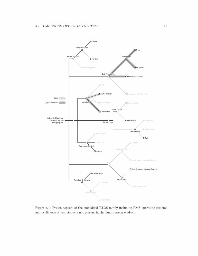
3.1. EMBEDDED OPERATING SYSTEMS 41
RMS
Cyclic Executive
Statistical
Declarative
Absent
Admission Controlon
Hardware
Task
HierarchicalMechanismnis
Impermeable
Permeable
Permeabilityabil
Partitioning
Static Priority
Rate-Based
EDF
Distributed
Schedulingulinggng
Mutexes
Synchronous Message Passing
Divisible Taske Ta
Asynchronous Message Passing
Linked Fragments
Atomic Taskc Ta
IPC
Embedded RealtimeOperating System
Design Space
Event-triggered
Externalizationzat
Global
Per-task
Time-triggeredgge
Preemptive Threads
Non-preemptive Threads
Task Abstractionstractiorac
Fixed
Adaptive
Performersormersme
Hard Realtime
Deadline SensitivityensenExtension
Incomplete
Soft Realtimealt
Figure 3.1: Design aspects of the embedded RTOS family including RMS operating systemsand cyclic executives. Aspects not present in the family are grayed-out.
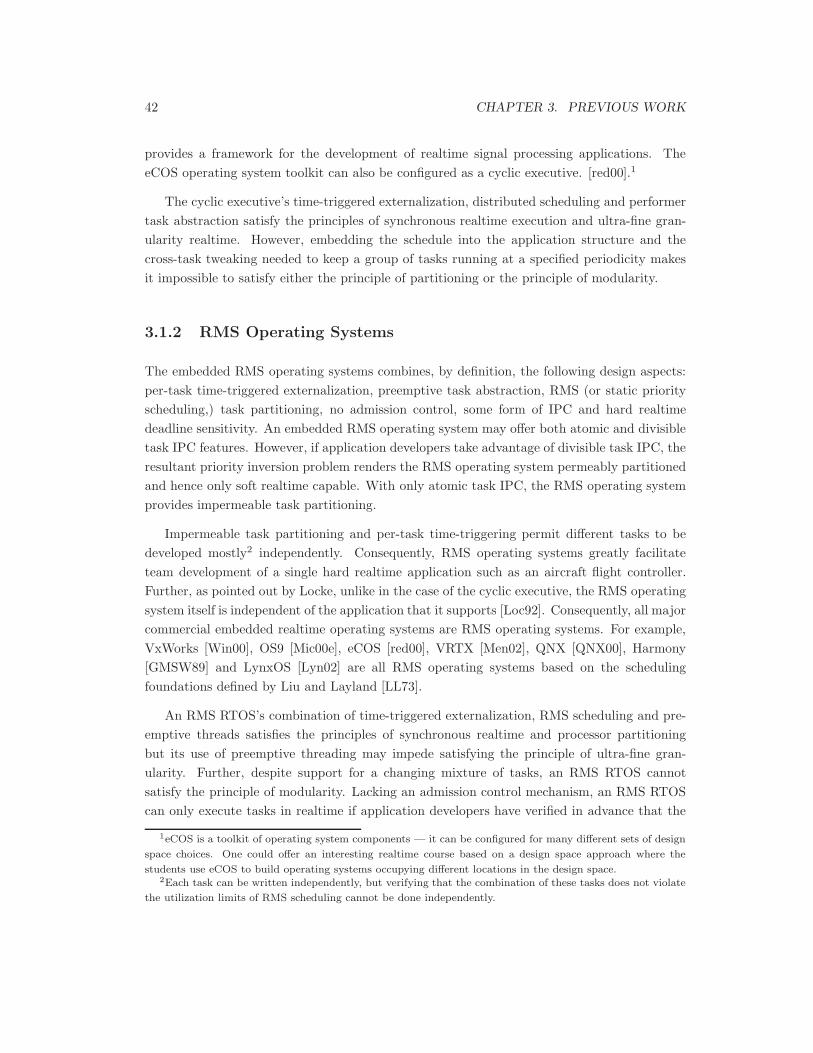
42 CHAPTER 3. PREVIOUS WORK
provides a framework for the development of realtime signal processing applications. TheeCOS operating system toolkit can also be configured as a cyclic executive. [red00].1
The cyclic executive’s time-triggered externalization, distributed scheduling and performertask abstraction satisfy the principles of synchronous realtime execution and ultra-fine gran-ularity realtime. However, embedding the schedule into the application structure and thecross-task tweaking needed to keep a group of tasks running at a specified periodicity makesit impossible to satisfy either the principle of partitioning or the principle of modularity.
3.1.2 RMS Operating Systems
The embedded RMS operating systems combines, by definition, the following design aspects:per-task time-triggered externalization, preemptive task abstraction, RMS (or static priorityscheduling,) task partitioning, no admission control, some form of IPC and hard realtimedeadline sensitivity. An embedded RMS operating system may offer both atomic and divisibletask IPC features. However, if application developers take advantage of divisible task IPC, theresultant priority inversion problem renders the RMS operating system permeably partitionedand hence only soft realtime capable. With only atomic task IPC, the RMS operating systemprovides impermeable task partitioning.
Impermeable task partitioning and per-task time-triggering permit different tasks to bedeveloped mostly2 independently. Consequently, RMS operating systems greatly facilitateteam development of a single hard realtime application such as an aircraft flight controller.Further, as pointed out by Locke, unlike in the case of the cyclic executive, the RMS operatingsystem itself is independent of the application that it supports [Loc92]. Consequently, all majorcommercial embedded realtime operating systems are RMS operating systems. For example,VxWorks [Win00], OS9 [Mic00e], eCOS [red00], VRTX [Men02], QNX [QNX00], Harmony[GMSW89] and LynxOS [Lyn02] are all RMS operating systems based on the schedulingfoundations defined by Liu and Layland [LL73].
An RMS RTOS’s combination of time-triggered externalization, RMS scheduling and pre-emptive threads satisfies the principles of synchronous realtime and processor partitioningbut its use of preemptive threading may impede satisfying the principle of ultra-fine gran-ularity. Further, despite support for a changing mixture of tasks, an RMS RTOS cannotsatisfy the principle of modularity. Lacking an admission control mechanism, an RMS RTOScan only execute tasks in realtime if application developers have verified in advance that the
1eCOS is a toolkit of operating system components — it can be configured for many different sets of design
space choices. One could offer an interesting realtime course based on a design space approach where the
students use eCOS to build operating systems occupying different locations in the design space.2Each task can be written independently, but verifying that the combination of these tasks does not violate
the utilization limits of RMS scheduling cannot be done independently.
3.2. HARDWARE PARTITIONING OPERATING SYSTEMS 43
processor usage of all possible combinations of tasks satisfy the constraints discussed in Sec-tion 2.5.2. That this verification must test all possible schedulable tasks excludes executingindependently-authored tasks and so cannot satisfy the principle of modularity.
Both the cyclic executive and the embedded RMS RTOS fail to satisfy the principle ofmodularity. Given that embedded applications do not execute independently-authored code,this failure does not reduce their utility. However, it does show that embedded operatingsystems cannot serve as multimedia operating systems.
3.2 Hardware Partitioning Operating Systems
Some embedded systems must implement tasks with contradictory scheduling requirementssuch as both time-shared and hard realtime tasks. Many computer systems provide such acapability with hardware partitioning — a separate physical processor for each schedulingdomain.
Examples of complete systems that use hardware partitioning include Motorola’s Streamer’s[Mot00], cellular phones based on Motorola’s DSP56651 [Mot98], Qualcomm’s BREW [Qua01],cellular phones based on its multi-core CDMA chipsets and PC-hosted digital television sys-tems based on the TeraLogic TL880 chipset [Mot00, Ter01]. Many other examples existas this is the most commonly used solution for commercial systems that need to executeboth hard realtime and soft or non-realtime tasks. The popularity of the hardware parti-tioning approach is sufficiently popular to have attracted significant tool development efforts[Wol94, QHG99, Axe, San03]. These systems use hardware partitioning to ensure that softrealtime execution cannot interfere with hard realtime execution.
Systems of this type have at least one processor that runs either an RMS or cyclic executivestyle embedded RTOS. However these systems have one or more additional processors thatexecute a different operating system. The design aspects of the complete system are the unionof the design aspects of the operating systems running on each of the different processors. Forexample, all of [Mot00, Qua01, Ter01] have two processors: a DSP-style processor runninga hard realtime cyclic executive and a more traditional processor running a general purposeoperating system. In these examples, the second operating system (OS-9, BREW and Win-dows respectively) provides soft or non-realtime execution [Mic00e, Qua01, Mic04]. The twoprocessors communicate via dedicated hardware such as a dual-ported memory or a pair ofFIFOs.
Hardware partitioning provides a completely impermeable partition between tasks on differ-ent processors. Consequently, developers can implement each processor’s tasks independentlybut at the cost of more complex hardware.3
3At least in the context of hardware such as set-top boxes or cellular phones, I suspect that an engineer-
44 CHAPTER 3. PREVIOUS WORK
The examples of hardware partitioning discussed above have two sources of inflexibility.First, they fix the resource allocation between physical processors at the time of designing thehardware. Second, they all use a fixed-function hard realtime cyclic executive on the realtime-dedicated processor. The first inflexibility is an intrinsic property of hardware partitioning andcan only be remedied with one of the software partitioning schemes discussed below. Driven bya need for versatility, many realtime systems require the ability to execute a changing mix ofhard realtime signal processing applications on the realtime-specific processor. The remainderof this section discusses a solution: an extensible cyclic executive.
An extensible cyclic executives augments a cyclic executive with a functional scheduler andan admission control mechanism. A fixed-function cyclic executive is merely a set of re-usablelibraries that an application developer statically links into the application and is just barelyan OS. However, an extensible cyclic executive is a true, albeit small, OS — it manages theresource needs of multiple dynamically chosen tasks. With the inclusion of admission control,an extensible cyclic executive has the following design choices: time-triggered externalization,performer task abstraction, distributed scheduling, hardware partitioning between it and thehost processor and permeable task partitioning internally, atomic task IPC and declarativeadmission control. Figure 3.2 shows the design aspects of such an operating system.
The DSP-like devices known as “media processors” such as the HRV [NK91, HBJS91],Mwave [Tex92] and Trimedia processors [Sla97] are relevant examples because their combi-nation of hardware partitioning and an extensible cyclic executive has the same purpose asLiquiMedia: a system optimized for the generation of information streams. Of these, theMwave is described in more detail below because [Tex92] contained the most complete archi-tectural description.4
The MWave was designed to be attached to a PC as an intelligent co-processor for time-varying media. Its system software consisted of two components: an admission control frame-work and scheduling package running on the PC host and a cyclic executive running on theMwave’s DSP.
The PC-hosted scheduler packed performers into one of three round-robin scheduling tablesbased on a task’s declared performance statistics and desired execution rate. The scheduleraccepts additional tasks for the Mwave so long as sufficient unallocated time in the scheduleremains to hold the new task. Tasks must declare a worse-case upper bound on their processorneeds.
A hardware interval timer provided time-triggered externalization at a different rate foreach of the scheduling tables. The dispatch frequency of the different schedules reflected the
ing organization’s most economical choice in this trade-off depends primarily on the proportion of electrical
engineers and computer scientists in the organization. Members of each discipline will prefer the additional
complexity in the domain that they find most comfortable.4In some ways, the Chromatic media accelerator makes a better example but as the company (and conse-
quently the white papers on its web site) has ceased to exist, I cannot provide a citation for its features.
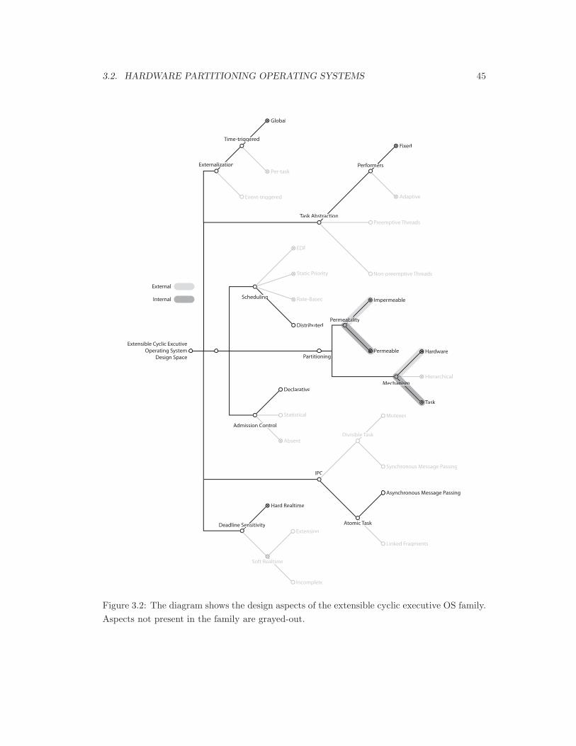
3.2. HARDWARE PARTITIONING OPERATING SYSTEMS 45
External
Internal
Statistical
Declarative
Absent
Admission Controlon
Hardware
TaskT
HierarchicalMechanismanismnis
Impermeable
Permeable
Permeabilityeabilityaabil
Partitioning
Static Priority
Rate-Based
EDF
Distributed
Schedulingngng
Mutexes
Synchronous Message Passing
Divisible Taske Ta
Asynchronous Message Passing
Linked Fragments
Atomic Taskc Ta
IPC
Extensible Cyclic ExcutiveOperating System
Design Space
Event-triggered
Externalizationzat
Global
Per-task
Time-triggeredgge
Preemptive Threads
Non-preemptive Threads
Task Abstractionrac
Fixed
Adaptive
Performersme
Hard Realtime
Deadline SensitivityensenExtension
Incomplete
Soft Realtimealt
Figure 3.2: The diagram shows the design aspects of the extensible cyclic executive OS family.Aspects not present in the family are grayed-out.

46 CHAPTER 3. PREVIOUS WORK
intended applications of the processor: joystick and MIDI support, software modem emulationand music synthesis. Tasks dispatched at higher frequency interrupt tasks dispatched at lowerfrequencies. As a result, some of the tasks on the Mwave do not execute atomically. Neverthe-less, these are performer-style tasks because the Mwave’s operating system never interleavesthe execution of tasks at a single dispatch rate.
The Mwave provided asynchronous message passing IPC via dual-ported hardware ringbuffers. These permitted communication between tasks on the Mwave itself and betweenthe host processor and the Mwave. In summary, the Mwave has an extensible cyclic executiveoperating system with the following design choices: global time-triggered externalization, fixedperformer task abstraction, distributed scheduling, task partitioning and atomic task IPC.
Sun’s High Resolution Video workstation (HRV), combined a workstation with a pro-grammable video processing board built out of multiple i860 processors. The HRV was thesuccessor to Sun’s TAAC-1 board, that though not marketed as such, is another exampleof a hardware-partitioned media processor. The video board executed a custom RTOS op-timized for media processing. The HRV communicated both internally and with its non-realtime SunOS host via asynchronous message passing over a conduit. Conduits includeda rate-balancing abstraction that permitted realtime and non-realtime processing to remainsynchronized [NK91].
SGI’s REACT realtime extension to IRIX provides another example of a hardware parti-tioned extensible cyclic executive. As discussed below in Section 3.4, REACT provides dis-tributed scheduling of hard realtime performers. To insure realtime operation even while shar-ing system resources with IRIX, one or more physical processors must be exclusively dedicatedto realtime REACT tasks [CT00].
Hardware partitioning systems such as HRV and Mwave were purpose-built to providemultimedia operating system functionality and so satisfy the principles of partitioning, syn-chronous realtime and ultra-fine granularity realtime. However, these systems only permitprivileged applications to submit and execute tasks on the dedicated realtime hardware. Con-sequently, they do not support the execution of arbitrary independently-authored realtime anddo not satisfy the principle of modularity.
3.3 Media Generation Frameworks
Multimedia stream generation, particularly the playing of digitally compressed music andvideo, is by far the most common realtime application on general purpose operating systems.5
Consequently, there are a number of media generation frameworks that attempt to provide
5It’s the only one actually shipped with all major general purpose operating systems.
3.3. MEDIA GENERATION FRAMEWORKS 47
a virtual signal-processing co-processor for the generation of multimedia streams. Each me-dia generation framework (MGF) has the same function and the same design aspects as theRTOS running on a hardware media processor such as the Mwave. A MGF has time-triggeredexternalization, the performer task abstraction, permeable task partitioning, declarative (orabsent) admission control, distributed scheduling and atomic task IPC.
Apple’s QuickTime, Microsoft’s DirectShow and the Java Media Framework are the bestknown commercial MGF examples [App00b, Mic00a, Mic04, Jav00].6 A sizable number of otherframeworks exist including GnomeMedia, MET++, and GStreamer [Lee01, Tay01, AEW01].QuickTime is the seminal example of a MGF and has inspired the architecture of the others.7
Consequently, the following focuses on QuickTime.
In all of these examples, the realtime behaviour of the MGF is at the mercy of the underlyinggeneral purpose operating system. The Java Media Framework (JMF), is at the mercy oftwo: the “operating system” of the Java virtual machine and whatever operating system liesunderneath it. Clearly the MGF operates best as a client RTOS of a parent OS that hasthe impermeable hierarchical partitioning design aspect. Windows 2000 attempts to providea form of hierarchical partitioning for its native MGFs and this is discussed further below.
QuickTime is a multifaceted product. It contains a partitioning framework, an admissioncontrol mechanism, a scheduler, an IPC mechanism optimized for communications betweentasks performing media processing and a container-based file-format [Hod94, Wan95, App00b].The QuickTime container format or “movie” provides an arbitrary hierarchy of “media” objectsthat can correspond to the hierarchy of substreams comprising an information stream. Eachmedia object references some underlying block of data, either on local storage, or, in a recentdevelopment, as RTP streaming content. For example, a movie is a track of sound and a trackof images, where the sound may itself be comprised of multiple separate instruments and theimages may consist of some arbitrary combination of text, sprites, realtime animation andcompressed image sequences. QuickTime’s media model is sufficiently general to encompassthe entire display capabilities of modern computers as compared to the fixed capabilities ofthe MPEG-1 format [Tek95].
An application that wishes to use the QuickTime framework must begin by building adata flow graph of components. Once QuickTime begins processing media data, it repeatedlyinvokes the components at their desired invocation rates and executes them atomically eachtime. Components provide a performer-style task abstraction.
QuickTime does not provide an admission control framework for its components. Instead,QuickTime components are adaptive-style performers. A correctly written QuickTime com-ponent must adapt its processing internally to keep its execution time below the upper bound
6Microsoft continues to radically alter DirectShow with each release. Consequently, it is difficult to accu-
rately determine its current abilities.7Apple filed suit against Microsoft on the grounds that DirectShow borrowed too much of its architecture
from QuickTime [App95].
48 CHAPTER 3. PREVIOUS WORK
permitted by the schedule. QuickTime defines interfaces by which the framework informsa component of the currently acceptable maximum running time. For example, consider aQuickTime video decompression component. On a fast machine, the component generates afull frame thirty times per second. On a slower machine, the video playback remains synchro-nized to the audio track but each invocation of the component generates only 1/6 of a frame —resulting in a frame-rate of only five frames per second. A human audience’s sensory modal-ities impose different timeliness requirements on the various tasks comprising a multimediaapplication. The QuickTime framework integrates an importance mechanism that attemptsto respect them.
The data flow graph provides inter-component IPC. Components operate on buffers ofmedia information. Components invoke QuickTime functions to retrieve data buffers fromupstream components and to write processed buffers to downstream components. QuickTimeincludes several functions for buffer management. Sample buffers are equivalent to messagesand so constitute an instance of asynchronous message passing.
At the time of constructing the dataflow graph, the application must also specify a timebasefor each component. The QuickTime framework dispatches each component at the specifiedrate. At the time of instantiation, QuickTime prepares a table that schedules componentexecution.8
QuickTime permits every component to have a separate time base. QuickTime containsan embedded time base component that takes care of obtaining the actual external timefrom a hardware clock and scaling and shifting this as required for each component. Oneof QuickTime’s foremost strengths as a framework for the generation of multimedia streamsis its ability to generate them synchronized to external time. Clearly, this is per-applicationtime-triggered externalization.
QuickTime components execute in a permeable hierarchical partition as each applicationis responsible for making function calls into QuickTime to give the framework time to executemedia processing components. Requiring cooperative applications is QuickTime’s most signif-icant weakness as a framework for signal processing — not only is there no enforced explicitallocation of resources to the media processing components, but the scheduling of what shouldbe realtime components is not even exposed to the operating system. For example, an appli-cation may inadvertently starve its own realtime components by lingering in its non-realtimecode.
Originally, Apple developed QuickTime for a a non-preemptively scheduled version of Ma-cOS [App88]. Consequently, a correct application could guarantee realtime operation of its ownQuickTime components by never letting other applications run. MacOS X has eliminated this“feature” by being based on the Mach microkernel. Despite Mach’s inclusion of static priority
8The documentation does not exactly specify how QuickTime creates its schedule. I believe that this is
deliberate.

3.3. MEDIA GENERATION FRAMEWORKS 49
scheduling, the version of Mach found in MacOS X is not an RTOS [App97, Raj00]. Quick-Time’s poor performance on MacOS X demonstrates the importance of running a MGF insidean impermeable partition on an RTOS [App00a]. However, experience with MacOS X 10.3suggests that Apple has significantly improved QuickTime’s realtime performance. Core Im-age coupled with programmable GPUs will add hardware partitioning to QuickTime [App04].QuickTime also executes on Microsoft WindowsNT where it continues to exhibit performanceproblems caused by its lack of partitioning.
Microsoft’s DirectShow provides similar functionality to QuickTime. The ASF and AVI fileformats correspond to the QuickTime container file format. DirectShow permits applicationsto build “filter graphs”. The filter is an adaptive-style performer equivalent to the QuickTimecomponent. The DirectShow library contains a wide assortment of pre-defined filters. The filtergraph provides a framework for asynchronous message passing IPC between the filter instancescomprising any one graph. Applications may provide their own filters. In DirectShow, thefilter graph also distributes a single clock to all the filters thereby providing DirectShow filterswith global time-triggered externalization.9 Filters drive adaptation by distributing qualitymessages which instruct upstream filters to either reduce or increase the quantity of dataproduced.
Unlike QuickTime, DirectShow attempts to provide a more impermeable partitioning be-tween filters and non-realtime applications. When running on Windows 2000, selected filtersare actually stubs that control filters executing in the context of the operating system kernel.These kernel streaming drivers execute at a priority that protects them from preemption bynon-realtime applications [Sol98]. However, kernel streaming filters are not truly realtime asthe kernel’s processing of I/O requests can still preempt them in un-predictable ways [DN99].10
Non-privileged applications cannot install a kernel streaming driver.11
The Java Media Framework (JMF) also provides a synchronous framework similar to Quick-Time or DirectShow [Jav00]. An application uses the JMF just as a QuickTime applicationuses the QuickTime API.12 An application first instantiates fixed performer-style media pro-cessing components and connects them together into a filter graph. The filter graph providesa framework for asynchronous message passing IPC. A clock base component provides thevarious JMF components with per-application time-triggered externalization. Through theJava language’s support for interfaces, the JMF makes it possible to easily add new media
9Two different Windows applications could have different clocks if they succeeded in using DirectShow
simultaneously. In practice, I have observed that each DirectShow filter tends to take exclusive ownership of
any associated hardware resources.10The existence of Rialto (discussed below in section 3.6.2) suggests that Microsoft will eventually attempt
to correct this limitation.11Information on the development of kernel streaming drivers is difficult to obtain.12Apple’s QuickTime development staff seemed quite contemptuous of the JMF — describing it as an in-
complete copy [Nar99]. I agree with this assessment: JMF is, for all practical purposes, a functional subset of
QuickTime. However, on the Win32 platform, JMF is easier to develop with.

50 CHAPTER 3. PREVIOUS WORK
processing components.
Like QuickTime, the JMF provides no admission control. Unlike QuickTime or DirectShow,the JMF framework does not specify a running time to its performers so they could consumeall available processor resource. Fortunately, JMF does partition its performers from othercode by invoking them as dedicated threads. This partition is, however, extremely permeableas Java threads lack processor reservation and exhibit considerable scheduling variance causedby garbage collection and an imprecise scheduling model.13
Of existing research partitioning frameworks, GStreamer appears to be the most complete[Tay01, LT96, FM01]. The designers of GStreamer copied most of its architecture from Direct-Show. Most of the changes were practical improvements. GStreamer has fixed performer-styletasks, a connected graph of components, a reasonably rich library of components and fullysupports execution of user-provided components. The IPC mechanism continues to be asyn-chronous message passing between atomic tasks, but appears from inspection to be much moreefficient.14
All four MGFs discussed above were designed for multimedia stream generation, partic-ularly digital music and video playback. Each framework has time-triggered externalization,the performer task abstraction possibly with adaptive execution time specification, perme-able hierarchical partitioning externally and permeable task partitioning internally, little orno admission control, distributed scheduling and asynchronous message passing IPC. Theseframeworks all attempt to provide a software emulation of the combination of a DSP and ageneral purpose processor (c.f. 3.2) by embedding a DSP-like execution environment inside ageneral purpose operating system. However, all of the discussed frameworks fail to satisfy anyof the principles of a multimedia operating system because none of the MGFs actually executein realtime and all four principles require realtime execution of stream-generating code.
3.4 Distributed Scheduling Operating Systems
A wide variety of general purpose realtime operating systems exist. I categorized these RTOSsinto families by their scheduling and partitioning mechanisms. Distributed scheduling oper-ating systems combine time-triggered externalization, performer-style tasks, (permeable) taskpartitioning, distributed scheduling and declarative admission control. With only declara-tive admission control, this RTOS family fails to satisfy the principle of modularity. Relevantexamples include Spring because it uses distributed scheduling in a manner similar to LiquiMe-
13See Appendix D for additional information on the JMF and how some of its limitations can be rectified.14Application-provided filters must link against DirectShow COM objects to have access to media data.
Component developers for GStreamer compile media data access macros into their components as GStreamer
is available as source.

3.4. DISTRIBUTED SCHEDULING OPERATING SYSTEMS 51
dia [SR91] and MediaVMS [VRT96] and REACT [CT00, VRT96] because both have realtimecapabilities intended for information stream generating applications.
Spring15 is a hard realtime RTOS with per-task time-triggered externalization, performertasks, distributed scheduling and declarative admission control. Given each task’s desireddispatch rate and its WCET, the Spring “planning scheduler” verifies that it can successfullyinterleave the execution of the tasks and, if so, constructs a fully enumerated schedulingfunction. Spring has distributed scheduling because the scheduling function is constructed byan external agent — albeit one provided by the operating system.
Spring is a distributed RTOS as the operating system manages resource allocations on anetwork of homogeneous processors. Spring uses both hierarchical and hardware partition-ing to separate different classes of tasks. In particular, Spring supports event-triggered tasksby executing them inside a partition created from a time-triggered task. The Spring kernelschedules I/O and memory resources in addition to processor resources. Processor nodes com-municate via asynchronous message passing [SR91]. With only declarative admission control,Spring can only support independently authored tasks by isolating them on physically separateprocessor nodes. Consequently, it fails to support the principle of modularity.
Digital Equipment Corporation produced an interesting operating system that uses imper-meable hierarchical partitioning to provide three distinct sub-operating systems with differingdeadline sensitivities, task abstractions and schedulers [VRT96]. In the absence of a name,I dubbed this RTOS “MediaVMS”.16 MediaVMS’s hard realtime partition has distributedscheduling, declarative admission control and the performer task abstraction. A planningscheduler similar to Spring’s constructs the fully-enumerated scheduling function if the admis-sion control mechanism verifies that the OS can successfully interleave the execution of tasksat their desired invocation rates. As with Spring, MediaVMS relies on declared performerrunning times and so fails to satisfy the principle of modularity.
SGI’s REACT realtime extension to IRIX also uses a distributed scheduler for realtimeperformer-style tasks [CT00]. REACT uses distributed scheduling for maximum versatility:applications may implement any desired scheduling policy on top of REACT.17 However,REACT has no admission control mechanism. Consequently, only privileged applications mayexecute in realtime and so REACT fails to satisfy the principle of modularity.
With the combination of hierarchical partitioning, distributed scheduling, time-triggeredexternalization and the performer task abstraction, these systems satisfy the principles of pro-cessor partitioning, synchronous realtime and ultra-fine granularity realtime. However, all ofthese systems have only declarative admission control and so cannot schedule tasks successfully
15Note that this Spring operating system is completely unrelated to Sun’s distributed non-realtime Spring
kernel [MGH+95].16The literature did not specify if VMS code was involved but it seems a fitting name.17See [KSSR96] for an example.
52 CHAPTER 3. PREVIOUS WORK
unless applications provide correct WCETs. An OS cannot rely on an independently-authoredapplication to do so and so none of these systems can satisfy the principle of modularity.
3.5 Hierarchical Partitioning Operating Systems
Section 3.2 discusses RTOSs that use separate physical processors to guarantee resource al-locations to different classes of tasks. Hardware partitioning is inflexible and requires multi-processor hardware. Hierarchical partitioning provides one possible alternative: the operatingsystem executes different classes of tasks on impermeably partitioned virtual processors.
A hierarchically partitioned operating system is really two or more operating systems inone: a simple realtime “parent” operating system and one or more “child” operating systemsnested inside the parent operating system’s tasks. Parent operating systems are (sometimessimplified) RMS RTOSs. Implementers choose child operating systems suitable to the appli-cation domain.
Many systems use hierarchical partitioning on an RMS parent OS to provide multiplescheduling domains. For example, [KSSR96, AB99, AB98a, GGV96, AB98b, TH97, JLS99,CS01, SCG+00] all present RMS RTOSs enhanced with one or more tasks containing somekind of child operating system. In each case, the parent RMS RTOS provides hard real-time capabilities while children RTOSs executing soft realtime tasks provide improved systemutilization and versatility over a pure RMS RTOS.
Yodaiken’s RTLinux and Digital’s MediaVMS also use hierarchical partitioning to combinetasks with radically different scheduling domains in a single operating system. These two sys-tems are similar to LiquiMedia in their use of hierarchical partitioning and warrant additionaldiscussion.
RTLinux adds hard realtime capability to Linux by virtualizing the hardware’s interruptcontrollers and running an essentially unchanged Linux kernel on top of a small hard realtimeexecutive [Yod96, Bar97, www00b]. The RTLinux executive layer traps all incoming interruptsand dispatches them to one of its two tasks. The higher priority parent task executes performer-style tasks in response to the incoming interrupts. The second task virtualizes the PC hardwareto run a nearly unmodified Linux kernel as its child operating system. RTLinux’s use ofhierarchical partitioning enabled Barabanov to easily add realtime capabilities to Linux.
To prevent priority inheritance and leave the Linux kernel non-reentrant, the RTLinuxexecutive and non-realtime Linux applications communicate via non-blocking FIFOs that im-plement asynchronous message passing IPC.
RTLinux realtime tasks run in kernel context and can easily damage the system. RTLinuxdoes not provide an admission control mechanism. Consequently, without either memory

3.6. TASK PARTITIONING OPERATING SYSTEMS 53
access or processor use protection, RTLinux permits only privileged users to install realtimetasks and so does not satisfy the principle of modularity.
As later advocated by Pawan et al. [PJG+01], Digital’s MediaVMS uses an RMS parentoperating system to provide an impermeable partition between three child operating systems[VRT96]. Each child operating system provides distinct scheduling and task design aspects:hard realtime performers with distributed scheduling, soft realtime non-preemptive threadswith distributed (round-robbin) scheduling and non-realtime time-shared preemptive threads.Oddly, despite including every task abstraction, MediaVMS omits an IPC mechanism betweentasks in the different child operating systems. While this insures an impermeable partition,it also prevents application developers from appropriately dividing their applications acrossMediaVMS’s versatile combination of scheduling and task abstractions.
As with Spring and REACT, MediaVMS and RTLinux satisfy the the principles of pro-cessor partitioning, synchronous realtime and ultra-fine granularity realtime. However, all ofthese systems provide only declarative admission control and so fail to satisfy the principle ofmodularity.
3.6 Task Partitioning Operating Systems
The previous section discussed operating systems that use hierarchical partitioning to providea range of specialized task abstractions and scheduling mechanisms. Many operating systemsdemonstrate a contrasting design choice: a single task abstraction and scheduling mechanismthat attempts to handle all application needs ranging from month-long batch jobs to millisec-ond response control systems.
Task partitioned operating systems have preemptive threading, rate-based scheduling, per-meable task partitioning, divisible task IPC, declarative admission control and soft realtimedeadline sensitivity. Figure 3.3 summarizes the location of task partitioning operating systemsin the design space.
Given that the task partitioning operating system is a full-blown self-hosted operatingsystem, it represents a popular development project. Relevant examples include the seminalwork on Realtime Mach [Raj91]; and Rialto [JIF+96], YARTOS [JB95], DiRT [SAWJ+96],SMART [Nie99] and Scout [BPM99] because the primary intended use of their realtime facilitiesis the implementation of multimedia applications. Each of these operating systems is discussedin turn below. Other similar examples include ARC-H [Yau99], which combines rate-basedscheduling with hierarchical partitioning, and BEST [BB02], which improves Linux’s ability toschedule soft realtime tasks by automatically placing them in a rate-based realtime schedulingclass.

54 CHAPTER 3. PREVIOUS WORK
Statistical
Declarative
Absent
Admission Controlon
Hardware
Task
HierarchicalMechanismnis
Impermeable
Permeable
Permeabilityabil
Partitioning
Static Priority
Rate-Based
EDF
Distributed
Schedulingngng
Mutexes
Synchronous Message Passing
Divisible Taske Ta
Asynchronous Message Passing
Linked Fragments
Atomic Taskc Ta
IPC
Task PartitioningOperating System
Design Space
Event-triggered
Externalizationzat
Global
Per-task
Time-triggeredgge
Preemptive Threads
Non-preemptive Threads
Task Abstractionrac
Fixed
Adaptive
Performersme
Hard Realtime
Deadline SensitivityensenExtension
Incomplete
Soft Realtimealt
Figure 3.3: Design aspects shared by the task partitioning OS family. Aspects not present inthe family are grayed-out.

3.6. TASK PARTITIONING OPERATING SYSTEMS 55
3.6.1 Realtime Mach and Descendants
Realtime Mach (RTMach) is one of the earliest task partitioned operating systems. Rajkumarcreated RTMach by adding a priority inheritance mechanism to the basic Mach kernel [Raj91].Mach is a non-realtime microkernel built around three principal features: preemptive threads,synchronous message passing and flexible memory management [RJO+89]. With the additionof priority inheritance, RTMach supports soft realtime execution with static priority or EDFscheduling, permeable task partitioning and declarative admission control.
In search of superior realtime stream-generation performance, Mercer and Rajkumar ex-tended Realtime Mach with a mechanism called processor capacity reserves [MST93, MST94].A capacity reserve is a reservation of processor time based on a percentage of the processor anda periodicity. An application running under Realtime Mach with capacity reserves (RTMcr)specifies the percentage of processor that it requires and the periodicity of its needs. Conse-quently, RTMcr augments Realtime Mach with time-triggered externalization, and declarativelifetime admission control.
Mach’s micro-kernel architecture significantly complicates RTMcr’s implementation of taskpartitioning. Capacity reserves must allocate fixed proportions of the processor resourcesper application rather than per task. In a micro-kernel, an application task interacts withsystem services such as a file system by sending a synchronous message to the service task.Consequently, an application using only a single task may cause a significant number of othertasks to consume processor resources. Consequently, RTMcr must correctly “bill” the processoruse of system service tasks back to the application tasks which were responsible for invokingthem. Tracking these dependencies complicates RTMcr’s implementation of task partitioningand increases the implementation overhead of a synchronous IPC operation.
RTMcr provides a choice of either EDF scheduling or static priority scheduling. Thestatic priority scheduler provides a firm task partition but at the cost of reduced utilization.Conversely, RTMcr’s EDF scheduler provides higher utilization levels but cannot prevent ahabitually overtime application from starving even higher priority applications.
In subsequent research, Rajkumar et al. have added capacity reserves to both Linux [OR98]and Java [dNR00]. The introduction of hierarchical capacity reserves in [MR01] resolves thedifficulty of “billing” resource use to specific applications in uncooperative environments andhelps satisfy the principle of modularity. However, complexity of usage tracking in thesesystems precludes satisfying the principle of ultra-fine granularity.
The combination of capacity reserves, preemptive tasks and static priority scheduling satisfythe principles of partitioning and synchronous execution and at least partially satisfy theprinciple of modularity. However, the cost of tracking an application’s execution time acrossmultiple service threads prevents RTMcr and its descendants from satisfying the principle ofultra-fine granularity.
56 CHAPTER 3. PREVIOUS WORK
3.6.2 Rialto
Jones et al. designed Rialto to support the execution of independently authored realtimeand non-realtime fragments. They intended Rialto to support both traditional time-sharedprocessing tasks and tasks for realtime stream generation [JIF+96, JLDI95, Jon93]. Rialtocombines preemptive threads, almost impermeable task partitioning, fluid-flow style rate basedscheduling, instantaneous and lifetime declarative admission control, divisible task IPC andsoft realtime deadline sensitivity.
Rialto’s resource planner provides lifetime admission control. An application actually ob-tains a guaranteed task partition by negotiating with the resource planner. Rialto improvessystem usability by letting users control inter-application resource negotiation.
Rialto uses fluid-flow scheduling. The scheduler runs threads in order of descending laxity.Laxity is a metric ordering threads by deadline and size of constraint block. A constraint blockis a portion of a thread with realtime constraints and will be discussed further below. Laxityis similar to the lag metric found in DiRT’s Earliest Eligible Virtual Deadline First (EEVDF)scheduling. Threads with the smallest estimated constraint block and earliest deadline executefirst.
In Rialto, developers specify an application’s realtime constraints with a novel mechanism:the constraint block. Unlike tasks in other task partitioning RTOSs, Rialto tasks are not re-altime by default — only their constraint blocks execute in realtime. Developers specify therealtime portions of a task by wrapping them with BeginConstraint() and EndConstraint()
functions. The arguments of BeginConstraint() specify the realtime constraints of the en-closed code: its release time, deadline, estimated running time and importance.
Rialto uses these parameters to provide declarative instantaneous admission control: Be-
ginConstraint() returns true if the processor can successfully execute all live constraintblocks before their deadlines and after their start times.18 An application specifies the relativeimportance of its constraint blocks with the importance argument. The scheduler sacrificesthe execution of less important constraint blocks in a transient overload situation.
When combined with task partitioning, constraint blocks partially satisfy the principle ofpartitioning. They permit developers to partition the expression of realtime and non-realtimecode. However, Rialto cannot consistently enforce this partition because it can only partitionrealtime and non-realtime code along task boundaries and a single task can contain both typesof code.
Every new constraint block encountered can change the task’s laxity and result in a contextswitch. Consequently, Rialto imposes a minimum 10ms quantum on task preemptions to im-prove system efficiency by reducing the number of context switches. The large 10ms quantumfails to satisfy the principle of ultra-fine granularity realtime.
18The start time is optional. If no start time is provided, the current time serves as the default.

3.6. TASK PARTITIONING OPERATING SYSTEMS 57
Rialto provides mutex style IPC. To prevent the consequent vulnerability to priority inver-sions, it provides constraint inheritance. Constraint inheritance generalizes priority inheritanceto constraint blocks: blocks in lower laxity tasks inherit the deadlines of blocks in higher laxitytasks that are blocked on them. Constraint inheritance increases the variability of constraintblock running time so allows Rialto to provide only soft realtime scheduling.
While only having declarative admission control, Rialto’s combination of RBE schedulingand preemptive threads satisfy the principle of modularity. Further, constraint blocks ad-equately satisfy the principles of partitioning and synchronous realtime. However, Rialto’s10ms thread quantum fails to satisfy the principle of ultra-fine granularity’s realtime.
3.6.3 YARTOS and DiRT
Jeffay and Bennett’s YARTOS was one of the first task-partitioned operating systems thatused rate-based scheduling [JB95]. It has RBE scheduling, preemptive threads, almost imper-meable task partitioning, divisible task IPC, declarative admission control and soft realtimedeadline sensitivity. YARTOS showed that rate-based scheduling could successfully providetask partitioning and soft realtime task execution.
Subsequently, Stoica et al. extended Realtime Mach with a fluid-flow rate-based schedulercalled “proportional share” to implement DiRT [SAWJ+96]. Proportional share schedulingprovides a reasonably impermeable task partition based on task importance and a declarativeadmission control mechanism. DiRT’s proportional share scheduling requires time-triggeredexternalization.
Stoica et al. showed that the DiRT scheduler provides provably correct processor partition-ing with an execution latency not more than the smallest possible task period d′p,i. Further-more, DiRT’s EEVDF intrinsically handles priority inversion problems by being an extensionof EDF scheduling.19 Thus, the EEVDF scheduler provides impermeable task partitioning.As a result, DiRT does a good job of handling transient overtimes and even tasks that declareincorrect processor requirements.
However, DiRT’s EEVDF scheduling, like all rate-based schedulers, has two limitations.First, it cannot provide hard realtime guarantees. Second, EEVDF scheduling is complex andtime consuming: it requires O(log n) time to choose the next executable task from n tasks —a cost incurred at every context switch.
Despite only having declarative admission control, both YARTOS and DiRT satisfy theprinciple of modularity with a combination of RBE scheduling and preemptive threading.Their task-based partition also satisfies the principle of partitioning while time-triggered ex-ternalization and realtime execution satisfy the principle of synchronous realtime. However,
19Section 2.5.4 describes the EEVDF scheduling function.

58 CHAPTER 3. PREVIOUS WORK
YARTOS and DiRT cannot satisfy the principle of ultra-fine granularity realtime because theyboth have large context switch and scheduling overhead.
3.6.4 SMART
Nieh implemented SMART by extending Solaris with an RBE-style rate-based scheduler [NL97,Nie99]. Nieh extensively evaluated SMART using real-world loads and optimized SMART forreal-world job mixes. SMART demonstrated that, despite its complexity, an RBE schedulercan operate well in practice for a mixture of soft realtime, interactive and non-realtime tasks.However, SMART has relatively poor jitter and deadline accuracy. Consequently, SMARTcannot successfully execute hard realtime tasks.
SMART satisfies the principles of partitioning, synchronous realtime and modularity. How-ever, SMART uses Solaris threads and as will be shown in Section 6.4.2, Solaris threads arenot sufficiently efficient to support the principle of ultra-fine granularity.
3.6.5 BERT
Bavier et al. implemented a scheduler called “best effort realtime” (BERT) for the Scoutoperating system. BERT uses fluid-flow rate-based scheduling, augmented with an importancemechanism called “resource stealing”.
In BERT, instantaneous declarative admission control prevents transient overloads by hav-ing each slice declare its deadline and execution time size. Bavier et al. postulate a mechanismto track the trustworthiness of each task’s estimates of its per-slice running time as BERTcannot successfully maintain task partitions in the presence of chronic underestimates of aslice’s running time. If a slice over-estimates, other slices can resource steal from its unusedshare.
Scout also has an lifetime declarative admission control mechanism. The Scout admissioncontrol mechanism only accepts tasks if their declared resource and periodicity requirementscan be met on average.
3.6.6 Summary
All of the above operating systems occupy a similar location in the design space. They usepreemptive threading, rate-based scheduling, divisible task IPC, declarative admission controland nearly impermeable task partitioning. This common set of design space choices is mutuallydependent. Task partitioning requires preemptive tasks to successfully partition. Given a suc-cessful task partition, an admission control failure is not catastrophic so declarative admission

3.7. STATISTICAL ADMISSION CONTROL 59
control is sufficient. Finally, these operating systems favour time-triggered externalizationfor the same reason as the media generation frameworks: multimedia stream generation isthe dominant realtime application of a general purpose operating system and time-triggeredexternalization best addresses the synchronization needs of multimedia applications.
3.7 Statistical Admission Control
All the operating systems discussed above have either no admission control mechanism ordeclarative admission control. This section discusses operating systems in the two sub-aspectsof statistical admission: declared statistical admission control (DSAC) and empirical statisticaladmission control (ESAC).
3.7.1 DSAC OSs
All DSAC OSs: [AB99, AB98a, AB98b, TDS+95, ZHS99, MEP01, APLW02] use statisticaladmission control to increase processor utilization for soft realtime tasks. These systemshave soft realtime scheduling, preemptive threads, time-triggered externalization, typicallyhierarchical partitioning and declarative statistical admission control.
Tia et al. first presented the idea that relaxing WCET constraints on time-triggered taskslices improves processor utilization [TDS+95]. Instead of WCET bounds, they used a proba-bility distribution function known to correspond to the distribution of each slice’s tp,i,j . Theyshowed that probabilistic bounds provide significantly greater processor utilization.
Tia et al. describe two separate operating system architectures using statistical admissioncontrol. The first architecture uses hierarchical partitioning with a sporadic bandwidth serverexecuting thread-style tasks inside a single task of an RMS parent operating system. Thesecond architecture combines task partitioning, rate-based scheduling and statistical admissioncontrol. Here, Tia et al. extend an EDF scheduler with “slack stealing” to create a fluid-flow scheduler that uses computed estimates of a slice’s likely running time for instantaneousadmission control.
Atlas and Bestavros simulated a system called SRMS [AB98b]. SRMS extends a traditionalRMS preemptive RTOS with statistical admission control. An SRMS task p has a fixedperiodicity and a probability density function φp(t) for the processing time of a slice of p.SRMS defines QoS to be the minimum probability that over many releases, the overall taskmeets its relative deadline d′p:
QoS =∫ d′
p
0
φp(t)dt.
SRMS admits a set of tasks to the schedule if each task can receive an appropriate averageexecution allowance, in other words, if QoS exceeds an appropriate minimum value. The
60 CHAPTER 3. PREVIOUS WORK
underlying RMS scheduler provides a binary partition between higher priority hard realtimetasks and statistically-scheduled tasks.
SRMS has two potential limitations. First, the SRMS system requires a priori knowledgeof φp(t). Second, it can require the performance of statistical calculations in the critical pathof the scheduler.
Manolache et al.’s work is a natural extension of SRMS [MEP01]. It implements DSAC forevent-triggered tasks with arbitrary precedence relationships. However, it still requires eachtask to provide the PDF for its execution time.
Zhou et al. simulate another extension of RMS with a probabilistic task model [ZHS99].They use the task model of Atlas and Tia: time-triggered tasks with a known periodicity andindependent running time PDFs. They generalize Liu and Layland’s feasibility to tasks witha non-unity probability of meeting their deadlines.
When the running times of tasks are probabilistically bounded, the entire system’s feasi-bility,
feasibility =∏∀p
∫ d′p
0
φp(t)dt, (3.1)
is stochastic. Because RMS tasks have different periodicities, a straight-forward evaluationof equation 3.1 does not provide good results. Consequently, Zhou et al. offer a superiormechanism to approximate the system’s feasibility using state tables, a dynamic programmingsimulation of a Markov chain.
Abeni and Buttazzo’s HARTIK RTOS uses RMS static priority scheduling to partitionhard realtime tasks from soft realtime tasks [AB99, AB98a]. All soft realtime task slices runinside a single server thread whose priority is lower than that of any hard realtime (RMSscheduled) task. The soft realtime server provides RBE scheduling.
HARTIK uses lifetime statistical admission control to provide long-running soft realtimetasks with probabilistic QoS guarantees. Soft realtime tasks can be either time-triggered orevent-triggered. Event-triggered tasks must provide a probability distribution function fortheir release times and their WCETs. Time-triggered tasks must provide a PDF for theirexecution time and a fixed period for their slices. The HARTIK admission control system usesthe provided PDFs to confirm that, to a specified probability, the utilization of the systemincluding all hard and firm realtime jobs, is less than 1. As a result, over an arbitrarily longexecution window, a task receives a guaranteed average fraction of the processor.
All of these DSAC OSs exchange hard realtime guarantees for improved processor uti-lization. This trade-off is beneficial for a multimedia operating system where hard realtimeexecution is unnecessary and can help satisfy the principle of ultra-fine granularity realtime.Moreover, their provision of time-triggered preemptive threads satisfies the principle of pro-cessor synchronization. However, as with OSs featuring declarative admission control, all of

3.7. STATISTICAL ADMISSION CONTROL 61
these operating systems depend on applications to provide a correct PDF for a task’s run-ning time. Trusting an application-provided PDF is arguably even riskier than trusting anapplication-provided WCET estimate so these OSs fail to satisfy the principle of modularity.
3.7.2 ESAC OSs
Unlike DSAC, ESAC tests tasks without relying on application-provided information. Instead,it admits a task using an estimate of its running time inferred from its past running times.This use of past running times to predict future running times is a form of feedback. Ofthe ESAC results in the literature, [SLS99, SGG+99, GSPW98, AASD01, ADS96, AAS97,LADS00, ALW99, SSS+02, APLW02] discuss the use of feedback for admission control while[SGG+99] describes an OS that uses ESAC combined with soft realtime, preemptive threads,time-triggered externalization, rate-based scheduling and task partitioning.
In [SLS99], Stankovic proposes that the use of previously observed task running times canimprove admission control decisions. He observes that systems such as his own Spring [SR91]and RMS [LL73] require static predetermined knowledge of every task’s WCET. Stankovicobserves that many embedded realtime systems support control applications. Consequently,he proposes extending a FIFO scheduler with dynamic QoS adjustment driven by high/lowwatermark levels in the FIFO. Stankovic uses results from classical control theory to ensure astable and well-behaved scheduler.
Atkins et al. present a more sophisticated application-specific use of observed task per-formance in [AASD01, ADS96, AAS97, LADS00]. Their CIRCA framework for autonomousflight controllers combines an instrumented RTOS with a realtime middle-ware layer and an AIpiloting agent. The piloting agent generates plans to automatically pilot an aircraft withouthuman intervention. These plans correspond to various tasks that the realtime flight controllermust execute. The middle-ware layer connects the AI planner with the RTOS via feedback: itdelivers accumulated task performance data to the planner. The planner uses this informationto constrain its plans to groups of only schedulable tasks.
Alexander et al. present a load balancing scheme for realtime tasks that uses feedback toequalize the loading on multiple processors [ALW99]. Their approach maintains an average ofa task’s running time in each invocation and uses that estimate to optimize the distributionof the currently running tasks across different (homogeneous) processors.
Sahoo et al. describe and simulate a scheduling algorithm that combines the profiled execu-tion of performer-style tasks with feedback to implement instantaneous ESAC and so satisfiesthe principle of modularity [SSS+02]. However, their approach has a limitation that precludessatisfying either the principle of ultra-fine granularity or synchronous realtime. Sahoo et al.’salgorithm executes tasks in ascending order by estimated running time and so requires sortingthe set of live tasks on every release. This overhead is not compatible with the principle of

62 CHAPTER 3. PREVIOUS WORK
ultra-fine granularity. Further, its continual re-ordering of the task invocation order cannotprovide the predictable realtime execution required by the principle of synchronous realtime.
Finally, Steere et al. describe an operating system whose fluid-flow rate-based scheduleruses feedback for admission control [SGG+99]. Here, long running tasks receive a variableshare of the processor based on maintaining an average progress. Their scheduler recordssummary statistics for a task’s resource use at a particular progress setting. Then, it admitstasks for execution based on a prediction of the task’s resource needs at the currently desirablelevel of progress. Steere et al.’s operating system supports firm, soft and non-realtime tasks.20
Firm realtime tasks have a fixed progress, the progress of soft-realtime tasks may vary over atask-specified range and non-realtime tasks can have essentially any progress. In [GSPW98],Goel presents a simulation toolkit used by the same research team to explore feedback issuesin their OS scheduler.
Of these results, only Steere et al. describe an actual operating system. Its combination oftime-triggered tasks, preemptive threading, ESAC, rate-based scheduling and task partition-ing can satisfy the principle of processor partitioning, synchronous realtime and modularity.However, as with the task-partitioned OSs discussed in Section 3.6, the minimum quantumsize needed to make its rate-based scheduling sufficiently efficient fails to satisfy the principleof ultra-fine granularity realtime.
3.8 Summary
None of results discussed in this chapter simultaneously satisfy the four principles of a mul-timedia operating system. Obviously the deeply embedded OSs fail to satisfy the principlesbecause they are designed for significantly different application domains such as flight and in-dustrial process control. MGFs, while designed to to support the development of multimediaapplications, do not satisfy the principles either because they do not execute these applicationsin realtime. More general purpose operating systems for multimedia applications fail to satisfyat least one of the four principles. In fact, the general purpose OSs described above can bedivided into two groups depending on which three of the four principles that they satisfy.
The first group contains “stout” operating systems: robust general purpose operatingsystems like Rialto and SMART, which satisfy the principles of processor partitioning, syn-chronous realtime and modularity, but whose combination of rate-based scheduling and pre-emptive threading cannot provide the task-invocation efficiency needed to satisfy the principleof ultra-fine granularity.
The second group contains “elitist” operating systems: systems like MediaVMS, REACT,Spring and RTLinux, which satisfy the principles of processor partitioning, synchronous real-
20As discussed in Section 2.3, “firm” can still only support soft realtime deadline sensitivity.
3.8. SUMMARY 63
time execution and ultra-fine granularity realtime, but do not extend the privilege of realtimescheduling to independently-authored tasks because their scheduling functions and admissioncontrol mechanisms depend on tasks truthfully declaring their running times.
Given that both stout and elitist groups satisfy three of the four principles, either couldserve as a starting point in the implementation of a multimedia OS. The context switch costsof preemptive threads limit a “stout” OS’s ability to satisfy the principle of ultra-fine granu-larity. Consequently, as will be discussed in Chapter 4, LiquiMedia takes the alternative path:integrate an empirical statistical admission control framework into an “elitist” OS.


Chapter 4
Architecture Overview
LiquiMedia is an operating system designed to schedule multimedia applications. A multi-media application generates realtime information streams for human beings. Consequently,a multimedia operating system should schedule its applications so that they can satisfy con-straints imposed by human perception. LiquiMedia is specialized to schedule its applicationsin this way. Moreover, this specialization takes advantage of limitations in human perceptionto efficiently support the execution of independently-authored realtime tasks.
Chapter 1 established four principles for the design of a multimedia operating system.The principle of processor partitioning requires explicit separation between realtime and non-realtime tasks both in the operating system and in the mind of the developer. The principleof synchronous realtime requires the OS to schedule tasks so that they can successfully gen-erate information streams by executing synchronized to an external realtime clock from theiroutset. The principle of modularity requires the operating system to safely execute multipleindependently authored realtime and non-realtime tasks. Finally, the principle of ultra-finegranularity realtime requires the operating system to efficiently interleave the operation of alarge number of tiny realtime fragments.
None of the operating systems discussed in Chapter 3 satisfy all four principles. LiquiMe-dia satisfies them with a unique combination of the design aspects described in Chapter 2 —making LiquiMedia unique in both approach and capabilities. The remainder of this chap-ter describes the design aspects comprising LiquiMedia and discusses how they cooperate tosatisfy the principles. Appendix B extends this description to a level of detail suitable forimplementers.
65

66 CHAPTER 4. ARCHITECTURE OVERVIEW
Composer OSConductor OS
ComposersPerformers
Application 0
Application 1
RMS Parent OS
conduit
conduit
Figure 4.1: Each application consists of one or more composers and one or more performers.These two different kinds of tasks execute in separate sub-operating systems and communicatevia conduits.
4.1 Taxonomic Position
Chapter 1 introduced the recital model as a generic architecture for multimedia applications.Consequently, every LiquiMedia application is an instance of the recital model: realtime andnon-realtime tasks communicating over asynchronous channels. Drawing on the recital modelfor nomenclature, LiquiMedia’s realtime tasks are called performers and its non-realtime taskscomposers.
Performers and composers are so different that it is impossible to support both with amonolithic operating system’s single choice of task abstraction and scheduler. Instead, Liqui-Media uses hierarchical partitioning to host two separate sub-operating systems inside a parentoperating system. The realtime conductor sub-operating system executes performers while thenon-realtime sub-operating system executes composers. Each sub-operating system is there-fore specialized for its respective client tasks while the parent operating system is specializedto run these two sub-operating systems.
As shown in Figure 4.1, each LiquiMedia application consists of both composer and per-former tasks. Furthermore, LiquiMedia can execute more than one application. All the per-formers from all applications run inside the single conductor sub-operating system and similarlyall composers from all applications run inside the single composer sub-operating system.
Because of its use of hierarchical partitioning, LiquiMedia contains three different operating
4.1. TAXONOMIC POSITION 67
systems with different design aspects:
• the parent OS,
• the conductor OS, and
• the composer OS.
Each of these operating systems has different design aspects. Figure 4.2 shows the designaspects comprising LiquiMedia’s three sub-operating systems and hence LiquiMedia’s positionin the taxonomy defined in Chapter 2.
LiquiMedia’s parent operating system combines RMS scheduling and preemptive threadsto provide an impermeable partition between the conductor and composer sub-operating sys-tems. As discussed in Section 2.5.2, an RMS OS can only maintain the partition if it forbidssynchronous IPC between its tasks. However, the composers and performers comprising aLiquiMedia application must be able to communicate. Consequently, LiquiMedia providesasynchronous message passing IPC between performers and composers.
Considered in isolation, the conductor has the following design aspects: global time-triggered externalization, soft realtime deadline sensitivity, permeable task partitioning, fixedperformer-style tasks, distributed scheduling, atomic task IPC based on asynchronous messagepassing both internally and to composer tasks and statistical admission control.
The conductor uses the performer task abstraction defined in Section 2.2.1. The principle ofultra-fine granularity requires performers because they are the most efficient task abstraction.LiquiMedia uses time-triggered externalization for its performers because the combination oftime-triggered externalization and performers satisfies the principle of synchronous realtimeexecution.
The principle of ultra-fine granularity realtime encourages the development of applicationswith large numbers of performers. Only distributed scheduling’s O(1) cost of task selectioncan efficiently support many small realtime tasks. Consequently, LiquiMedia uses distributedscheduling for performers.
LiquiMedia has empirical statistical admission control (ESAC) in both instantaneous andlifetime contexts. LiquiMedia uses instantaneous admission control to avoid transient overload.LiquiMedia uses lifetime admission control to verify that each application’s contribution to theschedule is feasible prior to commencing its execution.
LiquiMedia has distributed scheduling. Each application controls its own contribution tothe schedule. Distributed scheduling permits separating the production of a schedule from itsuse for the dispatching of tasks. As a result, LiquiMedia’s scheduler executes in a composer.Thus, LiquiMedia can use an expensive lifetime admission control mechanism without violatingthe principle of ultra-fine granularity realtime.

68 CHAPTER 4. ARCHITECTURE OVERVIEW
Composer OS
Conductor OS
Parent OS
StatisticalS
Declarative
Absent
Admission Controlon
Hardware
Task
HierarchicalMechanismnis
Impermeable
Permeable
Permeabilityeabilityaabil
Partitioning
Static Priority
Rate-Based
EDF
Distributed
Schedulingulinggng
Mutexes
Synchronous Message Passing
Divisible Taske Ta
Asynchronous Message Passing
Linked Fragments
Atomic Taskc Ta
IPC
LiquiMedia Architecture
Design Space
Event-triggered
Externalizationzat
Global
Per-task
Time-triggeredgge
Preemptive Threads
Non-preemptive Threads
Task Abstractionstractiorac
Fixed
Adaptive
Performersormersme
Hard Realtime
Deadline SensitivityensenExtension
Incomplete
Soft Realtimealt
Figure 4.2: LiquiMedia’s chosen design aspects from the taxonomy defined in Chapter 2.Aspects not present in LiquiMedia are grayed-out.
4.2. SOFT REALTIME 69
The composer sub-operating system is a standard time-shared general purpose operatingsystem. It has the following design aspects: non-realtime operation, time-shared scheduling,preemptive threads, divisible task IPC and (internal) task partitioning.
4.2 Soft Realtime
LiquiMedia offers performers soft realtime scheduling because multimedia applications can tol-erate occasional scheduling failures and permitting these failures enables LiquiMedia’s supportfor independently-authored realtime applications.
Multimedia applications can tolerate occasional scheduling failures for three reasons. First,most multimedia applications exist for user entertainment or communication. Occasionalscheduling failures in these domains do not have the same life-critical consequences that canoccur with applications such as flight controllers. Instead, entertainment applications benefitfrom implementation approaches that trade hard realtime guarantees for improved processorutilization and consequently lower costs.
Second, at least in the visual modality, human observers have a sizable tolerance for theoccasional dropped frame. For example, users regularly watch realtime information streamsencoded as PAL, NTSC and film image sequences despite the fact that they respectively displayframes at 25, 29.97 and 24 Hz [Poy96]. Given this tolerance, a video playback performer witha nominal target of 30 frames per second remains satisfactory even when scheduling failuresdrop 5% of the frames.
Third, the architecture of many multimedia applications includes one or more basic periodsof buffering. For example, an MPEG player similar to the example in Section 4.8 buffersseveral video frames. As a result, a scheduling failure in basic period i will cause no detectableinterruption in the video stream if all performers execute successfully in basic period i + 1.
LiquiMedia takes advantage of soft realtime’s tolerance for occasional scheduling failureto schedule realtime tasks based on a probabilistic model (c.f. B.2). Compared to worst caseexecution time (WCET) scheduling, probabilistic scheduling has three benefits: it quanti-fies “soft” realtime; it increases utilization and, most importantly, it supports independentlyauthored realtime tasks.
First, unlike the soft realtime operating systems discussed in Chapter 3, LiquiMedia’sprobabilistic scheduling has a quantitative notion of soft realtime: firmness. In LiquiMedia,the firmness Pc measures the probability that a realtime task completes executing before itsdeadline. Every task in a hard realtime operating system must have a firmness of 1.0. Incontrast, developers or a user can configure LiquiMedia to schedule tasks at any firmnessPc < 1.0.
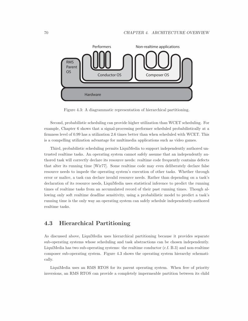
70 CHAPTER 4. ARCHITECTURE OVERVIEW
Hardware
Composer OSConductor OS
Non-realtime applicationsPerformers
RMSParentOS
Figure 4.3: A diagrammatic representation of hierarchical partitioning.
Second, probabilistic scheduling can provide higher utilization than WCET scheduling. Forexample, Chapter 6 shows that a signal-processing performer scheduled probabilistically at afirmness level of 0.99 has a utilization 2.6 times better than when scheduled with WCET. Thisis a compelling utilization advantage for multimedia applications such as video games.
Third, probabilistic scheduling permits LiquiMedia to support independently authored un-trusted realtime tasks. An operating system cannot safely assume that an independently au-thored task will correctly declare its resource needs: realtime code frequently contains defectsthat alter its running time [Wir77]. Some realtime code may even deliberately declare falseresource needs to impede the operating system’s execution of other tasks. Whether througherror or malice, a task can declare invalid resource needs. Rather than depending on a task’sdeclaration of its resource needs, LiquiMedia uses statistical inference to predict the runningtimes of realtime tasks from an accumulated record of their past running times. Though al-lowing only soft realtime deadline sensitivity, using a probabilistic model to predict a task’srunning time is the only way an operating system can safely schedule independently-authoredrealtime tasks.
4.3 Hierarchical Partitioning
As discussed above, LiquiMedia uses hierarchical partitioning because it provides separatesub-operating systems whose scheduling and task abstractions can be chosen independently.LiquiMedia has two sub-operating systems: the realtime conductor (c.f. B.3) and non-realtimecomposer sub-operating system. Figure 4.3 shows the operating system hierarchy schemati-cally.
LiquiMedia uses an RMS RTOS for its parent operating system. When free of priorityinversions, an RMS RTOS can provide a completely impermeable partition between its child
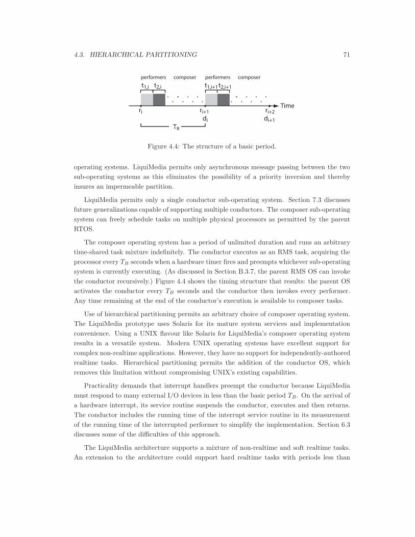
4.3. HIERARCHICAL PARTITIONING 71
Timeri
di di+1
t1,i
TB
performers performers
t1,i+1t2,i+1
ri+1 ri+2
t2,i
TB
composer composer
Figure 4.4: The structure of a basic period.
operating systems. LiquiMedia permits only asynchronous message passing between the twosub-operating systems as this eliminates the possibility of a priority inversion and therebyinsures an impermeable partition.
LiquiMedia permits only a single conductor sub-operating system. Section 7.3 discussesfuture generalizations capable of supporting multiple conductors. The composer sub-operatingsystem can freely schedule tasks on multiple physical processors as permitted by the parentRTOS.
The composer operating system has a period of unlimited duration and runs an arbitrarytime-shared task mixture indefinitely. The conductor executes as an RMS task, acquiring theprocessor every TB seconds when a hardware timer fires and preempts whichever sub-operatingsystem is currently executing. (As discussed in Section B.3.7, the parent RMS OS can invokethe conductor recursively.) Figure 4.4 shows the timing structure that results: the parent OSactivates the conductor every TB seconds and the conductor then invokes every performer.Any time remaining at the end of the conductor’s execution is available to composer tasks.
Use of hierarchical partitioning permits an arbitrary choice of composer operating system.The LiquiMedia prototype uses Solaris for its mature system services and implementationconvenience. Using a UNIX flavour like Solaris for LiquiMedia’s composer operating systemresults in a versatile system. Modern UNIX operating systems have excellent support forcomplex non-realtime applications. However, they have no support for independently-authoredrealtime tasks. Hierarchical partitioning permits the addition of the conductor OS, whichremoves this limitation without compromising UNIX’s existing capabilities.
Practicality demands that interrupt handlers preempt the conductor because LiquiMediamust respond to many external I/O devices in less than the basic period TB. On the arrival ofa hardware interrupt, its service routine suspends the conductor, executes and then returns.The conductor includes the running time of the interrupt service routine in its measurementof the running time of the interrupted performer to simplify the implementation. Section 6.3discusses some of the difficulties of this approach.
The LiquiMedia architecture supports a mixture of non-realtime and soft realtime tasks.An extension to the architecture could support hard realtime tasks with periods less than

72 CHAPTER 4. ARCHITECTURE OVERVIEW
the basic period TB by adding additional sub-operating systems executing as higher prioritypreemptive RMS tasks in LiquiMedia’s parent operating system.
LiquiMedia’s use of hierarchical partitioning permits it to satisfy the principle of processorpartitioning. Non-realtime code can never interfere with the execution of realtime code. Fur-ther, hierarchical partitioning provides different task and scheduling abstractions for realtimeand non-realtime tasks. While this requires developers to learn two different abstractions,they are abstractions for two distinctly different application domains. Non-realtime applica-tions have negligible architectural similarity with realtime applications and the application’sprogramming model should reflect it.
4.4 Realtime Performers
Realtime tasks in LiquiMedia use the performer-style task abstraction (c.f. B.1) for two rea-sons. First, performers are a practical and natural choice for media processing. Second, onlyperformers permit an implementation sufficiently efficient for ultra-fine granularity realtime.
4.4.1 Practical and Natural
The performer task abstraction is practical because examples and programming expertiseexist. This expertise and examples exist because the media generation frameworks (MGF)discussed in Chapter 3 use performer-style tasks. Furthermore, practical use of the LiquiMediaarchitecture involves porting media processing components from an MGF to LiquiMedia. TheMGF components are already written as performers so LiquiMedia’s use of the performer-styletask abstraction minimizes the porting effort.
The performer task abstraction is a natural choice because its combination of atomic andsynchronous execution resembles the mathematical structure of digital signal processing ap-plications [OS94]. Each invocation of a performer processes a single sample in a uniform fixedrate sample stream such as a sequence of video frames or audio samples. Furthermore, ev-ery performer remains synchronized with every other performer so applications can can easilycompose performers together into filter chains.
4.4.2 Efficient
The performer task abstraction is also efficient because performers voluntarily relinquish theprocessor at the end of their execution and thereby reduce the overhead of switching betweenperformers to that of a function call. In contrast, threaded task abstractions have the overheadof a full context switch when switching between tasks. Context switching costs for multimedia
4.5. NON-REALTIME THREADS 73
tasks are increasing as processors incorporate special multimedia execution units. For example,Intel’s MMX multimedia extension adds eight 64-bit registers to the IA32 micro-architecturewhile SSE adds a further eight 128-bit registers [Int99]. VLIW systems take this trend further.
Combining distributed scheduling with the performer task abstraction permits even greaterefficiencies. With distributed scheduling, an application can fix the order of performer exe-cution and hence optimize cache and register usage across performer invocations while stillexposing individual performers to system-wide scheduling. In contrast, application developerscannot control the interleaving of preemptive threads and so can neither optimize cache norregister usage across threads.
4.5 Non-realtime Threads
While performers are an efficient and natural task abstraction for realtime media-generatingtasks, they are not appropriate for long-running non-realtime tasks. Instead, for long runningnon-realtime tasks, LiquiMedia uses the preemptive threading task abstraction. The Liqui-Media prototype uses Solaris as its composer operating system. Consequently it inherits allof Solaris’s design aspects including preemptive threading [Bac86, GC94]. In the LiquiMediaarchitecture, traditional non-realtime applications such as compilers, shells and mail clientsexecute as preemptive threads because, as UNIX’s enduring success clearly demonstrates, thepreemptive thread abstraction is satisfactory for long-running non-realtime applications.
4.6 Conduit IPC
As described in Sections 4.1 and 4.3 above, a LiquiMedia application consists of both per-formers and composer tasks. However, hierarchical partitioning rigidly separates these twodifferent types of tasks to prevent composers from interfering with performer execution. Liqui-Media’s conduit inter-process communication (IPC) facility permits composers and performersto communicate while preserving this partition.
Conduits are an asymmetric one-directional message passing facility with a design inspiredby sockets in UNIX [LMKQ89] and conduits in [NK91]. As shown in Figure 4.5, each conduithas a reader endpoint and a writer endpoint. A task adds messages atomically at the writerendpoint. A task obtains messages atomically at the reader endpoint. A conduit storesmessages internally in a ring buffer.
A conduit’s asymmetry preserves the partition between the composer and conductor sub-operating systems even while permitting communication between them. From the conductor’sview point, a conduit is a non-blocking FIFO and has asynchronous message passing. As a

74 CHAPTER 4. ARCHITECTURE OVERVIEW
next readnow (over)
writtenlast written
next read
now (over)written
next read
Before AfterAction
performer or composer writing to a conduit with space
performer or composer reading from a conduit with elements
performer write to a full conduit
composer write to a full conduit or composer read from an empty conduit
Unchanged,composer blocks
Unchanged,returns error
performer read from an empty conduit
newly written
next read
last written
next read
last written
read value
last written
next read
Figure 4.5: The operation of the conduit IPC mechanism.
4.7. TASK-PARTITIONED PERFORMERS 75
result, the conductor need never wait for a composer thread to add or remove an item froma conduit. Instead, the conductor continues executing without the risk of a priority inversionimposed by synchronous IPC.
From a composer thread’s viewpoint, a conduit has the semantics of a UNIX pipe: acomposer writing to a conduit blocks when the ring buffer is full while a composer readingfrom the conduit blocks when the ring buffer is empty. These semantics are a natural choicefor ease of software development given that LiquiMedia’s composer OS is a flavour of UNIX.
To make it possible to write library code usable in both performer and composer tasks,conduits can also be used for performer to performer and composer to composer communica-tion. When used for performer to performer communication, both of a conduit’s endpointshave have non-blocking FIFO semantics while a conduit acts as a UNIX pipe for composer tocomposer communication.
Besides permitting communication between sub-operating systems without sacrificing thepartition between them, conduits are also a practical IPC mechanism for multimedia appli-cations such as the LiquiMedia audio player. Described further in 6.2, the LiquiMedia audioplayer combines an audio decompression composer with filter and output performers. A con-duit carrying audio samples was the ideal communication mechanism between these tasksbecause it provided the “best-effort” synchronization needed between a non-realtime (andnon-synchronous) composer and synchronous realtime performers.
4.7 Task-partitioned Performers
The conductor uses the instantaneous admission control mechanism discussed in Section 4.9to provide a permeable task partition between performers. Before executing a performer, theconductor verifies that the basic period contains sufficient remaining time for its execution. Ifinsufficient time remains because previously executed performers ran longer than predicted,the conductor defers the performer’s execution.
As a result, every performer must be prepared to address the situation where the conductorhas not executed it for one or more previous basic periods. The conductor informs eachperformer on invocation of the number of preceding basic periods in which the performer hasnot been invoked. Most MGF applications have an obvious response such as skipping framesor advancing the step size of a simulation.
4.8 Schedule Graph
The conductor uses a generalization of distributed scheduling that I call a scheduling graph. Aschedule graph represents the schedule as a DAG where a node is a performer and its outbound
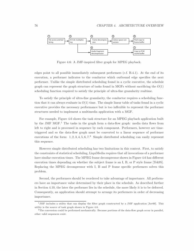
76 CHAPTER 4. ARCHITECTURE OVERVIEW
A/V de-multiplex-ing
File access and buf-fering
Frame decompres-sion
Audio fragment decompression
Colour space con-version
Pixel copy to frame-buffer
Copy to PCM sound buffer
1 2 3 5 6
74
Figure 4.6: A JMF-inspired filter graph for MPEG playback.
edges point to all possible immediately subsequent performers (c.f. B.4.1). At the end of itsexecution, a performer indicates to the conductor which outbound edge specifies the nextperformer. Unlike the simple distributed scheduling found in a cyclic executive, the schedulegraph can represent the graph structure of tasks found in MGFs without sacrificing the O(1)scheduling function required to satisfy the principle of ultra-fine granularity realtime.
To satisfy the principle of ultra-fine granularity, the conductor requires a scheduling func-tion that it can always evaluate in O(1) time. The simple linear table of tasks found in a cyclicexecutive provides the necessary performance but is too inflexible to represent the performerstructures needed to implement a multimedia application with a MGF.
For example, Figure 4.6 shows the task structure for an MPEG playback application builtby the JMF MGF.1 The tasks in the graph form a data-flow graph: media data flows fromleft to right and is processed in sequence by each component. Performers, however are time-triggered and so the data-flow graph must be converted to a linear sequence of performerexecutions of the form: 1, 2, 3, 4, 5, 6, 7.2 Simple distributed scheduling can easily representthis sequence.
However simple distributed scheduling has two limitations in this context. First, to satisfythe constraints of statistical scheduling, LiquiMedia requires that all invocations of a performerhave similar execution times. The MPEG frame decompressor shown in Figure 4.6 has differentexecution times depending on whether the subject frame is an I, B, or P style frame [Tek95].Replacing the MPEG decompressor with I, B and P frame specific performers solves thisproblem.
Second, the performers should be reordered to take advantage of importance. All perform-ers have an importance value determined by their place in the schedule. As described furtherin Section 4.10, the later the performer lies in the schedule, the more likely it is to be deferred.Consequently, an application should attempt to arrange its performers in order of decreasingimportance.
1JMF includes a utility that can display the filter graph constructed by a JMF application [Jav00]. This
utility is the source of task graph shown in Figure 4.6.2The conversion could be performed mechanically. Because portions of the data-flow graph occur in parallel,
other valid sequences exist.

4.8. SCHEDULE GRAPH 77
A/V
de-
mul
tiple
x-in
gFi
le a
cces
s an
d b
uf-
ferin
gFr
ame
typ
e de
ter-
min
atio
nB
fram
e de
com
-p
ress
ion
I fra
me
deco
m-
pre
ssio
n
P fr
ame
deco
m-
pre
ssio
n
Aud
io fr
agm
ent
deco
mp
ress
ion
Col
our s
pac
e co
n-ve
rsio
nPi
xel c
opy
to
fram
e-b
uffe
rC
opy
to P
CM
so
und
buf
fer
Pre-
roll
or s
us-
tain
ed p
lay
A/V
de-
mul
tiple
x-in
gA
udio
frag
men
t de
com
pre
ssio
n
A/V
de-
mul
tiple
x-in
g
3 8 10
1
3 83
11
5 62
7
94
Figure 4.7: The final schedule graph for a LiquiMedia MPEG player.
78 CHAPTER 4. ARCHITECTURE OVERVIEW
Figure 4.7 shows the final form of the example. In it, the performers are in order ofdecreasing importance with audio decompression favoured over video decompression. Also,the graph features the paths necessary to handle both steady-state playback and pre-roll. Thedirected graph contains multiple paths where each path defines a possible performer executionsequence:3
{1, 2}{1, 3, 4, 5, 2}
{1, 8, 3, 9, 4, 5, 2}{1, 8, 3, 9, 4, 6, 2}{1, 8, 3, 9, 4, 7, 2}
{1, 10, 8, 3, 11, 9, 4, 5, 2}{1, 10, 8, 3, 11, 9, 4, 6, 2}{1, 10, 8, 3, 11, 9, 4, 7, 2}.
Such a task graph cannot be represented by the cyclic executive’s linear list of tasks andinstead requires the more general schedule graph representation.
Fortunately, this more general representation does not increase the overhead of the conduc-tor’s scheduling function. An adjacency list representation for the schedule permits the conduc-tor to contain an O(1) implementation of the scheduling function [CLR90]. The adjacency-listrepresentation provides both a flexible schedule structure and the efficiency required by theprinciple of ultra-fine grain realtime.
The above example also demonstrates a general-purpose strategy for reducing performervariance. Developers should sub-divide a large monolithic performer such as performer 3 inFigure 4.6 into the multiple simpler performers {4, 5, 6, 7} found in Figure 4.7 whenever themonolithic performer chooses to execute one of several different functions in a basic period.A multi-function performer’s variance is the sum of squares difference between its averagerunning time and the running times of the individual component functions. Dividing themulti-function performer into separate performers lowers the total variance and better exposesthe application’s structure for more advantageous scheduling.
4.9 Statistical Admission Control
LiquiMedia satisfies the principle of modularity with its two ESAC admission control mecha-nisms. The scheduler uses the lifetime admission control mechanism to insure that an entire
3The graph permits two additional paths: {1, 3, 4, 6, 2} and {1, 3, 4, 7, 2}. Because MPEG playback must
begin on an I frame, these paths are never executed.

4.9. STATISTICAL ADMISSION CONTROL 79
schedule graph (the average of many performers) has sufficient firmness while the conductoruses instantaneous admission control in the instant before invoking a performer to insure thatthe performer has a sufficient probability of executing in realtime.
4.9.1 Lifetime Admission Control
The schedule graph provides the foundation for both admission control mechanisms. Theconductor executes performers as specified by the current schedule. Each performer node in thisgraph includes a probabilistic estimate of the performer’s running time. The conductor usesthis estimate for its instantaneous admission control mechanism. Should the conductor admita performer and the performer execute successfully, the conductor also records the statisticalinformation described in Section B.3.6 in the performer’s node in the schedule graph.
The scheduler’s lifetime admission control mechanism regularly re-verifies that the currentschedule has at least the required minimum probability of realtime execution. During thecourse of this re-verification, it closes the feedback loop between the conductor’s collection ofstatistical information and its use of estimates of a performer’s running time (c.f. B.4.6).
The scheduler also invokes its admission control mechanism in response to an applicationrequesting an alteration of the schedule graph. In this case, the scheduler first constructs a newschedule combining all the unaltered sub-graphs of the current schedule with the application’ssubmission and then admission tests the new schedule. The scheduler combines applicationsub-graphs in their order of submission — placing the newest sub-graph last. Should thenew schedule prove admissible, the scheduler passes it to the conductor and the new schedulebecomes the current schedule at the conductor’s earliest convenience.
The admission control test has the same four stages regardless of whether the scheduler isapplying it to a newly created schedule or re-testing the conductor’s current schedule. First,the scheduler computes a probabilistic bound on each performer’s running time and attachesit to the subject schedule graph. Second, the scheduler uses these per-performer estimatesto compute a probabilistic bound on the running time of each path in the schedule graph.Third, the scheduler tests that the estimated running times of all such paths remain less thanthe duration of a basic period and, if they do, passes the schedule graph to the conductor.Otherwise, the subject schedule has experienced a lifetime admission failure and the schedulerinvokes the fourth stage: it removes the least important performers from the schedule andrepeats the admission process on the now reduced subject schedule.
In the first stage, the scheduler computes a probabilistic bound on each performer’s runningtime. It estimates a performer’s running time with Chebyshev’s inequality because Cheby-shev’s inequality holds regardless of the distribution of the performer’s running time [WM78].Section B.2 presents the mathematical details.
80 CHAPTER 4. ARCHITECTURE OVERVIEW
Use of Chebyshev’s inequality requires the mean and standard deviation of a performer’srunning time. As described in Section B.3.6, the scheduler uses Chan et al.’s pair-wise al-gorithm to compute these summary statistics from the invocation count, sum of performerrunning times and sum of squared performer running times [CGL83]. The conductor col-lects these values by measuring a performer’s actual running time on every invocation with ahardware cycle counter.
An un-executed performer does not have collected statistical information. Consequently,LiquiMedia requires that applications provide estimates of each performer’s standard deviationand mean running time. The admission control mechanism uses these values when admissiontesting a schedule containing new performers.
In the second stage of the admission control test, the scheduler enumerates the pathsthrough the schedule graph via depth-first graph traversal. For each path, it combines theper-performer estimates as described in Section B.4.5 and estimates the total running time ofthe path.
In the third stage, the scheduler verifies that all of the previously calculated per-pathestimates are less than the basic period. Finally, only if one or more of the path estimatesexceed the basic period will the scheduler enter the fourth stage: resolving a lifetime admissionfailure by removing the last-most performer from each inadmissible path until the schedulebecomes admissible.
A lifetime admission failure can occur in three situations. First, an application’s initialestimate of its performers’ running times can show that these un-executed performers areinadmissible. Second, while the scheduler may have admitted new performers based on an ap-plication’s initial estimate of their running time, they may not be admissible once the schedulerhas computed estimates of their running times from conductor-collected measurements. Third,a long-running performer may suddenly begin to take significantly longer to execute.
A lifetime admission failure can be severe because correcting it can interrupt one or moreexisting realtime streams. However most such failures are harmless because they are causedby the first two situations described above. In the first situation, the affected performers havenever executed and so removing them from the schedule does not interrupt an existing realtimestream.
In the second situation, the scheduler admission tests and removes the affected performersfrom the schedule before the user perceives them as realtime stream. The lifetime admissioncontrol mechanism can test a schedule within a user’s 200 millisecond segregation thresholdbecause, as shown in Section 6.5.3, the conductor provides the scheduler with per-performersummary statistics sufficiently accurate for admission testing within 10 basic periods or 130milliseconds.
Unfortunately, the third situation under which a lifetime admission failure can occur doesdisrupt established streams. In the third situation, a performer embedded inside the current

4.10. INSTANTANEOUS ADMISSION CONTROL 81
t1,i predicted t7,i
truncated t7,i'
Timeri ri+1
Figure 4.8: An example of an overtime scheduling error: performer 7 has not finished executingat the end of the basic period.
schedule increases its running time or variance to such an extent that the schedule becomesinadmissible. For example, assume that performer 9 in Figure 4.7 contains a programmingerror that causes its execution variance to increase in proportion to the number of displayedframes. Eventually, the error renders the performer inadmissible and the scheduler will removethe sub-path {9, 4, 7, 2} and consequently interrupt the video stream.
However, the performers {1, 10, 8, 3, 11} continue to operate and so the video’s audio streamremains unaffected. This example shows how LiquiMedia provides importance: performersearly in the schedule graph are preserved at the expense of later performers. Because aperformer’s importance is tied to its position in the schedule graph, an application can easilyspecify the relative importance of its performers with its schedule graph.
The lifetime admission failure is one of three scheduling errors that LiquiMedia can en-counter. The other two are overtimes and deferrals. Figure 4.8 shows an example of anovertime: performer p = 7 has not completed executing at the beginning of the next basicperiod. When this occurs, the conductor suspends the execution of performer p, notifies viaconduit any interested composer threads and does not attempt to execute p in subsequentbasic periods. Overtimes are LiquiMedia’s most severe type of scheduling error because theyalways interrupt the generation of a realtime stream.
4.10 Instantaneous Admission Control
Because overtimes are so serious, the conductor uses its instantaneous admission control mech-anism to substitute a deferral for the more serious overtime scheduling error. A deferral occurswhen the conductor’s instantaneous admission control mechanism detects and avoids a poten-tial overtime. As shown in Section 6.5.2, this mechanism eliminates all overtimes in schedulescomprised of standard test performers.
Figure 4.9 shows an example. Here, performer 7 has less than probability Pc of executingbefore the end of basic period j so the conductor defers its execution.
The conductor implements the instantaneous admission control mechanism (c.f. B.3.5).Before invoking a performer, it tests if the the time remaining in the current basic period

82 CHAPTER 4. ARCHITECTURE OVERVIEW
t1,j
tc
lt(7,Pc)
Timerj rj+1
Figure 4.9: An example of a deferral. The shaded blocks indicate the running times of per-formers 1 . . . 6 whose sum exceeds lt(7, Pc) — the latest Pc-likely start time of performer 7.
exceeds the Pc-likely estimate of the performer’s running time. Only if the time remainingexceeds the estimate will the conductor invoke the performer. The scheduler computes aperformer’s estimated running time each time that it re-verifies the schedule.
The conductor counts the number of overtimes taken by any performer. During re-verification, the scheduler suspends performers which have experienced an unacceptable num-ber of overtimes. As with all other circumstances where a performer is suspended, LiquiMedia’sscheduler notifies interested composers.
Besides illustrating a deferral, Figure 4.9 also shows why LiquiMedia ties importance to aperformer’s position in the schedule. The later the conductor executes a performer in the basicperiod, the more likely it is that the performer experiences a deferral or an overtime schedul-ing error because with each successive performer executed, the time remaining to execute aperformer decreases. As a result, while the admission control mechanisms insure that everyexecuted performer has at least a firmness of Pc, earlier performers have a higher probability ofexecuting successfully. LiquiMedia takes advantage of this property to provide per-performerimportance simply by controlling the structure of the schedule graph.
Deferrals are the least serious scheduling error because they only briefly interrupt streamgeneration. For example, a single dropped video frame passes unnoticed and audio hardwarehas sufficient buffering to hide a single deferral in a performer generating an audio stream.4
The instantaneous admission control mechanism helps LiquiMedia to support higher real-time loadings without damaging the user experience. As shown in Section 6.5.2, the instan-taneous admission control mechanism eliminates overtimes at schedule loadings which wouldotherwise always experience them. By converting overtimes into deferrals, LiquiMedia canexecute highly loaded schedules without subjecting users to the unpleasant gaps in a realtimestream caused by performer overtimes.
4For example, the SGI VisualWorkstation has an 8kB hardware audio buffer which holds approximately 3.5
basic periods of CD quality audio [Sil99].
4.11. SATISFIES FUNDAMENTAL PRINCIPLES 83
4.11 Satisfies Fundamental Principles
LiquiMedia is a multimedia operating system. Chapter 1 defines four principles that a mul-timedia operating system must satisfy: the principle of processor partitioning, synchronousrealtime, modularity and ultra-fine granularity realtime. LiquiMedia satisfies these principleswith a unique combination of the design aspects introduced in Chapter 2, which support oneanother in creating a novel multimedia operating system architecture.
First, LiquiMedia combines hierarchical partitioning with asynchronous message passingIPC to satisfy the principle of partitioning. The parent RMS operating system required byhierarchical partitioning imposes a rigid partition between realtime and non-realtime codewhile asynchronous IPC eliminates partition-violating priority inversions when the conductorand composer sub-operating systems communicate.
Second, LiquiMedia satisfies the principle of synchronous realtime execution with hierar-chical partitioning, performer tasks and global time-triggered externalization. Hierarchicalpartitioning enables different task and scheduling models for performers and composers. Allperformers are synchronized with one another and with a global clock. Only by writing and sub-mitting a performer can an application developer have code execute in realtime. Consequently,developers cannot write realtime code without explicitly acknowledging that it operates withinan isochronous invocation framework that is bound to external time.
Third, LiquiMedia satisfies the principle of modularity through a combination of statisticaladmission control, distributed scheduling and hierarchical partitioning. The principle of mod-ularity requires that LiquiMedia support the execution of independently authored realtimeand non-realtime applications.
Supporting independently authored non-realtime applications is easy. Thanks to hierarchi-cal partitioning, the LiquiMedia architecture can include a general purpose non-realtime childoperating system. Most such operating systems, including UNIX variants, WindowsNT andVMS, support the execution of independently authored non-realtime applications.
Supporting independently authored realtime applications is more difficult. Satisfying therealtime constraints of independently authored realtime code requires an admission controlmechanism. Admission control mechanisms need to know the running times of realtime ap-plications. But, independently authored realtime applications cannot be trusted to accuratelyrepresent their resource needs — particularly if an accurate representation excludes the appli-cation from executing at all.
LiquiMedia solves this dilemma by using statistical inference to predict the running times ofperformers. However such calculations are expensive. Using distributed scheduling separatesthe production of a schedule from its use for the dispatching of tasks and so satisfies theprinciple of modularity without jeopardizing the conductor’s efficiency.
84 CHAPTER 4. ARCHITECTURE OVERVIEW
Finally, LiquiMedia satisfies the principle of ultra-fine granularity realtime with the sta-tistical admission control, performer and distributed scheduling design aspects. As shown inSection 6.4, performer-style tasks are at least 9.48 times more efficient than threads despite theoverhead of the conductor’s admission control facilities. Instantaneous admission control per-mits LiquiMedia to provide an efficient and almost impermeable partition between performers.Distributed scheduling efficiently supports large numbers of performers.
Per-performer dispatch overhead is O(1) when running a fixed set of realtime tasks. Sched-ule creation and modification costs in LiquiMedia are high but this is not a problem fortwo reasons. First, in actual usage situations, infrequent schedule management operations areamortized over many basic periods of performer dispatch. Second, schedule management oper-ations are most frequent during application startup. Here, dynamic linking and demand-pagedloading dwarfs the time cost of schedule management.
LiquiMedia combines the following design aspects: hierarchical partitioning, global time-triggered externalization fixed performer-style tasks, distributed scheduling, statistical ad-mission control and atomic task IPC. These design aspects work together to let LiquiMediaimplement the fundamental principles of a multimedia operating system.
4.12 Summary
Unlike the solutions discussed above, LiquiMedia’s novel combination of design aspects satisfiesall four of the fundamental principles. First, LiquiMedia combines hierarchical partitioning,performer-style tasks and atomic task IPC to satisfy the principal of partitioning. Second, itsatisfies the principle of synchronous realtime execution with globally externalized performer-style tasks. Third, LiquiMedia satisfies the principle of modularity with its admission controlmechanism. Rather than trusting independently-authored performers to correctly declare theirrunning times, LiquiMedia estimates a performer’s running time from its past execution anduses this estimate to accept or reject the scheduling of a performer. Lastly, LiquiMedia sat-isfies the principle of ultra-fine granularity realtime with its use of the light-weight performerand distributed scheduling design aspects. Only distributed scheduling performer-style taskspermit an operating system to efficiently interleave the operation of a large number of tinyrealtime fragments. Other operating systems either provide fine granularity realtime executionor support independently authored realtime code but not both. Only LiquiMedia satisfies bothprinciples at once.
Chapter 5
Implementation
The previous chapter provided an overview of LiquiMedia’s architecture. This chapter dis-cusses the implementation of the liqui prototype. I built liqui as an experimental platformto test LiquiMedia’s central features: fine grain realtime fragments, statistical admission con-trol and feedback-driven schedule refinement.
5.1 Extending Solaris
Building liqui on top of Solaris 2.6 reduced implementation time and provided more timefor testing the prototype’s implementation of the four principles of a multimedia operatingsystem. While the alternative of developing for the naked hardware is an interesting challenge,re-implementing code such as an RMS scheduler or thread library adds no academic contri-bution. Instead, LiquiMedia uses the Solaris static priority realtime facilities to provide itsrate monotonically scheduled (RMS) parent OS and Solaris time-shared UNIX processes forits composer operating system.
The Solaris 2.6 kernel has the preemptive thread task abstraction [Sun95b]. The Solarisdocumentation calls these threads light weight processes (LWP).1 Multiple LWPs may share asingle set of memory mapping resources.
The kernel schedules LWP execution with a hierarchical scheduler. Solaris reserves thetop half of the available priority levels for realtime LWPs. These LWPs have the realtimescheduling class. Solaris provides strict RMS schedule discipline for LWPs using these prioritylevels. The kernel does not provide priority inheritance so is vulnerable to priority inversion. Atraditional UNIX decaying priority scheduler dynamically assigns the remaining priority levelsto non-realtime LWPs in the time-shared scheduling class [Sun95c].
1Solaris also has a higher level wrapper for the LWP that the documentation refers to as a thread.
85

86 CHAPTER 5. IMPLEMENTATION
The kernel operates in a reentrant fashion for non-realtime LWPs. Multiple non-realtimeLWPs can simultaneously block in kernel context. The situation for realtime LWPs is moreproblematic. Portions of the kernel must operate below Solaris’s lowest realtime priorities.When combined with the kernel’s lack of priority inheritance, this significantly limits theusability of Solaris’s realtime threads.
Despite these limitations, LiquiMedia maps closely to the structure of Solaris. Solaris’s twoscheduling classes provides a hierarchical partition. The conductor executes inside a SolarisLWP with the realtime scheduling class. Further, Solaris’s time-shared scheduling class andthreaded task abstraction handily served as liqui’s non-realtime composer child OS whereLiquiMedia composer threads run as non-realtime Solaris LWPs.
Building liqui on top of Solaris greatly reduced development effort. However, the resultingloss of low-level control imposed some practical difficulties. The most significant issues wereinterrupt handling, timing variance, Solaris’s absence of priority inheritance and sharing accessto hardware devices between realtime and non-realtime LWPs.
Many hardware devices have maximum service latencies that are impossible to handleusing performer-polling. Consequently, as discussed in 4.3, LiquiMedia permits interrupts topreempt the conductor. However, interrupt handling code poses a difficult problem: it stealsexecution time from performers. There are two possible responses. First, include the runningtime of interrupt handling code in a a performer’s execution time. Second, pause the countersused to measure a performer’s running time during the execution of interrupt handling code.
Solaris does not permit implementing the second mechanism thought it might be possibleto alter the Solaris interrupt dispatch code to implement this mechanism. Consequently, Liqui-Media includes the contribution of interrupt handlers in performer running times. Chapter 6shows that even a performer with a constant running time has a sizable execution time vari-ance. Interrupts cause some of this variance with rest caused by cache misses and TLB misses.The per-performer execution time variance limits liqui’s maximum firmness. A version ofLiquiMedia running on the naked hardware would support greater firmness levels.
Not only is Solaris incapable of pausing the performance registers during interrupts but itdoes not even provide a mechanism by which the conductor can efficiently disable interrupts.Consequently, because it is always enabled, the basic period interrupt can arrive at any pointin the conductor’s execution. As a result, the conductor in liqui must handle all of thereentrant cases identified in B.3.7.
Solaris 2.6’s lack of a priority inheritance mechanism also posed an implementation chal-lenge. The liqui conduit library requires mutex-protected access to conduit data structures.These mutexes are shared between non-realtime application LWPs and the realtime conductorLWP. Consequently, a naive implementation of liqui experiences a priority inversion if thebasic period interrupt occurs while a composer thread holds the conduit mutex. The conduitlibrary solves this problem with a priority inheritance mechanism.
5.1. EXTENDING SOLARIS 87
Interfacing with devices was the final implementation challenge imposed by Solaris. Por-tions of the Solaris kernel execute at a lower priority than LWPs in the Solaris realtime priorityclass. Consequently, use of kernel services such as those necessary to handle a breakpoint canalso cause a priority inversion. Unfortunately, the system documentation inadequately de-scribes the priority inversion safety of the various kernel services and device drivers.
Fortunately, it is possible to access both the sound device and the low level framebufferdevice in realtime. Realtime access to these devices is sufficient for performers to generatemultimedia streams for both the modalities of vision and hearing. Realtime access to theframebuffer device also enabled liqui to use the vertical retrace interrupt for its basic periodinterrupt.
The vertical retrace is an ideal source of basic period interrupts for three reasons. First, theinterrupt is isochronous. Second, the rate of the interrupt (by design) exceeds the minimumrate required for a human’s visual modality to fuse separate video frames into a continu-ous visual stream [Wic84]. Third, use of the interrupt automatically synchronizes performerexecution with the refresh of the display.
Building liqui on Solaris sacrificed low-level hardware and operating system control. Thisloss of low-level control caused the implementation difficulties described above. Despite this,building liqui on top of an existing operating system was the correct decision for three reasons.
First, by building on top of an existing operating system, I finished coding more quickly.All modern operating systems contain large amounts of common code such as number to stringconversion, stack frame setup and context switching. These functions are not academicallyinteresting and yet require correct implementation for the operating system to function. Con-sequently, liqui builds on the facilities provided by Solaris rather than re-implementing thesenecessary but uninteresting functions.2
Second, implementing LiquiMedia as an extension to Solaris provides a better demon-stration of the principle of processor partitioning than building an operating system on nakedhardware. The principle separates realtime and non-realtime code by hosting them in indepen-dent sub-operating systems. Successfully combining independently-developed sub-operatingsystems — Solaris and liqui for example — more convincingly shows the principle of parti-tioning’s strength: separation of different independent scheduling domains.
Third, LiquiMedia’s admission control mechanism must operate correctly despite back-ground system activities that increase the variance of performer execution. Solaris adds con-siderable variance to performer execution, compared to a native implementation of LiquiMedia.Consequently, building liqui on Solaris more rigorously tests LiquiMedia’s scheduling tech-niques than does a native implementation.3
2In retrospect, it might have been better to implement the prototype as an extension to Linux. However,
at the time that I began the implementation, the Linux kernel lacked preemption.3A prototype running directly on the underlying hardware could address this with artificial sources of

88 CHAPTER 5. IMPLEMENTATION
Building liqui as an application on top of Solaris simplified the implementation. Further,augmenting Solaris actually resulted in a superior demonstration of LiquiMedia’s value byshowing the importance of the principle of processor partitioning and the admission controlmechanism’s robust handling of performer variance.
5.2 Implementation Structures
This section describes various implementation challenges encountered while implementingliqui, their solutions and the limitations that remain.
5.2.1 Conduits
Conduits are asymmetric non-blocking FIFOs as described in Section 4.6. liqui’s conduitscan contain only objects that can be written in a single assembly language statement. Thisrestriction bounds the time needed to read or write a conduit. liqui requires this boundbecause all conduit accesses occur inside a mutex required to insure that conduit position andcurrent value are accessed atomically. Preprocessor macros and an abusive use of C’s typecasting facilities makes conduits generic. Section 7.2.3 discusses some possible improvementsfor the conduit mechanism.
5.2.2 Exception Handlers
liqui has a structured exception handling mechanism. The exception handling mechanismunifies the delivery of UNIX signals and LiquiMedia-specific errors to performers and com-posers. I implemented this mechanism for three reasons. First, the priority inheritance mech-anism required centralizing UNIX signal handling. Second, the exception framework permitsasynchronous termination of a Solaris LWP. Finally, the exception framework simplified errorhandling in liqui applications.
liqui includes a a priority inheritance system to eliminate priority inversion deadlocksbetween composer threads and the conductor. The priority inheritance system captures allasynchronous UNIX signals to insure that an interrupted composer thread clears the conduitmutex before the conductor attempts to acquire it. Consequently, liqui routes all asyn-chronous signals including the basic period interrupt through the priority inheritance system.liqui accumulates signal notifications and uses the exception mechanism to dispatch themsynchronously.
variance. However, a production OS running real task loads provides a more realistic source of execution
variance.

5.2. IMPLEMENTATION STRUCTURES 89
Solaris provides no easy way to asynchronously halt the execution of a Solaris LWP. Conse-quently, all composer threads in liqui run under an exception dispatch wrapper. This permitsliqui to terminate all the threads comprising a single application without restarting. The ex-ception framework also safely terminates an application thread if it generates a synchronousfault.
Finally, the structured exception mechanism simplified the development of applications.With an exception handling framework in place, much of the error checking needed in tra-ditional UNIX C coding became unnecessary. Moreover, the structured mechanism providedan error detection and handling mechanism consistent across both realtime and non-realtimecode.
5.2.3 Applications
liqui cannot execute normal Solaris applications. Instead, each application consists of ashared library containing its performers and composers. liqui initiates an application byhaving the dynamic linker load the application’s shared library and then invoking the app main
entry point in a new composer thread.
The Solaris dynamic linker provides on-demand loading of an application’s components.liqui fully resolves an application’s dependencies on load so that a performer’s first invocationdoes not invoke the dynamic linker.
Both the principles of partitioning and modularity require memory protection bound-aries between applications. LiquiMedia’s scheduling approach is compatible with traditionalhardware-enforced memory protection boundaries. However, the overhead of hardware mem-ory protection is incompatible with the principle of ultra-fine granularity realtime fragments.
Consequently, I designed liqui with the goal of extending it into a realtime Java Vir-tual Machine (JVM) where the JVM’s software memory protection mechanism would providememory protection boundaries between applications.4 Anticipating this extension, all liquiapplication components operate inside a single shared memory space. However, while a viola-tion of the principle of modularity, I wrote most of liqui’s test applications in C because thissimplified their development.
5.2.4 Memory Management
LiquiMedia must reclaim memory allocated by applications with an automatic storage man-agement for two reasons. First, LiquiMedia cannot rely on independently-authored code to
4As discussed in Appendix D, LiquiMedia Inc. used liqui to build a prototype of such a JVM that provides
realtime execution of independently-authored Java code fragments.
90 CHAPTER 5. IMPLEMENTATION
include the function calls needed to relinquish previously allocated storage so satisfying theprinciple of modularity requires automatic storage management. Second, the conductor cansuspend a performer midway through its execution and a suspended performer’s heap alloca-tions can only be recovered by an automatic storage management system.
Two techniques exist to automatically recover previously allocated storage in a sharedheap: reference counting and garbage collection. Reference counting is incompatible with theprinciple of partitioning because reference counting requires every access to heap memory tocontend for a lock on the count. Consequently, LiquiMedia must use some form of garbagecollection.
Garbage collection does not solve all storage reclamation problems in a multi-threadedenvironment. A conservative collector thread must implement a write barrier while tracingin-use storage [JL96, Wil96]. An incremental collector must implement a read barrier on theheap. Fortunately, the performer task abstraction simplifies the implementation of either kindof barrier and provides a well-defined structure for root finding.
On a single processor machine, running the collector from the conductor provides theappropriate read or write barrier. Moreover, the atomic execution property of the performertask abstraction insures that the root set consists only of the stack contents of the (suspended)composer threads and any per-application writable static space.
Writing an incremental garbage collector is beyond the scope of this thesis. Consequentlyliqui allocates memory with an instrumented version of the allocation interfaces defined bythe Boehm-Demers collector [Boe04]. The Boehm-Demers collector in fast-halt mode canrun immediately after conductor execution in each basic period. However, liqui does notcompletely implement this feature because its peak heap size did not justify the additionaldevelopment effort.
5.2.5 Timing and Measurement
LiquiMedia requires an efficient and accurate timer. The conductor reads the current timetwice for each performer invocation. Consequently, satisfying the principle of ultra-fine gran-ularity requires that a timer access have as small an overhead as possible. The conductorcomputes each performer’s statistical profile from the values of these timer accesses. Conse-quently, an inaccurate timer invalidates LiquiMedia’s admission control mechanism.
To simplify the implementation, liqui uses Solaris’s gethrtime function to measure per-former execution time. The gethrtime function returns the number of nanoseconds sincesystem boot. As shown in Section 6.4, the 545ns running time of gethrtime is sufficientlysmall to satisfy the principle of ultra-fine granularity realtime.

5.3. IMPLEMENTATION STRATEGY 91
5.3 Implementation Strategy
liqui is divided up into components: structured exception handling, performer objects, con-duits, schedule graph management, the scheduler, the conductor, statistics functions, messagelogging and application loading. Each component was tested in isolation before integrationinto the liqui system.
Each core component has a matching test harness and unit tests. The harnesses werenecessary because many of the components are tightly coupled. For example, as discussed inAppendix B, the scheduler has a complex interaction with the conductor. Consequently, eachtest harness implemented enough of a component’s dependencies to permit unit testing thecomponent in isolation.
LiquiMedia’s operation is non-deterministic and so it is difficult to distinguish betweenoutliers caused by unlikely but correct behaviour and outliers caused by programming errors.Consequently, I also performed a sequence of integration tests to show that the componentsoperating in combination implemented the necessary architectural features from Appendix B.Appendix F lists these tests.
Each integration test had the same structure: a testing composer established an initialstate of the system by directly modifying liqui’s internal data structures and then mutatedthe system. Test results were verified manually. Most integration tests were executed under adebugger with the conductor configured to run a fixed number of basic periods in non-realtime.In retrospect, automatic regression testing would have been helpful.
5.4 The Scheduler Simulator
I implemented a simulator for LiquiMedia’s non-realtime scheduler. The simulator executedthe scheduler’s average-context admission control algorithm and numerical algorithms on awide-variety of test schedules. All schedules were comprised of standard test performers. Eachschedule’s statistical profile data was sampled from liqui’s per-performer execution traces.Consequently, even the synthetic schedules had statistically possible and realistic executiontraces.
The simulator evaluated portions of LiquiMedia that do not execute in realtime. Con-sequently, the simulation neither has nor requires time-accurate operation. It simply takesstatistical profile data and performs admission control decisions in an identical fashion to theactual scheduler.
The simulator provides a superior evaluation of the scheduler than is possible with liqui
for two reasons. First, because it does not operate at the behest of a realtime conductor, itcan admission-test many more schedules per unit time than liqui’s implementation of the

92 CHAPTER 5. IMPLEMENTATION
scheduler. Second, the simulator can test scheduler operation under conditions that cannot bereproduced in realtime.
5.5 Summary
This chapter has described the implementation of the LiquiMedia prototype liqui and simula-tor. liqui is implemented above Solaris for two reasons. First, building on Solaris economizedthe implementation effort by requiring only the development of LiquiMedia’s unique contri-bution. Second, building on Solaris showed that existing operating systems can be retrofittedwith LiquiMedia-style support for multimedia applications. LiquiMedia’s non-realtime sched-uler is both implemented in liqui and separately in a simulator. The simulator permittedevaluating the scheduler’s operation under conditions not reproducible in realtime.
I implemented these two components to demonstrate that the LiquiMedia architecturesatisfies the four principles of a multimedia operating system described in Chapter 1. Chapter 6presents the results of experiments performed with liqui and the simulator which demonstratethat LiquiMedia does satisfy the four principles.

Chapter 6
Performance Measurements
The thesis presents the architecture of the LiquiMedia operating system and its prototypeimplementation liqui. Chapter 4 reasoned that any bug-free implementation of LiquiMedia’sarchitecture, like liqui, satisfies the four principles of a multimedia operating system presentedin Chapter 1. The performance tests discussed in this chapter confirm this reasoning: liquioperates successfully as designed on a range of typical cases. These tests also quantify thepenalties imposed by a real implementation on a possibly unrealizable ideal.
6.1 Apparatus and Methodology
This section describes the experimental software and methodology. The performance testscan be categorized by their goal. First, most of the tests discussed below provide a pass/failconfirmation of the reasoning behind LiquiMedia’s design by showing that liqui operatessuccessfully on a range of typical cases. Second, the remainder of the tests measure liqui’sperformance and compare it to previous approaches.
6.1.1 Metrics
Both kinds of tests use three important metrics. They are defined here.
Loading
A loading is a fraction of a basic period. liqui measures performer running timesin nanoseconds. Because the size of these numbers makes them cumbersome, thischapter specifies performer running times and derived quantities as loadings.
A schedule loading is the fraction of a basic period consumed by executing the per-formers that comprise a path through the schedule and is the sum of each executed
93

94 CHAPTER 6. PERFORMANCE MEASUREMENTS
performer’s loading. Note that liqui cannot support schedule loadings of 1.0 becauseof the time consumed by the conductor’s overhead.
Firmness Pc
Firmness is an input to the scheduler that specifies the probability that a performer’sactual running time is less than the upper bound computed by the scheduler. Sec-tion B.2 provides a formal definition. For example, a pure RMS operating systemprovides a firmness of 1.0.
Expected Utilization
The ratio of a performer’s mean execution time to the execution time allocated to itby a scheduler. Expected utilization (EU) precisely specifies the processor resourcesacrificed by the provision of realtime scheduling. The LiquiMedia scheduler computesa statistical estimate stat(p) of a performer’s running time so the expected utilizationu(stat(p)) after executing performer p for i basic periods is
u(stat(p)) =mp,i
stat(p).
This chapter compares LiquiMedia to operating systems that allocate processor re-sources using the worst case execution time (WCET). In this case, the expectedutilization u(wcet(p)) is
u(wcet(p)) =mp,i
wcet(p),
where wcet(p) is the largest execution time of performer p in any invocation.
It is impossible to determine wcet(p) without knowing the probability distributionfunction (PDF) of performer p. Consequently, this chapter approximates wcet(p)with the sample maximum
wcet(p) ≈ maxi=1,...,n
tp,i,
for n invocations of performer p. This approximation has a small but ignorable prob-ability of under-estimating wcet(p) and thereby placing the Chebyshev estimator at adisadvantage compared to the WCET estimator. However, as shown in Appendix G,the probability of under-estimating wcet(p) is less than 5×10⁻⁸ and so can thereforebe ignored.
Note that in practice, declarative admission control requires estimating a performer’swcet(p) from an inspection of its code and such estimates normally exceed wcet(p)by a large margin (c.f. 2.6.5).
Expected utilization generalizes naturally to an entire sequence of performers from aschedule graph. Assume that all performers in the schedule graph are simple (c.f. B.4.)Then the expected schedule utilization u(stat(P)) is
u(stat(P)) =mP,i
stat(P),

6.1. APPARATUS AND METHODOLOGY 95
where stat(P) is the LiquiMedia scheduler’s estimate of the entire schedule’s runningtime and mP,i is the average running time of the schedule. The same generalizationapplies equally to the WCET estimator where u(wcet(P)) is
u(wcet(P)) =mP,i
wcet(P).
For a single performer, expected utilization is equivalent to the common use of uti-lization: the fraction of the processor that a task actually uses when scheduled withrealtime guarantees. Whole schedule utilization is the product of two fractions: thewhole schedule expected utilization and the utilization penalty imposed by how theoperating system schedules tasks. For example, RMS scheduling imposes a .693penalty beyond the whole schedule expected utilization of the WCET estimator.
6.1.2 Overview of Tests
The tests can also be categorized by the experimental procedure and the software used: re-altime tests use the liqui prototype, non-realtime tests use the LiquiMedia simulator andthreaded code runs on Solaris. Realtime tests evaluated the operation of the conductor childoperating system. Non-realtime tests evaluated the operation of the scheduler. Threadedexperiments provided comparison data.
All realtime tests shared a similar structure. A non-realtime composer thread running inthe liqui prototype configured and submitted one or more performers to the scheduler. Theprototype collected per-performer and per-conductor running times in each basic period ofexecution. Both the conductor and scheduler logged their operation to a debugging trace file.
Non-realtime experiments used the LiquiMedia simulator to evaluate the operation of thescheduler. The simulator generated a stream of statistical profile information identical tothe information collected by the conductor. For each basic period, the simulator chose aperformer’s running time at random from samples collected in realtime tests. It also computedwhole schedule running times from per-performer results. Each experiment then consistedof the simulator running the relevant portions of the scheduler on the previously generatedstatistical profile information.
Threaded tests consisted of simple test programs running on top of Solaris without anyliqui code. These programs measured the cost of context switching between realtime threadson Solaris and the overhead of the execution counter hardware.
6.1.3 Test Performers
The most important piece of experimental apparatus is the set of test performers because boththe realtime tests and the non-realtime tests use execution information produced by them.

96 CHAPTER 6. PERFORMANCE MEASUREMENTS
There are two kinds of test performers: synthetic test performers and actual multimediaaudio-processing performers. From the scheduler’s vantage, a performer is merely a task thatconsumes processor cycles and the purpose for which the performer consumes these cycles isirrelevant. Consequently, synthetic test performers serve equally well in testing LiquiMediaas do performers which generate multimedia streams and have the additional advantage ofproviding more repeatable results with less development effort. As a result, I generated most ofthe experimental data discussed herein by executing a standard set of synthetic test performers.
The scheduler is independent of the statistical distribution of a performer’s running timebecause, as defined in Section B.2.1, it uses Chebyshev’s inequality to compute the runningtime allocated to a performer:
stat(p) = µp + σp
√1
1− Pc.
The equation shows that stat(p) is a function of only the mean of p, its standard deviation andthe desired firmness Pc. In particular, stat(p) is independent of the probability distributionfunction of performer p.
Moreover, the expected utilization u(stat(p)) achieved by this allocator is a function of theratio of the standard deviation to the mean and the firmness. Substituting the sample statisticdefinition of stat(p) from Equation 6.1.3 into the definition of u(stat(p)) makes this clear:
u(stat(p)) =mp,i
mp,i + sp,i
√1
1−Pc
(6.1)
=1
1 + sp,i
mp,i
√1
1−Pc
(6.2)
Because the performer expected utilization u(stat(p)) is completely determined by a per-former’s firmness and the ratio sp,i/mp,i, LiquiMedia provides a flexible trade-off betweenfirmness and expected utilization. Figure 6.1 shows a plot of this trade-off at three differentratios of the standard deviation to mean.
For the same reason, measuring liqui’s expected utilization only requires executing twosynthetic test performers whose standard deviation to mean ratio spans the range of typicalratio values. I implemented the Simple and Jittered Simple test performers for this purpose.
Jittered Simple
Jittered simple loads the processor with a simple loop of floating point computations.Jittered simple executes its loop for a+ bB iterations where a is fixed, B is a uniformrandom variable on [−1, 1] and b is a scale factor chosen to give Jittered Simple alarger standard deviation than a typical multimedia performer. A composer sets a
and b as required.

6.1. APPARATUS AND METHODOLOGY 97
Figure 6.1: Expected utilization delivered by LiquiMedia’s Chebyshev estimator as a functionof firmness for performers with three different ratios of standard deviation σ to mean µ.

98 CHAPTER 6. PERFORMANCE MEASUREMENTS
Simple Simple is a special case of Jittered simple where b = 0. Simple’s running times havea theoretical standard deviation of 0 and therefore should provide the maximumpossible expected utilization.
To confirm that the combination of Simple and Jittered Simple do span an adequate rangeof ratios, I also implemented the Synth performer. Synth implements a realistic multimediaload: synthesizing audio by summing a weighted combination of sinusoids into a memorybuffer. A non-realtime task could set both the number of sinusoids summed and the targetbuffer size.
The shape of the performer’s probability distribution function has no effect on the expectedutilization u(stat(p)) achieved with the Chebyshev estimator. However, the shape of theperformer’s PDF does affect comparisons between u(stat(p)) and the expected utilization of aWCET-based estimator u(wcet(p)). Taking the ratio of u(stat(p)) and u(wcet(p))
u(stat(p))u(wcet(p))
=mp,i
stat(p)/
mp,i
wcet(p)(6.3)
=wcet(p)stat(p)
(6.4)
=maxi=1,...,n tp,i
mp,i + sp,i
√1
1−Pc
(6.5)
shows why. Ignoring the contribution of the standard deviation, comparing u(stat(p)) andu(wcet(p)) actually compares the sample mean to the sample maximum. When the samplemean is close to the sample maximum, u(stat(p))/u(wcet(p)) is small. Conversely, when thesample mean is significantly less than the sample maximum, u(stat(p))/u(wcet(p)) is large.
In a continuous PDF, the difference between the sample mean and maximum depend on theskew of the performer’s PDF. Performers with positive skew PDFs maximize statistical schedul-ing’s expected utilization advantage over WCET scheduling. Figure 6.2 shows an example oftwo PDFs with contrasting skewness and hence differences between their means and maxima.Figure 6.2(1) is a plot of the Pareto distribution — one of a family of power distributionswith large positive skew [Ree04]. Small loading instances of simple, Jittered simple and Synth,the audio performers described below and performers for MPEG decompression [AB98b] havedistributions similar to the Pareto. Here, the maximum of 10 is much larger than the mean of2.1 so the Chebyshev estimator provides much better expected utilization. Figure 6.2(2) hasnegative skew. Because its maximum of 10 is only slightly larger than its mean of 9.2, theWCET estimator provides better expected utilization.
To confirm the impact of distribution shape on EU, I implemented the pathological testperformer Sinusoidal. Sinusoidal is non-Pareto, has negative skew, is unlikely in practice andis nearly an inverse of distributions optimal for LiquiMedia. Sinusoidal completes the set oftest performers by providing a test performer with an atypically difficult PDF.
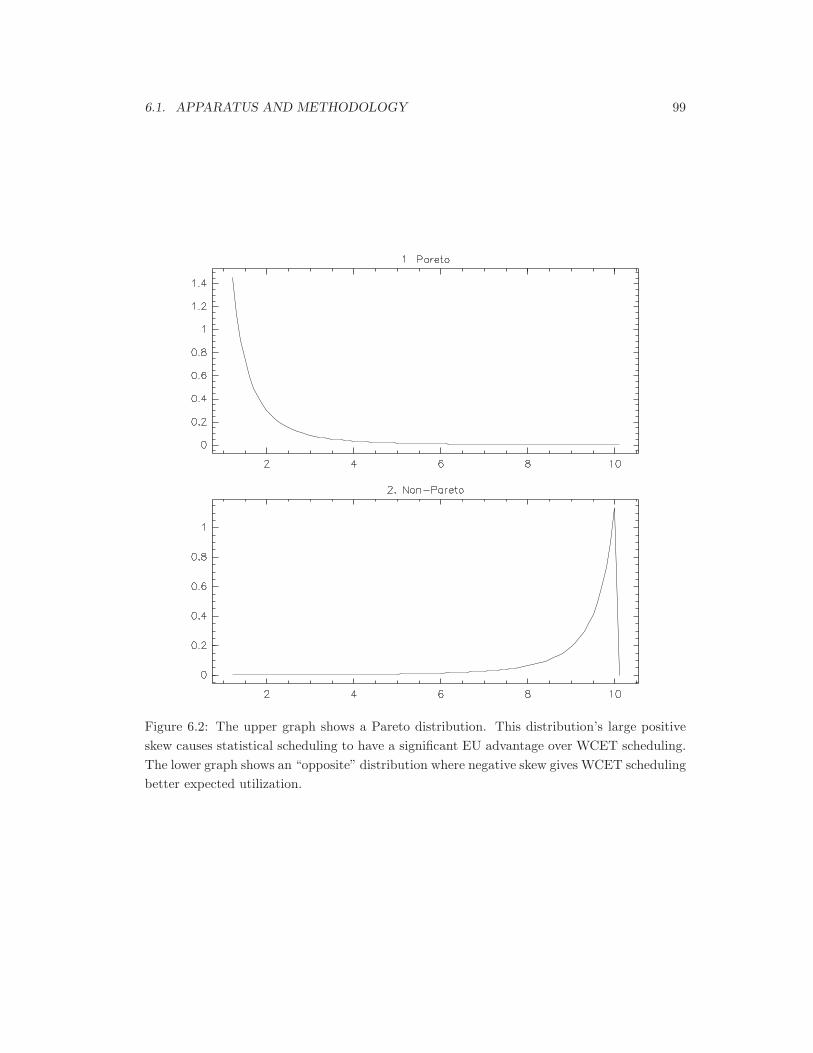
6.1. APPARATUS AND METHODOLOGY 99
Figure 6.2: The upper graph shows a Pareto distribution. This distribution’s large positiveskew causes statistical scheduling to have a significant EU advantage over WCET scheduling.The lower graph shows an “opposite” distribution where negative skew gives WCET schedulingbetter expected utilization.

100 CHAPTER 6. PERFORMANCE MEASUREMENTS
Figure 6.3: Running time distribution of the standard test performers at a 0.4 loading level.
Sinusoidal has a load loop identical to Jittered simple but executes for a+b sin(ci) iterationswhere i is the basic period, a is fixed, b is a scale factor and c adjusts the period. As withJittered simple, a composer task sets a, b and c. Besides having negative skew, Sinusoidal alsoprovides a worst case EU bound for liqui by having more than twice the standard deviationof Jittered.
Summarizing, the performance tests used four different synthetic performers. As shown inFigure 6.4, Simple, Synth and Jittered span the range of typical standard deviation to meanratios The histograms of the four synthetic test performers at the 0.4 loading level found inFigure 6.3 show how the distribution shapes of the synthetic test performers differ. Simple,Synth and Jittered have distributions similar to Figure 6.3(1). Conversely, Sinusoidal providesa lower bound on liqui’s expected utilization and advantage over WCET estimation because,as shown in Figures 6.4 and 6.3, it has both a much higher standard deviation to mean ratio
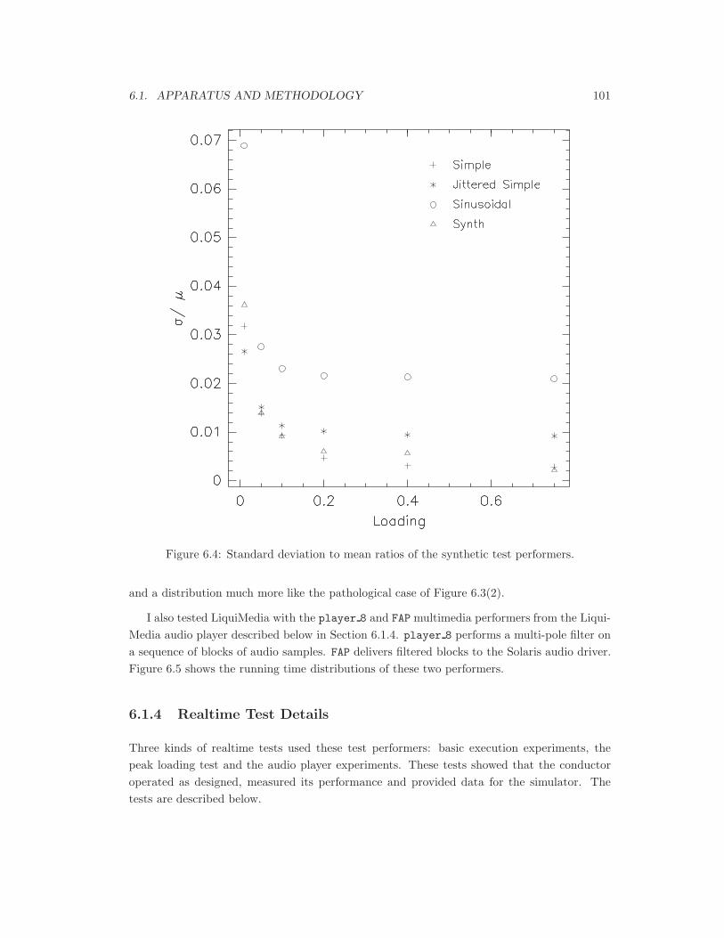
6.1. APPARATUS AND METHODOLOGY 101
Figure 6.4: Standard deviation to mean ratios of the synthetic test performers.
and a distribution much more like the pathological case of Figure 6.3(2).
I also tested LiquiMedia with the player 8 and FAP multimedia performers from the Liqui-Media audio player described below in Section 6.1.4. player 8 performs a multi-pole filter ona sequence of blocks of audio samples. FAP delivers filtered blocks to the Solaris audio driver.Figure 6.5 shows the running time distributions of these two performers.
6.1.4 Realtime Test Details
Three kinds of realtime tests used these test performers: basic execution experiments, thepeak loading test and the audio player experiments. These tests showed that the conductoroperated as designed, measured its performance and provided data for the simulator. Thetests are described below.

102 CHAPTER 6. PERFORMANCE MEASUREMENTS
Figure 6.5: Log histogram of the running times of the audio player performers.

6.1. APPARATUS AND METHODOLOGY 103
Basic Execution Tests
Basic execution tests consisted of running single instances of one of the four synthetic testperformers described in Section 6.1.3 at six different estimated loadings for one minute: 4561basic periods of the liqui prototype’s execution. The six different loadings were 0.01, 0.05,0.10, 0.20, 0.40 and 0.75 of the basic period.
Peak Loading Test
The peak-loading experiment provided the results needed to compute a performer’s runningtime overhead. Two versions exist: the performer-based peak-loading experiment and thethreaded peak-loading experiment.
In the performer-based experiment, a composer added blocks of 5 simple test performerswith a 0.01 loading to the schedule every 300 basic periods (approximately 4 seconds) until thelifetime admission control mechanism rejected the candidate schedule at an attempted load of95 performers.
That the scheduler rejected the candidate schedule at 95 shows the presence of its lifetimeadmission control mechanism. Figure 6.9 shows that the per-performer expected utilization isapproximately .9 when the schedule contains 90 instances of 0.01 simple. Consequently, thelifetime admission control mechanism rejected a candidate schedule containing 95 performersbecause this candidate has a Chebyshev-estimated running time of 1.06 of the basic period.The lifetime admission control mechanism reduced the schedule to 89 performers during aschedule re-verification when the size of schedule’s standard deviation caused the 90 performerschedule to be inadmissible.
The threaded peak-loading experiment provided the same data for a thread’s running timeoverhead. In the threaded peak-loading experiment, creative use of mutual exclusion primitivesforced a fine-grain interleaving of a fixed number of fixed-load threads. Each thread repeatedlyacquired the mutex, executed a synthetic load derived from the simple test performer andreleased the mutex. The software recorded the total execution time and the per-iterationthread running time.
Audio Player
The audio player experiment consisted of monitoring a stream of audio produced by an audioplayer application while the conductor recorded per-performer and total conductor runningtimes. The audio player was a Java application running inside a realtime Java virtual machine(JVM) built by LiquiMedia Inc. to run on top of the liqui prototype. Appendix D describesLiquiMedia Inc. and the realtime JVM in further detail.
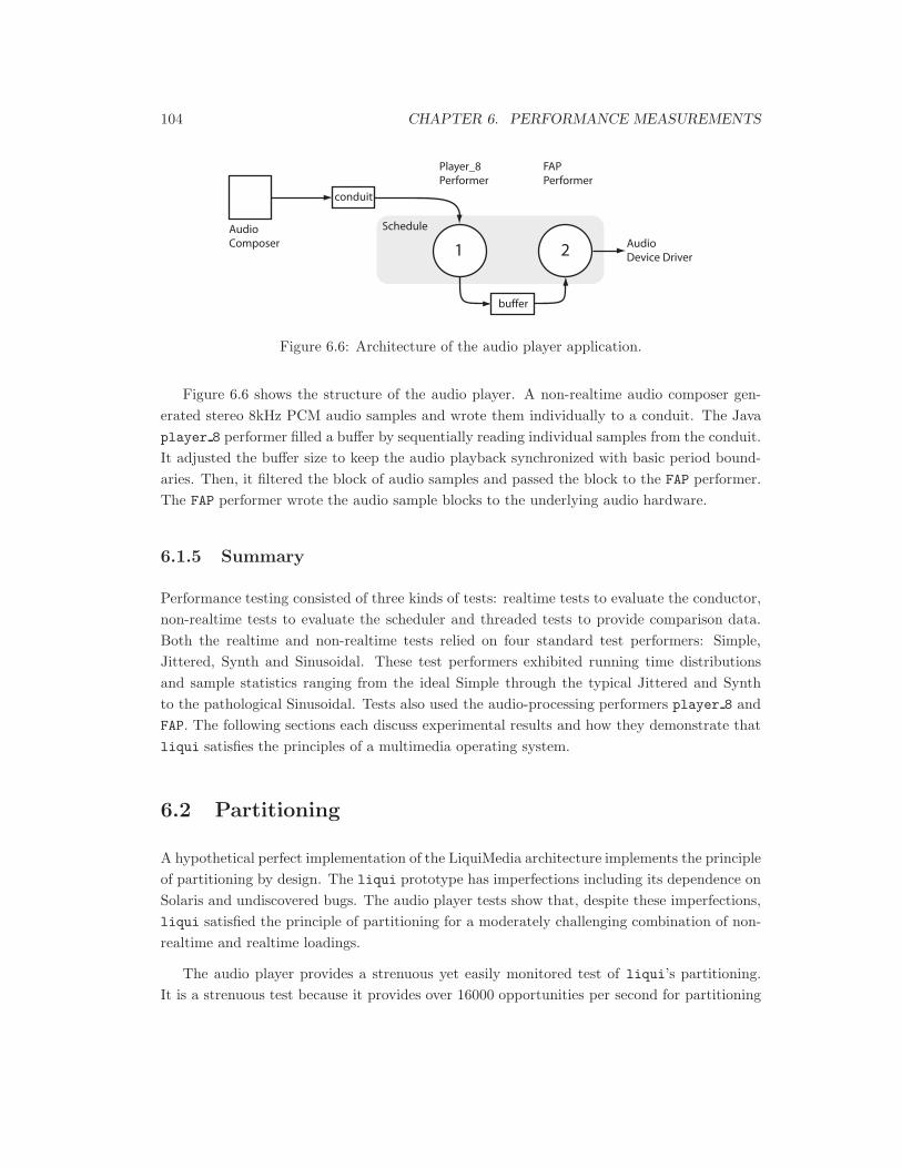
104 CHAPTER 6. PERFORMANCE MEASUREMENTS
buffer
conduit
AudioComposer Audio
Device Driver
Player_8Performer
Schedule
FAPPerformer
1 2
Figure 6.6: Architecture of the audio player application.
Figure 6.6 shows the structure of the audio player. A non-realtime audio composer gen-erated stereo 8kHz PCM audio samples and wrote them individually to a conduit. The Javaplayer 8 performer filled a buffer by sequentially reading individual samples from the conduit.It adjusted the buffer size to keep the audio playback synchronized with basic period bound-aries. Then, it filtered the block of audio samples and passed the block to the FAP performer.The FAP performer wrote the audio sample blocks to the underlying audio hardware.
6.1.5 Summary
Performance testing consisted of three kinds of tests: realtime tests to evaluate the conductor,non-realtime tests to evaluate the scheduler and threaded tests to provide comparison data.Both the realtime and non-realtime tests relied on four standard test performers: Simple,Jittered, Synth and Sinusoidal. These test performers exhibited running time distributionsand sample statistics ranging from the ideal Simple through the typical Jittered and Synthto the pathological Sinusoidal. Tests also used the audio-processing performers player 8 andFAP. The following sections each discuss experimental results and how they demonstrate thatliqui satisfies the principles of a multimedia operating system.
6.2 Partitioning
A hypothetical perfect implementation of the LiquiMedia architecture implements the principleof partitioning by design. The liqui prototype has imperfections including its dependence onSolaris and undiscovered bugs. The audio player tests show that, despite these imperfections,liqui satisfied the principle of partitioning for a moderately challenging combination of non-realtime and realtime loadings.
The audio player provides a strenuous yet easily monitored test of liqui’s partitioning.It is a strenuous test because it provides over 16000 opportunities per second for partitioning

6.3. SYNCHRONOUS REALTIME 105
failure. The conduit library is the only possible cause of partitioning failures because it is thesole gateway through liqui’s partition between realtime and non-realtime tasks. The audioplayer exercises the conduit library by passing stereo 8kHz audio through it sample-by-sample.This invocation pattern requires 16000 unique writes from a composer to the conduit whereone of the conduit library’s two failure cases can occur at every write.
The conduit library can fail in two ways: priority inversion or composer lock-out. I easilymonitored the audio player test by listening to its generated audio stream because each of thesefailure modes permanently disrupt the audio stream. Priority inversion halts the machine andso stops the audio playback. Composer lock-out repeatedly plays the same one second segmentof music. I could easily detect such a change while using the machine hosting liqui to editcode, handle e-mail and browse the web.
Twelve hours of error-free music playback on the liqui prototype showed that the conduitlibrary maintained partitioning in seven hundred million successive invocations. This result issufficient to confirm that liqui satisfies the principle of partitioning.
6.3 Synchronous Realtime
LiquiMedia’s architecture is both synchronous and realtime by design. Consequently, it sat-isfies the principle of synchronous realtime. However, as with all other realtime operatingsystems, LiquiMedia sacrifices utilization for realtime execution guarantees. This section dis-cusses the utilization levels achieved by liqui in the basic execution and audio player tests.
The measured expected utilization (EU) is compared to the expected utilization of RMSscheduling. Expected utilization can be compared in two ways: per-performer and over thewhole schedule. Per-performer compares liqui’s per-performer EU u(stat(p)) with the WCETestimator’s per-performer EU u(wcet(p)). The basic execution experiments show that Liqui-Media delivers per-performer expected utilization u(stat(p)) equal or better to the WCETestimator’s u(wcet(p)) at a firmness of 0.99 for typical σ/µ ratios and loadings.
In comparing expected utilizations over the whole schedule, liqui always has better ex-pected (and actual) utilization than RMS scheduling. An RMS operating system providesindependently authored tasks with a firmness of 1.0 but only when all tasks’ utilization doesnot exceed .693u(wcet(P)).1 liqui’s whole schedule expected utilization u(stat(P)) alwaysexceeds .693u(wcet(P)) because u(stat(p)) ≥ u(wcet(p)) implies u(stat(P)) ≥ u(wcet(P)) andsynchronous execution of tasks in LiquiMedia eliminates the .693 utilization cost of RMSscheduling.2
1Better RMS utilizations are possible when tasks have similar periods. However, an RMS operating system
supporting independently-authored tasks cannot rely on them having similar periods. Consequently, it is

106 CHAPTER 6. PERFORMANCE MEASUREMENTS
Figure 6.7: Expected utilization u(stat(p)) of the standard test performers at a firmness ofPc = 0.99. Variance caused by interrupts limit the expected utilization of smaller performers.As expected, the pathological sinusoidal performer has significantly poorer EU at all performersizes.
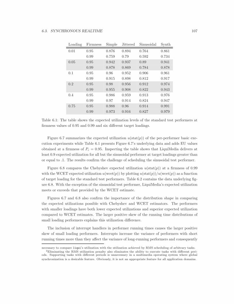
6.3. SYNCHRONOUS REALTIME 107
Loading Firmness Simple Jittered Sinusoidal Synth
0.01 0.95 0.876 0.894 0.764 0.8610.99 0.759 0.79 0.592 0.734
0.05 0.95 0.942 0.937 0.89 0.9410.99 0.878 0.869 0.784 0.878
0.1 0.95 0.96 0.952 0.906 0.9610.99 0.915 0.898 0.812 0.917
0.2 0.95 0.98 0.956 0.912 0.9740.99 0.955 0.908 0.822 0.943
0.4 0.95 0.986 0.959 0.913 0.9760.99 0.97 0.914 0.824 0.947
0.75 0.95 0.988 0.96 0.914 0.9910.99 0.973 0.916 0.827 0.979
Table 6.1: The table shows the expected utilization levels of the standard test performers atfirmness values of 0.95 and 0.99 and six different target loadings.
Figure 6.7 summarizes the expected utilization u(stat(p)) of the per-performer basic exe-cution experiments while Table 6.1 presents Figure 6.7’s underlying data and adds EU valuesobtained at a firmness of Pc = 0.95. Inspecting the table shows that LiquiMedia delivers atleast 0.9 expected utilization for all but the sinusoidal performer at target loadings greater thanor equal to .1. The results confirm the challenge of scheduling the sinusoidal test performer.
Figure 6.8 compares the Chebyshev expected utilization u(stat(p)) at a firmness of 0.99with the WCET expected utilization u(wcet(p)) by plotting u(stat(p))/u(wcet(p)) as a functionof target loading for the standard test performers. Table 6.2 contains the data underlying fig-ure 6.8. With the exception of the sinusoidal test performer, LiquiMedia’s expected utilizationmeets or exceeds that provided by the WCET estimate.
Figures 6.7 and 6.8 also confirm the importance of the distribution shape in comparingthe expected utilizations possible with Chebyshev and WCET estimators. The performerswith smaller loadings have both lower expected utilizations and superior expected utilizationcompared to WCET estimates. The larger positive skew of the running time distributions ofsmall loading performers explains this utilization difference.
The inclusion of interrupt handlers in performer running times causes the larger positiveskew of small loading performers. Interrupts increase the variance of performers with shortrunning times more than they affect the variance of long-running performers and consequently
necessary to compare liqui’s utilization with the utilization achieved by RMS scheduling of arbitrary tasks.2Eliminating the RMS utilization penalty also eliminates the ability to execute tasks with different peri-
ods. Supporting tasks with different periods is unnecessary in a multimedia operating system where global
synchronization is a desirable feature. Obviously, it is not an appropriate feature for all application domains.

108 CHAPTER 6. PERFORMANCE MEASUREMENTS
Figure 6.8: The graph compares u(stat(p)) with u(wcet(p)) for each of the standard testperformers at a range of performer sizes. Only statistically scheduled performers with a sinu-soidal running time distribution fail to meet or exceed the WCET bounds. Note the relativesuperiority of statistical scheduling for the highly variant smaller performers.
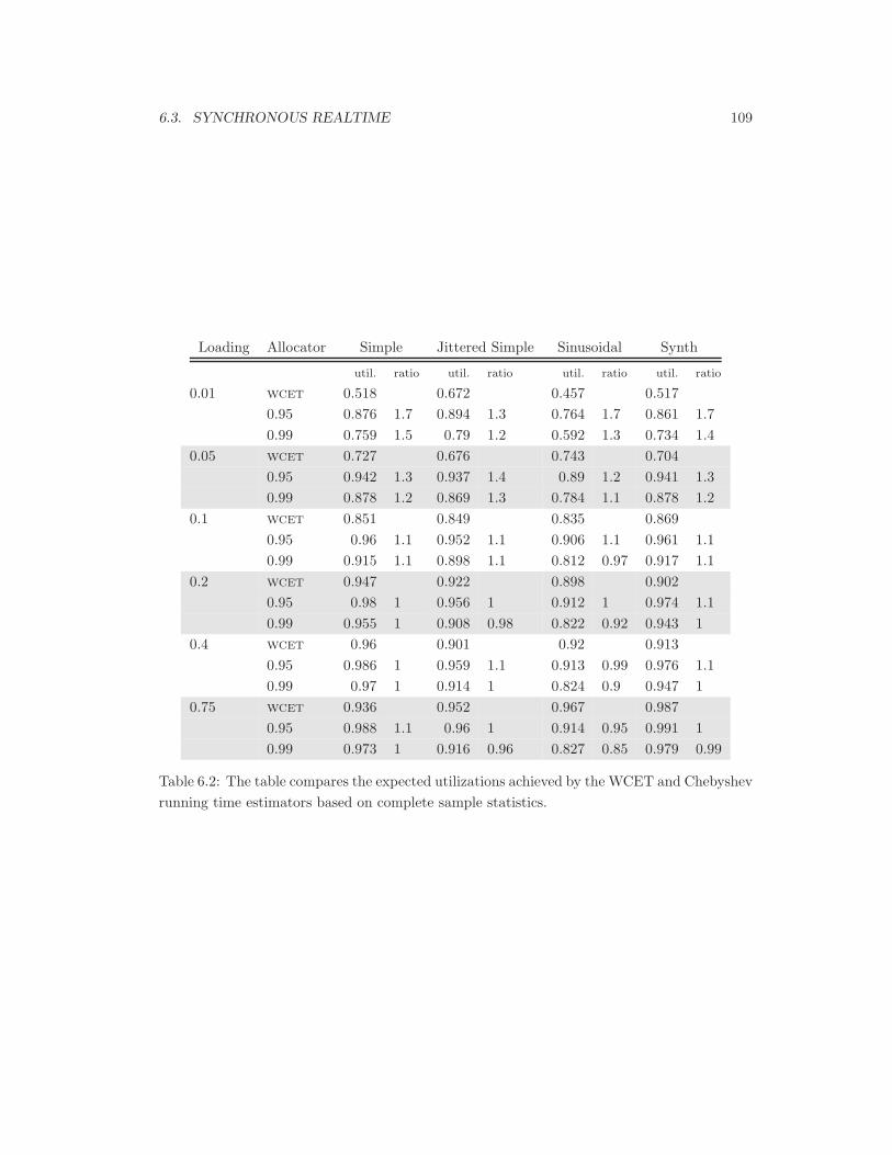
6.3. SYNCHRONOUS REALTIME 109
Loading Allocator Simple Jittered Simple Sinusoidal Synth
util. ratio util. ratio util. ratio util. ratio
0.01 wcet 0.518 0.672 0.457 0.5170.95 0.876 1.7 0.894 1.3 0.764 1.7 0.861 1.70.99 0.759 1.5 0.79 1.2 0.592 1.3 0.734 1.4
0.05 wcet 0.727 0.676 0.743 0.7040.95 0.942 1.3 0.937 1.4 0.89 1.2 0.941 1.30.99 0.878 1.2 0.869 1.3 0.784 1.1 0.878 1.2
0.1 wcet 0.851 0.849 0.835 0.8690.95 0.96 1.1 0.952 1.1 0.906 1.1 0.961 1.10.99 0.915 1.1 0.898 1.1 0.812 0.97 0.917 1.1
0.2 wcet 0.947 0.922 0.898 0.9020.95 0.98 1 0.956 1 0.912 1 0.974 1.10.99 0.955 1 0.908 0.98 0.822 0.92 0.943 1
0.4 wcet 0.96 0.901 0.92 0.9130.95 0.986 1 0.959 1.1 0.913 0.99 0.976 1.10.99 0.97 1 0.914 1 0.824 0.9 0.947 1
0.75 wcet 0.936 0.952 0.967 0.9870.95 0.988 1.1 0.96 1 0.914 0.95 0.991 10.99 0.973 1 0.916 0.96 0.827 0.85 0.979 0.99
Table 6.2: The table compares the expected utilizations achieved by the WCET and Chebyshevrunning time estimators based on complete sample statistics.

110 CHAPTER 6. PERFORMANCE MEASUREMENTS
push the running time distribution of a small loading performer toward the positive skewPareto distribution shown in Figure 6.2(1).3
The Simple performer in Figure 6.2 clearly shows the “noise floor” caused by interruptsbecause it executes a constant number of assembly language instructions in each invocation.Separately accounting for interrupts would remove their contribution to a performer’s vari-ance but is of dubious benefit because it does not correct for the variance added by cacheand TLB misses following an interrupt handler’s execution.4 Consequently, the additionalsystem complexity needed to separate interrupt running time from performer running time isboth pointless and unwarranted because liqui already delivers firmness levels sufficient formultimedia stream generation.
Because embedded interrupts make the PDFs of short-duration performers resemble thedistribution shown in Figure 6.2(1), the Chebyshev-style estimator delivers at least 25% greaterexpected utilization than the WCET estimator for synthetic test performers with loadings be-low 0.05. For test performers with higher-loadings, the Chebyshev-style estimator provides onlya 0.05% expected utilization advantage. While low, this level of expected utilization remainsacceptable because it permits liqui to execute independently-authored performers at a firm-ness of 0.99. However, if performers encountered in practice have running time distributionswith negative skew such as shown in Figure 6.2(2), then support for independently-authoredperformers may come at the cost of impractically low utilizations.
Fortunately, realistic signal-processing performers such as a MPEG decoder have positiveskew distributions similar to the Pareto PDF shown in Figure 6.2(1) [AB98b]. Also, as shown inFigure 6.5, the signal-processing performers FAP and player 8 from the audio player describedabove in Section 6.1.4 have positive skew distributions more like figure 6.2(1) than figure 6.2(2).
Table 6.3 shows u(stat(p)), u(wcet(p)) and u(stat(p))/u(wcet(p)) for the audio performersFAP and player 8. For player 8, the Chebyshev-style estimator’s expected utilization is 2.6times better than the WCET estimator’s EU while for FAP, the Chebyshev-style estimatorprovides an order of magnitude improvement in expected utilization. For such performers,the Chebyshev estimator offers significant expected utilization advantages over the WCETestimator.
3Recall that liqui is built on top of Solaris. In Solaris, interrupts come from sources such as the Ethernet
hardware and keyboard. Consider an operating regime where most interrupts are caused by the 2400 baud
keyboard interface. Here, interrupts occur with a probability of 1.6×10⁻⁵ per clock cycle and execute in about
.001 of a basic period. The number of interrupts is reasonably modeled by a binomial distribution.
A performer running for 0.01 of a basic period would expect to see .4 interrupts in its execution. As a result,
its most likely outcomes are either 0 or 1 interrupts. These two outcomes have a 10% difference in running time.
A performer running for .75 of a basic period expects 27.7 interrupts during its execution. Such a performer
would see only a a .1% difference in running times for invocations containing 27 or 28 interrupts.4An interrupt that flushes a performer from a processor cache significantly increases the running time of a
short-running performer. For example, each loop through simple takes 21ns on the LiquiMedia test machine
when executing from cache. However, reloading the code from main memory takes 500ns. If the processing of
interrupts flushes the cache for even 1% of Simple’s loop cycles, its execution time will rise by 23%.
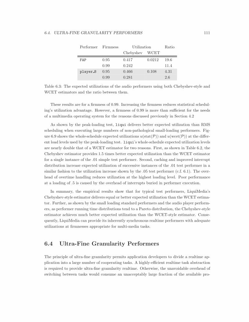
6.4. ULTRA-FINE GRANULARITY PERFORMERS 111
Performer Firmness Utilization RatioChebyshev WCET
FAP 0.95 0.417 0.0212 19.60.99 0.242 11.4
player 8 0.95 0.466 0.108 4.310.99 0.281 2.6
Table 6.3: The expected utilizations of the audio performers using both Chebyshev-style andWCET estimators and the ratio between them.
These results are for a firmness of 0.99. Increasing the firmness reduces statistical schedul-ing’s utilization advantage. However, a firmness of 0.99 is more than sufficient for the needsof a multimedia operating system for the reasons discussed previously in Section 4.2
As shown by the peak-loading test, liqui delivers better expected utilization than RMSscheduling when executing large numbers of non-pathological small-loading performers. Fig-ure 6.9 shows the whole-schedule expected utilizations u(stat(P)) and u(wcet(P)) at the differ-ent load levels used by the peak-loading test. liqui’s whole-schedule expected utilization levelsare nearly double that of a WCET estimator for two reasons. First, as shown in Table 6.2, theChebyshev estimator provides 1.5 times better expected utilization than the WCET estimatorfor a single instance of the .01 simple test performer. Second, caching and improved interruptdistribution increase expected utilization of successive instances of the .01 test performer in asimilar fashion to the utilization increase shown by the .05 test performer (c.f. 6.1). The over-head of overtime handling reduces utilization at the highest loading level. Poor performanceat a loading of .5 is caused by the overhead of interrupts buried in performer execution.
In summary, the empirical results show that for typical test performers, LiquiMedia’sChebyshev-style estimator delivers equal or better expected utilization than the WCET estima-tor. Further, as shown by the small loading standard performers and the audio player perform-ers, as performer running time distributions tend to a Pareto distribution, the Chebyshev-styleestimator achieves much better expected utilization than the WCET-style estimator. Conse-quently, LiquiMedia can provide its inherently synchronous realtime performers with adequateutilizations at firmnesses appropriate for multi-media tasks.
6.4 Ultra-Fine Granularity Performers
The principle of ultra-fine granularity permits application developers to divide a realtime ap-plication into a large number of cooperating tasks. A highly-efficient realtime task abstractionis required to provide ultra-fine granularity realtime. Otherwise, the unavoidable overhead ofswitching between tasks would consume an unacceptably large fraction of the available pro-

112 CHAPTER 6. PERFORMANCE MEASUREMENTS
Figure 6.9: The graph compares whole-schedule Chebyshev expected utilization u(stat(P))with WCET expected utilization u(wcet(P)) as a function of the number of performers in theschedule.

6.4. ULTRA-FINE GRANULARITY PERFORMERS 113
cessor resources. The experiments described in the remainder of this section compare liqui’sperformer-style task abstraction with the threaded task abstraction and show that performershave the efficiency levels needed to support the repeated execution of many thousands of tasks.
6.4.1 Conductor and Performer Overhead
Conductor overhead has fixed and marginal portions:
wp The per-performer overhead of the conductor.
wc The conductor’s fixed overhead independent of the number of performers executed.
These two constants satisfy the following equation:
ti −∑
p∈path(1,i)
tp,i = |path(1, i)|wp + wc (6.6)
where |path(1, i)| is the number of performers executed in basic period i, ti is the conduc-tor’s running time in basic period i including the time it spends executing performers and∑
p∈path(1,i) tp,i is the time spent executing performers.5
To reduce instrumentation overhead, the peak-loading experiment collected only the wholeconductor values ti for eight different loading levels ranging from 10 to 80 instances of the .01simple test performer. Substitute
min∀i
(tp,i)|path(1, i)| <∑
p∈path(1,i)
tp,i
for tp,i in Equation 6.6 to define an upper bound on wp. Then, an upper bound on liqui’sper-performer overhead wp is the slope of a linear regression fit of equation 6.7. Figure 6.10shows the regression.
ti −min∀i
(tp,i)|path(1, i)| > |path(1, i)|wp + wc (6.7)
The linear regression provides an upper bound on liqui’s per-performer overhead of wp of1566 nanoseconds.
6.4.2 Comparison
Comparing the 1556 nanosecond bound to the overhead of threads shows the efficiency advan-tages of the performer task abstraction. The threaded peak-loading experiment described inSection 6.1 measured the context switch time wf of Solaris user-space threads.
5Section B.4.1 defines the schedule structure and execution paths.
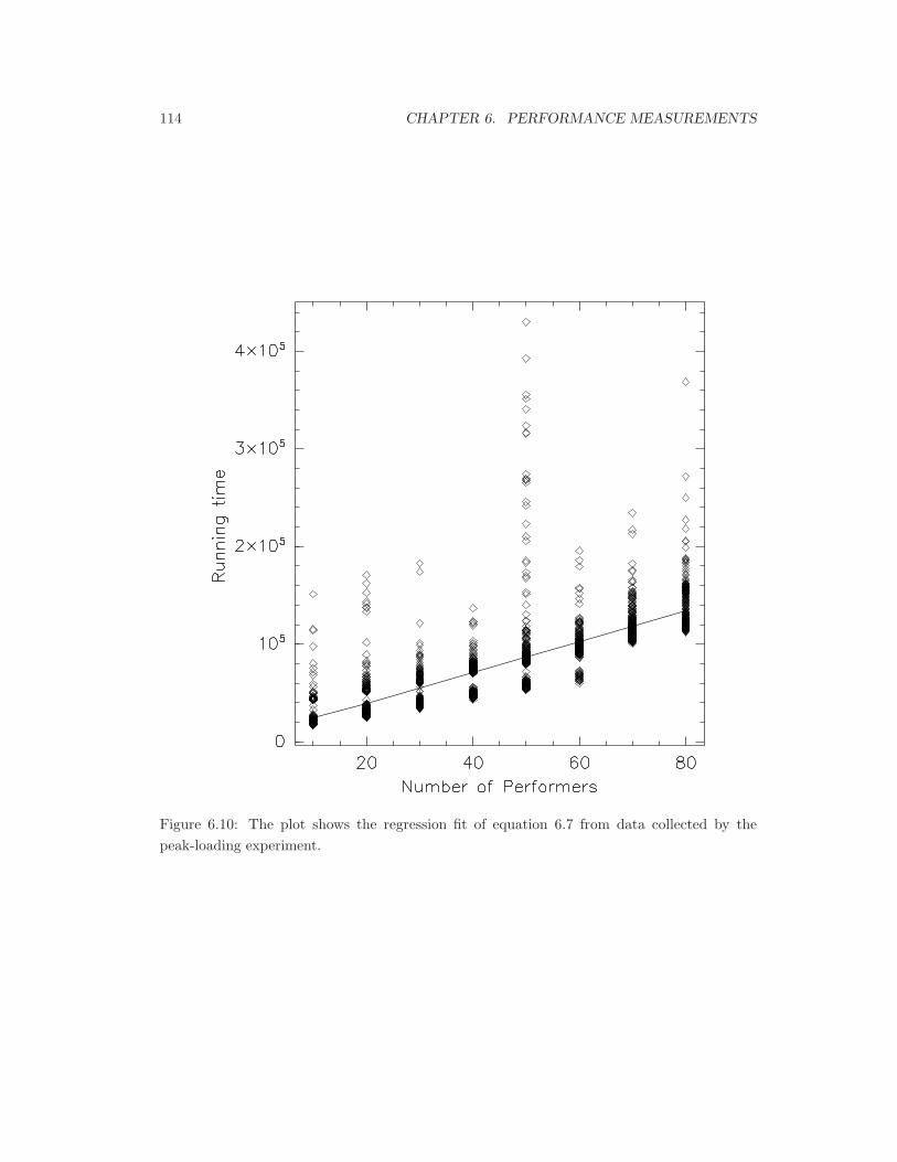
114 CHAPTER 6. PERFORMANCE MEASUREMENTS
Figure 6.10: The plot shows the regression fit of equation 6.7 from data collected by thepeak-loading experiment.

6.5. MODULARITY 115
Metric Threads Performers
overhead: wc .00118 0.00012Maximum number of tasks 886 8402
Table 6.4: The table compares LiquiMedia’s per-performer overhead (including the profilingand admission control mechanism) with the overhead of context switching between Solaristhreads. Performers are 9.48 times better.
Table 6.4 compares the normalized performer overhead wp and the thread overhead wf .It shows the per-task overhead as a fraction of the basic period and the maximum number oftasks possible. The maximum number of tasks in a basic period is bounded above by TB/wc
or TB/wf : the number of tasks at which the operating system overhead required to dispatchthem exceeds the length of the basic period.
The performer task abstraction supports 8402 tasks versus the threaded task abstraction’s886 tasks. Performers are 9.48 times more efficient than threads. However, the difference iseven more significant that the results in Table 6.4 suggest. First, the performer result is only alower bound on the maximum possible number of tasks. Second, LiquiMedia’s implementationhas abundant room for additional optimization whereas the thread results correspond to Sun’soptimized threads library.
For example, the conductor uses the Solaris gethrtime function twice for each performerinvocation. Converting the conductor to use the hardware performance counters lowers wp
by 1090 nanoseconds — taking the upper bound from 1566 to 476 nanoseconds. This im-provement increases LiquiMedia’s maximum number of tasks from 8402 to 27643 and givesthe performer task abstraction a 31 times advantage over the threaded task abstraction. Ad-ditional optimizations such as re-writing the conductor in assembly language would furtherimprove performance.
Finally, although interrupts contribute some portion of the per-performer overhead, thecomparison remains fair because the running of the threaded test also includes overhead causedby interrupts.
In summary, the results show that the performer task abstraction has a significantly loweroverhead than the thread-style task abstraction. This 9.48 times efficiency advantage overthreads shows that liqui satisfies the principle of ultra-fine grain realtime.
6.5 Modularity
LiquiMedia’s admission control mechanisms satisfy the principle of modularity. Three testresults support this claim. First, the sample mean and standard deviations collected by the
116 CHAPTER 6. PERFORMANCE MEASUREMENTS
conductor converge within the stream segregation threshold to sufficiently accurate approxi-mations of the underlying distribution’s mean and standard deviation. Second, given theseaccurate approximations, the instantaneous admission control mechanism eliminates all over-times for a large number of randomly-generated schedules. Third, the lifetime admissioncontrol mechanism only admits randomly-generated schedules with a firmness exceeding thedesired completion probability Pc.
6.5.1 Convergence
Successful operation of LiquiMedia’s lifetime and instantaneous admission control mechanismrequires that LiquiMedia’s approximation to the mean and standard deviation converge within1.5 seconds to values with better than probability Pc of approximating the true distributions’summary statistics. Further, admission testing within a stream’s segregation delay requiresmean values to converge within 150 milliseconds to the underlying distribution’s mean.
It is impossible to determine the true running time distribution φp(t) of a performer p.Instead, I will use the summary statistics for a population of 4000 performer executions (53seconds of the prototype’s execution) to provide an adequate approximation to the true dis-tribution’s moments.6 Given the number of samples, this is a reasonable assumption.7
Per-performer mean estimates converge rapidly to the entire sample mean. Figure 6.11 plotsthe normalized absolute value of the differences between LiquiMedia’s running approximationto the mean mp,i and the actual experimental summary statistic mp,4000. The difference isroughly bounded above by 1/2i so it takes at most 50 basic periods (0.7 seconds) for mp,i tolie within 1% of mp,4000. In fact, a significant proportion of mp,i for i > 100 lie within .1%of mp,4000. Moreover, means for all but .01 loading performers and Sinusoidal lie within 1%of mp,4000 in under 10 basic periods. This convergence rate supports statistical scheduling oftypical performers with a firmness of Pc = .99 within a user’s segregation threshold.
The graphs in Figure 6.11 also show two other interesting features. First, the graphshave large y-axis spiking as the number of included samples approaches 4000. The occasionalbasic periods in which the performer has an unusually long running time explain these spikes.Second, as expected, convergence rates are poorest for the performers (as shown in Figure 6.4)with the largest µ/σ ratios: Sinusoidal is worst at large loadings while all performers are poor
6The tests ran for 4561 basic periods – one minute. Truncating that data to 4000 samples improved the
appearance of the graphs.7Define Z to be
Z =mp,i − µp
σp/√
i.
Then, the central limit theorem holds that as i → ∞, the distribution of Z is the standardized normal
distribution n(z; 0, 1) [WM78]. I used this theorem to verify the assumption that 4561 samples of a performer’s
execution adequately approximate its true distribution. Given i = 4000 and conservatively assume that σp <
3sp,4000. Then, for the performer Jittered simple, mp,4000 − µp < .003mp,4000 with a probability of .999.
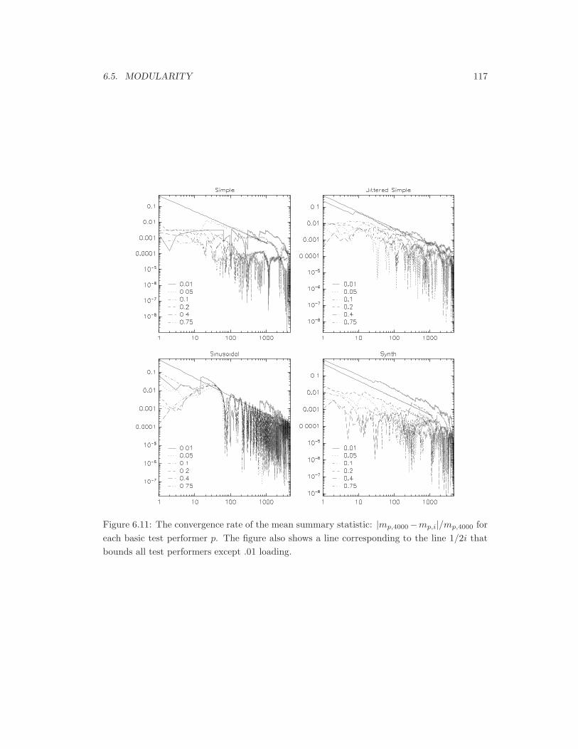
6.5. MODULARITY 117
Figure 6.11: The convergence rate of the mean summary statistic: |mp,4000−mp,i|/mp,4000 foreach basic test performer p. The figure also shows a line corresponding to the line 1/2i thatbounds all test performers except .01 loading.

118 CHAPTER 6. PERFORMANCE MEASUREMENTS
Figure 6.12: The convergence rate of the standard deviation summary statistic: |sp,4000 −sp,i|/mp,4000 for each test performer i. The figure also shows a line corresponding to the line1/i which bounds all test performers except .01 loading.
at the .01 loading level. Fortunately, inaccurate estimates have the smallest impact on lowloading performers.
Per-performer standard deviations also converge sufficiently rapidly for the needs of statis-tical scheduling. Figure 6.12 shows that, except for the .01 loading test performer, the errorin the collected standard deviation |sp,4000 − sp,i| is within .01 of mp,i in 10 basic periods andwithin .001 of mp,i in 100 basic periods. As a result, stat(p) is off by at most .1mp,10 after thesegregation delay and .01mp,100 after the expectation delay. This convergence rate is sufficientfor successful statistical scheduling.
As with Figure 6.11, the performers with the largest µ/σ ratios — particularly the .01 load-ing performer — have the poorest convergence rates in Figure 6.12. Consequently, performers
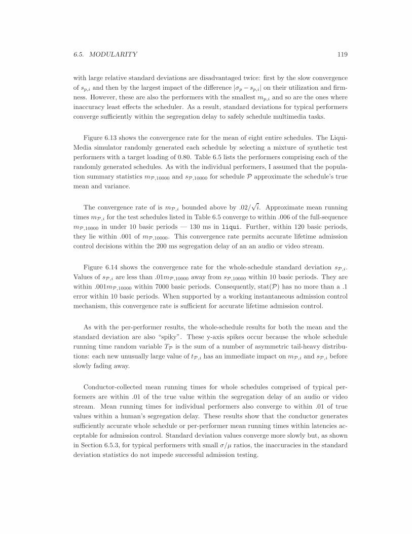
6.5. MODULARITY 119
with large relative standard deviations are disadvantaged twice: first by the slow convergenceof sp,i and then by the largest impact of the difference |σp− sp,i| on their utilization and firm-ness. However, these are also the performers with the smallest mp,i and so are the ones whereinaccuracy least effects the scheduler. As a result, standard deviations for typical performersconverge sufficiently within the segregation delay to safely schedule multimedia tasks.
Figure 6.13 shows the convergence rate for the mean of eight entire schedules. The Liqui-Media simulator randomly generated each schedule by selecting a mixture of synthetic testperformers with a target loading of 0.80. Table 6.5 lists the performers comprising each of therandomly generated schedules. As with the individual performers, I assumed that the popula-tion summary statistics mP,10000 and sP,10000 for schedule P approximate the schedule’s truemean and variance.
The convergence rate of is mP,i bounded above by .02/√
i. Approximate mean runningtimes mP,i for the test schedules listed in Table 6.5 converge to within .006 of the full-sequencemP,10000 in under 10 basic periods — 130 ms in liqui. Further, within 120 basic periods,they lie within .001 of mP,10000. This convergence rate permits accurate lifetime admissioncontrol decisions within the 200 ms segregation delay of an an audio or video stream.
Figure 6.14 shows the convergence rate for the whole-schedule standard deviation sP,i.Values of sP,i are less than .01mP,10000 away from sP,10000 within 10 basic periods. They arewithin .001mP,10000 within 7000 basic periods. Consequently, stat(P) has no more than a .1error within 10 basic periods. When supported by a working instantaneous admission controlmechanism, this convergence rate is sufficient for accurate lifetime admission control.
As with the per-performer results, the whole-schedule results for both the mean and thestandard deviation are also “spiky”. These y-axis spikes occur because the whole schedulerunning time random variable TP is the sum of a number of asymmetric tail-heavy distribu-tions: each new unusually large value of tP,i has an immediate impact on mP,i and sP,i beforeslowly fading away.
Conductor-collected mean running times for whole schedules comprised of typical per-formers are within .01 of the true value within the segregation delay of an audio or videostream. Mean running times for individual performers also converge to within .01 of truevalues within a human’s segregation delay. These results show that the conductor generatessufficiently accurate whole schedule or per-performer mean running times within latencies ac-ceptable for admission control. Standard deviation values converge more slowly but, as shownin Section 6.5.3, for typical performers with small σ/µ ratios, the inaccuracies in the standarddeviation statistics do not impede successful admission testing.
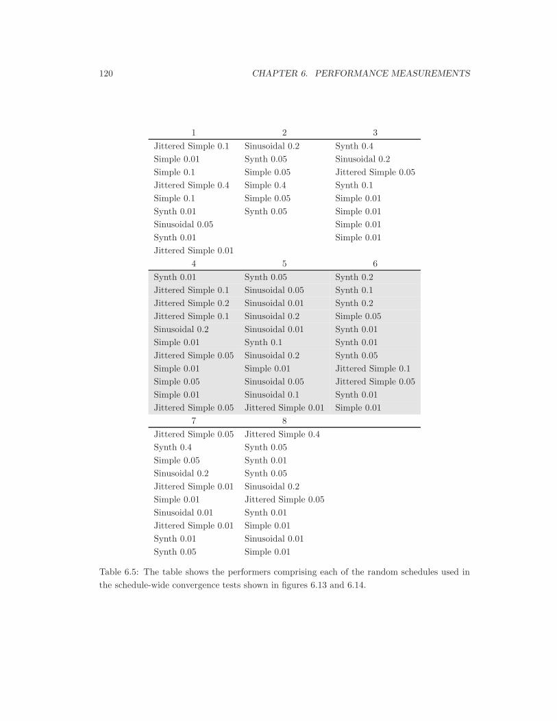
120 CHAPTER 6. PERFORMANCE MEASUREMENTS
1 2 3Jittered Simple 0.1 Sinusoidal 0.2 Synth 0.4Simple 0.01 Synth 0.05 Sinusoidal 0.2Simple 0.1 Simple 0.05 Jittered Simple 0.05Jittered Simple 0.4 Simple 0.4 Synth 0.1Simple 0.1 Simple 0.05 Simple 0.01Synth 0.01 Synth 0.05 Simple 0.01Sinusoidal 0.05 Simple 0.01Synth 0.01 Simple 0.01Jittered Simple 0.01
4 5 6Synth 0.01 Synth 0.05 Synth 0.2Jittered Simple 0.1 Sinusoidal 0.05 Synth 0.1Jittered Simple 0.2 Sinusoidal 0.01 Synth 0.2Jittered Simple 0.1 Sinusoidal 0.2 Simple 0.05Sinusoidal 0.2 Sinusoidal 0.01 Synth 0.01Simple 0.01 Synth 0.1 Synth 0.01Jittered Simple 0.05 Sinusoidal 0.2 Synth 0.05Simple 0.01 Simple 0.01 Jittered Simple 0.1Simple 0.05 Sinusoidal 0.05 Jittered Simple 0.05Simple 0.01 Sinusoidal 0.1 Synth 0.01Jittered Simple 0.05 Jittered Simple 0.01 Simple 0.01
7 8Jittered Simple 0.05 Jittered Simple 0.4Synth 0.4 Synth 0.05Simple 0.05 Synth 0.01Sinusoidal 0.2 Synth 0.05Jittered Simple 0.01 Sinusoidal 0.2Simple 0.01 Jittered Simple 0.05Sinusoidal 0.01 Synth 0.01Jittered Simple 0.01 Simple 0.01Synth 0.01 Sinusoidal 0.01Synth 0.05 Simple 0.01
Table 6.5: The table shows the performers comprising each of the random schedules used inthe schedule-wide convergence tests shown in figures 6.13 and 6.14.
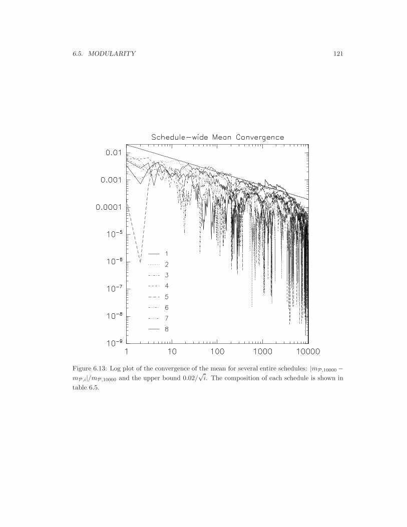
6.5. MODULARITY 121
Figure 6.13: Log plot of the convergence of the mean for several entire schedules: |mP,10000 −mP,i|/mP,10000 and the upper bound 0.02/
√i. The composition of each schedule is shown in
table 6.5.
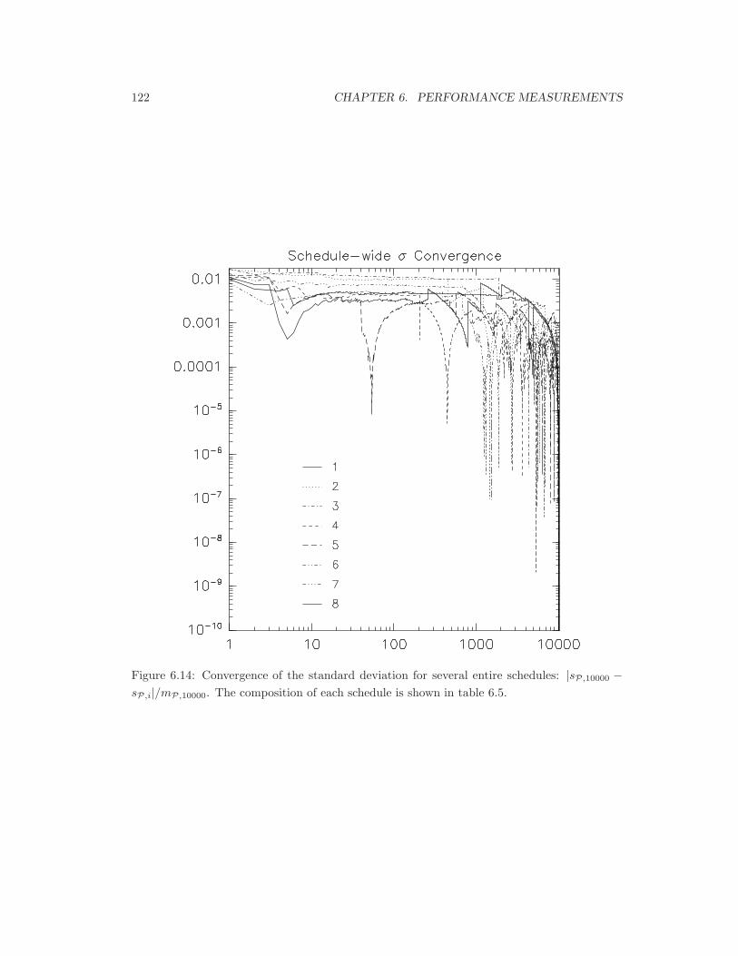
122 CHAPTER 6. PERFORMANCE MEASUREMENTS
Figure 6.14: Convergence of the standard deviation for several entire schedules: |sP,10000 −sP,i|/mP,10000. The composition of each schedule is shown in table 6.5.

6.5. MODULARITY 123
6.5.2 Instantaneous Admission Control
Once summary statistics are available, the conductor performs an instantaneous admissioncontrol test on each performer prior to executing it. It only executes a performer that has atleast probability Pc of executing completely before the end of the basic period. Otherwise, theconductor does not execute the performer and thereby causes it to experience a deferral.
When a performer attempts to execute past the end of the basic period, it experiences anovertime. The conductor suspends overtime performers and removes them from the schedulebecause LiquiMedia promises to execute performers atomically, The single basic period delayof a deferral is preferable to the possibly many basic periods needed for an application tore-schedule a suspended performer. LiquiMedia’s instantaneous admission control mechanismcompletely eliminates overtimes for a randomly chosen mixture of test performers.
Figure 6.15 compares the fraction of performer executions resulting in overtimes over arange of schedule loading levels with and without the instantaneous admission control mecha-nism. The graph shows overtime rates from 100 randomly generated schedules, each of whichexecuted in the LiquiMedia simulator for 10000 basic periods.
Figure 6.15 shows that liqui’s instantaneous admission control completely eliminates per-former overtimes on a randomly-chosen mixture of standard test performers.
6.5.3 Lifetime Admission Control
LiquiMedia’s scheduler also has a lifetime admission control mechanism. This mechanismverifies that every path through a candidate schedule has at least Pc of executing successfully.Provided with accurate summary statistics, this mechanism admission tests each path in theschedule using the algorithm presented in Section B.4.5.
The lifetime admission control mechanism operates correctly. Figure 6.16 shows that itcorrectly rejects every inadmissible schedule from a set of 1662 randomly generated schedules.
The graph is the result of the following experimental procedure. The simulator created1662 schedules comprised of a random selection of standard test performers. Each schedulecontained not less than 400 basic periods of execution. Each schedule’s observed Pc wascomputed by taking the ratio of the number of basic periods in which no overtimes took placeover the total number of executed basic periods.
The simulator applied the lifetime admission control test to each of the randomly generatedschedules. The lifetime admission control mechanism had a minimum firmness target of 0.9and performed the admission test using summary statistics from basic period i = 100. Therandomly generated schedules were binned into a histogram by their observed Pc value. Fig-ure 6.16 shows the proportion of the schedules in each bin that passed the lifetime admission

124 CHAPTER 6. PERFORMANCE MEASUREMENTS
Figure 6.15: The graph compares the normalized number of overtimes as a function of adesired schedule loading level with the instantaneous admission control mechanism (triangles)and without it (“x”). Instantaneous admission control completely eliminates overtimes.
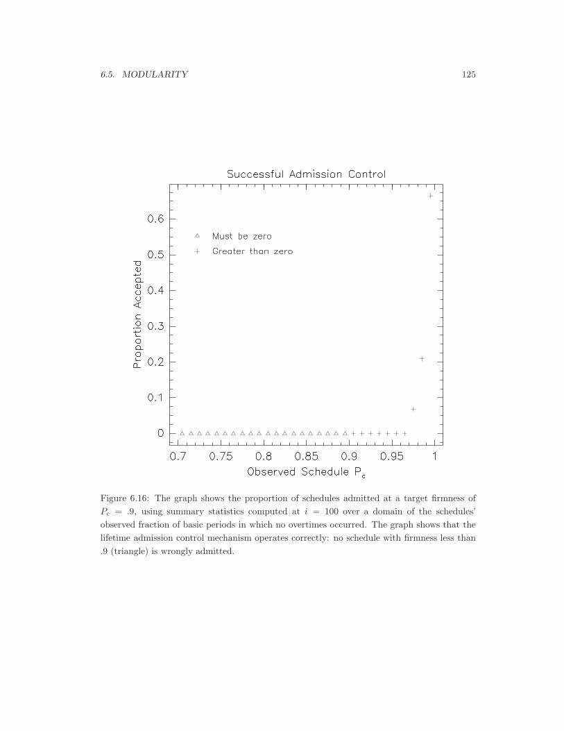
6.5. MODULARITY 125
Figure 6.16: The graph shows the proportion of schedules admitted at a target firmness ofPc = .9, using summary statistics computed at i = 100 over a domain of the schedules’observed fraction of basic periods in which no overtimes occurred. The graph shows that thelifetime admission control mechanism operates correctly: no schedule with firmness less than.9 (triangle) is wrongly admitted.

126 CHAPTER 6. PERFORMANCE MEASUREMENTS
control test. The figure shows that the admission test operates correctly as it does not wronglyadmit any schedules (plotted with triangles) whose observed firmness is less than .9.
Figure 6.16 also suggests that LiquiMedia’s admission control mechanism might be pes-simistic. While every admitted schedule has at least 0.9 probability of executing withoutovertimes, some of the rejected schedules may have more than 0.9 probability of executingsuccessfully.
Experimental limitations explain some of the observed pessimism. The success or failureof a schedule in each basic period is an independent binary random variable. The domain ofFigure 6.16 is the proportion of basic periods in which a schedule actually executed successfully.This number is normally distributed around the schedule’s actual but unknown probability ofsuccess. Highly variable schedules simulated for only a short number of basic periods canexecute successfully in every basic period but still have a finite probability of failure.
The admission control mechanism’s over-estimate of the schedule’s standard deviation atbasic period 100 explains the remainder of the pessimistic rejections. The Chebyshev-styleestimator computes a pessimistic bound for a schedule P when sP,100 considerably exceedsσP . The admission control mechanism incorrectly rejects some schedules on the basis of thispessimistic bound.
LiquiMedia’s feedback mechanism significantly reduces the impact of this pessimism inpractice. In normal operation, the scheduler adds only a single new application to an existingschedule comprised of established applications. The performers comprising the establishedapplications typically have summary statistics spanning many thousands of basic periods andso, as shown in Figure 6.14, have accurate summary statistics. This majority offsets the inac-curate standard deviations of performers newly added to the candidate schedule and enablesthe scheduler to admit a wider range of highly loaded schedules.
This section’s results demonstrate that LiquiMedia’s lifetime admission control mechanismalways detects a schedule with less than firmness Pc. Consequently, this mechanism providesthe decision functionality needed to satisfy the principle of modularity.
6.5.4 Feedback and Schedule Convergence
Satisfying the principle of modularity requires that LiquiMedia support the execution ofindependently-authored performers. Doing so has three architectural requirements. First, asshown in Section 6.5.1, LiquiMedia can measure the running time of independently-authoredperformers and schedules. Second, as shown in Sections 6.5.2 and 6.5.3, LiquiMedia mustbe able to use these measurements to decide if individual performers or whole schedules areadmissible. Finally, LiquiMedia must be able to correct a schedule that was previously correctbut is no longer so.
6.5. MODULARITY 127
LiquiMedia’s schedule feedback mechanism satisfies this final requirement of the principleof modularity by design. LiquiMedia’s feedback mechanism consists of the conductor providingupdated statistical summary information to the scheduler. The scheduler then verifies thatthe current schedule still has at least Pc of completing in a single basic period.
So long as accurate per-performer and schedule-wide statistical summary information isavailable and the admission control test operates as designed, the scheduler can always suc-cessfully convert an incorrect schedule into a correct schedule. LiquiMedia corrects an incorrectschedule by removing performers from it in order of increasing importance until the schedule iscorrect. Because the feedback is negative, the schedule is guaranteed to converge to a correctschedule.
As discussed above in Section 6.5.3, the conductor will gather accurate summary statisticsfor performers within 50 basic periods and accurate means for whole schedules within 10 basicperiods. The scheduler re-verifies the current schedule after 10, 35, 105, 4561 and then every9123 basic periods thereafter. These values correspond approximately to .1, .5, 1.5, 60 and120 seconds.
Three criteria guided the selection of these times: the perceptual thresholds discussed inSection 1.1, the convergence times of the summary statistics discussed in Section 6.5.1 andthe need to prevent numerical overflow in conductor-collected integer statistics as discussed inSection B.3.6.
Schedule verifications after 10 basic periods eliminate inadmissible performers prior tothe 200 ms segregation delay of a human’s auditory or visual modality. The verificationat .5 seconds improves the per-performer standard deviations available to the instantaneousadmission control mechanism. The verification at 1.5 seconds tests the schedule before ahuman’s expectation threshold and after the availability of more accurate per-performer andwhole-schedule statistics. The test at one minute verifies the schedule once accurate standarddeviations are available. Finally, re-verifications every two minutes keep accumulated sum-of-squares values from overflowing.
The chosen reverification times also provide sufficient time for the scheduler’s latency.For schedules with under ten performers and realtime loadings less than .75, the schedulercan verify a schedule between successive conductor invocations. When the schedule containsupward of a 100 performers, scheduler latency is under 8 basic periods from scheduling requestto posting.8
The performers responsible for the generation of well-established realtime streams maychange their behaviour. Perhaps through a coding error, data alteration or deliberate attackon the system, a mature performer may suddenly start to execute for a considerably longer ormore variable amount of time than the execution profile on whose basis it was admitted intothe schedule.
8Schedule life cycle is explained in Section B.4.6.
128 CHAPTER 6. PERFORMANCE MEASUREMENTS
The scheduler successfully handles this “embedded leak” situation by design. Unfortu-nately, the scheduler’s negative feedback heuristic cannot handle this situation without dis-rupting the operation of other possibly established streams. The scheduler always tries tocorrect a schedule by removing the least important scheduled performers. If an embedded leakis merely symptomatic of a performer requiring additional processor resources to respond touser requests, then the negative feedback mechanism will correct the situation within a minuteor, if the embedded leak has caused an overtime, within 1 to 8 basic periods.
Unfortunately, the negative feedback mechanism’s response suspends many correct per-formers when an important performer causes the embedded leak deliberately or through pro-grammer error. However, it is not possible to automatically determine if a performer’s use ofadditional processor resource constitutes a programming defect or a genuine need.
6.6 Summary
This chapter has presented a number of performance tests on the liqui prototype and simula-tor whose results confirm that LiquiMedia’s design satisfies the four principles of a multimediaoperating system. The tests measure the limitations in the liqui prototype and show that itoperates successfully as designed on a range of typical performers. In particular, the chapterhas shown the following.
• The audio player tests show that liqui satisfies the principle of partitioning.
• liqui implements the principle of synchronous realtime by design. Its use of the Cheby-shev estimator delivers equal or better expected utilization than the WCET estimatorfor non-pathological test performers and vastly superior expected utilization levels forrealistic audio-processing performers.
• liqui satisfies the principle of ultra-fine granularity because its performer implementa-tion is 9.48 times more efficient than the thread task abstraction on the same machine.
• liqui can measure, admission test and correct schedules comprised of arbitrary mixturesof typical performers within a human user’s 200 ms segregation threshold and obtainaccurate per-performer summary statistics within a human user’s 1.5 second expectationthreshold. This capability satisfies the principle of modularity.
Chapter 7
Future Work
LiquiMedia has been a large project. Consequently, this thesis defers many interesting areasof investigation. This chapter describes some of these areas. It begins with improvements tothe LiquiMedia implementation and experiments. Then the chapter presents more conceptualextensions to the research and finally product versions of the LiquiMedia architecture. Withineach category, possible future work is presented in order of increasing ambition.
7.1 Experimentation and Analysis
Chapter 6 describes an empirical validation of LiquiMedia’s operation on a range of typicalcases. This section discusses experiments that widen the scope of the empirical validation andexplore more of the prototype’s performance envelope.
7.1.1 Scheduler Operation
LiquiMedia’s scheduler does not operates realtime. This design aspect reduces overhead in-side the realtime code path and therefore helps LiquiMedia satisfy the principle of ultra-finegranularity. However, because it does not operate in real-time, no experiments evaluated thescheduler’s throughput and running time.
The scheduler’s running time overhead is proportional to the number of schedule pathsand performers. LiquiMedia cannot support schedules that take longer to admission testthan the time available between the most frequent schedule re-verifications. Consequently, thescheduler’s overhead bounds the maximum possible number of performers. Future research willinclude deriving theoretical limits on the time needed to verify a schedule and the maximumnumber of performers supported at any given re-verification interval.
129
130 CHAPTER 7. FUTURE WORK
This theoretical derivation also requires corresponding experiments. It is important tomeasure the following:
(i) the time needed to update the summary statistics as a function of the number of per-formers,
(ii) the time needed to admit a schedule as a function of the number of performers and pathsthrough the schedule graph, and
(iii) the average latency of a schedule re-verification from the moment when the conductorrequests one until the scheduler posts the new re-verified schedule.
These results determine the processor reserve needed to guarantee adequate schedule veri-fication rates. The following approaches can lower this overhead if it proves excessive.
(i) Reduce the cost of schedule verification by caching path fragments from previous verifi-cation attempts.
(ii) Modify the conductor to perform usage-tracking on schedule paths and to re-verify onlythose paths for which performers have generated new statistical summary information.
(iii) Explore the impact of reducing the schedule verification rate.
7.1.2 Feedback Tests
The scheduler’s negative feedback mechanism is guaranteed to reduce an incorrect schedule toa correct schedule. However, the existing results do not include a measure of how long it takesthe scheduler to remove incorrect performers from the schedule. Consequently, it is importantto add simulation of schedule feedback to the LiquiMedia simulator. Subsequent research willthen explore the operation of the scheduler as it handles incorrect performers and measure theconvergence rate from an incorrect to a correct schedule.
The envisaged experiment performs admission control tests with both the simulator andliqui on randomly generated schedules at a variety of schedule ages and records the evolu-tion of the schedules. The incorrect schedule consists of a mixture of correct and incorrectperformers where incorrect test performers are constructed from the existing test performersusing the three following techniques.
Enlarge Enlarge the mean running time of one of the performers described in Section 6.1.3 sothat its estimated running time exceeds the available time.
Vary Increase the variance of an instance of Sinusoid or Jittered so that its mean runningtime is less than the available running time but its estimated running time stat(p)exceeds the available time.

7.1. EXPERIMENTATION AND ANALYSIS 131
Grow After some configurable number of basic periods, grow the performer’s mean or vari-ance until its estimated running time can no longer be accommodated. The slopeof the increase is configurable at the time of performer creation and includes theimportant special case of a step function.
The results include the number of basic periods that liqui spends on the schedule life cycle,the average depth of the verification request conduit and the correlation between scheduleverification rates and the operation of the instantaneous admission control mechanism.
7.1.3 Varied Loadings
The LiquiMedia simulator uses only statistical profile data generated by the liqui prototypewith the typical test performers described in Section 6.1.3. However, future development willinclude extending the simulator to synthesize statistical profile data corresponding to bothrealistic multimedia loads and performers with extreme σ/µ ratios. The following runningtime distributions will be implemented:
(i) the Pareto distribution shown in Figure 6.2(1),
(ii) the “negative” Pareto shown in Figure 6.2(2),
(iii) per-frame MPEG decompression timings, and
(iv) frame-drawing timings in an interactive video game such as Quake.
The experiments on the scheduler described in Chapter 6 can then be repeated withthese additional performer types. In particular, this work will further demonstrate that theChebyshev-style estimator maintains its utilization advantages over the WCET estimator fora more diverse selection of performer loadings.
7.1.4 Expanding the Envelope
The simulations and experiments described in Chapter 6 do not fully explore LiquiMedia’s per-formance envelope. Many interesting issues remain. Future research will exercise LiquiMediaover a wider range of firmness and loadings.
High load experiments have LiquiMedia running with an average load in excess of an entirebasic period. By deactivating the lifetime admission control mechanism, a modification of thepeak loading test can force conductor loads that exceed 1.0. Thanks to the instantaneousadmission control mechanism, such a configuration should retain the configured performer
132 CHAPTER 7. FUTURE WORK
firmness while possibly delivering increased utilization levels. It will also further validate theoperation of instantaneous admission control mechanism.
Second, additional research will include conducting experiments over a wider range ofperformer firmness values. The existing results are only for firmness Pc = .99 and .95. Thesevalues are appropriate for multimedia stream generation applications. However, tests at moreconservative and more aggressive settings will evaluate LiquiMedia’s suitability outside ofmultimedia stream generation applications.
7.1.5 Comparisons
This thesis has only compared LiquiMedia to RMS scheduling. The results confirm that underconditions appropriate for multimedia applications, statistical scheduling provides, at the costof hard realtime guarantees, superior whole-schedule processor utilization compared to RMS.The literature contains a wide variety of other scheduling techniques that also sacrifice hardrealtime guarantees to improve processor utilization. The results of future research shouldcompare LiquiMedia’s utilization, performance and handling of untrustworthy performers tooperating systems that use rate-based scheduling such as SMART and BERT [Nie99, BPM99].
7.1.6 Time Series Analysis
The conductor collects per-performer and per-schedule statistical profile data. This informa-tion is a time-series. There is an extensive mathematical literature concerning time-seriesanalysis [FBL+03]. Incorporating results from this literature into LiquiMedia could improvethe accuracy of the scheduler.
7.2 Prototype Enhancements
I bounded liqui’s development time by deferring a variety of interesting but non-essentialfeatures. Completing some of these features can significantly increase liqui’s performance.Others are natural generalizations that warrant investigation. This section describes suchextensions to the prototype.
7.2.1 Reducing Overhead
Two implementation optimizations will further reduce liqui’s already low per-performer over-head. First, the LiquiMedia prototype’s handling of saved stack frames for trapping per-performer exceptions should be rewritten in assembly language. The existing implementation

7.2. PROTOTYPE ENHANCEMENTS 133
uses setjmp. This call saves more state than necessary. An assembly language implementa-tion would save the minimum amount of processor state. Second, the conductor’s computationof summary statistics also needs to be re-written in assembly language. In particular, a by-hand implementation of the computation of s2
p,i and mp,i should take less than ten assemblyinstructions.
7.2.2 Timing
Conversion of the prototype to use hardware timing promises to have an even greater impacton LiquiMedia’s per-performer overhead. The prototype used the gethrtime function call toobtain monotonically increasing high-precision time values. Figure 1 shows that liqui invokesthis routine at least twice for every performer executed by the conductor. Both the accuracyof the timing information returned by this routine and the overhead of the conductor itself arelimited by the running time of the gethrtime function.
As discussed in Section 6.4.2, the gethrtime function call takes approximately 545ns tocomplete. Future work will therefore include replacing the calls to the gethrtime functionwith an assembly language macro that provides equivalent functionality via the cycle-countingfacilities in the UltraSparc processor.1
Switching the liqui prototype to hardware-assisted timing should reduce the per-performeroverhead of the conductor by at least 70%. Repeating the peak-loading test described inSection 6.1.4 will measure the extent of the improvement.
7.2.3 Enhanced Conduits
While not a direct contributor to per-performer overhead, the implementation of liqui’sconduit library can also be improved. The current conduit implementation uses the Solariskernel’s mutual exclusion primitives and therefore exposes conduit-using performers to kernelcall and kernel scheduling overhead.
A more efficient implementation should be possible. Conduit primitives can use the atomicswap assembly language instructions found on recent Sparc and IA32 hardware [Int99, SPA93].A careful combination of atomic swap instructions with a well-designed spin-lock permitsimplementing the conduit read and write operations in fewer than ten assembly languageinstructions.
1Processors such as the UltraSparc and IA32 have efficient hardware cycle counting facilities [Int99, SPA93].
134 CHAPTER 7. FUTURE WORK
7.2.4 Per-Performer Firmness
LiquiMedia provides a flexible trade-off between utilization and firmness. The liqui proto-type does so globally with the Pc parameter. As a result, every performer shares the samefirmness/utilization trade-off. This restriction is arbitrary and can be eliminated. A futureversion of liqui will provide per-performer firmness settings.
The LiquiMedia prototype provides a mechanism for adjusting an application’s importance.Per-performer firmness will be integrated into this mechanism so it permits independent ad-justment of firmness and importance.2
How to use independent firmness and importance remains a subject of future research. Oneparticularly interesting open issue is the user interface for a graphical tool that permits theuser to adjust the relative importance and firmness of applications in a way that maximizesuser satisfaction. The programmatic API for adjusting both firmness and importance will alsorequire investigation.
7.2.5 Instrumentation
Lastly, the liqui prototype can benefit from improved instrumentation. Modifying the con-ductor to record complete whole-schedule statistical summary data including the path takenthrough the schedule graph will provide additional valuable experimental data. Also, thescheduler will record the running time of schedule verifications. An extended instrumentationlibrary will integrate this new data with the existing facilities for recording per-performer andper-schedule running time information.
Several miscellaneous improvements are also desirable. The liqui prototype will labeldata sets in a standardized way and insure that each dataset includes a representation of theschedule graph. The liqui prototype should also successfully preserve as much accumulateddata as possible in the advent of a crash.
These enhanced data recording facilities lay the foundation for a general persistence mech-anism in LiquiMedia. Accumulated statistics will be preserved between executions to permitrestarting performers with previously accumulated summary statistics.
7.2.6 Processor Redistribution
LiquiMedia preserves established applications at the expense of new applications. This is adesirable default behaviour. For example, starting a new application should never jeopardize
2This independence has practical limitations. Some combinations of firmness and importance significantly
increase the likelihood that a performer will not be scheduled.
7.3. MULTIPROCESSOR SUPPORT 135
the operation of an existing source of a multimedia stream. However, its rigidity can also be aweakness. For example, the user might wish to reduce the processor consumed by a video playerso that a video conference can deliver a higher quality of service. Consequently, LiquiMedianeeds a mechanism that permits applications to contend for recently freed processor resources.
The liqui prototype has a partial implementation of such a mechanism. The implementa-tion of the processor redistribution mechanism should be completed and tested to insure thatthe scheduler’s feedback mechanism remains stable while applications contend for availableprocessor resources.
The user interface to this API also requires research. A UI for the processor redistribu-tion mechanism must clearly show that the amount of processor is finite and increasing oneapplication’s allocation is always at the expense of the other applications.
7.3 Multiprocessor Support
At present, liqui permits only a single conductor. While non-realtime threads can freelyexecute on the remaining processors, this arrangement does not take maximum advantage ofmultiprocessors. However, the existing structure does handle the important special case of ageneral purpose processor scheduling performers for a single conductor running on a separatepurpose-built multimedia processor.
7.3.1 Multiple Conductors
A more general arrangement permits one conductor instance for each general purpose processorin a symmetric multiprocessor machine. Successfully implementing such an extension whilestill satisfying the principle of modularity requires additional research in two areas.
First, the existing conduit mechanism permits performers to access conduits cheaply be-cause the conductor maintains a global lock on conduit access. Two conductors cannot suc-cessfully execute at the same time if they must contend for the same global conduit lock. Amultiprocessing LiquiMedia implementation requires a conduit implementation that permitstwo different conductors to finely interleave access to a single conduit. Resolving this issue isprimarily an implementation challenge.
Second, conduits provide no mechanism for a single application to synchronize the exe-cution of performers running on different processors except at basic period boundaries. Theresultant latencies for inter-performer communication are impractical. Further, the principleof synchronous realtime permits developers to assume that no two performers ever executesimultaneously. Performers executing in separate conductors violate this assumption.
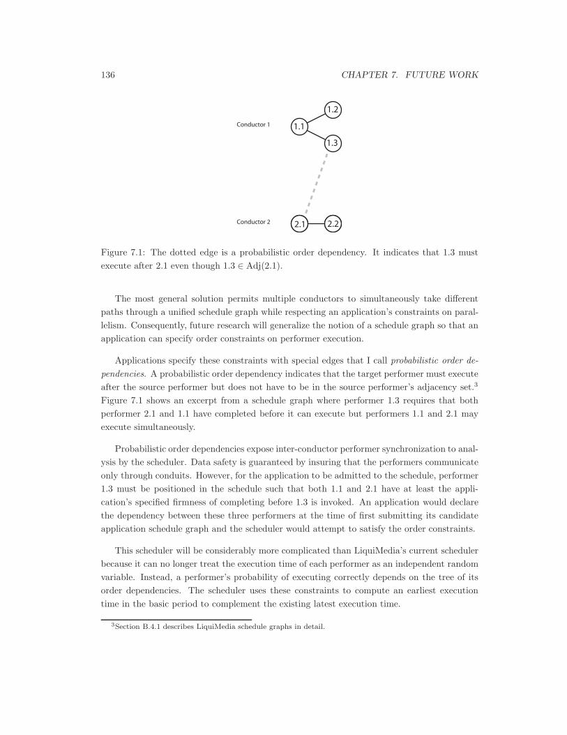
136 CHAPTER 7. FUTURE WORK
1.1
1.2
1.3
2.2 2.32.1 2.2
Conductor 1
Conductor 2
Figure 7.1: The dotted edge is a probabilistic order dependency. It indicates that 1.3 mustexecute after 2.1 even though 1.3 ∈ Adj(2.1).
The most general solution permits multiple conductors to simultaneously take differentpaths through a unified schedule graph while respecting an application’s constraints on paral-lelism. Consequently, future research will generalize the notion of a schedule graph so that anapplication can specify order constraints on performer execution.
Applications specify these constraints with special edges that I call probabilistic order de-pendencies. A probabilistic order dependency indicates that the target performer must executeafter the source performer but does not have to be in the source performer’s adjacency set.3
Figure 7.1 shows an excerpt from a schedule graph where performer 1.3 requires that bothperformer 2.1 and 1.1 have completed before it can execute but performers 1.1 and 2.1 mayexecute simultaneously.
Probabilistic order dependencies expose inter-conductor performer synchronization to anal-ysis by the scheduler. Data safety is guaranteed by insuring that the performers communicateonly through conduits. However, for the application to be admitted to the schedule, performer1.3 must be positioned in the schedule such that both 1.1 and 2.1 have at least the appli-cation’s specified firmness of completing before 1.3 is invoked. An application would declarethe dependency between these three performers at the time of first submitting its candidateapplication schedule graph and the scheduler would attempt to satisfy the order constraints.
This scheduler will be considerably more complicated than LiquiMedia’s current schedulerbecause it can no longer treat the execution time of each performer as an independent randomvariable. Instead, a performer’s probability of executing correctly depends on the tree of itsorder dependencies. The scheduler uses these constraints to compute an earliest executiontime in the basic period to complement the existing latest execution time.
3Section B.4.1 describes LiquiMedia schedule graphs in detail.

7.4. DAG SCHEDULING 137
7.3.2 NUMA
An increasing number of multiprocessor systems are NUMA machines. Even desktop systemsand game consoles are built with NUMA architectures [Adv03, Spo03]. A symmetric multi-processor version of LiquiMedia on a NUMA architecture faces an additional complication:the running time of a performer can vary substantially depending on which processor’s localmemory hosts its code and data.
LiquiMedia’s statistical scheduling should transparently handle the additional running timevariance of NUMA when the difference between local and remote memory accesses is small.Future empirical research is needed to quantify “small”. However systems such as a looselyconnected cluster where the level of non-uniformity is not “small” will require extensive mod-ifications to LiquiMedia’s scheduling mechanisms.
7.4 DAG Scheduling
LiquiMedia’s schedule graph is a DAG where each node corresponds to a performer. A compilerconstructs a similar data structure while generating code where each node is a basic block witha fixed running time. This structural similarity suggests that a compiler can generate code inthe form of a schedule graph of performers and so automatically convert traditional threadedcode into a LiquiMedia application.
However, a compiler-created schedule graph where each basic block corresponds to a per-former will be enormous. Handling such large graphs poses open research challenges. Graphcompression based on storing pointers as variable length bit vectors instead of full machinewords can reduce the size of the graph but is insufficient for any non-trivial application.
Instead, path pruning techniques such as discarding probabilistically unlikely paths warrantinvestigation. If the implementation can successfully operate on large schedule graphs, it couldautomatically divide applications into many ultra-fine grain performers. Further, statisticalprofile profile information for such a schedule graph provide a rich source of branch predictioninformation. This technique could be particularly useful in the implementation of a JITcompiler.
7.5 Bandwidth Allocation
This thesis has only considered statistical scheduling for the allocation of processor resources.A sizable literature already describes the use of statistical models for call attempt admission
138 CHAPTER 7. FUTURE WORK
control to cellular networks and the resultant allocation of network bandwidth.4 Future re-search will investigate which, if any, of these results are applicable to processor scheduling and,if any are, will use them to improve LiquiMedia.
A more interesting future research topic is to investigate the use of statistical models ofmemory and I/O bandwidth usage for performer scheduling. Under this generalization, a per-former has the existing statistical model of its running time. However, it also has a statisticalmodel of its I/O and main memory bandwidth needs. The admission control mechanism wouldconsider both I/O and processor needs before accepting a performer into the schedule.
Combining this extension with the DAG scheduling extension discussed in Section 7.4can provide some interesting features. In particular, the scheduler can attempt to overlapthe execution of I/O and processor-bound performers to further improve system utilization.Testing the success of this generalization involves implementing and empirically validating theoperation of applications that require a mixture of I/O-bound and processor-bound tasks suchas realtime databases and video-on-demand servers.
7.6 Native Implementation
The previous sections have described various improvements to LiquiMedia. Despite that liquiis built on top of Solaris, it remains possible to extend liqui with most of the small-scaleimprovements described above in Section 7.2. However, more sophisticated enhancementssuch as support for multiple conductors require an implementation of LiquiMedia runningnatively on the hardware because Solaris does not provide the necessary primitives.
Extending the Linux kernel is one way to build a native LiquiMedia implementation withoutneeding to write an entirely new operating system. An alternative is to extend a Java virtualmachine to run natively on the hardware.
Only a native implementation can provide complete control over interrupts and full access tothe hardware. Such control is a prerequisite of features such as scheduling based on bandwidthneeds or support for multiple conductors. Complete control of interrupt execution also permitsaccounting for their running time separately from that of performers.
A new native implementation requires repeating all of the tests discussed in Chapter 6 andabove in Section 7.1. In particular, future research should compare the implementation costand complexity of tracking performer running times excluding interrupts versus the simplerexisting approach.
4The search string “call admission” at [NEC03] generates upward of a thousand paper matches. Capone
and Stavrakakis’s paper provides a (randomly chosen) example: the paper describes a statistical model for call
admission in TDMA networks [CS98].

7.7. REALTIME JAVA VM 139
7.7 Realtime Java VM
As described further in appendix D, I partially implemented a realtime Java virtual machinebased on the LiquiMedia prototype. Completing this JVM requires additional research toaddress the large running time variances caused by garbage collection, the VM’s dynamictear-down re-compilation and its dependencies on the host operating system for media delivery.
7.7.1 Garbage Collection
Java code makes frequent (perhaps excessive) use of the heap. A complete realtime VM mustpermit memory allocation by realtime code. These allocations must also complete in constanttime. Oberon’s memory management strategy suggests one possible solution [Wir92]. Bykeeping the performer heap inaccessible to all non-realtime code, all performer allocationspersist for only the duration of the basic period. This restriction trivializes realtime garbagecollection to an O(1) pointer manipulation.
This solution eliminates a difficult problem by taking advantage of LiquiMedia’s archi-tecture. However, it does pose the problem of how to support the execution of typical Javaprogramming idioms that require reference passing between performers and non-realtime code.Future research should investigate mechanisms including copying objects through the conduitmechanism, using conduits for updates to shared objects and enhancements to the Java verifierto enforce any necessary restrictions on Java performers.
Implementing a single realtime garbage collection mechanism for the entire JVM is a moretraditional alternative. The literature contains extensive discussion of realtime garbage col-lection techniques and does not contain any one obviously superior technique [Wil96]. Thissuggests that developing a good realtime garbage collection mechanism is a difficult and per-haps even impossible endeavour.
7.7.2 Tear-Down
Java is a realtime-hostile environment. The VM may choose to interpret a bytecode methodor run a compiled version instead of depending on the circumstances. In particular, the VMimplements a concept called “tear-down” where a previously compiled method is discardedbecause loading a different class alters the compiled method’s use of virtual methods [PVC01].Tear-down can radically alter the running time of a performer long after it has been scheduledand consequently cause undesirable scheduling failures.
LiquiMedia supports performers that rapidly raise their running times using the schedulerestructuring interfaces described in Section B.4.4. Future research will verify the extent towhich these successfully handle the running time variance caused by the VM’s tear-down and

140 CHAPTER 7. FUTURE WORK
recompilation behaviour. Alternatively, VM architectures without “tear-down” might prove abetter fit for LiquiMedia [GH01]. Future research should also touch on this issue.
7.7.3 I/O
Finally, most existing Java virtual machines are hosted by an existing operating system andtherefore lack efficient and low-latency access to multimedia stream generation hardware suchas graphics and sound processors. As a result, they cannot successfully generate realtimestreams. Rectifying this problem requires that either the host operating system provideLiquiMedia-style realtime primitives (a JVM running as a partitioned child operating sys-tem for example) or the realtime JVM executes natively. Both solutions require extensiveimplementation.
Java is a safe programming language. Authoring performers in Java permits independentlyauthored performers to share a single memory space. This simultaneously helps satisfy theprinciple of modularity and the principle of ultra-fine granularity realtime. Should a realtimeJava VM prove pointless or overly difficult, other solutions for software-enforced memory safetyrequire investigation [JMG+02].
7.8 Generative Operating Systems
General purpose operating systems provide mediocre service to all application domains. Liqui-Media better supports multimedia applications because it is specialized for their needs. Liqui-Media represents one particular instance of a domain-specialized operating system. Otherapplication domains exist that could benefit from an operating system specialized for theirspecific needs.
Simply generalizing LiquiMedia eliminates the very advantages provided by specialization.Work on generative programming suggests an interesting alternative [CE00]. Rather thanimplementing a general purpose operating system, implement an operating system generator.The generator constructs an entire family of optimized operating systems by combining stan-dardized components. Component selection is driven by architectural principles of the intendedapplication domain. Each component implements a design aspect such as those described inChapter 2.5
Future research would include the development of a dynamically reconfigurable generativeoperating system. Such an OS can reconfigure itself at runtime to any one of the specializedoperating systems that the generator can produce. For example, dynamic generative OS would
5Additional design aspects would be needed to support operating systems specialized for non-realtime
application domains.

7.9. SUMMARY 141
adopt a LiquiMedia-like architecture when running a mixture of multimedia tasks but wouldhave an traditional RMS architecture when running process control applications with differingperiods.
7.9 Summary
Many other improvements and extensions exist. Near-term effort will correct oversights in theprototype and improve the experiments and analysis. Longer-term research will explore themore difficult and rewarding issues of multiprocessor support, DAG scheduling’s integrationof compiler and scheduler and its possible implementation inside a realtime JVM, schedulingby bandwidth allocation, and a generative operating system framework.

Chapter 8
Conclusions
This thesis has presented the LiquiMedia operating system architecture. LiquiMedia is amultimedia operating system — an operating system architecture designed to allocate processorresources to multimedia applications. Multimedia applications generate information streamsfor human observers.
The information stream is a concept of perceptual psychology. Humans pre-attentivelysegregate time-varying data from all their senses into a number of information streams within200 milliseconds [Bre90]. Information streams such as orchestral music nest recursively: theorchestra has strings and woodwinds, the woodwinds have flutes and clarinets. A single streamcan consist of information perceived by different sensory modalities: a video has both soundand image streams.
For the mind to successfully segregate an information stream, it must exhibit continuity,synchronization to within 20 milliseconds [HS61] and exceed a minimum threshold duration ofapproximately 200 milliseconds [Bre90, OR86]. Once segregated, a stream tolerates occasionalbrief interruptions. LiquiMedia allocates resources to stream-generating applications. Conse-quently, it insures that stream-generation tasks exhibit continuity and easily synchronize whileremaining sufficiently free from interruption.
LiquiMedia takes advantage of the properties of human stream perception to increase effi-ciency and simplify application development. A human tolerates occasional interruptions in aninformation stream. Consequently, LiquiMedia increases operational efficiency by sacrificingdeterministic realtime guarantees.
A stream has a 200 millisecond segregation delay. LiquiMedia determines the running timeof media-generation fragments empirically during this delay. This way, the operating systemneither requires nor relies on developer-provided application running time data so LiquiMediacan safely execute independently-authored tasks. Safe execution of independently-authored
143
144 CHAPTER 8. CONCLUSIONS
tasks permits sub-dividing media-generation applications into simple re-usable components.Further, LiquiMedia eliminates error-prone thread synchronization code by invoking tasks ina synchronous framework. These features simplify application development.
8.1 Design Principles
It was not by accident that LiquiMedia provides simpler development and efficiency advantages.I first defined architectural principles drawn from the properties of information streams andmultimedia application development. These principles then guided the design.
I defined four principles: processor partitioning, modularity, synchronous realtime andultra-fine grain realtime. Processor partitioning requires explicit separation between realtimeand non-realtime computation in the implementation and the developer’s mind. Modularityrequires execution of multiple independently-authored realtime tasks. Synchronous realtimerequires reliable realtime execution where all tasks sharing a single external clock. Finally, theultra-fine grain principle requires efficient support of large numbers of realtime tasks.
The principles of partitioning and synchronous realtime simplify application developmentby eliminating priority inversions and the challenges of mutual exclusion. The principle of mod-ularity puts the multi into LiquiMedia’s suitability for multimedia applications by supportingmany separate applications generating many different streams.
The principle of ultra-fine grain realtime demands efficient execution even of finely-dividedobject-oriented software. Finally, the principle of synchronous realtime insures that realtimetasks easily satisfy both the continuity and inter-stream synchronization requirements of ahuman audience.
I classified existing RTOS designs into a taxonomy organized by their common design as-pects. The combinations of design aspects shown by the previous RTOS approaches do notsatisfy the architectural principles. The taxonomy suggested several otherwise untried combi-nations of design aspects. One combination promised to satisfy the architectural principles. Itformed the basis of LiquiMedia’s design.
Having chosen principles whose implementation would result in a multimedia operatingbetter able to support the needs of stream-generation applications, I designed LiquiMedia toimplement these principles.
8.2 Design Aspects
LiquiMedia has the following design aspects: hierarchical partitioning, the performer task ab-straction, distributed scheduling, statistical admission control, impermeable hierarchical par-
8.2. DESIGN ASPECTS 145
titioning, empirical statistical admission control, soft realtime deadline sensitivity and asyn-chronous message passing IPC. This combination promised to satisfy the four principles thatI require for a multimedia operating system. I implemented a LiquiMedia prototype and ver-ified empirically that this selection of design aspects cooperates to satisfy the architecturalprinciples.
LiquiMedia uses hierarchical partitioning to provide two child operating systems: the con-ductor RTOS and the non-realtime composer operating system. Tasks hosted by these twochild operating systems communicate via asynchronous message passing. The conductor admis-sion tests and, if successful, invokes performer-style tasks from an aggregate of per-applicationschedules. It also collects per-performer statistical profile data in this aggregate. A non-realtime scheduler task constructs ever more refined schedules at the request of applicationsor the conductor.
LiquiMedia uses the performer-style task abstraction. Performers are the most efficienttask abstraction because they execute without preemption and can task switch with a singleassembly language jump statement. However, an operating system must have an admissioncontrol mechanism to ensure that atomic performers have an adequate probability of complet-ing voluntarily before their deadlines.
An admission control mechanism imposes overhead. Despite this overhead, the LiquiMediaprototype’s performers are 9.48 times more efficient than Solaris threads that do not haveany admission control overhead. The combination of admission control and the performer-style task abstraction has a clear efficiency advantage over threaded task abstractions whileproviding added functionality.
LiquiMedia’s realtime conductor spends part of the per-performer overhead collecting per-former profile information. LiquiMedia’s scheduler computes a performer’s mean and standarddeviation from this profile information and uses these statistics for admission control.
Schedule feedback limits the lifespan of any particular schedule and therefore bounds theamount of accumulated statistical profile data. This permits the conductor to collect per-performer profile data in at most 64 bits of precision using only integer arithmetic. Thescheduler computes numerically accurate means and standard deviations from the accumulatedper-schedule data with the pair-wise algorithm.
More importantly, the collected per-schedule statistics converge to values sufficient foradmission control within the user’s 200ms stream segregation threshold. LiquiMedia schedulesnew performers without requiring correct estimates of their running time. Instead, it executes,profiles and accepts or rejects new performers before the user has successfully segregated anystream that they might have attempted to generate.
The scheduler’s estimated mean running time of a number of randomly generated schedulesconverged to within 1% of the full sequences’ means within 10 basic periods. Given that the

146 CHAPTER 8. CONCLUSIONS
prototype has a 13ms basic period, LiquiMedia’s scheduler can accept or reject performerswithin 130ms.
This property permits LiquiMedia to satisfy the principle of modularity. LiquiMedia’sscheduler in no way depends on applications to provide estimates of a performer’s runningtime. Instead, it collects enough information to safely schedule or reject new performerswithin 200 milliseconds.
The LiquiMedia conductor not only collects per-performer profile information. It imple-ments an instantaneous admission control mechanism to satisfy the principle of partitioningand synchronous execution. Before invoking any performer, the conductor verifies that theperformer has at least a specified minimum probability of completing before the end of thebasic period.
The scheduler computes a latest possible starting time within the basic period for eachperformer by subtracting an estimate of the performer’s running time from the duration of thebasic period. Before invoking the performer, the conductor simply compares the current timeto the latest start time stored in the schedule. If the current time is earlier than the lateststart time, it invokes the performer.
The scheduler uses Chebyshev’s inequality to compute a probabilistic estimate of a per-former’s running time from the performer’s mean and standard deviation. Chebyshev’s in-equality does not produce the tightest possible estimates. However, it applies to all possibleperformers regardless of their true running time distribution, which is important becausescheduling untrusted independently-authored performers requires a universal estimator.
The conductor suspends performers from the schedule if they fail to execute to completion.Consequently it uses the instantaneous admission control mechanism to protect a performerscheduled later in the basic period from a suspension forced on it by an earlier long-runningperformer. Performance tests show that LiquiMedia’s instantaneous admission control mech-anism prevents typical performers from executing past the end of the basic period.
The effectiveness of this mechanism greatly helps LiquiMedia to satisfy the principle ofmodularity by protecting performers from one another. Given its effectiveness, the instan-taneous admission control mechanism may also be useful in other applications. It is simple,applicable to all possible performers and completely eliminates overtimes.
LiquiMedia’s lifetime admission mechanism complements the instantaneous mechanismwith admission control facilities in the non-realtime scheduler. It insures that all invoca-tion sequences possible in a schedule exceed a specified firmness and corrects the schedule byremoving performers if any do not. Its ability to perform admission control tests on arbitraryperformers is central to LiquiMedia satisfying the principle of modularity.
The scheduler uses Chebyshev’s inequality to estimate a schedule’s running time at a givenfirmness from the entire schedule’s mean and standard deviation for the same reasons as the

8.3. SUMMARY 147
instantaneous mechanism. Chebyshev’s inequality is conservative and universally applicable,so that it can estimate the running time of any potential combination of performers. It is alsoboth simple to implement and efficiently computed.
On a set of 1662 schedules consisting of randomly selected typical performers, the scheduler,within 100 basic periods, successfully excluded all schedules whose firmness was less than thespecified target of 0.9. This demonstrates that the LiquiMedia statistical scheduling mechanismcan always detect typical schedules that cannot be reliably executed.
The scheduler uses feedback to correct schedules containing performers that run past theend of the basic period. Schedule feedback is guaranteed to reduce a schedule which fails itsadmission control test to one which will pass.
The scheduler removes performers from the schedule in order of increasing importance.LiquiMedia’s implementation of importance is simple and easily implemented. Despite this,it insures that performers generating established media streams always have preference overnewly scheduled performers whose output has not yet been segregated. This behaviour bothreflects the results of perceptual psychology and helps LiquiMedia satisfy the principles ofmodularity and partitioning.
Hierarchical partitioning divides LiquiMedia into the conductor realtime child operatingsystem and an arbitrary non-realtime child operating system. This design aspect makes itpossible to retrofit the LiquiMedia architecture to an existing operating system. Building theLiquiMedia prototype on top of Solaris demonstrated this. As demonstrated by the Liqui-Media realtime JVM, hierarchical partitioning also permitted adding realtime facilities to anuncooperative environment such as the Java virtual machine.
LiquiMedia’s conduit IPC mechanism connects the partitions. Conduits are an efficientasymmetric asynchronous IPC mechanism that permit exchanging atomic types such as inte-gers between realtime performers and non-realtime tasks. Implementing a signal processingapplication comprised of both realtime and non-realtime media processing tasks for the Liqui-Media realtime JVM prototype demonstrated that conduits are an ideal design aspect forcommunication between operating system partitions.
8.3 Summary
In conclusion, this thesis has presented the LiquiMedia operating system architecture for multi-media. LiquiMedia has many features: principle-centered design, conduit IPC, ultra-fine grainperformer-style tasks, hierarchical partitioning, distributed scheduling and statistical admis-sion control. But most importantly, LiquiMedia takes advantage of the characteristics of ahuman audience to deliver a unique capability: it executes arbitrary untrusted independently-authored tasks at a quantifiable firmness.

Bibliography
[AAS97] T. F. Abdelzaher, Ella M. Atkins, and K. G. Shin. QoS negotiation in real-time sys-tems and its application to automated flight control. In Proceedings of the Real-TimeTechnology and Application Symposium (RTAS-97), pages 228–238, June 1997.
[AASD01] Ella M. Atkins, T. F. Abdelzaher, K. G. Shin, and E. H. Durfee. Planning andresource allocation for hard real-time, fault-tolerant plan execution. Journal ofAutonomous Agents and Multi-Agent Systems, Mar-Apr 2001.
[AB98a] Luca Abeni and Giorgio Buttazzo. Integrating multimedia applications in hardreal-time systems. In Proc. of the 19th IEEE Real-Time Systems Symposium. IEEEComputer Society Press, 1998.
[AB98b] Alia Atlas and Azer Bestavros. Statistical rate monotonic scheduling. TechnicalReport 1998-010, Boston University, 1998.
[AB99] Luca Abeni and Giorgio Buttazzo. QoS guarantee using probablistic deadlines. In11th EuroMicro Conference on Real-Time Systems, pages 242–249. IEEE ComputerSociety Press, 1999.
[ACD91a] Rajeev Alur, Costas Courcoubetis, and David L. Dill. Model-checking for proba-bilistic real-time systems. In Automata, Languages and Programming, pages 115–126, 1991.
[ACD91b] Rajeev Alur, Costas Courcoubetis, and David L. Dill. Verifying automata specifi-cations of probabilistic real-time systems. In REX Workshop, pages 28–44, 1991.
[ADS96] Ella M. Atkins, E. H. Durfee, and K. G. Shin. Plan development using local proba-bilistic models. In Proceedings of the Twelfth Conference on Uncertainty in ArtificialIntelligence, pages 49–56, August 1996.
[Adv03] Advanced Micro Devices Inc. AMD Opteron Processor Data Sheet, April 2003.Overview of AMD Opteron.
149

150 BIBLIOGRAPHY
[AEW01] Philipp Ackermann, Dominik Eichelberg, and Bernhard Wagner. MET++. http://-www.ifi.unizh.ch/groups/mml/projects/met++/met++.html, August 2001.
[AL92] Martin Abadi and Leslie Lamport. An old-fashioned recipe for real time. TechnicalReport 91, Digital SRC, Palo Alto, California, 1992.
[ALW99] David R. Alexander, Douglas A. Lawrence, and Lonnie R. Welch. Feedback con-trol resource management using A Posteriori workload characterizations. http://-citeseer.nj.nec.com/421506.html, 1999.
[APLW02] Luca Abeni, L. Palopoli, G. Lipari, and J. Walpole. Analysis of a reservation-basedfeedback scheduler. In IEEE Real-Time Systems Symposium (RTSS), 2002.
[App88] Apple Computer, Addison-Wesley. Inside Macintosh, 1988.
[App95] Apple Computer Inc. QuickTime lawsuit information. http://support.info.apple.-com/aboutapple/lawsuit.html, November 1995.
[App97] Apple Computer Inc. Rhapsody Operating System Software, 1997.
[App00a] Apple Computer Inc. MacOS X aqua interface. http://www.apple.com/macosx/-aqua.html, January 2000.
[App00b] Apple Computer Inc. QuickTime 4 developer documentation. http://developer.-apple.com/techpubs/quicktime/, February 2000.
[App04] Apple Computer Inc. Mac OS X Tiger: Core Image. http://www.apple.com/mac-osx/tiger/core.html, January 2004.
[Axe] Jakob Axelsson. A hardware/software codesign approach to system-level design ofreal-time applications. http://citeseer.nj.nec.com/219788.html.
[Bac86] Maurice J. Back. The Design of the Unix Operating System. Prentice-Hall, Engle-wood Cliffs, New Jersey, 1986.
[Bar76] M. R. Barbacci. The symbolic manipulation of computer descriptions: ISPL com-piler and simulator. Technical report, Department of Computer Science, CMU,Pittsburgh, 1976.
[Bar77] M. R. Barbacci. The ISPS computer description language. Technical report, De-partment of Computer Science, CMU, Pittsburgh, 1977.
[Bar93] A. Bartoli. Wide-address spaces: exploring the design space. Operating systemsReview, 27(1):11–7, 1993.
[Bar97] Michael Barabanov. A Linux-based real-time operating system. Master’s thesis,New Mexico Institute of Mining and Technology, 1997.
BIBLIOGRAPHY 151
[BB02] Scott A. Banachowski and Scott A. Brandt. The BEST scheduler for integratedprocessing of best-effort and soft real-time processes. http://citeseer.ist.psu.edu/-banachowski02best.html, 2002.
[BBD+98] Michael Beck, Harald Bohme, Mirko Dziadzka, Ulrich Kunitz, Robert Magnus, andDirk Verworner. Linux Kernel Internals. Addison Wesley Longman, Reading Mass.,1998.
[BN70] C. G. Bell and Andrew Newell. The PMS and ISP descriptive systems for computerstructures. In Spring Joint Computer Conference, 1970.
[BN71] C. G. Bell and Andrew Newell. Computer Structures: Readings and Examples.McGraw-Hill Book Campany, New York City, 1971.
[Boe04] Hans Boehm. A garbage collector for C and C++. http://www.hpl.hp.com/-personal/Hans Boehm/gc/, 2004.
[Bor90] Nathaniel S. Borenstein. Multimedia applications development with the AndrewToolkit. Prentice Hall, Englewood Cliffs, N.J., 1990.
[BPM99] A. Bavier, L. Peterson, and D. Mosberger. BERT: A scheduler for best effort andrealtime tasks. Technical Report TR-60299, Princeton University, March 1999.
[BR81] P. Bertelson and Radeau. Cross-modal bias and perceptual fusion with auditory-visual spatial discordance. Perception and Psychophysics, 29:578, 1981.
[Bre90] Albert S. Bregman. Auditory Scene Analysis: The Perceptual Organization ofSound. MIT Press, Cambridge, 1990.
[BS73] M. R. Barbacci and D. P. Siewiorek. Automated exploration of the design spacefor register transfer (rt) systems. In First Annual Symposium on Computer Archi-tecture, 1973.
[CE00] Krzysztof Czarnecki and Ulrich W. Eisenecker. Generative Programming: methods,tools, and applications. Addison-Wesley, Boston, Massachusetts, 2000.
[CGL83] Tony F. Chan, Gene H. Golub, and Randall J. LeVeque. Algorithms for computingthe sample variance: Analysis and recommendations. The American Statistician,37:242–247, 1983.
[Cha04] Ben Charny. Sprint PCS to talk wireless data. http://news.com.com/2100-1039-5137122.html, 2004.
[CLR90] Thomas H. Cormen, Chrarles E. Leiserson, and Ronald L. Rivest. Introduction ToAlgorithms. Cambridge, MIT Press, 1990.
152 BIBLIOGRAPHY
[Cor70] Tom N. Cornsweet. Visual Perception. Academic Press, New York City, 1970.
[CS98] Jeffrey M. Capone and Ioannis Stavrakakis. Determining the call admissionregion for real-time heterogeneous applications in wireless TDMA networks.http://citeseer.nj.nec.com/73602.html, 1998.
[CS01] Marco Caccamo and Lui Sha. Aperiodic servers with resource constraints. InProceedings of the IEEE Real-Time Systems Symposium, London UK, December2001.
[CT00] David Cortesi and Susan Thomas. REACT Real-Time Programmer’s Guide. SiliconGraphics, Inc., 2000. The IRIX realtime system.
[Dia00] Diamond Multimedia Inc. Diamond Rio portable music player.http://www.riohome.com/, February 2000.
[DN99] Edward N. Dekker and Joseph M. Newcomer. Developing Windows NT DeviceDrivers. Addison-Wesley, Reading, Massachusetts, 1999. How to write drivers forNT — filled with juicy tidbits.
[dNR00] Dionisio de Niz and Ragunathan Rajkumar. Chocolate: A reservation-based Real-Time Java environment on windows/NT. In IEEE Real Time Technology and Ap-plications Symposium, pages 266–, 2000.
[Dul01] Margaret Dulat. The force buffer: A new architecture for force feedback. Master’sthesis, University of Waterloo, 2001.
[Ert01] Anton Ertl. Threaded code. http://www.complang.tuwien.ac.at/forth/threaded-code.html, December 2001.
[FBL+03] Eric D. Feigelson, G. Jogesh Babu, Thomas Loredo, FionnMurtagh, and Edward J. Wegman. StatCodes time series analysis.http://www.astro.psu.edu/statcodes/sc timeser.html, July 2003.
[FM01] Alexandre R. J. Francois and Gerard G. Medioni. A modular software architecturefor real-time video processing. In ICVS, pages 35–49, 2001.
[GC94] Berny Goodheart and James Cox. The Magic Garden Explained. Prentice Hall,Englewood Cliffs, N.J., 1994.
[GGV96] Pawan Goyal, Xingang Guo, and Harrick M. Vin. A Hierarchical CPU Schedulerfor Multimedia Operating Systems. In Usenix Association Second Symposium onOperating Systems Design and Implementation (OSDI), pages 107–121, 1996. Thissystem exists in the binary partitioning design space.

BIBLIOGRAPHY 153
[GH01] Etienne M. Gagnon and Laurie J. Hendren. SableVM: A research framework forthe efficient execution of Java bytecode. In Java Virtual Machine Research andTechnology Symposium. USENIX, April 2001.
[GMSW89] W.M. Gentleman, S.A. MacKay, D.A. Stewart, and M. Wein. Using the Harmonyoperating system: Release 3.0. Technical Report ERA-377, NRCC No. 30081,National Research Council Canada, 1989.
[GRA89] James Gosling, David S.H. Rosenthal, and Michelle Arden. The NeWS Book, AnIntroduction to the Network/extensible Window System. SUN Technical ReferenceLibrary. Springer-Verlag, New York City, 1989.
[GSPW98] Ashvin Goel, David Steere, Calton Pu, and Jonathan Walpole. SWiFT: A feedbackcontrol and dynamic reconfiguration toolkit. Technical Report CSE-98-009, OregonGraduate Institute, 1998. A general toolkit for using feedback control in operatingsystems.
[Han89] S. Handel. Listening: an introduction to the perception of auditory events. MITPress, Cambridge, 1989.
[Har88] Harry G. Armstrong Aerospace Medical Research Laboratory, Wright-PattersonA.F.B., Ohio. Engineering data compendium: human perception and performance,1988.
[HBJS91] James Hanko, David Berry, Thomas Jacobs, and Daniel Steinberg. Integrated mul-timedia at Sun Microsystems. In R. G. Herrtwich, editor, Network and OperatingSystem Support for digital Audio and Video, Lecture Notes in Computer Science,Berlin, 1991.
[Hod94] Peter Hoddie. Somewhere in QuickTime: Basic movie playback support. Develop,The Apple Technial Journal, 18:22, March 1994.
[HS61] Ira J. Hirsh and Carl E. Sherrick. Perceived order in different sense modalities.Journal of Experimental Psychology, 62:423–432, 1961.
[HU79] John E. Hopcroft and Jeffrey D. Ullman. Introduction to Automata Theory, Lan-guages and Computation. Addison-Wesley, Reading, Massachusetts, 1979.
[Inc00a] Eonic Systems Inc. Virtuoso v.4.1 product data sheet. http://www.eonic.com/,March 2000.
[Inc00b] Precise Software Technologies Inc. Precise/MQX. http://www.psti.com/, March2000.
[Int99] Intel Inc. Intel Architecture Software Developers manual, 1999.

154 BIBLIOGRAPHY
[Jav00] JavaSoft Inc. Java media framework overview. http://java.sun.com/products/java-media/jmf/index.html, January 2000.
[JB95] Kevin Jeffay and David Bennett. A rate-based execution abstraction for multimediacomputing. In Network and Operating System Support for Digital Audio and Video,pages 64–75, 1995.
[JG01] Kevin Jeffay and Steve Goddard. Rate-based resource allocation models for embed-ded systems. In Embedded Software. First International Workshop, EMSOFT 2001,number 2211 in Lecture Notes in Computer Science, Berlin, 2001. Springer-Verlag.Pages 1-7 of this article provide an excellent overview of the various forms of RBEand related forms of proportional share schedling.
[JIF+96] Michael B. Jones, Joseph S. Barrera III, Alessandro Forin, Paul J. Leach, andMarcel-Catalin Roou Daniela Rosu. An overview of the rialto real-time architecture.In Seventh ACM SIGOPS European Workshop (SIGOPS 96), September 1996.
[JL96] Richard Jones and Rafael Lins. Garbage Collection: Algorithms for AutomaticDynamic Memory Management. John Wiley and Sons, New York City, 1996.
[JLDI95] Michael B. Jones, Paul J. Leach, Richard P. Draves, and Joseph S. Barrera III.Modular real-time resource management in the rialto operating system. In FifthWorkshop on Hot Topics in Operating Systems (HotOS-V),, May 1995.
[JLS99] Jan Jonsson, Henrik Lonn, and Kang G. Shin. Non-preemptive scheduling of real-time threads on multi-level-context architectures. In IPPS/SPDP Workshops, pages363–374, 1999.
[JMG+02] Trevor Jim, Greg Morrisett, Dan Grossman, Michael Hicks, James Cheney, andYanling Wang. Cyclone: A safe dialect of C. In USENIX Annual Technical Con-ference, Monterey, CA, June 2002. USENIX, USENIX Association.
[Jon93] Michael B. Jones. Adaptive real-time resource management supporting composi-tion of independently authored time-critical services. Technical Report TR-93-02,Microsoft Research, Microsoft Corporation, 1993.
[JSS91] Kevin Jeffay, Donald L. Stone, and F. Donelson Smith. Kernel support for livedigital audio and video. In R. G. Herrtwich, editor, Network and Operating SystemSupport for digital Audio and Video, Lecture Notes in Computer Science, Berlin,November 1991. Springer-Verlag.
[KC96] Robert Kroeger and William Cowan. LiquiMedia — a dynamically extensible cyclicexecutive. In Kevin Jeffay, editor, IEEE RTSS: Workshop on Resource AllocationProblems in Multimedia Systems, Washington, DC, December 1996. IEEE, IEEEComputer Society.
BIBLIOGRAPHY 155
[Kop90] H. Kopetz. Event-triggered versus time-triggered real-time systems. In A. Karsh-mer J. Nehmer, editor, Operating Systems of the 90s and Beyond, number 563 inLecture Notes in Computer Science, Berlin, July 1990. Springer-Verlag.
[Kro93] Robert J. Kroeger. Sonification: Adding streams of sound to a user interface.Master’s thesis, University of Waterloo, 1993.
[Kro99] Robert Kroeger. Business directions — the second iteration. Technical report,LiquiMedia Inc., 1999.
[KSSR96] Hiroyuki Kaneko, John A. Stankovic, Subhabrata Sen, and Krithi Ramamritham.Integrated scheduling of multimedia and hard real-time tasks. In IEEE Real-TimeSystems Symposium 96, 1996.
[LADS00] H. Li, Ella M. Atkins, E. Durfee, and K. G. Shin. Resource allocation for a limitedreal-time agent using a temporal probabilistic world model. In Working Notes ofthe 2000 AAAI Spring Symposium on Real-Time Autonomous Systems, 2000.
[Lee01] Elliot Lee. GNOME multimedia framework. http://developer.gnome.org/doc/-whitepapers/GMF/, August 2001.
[LHS+96] Chang-Gun Lee, Joosun Hahn, Yang-Min Seo, Sang Lyul Min, Rhan Ha, SeongsooHong, Chang Yun Park, Minsuk Lee, and Chong Sang Kim. Analysis of cache-related preemption delay in fixed-priority preemptive scheduling. In IEEE Real-Time Systems Symposium 96, 1996.
[LL73] C. L. Liu and James W. Layland. Scheduling algorithms for multiprogramming ina hard-real-time environment. Journal of the ACM, 20(1):46–61, 1973.
[LM95] Y.-T. S. Li and S. Malik. Performance analysis of embedded software using implicitpath enumeration. In Proceedings of the 32nd ACM/IEEE Design AutomationConference, pages 456–461, 1995.
[LMKQ89] Samuel J. Leffler, Marshall Kirk McKusick, Michael J. Karels, and John S. Quar-terman. The Design and implementation of the 4.3BSD UNIX operating system.Addison-Wesley, Reading, Massachusetts, 1989.
[LMW96] Yu-Tsun Steven Li, Sharad Malik, and Andrew Wolfe. Cache modeling for real-timesoftware: Beyond direct mapped instruction caches. In IEEE Real-Time SystemsSymposium 96, 1996.
[Loc92] C. D. Locke. Software architecture for hard real-time applications: cyclic executivesvs. fixed priority executives. Real-Time Systems, pages 37–53, 1992.
156 BIBLIOGRAPHY
[LSD89] John P. Lehoczky, Lui Sha, and Y. Ding. The rate monotonic scheduling algorithm:Exact characterization and average case behavior. In IEEE Real-Time SystemsSymposium, pages 166–171, 1989.
[LT96] Christopher J. Lindblad and David L. Tennenhouse. The VuSystem: A program-ming system for compute-intensive multimedia. IEEE Journal of Selected Areas inCommunications, 14(7):1298–1313, 1996.
[Lyn02] LynuxWorks. Lynx OS: Real-time operating system. http://www.lynx.com-/products/lynxos/lynxos.php3, January 2002.
[Man67] G. K. Manacher. Production and stabilization of real-time task schedulers. Journalof the ACM, 14(3):439–465, July 1967.
[Men02] Mentor Graphics. VRTX: Real-time operating system. http://www.mentor-graphics.com/embedded/vrtxos/, January 2002.
[MEP01] Sorin Manolache, Petru Eles, and Zebo Peng. Memory and time-efficient schedu-lability analysis of task sets with stochastic execution times. In Proceedings of the13th Euromicro Conference on Real-Time Systems. IEEE Computer Society Press,June 2001.
[MGH+95] James G. Mitchell, Jonathan J. Gibbons, Graham Hamilton, Peter B. Kessler,Yousef A. Khalidi, Panos Kougiouris, Peter W. Madany, Michael N. Nelson,Michael L. Powell, and Sanjay R. Radia. An overview of the Spring system. Tech-nical report, Sun Microsystems Inc., 1995.
[MGSW96] K.G. Munhall, P. Gribble, L. Sacco, and M. Ward. Temporal constraints on theMcGurk effect. Perception and Psychophysics, 58:351–362, 1996.
[Mic00a] Microsoft Inc. About DirectX. http://www.microsoft.com/directx/overview/ab-outdx.asp, January 2000.
[Mic00b] Microsoft Inc. COM component architecture. http://www.microsoft.com/com/,January 2000.
[Mic00c] Microsoft Inc. Microsoft Vizact 2000. http://www.microsoft.com/vizact/home.htm,January 2000.
[Mic00d] Realtime Microsystems. About SPARK. http://www.realtimemicrosystems.com/-page3.html, March 2000.
[Mic00e] Microware Inc. OS-9: Real-time operating system. http://www.microware.com-/Products/Rsrcs/WhitePapers/OS9 wp.pdf, August 2000.
[Mic04] Microsoft Inc., Redmond, WA. Windows SDK, 2004.

BIBLIOGRAPHY 157
[Mok83] A. K. Mok. FUNDAMENTAL DESIGN PROBLEMS OF DISTRIBUTED SYS-TEMS FOR THE HARD-REAL-TIME ENVIRONMENT. Technical ReportMIT/LCS/TR-297, MIT, 1983.
[Mot98] Motorola Inc. Semiconductor Product Brief DSP56651, 1998.
[Mot00] Motorola Inc. Motorola Streammaster product. http://www.mot-sps.com/adc/-streamaster/, January 2000.
[MR01] Akihiko Miyoshi and Ragunathan Rajkumar. Protecting resources with resourcecontrol lists. In Proceedings of IEEE RTAS’2001., 2001.
[MS85] M. McGrath and Q. Summerfield. Intermodal timing relations and audio-visualspeech recognition by normal hearing adults. Journal of the Acoustical Society ofAmerica, 77(2):678–685, 1985.
[MST93] Clifford W. Mercer, Stefan Savage, and Hideyuki Tokuda. Processor capacityreserves for multimedia operating systems. Technical Report CMU-CS-93-157,Carnegie Mellon University School of Computer Science, May 1993.
[MST94] Clifford W. Mercer, Stefan Savage, and Hideyuki Tokuda. Processor capacity re-serves: Operating system support for multimedia applications. In Proceedings of theIEEE International Conference on Multimedia Computing and Systems (ICMCS),May 1994.
[Nar99] Steve Naroff. Apple’s unofficial assessment of JMF. Personal Communication,March 1999. Mr Naroff was management lead for Java and QuickTime developmentat Apple.
[NEC03] NEC. CiteSeer. http://citeseer.nj.nec.com/cs, July 2003.
[Nie99] Jason Nieh. The design, implementation and evaluation of SMART: a scheduler formultimedia applications. PhD thesis, Stanford University, 1999.
[NK91] J. Duane Northcutt and Eugene M. Kuerner. System support for time-criticalapplications. In R. G. Herrtwich, editor, Network and Operating System Supportfor digital Audio and Video, Lecture Notes in Computer Science, Berlin, 1991.Springer-Verlag.
[NL97] Jason Nieh and Monica S. Lam. Implementation and evaluation of SMART: Ascheduler for multimedia applications. In Sixteenth ACM symposium on Operatingsystems principles (SOSP’97), pages 184–197, St.Malo, France, October 1997.
[OR86] Ann O’Leary and Gillian Rhodes. Cross-modal effects on visual and auditory objectperception. Perception and Psychophysics, 35:565–569, 1986.
158 BIBLIOGRAPHY
[OR98] Shuichi Oikawa and Ragunathan Rajkumar. Linux/RK: A portable resource kernelin linux. In 19th IEEE Real-Time Systems Symposium, December 1998.
[OS94] Alan V. Oppenheim and Ronald W. Schafer. Discrete-time Signal Processing. Pren-tice Hall, Englewood Cliffs, N.J., 1994.
[PJG+01] Allalaghatta Pawan, Rakesh Jha, Lee Graba, Saul Cooper, Ionut Cardei, MihaelaCardei, Vipin Ghopal, Sanjay Parthasanathy, and Saad Bedros. Real-time adaptiveresource management. IEEE Computer, pages 99–100, July 2001.
[Poy96] Charles Poynton. Technical introduction to timecode. http://www.poynton.com/-notes/video/Timecode/index.html, 1996.
[PVC01] Michael Paleczny, Christopher Vick, and Cliff Click. The Java HotSpot servercompiler. In Java Virtual Machine Research and Technology Symposium. USENIX,April 2001.
[QHG99] Gang Quan, Xiaobo (Sharon) Hu, and Garrison Greenwood. Hierarchical hard-ware/software partitioning, 1999.
[QNX00] QNX Inc. Qnx realtime os. http://www.qnx.com/products/os/qnxrtos.html, March2000.
[Qua01] Qualcomm Inc. Qualcomm binary environment for wireless. http://www.qual-comm.com/brew, August 2001.
[Raj91] Ragunathan Rajkumar. Synchronization in Real-Time Systems: A Priority Inher-itance Approach. Kluwer Academic Publishers, Norwell, MA, 1991.
[Raj00] Raj Rajkumar. Real-time and multimedia laboratory home page. http://www.cs.-cmu.edu/afs/cs.cmu.edu/project/art-6/www/rtmach.html, March 2000.
[red00] redhat.com. eCos — embedded cygnus operating system. http://www.cygnus.-com/ecos/wp.pdf, February 2000.
[Ree04] William J. Reed. The Pareto, Zipf and other power laws. http://linkage.rockefel-ler.edu/wli/zipf/reed01 el.pdf, August 2004.
[RJO+89] Richard Rashid, Daniel Julin, Douglas Orr, Richard Sanzi, et al. Mach: A systemsoftware kernel. In Proceedings of COMPCON ’89, Berlin, February 1989. Springer-Verlag.
[San03] Ingo Sander. System Modeling and Design Refinement in ForSyDe. PhD thesis,Royal Institute of Technology, Stockholm, 2003.

BIBLIOGRAPHY 159
[SAWJ+96] Ion Stoica, H. Abdel-Wahab, Kevin Jeffay, S.K. Baruah, J.E. Gehrke, and C.G.Plaxton. A proportional share resource allocation algorithm for real-time, time-shared systems. In Proceedings of the 17th IEEE Real-Time Systems Symposium,December 1996.
[SCG+00] Vijay Sundaram, Abhishek Chandra, Pawan Goyal, Prashant J. Shenoy, JasleenSahni, and Harrick M. Vin. Application performance in the QLinux multimediaoperating system. In ACM Multimedia, pages 127–136, 2000.
[SFK97] Deszo Sima, Terence Fountain, and Peter Kacsuk. Advanced Computer Architec-tures: A Design Space Approach. Addison-Wesley, Harlow, England, 1997.
[SGG+99] David C. Steere, Ashvin Goel, Joshua Gruenberg, Dylan McNamee, Calton Pu, andJonathan Walpole. A feedback-driven proportion allocator for real-rate scheduling.In Operating Systems Design and Implementation, pages 145–158. USENIX, 1999.
[Shn84] Ben Shneiderman. Response time and display rate in human performance withcomputers. ACM Comput. Surv., 16(3):265–285, 1984.
[Sil99] Silicon Graphics, Inc. vwsnd.c. http://www.kernel.org, Linux 2.4, July 1999.
[SKC00] Youngsoo Shin, Daehong Kim, and Kiyoung Choi. Schedulability-driven perfor-mance analysis of multiple mode embedded real-time systems. In Design Automa-tion Conference, pages 495–500, 2000.
[Sla97] Gerrit Slavenburg. TriMedia TM1000 Data Book. Philips Electronics North Amer-ica Corporation, preliminary edition, 1997.
[SLS99] John A. Stankovic, Chenyang Lu, and Sang H. Son. The case for feedback controlreal-time scheduling. In 11th EuroMicro Conference on Real-Time Systems, pages11–20. IEEE Computer Society Press, 1999.
[Sol98] David A. Solomon. Inside Windows NT. Microsoft Press, Redmond, Washington,second edition edition, 1998.
[SPA93] SPARC International Inc. The SPARC ARchitecture Manual. Menlo Parc, CA,1993.
[SPE95] SPEC Consortium. The benchmark page. http://performance.netlib.org/perfor-mance/html/spec.html, 1995.
[Spo03] John G. Spooner. PlayStation 3 chip nears completion. http://news.zdnet.co.-uk/story/0,,t269-s2120395,00.html, July 2003.
[SR91] J. Stankovic and K. Ramamritham. The Spring kernel: A new paradigm for hardreal-time operating systems. IEEE Software, 8(3):62–72, 1991.

160 BIBLIOGRAPHY
[SSS+02] Deepak R. Sahoo, Swaminathan Sivasubramanian, M. V. Salapaka, G. Manimaran,and A. K. Somani. Feedback control for real-time scheduling. In Proceedings ofAmerican Control Conference (ACC), 2002.
[Sun95a] Sun Microelectronics, http://www.sun.com/microelectronics/vis/download/vsdk/-dload.html. Visual Instruction Set Users Guide, 1995.
[Sun95b] SunSoft, Mountain View, California. Multithreaded Programming Guide, Solaris 2.5edition, 1995.
[Sun95c] SunSoft, Mountain View, California. priocntl manual Page, Solaris 2.5 edition,January 1995.
[Sun00] Sun Microsystems Inc. JavaBeans component architecture. http://java.sun.com/-beans/, January 2000.
[Tay01] Wim Taymans. GStreamer. http://gstreamer.net/developers.shtml, August 2001.
[TDS+95] T. Tia, Z. Deng, M. Shankar, M. Storch, J. Sun, L. Wu, and J. Liu. Probabilisticperformance guarantee for real-time tasks with varying computation times. InProceedings of the 1st IEEE Real-Time Technology and Applications Symposium,pages 164–173. IEEE Computer Society Press, 1995.
[Tek95] A. Murat Tekalp. Digital Video Processing. Prentice Hall, Upper Saddle River, NJ,1995.
[Ter01] Teralogic Inc. Teralogic TL880. http://www.teralogic-inc.com/Solutions/ICS/-tl880.asp, August 2001.
[Tex92] Texas Instruments. Mwave Multimedia System Technical Brief, 2647303-9721 edi-tion, September 1992.
[Tex00] Texas Instruments Inc. TMS320 third-party program overview. http://www.ti.-com/sc/docs/general/dsp/third/index.htm, February 2000.
[TH97] T. Tan and W. Hsu. Scheduling multimedia applications under overload and non-deterministic conditions. In Real-Time Technology and Application Symposium,pages 178–183. IEEE Computer Society Press, 1997.
[VRT96] Lev Vaitzblit, Kadangode K. Ramakrishnan, and Percy Tzelnic. Scheduling and ad-mission control policy for a continuous media server. United States Patent Number55285513, June 1996.
[Wan95] John Wang. Somewhere in QuickTime: Choosing the right codec. Develop, TheApple Technial Journal, 21, March 1995.
BIBLIOGRAPHY 161
[Wel99] Mark Wells. Architecture of Nokia 6000 series cellular phones. Personal Commu-nication, October 1999. The prospective CEO of Zucotto systems. Had previouslyserved as product manager for several Nokia cellular phones.
[Wic84] Christopher D. Wickens. Engineering psychology and human performance. C.E.Merrill, Toronto, 1984.
[Wil96] Paul R. Wilson. Uniprocessor garbage collection techniques. ACM ComputingSurveys (to appear), 1996.
[Win00] WindRiver. VxWorks 5.4 data sheet. http://www.wrs.com/products/html/-vxwks54 ds.html, February 2000.
[Wir77] Nicklaus Wirth. Toward a discipline of real-time programming. Communicationsof the ACM, 20(8):577–583, August 1977.
[Wir92] Niklaus Wirth. Project Oberon: the design of an operating system and compilers.ACM Press, Addison-Wesley, Reading Mass., 1992.
[WM78] Ronald E. Walpole and Raymond H. Myers. Probability and Statistics for Engineersand Scientists. Macmillan, New York City, 1978.
[Wol94] W. Wolf. Hardware-software co-design of embedded system. Proceedings of theIEEE, 82(7), July 1994.
[www00a] www.namesys.com. ReiserFS. http://www.namesys.com/, October 2000.
[www00b] www.rtlinux.org. RTLinux. http://www.rtlinux.org/rtlinux/index.html, February2000.
[Yau99] David K. Y. Yau. ARC-h: Uniform CPU scheduling for heterogeneous services. InICMCS, Vol. 2, pages 127–132, 1999.
[Yod96] Victor Yodaiken. Resource control in RT-Linux. In Kevin Jeffay, editor, IEEERTSS: Workshop on Resource Allocation Problems in Multimedia Systems, Wash-ington, DC, December 1996. IEEE, IEEE Computer Society Press.
[ZHS99] T. Zhou, X. Hu, and E. H.-M. Sha. A probabilistic performance metric for real-timesystem design. In Proc. Int’l Workshop on Hardware/Software CoDesign, pages 90–94, 1999.

Appendix A
Standard Nomenclature
Throughout this thesis I use the following mathematical representations for various objects.These are collected here for ease of reference when reading the document.
i The monotonically increasing positive integer index of each release of a task. In aglobal time-triggered system such as LiquiMedia, this is the index of a basic period.(c.f. 2.4, 2.2) The first basic period has the index 1.
p A task, most frequently found as an index on a per-task or per-performer property.We also make use of indicies x, y, z to refer to tasks as required.
p(i) The result of executing task p in basic period i. (c.f. B.1)
P The set of schedulable realtime tasks in the system.
Tp A random variable expressing the running time of performer p.
TP A random variable expressing the running time of all performers in some set of per-formers P (including a fixed overhead of |P|wp + wc).
φp(t) The actual (and unknown) probability distribution of Tp:
P (Tp = t) = φp(t)
Φp(t) The cumulative probability distribution of φp(t) where
P (Tp ≤ t) = Φp(t)
=∫ t
−∞φp(τ)dτ.
163
164 APPENDIX A. STANDARD NOMENCLATURE
φP(t) The actual (and unknown) probability distribution of T√:
P (TP = t) = φP(t)
ΦP(t) The cumulative probability distribution of φP(t) where
P (TP ≤ t) = ΦP(t)
=∫ t
−∞φP (τ)dτ.
µp The mean of φp(t).
σ2p The variance of φp(t).
(p, i) A tuple which uniquely identifies release i of task p.
rp,i The time of release i of task p. (c.f. 2.4, 2.2) In global time-triggered externalization,all tasks have identical release time ri in each basic period.
dp,i The deadline for invocation i of task p. Successful realtime execution of task p requiresthat the entire execution of invocation i take place between rp,i and dp,i. LiquiMedia’suse of global time-triggered externalization gives the following simplification: ∀p :dp,i = di = ri+1 = ri + TB.
d′p,i The relative deadline for invocation i of task p:
d′p,i = dp,i − rp,i
If the operating system is rate monotonic, then the following condition holds: ∀i :d′p = d′p,i. In a globally time-triggered operating system, ∀p : d′p = TB. In anevent-triggered operating system, the task specifies d′p,i.
(p, i, j) A tuple uniquely identifying slice j of task p in release i. (c.f. 2.2)
bp,i,j The absolute start time of slice (p, i, j). When we are discussing performer-style taskabstractions, we will drop the index j as it is an invariant 1.
ep,i,j The absolute end time of slice (p, i, j). When we are discussing performer-style taskabstractions, we will drop the index j as it is an invariant 1.
tp,i,j The running time of slice j of task p in release i. Given that an operating systemalways executes a slice atomically, the following holds:
tp,i,j = ep,i,j − bp,i,j

165
Also:t′p,i =
∑∀j
tp,i,j
If task p is a performer-style task, we drop the constant j = 1 subscript. Hence, tp,i
is the actual time required to execute performer p to completion in release i. Theactual observed running time of performer p in release i may be t′p,i where t′p,i < tp,i
if p misses its deadline and the operating systems has the incomplete soft realtimedeadline sensitivity design aspect. (c.f. 2.3)
q A quantum: no slice runs longer than q. The operating system using the preemptivethread task abstraction insures that q ≥ ∀p,i,jtp,i,j . (c.f. 2.2.2)
wcet(p) The worst case execution time (WCET) of performer p defined by:
wcet(p) = max∀i
(tp,i)
stat(p) LiquiMedia’s statistical estimate of performer p’s running time defined by:
P (Tp < stat(p)) = Pc
t′p,i The actual time that the operating system spent executing task p between rp,i anddp,i For a task to have successfully executed in realtime t′p,i = tp,i.
ti The actual time needed to execute all the performers in path(1, i). Note that
ti >∑
p∈path(1,i)
tp
because the conductor’s per-performer overhead wp and fixed overhead wc are bothgreater than 0.
q A time quantum. Several scheduling functions use q to bound the running time of aslice: ∀p, i, j : tp,i,j ≤ q. (c.f. 2.5.4)
S The scheduling functionS : P ×N×N→ P
returns the next task to execute. The function S’s domain is a slice tuple of performerindex, basic period and slice index. We drop the constant slice index of 1 whendiscussing scheduling functions for performer style tasks. (c.f. 2.5)
mp,i The mean of performer p’s running times at the end of basic period i.
s2p,i The variance of performer p’s running times at the end of basic period i.
166 APPENDIX A. STANDARD NOMENCLATURE
n(p, i) The total number of times that performer p has executed successfully at the end ofbasic period i.
mp,i,jαAn upper bound (c.f. equation B.6) on µp such that:
P (µp < mp,i,jα) = α
mP,i The mean of the conductor’s running times in basic period i.
mP,i,jαAn upper bound (c.f. equation B.6) on µP such that:
P (µP < mP,i,jα) = α
s2P,i The variance of the conductor’s running times in basic period i.
free(G) The estimated fraction of the basic period left unallocated after executing the longestpath in path∗(first(G);G).
Mp,i,j The conductor-maintained sum of tp,i at the end of basic period i since the last resetof the statistical profile data in basic period j. (c.f. section B.3.6)
Sp,i,j The conductor-maintained sum of t2p,i at the end of basic period j since the last resetof the statistical profile data in basic period j. (c.f. section B.3.6)
N(p,i,j) The integer-valued number of times that the conductor has successfully executedperformer p at the end of basic period i since the scheduler last reset the statisticalsummary information in basic period j. (c.f. section B.3.6)
tc The current time.
TB The duration of a single basic period in a global time-triggered RTOS: TB = ri+1−ri.
TL The onset latency of an information stream. (c.f. Chapter 4)
i(p) The index of a basic period where the conductor first invokes performer p.
i(G) The basic period in which the conductor first uses schedule G.N(G, i, j)
The number of basic periods in which the conductor has used schedule G in basicperiods i, . . . , j. Note that
0 ≤ N(G, i, j) ≤ min(j − i(G), H)
Pc The minimum probability of completion or the firmness of an operating system.
167
Pg The minimum probability that φp(t) accurately infers φp(t).
lt(p, Pc)The latest relative start time for performer p such that it has a probability greaterthan Pc of completing before the end of the basic period:
P(t) The finite set of all live realtime tasks at time t. A live task is one which has beenreleased but has not yet completed execution.
P(t) = {∀p ∈ P : ∃i : t ∈ [rp,i, dp,i) and ∃j : ep,i,j > t}
G An arbitrary schedule graph. (c.f. B.3.3)
Gc(i) The schedule graph used by the conductor. (c.f. B.3.3)
V (G) The vertices in a schedule graph G. This is a always a set of performers. (c.f. B.3.3)
E(G) The edges in the schedule graph where E(G) = {(x, y) : x, y ∈ V (G)}. (c.f. B.3.3)
first(G) The first node in G.Adj(p;G)
The adjacency set of some performer p in graph G is as follows:
Adj(p;G) = Adj1(p;G) = {x ∈ V (G) : (p, x) ∈ E(G)}
Note that the implementation views this as a sequence though, it is logically a set(c.f. B.3.3). Let Adji(p;G) be element i of Adj(p;G) when viewed as a sequence.
Adjk(p;G)The k-th element of Adj(p;G). (c.f. B.3.3)
Adj(p) A notational convenience in the interests of brevity:
Adj(p) = Adj(p;Gc)
Adjn(p;G)The recursively applied Adj() operator. (c.f. B.3.3)
Adj∗(p;G)All possible performers which could be executed after p in an arbitrary traversal ofthe schedule graph:
Adj∗(p;G) = Adjn(p;G)for n such that Adjn(p;G) = Adjn+1(p;G)
(c.f. B.3.3)
168 APPENDIX A. STANDARD NOMENCLATURE
path(p, i)The sequence of performers beginning with p that the conductor attempts to executein basic period i in the absence of errors where
path(p, i) ∈ path∗(p;G�)
. Note that path(p, i) cannot be determined in advance as each p controls the resultof S(p, i) for p where |Adj(p;Gc)| > 1. (c.f. B.3.3)
The members of path(p, i) are the same as P(bp,i). However, we use the path notationas it preserves the performer order of execution and better reflects the underlyingstructure of a schedule graph.
path∗(p;G)The set of all possible paths that rooted at p over schedule graph G.
pathi(p;G)The i-th path in the set path∗(p;G).
prgs(p) The number of first-tier overtimes that performer p has experienced since it lastexecuted. value of performer p. (c.f. section B.3.5)
defr(p) The total number of first-tier overtimes that p has experienced since beginning exe-cution. (c.f. section B.3.5)
H The highest schedule age. (c.f. section B.3.6)
νi The ith normal score. (c.f. E.2)
wf The context switch time of a Solaris preemptive thread. (c.f. 6.4.2)
wp The per-performer overhead of the conductor. (w is for wait or wastage.) (c.f. B.4.5)
wc The conductor’s fixed overhead independent of the number of performers executed.(c.f. B.4.5)
Appendix B
Architecture Details
Chapter 4 provides an overview of LiquiMedia’s architecture. This appendix presents the ar-chitecture at a level of detail sufficient for implementors. The system interfaces are taken fromthe LiquiMedia realtime JVM because these interfaces are an improvement on the prototype’slower level C interfaces.
B.1 Performers
LiquiMedia has the performer task abstraction for realtime tasks. Performers provide a light-weight task primitive suitable for satisfying the principle of ultra-fine granularity realtime. Aperformer is an instance of a class which implements the Performer interface in listing B.1.
As discussed in 2.2, the variable p represents a performer. The set P contains all scheduledperformers in the system (and is defined more precisely below in Section B.3.3). Executingsome performer p corresponds to the conductor invoking the perform(PerformerState ps)
method on an code object corresponding to p.
Let p(i) be the value returned by performer p when executed in basic period i. p(i) is eitherone of the pre-defined status codes OK or REMOVE or the successor of p in the schedule graph.Section B.3.4 formalizes the scheduling function’s use of p(i).
Each implementation of Performer must also implement the following methods:
public double getEstimatedMean( PerformerState pstate);
This method provides the LiquiMedia scheduler with its initial estimate of a per-former’s running time: mp,i(p)−1.
169

170 APPENDIX B. ARCHITECTURE DETAILS
Listing B.1: Performer Interface
package com . l i qu imed ia . ap i ;
public interface Performer {
public int perform ( Per fo rmerState ps ta te ) ;public double getEstimatedMean( Per fo rmerState ps ta te ) ;public double getEstimatedSdev ( Per fo rmerState ps ta te ) ;public Conduit g e tNot i f i e rCondu i t ( ) ;
public f ina l static int OK = 0 ;public f ina l static int REMOVE = −1;
}
public double getEstimatedSdev( PerformerState pstate);
This method provides the scheduler with its initial estimate of the standard deviationof a performer’s running time: sp,i(p)−1.
public Conduit getNotifierConduit();
This method either returns null or a performer-writable conduit. The conductor usesthis conduit to notify other application components if the performer has experiencedan error such as an overtime.
The conductor provides each performer with read-only state and timing information viathe PerformerState interface shown in listing B.2. Section B.3.1 precisely defines the resultsof these functions.
B.2 Statistical Inference
LiquiMedia uses statistical inference to compute a bound on a performer’s running time from asample of previously observed running times. Scheduling performers using this bound permitssafely scheduling untrustworthy independently authored performers as the bound depends onlyon the performers’ actual behaviour and not on any unreliable performer-provided declaration.
A performer p has a running time represented by the random variable Tp. Tp is the elapsedreal time needed for performer p to execute to completion. Knowing in advance all the possiblevalues for the random variable Tp would permit perfect scheduling. Such foreknowledge isimpossible. Instead, scheduling p in realtime requires an upper bound on Tp.

B.2. STATISTICAL INFERENCE 171
Listing B.2: PerformerState Interface
package com . l i qu imed ia . ap i ;
public interface Per formerState {double getDITmean ( ) ;double getDITsdev2 ( ) ;int getAge ( ) ;int ge tProg r e s s ( ) ;int getOvertimeCount ( ) ;int getBas icPer iod ( ) ;double now ( ) ;double c y c l e S t a r t ( ) ;double s t a r t ( ) ;
}
Bounds can be guaranteed or probabilistic. The worst case execution time (WCET) boundis guaranteed as wcet(p) satisfies equation B.1 — it exceeds all possible values of Tp. Hardrealtime scheduling requires knowing a task’s WCET bound. Conversely, a probabilistic boundis not guaranteed. The probabilistic bound stat(p) satisfies equation B.2 — it has only aprobability Pc of exceeding all possible values of Tp.
wcet(p) ≥ max∀i
(tp,i) (B.1)
P (Tp < stat(p)) = Pc (B.2)
LiquiMedia can compute the probabilistic bound stat(p) from a sampling of Tp and so doesnot rely on a performer to correctly declare its running time. Instead, LiquiMedia schedulesperformers based only on their actual behaviour and so can safely schedule untrustworthyindependently authored performers.
B.2.1 Chebyshev’s Inequality
LiquiMedia uses Chebyshev’s inequality [WM78] to compute the bound stat(p) because theinequality permits computing a bound without knowing Tp’s associated probability distributionfunction (PDF).
Knowing Tp’s PDF φp(t) permits solving
P (Tp ≤ t) =∫ stat(p)
0
φp(t)dt. (B.3)
172 APPENDIX B. ARCHITECTURE DETAILS
for a value of stat(p) which is considerably smaller than the value obtained from Chebyshev’sequation. However, this method of computing stat(p) is impractical because an operatingsystem cannot automatically determine φp(t). The statistically-scheduled RTOSs described in[TDS+95, AB98b, AB99, AB98a, ZHS99] sidestep the impossible task of determining φp(t) byrequiring p to provide its PDF to the system scheduler. However an untrustworthy performerp can even less be relied upon to provide a correct definition of its PDF than it can be toprovide its wcet(p) so this “solution” precludes satisfying the principle of modularity.
Mechanically computing the true φp(t) is impossible and cannot safely be left to the de-velopers of performer p. Chebyshev’s inequality is the only satisfactory method for computingstat(p) unless a satisfactory approximation to φp(t) exists and can be used in its place. Anapproximating distribution φp(t) must be both applicable to all possible performers and easilycomputable. Given the ease with which it can be computed, I explored the use of the normaldistribution as the approximating distribution. Appendix E presents the results: the normaldistribution did not adequately approximate φp(t) for any test performers.
Instead, LiquiMedia takes the only practical choice to support of independently-authoredperformers. It uses Chebyshev’s inequality:
P (µp − kσp < Tp < µp + kσp) ≥ 1− 1k2
(B.4)
to compute stat(p) because equation B.4 holds for all possible performers regardless of theirtrue probability distribution functions. Substitute Pc and re-express Chebyshev’s inequalityas follows:
P (µp − kcσp < Tp < µp + kcσp) ≥ Pc
where
kc =√
11− Pc
.
Then,
stat(p) = µp + kcσp. (B.5)
B.2.2 Sample Statistics Corrections
Equation B.5 requires the mean µp and standard deviation σp of φp(t). With φp(t) unknown,these values are not available. LiquiMedia approximates them from the sample mean mp,i andthe standard deviation sp,i. These two sample statistics include contributions from samplestp,i(p), . . . , tp,i where i(p) is the first basic period in which the conductor executes performer p
and tp,i is the actual running time of performer p when executed in basic period i.1
1Only performers from every path through the schedule graph will have been executed in every basic period
i(p), . . . , i (c.f. B.4).
B.2. STATISTICAL INFERENCE 173
Estimation theory provides the following probabilistic bound on the value of µp:
P (µp < mp,iα) = α (B.6)
wheremp,iα = mp,i + zα
σp√i− i(p) + 1
(B.7)
and where zα is the value of the standard normal distribution with an area of α on the left[WM78].
Appendix E shows that the population of performer running times is non-normal. Conse-quently, mp,iα is a poor estimate for a performer which has executed for less than 30 basicperiods.2 For larger numbers of executions, it provides a reasonable estimate. Fortunately,almost all schedule re-verifications include run time data from more than 30 invocations of aperformer.3 For this reason, it is also safe to assume that σp ≈ sp,i for all i. This assumptionis highly desirable because it eliminates the need to code a complex correction and therebysimplifies the implementation of the scheduler.
Equation B.7 permits computing a more accurate value of stat(p) than equation B.5.Choose probabilities α and β such that Pc = αβ and replace Pc in equation B.5 with β.Set
α = β =√
Pc
Then,stat(p) = mp,i + kcsp,i + zα
sp,i√i− i(p) + 1
(B.8)
where
kc =
√1
1− α.
However, the small size of this correction permits simplifying the implementation by omit-ting it from the scheduler. A firmness of Pc = 0.99 is adequate for a multimedia application.This firmness gives α = 0.9949 and zα = 2.57. Comparing the terms from equation B.5 afteronly one second of execution:
zαsp,i√
i− i(p) + 1= .29sp,i
andkcsp,i = 14.12sp,i
shows that the correction makes only a 2% difference. Such a small difference does not justifythe implementation burden. Consequently, the scheduler computes stat(p) with equation B.5.
2This approximation is valid even for a non-normal distribution when at least 30 samples points are available
[WM78, page 195].3Performers exist to generate information streams for human observers. Useful streams have lifespans
measured in minutes to hours — many thousands of performer invocations.

174 APPENDIX B. ARCHITECTURE DETAILS
RMS Parent RTOS
Conductor Non-realtime Child OS
Application
Scheduler
PerformerConduits
PerformerState
Conductor Control
ReverifyRe fyRe fy
PostinggPo g
Notificationt ti
Figure B.1: The figure shows the conductor’s relationship to the remainder of LiquiMedia.
The estimate stat(p) in equation B.5 can be efficiently computed. Further, it is independentof a performer’s implementation. Consequently, using Chebyshev’s inequality for statistical ad-mission control enables LiquiMedia to provide admission test independently authored realtimefragments.
B.3 The Conductor
The conductor constitutes one of LiquiMedia’s two sub-operating systems. It is a realtimeRMS-scheduled task. It executes in response to a hardware timer with a period of TB. Theconductor dispatches correct performers sequentially as specified by the scheduling graph. Theprototype permits only a single conductor. Chapter 7 discusses the challenges of supportingmultiple conductors executing in parallel.
B.3.1 Interfaces
Figure B.1 shows the conductor’s four major sub-interfaces: schedule management, performerstate inquiries, performer notifications and control. The sub-interfaces are categorized by theirfunction, need for asynchrony and the accessor’s required privilege.
The schedule management interface consists of the reverify conduit and the post conduit.These two conduits provide a private two-way asynchronous connection between the conductorand the scheduler.
The conductor requests a re-verification of the current schedule Gc(i) by writing its pointerto the reverify conduit. After verifying a schedule’s correctness, the scheduler writes it to
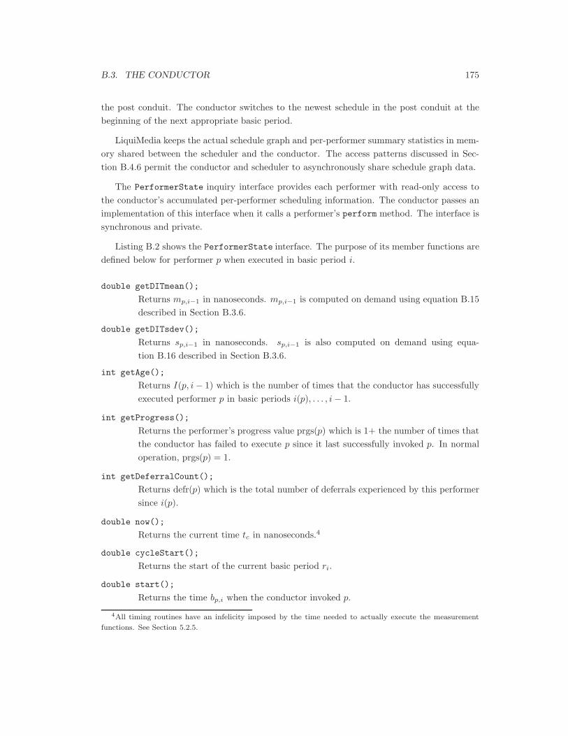
B.3. THE CONDUCTOR 175
the post conduit. The conductor switches to the newest schedule in the post conduit at thebeginning of the next appropriate basic period.
LiquiMedia keeps the actual schedule graph and per-performer summary statistics in mem-ory shared between the scheduler and the conductor. The access patterns discussed in Sec-tion B.4.6 permit the conductor and scheduler to asynchronously share schedule graph data.
The PerformerState inquiry interface provides each performer with read-only access tothe conductor’s accumulated per-performer scheduling information. The conductor passes animplementation of this interface when it calls a performer’s perform method. The interface issynchronous and private.
Listing B.2 shows the PerformerState interface. The purpose of its member functions aredefined below for performer p when executed in basic period i.
double getDITmean();
Returns mp,i−1 in nanoseconds. mp,i−1 is computed on demand using equation B.15described in Section B.3.6.
double getDITsdev();
Returns sp,i−1 in nanoseconds. sp,i−1 is also computed on demand using equa-tion B.16 described in Section B.3.6.
int getAge();
Returns I(p, i− 1) which is the number of times that the conductor has successfullyexecuted performer p in basic periods i(p), . . . , i− 1.
int getProgress();
Returns the performer’s progress value prgs(p) which is 1+ the number of times thatthe conductor has failed to execute p since it last successfully invoked p. In normaloperation, prgs(p) = 1.
int getDeferralCount();
Returns defr(p) which is the total number of deferrals experienced by this performersince i(p).
double now();
Returns the current time tc in nanoseconds.4
double cycleStart();
Returns the start of the current basic period ri.
double start();
Returns the time bp,i when the conductor invoked p.
4All timing routines have an infelicity imposed by the time needed to actually execute the measurement
functions. See Section 5.2.5.

176 APPENDIX B. ARCHITECTURE DETAILS
A performer can use the methods of PerformerState to adjust its behaviour appropriately.Consider the following examples.
• A video decompressor detects that it has been deferred in the previous basic period whengetProgress() returns 2. Fortunately it maintains a buffer of two frames so does notdrop any frames. It decompresses the current frame and selects an alternate branch ofthe schedule graph with its return code where a second performer refills the buffer withthe result of decompressing an additional video frame.5
• A realtime video compositing package contains a performer which renders particle systemsparks and blends them onto a video stream. The number of particles varies randomly.The performer constrains its running time by rendering particles until
now()− start() > .2TB.
The conductor uses the performer notification interface to notify applications of performersuspensions. Each performer instance must implement getNotifierConduit(). If this methodreturns a non-null conduit, the conductor writes a message containing an error code and areference to the offending performer when suspending the performer for any of the followingreasons: the performer returned an invalid value, it caused an overtime, its prgs(p) exceededa configurable maximum or, its defr(p) exceeded a configurable maximum.
These notification messages permit applications to adjust their schedule graphs. Considerthe following examples.
• An audio effects application consists of some number of performers performing audiofiltering and some supervisory composers. One composer listens for messages from theaudio-processing performers. If it receives any, it displays a warning dialog to the user.The dialog indicates that the application is having difficulty meeting its processor needsand permits the user to alter the relative importance of applications in the system.
• In a realtime 3D simulation such as a game, the renderer is divided into a pair of per-formers: the “core” renderer and the “glitz” renderer. The core renderer runs first andthe glitz renderer runs immediately afterward. The core renderer listens for overtime er-ror messages from the glitz renderer. Figure B.2 shows the application’s schedule graphwith three levels of “glitz” rendering. The application wishes to maximize the glitz level.
If the core renderer receives a notification indicating that the glitz renderer has experi-enced an overtime in the previous basic period, its return code specifies the next lowercost glitz performer and requests that a non-realtime application thread re-submits thesuspended high glitz performer to the schedule.
5While a performer object may only occur once in any path through the scheduling graph, two performer
objects may execute the same underlying code.
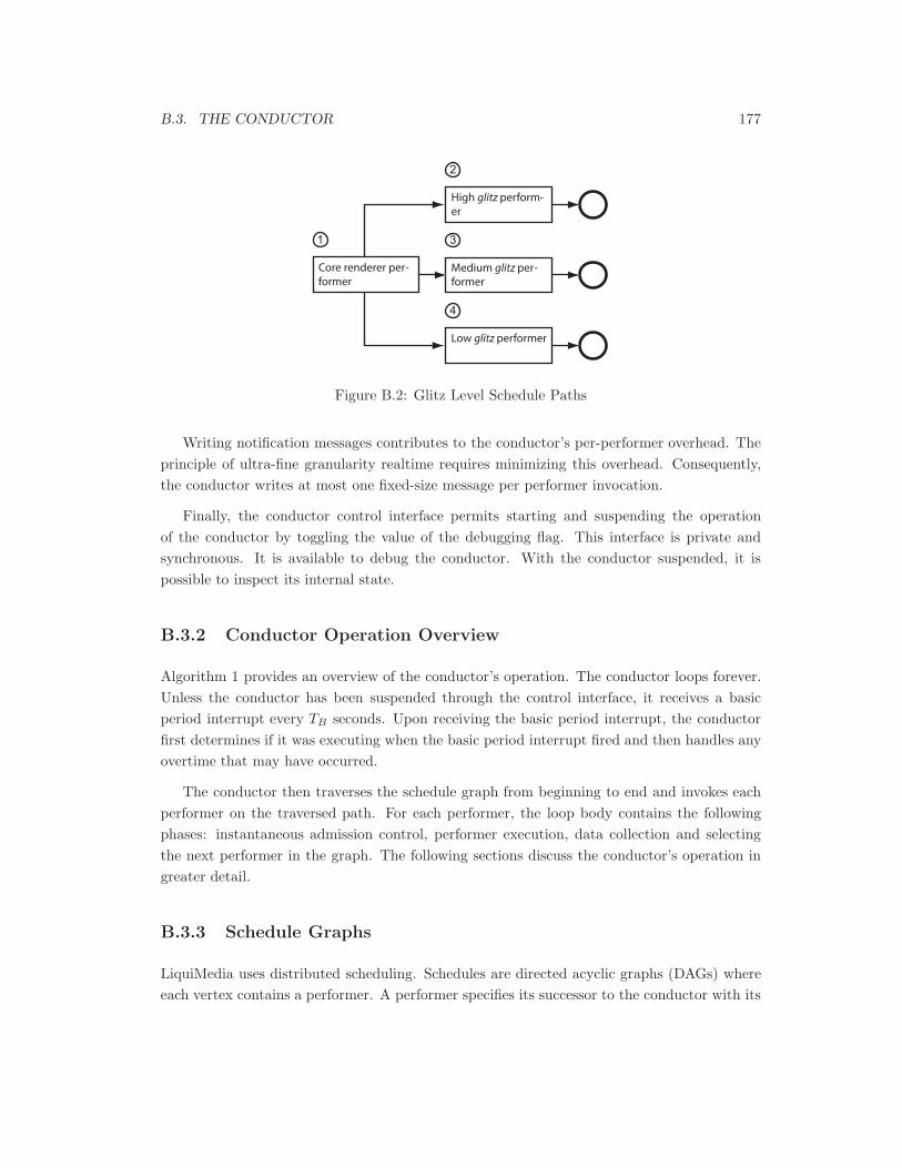
B.3. THE CONDUCTOR 177
Core renderer per-former
Medium glitz per-former
High glitz perform-er
Low glitz performer
1
2
4
3
Figure B.2: Glitz Level Schedule Paths
Writing notification messages contributes to the conductor’s per-performer overhead. Theprinciple of ultra-fine granularity realtime requires minimizing this overhead. Consequently,the conductor writes at most one fixed-size message per performer invocation.
Finally, the conductor control interface permits starting and suspending the operationof the conductor by toggling the value of the debugging flag. This interface is private andsynchronous. It is available to debug the conductor. With the conductor suspended, it ispossible to inspect its internal state.
B.3.2 Conductor Operation Overview
Algorithm 1 provides an overview of the conductor’s operation. The conductor loops forever.Unless the conductor has been suspended through the control interface, it receives a basicperiod interrupt every TB seconds. Upon receiving the basic period interrupt, the conductorfirst determines if it was executing when the basic period interrupt fired and then handles anyovertime that may have occurred.
The conductor then traverses the schedule graph from beginning to end and invokes eachperformer on the traversed path. For each performer, the loop body contains the followingphases: instantaneous admission control, performer execution, data collection and selectingthe next performer in the graph. The following sections discuss the conductor’s operation ingreater detail.
B.3.3 Schedule Graphs
LiquiMedia uses distributed scheduling. Schedules are directed acyclic graphs (DAGs) whereeach vertex contains a performer. A performer specifies its successor to the conductor with its

178 APPENDIX B. ARCHITECTURE DETAILS
Algorithm 1 Conductor Operationbasic period i← 0debugging-halt ← 0loop
Wait for a basic period interrupt5: Reentrant interrupt handler, phase one (c.f. section B.3.7)
i← i + 1ri ← tc
if debugging-halt = 1 thenBlock basic period interrupt
10: Break to debuggerend ifif basic period i− 1 completed normally thenGc ← newest posted schedule.
end if15: p← first(Gc(i)) (c.f. section B.3.3)
while p = ∅ dobp,i ← tc
if p passes instantaneous admission control test (c.f. B.3.5) theninvoke performer p
20: ep,i ← tc
tp,i ← ep,i − bp,i
r ← p’s return valueUpdate statistical profile data (c.f. section B.3.6)
end if25: p← S(p, i) (c.f. section B.3.4)
end whileti ← tc − ri
Update whole-schedule profile data (c.f. section B.3.6)if verify Gc at N(Gc, i(Gc), i) then
30: request verification of Gc
end ifend loop
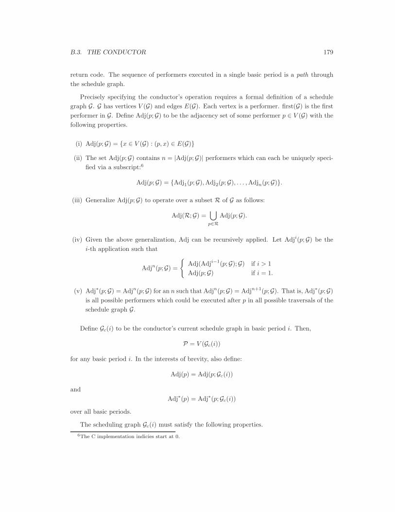
B.3. THE CONDUCTOR 179
return code. The sequence of performers executed in a single basic period is a path throughthe schedule graph.
Precisely specifying the conductor’s operation requires a formal definition of a schedulegraph G. G has vertices V (G) and edges E(G). Each vertex is a performer. first(G) is the firstperformer in G. Define Adj(p;G) to be the adjacency set of some performer p ∈ V (G) with thefollowing properties.
(i) Adj(p;G) = {x ∈ V (G) : (p, x) ∈ E(G)}
(ii) The set Adj(p;G) contains n = |Adj(p;G)| performers which can each be uniquely speci-fied via a subscript:6
Adj(p;G) = {Adj1(p;G), Adj2(p;G), . . . , Adjn(p;G)}.
(iii) Generalize Adj(p;G) to operate over a subset R of G as follows:
Adj(R;G) =⋃
p∈RAdj(p;G).
(iv) Given the above generalization, Adj can be recursively applied. Let Adji(p;G) be thei-th application such that
Adjn(p;G) =
{Adj(Adji−1(p;G);G) if i > 1Adj(p;G) if i = 1.
(v) Adj∗(p;G) = Adjn(p;G) for an n such that Adjn(p;G) = Adjn+1(p;G). That is, Adj∗(p;G)is all possible performers which could be executed after p in all possible traversals of theschedule graph G.
Define Gc(i) to be the conductor’s current schedule graph in basic period i. Then,
P = V (Gc(i))
for any basic period i. In the interests of brevity, also define:
Adj(p) = Adj(p;Gc(i))
andAdj∗(p) = Adj∗(p;Gc(i))
over all basic periods.
The scheduling graph Gc(i) must satisfy the following properties.6The C implementation indicies start at 0.
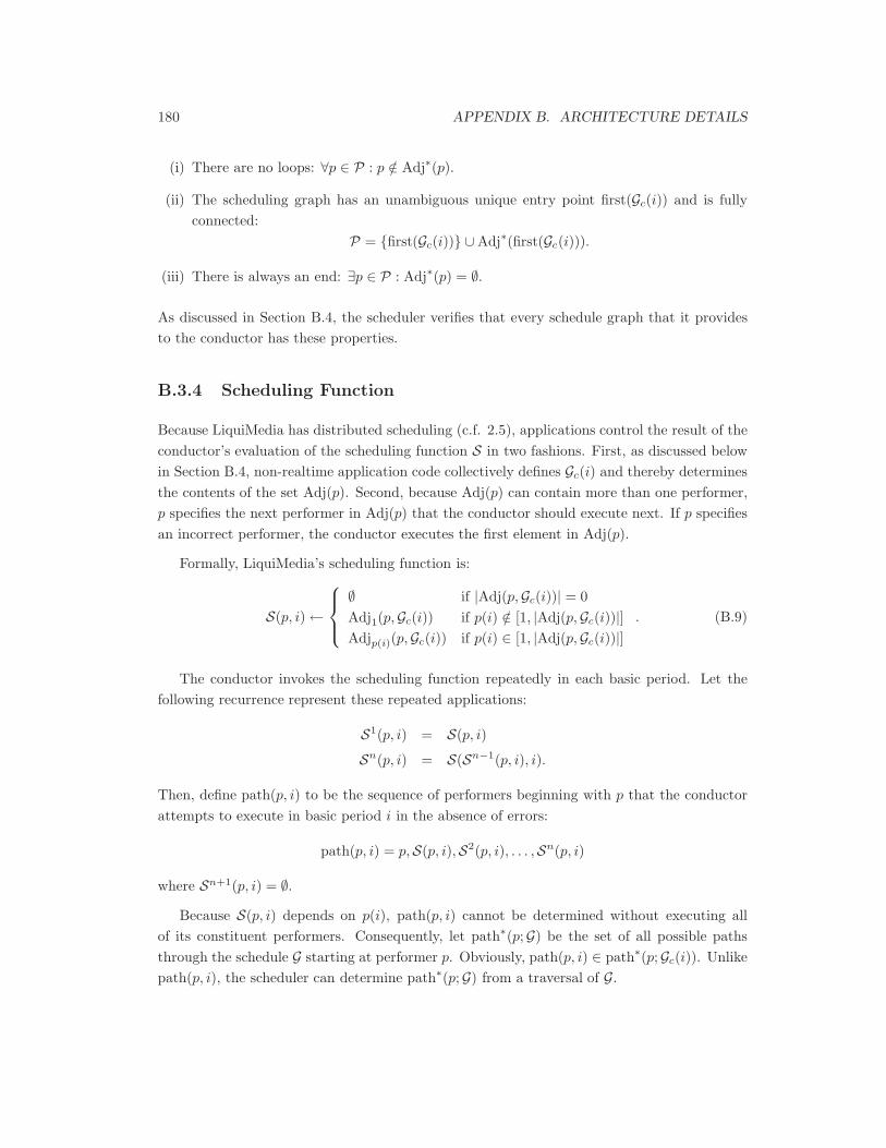
180 APPENDIX B. ARCHITECTURE DETAILS
(i) There are no loops: ∀p ∈ P : p /∈ Adj∗(p).
(ii) The scheduling graph has an unambiguous unique entry point first(Gc(i)) and is fullyconnected:
P = {first(Gc(i))} ∪Adj∗(first(Gc(i))).
(iii) There is always an end: ∃p ∈ P : Adj∗(p) = ∅.
As discussed in Section B.4, the scheduler verifies that every schedule graph that it providesto the conductor has these properties.
B.3.4 Scheduling Function
Because LiquiMedia has distributed scheduling (c.f. 2.5), applications control the result of theconductor’s evaluation of the scheduling function S in two fashions. First, as discussed belowin Section B.4, non-realtime application code collectively defines Gc(i) and thereby determinesthe contents of the set Adj(p). Second, because Adj(p) can contain more than one performer,p specifies the next performer in Adj(p) that the conductor should execute next. If p specifiesan incorrect performer, the conductor executes the first element in Adj(p).
Formally, LiquiMedia’s scheduling function is:
S(p, i)←
∅ if |Adj(p,Gc(i))| = 0Adj1(p,Gc(i)) if p(i) /∈ [1, |Adj(p,Gc(i))|]Adjp(i)(p,Gc(i)) if p(i) ∈ [1, |Adj(p,Gc(i))|]
. (B.9)
The conductor invokes the scheduling function repeatedly in each basic period. Let thefollowing recurrence represent these repeated applications:
S1(p, i) = S(p, i)
Sn(p, i) = S(Sn−1(p, i), i).
Then, define path(p, i) to be the sequence of performers beginning with p that the conductorattempts to execute in basic period i in the absence of errors:
path(p, i) = p,S(p, i),S2(p, i), . . . ,Sn(p, i)
where Sn+1(p, i) = ∅.Because S(p, i) depends on p(i), path(p, i) cannot be determined without executing all
of its constituent performers. Consequently, let path∗(p;G) be the set of all possible pathsthrough the schedule G starting at performer p. Obviously, path(p, i) ∈ path∗(p;Gc(i)). Unlikepath(p, i), the scheduler can determine path∗(p;G) from a traversal of G.
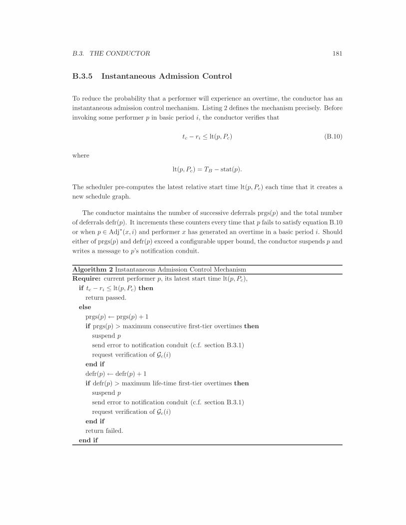
B.3. THE CONDUCTOR 181
B.3.5 Instantaneous Admission Control
To reduce the probability that a performer will experience an overtime, the conductor has aninstantaneous admission control mechanism. Listing 2 defines the mechanism precisely. Beforeinvoking some performer p in basic period i, the conductor verifies that
tc − ri ≤ lt(p, Pc) (B.10)
where
lt(p, Pc) = TB − stat(p).
The scheduler pre-computes the latest relative start time lt(p, Pc) each time that it creates anew schedule graph.
The conductor maintains the number of successive deferrals prgs(p) and the total numberof deferrals defr(p). It increments these counters every time that p fails to satisfy equation B.10or when p ∈ Adj∗(x, i) and performer x has generated an overtime in a basic period i. Shouldeither of prgs(p) and defr(p) exceed a configurable upper bound, the conductor suspends p andwrites a message to p’s notification conduit.
Algorithm 2 Instantaneous Admission Control MechanismRequire: current performer p, its latest start time lt(p, Pc),
if tc − ri ≤ lt(p, Pc) thenreturn passed.
elseprgs(p)← prgs(p) + 1if prgs(p) > maximum consecutive first-tier overtimes then
suspend p
send error to notification conduit (c.f. section B.3.1)request verification of Gc(i)
end ifdefr(p)← defr(p) + 1if defr(p) > maximum life-time first-tier overtimes then
suspend p
send error to notification conduit (c.f. section B.3.1)request verification of Gc(i)
end ifreturn failed.
end if
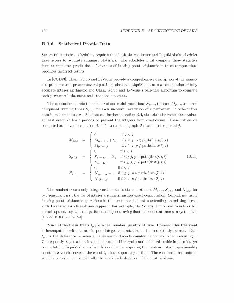
182 APPENDIX B. ARCHITECTURE DETAILS
B.3.6 Statistical Profile Data
Successful statistical scheduling requires that both the conductor and LiquiMedia’s schedulerhave access to accurate summary statistics. The scheduler must compute these statisticsfrom accumulated profile data. Naive use of floating point arithmetic in these computationsproduces incorrect results.
In [CGL83], Chan, Golub and LeVeque provide a comprehensive description of the numer-ical problems and present several possible solutions. LiquiMedia uses a combination of fullyaccurate integer arithmetic and Chan, Golub and LeVeque’s pair-wise algorithm to computeeach performer’s the mean and standard deviation.
The conductor collects the number of successful executions Np,i,j , the sum Mp,i,j, and sumof squared running times Sp,i,j for each successful execution of a performer. It collects thisdata in machine integers. As discussed further in section B.4, the scheduler resets these valuesat least every H basic periods to prevent the integers from overflowing. These values arecomputed as shown in equation B.11 for a schedule graph G reset in basic period j.
Mp,i,j =
0 if i < j
Mp,i−1,j + tp,i if i ≥ j, p ∈ path(first(G), i)Mp,i−1,j if i ≥ j, p /∈ path(first(G), i)
Sp,i,j =
0 if i < j
Sp,i−1,j + t2p,i if i ≥ j, p ∈ path(first(G), i)Sp,i−1,j if i ≥ j, p /∈ path(first(G), i)
Np,i,j =
0 if i < j
Np,i−1,j + 1 if i ≥ j, p ∈ path(first(G), i)Np,i−1,j if i ≥ j, p /∈ path(first(G), i)
(B.11)
The conductor uses only integer arithmetic in the collection of Mp,i,j , Sp,i,j and Np,i,j fortwo reasons. First, the use of integer arithmetic insures exact computation. Second, not usingfloating point arithmetic operations in the conductor facilitates extending an existing kernelwith LiquiMedia-style realtime support. For example, the Solaris, Linux and Windows NTkernels optimize system-call performance by not saving floating point state across a system-call[DN99, BBD+98, GC94].
Much of the thesis treats tp,i as a real number quantity of time. However, this treatmentis incompatible with its use in pure-integer computation and is not strictly correct. Eachtp,i is the difference between a hardware clock-cycle counter before and after executing p.Consequently, tp,i is a unit-less number of machine cycles and is indeed usable in pure-integercomputation. LiquiMedia resolves this quibble by requiring the existence of a proportionalityconstant a which converts the count tp,i into a quantity of time. The constant a has units ofseconds per cycle and is typically the clock cycle duration of the host hardware.

B.3. THE CONDUCTOR 183
Value Bound Prototype
Mp,i,j log2HTB
a 37
Sp,i,j log2 H(
TB
a
)2 61Ip,i,j log2 H 14
Table B.1: Overflow-free Integer Sizes
Values of H (basic periods), TB (time) and the proportionality constant a (time/cycle)determine machine integer sizes whose range guarantees that Mp,i,j, Sp,i,j and Np,i,j do notoverflow. Table B.1 contains formulas for the needed bit width and the actual widths neededin the liqui prototype where a is 1ns, TB is 13ms and H is 9123.
A single 64-bit integer can accommodate any one of liqui’s summary statistics withoutoverflow. With processor clock speeds exceeding 1GHz, this is no longer the case. Fortunately,integers larger that the host’s native machine integer size have only a small performancepenalty. For example, on the Intel X86 architecture, a single addition operation takes 2n
assembly language instructions to add together two 32n-bit integers [Int99]. A high-qualityassembly language implementation on a 3GHz Pentium4 could compute the 96-bit Sp,i,j in 6(short) clock cycles.
The scheduler uses Chan, Golub and LeVeque’s pair-wise approach to combine the Mp,i,i(G),Sp,i,i(G) and Np,i,i(G) collected for schedule G with floating point summary statistics np,i(G)−1,mp,i(G)−1 and s2
p,i(G)−1. Let the float() operator convert an integer value to a floating pointnumber. The scheduler computes the total number of times that some performer p has executedsuccessfully:
n(p, i) = n(p, i(G)− 1) + float(Np,i,i(G)) (B.12)
and letting
x = n(p, i(G)− 1) (B.13)
y = float(Np,i,i(G)) (B.14)
in the interests of compactness, it computes the following recurrences for the mean and vari-ance:
mp,i =1
x + y
(xmp,i(G)−1 + float(Mp,i)
)(B.15)
s2p,i =
1x + y
(xs2
p,i(G)−1
+float(
Sp,i − 1yM2
p,i
)
+x
y(x + y)
(y
mp,i(G)−1− float(Mp,i)
)2)
. (B.16)
184 APPENDIX B. ARCHITECTURE DETAILS
This approach has an error bound of κu log(x+ y) for machine accuracy u where κ has thefollowing approximation
κ ≈ mp,i/sp,i.
when sp,i is small compared to mp,i and the number of basic periods is large. Because bothof these conditions hold, the pair-wise algorithm is numerically sound and generates summarystatistics sufficiently accurate for successful statistical scheduling.
As discussed in section B.1, each performer must provide estimates to the scheduler ofits mean and standard deviation. Equations B.15 and B.16 show that LiquiMedia does notrequire that these initial estimates be correct. From the first schedule re-verification onward,LiquiMedia schedules p only on its actual running times. In order to support the execution ofuntrusted independently-authored realtime performers, LiquiMedia trusts application code aslittle as possible. Conscientious programmers should however still provide best-guess values ofa performer’s running time, typically through experience with running their code.
Internally, LiquiMedia may, as required in the interests of an efficient implementation, usea platform-specific unit for all timing statistics. Consequently, all application-level interfacesretrieve or set time values in a double precision floating point number of nanoseconds. I namedthis format Device Independent Time or DIT. Each implementation must provide appropriateconversion code from DIT to Device Dependent Time or DDT values. This conversion is trivialin the prototype as its DDT format is an integer count of nanoseconds.
B.3.7 Reentrant Operation
Sometimes the conductor has not completed executing when it receives the next basic periodinterrupt. Consequently, the conductor must support re-entrant operation. This complicatesthe conductor’s implementation. If still executing, the conductor can be in one of four differentstates upon receipt of a basic period interrupt.
(i) Interrupt i + 1 takes place before the execution of the first performer.
(ii) Interrupt i + 1 takes place between the execution of p and S(p, i).
(iii) Interrupt i + 1 takes place while executing performer p. In this case, p has experiencedan overtime.
(iv) Interrupt i + 1 takes place after the completion of all performers in path(1, i).
Ideally, the conductor would block the basic period interrupt except while actually executingperformers. This eliminates all but case (iii). Not all hardware and parent RTOSs permitthis simplification. Further, disabling and re-enabling the basic period interrupt for every

B.3. THE CONDUCTOR 185
performer invocation can impose performance penalties not compatible with the principleof ultra-fine granularity. For example, disabling the basic period interrupt in the LiquiMediaprototype takes time similar to the running time of an audio shaping performer. Consequently,algorithm 3 and algorithm 4 define the conductor’s recovery from all four types of reentrantinvocation.
Assume that performer p attempts to execute past ri+1 in basic period i. Then, theconductor should increment the deferral count for all performers x ∈ path(S(p, i), i) at thebeginning of basic period i + 1. However, path(S(p, i), i) cannot be determined. Instead, asshown in listing 4, the conductor notifies all x ∈ Adj∗(p;Gc(i)) by incrementing prgs(x) anddefr(x) and writing a message to x’s notification conduit.
As a result, having experienced a reentrant interrupt in basic period i, the conductornotifies all performers
y ∈ Adj∗(p;Gc(i))− path(S(p, i), i)
in error. LiquiMedia requires applications to correctly handle spurious notifications.
Two reasons reduce the needed development effort. First, the conductor never notifiessimple performers in error where a simple performer is one which is in every path through thecurrent schedule graph.
Second, every complex application scheduling graph such as the one shown in Figure 4.7has a simple first performer (1 in the diagram). This performer must already specify whichof performers Adj(1) = {2, 3, 8, 10} should execute next. The additional development effortneeded for performer 1 to manage the wrongly incremented progress values of its successors issmall.
Deferrals pose an additional problem. For example, if performer 1 in figure 4.7 experiencesa deferral, which of performers should 2, 3, 8, 10 execute next? In the LiquiMedia prototype,the conductor executes Adj1(p) after deferring p. The conductor proceeds identically when ithas suspended p in a previous basic period. An application can take advantage of this policyto define a schedule graph which handles performer suspensions or deferrals.
A related issue with overtimes is whether or not suspending one of an application’s per-formers should result in suspending all of them. Suspending sibling performers can be desirablebut is complex to implement and can significantly increase the conductor’s execution overhead.For these reasons, the LiquiMedia prototype does not suspend the sibling performers of a per-former that has experienced an overtime. The notification conduit provides adequate supportfor applications to submit updated schedule graphs. Because a complete schedule graph isregularly reassembled from per-application contributions as discussed below in Section B.4.4,this simpler approach does not leave orphaned performers in the schedule beyond the nextreverification.
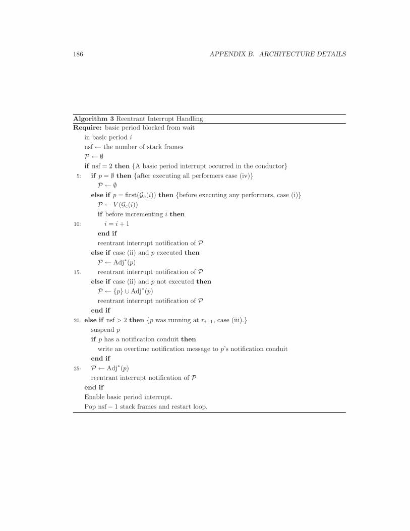
186 APPENDIX B. ARCHITECTURE DETAILS
Algorithm 3 Reentrant Interrupt HandlingRequire: basic period blocked from wait
in basic period i
nsf← the number of stack framesP ← ∅if nsf = 2 then {A basic period interrupt occurred in the conductor}
5: if p = ∅ then {after executing all performers case (iv)}P ← ∅
else if p = first(Gc(i)) then {before executing any performers, case (i)}P ← V (Gc(i))if before incrementing i then
10: i = i + 1end ifreentrant interrupt notification of P
else if case (ii) and p executed thenP ← Adj∗(p)
15: reentrant interrupt notification of Pelse if case (ii) and p not executed thenP ← {p} ∪Adj∗(p)reentrant interrupt notification of P
end if20: else if nsf > 2 then {p was running at ri+1, case (iii).}
suspend p
if p has a notification conduit thenwrite an overtime notification message to p’s notification conduit
end if25: P ← Adj∗(p)
reentrant interrupt notification of Pend ifEnable basic period interrupt.Pop nsf− 1 stack frames and restart loop.

B.3. THE CONDUCTOR 187
Algorithm 4 Reentrant Interrupt Notificationfor x ∈ P do
prgs(x)← prgs(x) + 1defr(x)← defr(x) + 1if prgs(x) > maximum consecutive deferrals then
5: suspend x.if x has a notification conduit then
write x and maximum consecutive deferral error to notification conduit (c.f. sec-tion B.3.1)
end ifelse if defr(x) > maximum life-time deferrals then
10: suspend x.if x has a notification conduit then
write x and maximum life-time error to notification conduit (c.f. section B.3.1)end if
else15: if x has a notification conduit then
write x, “deferred by other’s second-tier” message to x’s conduit (c.f. section B.3.1)end if
end ifrequest re-verification of Gc(i)
20: end for

188 APPENDIX B. ARCHITECTURE DETAILS
ApplicationScheduleStateApplicationScheduleState
Gc(i)cndt(G)
cndt(Ak)Ak Ak+1 ...
Persistent Scheduler State
Transient Scheduler State Conductor State
Shared Pool of Performer Objects
Figure B.3: The figure shows the data structures shared between the conductor, scheduler andapplications.
B.4 Scheduler
LiquiMedia’s scheduler prepares schedules from which the conductor executes performers. Thescheduler is a continuously running composer task started when LiquiMedia boots. Its oper-ation can be divided into four stages: waiting to service re-verification requests, assemblingper-application schedule graphs into a single complete schedule graph, admission-testing thissingle schedule graph and, should the new schedule be admissible, delivering it to the conduc-tor.
B.4.1 Schedule Data Structures
The scheduler’s operation depends on the underlying data structures shown in Figure B.3: ashared pool of schedule graphs, performer objects and ApplicationScheduleState objects.These data structures can be categorized by their presence in the four stages of the sched-uler’s execution. The scheduler maintains its persistent data structures while waiting forre-verification requests. It augments this data with additional transient data structures whileassembling and admission-testing a new schedule graph.
The scheduler’s persistent data structures consists of a doubly-linked list of Application-ScheduleState objects. There is one such object for each running application which has

B.4. SCHEDULER 189
1.1
1.2 1.3
1.4 1.5
2.1 2.2
2.4
2.3
2.1 2.2
2.4
2.3
3.1 3.2
3.3
3.1 3.2
3.3
1.1
1.2 1.3
1.4 1.5
Gi
A1 A2 A3
Figure B.4: An example of a well-formed schedule both as per-application fragments andconnected by the scheduler into a graph Gi.
invoked the restructure method discussed below in Section B.4.4. The ApplicationSche-
duleState object for application k contains the schedule graphAk. Ak is the k-th application’scontribution to the most recently admitted schedule.
The scheduler’s transient data structures depend on the origin of a re-verification request. Ifthe scheduler awakens as a result of a request from application k, its transient data structuresinclude two additional schedule graphs. First, arg(Ak) is the schedule graph prepared byapplication k and passed by reference to the restructure method. Second, the restructure
method prepares cndt(Ak) by copying arg(Ak) and then inserting it into the Application-
ScheduleState object for application k.
The restructure method copies arg(Ak) into cndt(Ak) to insure that an applicationcannot avoid admission testing by modifying a previously submitted shared schedule grapharg(Ak). Section B.4.4 discusses the operation of the restructure method in greater detail.
In any re-verification, the scheduler’s transient data consists of the schedule graph cndt(G).As described in Section B.4.3, the scheduler assembles the per-application schedule graphs intothis graph and then applies the lifetime admission control test described in Section B.4.5. Ifscheduler can admit cndt(G), it posts the schedule to the conductor.
Figure B.4 shows an example of the assembly process for a re-structuring invoked by theconductor. The scheduler has constructed cndt(G) from the three application schedules A1,A2 and A3.
Each successful admission results in a new schedule in a sequence:
G1,G2, . . . ,Gj .
190 APPENDIX B. ARCHITECTURE DETAILS
The conductor’s current schedule Gc(i) is taken from these sequence of posted schedules. Sec-tion B.4.6 discusses the relationship between successive admitted schedules.
All of these different schedule graphs draw their nodes from an array of s Performer
objects shared between the conductor and scheduler. s Performer objects have a sub-structureimposed by the scheduler and conductor’s different access patterns to the s Performer’s fields.The scheduler initializes all of the fields. Once the s Performer object belongs to a postedschedule, fields are either entirely read-only, conductor read-write and scheduler read-only orare read-write for both the conductor and scheduler.
The first two cases require no special treatment. The third case jeopardizes correct oper-ation of the conductor and scheduler unless there is a method for safe shared access. Onlythe statistical profile data defined in equation B.11 is read-write by both the scheduler andconductor. Fortunately, its stereotyped access patterns permit a simple solution to the sharedaccess problem.
The statistical profile information is initialized by the scheduler, repeatedly updated by theconductor and eventually read and then reset by the scheduler. Multiple separate statisticalprofile objects solve the shared access problem. The scheduler first prepares a new statisticalprofile object. Then, it atomically exchanges this object’s reference for the s Performer’sexisting reference. This atomic exchange operation gives the conductor a new zeroed statisticalprofile object to update while the scheduler computes aggregate statistical summary valuesfrom the preserved snapshots.
B.4.2 Graph Construction
In the liqui prototype’s Java interface, applications schedule performers using the applicationprogramming interface (API) discussed below in Section B.4.4. The methods comprising thisAPI take a reference to a schedule graph as an argument. An application k defines its schedulegraph argument arg(Ak) by creating instances of the ScheduleGraph class. This class has thefollowing methods.
ScheduleGraph(Performer p, String name)
This constructor creates a new ScheduleGraph instance A with
V (A) = {p}
and naming it name. The name parameter is optional. Each of the other methodsbelow operate on an instance A of ScheduleGraph.
ScheduleGraph set(ScheduleGraph A1, int i)
Adds an edge to E(A) such that
Adji(first(A);A) = first(A1).
B.4. SCHEDULER 191
ScheduleGraph get(int i)
Returns the ScheduleGraph wrapping performer Adji(first(A);A).
ScheduleGraph add(ScheduleGraph A1)
Adds an edge (first(A, first(A1)) to E(A) at the lowest unused index. This methodis a convenience for the common case of a single outbound edge or the addition ofadjacencies in order.
Performer getPfmer()
Returns the performer first(A).
ScheduleGraph find(String name)
Returns the ScheduleGraph with the given name.
An application developer uses these methods to define an application schedule graph. Forexample, the execution of the code in Listing B.3 creates the application schedule graph A2
shown in Figure B.4.
B.4.3 Schedule Assembly
All schedule re-verification operations require the scheduler to assemble cndt(G) from per-application contributions. This section precisely defines the assembly process. Schedule as-sembly assumes that each application schedule graph satisfies the properties discussed in sec-tion B.3.3.
Let the ⊕ operator concatenate two schedule graphs such that if
G = Aj ⊕Ak
then
V (G) = V (Aj) ∪ V (Ak)
E(G) = E(Aj) ∪E(Ak))
∪⋃
∀p∈Leaf(Aj)
{(p, first(Ak))}
where Leaf(Aj) is a function returning the leaf nodes of Aj and is defined as follows:
Leaf(G) = {∀x ∈ V (G) : ∀y ∈ V (G), (x, y) /∈ E(G)} .
Given the above definition of ⊕, a candidate schedule G assembled from k applicationschedule graphs is
G =k⊕
κ=1
Aκ.

192 APPENDIX B. ARCHITECTURE DETAILS
Listing B.3: Use of ScheduleGraph Class
import com . l i qu imed ia . ap i ;
class MakeGameSchedule {class CoreRenderer implements Performer {
/∗ 2.1 ∗/}class HighGlitzRenderer implements Performer {
/∗ 2.2 ∗/}class LowGlitzRenderer implements Performer {
/∗ 2.4 ∗/class Globa lL ight ingPass implements Performer {
/∗ 2.3 ∗/}
ScheduleGraph sg ;public MakeGameSchedule ( ) {
ScheduleGraph g lp = createScheduleGraph (new Globa lL ight ingPass ( ) ) ;
sg = createScheduleGraph (new CoreRenderer ( ) ) . add (createScheduleGraph (new HighGlitzRenderer ( ) ) . add (
g lp ) ) . add (createScheduleGraph (new LowGlitzRenderer ( ) ) . add ( g lp ) ) ;
// Attempt to schedu l e sg . . .}
}

B.4. SCHEDULER 193
Listing B.4: Scheduler Interface
package com . l i qu imed ia . ap i ;
public interface Scheduler {public f ina l static int FAILED = 0 ;public f ina l static int POSTED = 1 ;public f ina l static int TOOSLOW = 2 ;public f ina l static int BAD GRAPH = 3 ;
public int r e s t r u c t u r e ( ScheduleGraph k , Conduit c ) ;public int r e s t r u c t u r e ( ScheduleGraph k ) ;
}
The assembly algorithm itself consists of fundamental graph algorithms: Leaf(G) is the set ofleaves of a spanning tree produced by a breadth first search of G while actually connecting theapplication graphs consists of adding the necessary edges to the candidate graph’s adjacencylists.
B.4.4 Restructuring
An application modifies the scheduling of its performers with one of two different interfaces.The Scheduler interface shown in Listing B.4 permits an application to restructure its schedulegraph while the PrivilegedScheduler interface discussed below permits a privileged appli-cation to modify the relative importance of applications.
Graph Restructuring
Application code adds, alters or removes performers from the schedule with the restructure(ScheduleGraph k, Conduit c) method from the Scheduler interface. Typically, an appli-cation takes the following steps to modify its schedule of running performers.
(i) The application creates or modifies an existing application candidate schedule grapharg(Ak) out of instances of ScheduleGraph class as discussed in section B.4.1.
(ii) The application invokes the restructuremethod with argument arg(Ak) and an optionalconduit on which the application can receive messages from the scheduler.
(iii) The restructure mechanism executes Algorithm 5.
194 APPENDIX B. ARCHITECTURE DETAILS
(iv) The application handles any errors which might have occurred as indicated by restructure’sreturn code.
(v) The application waits on conduit c or any notification conduits that it may have specifiedfor its performers.
Algorithm 5 restructure OperationRequire: Argument arg(Ak), optional conduit c
if arg(Ak) fails to satisfy graph properties discussed in Section B.3.3 thenreturn BAD GRAPH
end ifif application did not provide conduit c then
c← temporary conduit from scheduler to applicationend iffor p ∈ V (arg(Ak))− V (Ak) do
allocate s Performer object p.initialize s Performer p.
end forV (cndt(Ak))← ∅E(cndt(Ak))← ∅for p ∈ V (arg(Ak)) do
V (cndt(Ak))← V (cndt(Ak)) ∪ s Performer corresponding to p
end forE(cndt(Ak))← E(arg(Ak))post cndt(Ak) to schedulerresponse ← c (blocks on c)return response
The restructure method executes synchronously inside the application thread. Uponinvocation, it first verifies that arg(Ak) is a valid application candidate schedule graph. If so,restructure creates an internal copy cndt(Ak). LiquiMedia confines these operations to thesubmitting application’s thread. This insures that a hostile application cannot interfere withthe scheduler by submitting a deliberately malformed application candidate schedule. Finally,the restructure method makes a restructuring request by passing cndt(Ak) to the schedulerand waits for the scheduler’s response.
The scheduler responds to the restructuring request by re-assembling all of the applicationschedules other than application k’s candidate. It assembles them in order of descending im-portance. Lastly, it appends the candidate schedule cndt(Ak) after all of the other un-modifiedapplication schedule graphs. The scheduler then applies LiquiMedia’s lifetime admission con-trol test on the resulting candidate schedule graph. If the candidate is admissible, the scheduler
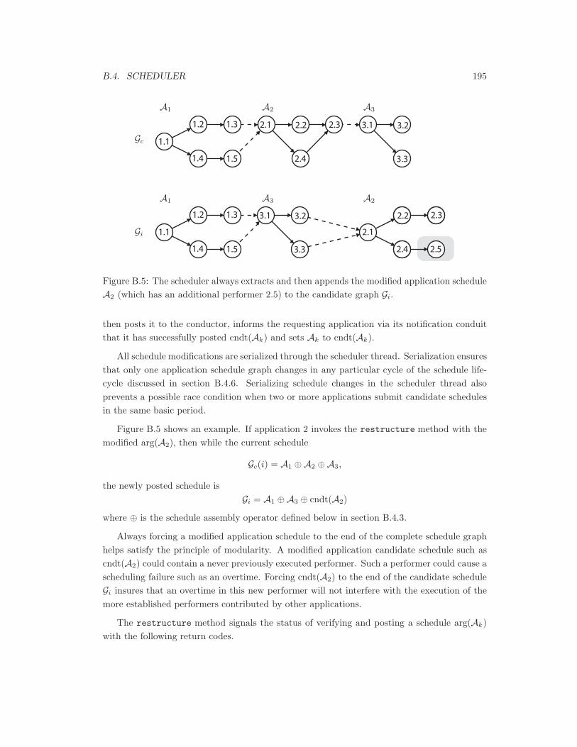
B.4. SCHEDULER 195
1.1
1.2 1.3
1.4 1.5
2.1 2.2
2.4
2.3 3.1 3.2
3.3
Gi 1.1
1.2 1.3
1.4 1.5
2.1
2.2 2.3
2.4 2.5
2.2
2.4
2.33.1 3.2
3.3
Gc
A1 A2 A3
A1 A3 A2
Figure B.5: The scheduler always extracts and then appends the modified application scheduleA2 (which has an additional performer 2.5) to the candidate graph Gi.
then posts it to the conductor, informs the requesting application via its notification conduitthat it has successfully posted cndt(Ak) and sets Ak to cndt(Ak).
All schedule modifications are serialized through the scheduler thread. Serialization ensuresthat only one application schedule graph changes in any particular cycle of the schedule life-cycle discussed in section B.4.6. Serializing schedule changes in the scheduler thread alsoprevents a possible race condition when two or more applications submit candidate schedulesin the same basic period.
Figure B.5 shows an example. If application 2 invokes the restructure method with themodified arg(A2), then while the current schedule
Gc(i) = A1 ⊕A2 ⊕A3,
the newly posted schedule isGi = A1 ⊕A3 ⊕ cndt(A2)
where ⊕ is the schedule assembly operator defined below in section B.4.3.
Always forcing a modified application schedule to the end of the complete schedule graphhelps satisfy the principle of modularity. A modified application candidate schedule such ascndt(A2) could contain a never previously executed performer. Such a performer could cause ascheduling failure such as an overtime. Forcing cndt(A2) to the end of the candidate scheduleGi insures that an overtime in this new performer will not interfere with the execution of themore established performers contributed by other applications.
The restructure method signals the status of verifying and posting a schedule arg(Ak)with the following return codes.
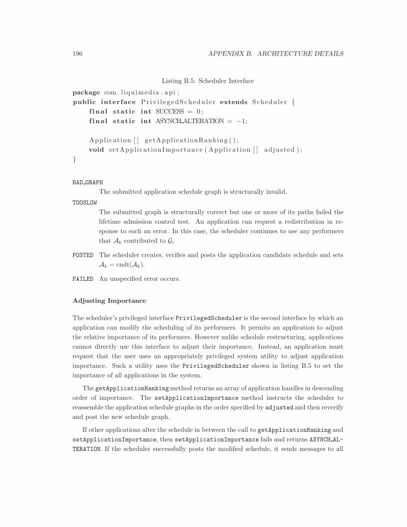
196 APPENDIX B. ARCHITECTURE DETAILS
Listing B.5: Scheduler Interface
package com . l i qu imed ia . ap i ;public interface Pr i v i l e g edSchedu l e r extends Scheduler {
f ina l static int SUCCESS = 0 ;f ina l static int ASYNCH ALTERATION = −1;
Appl i ca t ion [ ] getAppl i ca t ionRanking ( ) ;void setAppl i ca t ionImportance ( Appl i ca t ion [ ] ad justed ) ;
}
BAD GRAPH
The submitted application schedule graph is structurally invalid.
TOOSLOW
The submitted graph is structurally correct but one or more of its paths failed thelifetime admission control test. An application can request a redistribution in re-sponse to such an error. In this case, the scheduler continues to use any performersthat Ak contributed to Gc
POSTED The scheduler creates, verifies and posts the application candidate schedule and setsAk = cndt(Ak).
FAILED An unspecified error occurs.
Adjusting Importance
The scheduler’s privileged interface PrivilegedScheduler is the second interface by which anapplication can modify the scheduling of its performers. It permits an application to adjustthe relative importance of its performers. However unlike schedule restructuring, applicationscannot directly use this interface to adjust their importance. Instead, an application mustrequest that the user uses an appropriately privileged system utility to adjust applicationimportance. Such a utility uses the PrivilegedScheduler shown in listing B.5 to set theimportance of all applications in the system.
The getApplicationRankingmethod returns an array of application handles in descendingorder of importance. The setApplicationImportance method instructs the scheduler toreassemble the application schedule graphs in the order specified by adjusted and then reverifyand post the new schedule graph.
If other applications alter the schedule in between the call to getApplicationRanking andsetApplicationImportance, then setApplicationImportance fails and returns ASYNCH AL-
TERATION. If the scheduler successfully posts the modified schedule, it sends messages to all
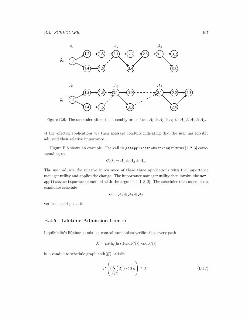
B.4. SCHEDULER 197
1.1
1.2 1.3
1.4 1.5
2.1 2.2
2.4
2.3 3.1 3.2
3.3
Gi 1.1
1.2 1.3
1.4 1.5
2.1 2.2 2.3
2.4
2.1 2.2
2.4
2.33.1 3.2
3.3
Gc
A1 A2 A3
A1 A3 A2
Figure B.6: The scheduler alters the assembly order from A1 ⊕A2 ⊕A3 to A1 ⊕A3 ⊕A2.
of the affected applications via their message conduits indicating that the user has forciblyadjusted their relative importance.
Figure B.6 shows an example. The call to getApplicationRanking returns [1, 2, 3] corre-sponding to
Gc(i) = A1 ⊕A2 ⊕A3.
The user adjusts the relative importance of these three applications with the importancemanager utility and applies the change. The importance manager utility then invokes the set-ApplicationImportance method with the argument [1, 3, 2]. The scheduler then assembles acandidate schedule
Gi = A1 ⊕A3 ⊕A2
verifies it and posts it.
B.4.5 Lifetime Admission Control
LiquiMedia’s lifetime admission control mechanism verifies that every path
X = pathi(first(cndt(G)); cndt(G))
in a candidate schedule graph cndt(G) satisfies
P
(∑p∈X
Tp) < TB
≥ Pc. (B.17)
198 APPENDIX B. ARCHITECTURE DETAILS
Section B.2.2 describes using Chebyshev’s inequality to compute an estimate of a singleperformer’s running time stat(p) with probability Pc. In a similar fashion, Chebyshev’s in-equality can estimate the running time of multiple performers and admit a schedule if itsestimated running time is less than the duration of a basic period.
Assume as a notational convenience that all the performers in cndt(G) are simple so that|path∗(first(cndt(G)); cndt(G))| = 1 and let
P = path1(first(cndt(G)); cndt(G)).
Then, the scheduler computes
stat(P) = mP,i +√
11− Pc
sP,i (B.18)
where
mP,i = wc + |P| ∗ wp +∑∀p∈P
mp,i (B.19)
sP,i =√∑
∀p∈Ps2
p,i (B.20)
and it admits the schedule cndt(G) if stat(P) < TB.
Equations B.20 and B.20 assume that the PDF of a performer’s running time is independentof the path which selected the performer for invocation. Such an assumption is valid becauseLiquiMedia expects performers to be single-function media-processing functions. Instead of asingle monolithic task containing many different behaviours, the schedule graph permits defin-ing an application’s range of operations as paths comprised of many single-function performers.LiquiMedia’s ability to schedule independently authored performers depends in part on theway that the schedule graph exposes more of an application’s structure to both the schedulerand conductor.
Algorithm 6 precisely specifies the operation of the admission control mechanism.
B.4.6 Life Cycle and Feedback
LiquiMedia’s scheduler repeats the lifetime admission control test described in section B.4.5on the running schedule Gc at intervals proportional to the schedule’s age. These additionaltests verify that Gc remains admissible after the inclusion of Mp,i,j, Sp,i,j and Np,i,j valuescollected by the conductor. If Gc fails an admission control test, the scheduler creates a newcandidate schedule and removes performers from it in order of increasing importance until thecandidate is admissible.
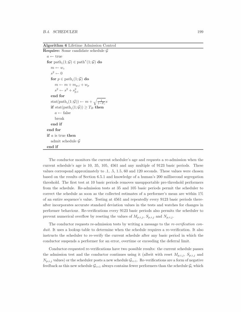
B.4. SCHEDULER 199
Algorithm 6 Lifetime Admission ControlRequire: Some candidate schedule G
a← truefor pathi(1;G) ∈ path∗(1;G) do
m← wc
s2 ← 0for p ∈ pathi(1;G) do
m← m + mp,i + wp
s2 ← s2 + s2p,i
end forstat(pathi(1;G))← m +
√1
1−Pcs
if stat(pathi(1;G)) ≥ TB thena← falsebreak
end ifend forif a is true then
admit schedule Gend if
The conductor monitors the current scheduler’s age and requests a re-admission when thecurrent schedule’s age is 10, 35, 105, 4561 and any multiple of 9123 basic periods. Thesevalues correspond approximately to .1, .5, 1.5, 60 and 120 seconds. These values were chosenbased on the results of Section 6.5.1 and knowledge of a human’s 200 millisecond segregationthreshold. The first test at 10 basic periods removes unsupportable pre-threshold performersfrom the schedule. Re-admission tests at 35 and 105 basic periods permit the scheduler tocorrect the schedule as soon as the collected estimates of a performer’s mean are within 1%of an entire sequence’s value. Testing at 4561 and repeatedly every 9123 basic periods there-after incorporates accurate standard deviation values in the tests and watches for changes inperformer behaviour. Re-verifications every 9123 basic periods also permits the scheduler toprevent numerical overflow by reseting the values of Mp,i,j , Sp,i,j and Np,i,j .
The conductor requests re-admission tests by writing a message to the re-verification con-duit. It uses a lookup table to determine when the schedule requires a re-verification. It alsoinstructs the scheduler to re-verify the current schedule after any basic period in which theconductor suspends a performer for an error, overtime or exceeding the deferral limit.
Conductor-requested re-verifications have two possible results: the current schedule passesthe admission test and the conductor continues using it (albeit with reset Mp,i,j , Sp,i,j andNp,i,j values) or the scheduler posts a new schedule Gi+1. Re-verifications are a form of negativefeedback as this new schedule Gi+1 always contains fewer performers than the schedule Gi which

200 APPENDIX B. ARCHITECTURE DETAILS
1.1
1.2 1.3
1.4 1.5
2.1 2.2
2.4
2.3 3.1 3.2
3.3
Gi
Figure B.7: The diagram outlines a path through the schedule Gi which is not admissible ingray. The scheduler attempts to make Gi by removing the boxed performer 3.3.
became the current schedule.
During the construction of any schedule Gi, the scheduler first removes all suspended per-formers. If Gi is then inadmissible, the scheduler removes performers from the ends of eachfailing path in path∗(first(Gi+1);Gi+1) until all paths pass the lifetime admission control test.
Figure B.7 shows an example of this process. pathi(1.1;Gi)’s predicted running time exceedsTB where
pathi(1.1;Gi) = {1.1, 1.4, 1.5, 2.1, 2.4, 2.3, 3.1, 3.3}.Consequently, the scheduler first removes performer 3.3. The scheduler will remove performersfrom the end of the gray path until it can admit the schedule.
The scheduler’s use of negative feedback provides a consistent and stable mechanism forimplementing importance-based scheduling. The scheduler packs the schedule with performersin decreasing order of importance. Then, over successive re-verification cycles, the conductorand the scheduler remove the lowest importance performers whose processor resource needscannot be accommodated.

Appendix C
Windows NT Scheduling Failures
Existing desktop operating systems cannot allocate processor resources in a fashion that per-mits the successful generation of realtime streams by more than one process at a time. Thisappendix describes a simple experiment that demonstrates this fact under Windows NT.
C.1 Apparatus
The experimental apparatus consisted of a dual-processor workstation running Windows NTwith sufficient memory that paging issues could be ignored. The machine has the WinAmpMP3 audio player program and the QuickTime for Windows image viewer installed. The NTPerformance monitor was used to collect results.
C.2 Procedure
The WinAmp MP3 audio player successfully generated a music stream when it was the onlyapplication generating a media stream. The human auditory system can monitor a PCMaudio stream for missing samples and can easily detect as few as three missed samples. Anysamples missing from the output stream show a scheduling failure where the audio playercannot execute before the hardware audio buffer drains. Consequently, it was easy to hearthat WinAmp decompressed the audio in realtime when it was the only multimedia applicationrunning.
Once the WinAmp audio stream was successfully established, I opened multiple images withthe QuickTime image viewer and counted the approximate number and duration of glitches inthe audio stream. The chosen images caused the image viewer to use a CODEC intended for
201

202 APPENDIX C. WINDOWS NT SCHEDULING FAILURES
decompression of DV digital video. Using the image viewer was a necessary expedient because,while a video player would have been a preferable second process, the available video playersblock at startup waiting for WinAmp to close the audio device.
C.3 Results
The digital audio player used an average of 3.2% of a processor to perform decompression.The audio stream is deeply buffered — hardware information for the machine indicates thatthe audio is fed from an 8092 byte hardware buffer, giving a minimum of 46 milliseconds ofaudio buffering before an audible glitch. This is more than three basic periods in LiquiMedia.
The image CODEC is single-threaded and uses exactly 100% of one processor. Windowingoperations such as the creation of windows to contain the decompressed images and transferthe pixels to the screen were carried out by the second processor and consumed less than 30%of its capacity.
The audio glitched reliably, with pauses approaching an appreciable fraction of a second,if the decompressor was started with at least 24 images.
The above describes a situation in which Windows NT fails to schedule two separatestream-generating processes despite adequate processing resources. Consequently, WindowsNT cannot successfully schedule all combinations of multimedia streams even when sufficientprocessor resources are available.
Appendix D
LiquiMedia Inc.
This thesis may have somewhat of a “commercial” bias: the introduction motivates the researchby its practical applications and the discussion of previous research includes numerous productsin addition to references to the academic literature. My attempt at starting a company tocommercialize the LiquiMedia technology explains this bias. This appendix provides a briefoverview of LiquiMedia Inc. (LMI) and summarizes its accomplishments.
D.1 The Company
I founded LMI in cooperation with the Eastern Technology Seed Investment Fund (ETSIF).ETSIF financed the company under the mentor capital model where ETSIF provided LMIwith both seed capital and interim management assistance.
ETSIF insisted that the company be founded before I completed the thesis in order toinsure that the public disclosure of thesis submission did not jeopardize a patent applicationon the LiquiMedia technology. In retrospect, this was an error. At first, developing the liqui
prototype benefited both the thesis and the company. However, company responsibilities suchas patent and white paper writing soon supplanted thesis work.
It was my understanding that the company’s interim management would carry out fivefundamental tasks. First, the interim management established the company’s “plumbing” —systems such a accounting and disbursement control. Second, the interim management wasresponsible for securing the company’s intellectual property. In particular, LMI applied for apatent on the LiquiMedia architecture (United State Patent Application 09/259,178).
Third, the interim management was responsible for establishing a business strategy thatcould generate revenue with a LiquiMedia-derived product. This task was a pre-requisite for
203
204 APPENDIX D. LIQUIMEDIA INC.
the two final tasks: using the revenue potential of the chosen business strategy to obtaina subsequent round of financing and hiring full-time management. The company’s interimmanagement failed to perform these tasks. With insolvency imminent, I left LMI to return towork on this thesis.1
D.2 Research
I produced all of LMI’s technical literature. This included a sizable number of technical whitepapers describing both the LiquiMedia architecture and both the advantages and defects ofrelated commercial developments. Chapter 3 discusses these products as well as results fromthe academic literature.
Working at LMI helped me develop an appreciation for the business utility of a technologysuch as LiquiMedia. While I began this thesis with nothing more than the desire to build novelmultimedia software, such an attitude is not useful in a commercial setting. An infrastructuraltechnology such as LiquiMedia has commercial value if its use improves the bottom line. Theprocessor coalescence example described in Section 1.3.2 has this potential.
D.3 Developments
LMI used the code tree developed for this thesis to implement a realtime-capable Java virtualmachine. Figure D.1 shows the general architecture. As discussed in Chapter 5, the liqui
prototype is built on top of Solaris. LMI integrated Sun’s Java virtual machine (JVM) intothe liqui prototype.
LMI’s development had two main components. First, it developed the “RTX” realtimeextension that tied together a binary-only Java virtual machine with the existing liqui pro-totype. This extension enabled Java composers to create and install Java performers into theLiquiMedia scheduler and for these code fragments to use the conduit facility. As part of thiseffort, LMI also identified a restricted subset of Java that performers could successfully use.
Second, LMI developed a audio player application in Java that would demonstrate thatLMI’s combination of LiquiMedia, Solaris and the Java virtual machine could in fact executea mixture of realtime and non-realtime fragments written in Java. The demonstrator was asimulation of a portable MP3 player, such as the Diamond RiO [Dia00]. The Java MediaFramework provided non-realtime decoding of the compressed audio. Running the JMF’sdecoder as a performer would have required access to the both the JVM and JMF sources andwould have required development effort which exceeded the available time. Java performersprovided a latency-controlled graphic equalizer and software volume control.
1The compactness of this paragraph belies the unpleasantness.

D.3. DEVELOPMENTS 205
Solaris
RTXJRE1.2
SPARC
LiquiMedia
Figure D.1: LiquiMedia Inc. Demonstrator
206 APPENDIX D. LIQUIMEDIA INC.
This combination of non-realtime decoding and realtime post-processing demonstrated thatLiquiMedia could successfully partition the operation of realtime and non-realtime tasks. Italso demonstrated the operational correctness of the conduit library. Performance data fromthe audio processing performers showed that multimedia performers have running time distri-butions similar to the Pareto distribution where statistical scheduling offers a sizable utilizationadvantage over rate monotonic scheduling.
D.3.1 Audioplayer Lessons
The implementation of the audio player provided a number of valuable practical lessons: thedifficulty of realtime development and the particular difficulty of realtime development withoutcomplete control of the infrastructure. This section discusses these lessons briefly.
First, the version of the Sun Java virtual machine used by the LMI development teammay choose to perform a garbage collection on any attempt to allocate storage. This includesthe allocation of a stack frame for a Java method invocation. The execution of all Java codeis blocked while the garbage collector runs. Garbage collection pauses typically range from30ms to 150ms. Consequently, Java performers in the LMI realtime JVM must minimize theirmemory allocations. Insuring that collections did not interfere with Java performer executionwas the foremost difficulty in obtaining realtime execution of Java code in the LMI JVM.
Second, Solaris 2.6 does not implement priority inheritance in a single process contain-ing realtime and non-realtime kernel threads. This complicated the conductor’s support forreentrant operation.
Third, the Sun audio device driver uses Streams [Bac86]. The keyboard and mouse driversalso use Streams. Interlocks inside the stream stack can deadlock the kernel when realtimeand non-realtime threads in kernel context contest for access to in-kernel stream functionality.
Finally, LiquiMedia’s statistical admission control and full support for reentrant operationin the conductor were invaluable for bringing realtime to Java. The combination of Java’sgarbage collection and its inter-operation with the remainder of Solaris make the JVM arealtime-uncooperative environment. Java performers have exceedingly long tails in their run-ning time distributions. Statistical scheduling’s tolerance for such “messy” distributions wasessential to successfully execute Java performers in realtime.
D.4 Summary
Working at LMI was extremely educational. It provided an opportunity to evaluate the thesisresearch against criteria atypical for academic work: its potential for commercial application.The LiquiMedia technology has sizable commercial applicability — it can lower overall system

D.4. SUMMARY 207
costs for devices that must execute several multimedia tasks. However, commercializing a bodyof research requires management, marketing and business development skills that computerscience coursework failed to provide.


Appendix E
PDF Statistical Scheduling
Appendix B presented a detailed description of how LiquiMedia uses Chebyshev’s inequalityto compute its estimate of a performer’s running time stat(p) with at least some minimumprobability Pc. Use of Chebyshev’s inequality permits computing stat(p) for an arbitraryperformer.
Chebyshev’s inequality does not provide the tightest possible bound stat(p). Estimatingstat(p) using p’s true probability distribution function (PDF) φp(t) provides the smallest possi-ble value of stat(p). However, φp(t) cannot be determined. This appendix discusses PDF-styleestimation: the use of a function φp(t) to approximate the unknown φp(t). It also shows thatthe normal distribution is a poor choice for φp(t).
E.1 PDF-style Estimation
Assume that there exists some PDF φp(t) which when parametrized with p’s (full-sequence)mean µp and standard deviation σp satisfies equation E.1 with at least Pg probability.
P (φp(t; µp, σp) ≈ φp(t)) ≤ Pg (E.1)
Then, stat(p) is the solution of equation E.2.
∫ t=stat(p)
t=0
φp(t; µp, σp)dt =Pg
Pc(E.2)
Solving equation E.2 for stat(p) would produce a much smaller value of stat(p) than theone estimated by equation B.5 if equation E.1 holds with probability Pg > Pc. Consequently,PDF-style estimation requires a two step process: the scheduler first verifies that equation E.1holds and then solves equation E.2.
209

210 APPENDIX E. PDF STATISTICAL SCHEDULING
Verifying equation E.1 is a classical problem in statistics: test the hypothesis that φ(t; µp, σp)fits p’s actual running times tp,1, . . . tp,i for i invocations of performer p. I chose the rank scorestechnique for this verification as it permits using linear regression to evaluate how well a non-linear function fits a sample [WM78].
Embedding this verification process into LiquiMedia complicates the implementation asthe conductor must collect and preserve a sample window of per-invocation running times foreach performer. Further, the scheduler must include code to compute a linear regression onthe sample versus its rank scores. This hypothesis verification step alone has a considerablylarger memory footprint and scheduler execution overhead than the entire resource use of theChebyshev-style estimator. Consequently, its impact on the principle of ultra-fine granularityis only justified if its per-performer utilization benefits exceed the increased scheduler overhead.
Having completed the first verification step, the scheduler must actually compute a valueof stat(p). Given an integrable function φp(t) such that
Φp(t) =∫
φp(t)dt
then equation E.2 can be re-expressed (note that the probability of performer execution times≤ 0 is 0) as shown in equation E.3.
stat(p) = Φ−1p;µp,σp
(Pg
Pc) (E.3)
The scheduler repeatedly computes the values of stat(p) for hundreds or even thousands ofperformers and so the choice of φp(t) must permit the scheduler to efficiently compute equa-tion E.3.
As with the use of Chebyshev’s inequality, the values of µp and σp are not available. Thefunction φp(t) must instead be parametrized with a sample mean and standard deviationcorrected as discussed in section B.2.2.
E.2 Normal Distribution
Successful PDF-style estimation requires a choice of function for φp(t). The normal distributionwarranted investigation as a possible choice for two reasons. First, as required by the centrallimit theorem, the distribution of the combined running times of many performers (such as asingle path through the schedule graph) will tend to be normally distributed as the number ofperformers increase [WM78]. Second, it is easy to numerically solve equation E.3 for stat(p)when using the normal distribution as the function φp(t).
However, the normal is a poor estimator of the standard test performers discussed inChapter 6 and will fare even worse for realistic performers as they have large positive skewand resemble a Pareto distribution.

E.2. NORMAL DISTRIBUTION 211
Running Time Simple Synth Jittered Sinusoidal.01 .325 .278 .572 .742.05 .523 .695 .852 .952.10 .641 .763 .964 .975.20 .774 .868 .971 .975.40 .871 .894 .992 .966.75 .667 .943 .980 .955
Table E.1: Normal Score Correlations
I evaluated the normal distribution’s ability to estimate a performer’s running time byproducing normal score plots for the standard test performers. The correlation between the n
normal scores ν1, . . . , νn and the actual performer runtime data tp,1 . . . tp,n where
νi = Gau−1(i− 1/3n + 1/3
)
and Gau−1 is the inverse normal cumulative distribution function provides a numerical measureof how closely a normal distribution approximates the running time of a performer p. If thesample distribution is perfectly normal, the normal score would be 1.0.
Table E.1 summarizes the correlation between the performers’ normal scores and theiractual running times. While an appropriate distribution to estimate a performer’s runningtime might improve processor utilization, the normal distribution is not a sufficiently goodestimator of performer run time to warrant its use. For example, for .40 Jittered, the performerwith the most normally distributed run time distribution, at Pc = .99, the normal providesonly a 8% tighter bound than using Chebyshev’s inequality.
In the case of .01 Simple, the normal estimator provides a 20% tighter stat(p) than theChebyshev-style estimator. However, with a correlation between its normal scores and sampledistribution of .325, the tighter bound is specious.
Obviously the normal distribution is not a good choice for φp(t). Many other possible dis-tributions exist. For example, the Pareto distribution ought to be a better choice [AB98b]. Re-gardless of the chosen distribution’s ability to fit the actual performer invocation running times,the greater complexity of the PDF-style estimator’s two-phase verification process favours theuse of the Chebyshev-style estimator. Further, the two-phase verification process may unfairlyreject performers whose running time distribution does not match the chosen approximatingPDF. Consequently, use of PDF-style estimation is only warranted when the operating sys-tem domain requires maintaining high utilization levels at values of Pc above those needed bymultimedia applications.

Appendix F
Testing Summary
F.1 Introduction
F.1.1 Test Performers
Almost all of the tests had the following general structure:
1. a test harness composer and
2. some number of performers drawn from the standard test performers discussed in Sec-tion 6.1.3.
F.2 Unit Testing
The following unit tests were applied to their corresponding components.
cord test.c
String handling [Boe04].
storage test.c
Instrumented storage and interfaces to garbage collector [Boe04].
closures test.c
Thread wrappers for terminating composer threads.
composer test.c
Composer task creation and cleanup.
213

214 APPENDIX F. TESTING SUMMARY
conduit test.c
Conduit asynchronous message passing facilities.
group test.c
Schedule graph structures. Schedule graphs are also re-used to store composer taskinformation in liqui.
impresario test.c
Loading of application shared libraries, initialization, composer task creation andclean-up.
lead test.c
Schedule path management.
performer test.c
Performer management data structures, creation, clean-up, statistical profile collec-tion and computation.
properties test.c
Schedule graph annotations.
schedule test.c
Scheduler, admission testing and schedule restructuring.
signalhandlers test.c
Exception handling and portions of priority inheritance.
F.3 Integration Testing
Implementation tests are pass or fail. Each test applied a stimulus to liqui while its statemet the test’s specified pre-condition. To pass, liqui satisfied the post-condition after theapplication of the stimulus. Some of the tests require liqui to correctly reach the postconditions within a bounded amount of time. Test descriptions use the notation explained inAppendix B.
1. App liqui harness, single spinning composer, debugger.
Pre A composer executing without a lock.
Stim A single basic period interrupt sent to the conductor.
Post One normal conductor iteration.
2. App liqui harness, single spinning composer, debugger.
Pre A composer executing with a locked conduit mutex.
Stim A single basic period interrupt sent to the conductor.
Post The conductor blocked on the conduit mutex.

F.3. INTEGRATION TESTING 215
3. App liqui harness, single spinning composer, debugger.
Pre A performer executing.
Stim A single basic period interrupt sent to the conductor.
Post Performer suspension code (overtime case) executed (c.f. iii).
4. App liqui harness, single spinning composer, debugger.
Pre Conductor running but not in the context of a performer.
Stim A single basic period interrupt sent to the conductor.
Post Conductor restarts without handling overtime but checks for need to incrementprogress values (c.f. i, ii, iv).
5. App empty startup.c
Pre A ready to run liqui without an application.
Stim Start liqui for a small fixed number of cycles.
Post Message log contains all service composer start and stop messages in the correctorder.
6. App chatty performer.c
Pre A running liqui with heavy-weight logging and no performers.
Stim app main creates a new group containing a single correct performer and installsit. The performer logs its invocations.
Post Message log contains all performer invocation messages.
7. App chatty performer.c
Pre A running liqui with no installed performers.
Stim app main schedules a performer which logs its age and profile.
Post Logged ages and statistical profiles are correct.
8. App seg fault performer.c
Pre One installed performer p.
Stim p generates an exception in basic period i.
Post p is suspended for an error and has no light-weight statistical profile records forbasic periods > i.
9. App basic performer.c
Pre One installed performer p.
Stim p enters an infinite loop in basic period i.
216 APPENDIX F. TESTING SUMMARY
Post At the end of conductor initialization in basic period i + 1, p is suspended(overtime) and has no light-weight records for basic periods ≥ i.
10. App multi performer.c
Pre Installed performers 1, . . . , pl.
Stim Randomly chosen p ∈ [1, pl) enters an infinite loop in basic period i.
Post p is suspended due to overtime, prgs(x) = 1; x ∈ [1, p − 1], prgs(y) = 2; y ∈[p + 1, pl]
11. App arbitrary delta.c
Pre Installed performer p having prgs(p) = 1 in basic period i− 1.
Stim p executes successfully in basic period i.
Post prgs(p) = 1 after completion of execution of performer p in basic period i.
12. App domino.c
Pre Installed performers 1, . . . , pl with pl greater than the maximum number ofsuccessive deferrals.
Stim p . . . p + n enter infinite loops in basic periods i . . . i + n respectively
Post At the end of basic period i + n, all performers p, . . . , p + n are suspended forovertime and all performers p+n, . . . , pl are suspended for too many successivedeferrals.
13. App ot1 test.c
Pre Installed performers 1 . . . pl.
Stim In basic period i, the aggregate running time of performers 1, . . . , p− 1 exceedslt(p, Pc).
Post At the end of basic period i, p is deferred and has prgs(p) = 2.
14. App restructuring tests.c
Pre For k admitted applications with candidate schedule contributions: A1, . . . ,Ak
such that
Gc =k⊕
κ=1
Aκ.
Stim Application i invokes schedRestructureSchedule 1.
Post Posted schedule Gi is
Gi =i−1⊕κ=1
Aκ ⊕k⊕
κ=i+1
Aκ ⊕Ai
1The C function equivalent to restructure in Section B.4.4.

F.3. INTEGRATION TESTING 217
15. App restructuring tests.c
Pre For k admitted applications with candidate schedule contributions: A1, . . . ,Ak
with performer p in some application candidate schedule Aκ
Stim In basic period i, p enters an infinite loop.
Post Posted schedule Gi does not contain performer p and application κ receives anovertime suspension notice in its notification conduit.
16. App restructuring tests.c
Pre For k admitted applications with candidate schedule contributions: A1, . . . ,Ak
such that
Gc =k⊕
κ=1
Aκ.
and un-scheduled but admissible application candidate Ak+1.
Stim Application k + 1 invokes schedRestructureSchedule.
Post Posted schedule Gi is
Gi =k+1⊕κ=1
Aκ


Appendix G
Approximating wcet(p)
Chapter 6 makes the following approximation:
wcet(p) ≈ maxi=1,...,n
tp,i
because it is impossible to actually compute maxi=1,...,n tp,i without knowing the PDF ofperformer p.
It is possible to quantify the probability that this approximation places the Chebyshev esti-mator at a disadvantage compared to the WCET estimator. For n random variables X1, . . . , Xn
selected from the PDF fp(x) of performer p, then
P (∀i ∈ [1, n]; Xi < max(x)) =n∏
i=1
P (Xi < max(x)) (G.1)
=n∏
i=1
∫ max(x)
0
fp(x)dx (G.2)
=
(∫ max(x)
0
fp(x)dx
)n
(G.3)
But in the sample of n = 4561 random variables,
P (∀i ∈ [1, n]; Xi < max(x)) =45604561
(G.4)
≈ 0.9998 (G.5)
so ∫ max(x)
0
fp(x)dx =(
45604561
)1/4561
(G.6)
≈ 0.99999995. (G.7)
219

220 APPENDIX G. APPROXIMATING WCET(P)
Consequently, given that no value of X can exceed the length of the basic period, the proba-bility that there is a X larger than max(x) is extremely small.