adoption of breeding technologies in the u.s. dairy
TRANSCRIPT
Louisiana State UniversityLSU Digital Commons
LSU Master's Theses Graduate School
2010
Adoption of breeding technologies in the U.S. dairyindustry and their influences on farm profitabilityAditya Raj KhanalLouisiana State University and Agricultural and Mechanical College, [email protected]
Follow this and additional works at: https://digitalcommons.lsu.edu/gradschool_theses
Part of the Agricultural Economics Commons
This Thesis is brought to you for free and open access by the Graduate School at LSU Digital Commons. It has been accepted for inclusion in LSUMaster's Theses by an authorized graduate school editor of LSU Digital Commons. For more information, please contact [email protected].
Recommended CitationKhanal, Aditya Raj, "Adoption of breeding technologies in the U.S. dairy industry and their influences on farm profitability" (2010).LSU Master's Theses. 1307.https://digitalcommons.lsu.edu/gradschool_theses/1307
ADOPTION OF BREEDING TECHNOLOGIES IN THE U.S.
DAIRY INDUSTRY AND THEIR INFLUENCES ON FARM
PROFITABILITY
A Thesis
Submitted to the Graduate Faculty of the
Louisiana State University and
Agricultural and Mechanical College
in a partial fulfillment of the
requirements for the degree of
Master of Science
in
The Department of Agricultural Economics and Agribusiness
by
Aditya Raj Khanal
B.Sc (Ag.), IAAS, Tribhuvan University, Nepal, 2006
December, 2010

ii
DEDICATION
To my parents Mr. Gopi Raj Khanal and Mrs. Laxmi Khanal, for their love,
inspiration, and support………..

iii
ACKNOWLEDGEMENTS
I would like to express my sincere gratitude to my major advisor, Dr. Jeffrey M. Gillespie
for his thoughtful guidance and endless support throughout my study. I was able to learn a great
deal as a protégé under his mentorship. There is no way that I can truly express my thanks to
you, Dr. Gillespie.
Appreciation is also extended to my graduate committee members, Dr. Ashok Mishra and
Dr. Michael Salassi for their insightful suggestions during my study. I would also like to thank
Dr. Krishna Paudel and Dr. Carter Hill for their help and suggestions. Thanks also go to Dr.
William Greene for quick response to my e-mails regarding LIMDEP programming.
Thanks to my family for their love and support. Thanks dad for helping me become a
person I am today, teaching me to choose right from wrong, and never letting me feel down.
Thanks to my loving mom, brothers, and sisters, for wishing my best and providing constant
support and encouragement.
I am deeply indebted to all my friends who helped me during my stay and study at LSU.
Thanks to my colleagues Arun, Narayan, Abhishek, Gnel, Sachin, Mahesh, Kashi, Deepa and
many more for their best wishes and support. I would like to thank the Nepalese community at
Baton Rouge for their love and support. I will miss you.
Finally, I am thankful to USDA, LSU AgCenter and Department of Agricultural
Economics and Agribusiness for providing me a financial support throughout my study, without
which this thesis would not be possible.

iv
TABLE OF CONTENTS
DEDICATION…………………………………………………………………………. ii
ACKNOWLEDGEMENTS………………………………………………………….....
iii
LIST OF TABLES………………………………………………………………………
vi
LIST OF FIGURES……………………………………………………………………..
vii
ABSTRACT…………………………………………………………………………......
viii
CHAPTER 1: INTRODUCTION ………………………………………………............
1
1.1. Background……………………………………………….................................. 1
1.2. Problem Definition……………………………………………………………... 6
1.3. Research Questions…………………………………………………………….. 7
1.4. Objectives…………………………………………………................................. 8
1.5. Arrangement of the Thesis……………………………………………………...
8
CHAPTER 2: LITERATURE REVIEW……………………………………………….. 9
2.1. Technology Adoption………………………………………………………….. 9
2.2. Technology Adoption in the U.S. Dairy Industry……………………………… 11
2.3. Breeding Technologies and Adoption………………………………………….. 12
2.4. Adoption and Impact Studies: Review of Methodology……………………….. 16
CHAPTER 3: DATA AND METHODOLOGY …………………………………….....
20
3.1. Data…………………………………………………………………………….. 20
3.2. Models………………………………………………………………………….. 21
3.2.1. Adoption Decision Models………………………………………………… 21
3.2.1.1. Economic and Econometric Model Set-up…………………………... 21
3.2.1.2. Statistical Test for Zero Correlation………………………………….. 28
3.2.1.3. Marginal Effects. …………………………………………………….. 28
3.2.1.4. Heteroskedasticity……………………………………………………. 29
3.2.1.5. Independent Variables Used in Adoption Equations………………… 30
3.2.2. Farm Impact Models……………………………………………………….. 34
3.2.2.1. Model Set-up…………………………………………………………. 34
3.2.2.2. Accounting for Endogeneity and Self-Selection Bias Issues………… 35
3.2.2.3. Test for Endogeneity and Overidentifying Restrictions……………... 38
3.2.2.4. Heteroskedasticity Correction………………………………………... 39
3.2.2.5. Variables in Farm Impact Models……………………………………. 40
CHAPTER 4: RESULTS AND DISCUSSION…………………………………………
45
4.1. Characteristics of Adopters and Non-Adopters………………………………... 45
4.2. Adoption Decision Model……………………………………………………… 47
4.2.1. Descriptive Statistics……………………………………………………... 47
v
4.2.2. Separate (Univariate) Probit Results……………………………………... 49
4.2.3. Test for Zero Correlation………………………………………………… 49
4.2.4. Bivariate Probit with Selection Results………………………………….. 50
4.3. Farm Impact Models………………………………………............................. 54
4.3.1. Descriptive Statistics…………………………………………………….. 54
4.3.2. Farm Impact and Cost Measures…………………………………............ 57
4.3.2.1. Net Returns Over Costs……………………………………………. 57
4.3.2.2. Milk Yield Per Cow……………………………………………….. 58
4.3.2.3. Net Returns over Costs per Unit of Input and Output……………. 60
4.3.2.4. Gross Returns on the Farm………………………………………… 64
4.3.2.5. Cost Measures on the Farm………………………………………... 66
4.3.3. Multicollinearity Diagnostic Test……………………………………….. 69
CHAPTER 5: SUMMARY AND CONCLUSIONS……………………………………
71
5.1. Summary……………………………………………………………………….. 71
5.2. Conclusions and Recommendations…………………………………………… 76
5.3. Limitations……………………………………………………………………... 78
REFERENCES………………………………………………………………………….
79
VITA…………………………………………………………………………………….
87
vi
LIST OF TABLES
4.1 Mean Differences between Breeding Technologies Adopters and Non-Adopters,
2005…………………………………………………………………………………..
46
4.2 Weighted Descriptive Statistics: Dependent and Independent Variables in Adoption
DecisionModel………………………………………………………………………..
48
4.3 Estimated Separate Probit Equations………………………………………………….
50
4.4 Estimated Bivariate Probit Model with Sample Selection…………………………….
52
4.5 Marginal Effects of the Adoption of ETSS and AI…………………………………...
53
4.6 Descriptive Statistics of Dependent Variables Used in Impact Model………………..
55
4.7 Descriptive Statistics of Independent Variables Used in Impact Model………………
56
4.8 Farm Impact: OLS Estimators of Net Returns over Total and Operating Costs, and
Milk Yield per Cow…………………………………………………………………..
59
4.9 Farm Impact: OLS Estimators of Net Returns over Total and Operating Costs per
CWT and Cow………………………………………………………………………..
61
4.10 Farm Impact: OLS Estimators of Overall Farm Revenue (Gross Returns) and Total
Costs per CWT and Cow…………………………………………………………….
65
4.11 Farm Cost Measures: OLS Estimators of Total Operating and Allocated Costs per
CWT and Cow………………………………………………………………………..
68
4.12: Results of Multicollinearity Diagnostic Test………………………………………..
70

vii
LIST OF FIGURES
1.1 Total U.S. Dairy Cows and Milk per Dairy Cow, 1990-2007………………………
1
1.2 Change in Milk Production by Farm Production Region, 1980-2003………………
2
3.1 U.S. States Covered by ARMS, Dairy Version 2005……………………………….
20
3.2 U.S. States Included Under WESTUS and SOUTHUS…………………………… 33
viii
ABSTRACT
Current trends in the U. S. dairy industry show an increase in milk cows per farm and
milk production per cow, though the total number of milk cows in the industry is declining. This
increase in productivity is attributed to advancements and adoption of modern dairy
technologies. Breeding technologies are one of the important components of this structural
change. This study analyzed the factors affecting the adoption of modern breeding technologies
such as artificial insemination, embryo transplants, and sexed semen, and the impact of these
technologies on farm productivity and profitability.
Results of a bivariate probit model with selection showed that the adoption decision is
affected by different farm and farmer attributes such as age, education, off-farm work, farm size,
and specialization. The embryo transplants and/or sexed semen technology adoption decision
was also influenced by the farmer‟s planning horizon. Farm impact was assessed by estimating
net returns and cost measures using ordinary least squares methods. Endogeneity and self-
selection bias issues were also tested and corrected for in the impact models. Both artificial
insemination (AI) and embryo transplants and/or sexed semen (ETSS) technologies are found to
have significant and positive influences on net returns over total and net returns over operating
costs per hundredweight of milk produced. Results also suggest that a higher allocated cost is
associated with ETSS adoption. Relatively younger, more highly educated farmers and larger
and more specialized farms received higher net returns. Since some part of the costs involved in
ETSS may be for conducting artificial insemination, larger farms that had already adopted AI
may consider ETSS adoption. Adoption decisions on a farm, however, would be based on the
added advantages of ETSS adoption versus the additional costs of adopting these.

1
CHAPTER 1
INTRODUCTION
1.1 Background
The U.S. dairy industry has experienced significant structural change during the last few
decades. Average U.S. herd size was 19 cows in 1970, rising to 120 in 2006 (MacDonald et al.,
2007). Over that period, average milk produced per cow doubled and milk produced per farm
increased twelvefold (MacDonald et al., 2007). Trends show that the larger, more efficient
operations are continually increasing their share of the milk cow inventory and milk production
while numbers of smaller operations are declining. The very large operations with 2,000 or more
cows doubled in number between 2000 and 2006 (MacDonald et al., 2007). In the industry,
farms with more than 1,000 cows are growing (contributing more than one third of the inventory
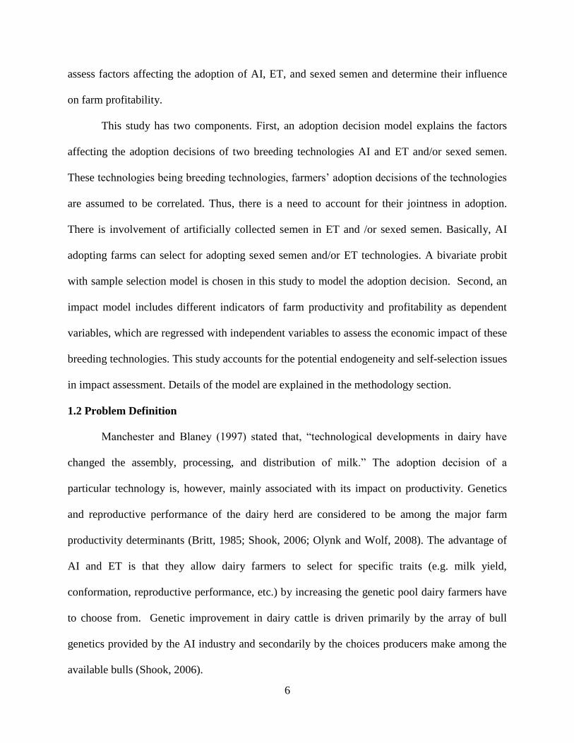
in 2004, but less than 10 percent in 1992). Figure 1.1 shows the increasing trend of milk per cow
along with a decline in the cow population over the years.
Source: USDA/ NASS
Figure 1.1: Total U.S. Dairy Cows and Milk per Dairy Cow, 1990-2007
8,400
8,600
8,800
9,000
9,200
9,400
9,600
9,800
10,000
10,200
1990 1995 2000 2005
Year
Dair
y C
ow
s (
1,0
00 h
d)
0
5,000
10,000
15,000
20,000
25,000
Mil
k P
er
Co
w (
lbs)
Milk Cows (Average) Milk Produced per Cow

2
Geographically, milk production has increased in the western United States where herd
size is relatively larger. However, traditional dairy states are also rapidly increasing their
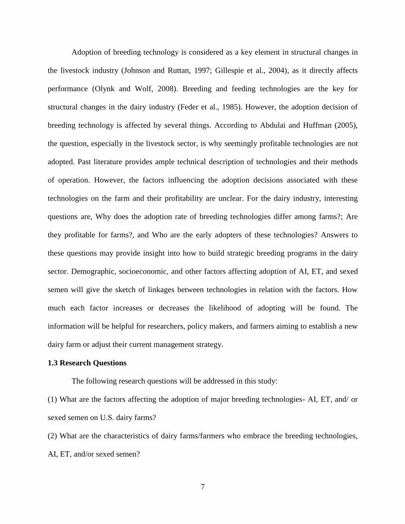
numbers of larger operations (Short, 2004). Figure 1.2 compares the milk production between
1980 and 2003, showing the changes in milk production across different regions.
Note: Units are millions of pounds of milk. Source: USDA, Report to Congress, July, 2004.
Figure 1.2: Change in Milk Production by Farm Production Region, 1980-2003
Total annual milk production in 2008 is reported at around 180 billion pounds (189,992
million pounds), an increase of 2.3 percent from 2007 (USDA/NASS, 2009). Average milk
production per cow in 2008 was 20,396 pounds which is an increase of 501 pounds per cow from
2006 (USDA/NASS, July 2009). The report also shows that the dairy industry generated cash
receipts of $34.8 billion from 189 billion pounds of milk marketed in 2008. Regarding regional
3
production, the Pacific region (25.63%) was the highest contributor of total U.S. milk production
in 2006, followed by Lake States (21.38%) (ERS, USDA, 2009).
Remarkable specialization and mechanization over the years have been key factors
associated with structural changes (Short, 2000; Short, 2004; MacDonald et al., 2007).
MacDonald et al. (2007) found that the return from large dairy enterprises well exceeds their full
costs while smaller dairy farms incur economic losses if capital cost and time contribution of the
owners are included. This ongoing structural change of shifting production to larger operations
will continue putting downward pressure on dairy prices (MacDonald et al., 2007), forcing
smaller operations out of the industry (Short, 2004).
New technology is always a critical element in a changing industry structure. Johnson
and Ruttan (1997) found breeding technologies as the most significant factor contributing to
farm productivity in the livestock sector since the 1940s. Dairy was the first livestock sector to
accept the concept of commercial breeding (Johnson and Ruttan, 1997). The dairy industry has
experienced a substantial increase in milk produced per cow, mostly attributed to innovations in
breeding and feeding systems (MacDonald et al., 2007).
Breeding technologies are among the important components of structural change in the
U.S. dairy industry. Modern dairy cows with higher production potential have been developed
through genetic selection. This is consistent with the findings of Short (2004), who indicated a
relatively large proportion of farms used genetic selection and breeding programs to improve
herd quality. On the other hand, higher yielders require greater management; failing to recognize
this fact may result in financial loss (Britt, 1985). There appears to be a direct relationship
between herd management and reproductive performance, ultimately influencing farm profit
(Britt, 1985). According to Shook (2006), genetics has accounted for about 55% of gains in the
yield traits and about one-third of the change in the time interval required to conception. This
4
can be accomplished through artificial insemination (AI), embryo transplants (ET), sexed semen
and/or traditional breeding methods. This thesis addresses adoption rates of AI as well as ET and
sexed semen.
Artificial insemination is a breeding process in which sperm collected from the male are
processed, stored and artificially introduced into the female. Artificial insemination has become
one of the most important techniques for genetic improvement of farm animals. Literature has
shown the significant impact of AI in dairy cattle (Barber, 1983; Hillers et al., 1982). Artificial
insemination has made maximum use of superior sires, allowing a good economic return (Hillers
et al., 1982).
Embryo Transplant is a technique by which embryos are collected from a donor female
and are transferred to recipient females. Recipients do not have genetic influence on the embryo.
Multiple eggs may be obtained from a cow via hormone administration, even with young heifer
calves. These “superovulated,” generally more valuable donor cows are then inseminated and
embryos are allowed to grow for 4-5 days prior to their being transferred to relatively less
valuable recipient cows (Tyler and Ensminger, 2005). Application of ET results in an increase in
the reproductive rate of females. An increase in such rate is an opportunity to reduce the number
of dams that need to be selected for the next generation (Arendonk and Bijma, 2003).
Sexed semen technology comprises the separation of sperm into male/Y bearing and
female/X bearing sperm cells and then artificially inseminating with the desired sexed-sorted
semen. Sexed semen technology lets dairy producers increase the supply of replacement heifers,
resulting in lower purchase cost of heifers. Using sexed semen, a calf of specific sex can be
produced (De Vries, et al., 2008); however, slower sorting speed and lower conception rate (35
to 40% with sexed semen as compared with 55 to 60% for unsexed semen) are the main
limitations (Weigel, 2004).
5
Artificial insemination, after its introduction in 1940s, gained a rapid initial diffusion
(Johnson and Ruttan, 1997). Considering its positive influence on genetic improvement and
profitability, AI is one of the farmer-friendly and widely adopted breeding technologies (Johnson
and Ruttan, 1997; Hillers et al., 1982; Barber, 1983). Embryo transplants and sexed semen
technologies are relatively newer and still diffusing technologies on dairy farms. Embryo
transplant technology was used at the farm level after the development of non-surgical methods
in 1970s. Studies suggested that the application of ET could produce a substantial genetic
improvement and increase in reproductive rate of females (De-Boer and Arendonk, 1994;
Arendonk and Bijma, 2003). Use of sexed semen technology on farms is increasing. Application
of sexed semen allows sorting the semen and lets dairy farmers increase the supply of
replacement heifers, resulting in lower purchase cost of heifers. Sexed semen technology is
suggested to have a wider adoption and impact in the near future (Weigel, 2004; De Vries et al.,
2008).
Farmers‟ technology adoption decisions are generally affected by a number of
demographic and socioeconomic factors. In an economic sense, farmers adopt technology if the
utility associated with adopting it is greater than the utility associated with not adopting. Feder et
al. (1985) suggested that changes in parameters affecting farmers‟ decisions are the result of
dynamic processes such as information gathering, learning by doing, or accumulating resources.
Adoption of breeding technologies such as AI, ET, and sexed semen has significant
economic value in dairy performance (De Vries et al., 2008; Seidel 1984). Despite their
influence on productivity, a number of factors cause the rate of adoption of these technologies to
be different across dairy farms. This study uses extensive survey data (Agricultural Resource
Management Survey- Dairy Version) of the United States Department of Agriculture (USDA) to
6
assess factors affecting the adoption of AI, ET, and sexed semen and determine their influence
on farm profitability.
This study has two components. First, an adoption decision model explains the factors
affecting the adoption decisions of two breeding technologies AI and ET and/or sexed semen.
These technologies being breeding technologies, farmers‟ adoption decisions of the technologies
are assumed to be correlated. Thus, there is a need to account for their jointness in adoption.
There is involvement of artificially collected semen in ET and /or sexed semen. Basically, AI
adopting farms can select for adopting sexed semen and/or ET technologies. A bivariate probit
with sample selection model is chosen in this study to model the adoption decision. Second, an
impact model includes different indicators of farm productivity and profitability as dependent
variables, which are regressed with independent variables to assess the economic impact of these
breeding technologies. This study accounts for the potential endogeneity and self-selection issues
in impact assessment. Details of the model are explained in the methodology section.
1.2 Problem Definition
Manchester and Blaney (1997) stated that, “technological developments in dairy have
changed the assembly, processing, and distribution of milk.” The adoption decision of a
particular technology is, however, mainly associated with its impact on productivity. Genetics
and reproductive performance of the dairy herd are considered to be among the major farm
productivity determinants (Britt, 1985; Shook, 2006; Olynk and Wolf, 2008). The advantage of
AI and ET is that they allow dairy farmers to select for specific traits (e.g. milk yield,
conformation, reproductive performance, etc.) by increasing the genetic pool dairy farmers have
to choose from. Genetic improvement in dairy cattle is driven primarily by the array of bull
genetics provided by the AI industry and secondarily by the choices producers make among the
available bulls (Shook, 2006).
7
Adoption of breeding technology is considered as a key element in structural changes in
the livestock industry (Johnson and Ruttan, 1997; Gillespie et al., 2004), as it directly affects
performance (Olynk and Wolf, 2008). Breeding and feeding technologies are the key for
structural changes in the dairy industry (Feder et al., 1985). However, the adoption decision of
breeding technology is affected by several things. According to Abdulai and Huffman (2005),
the question, especially in the livestock sector, is why seemingly profitable technologies are not
adopted. Past literature provides ample technical description of technologies and their methods
of operation. However, the factors influencing the adoption decisions associated with these
technologies on the farm and their profitability are unclear. For the dairy industry, interesting
questions are, Why does the adoption rate of breeding technologies differ among farms?; Are
they profitable for farms?, and Who are the early adopters of these technologies? Answers to
these questions may provide insight into how to build strategic breeding programs in the dairy
sector. Demographic, socioeconomic, and other factors affecting adoption of AI, ET, and sexed
semen will give the sketch of linkages between technologies in relation with the factors. How
much each factor increases or decreases the likelihood of adopting will be found. The
information will be helpful for researchers, policy makers, and farmers aiming to establish a new
dairy farm or adjust their current management strategy.
1.3 Research Questions
The following research questions will be addressed in this study:
(1) What are the factors affecting the adoption of major breeding technologies- AI, ET, and/ or
sexed semen on U.S. dairy farms?
(2) What are the characteristics of dairy farms/farmers who embrace the breeding technologies,
AI, ET, and/or sexed semen?

8
(3) Are these technologies profitable for U.S. dairy farms? What is the impact of adoption of AI
and ET and /or sexed semen techniques on U.S. dairy farms?
1.4 Objectives
This thesis research has the following objectives:
To determine the factors affecting the adoption of breeding technologies on US dairy
farms.
To determine the impact of AI, and ET, and/or sexed semen techniques on the
productivity and profitability of U.S. dairy farms.
1.5 Arrangement of the Thesis
Chapter 2 provides a review of literature on adoption of technology. Chapter 3 describes the
data, conceptual model, and methodological frameworks used in this study. Chapter 4 presents
and discusses the results obtained. Finally, Chapter 5 provides summary and conclusions.
9
CHAPTER 2
LITERATURE REVIEW
2.1 Technology Adoption
In a general sense, adoption may be viewed as an act of accepting as approval, accepting
or choosing or taking something as your own. Rogers (1995) defines adoption of an innovation
as the mental process of decision making that begins with hearing about the innovation to its
final adoption. Five stages of the adoption process include knowledge, persuasion, decision,
implementation and confirmation (Rogers, 1995). Initial adoption is generally followed by
diffusion, the spread of the technology within a region (Feder et al., 1985).
Extensive literature can be found regarding technology adoption on farms. Griliches
(1957), on the economics of technological change associated with hybrid corn, was one of the
early economic studies on adoption and diffusion. Feder et al. (1985) extensively surveyed
theoretical and empirical studies regarding the patterns of adoption behavior, focusing on
developing countries. They suggested that changes in the parameters that affect farmers‟
decisions are the result of dynamic processes such as information gathering, learning by doing or
accumulating resources. The adoption decision of a farmer is based upon the maximization of
expected utility subject to constraints such as limited resources including land, credit, etc. Farmer
experience, the information gathered from previous periods, information about indicators (such
as yield, profit, revenue) accumulated over periods, and information obtained by other farmers
are used in further making the decision about the technology (Feder et al., 1985).
Besley and Case (1993) focused on understanding technology adoption across space and
time and developed empirical models for studying technological adoption. Ghosh et al. (1994)
studied technology adoption and its relationship with technical efficiency and risk attitude. A
10
number of factors have been identified as influencing technology adoption. Massey et al. (2004)
found that factors relating to the farm business (financial stability, level of debt, etc.); efficiency
of the innovation system (presence of extension and consultancy providers, the availability of
information, the ease with which individuals can access information, etc.); and individual
characteristics (age, education, confidence, and innovation capacity) affect technological
learning on the basis of their survey of the New Zealand Dairy industry. Rogers (1995)
classified adopters into innovators, early adopters, early majority, late majority and laggards
based on the adoption decisions they make. Massy et al. (2004) extensively reviewed the
literature regarding early adopters, suggesting that adoption will happen quickly if the individual
is better educated, receptive to new ideas, self-confident and younger, and the farm system is
large, profitable, endowed with absorptive capacity, able to transplant information, and linked
with other farms and networks.
Bandiara and Rasul (2006) studied farmers‟ adoption choices in relation to their social
network. If there were few adopters in a network, the social effect would be positive; the effect,
however, is negative with many adopters (Bandaira and Rasul, 2006). Abdulai and Huffman
(2005) studied diffusion of cross-bred cows in Tanzania, finding that the effects among farmers
are stronger for smaller than for larger areas. Credit availability and contact with extension
agents are correlated with adoption (Abdulai and Huffman, 2005). However, in the context of
Mozambique, Bandiara and Rasul (2006) wrote, “….giving incentives to adopt early to too many
farmers can actually reduce the incentives to adopt for other farmers around them.”
Abdulai et al. (2008) examined the decision of dairy farmers to acquire information and
adopt technology in the presence of uncertainty in Tanzania. They found that human capital and
scale of operation were positive and significant in the adoption decision. Increases in education,
11
age and herd size, and an expectation of higher profitability from the technology were found to
have positive effects on adoption intensity.
2.2 Technology Adoption in the US Dairy Industry
Technology adoption in dairy is an important element of structural change in the industry.
Johnson and Ruttan (1997) reviewed the structure of the dairy industry. They revealed that
during the 1980s, increased production, slow growth in consumption, and lower government
support prices in the dairy sector led farms to increase in size. This also shifted dairy production
from the traditional areas where average herd size was 50 to 150 head (Lake States, Northeast) to
the Pacific, Mountain and Southern Plain regions (herd sizes of 500 to 1500 cows). Hammond
(1994) explains that in traditional dairy states such as Wisconsin and Minnesota, farms with herd
sizes of 100 or more increased their herd sizes while smaller farms declined in number. Weersink
and Tauer (1991) showed, however, that the direction of casualty appeared to be from herd size
to technology; their finding partially supported the view of productivity change as the cause of
change in size.
Technological developments in dairy have changed the assembly, processing, and
distribution of milk (Manchester and Blayney, 1997).Various studies related to dairy farm cost
efficiency have shown that the adoption of production practices or technologies impact
profitability. Foltz and Chang (2002), El-Osta and Johnson (1998), and similar studies have
found production per cow to be a strong factor associated with dairy farm profitability. Studies
have also shown that inferior genetics, low quality feeds, and disease incidence are limiting
factors for production per cow. El-Osta and Morehart (2000) showed that the chance of a farmer
being in the lowest quartile of production performance is lower with the adoption of capital or
management intensive technology. Those farmers who were in the top performance group had
milk production costs 53% lower than those in the low-performance group (El-Osta and
12
Morehart, 2000). These facts demonstrate the importance of improved production practices in
dairy production. Early adoption studies in agriculture and more recently Bandiera and Rasul
(2006) have shown that agricultural innovations are adopted slowly and some aspects of the
agricultural adoption process are yet to be understood. Feder et al. (1985) mentioned that the
new technologies have attained only partial success even though new technology often offers an
opportunity to increase production and income substantially. Many questions regarding the
determinants of technology adoption are not easily answered (Besley and Case, 1993), especially
in the livestock sector (Abdulai and Huffman, 2005). This leads to further enthusiasm about the
factors affecting technology adoption in the dairy sector.
2.3 Breeding Technologies and Adoption
The application of reproductive and breeding techniques has a major impact on the
structure of breeding programs, genetic gain and the dissemination of the genetic gain in
livestock production (Arendonk and Bijma, 2003). According to Shook (2006), genetics has
accounted for about 55% of gains in the yield traits and about one-third of the change in the time
interval required to conception. This can be accomplished through AI, ET, sexed semen and
traditional breeding methods.
The dairy sector was the first to adopt improved breeding for commercial production in
the livestock sector. Breeding and herd improvement associations had an important role in
disseminating information about AI after its introduction in the 1940s (Johnson and Ruttan,
1997). Artificial Insemination was introduced at the local level. The industry experienced a rapid
initial diffusion of the technology (Johnson and Ruttan, 1997). In the past 50 years, AI developed
as a solution for the need for genetic improvement and elimination of costly venereal diseases
(Foote, 1996). Hillers et al. (1982) compared the cost and returns of breeding dairy cows both
artificially and naturally. The study clearly showed the economic advantage of using genetically
13
superior AI bulls in breeding. This study showed that calving intervals with natural service (NS)
in excess of 365 days or an initial conception rate of AI greater than 0.5 would make AI
economically more favorable compared to NS. In addition, there is the risk of personal injury
using NS due to the presence of bulls. Management factors such as accuracy of estrus detection
and knowledge of proper insemination techniques are the constraints to even wider use of AI
(Hillers et al., 1982). Barber (1983) found both biological and monetary factors affecting the
adoption of breeding technologies. For most commercial dairy herds, Barber (1983) outlined the
dramatic impact of AI on genetic improvement and profitability. Busem and Bromley (1975)
showed the adoption of new breeding technology to be closely linked with stability of farm
income. Steady cash flow is their major source of income in intensively managed dairy
enterprises. An AI breeding program could be recommended for dairy operations (Barber, 1983).
Foltz and Chang (2002), El-Osta and Johnson (1998), and other studies have found production
per cow as a strong factor associated with dairy farm profitability.
According to Johnson and Ruttan (1997), “Breeding technologies are highly information
intensive. An understanding of the principles of breeding and genetics, as well as performance
data collection, management and analysis, are often necessary in order to use the new
technologies effectively.” They added, “Increasing knowledge can increase the effectiveness of
breeding technologies; however it also favors a large operation over which to spread the costs.”
This provides some intuition about the factors affecting the adoption of breeding technologies.
There are differences in AI adoption rates and productivity between regions and producers.
Shumway (1987) considers the costs involved in effective AI use as one of the explanations for
differences in adoption rates and productivity among regions and producers. The farmer‟s
breeding decision is the key factor in increasing productivity through AI.
14
Application of ET technologies results in an increase in the reproductive rate of females.
An increase in this rate is an opportunity to reduce the number of dams that need to be selected
for the next generation (Arendonk and Bijma, 2003). Arendonk and Bijma (2003) referred to
research which concluded that Multiple Ovulation and Embryo Transplants (MOET) could
produce substantial increases in genetic improvement and its main advantage is faster
dissemination of superior genetics using cloned embryos (De Boer and Arendonk, 1994).
Arendonk and Bijma (2003) also illustrated that factors such as genetic scheme and genetic merit
between available semen and embryos as well as the purchase price of semen and embryos
determine a farmer‟s decision to inseminate a cow with semen from a progeny tested sire or to
implant the embryo.
Use of sexed semen will lead to higher genetic merit of the newborn calf (Arendonk and
Bijma, 2003). Weigel (2004) revealed that the use of sexed semen has been limited to a few
highly marketable animals. However, he also mentioned the keen interest of dairy producers in
acquiring sexed semen, which shows the potential high rate of adoption of this technology. De
Vries et al. (2008) mentioned that the use of sexed semen is expanding. Due to continued
improvement in fertility and sorting capacity of sexed semen, commercial application will be
wider (De Vries et al., 2008). With the use of sexed semen and better utilization of genetic
markers, cost of progeny testing and ET will be lower (De Vries et al., 2008). According to
Weigel (2004), early adopters of this technology capture economic benefits because adopters
will get an increased supply of (extra) replacement heifers and the chance to expand rapidly from
within a closed herd.
Embryo transplant technology was significantly used after the development of non-
surgical methods in the 1970s. The number of registered Holstein calves doubled yearly in
1980s, but the rate slowed after the 1980s (Hasler, 1992). Neither ET nor sexed semen
15
techniques seem to be perfectly feasible for all types of farms, thus their lack of rapid adoption
diffusion. There may be several technical and managerial reasons behind this. Structured ET
operations require a great deal of capital to build facilities (Funk, 2006). Smeaton et al. (2003)
revealed that embryo technologies have a low uptake rate in New Zealand dairy. They also
mentioned that embryo-based reproductive technologies are usually not profitable in the general
situation if the offspring obtained by ET does not command a higher price than that from natural
mating or AI systems. According to Foote (1996), ET for selected animals was successful partly
because the dairy farmers who adopted AI for generations showed their interest in applying new
methods of making desired germplasm.
Sexing sperm in a dairy enables producers to predetermine the sex of offspring prior to
conception. Seidel (1984) had explained basically two procedures of sexing embryos. The first,
„karyotyping,‟ requires biopsy and the killing of a number of embryonic cells to examine the
chromosomes. The second includes making an antibody to molecules to distinguish male
embryos from females with a florescent microscope or by an enzymatic product. Arendonk and
Bijma (2003) mentioned that the use of ET or sexed semen help farmers to reduce calving
difficulties and improve animal welfare. Medical News Today (2006) in their website (accessed
on July, 2009) reports, “Several companies providing artificial insemination to the dairy, beef
and swine industries, including some of the world's largest, have signed licensing term sheets
with Toronto-based Microbix Biosystems Inc. (TSX:MBX) for distribution of its proprietary
Sperm Sexing Technology (SST). Microbix' technology allows breeders to determine the sex of
offspring prior to the insemination of cattle or swine.” Quoting Willium J. Gastle, the president
and CEO of Microbix Company, Medical News Today (2006), "Upon commercialization, this
will be the single-greatest breakthrough since the advent of commercial artificial insemination
almost 50 years ago and will revolutionize the way animal production takes place. Our market
16
research indicates within three years of launch of this technology, close to 100 percent of the
dairy semen provided will be sexed semen." Microbix (2009) predicts that semen sales in the
dairy industry, the largest user of AI, will increase by more than 2-fold with the introduction of
sex-specific semen.
Herbst et al. (2009) studied the effects of sexed sorted semen on Southern dairy farms.
The study showed that the use of sexed-sorted semen over unsorted semen made available the
surplus replacement heifers to sell. The positive results of more heifer calves should compensate
the higher cost of sexed-sorted semen to have application of this technology in farms (Herbst et
al., 2009).
2.4 Adoption and Impact Studies: Review of Methodology
Assessing the impact of technology is the subject of discussion in some adoption models.
Various scholars have discussed and used different statistical methods to assess the actual impact
on the farm (Foltz and Chang, 2002; Fernandez-Cornejo and McBride, 2002; Tauer, 2001; Foltz
and Lang, 2005; Tauer, 2006). To assess the financial impact of a breeding technology on a farm,
we need to control the effects of several other factors that may also affect financial performance.
The effects of the other technologies and management practices, size, location and operator
characteristics need to be accounted for in order to isolate the effect of a breeding technology on
farm financial performance.
Endogeniety and self selection issues and their associated correction methods have been
discussed (for e.g., Vella and Verbeek, 1999; Green, 2005; Freedman and Sekhon, 2008). Vella
and Verbeek (1999) statistically explained that the popular two procedures in estimating the
impact of endogenous treatment effects, instrumental variables and control function procedures,
are closely related. Heckman (1978, 1979) suggested a two-step method for taking care of
endogeneity. This popular two-step method is used by many scholars in their studies. Freedman
17
and Sekhon (2008) compared the methods for removing endogeniety bias in regression. They
showed that the likelihood methods are superior to the 2SLS method in a probit model. They
stated, however, the serious numerical concerns in maximizing the bivariate probit likelihood
function by standard software packages. They also referred to the literature where maximum
likelihood functions performed rather badly.
Gillespie et al. (2004) studied the adoption of four breeding technologies in the hog
industry. They used a multivariate probit technique to estimate the impact of factors affecting
adoption. The multinomial probit technique is also possible in this case, but use of multinomial
probit becomes more difficult and complicated when more than two technologies are under study
(Gillespie et al., 2004).
Burton et al. (1999) used binomial and multinomial logit techniques to study the adoption
decision regarding organic techniques. Besides two groups-“adopters” or “non-adopters,” they
also categorized “registered-adopters” and “unregistered adopters” within adopters. They used a
likelihood ratio test to find significant differences between binomial and multinomial logit
techniques. Results suggested that there are differences between “registered” and “unregistered”
groups, suggesting that they should not be treated as homogenous.
Caswell and Zilberman (1985) studied the choices of sprinkler or drip irrigation
technologies relative to traditional surface irrigation and the factors influencing them. However,
Dorfman (1996) commented that the use of the multinomial logit model in Caswell and
Zilberman (1985) did not measure the interaction between the two improved technologies.
Dorfman (1996) used the multinomial probit model to assess the adoption decision with multiple
technologies. According to Dorfman (1996), the multinomial probit model had not been widely
used in the past because of some computational difficulties. Now, however, the computation is
easier with advances in computing methods, specifically Gibbs sampling and the use of the
18
numerical Bayesian approach in estimation. The relationship or interaction between two
technologies can also be assessed (Dorfman, 1996). Dorfman (1996) used the multinomial
probit in an adoption study of two technologies: Integrated Pest Management (IPM) and
irrigation, dividing them into four possible technology bundles as four possible adoption
decisions.
El- Osta et al. (2007) used the multinomial logit to measure the economic well-being of
U.S. farm households among four different wealth categories. They estimated the relative and
absolute well-being of households. Using least squares estimates, they also included the
probabilities of off-farm work and government payments from the first stage multinomial logit
models.
Moreno and Sunding (2003) used a bivariate probit model to estimate the simultaneous
nature of technology adoption and land allocation. They included a technology adoption equation
as a function of the crop choice decision. A bivariate probit model was estimated by maximum
likelihood.
Monero and Sunding (2005) found that technology choice differed for different crops,
though technology and crop decisions were taken jointly. So, they estimated technology adoption
using a nested logit model of technology adoption and crop choice. They showed a farmer‟s crop
technology choices as a two-level nested choice.
El-Osta and Morehart (2000) used two separate logistic regressions in a first-stage
estimation of management and capital intensive technologies. The binomial logits were used to
obtain estimated probabilities of adoption. They incorporated the predicted probabilities
(technology variables) and selectivity variables from first stage models as exogenous variables in
a second stage output frontier model to address simultaneity and self-selectivity concerns.
19
Abdulai et al. (2008) studied the adoption of technology in the presence of uncertainty
among dairy farmers of Tanzania. They jointly estimated the information acquisition and
adoption decision. They also estimated the intensity of adoption using the Heckman (1979)
procedure using bivariate probit model equations (first step) followed by use of the inverse Mills
ratio in the intensity equation. Cooper and Keim (1996) also used a selectivity model with a
bivariate probit sample selection in assessment of adoption of water quality protection practices.
Technology adoption and farm financial performance are jointly determined. Thus, there
is a simultaneity concern (Zepeda, 1994). Several studies (e.g., Fernendez-Cornejo and McBride,
2002; Foltz and Chang, 2002) have used predicted probabilities from adoption decision models
as instrumental variables in second stage impact models. They had randomly assigned farmers as
adopters and non-adopters. The farmers had decided themselves to be the adopter or non-
adopter. Thus, the adopters and non-adopters in this sense may be systematically different, which
may lead to differences in farm performance; thus there is the need to account for self-selectivity
(Greene, 1997).
Fernandez-Cornejo and McBride (2002) studied the financial impact of adoption of
genetically engineered crops. They included predicted probabilities and an inverse Mills ratio
from the first stage adoption decision model (probit) as additional regressors in a second stage
regression (impact model) to account for simultaneity and self-selectivity. Fernandez-Cornejo et
al. (2002) studied the on-farm impacts of adopting herbicide-tolerant soybean. They used
predicted probabilities from first stage probits to account for endogeneity coming from
simultaneity and self-selection bias.
20
CHAPTER 3
DATA AND METHODOLOGY
3.1 Data
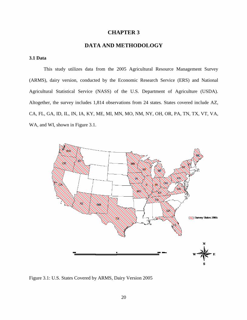
This study utilizes data from the 2005 Agricultural Resource Management Survey
(ARMS), dairy version, conducted by the Economic Research Service (ERS) and National
Agricultural Statistical Service (NASS) of the U.S. Department of Agriculture (USDA).
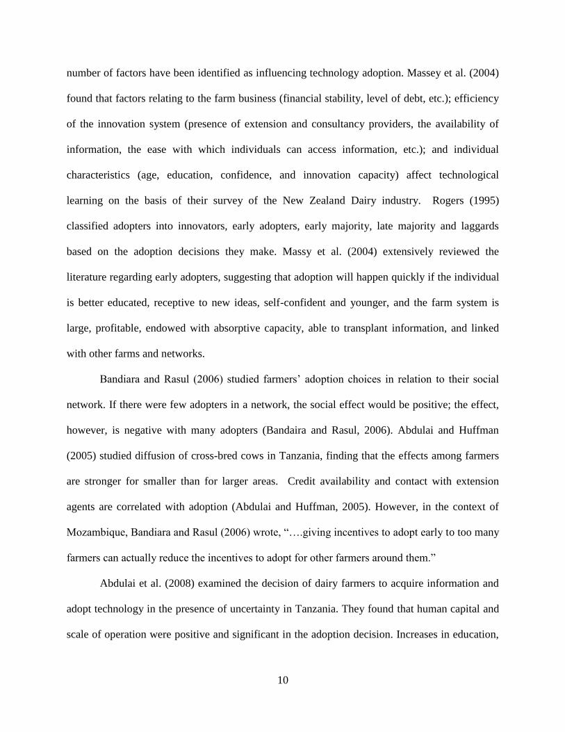
Altogether, the survey includes 1,814 observations from 24 states. States covered include AZ,
CA, FL, GA, ID, IL, IN, IA, KY, ME, MI, MN, MO, NM, NY, OH, OR, PA, TN, TX, VT, VA,
WA, and WI, shown in Figure 3.1.
Figure 3.1: U.S. States Covered by ARMS, Dairy Version 2005
21
Sample dairy farms were selected from the list of farms maintained by USDA-NASS.
Data on agricultural production, land use, revenue, expenses, and detailed information on input
usage are covered by ARMS. The survey also includes information on farm operator and
financial characteristics, size, commodities produced, and technology use. Sampling is stratified,
with sampling probabilities varying by farm size and state. Each sample farm represents a
number of like farms in the population, and expansion factors allow for extrapolation to the dairy
population of the 24 states where the survey was conducted (90% of the U.S. dairy population).
Each data unit (farm) is weighted based on the difference in dairy production and regions.
We included those weights in our study. Making the total number of observations equal to the
sample size, weights were adjusted for each observation accordingly:
Where is the weight for farm j computed for this study, is the weight variable (scalar)
for the jth
farm assigned in the ARMS data, and N is the total number of observations.
3.2 Models
The model used in this study includes two stages: 1) an adoption decision model assessing
the factors influencing the adoption of two breeding technologies, AI and ET and/ or sexed
semen and 2) an adoption impact model assessing the impact of these breeding technologies on
farm productivity and profitability.
3.2.1 Adoption Decision Model
3.2.1.1 Economic and Econometric Model Set-up
As a part of genetic selection and breeding programs, dairy farmers adopt AI, ET and/or
sexed semen technologies among the major breeding technologies on their farms. Assessment of
the extent of adoption and the characteristics of adopters is the subject of this research. Through
22
this model, we seek to determine the factors influencing the adoption of AI, ET and sexed semen
technologies and how each of these factors affects the likelihood of adoption.
The 2005 ARMS dairy version includes the following two questions regarding adoption of
breeding technologies on dairy farms:
During 2005, did the farm (operation) use artificial insemination (AI) as part of the
genetic selection and breeding program? Answer: YES or NO
During 2005, did this operation use embryo transplants or sexed semen (ETSS) as part of
the genetic selection and breeding program? Answer: YES or NO
We assume that farm households make rational decisions. Farm households maximize a
utility function that ranks the household‟s preferences among available technological choices.
The farmer‟s adoption decision is to either adopt or not adopt. These adoption decisions are
influenced by a number of demographic, socioeconomic and other factors.
Let Uo and UN be the representations of the expected benefits from old (traditional)
breeding technologies and new breeding technologies, respectively. The dairy farmer decides to
adopt a new breeding technology if UN*= UN - Uo > 0. The net benefits due to adoption of the
new breeding technology, UN* which is latent to farmers, is assumed to be a function of different
farm attributes, management considerations and the farm‟s sources of information (Nicholson et
al., 1999).
Utility UN * = f (F, M, I) where F are farm and farmer attributes; M represents
management considerations associated with the technology and farm; and I includes the farm‟s
sources of information about the technology. If X is the vector containing all of the variables in
F, M and I, and α is the coefficient vector of X , then UN * = X α + e, where e is a random error
23
term distributed normally with mean zero and variance one. So, the observable choice D
(decision) to adopt new breeding technologies will be as follows:
DN = 1 if UN * >0 ; DN= 0, otherwise
In our case, if AI* and ETSS* are unknown variables denoting the net benefits of
adopting these technologies, respectively, then AI* and ETSS* depend on several variables
(whose vectors are X1 and X2, respectively, with a and b respective coefficients) such that
ETSS*= X1a + ε1
AI*= X2b + ε2
Then, ETSS =1 if ETSS* > 0 and AI= 1 if AI* > 0.
Error terms ε1 and ε2 are associated with the two equations, respectively. Artificial insemination
has value 1 for adoption and 0 for non-adoption, and ETSS likewise.
Given AI and ETSS are adopted as breeding technologies, the adoption decisions of AI
and ETSS are assumed to be related. This implies that the random error terms in the equations
are correlated. If so, we need to account for the joint probability rather than by using separate
probit models for each. So, a bivariate probit model would be more appropriate than single probit
equations. In the bivariate probit, the covariance of [ε1, ε2] equals a constant ρ, rather than zero
as is assumed in the case of individual probit models. In practical terms, this implies that the
decision to adopt one technology is related to the decision to adopt another.
According to Greene (2008), the bivariate probit is a natural extension of the probit
model, allowing two equations whose general specification follows:
if , 0 otherwise
if , 0 otherwise
= 0,
24
(Greene, 2008).
The bivariate normal cumulative distribution function (CDF) is:
. This is denoted as
The density is:
(Greene, 2008), where 2 (.) and 2 (.) are the bivariate normal density and bivariate cumulative
distribution functions, respectively.
Artificial insemination technology was introduced during the 1950s and is considered as
a successful and farmer-friendly technology. Many previous studies about AI suggested that it
has been extensively used in dairy farms (Johnson and Ruttan 1997, Hillers et al. 1982, Barber
1983). A recent study by Khanal et al. (2010) based on ARMS data found that AI was adopted
by 81.4% of the U.S. dairy farms in 2005, while ETSS technologies were adopted by 10% of the
farms. Artificial insemination seems to be a well-adopted technology on dairy farms while ETSS
are emerging, still diffusing technologies. Previous studies about ETSS (e.g., Arendonk and
Bijma 2003; Weigel, 2004; De Vries et al. 2008) suggest wider adoption of ET and sexed semen
in near future. There is the involvement of semen that has been collected by artificial means in
the use of both ET and sexed semen. For instance, the use of ET and/or sexed semen require that
sperm will have been artificially collected, whether or not both or all three technologies are
adopted on the same farm. Thus for practical purposes, adopters of ET and/or sexed semen are a
subset of AI adopters since there would be very few cases where ETSS were used by farmers
without AI. Thus the assumption in this study is that AI adopting farms select to either use or not
25
use ETSS. Having the situation that ETSS appears on the farms where AI is adopted, there is no
difference in observability in adoption pattern of the set (ETSS=0 ∩ AI=0) and the set (ETSS=1
∩ AI= 0). This suggests the case of bivariate probit with selection.
In the bivariate setting, there may be the condition where data on y1 would be observed
only when y2 equals one. This type of estimator was proposed by Van De Ven and Van Praag
(1981) and is used in several studies (Boyes et al. 1989; Greene 1992; Kaplan and Venezky
1994; Greene 1998; Mohanty 2002). In the setting of bivariate probit with selection, the model is
( , ) is observed only when
Where yi1 is the observation of y1 for the ith
individual and yi2 is the observation y2 for individual
i. So, observations yi1 and yi2 depend on the sign of the zi1 and zi2, respectively. In the bivariate
with selection setting, y1 is not observed unless yi2 =1. So, there would be three observed
outcomes on this selection model. These three types of observations in the sample with their
unconditional means are:
.
The log likelihood for the bivariate probit with selection is
. (Greene 2008; LIMDEP Version 9).
26
Meng and Schmidt‟s (1985) partial observability model has a formulation similar to the
bivariate probit model with sample selection, proposed by Van De Ven and Van Praag (1981).
Meng and Schmidt‟s (1985) model has the following set up:
If y1=1, both y1 and y2 are observed.
If y1=0, then only y1 × y2 is observed.
(Greene, 2008; LIMDEP Version 9.0).
Van De Ven and Van Praag (1981) proposed and applied a correction method analogous
to Heckman‟s (1979) method of correcting sample selection. They derived the likelihood of the
proposed model of bivariate probit with sample selection correction. They applied this model in
the study of the propensity for accepting deductibles in health insurance on the basis of stated
preferences. Estimation results resembled maximum likelihood estimates.
Boyes et al. (1989) analyzed the bank credit scoring problem using a censored probit
framework with a choice based sample. In the study, y1 was whether the loan was granted while
y2 was whether the loan was defaulted. Since default on the loan can be made only if the loan is
granted, the case was, y2 is observed only when y1=1. Similar to the model of Van de Ven and
Van Praag (1981) and the likelihood function suggested by Meng and Schmidt (1985), they
computed estimates of the probability of loan grant and loan default using bivariate probit with
selection.
Greene (1992) also conducted a similar study on credit scoring. Greene (1992) used the
same model as Van De Ven and Van Praag (1981) and that used by Boyes et al. (1989): bivariate
probit with selection. They found similar conclusions. Obubuafo et al. (2008) studied awareness
and adoption of the Environmental Quality Incentive Program (EQIP) by cow-calf producers.
They used a bivariate probit designing two equations, first an awareness equation and second an
27
application (adoption) equation. Since farmers apply for EQIP if they are aware of the program,
they used Meng and Schmidt‟s (1985) framework in their study.
Mohanty (2002) studied factors determining the employment of teenager workers. The
paper showed the combined role of the teenager‟s employment participation decision and the
employer‟s hiring decision of teenagers. Misleading evidence of hiring discrimination among
black teenagers, which was prevalent when computing separate probabilities, disappeared when
estimated in an appropriate bivariate framework. This paper followed the censored bivariate
probit approach developed by Meng and Schmidt (1985), allowing interaction between the
employer‟s hiring decision and the worker‟s participation decision. More precisely, the paper
explains that the worker is employed if he/she actively looks for a job (SEEK= 1) and is also
selected by the employer (SEL= 1). If both SEEKi and SELi are observed for each i, the
employment probability can be estimated from the bivariate probability. The SEEK variable is
observed for all individuals in employment probability but the SEL variable is not because when
SEEK=0, the intersection of SEEK and SEL have same observation (i.e. SEEK=0 ∩ SEL = 1 is
observed the same as SEEK=0 ∩ SEL=0). So, the paper used Meng and Schmidt‟s (1985) partial
observability model. The Meng and Schmidt (1985) model is very similar to the bivariate probit
model with sample selection developed by Van de Ven and Van Praag (1981) in the formulation
of the probability and likelihood (Greene, 2002; Mohanty, 2002).
Kaplan and Venezky (1994) used a bivariate probit model with sample selection
framework to study literacy and voting behavior. People who are voting must be registered
voters. The voting response of respondent yv is observed only when they are registered for vote
yr. The error terms in separate probit equations (uv and ur) may have non-zero covariance. So,
they found bivariate probit with sample selection best suitable to address this issue.
28
3.2.1.2 Statistical Test for Zero Correlation
The relationship between AI and ETSS suggested that the bivariate probit with sample
selection was the most appropriate for the present study. This should be confirmed by a formal
statistical test. A statistical test for zero correlation is used to check whether there is statistical
significance associated with using separate probit models for the two technologies or bivariate
probit with selection. The test is against The likelihood ratio test can be
used to test this null hypothesis of no correlation between the two technologies.
To use the likelihood ratio test, we should note that when , then the bivariate
probit becomes two independent univariate probits. So, the LR statistic can be computed from
the difference between the bivariate probit log likelihood and the sum of the two log likelihoods
of the independent univariate probits as follows:
LR-statistic= 2 [ln Lbivariate – ( ln L1+ln L2)] where lnL1 and lnL2 result from the univariate
probit models. This converges to a chi-squared variable with one degree of freedom (Greene,
2008). Thus, if the statistic is greater than 3.84, then the null hypothesis is rejected at the 95%
confidence level.
3.2.1.3 Marginal Effects
The marginal effect for continuous variables in the probit model is:
= {
In the case of a dummy variable for a binary independent variable d, the marginal effect would
be: Marginal effect = Pr[ | , ] Pr[ | , ]* *Y x d Y x d 1 1 1 0
where x* denotes the means of all the other variables in the model (Greene, 2008).
The bivariate probit model is the extension of the probit. There are several marginal
effects associated with the bivariate probit model. The first step could be the derivatives of
29
as follows:
(Greene, 2008).
We can evaluate several conditional means and their partial effects as we have two
dependent variables, y1 and y2. If x is defined as and,
Greene
(2008) has shown different conditional probabilities and their marginal effects as:
We can obtain the marginal effects for y2|y1 by respecifying the model with y1 and y2 reversed.
For E [y2| y1=1, X], the marginal effect of this function is:
Where ρ
ρ
, and
so that if and -1 if , and
(Greene, 2008; LIMDEP version 9).
3.2.1.4 Heteroskedasticity
The assumption of homoskedasticity assumes that for each value of x, the values of y are
distributed about their mean value following a probability distribution, i.e. .
Violation of this equal variance assumption is called heteroskedasticity. Alternatively, variable yi
and random error term ei are said to be heteroskedastic. Presence of heteroskedasticity in data
30
does not affect the assumption of unbiasedness and consistency but creates inefficiency in linear
regression estimates. Greene (2008) mentioned the trend of using a robust “sandwich” estimator
for asymptotic covariance matrix estimation to account for the standard error in probit models.
Since ARMS includes a complex survey design and cross sectional data, it has more possibility
of heteroskedastic error terms. Mishra and El-Osta (2008) used the Huber-White sandwich
robust variance estimator in their study using ARMS data in logistic distributions. We used the
“Robust” option in LIMDEP which adjusts for such heteroskedastic standard errors (LIMDEP,
Version 9).
3.2.1.5 Independent Variables Used in the Adoption Equation
Farm Size: Farm size is an important factor in the adoption decision of technology. Previous
studies on adoption of technologies in dairy have included herd size as the indicator of farm size.
Herd size as an indication of farm size allows for analysis of the scale response of the
technology. It requires extra management and effort to manage bulls and to mate them with
cows, especially in larger farms. In using bulls for breeding, there will also be the chance of
physical injuries. So, as herd size expands, natural breeding using a bull may be less feasible,
implying the adoption of AI, ET and/or sexed semen. So, the number of milk cows on the farm,
NMILKCOW, is included as an explanatory variable in the adoption decision model. In the
McBride et al. (2004) and Foltz and Chang (2002) rbST adoption studies, number of milk cows
was included to consider influence of adoption by size. Though larger farms may be more likely
to adopt, this size impact may increase at a decreasing rate (McBride et al., 2004). El-Osta and
Morehart (2000) found that the likelihood of adopting capital-intensive technologies increases
with size and reaches a peak at a size of 358 milking cows, while the likelihood of adopting a
management intensive technology decreases as farm size increases, reaching its lowest at 129
milking cows, beyond which it rises with farm size. However, this finding may not have exact
31
implications in terms of our peak milking cow figures as their study was based on 1993 ARMS
data with the farms surveyed having an average herd size of 57 cows (El-Osta and Morehart,
2000).
Though genetically superior milking cows may be considered capital- intensive (El-Osta
and Morehart, 2000), breeding technologies such as AI, ET, and sexed semen can generally be
considered as management intensive rather than capital intensive. All require appropriate time
management, specialized knowledge, and skill such as accurate detection of estrus for successful
use.
Farmer Characteristics: Younger people are generally considered to be more receptive to new
ideas and, thus, are expected to be the greater adopters of advanced technologies, as shown in
most adoption studies. To examine whether this is the case for these breeding technologies, age
of the principal operator, AGE, is included in the model. Previous studies illustrate that breeding
technologies are information and knowledge-intensive (Johnson and Ruttan, 1997). Planning
horizon of the farmer also affects adoption decision of a technology. The consideration of
continuation of farming in the next several years may influence the decision. Dairy producers
with longer planning horizons may be more interested in investing in the development of human
capital or other capital that supports AI and/or ETSS adoption. Previous adoption studies have
also included planning horizon (McBride et al., 2004). In this study, TENYEARS, a dummy
variable having value 1 if the farmer (operator) is planning to continue the operation for the next
ten years, is included. Farmer education has been consistently used in adoption studies. Younger
and more educated farmers were the more likely the adopters in case of rbST (McBride et al.,
2004). More educated farmers are expected to more likely adopt new technologies. So, the
principal operator‟s education is also included in the model as a separate variable. EDUC is a
dummy variable having the value 1 if the principal operator is a college graduate or beyond.
32
Farm specialization is another variable of interest. Likelihood of being a top producer
increased with specialization of the farm (El-Osta and Morehart, 2000). The ratio of dairy
enterprise revenues to total farm revenues indicates degree of specialization in dairy. So, the
specialization is the ratio of the value of dairy production to the total value of production in farm.
Another farmer characteristic is farmer‟s work in an off-farm job. This variable has resulted in
mixed findings in terms of technology adoption decisions. The lower the off-farm income, the
more was the adoption of managerially intensive technologies such as precision farming
(Fernendez-Cornejo, 2007). Adoption of herbicide tolerant soybean, on the other hand, was
positively related with off-farm income (Fernendez-Cornejo et al., 2005). Fernendez-Cornejo
(2007) found that farm efficiency decreases when off-farm activities increase. In this study,
dummy variable OFFARM is included, taking a value of 0 if both the operator and the spouse do
not work off the farm for wages or salary, else 1.
Location Factors: Technology adoption differs across regions. Location factors account for
geographic and regional differences in climate, production systems and cultural perceptions
about the technology (McBride et al., 2004). Technology adoption studies (McBride et al., 2004;
El-Osta and Morehart, 2000; Fernendez-Cornejo and McBride, 2002) have included location
variables in adoption decision equations. El-Osta and Morehart (2000) included dairy production
locations as “WEST” (farms located in the western US) and “NORTH” (farms located in the
northern US). Khanal et al. (2010), however, assumed the regional differences in dairy
technologies and management practices may be associated with differences in farm size. In this
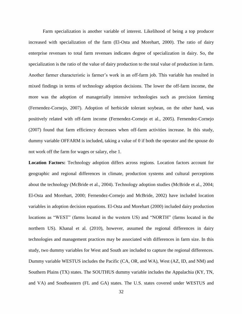
study, two dummy variables for West and South are included to capture the regional differences.
Dummy variable WESTUS includes the Pacific (CA, OR, and WA), West (AZ, ID, and NM) and
Southern Plains (TX) states. The SOUTHUS dummy variable includes the Appalachia (KY, TN,
and VA) and Southeastern (FL and GA) states. The U.S. states covered under WESTUS and

33
SOUTHUS in our study is shown in Figure 3.2. Figure 3.2 also shows the base survey states not
included under WESTUS and SOUTHUS.
Figure 3.2: Survey States Included Under WESTUS and SOUTHUS
Adoption of Other Technologies and Management Practices: According to Johnson and
Ruttan (1997), “..an understanding of principles of breeding and genetics, as well as performance
data collection, management and analysis, are often necessary in order to use the new breeding
technology effectively.” This implies that the adoption of some other technology or milk
production system or management practices may be complementary with breeding technologies.
So, adoption of some particular technologies, management practices or production systems can
influence the adoption decision of breeding technologies. Studies related to the adoption of dairy
technologies (McBride et al., 2004; Foltz and Chang, 2002) have found differences in the
probability of adoption when accounting for other technologies in the adoption equation. Khanal
et al. (2010) have found complementary relationships between dairy technologies, management
practices and/or production systems. Their study found that having a parlor milking system on
34
the farm was the most common factor that increased the likelihood of adoption of most of the
other technologies, management practices and production systems on dairy farms. We include
dummy variable, PARLOR, having value =1 if it is adopted on the farm.
3.2.2 Farm Impact Model
3.2.2.1 Model Set-up
A farm impact model assesses the impact of the adoption of breeding technologies (AI
and ET and/or sexed semen) on farm productivity and farm profitability. Milk production per
cow is used as an indicator of farm productivity while net returns variables are used as indicators
of farm profitability.
If Yi is the productivity or profitability of the farm, expressed in terms of dollars or
amount milk produced, then it is a function of vectors of explanatory variables (Xi) and two
dummy variables for adoption of breeding technologies (AI and ETSS), ETSS being a dummy
variable having value =1 if ET and/or sexed semen is adopted.
where is the vector of parameters for independent variables other than AI and ETSS, AI and
ETSS are two dummy variables having value 1 for adoption and 0 for non-adoption, with 1 and
2 as respective parameters. Estimate ei is the random error term.
From the previous discussions on the adoption decision model, we know that farmers will
adopt each technology if the benefit associated with adoption is higher than the cost associated
with adopting. Let AI* and ETSS* be unknown variables denoting this benefit factor. AI* and
ETSS* depend on several variables (say, whose vectors are βa and βb) such that
ETSS*= X1βa + ε1 and AI*= X2βb + ε2. Then, ETSS =1 if ETSS* > 0 and AI= 1 if AI* > 0.

35
Other technologies adopted on the farm also have the influence on productivity and profitability.
So, if is a vector of other technologies, management practices, and production systems on the
farm, we can rewrite our model as:
, where is the coefficient vector.
3.2.2.2 Accounting for Endogeneity and Self-Selection Bias Issues
The above mentioned equation can be estimated using the Ordinary Least Squares (OLS)
regression technique. However, the estimators computed using a simple OLS technique may be
biased and inconsistent if there is a problem of the presence of the correlation between the
explanatory variables and error terms. If there is potential for such a problem, it should be tested
and corrected for to reduce bias and obtain a more consistent approximation of the estimator.
Explanatory variables which have such correlation with the error term are said to be
endogenous and the least squares estimator fails to estimate accurately in this case (Hill et al.,
2008). We suspect that AI and ETSS are endogenous. This problem can be addressed by
administration of appropriate instrumental variables.
Hill et al. (2008) have explained that the endogeneity problem may arise due to one or
more of the following reasons: 1) measurement problems (the explanatory variable is measured
with error), 2) the case where an omitted variable is correlated with explanatory variables, then
resulting in the error term being correlated with explanatory variables, 3) simultaneous equation
bias, and 4) when a lagged dependent variable is in the model (due to serial correlation).
Any of the reasons mentioned above may cause endogeneity. In our study, there is a need
to test for potential endogeneity of ETSS and AI in impact (profit, revenue, and cost) equations.
If endogeneity is detected, ETSS and AI should be replaced with appropriate instrumental
variables (Greene, 2008). Several previous studies (Foltz and Chang, 2002; Fernandez-Cornejo
et al., 2002; Fernandez-Cornejo and McBride, 2002) have used predicted probabilities from the
36
adoption decision model (probit equation) as instrumental variables in a profit equation. Foltz
and Chang (2002) showed that the probability of adoption can serve as an instrument for
adoption of that technology (in their study, the case was rbST adoption). El-Osta et al. (2007)
used predicted probabilities as instruments in a multinomial regression model.
Note that AI and ETSS decisions are related to each other as described in the adoption
decision model. So, to account for the endogeneity, if detected, predicted probabilities from a
bivariate probit model can be used as instruments in the productivity/ profitability equations to
account for joint probability of adoption. So, after replacing AI and ETSS variables with their
predicted probabilities, our equation would be:
, where and
are the predicted probabilities.
Self selection could be an issue here. We have not assigned farmers as adopters and non-
adopters; they have chosen themselves to be adopters / non-adopters. Thus, the two categories of
farmers as adopters and non-adopters may be systematically different, leading to differences in farm
performance, but that difference may not be solely due to the adoption of technology of interest
(Greene, 2002; Fernendez-Cornejo and McBride 2002). If we ignore self-selection bias in
estimating the impact, then this equation would lead to inconsistent estimates. Since larger farms
are more likely to adopt many advanced technologies, management practices or production systems,
the impact of a particular one on farm profitability and productivity may be biased unless accounted
for using the impact of others using selection bias correction (Khanal et al., 2010).
Selection-bias can be corrected for using self-selection variables in the impact estimation
equation. Heckman‟s (1979) procedure is applicable. This involves computing self-selection
variables from the adoption decision model and then placing them in the impact model. From the
bivariate probit with selection equation in the adoption decision model, selection terms, or the
inverse Mill ratios (λ), are calculated and used as variables in the productivity/ profitability
37
equations. We obtain two selection variables ( and ) from the bivariate probit model for AI and
ET, respectively.
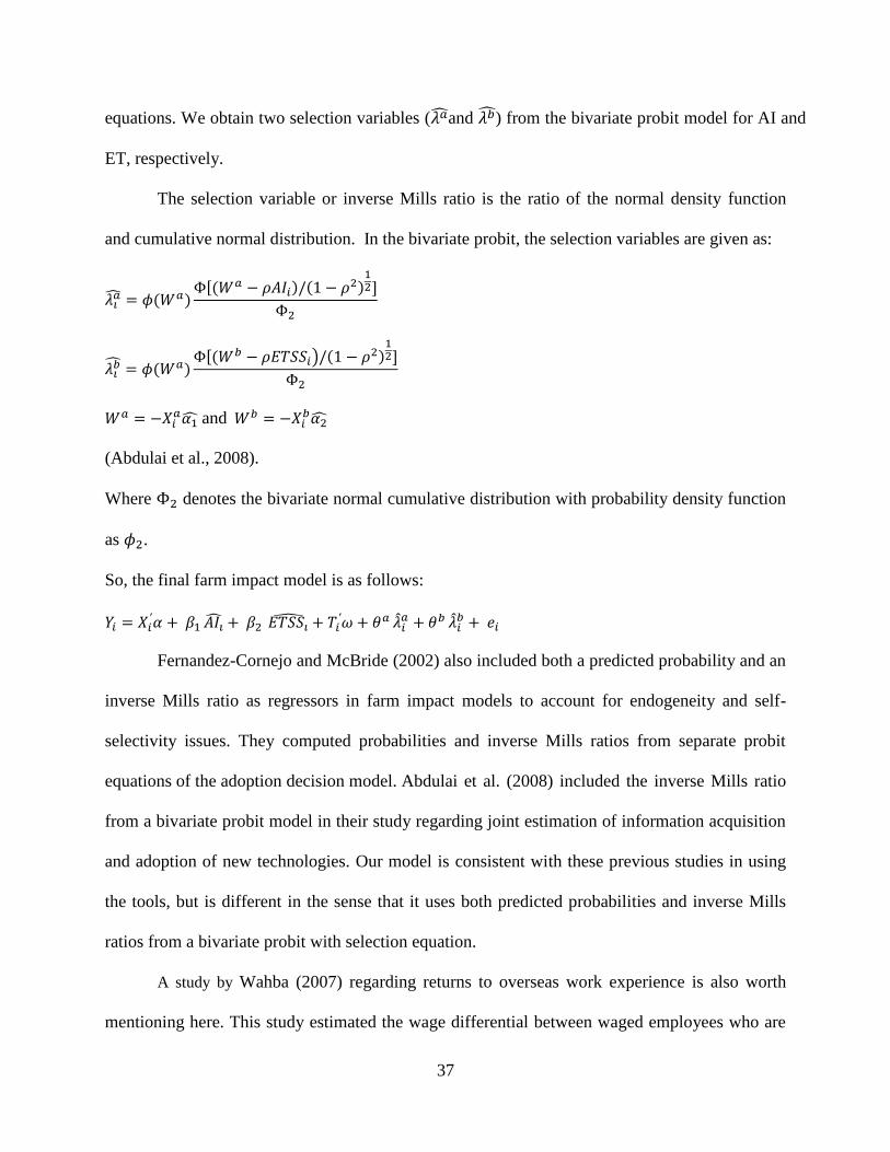
The selection variable or inverse Mills ratio is the ratio of the normal density function
and cumulative normal distribution. In the bivariate probit, the selection variables are given as:
and
(Abdulai et al., 2008).
Where denotes the bivariate normal cumulative distribution with probability density function
as .
So, the final farm impact model is as follows:
Fernandez-Cornejo and McBride (2002) also included both a predicted probability and an
inverse Mills ratio as regressors in farm impact models to account for endogeneity and self-
selectivity issues. They computed probabilities and inverse Mills ratios from separate probit
equations of the adoption decision model. Abdulai et al. (2008) included the inverse Mills ratio
from a bivariate probit model in their study regarding joint estimation of information acquisition
and adoption of new technologies. Our model is consistent with these previous studies in using
the tools, but is different in the sense that it uses both predicted probabilities and inverse Mills
ratios from a bivariate probit with selection equation.
A study by Wahba (2007) regarding returns to overseas work experience is also worth
mentioning here. This study estimated the wage differential between waged employees who are
38
return migrants and those who are non-migrants. Two potential selection biases due to the
migration decision and wage employment participation (labor market participation) were taken
into account. The study regarded Egypt, where purpose of migration was employment and
temporary overseas work experience was affecting wages. Wahba mentioned that there may be
two potential selection biases: one is migration selection bias because migrated returnees may
not be representatives of a random sample, but are self-selected. The second bias in selection
could be on wage work as returnees have alternatives of not entering the wage market, e.g., being
self-employed). To handle this situation, Wahba used a two-step Heckman (1979) approach but
with extended correction terms. In the first step, two selection equations are jointly estimated
using maximum likelihood bivariate probit with selection. In the second stage, the wage
equations were estimated through simple OLS including the correction terms (computed from
bivariate probit results) as additional regressors.
3.2.2.3 Test for Endogeneity and Overidentifying Restrictions
To check whether predicted probabilities of AI and ETSS from adoption decisions are
appropriate versus the actual values for AI and ETSS, we tested for the significance of predicted
values for AI and ETSS, PredAI and PredETSS, respectively in a multiple regression with all Xs,
AI, ET and PredAI and PredETSS as regressors. Since in our case, joint significance of AI and
ETSS was found, we included both the predicted values of AI and ETSS (i.e. PredAI and
PredETSS) in model estimation when either was significant. If not, we chose AI and ETSS
instead of their predicted values. This procedure is based on suggestions by Wooldridge (2006)
for testing endogeneity and overidentifying restrictions, whose general procedure is as follows:
Estimate the reduced form equation for the suspected endogenous variable and obtain the
residual of the equation as
39
Add as an independent variable in the structural equation which also includes the
suspected endogenous variable as an independent variable.
Regress the equation and check for the significance of . If , in the structural equation,
is statistically different from zero, we conclude that the suspected variable is indeed
endogenous.
If endogeneity was detected following this procedure, we included predicted values in
structural equations. After choosing predicted or actual ones from the above mentioned
procedure, we also included λ1 and λ2 (self-selection variables) as exogenous regressors and
checked for their significance. We dropped those in the structural equation if neither were
significantly different from zero while both λ1 and λ2 were included if either was significant.
3.2.2.4 Heteroskedasticity Correction in the Model
We say that heteroskedasticity is present when a sequence of random variables has
different variances. This violates the assumption of equal variances in least squares estimation. If
there is heteroskedasticity, OLS estimators remain unbiased and consistent, but are inefficient.
So, OLS will be no longer result in the BLUE (Best Linear Unbiased Estimator).
There are several procedures to correct for heteroskedasticity. We can stabilize the
variances by transformation of the dependent variables. If there is a prior expectation about the
form of heteroskedasticity, we can use a Generalized (or weighted) least squares estimator
instead of OLS. If there is suspicion of the presence of heteroskedasticity, but we are unaware of
the type of heteroskedasticity, then HCCM (Heteroskedasticity Consistent Covariance Matrix)
estimators are used to obtain more efficient standard errors of the OLS estimates (Long and
Ervin, 2000). Long and Ervin (2000) studied different methods of HCCM, suggesting that if the
number of observations is less than 250, HC3 (HCCM estimator based on hat matrix) would
40
perform better. They suggested that if the sample size is more than 500, any HCCM-based test
(White, HC1, HC2, and HC3) performs well.
As a robust covariance matrix, the White estimator is one of the common estimators,
which is:
(LIMDEP, version 9)
To account for the heteroskedasticity in the impact equations, we used the “Heteroscedasticity”
option that corrects heteroskedasticity through the corrected White estimator (LIMDEP, version
9).
3.2.2.5 Variables in Farm Impact Models
Dependent Variables
Dependent variables in the impact models are variables accounting for farm productivity,
profitability, cost, and revenues. Dairy enterprise net returns over total costs are included as the
indication of farm profitability while milk per cow is the indication of farm productivity. The
gross return (revenue) and the total and allocated cost variables are also used as dependent
variables.
Dairy enterprise net returns are the difference between gross returns and total costs. Gross
returns include the value of milk sold, revenues from sales of culled cattle, the implicit fertilizer
value of manure produced, and other income from the dairy. Operating costs include feed
(including the implicit value of homegrown feed), veterinary and medical, bedding, marketing,
custom services, fuel, lube, electricity, repairs, other operating costs and interest on operating
costs. Allocated overhead costs include: hired labor, the opportunity cost of unpaid labor, capital
recovery of machinery and equipment, the opportunity cost of land (rental rate), taxes and
insurance, and general farm overhead. Each of the following variables is used in a separate
equation as a dependent variable to assess impact.
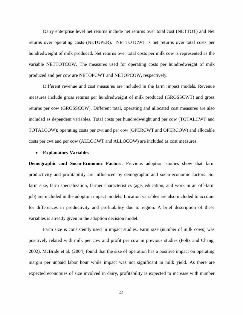
41
Dairy enterprise level net returns include net returns over total cost (NETTOT) and Net
returns over operating costs (NETOPER). NETTOTCWT is net returns over total costs per
hundredweight of milk produced. Net returns over total costs per milk cow is represented as the
variable NETTOTCOW. The measures used for operating costs per hundredweight of milk
produced and per cow are NETOPCWT and NETOPCOW, respectively.
Different revenue and cost measures are included in the farm impact models. Revenue
measures include gross returns per hundredweight of milk produced (GROSSCWT) and gross
returns per cow (GROSSCOW). Different total, operating and allocated cost measures are also
included as dependent variables. Total costs per hundredweight and per cow (TOTALCWT and
TOTALCOW); operating costs per cwt and per cow (OPERCWT and OPERCOW) and allocable
costs per cwt and per cow (ALLOCWT and ALLOCOW) are included as cost measures.
Explanatory Variables
Demographic and Socio-Economic Factors: Previous adoption studies show that farm
productivity and profitability are influenced by demographic and socio-economic factors. So,
farm size, farm specialization, farmer characteristics (age, education, and work in an off-farm
job) are included in the adoption impact models. Location variables are also included to account
for differences in productivity and profitability due to region. A brief description of these
variables is already given in the adoption decision model.
Farm size is consistently used in impact studies. Farm size (number of milk cows) was
positively related with milk per cow and profit per cow in previous studies (Foltz and Chang,
2002). McBride et al. (2004) found that the size of operation has a positive impact on operating
margin per unpaid labor hour while impact was not significant in milk yield. As there are
expected economies of size involved in dairy, profitability is expected to increase with number
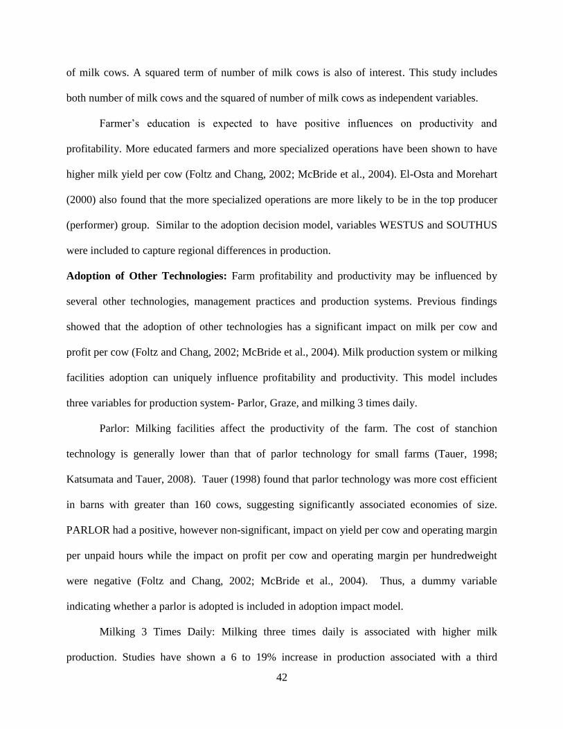
42
of milk cows. A squared term of number of milk cows is also of interest. This study includes
both number of milk cows and the squared of number of milk cows as independent variables.
Farmer‟s education is expected to have positive influences on productivity and
profitability. More educated farmers and more specialized operations have been shown to have
higher milk yield per cow (Foltz and Chang, 2002; McBride et al., 2004). El-Osta and Morehart
(2000) also found that the more specialized operations are more likely to be in the top producer
(performer) group. Similar to the adoption decision model, variables WESTUS and SOUTHUS
were included to capture regional differences in production.
Adoption of Other Technologies: Farm profitability and productivity may be influenced by
several other technologies, management practices and production systems. Previous findings
showed that the adoption of other technologies has a significant impact on milk per cow and
profit per cow (Foltz and Chang, 2002; McBride et al., 2004). Milk production system or milking
facilities adoption can uniquely influence profitability and productivity. This model includes
three variables for production system- Parlor, Graze, and milking 3 times daily.
Parlor: Milking facilities affect the productivity of the farm. The cost of stanchion
technology is generally lower than that of parlor technology for small farms (Tauer, 1998;
Katsumata and Tauer, 2008). Tauer (1998) found that parlor technology was more cost efficient
in barns with greater than 160 cows, suggesting significantly associated economies of size.
PARLOR had a positive, however non-significant, impact on yield per cow and operating margin
per unpaid hours while the impact on profit per cow and operating margin per hundredweight
were negative (Foltz and Chang, 2002; McBride et al., 2004). Thus, a dummy variable
indicating whether a parlor is adopted is included in adoption impact model.
Milking 3 Times Daily: Milking three times daily is associated with higher milk
production. Studies have shown a 6 to 19% increase in production associated with a third
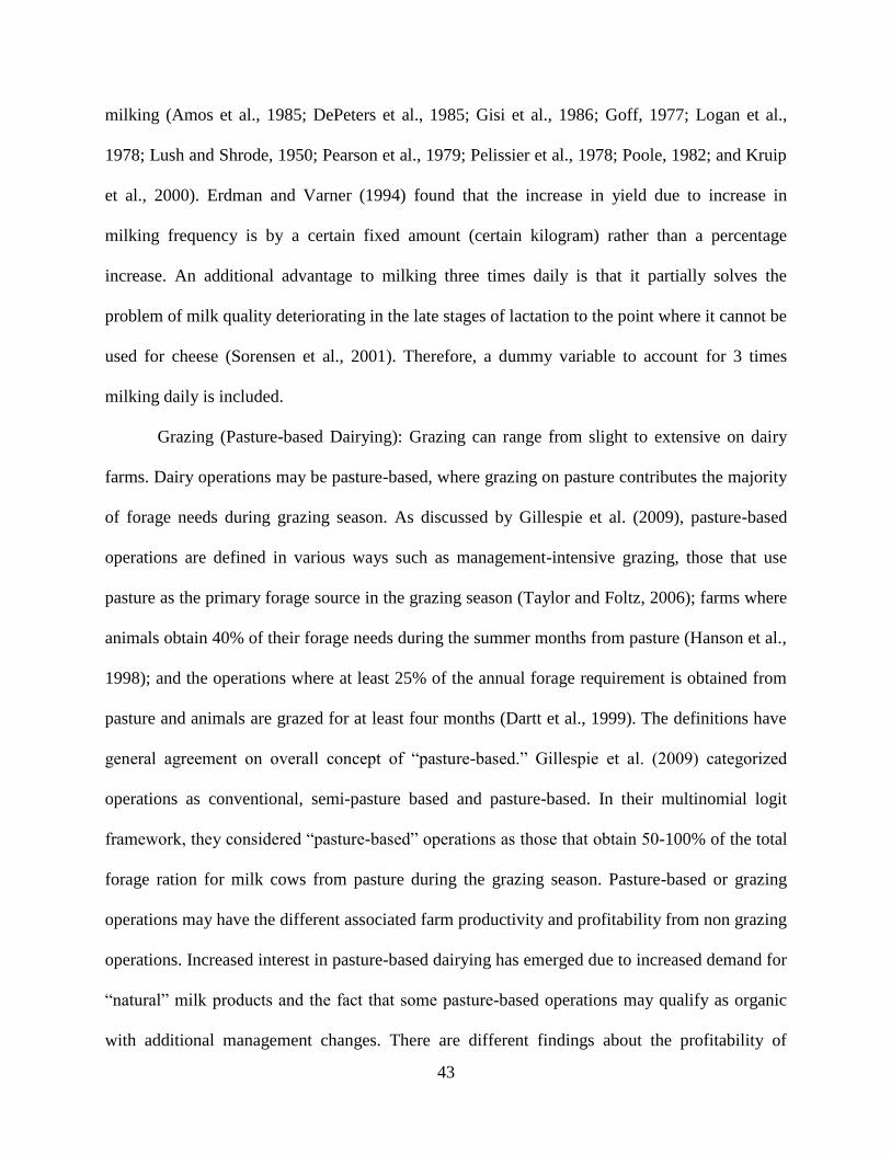
43
milking (Amos et al., 1985; DePeters et al., 1985; Gisi et al., 1986; Goff, 1977; Logan et al.,
1978; Lush and Shrode, 1950; Pearson et al., 1979; Pelissier et al., 1978; Poole, 1982; and Kruip
et al., 2000). Erdman and Varner (1994) found that the increase in yield due to increase in
milking frequency is by a certain fixed amount (certain kilogram) rather than a percentage
increase. An additional advantage to milking three times daily is that it partially solves the
problem of milk quality deteriorating in the late stages of lactation to the point where it cannot be
used for cheese (Sorensen et al., 2001). Therefore, a dummy variable to account for 3 times
milking daily is included.
Grazing (Pasture-based Dairying): Grazing can range from slight to extensive on dairy
farms. Dairy operations may be pasture-based, where grazing on pasture contributes the majority
of forage needs during grazing season. As discussed by Gillespie et al. (2009), pasture-based
operations are defined in various ways such as management-intensive grazing, those that use
pasture as the primary forage source in the grazing season (Taylor and Foltz, 2006); farms where
animals obtain 40% of their forage needs during the summer months from pasture (Hanson et al.,
1998); and the operations where at least 25% of the annual forage requirement is obtained from
pasture and animals are grazed for at least four months (Dartt et al., 1999). The definitions have
general agreement on overall concept of “pasture-based.” Gillespie et al. (2009) categorized
operations as conventional, semi-pasture based and pasture-based. In their multinomial logit
framework, they considered “pasture-based” operations as those that obtain 50-100% of the total
forage ration for milk cows from pasture during the grazing season. Pasture-based or grazing
operations may have the different associated farm productivity and profitability from non grazing
operations. Increased interest in pasture-based dairying has emerged due to increased demand for
“natural” milk products and the fact that some pasture-based operations may qualify as organic
with additional management changes. There are different findings about the profitability of
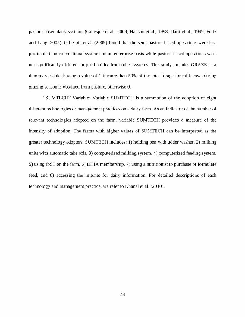
44
pasture-based dairy systems (Gillespie et al., 2009; Hanson et al., 1998; Dartt et al., 1999; Foltz
and Lang, 2005). Gillespie et al. (2009) found that the semi-pasture based operations were less
profitable than conventional systems on an enterprise basis while pasture-based operations were
not significantly different in profitability from other systems. This study includes GRAZE as a
dummy variable, having a value of 1 if more than 50% of the total forage for milk cows during
grazing season is obtained from pasture, otherwise 0.
“SUMTECH” Variable: Variable SUMTECH is a summation of the adoption of eight
different technologies or management practices on a dairy farm. As an indicator of the number of
relevant technologies adopted on the farm, variable SUMTECH provides a measure of the
intensity of adoption. The farms with higher values of SUMTECH can be interpreted as the
greater technology adopters. SUMTECH includes: 1) holding pen with udder washer, 2) milking
units with automatic take offs, 3) computerized milking system, 4) computerized feeding system,
5) using rbST on the farm, 6) DHIA membership, 7) using a nutritionist to purchase or formulate
feed, and 8) accessing the internet for dairy information. For detailed descriptions of each
technology and management practice, we refer to Khanal et al. (2010).

45
CHAPTER 4
RESULTS AND DISCUSSION
The results of adoption decision models and farm impact models developed in Chapter 3
are presented in this chapter. First, the breeding technology adopter characteristics are presented.
Demographic, socio-economic, and financial characteristics of the adopters and non-adopters are
compared. Then, results of the adoption decision and farm impact models are presented and
discussed. The adoption decision model includes the results of separate probits and a bivariate
probit with selection. The farm impact models show the least squares regression results,
accounting for endogeneity and self-selection bias wherever necessary. Each data unit (farm)
used in these analyses is weighted on the basis of the weights assigned in ARMS and are
corrected for potential heteroskedasticity. The econometric software LIMDEP, version 9, was
used for analysis.
4.1 Characteristics of Adopters and Non-Adopters
Adopter and non-adopter differences across various demographic, socioeconomic, and farm
financial characteristics are presented in Table 4.1. Mean differences of the adopters and non-
adopters are statistically tested using paired t-tests. These results are based on 1,814 observations
of ARMS 2005 data employing pair-wise two-tailed delete-a-group Jackknife t-statistics at the
90% confidence level or more. There were 15 replicates and 28 degrees of freedom using the
jackknife. For greater detail on this estimation procedure using ARMS, the reader is referred to
Dubman (2000). The null hypothesis in two-tailed paired t-tests was B1=B2=0, where B1 and B2
are respective variable means of adopters and non-adopters.
Our results presented in Table 4.1 shows the characteristics of adopters and non-adopters.
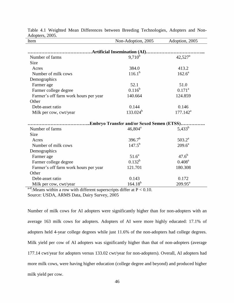
46
Table 4.1 Weighted Mean Differences between Breeding Technologies, Adopters and Non-
Adopters, 2005.
Item Non-Adoption, 2005 Adoption, 2005
……………………………………Artificial Insemination (AI)………………………………...
Number of farms 9,710b
42,527a
Size
Acres 384.0 413.2
Number of milk cows 116.1b
162.6a
Demographics
Farmer age 52.1 51.0
Farmer college degree 0.116b
0.171a
Farmer‟s off farm work hours per year 140.664 124.859
Other
Debt-asset ratio 0.144 0.146
Milk per cow, cwt/year 133.024b
177.142a
…………………………………..Embryo Transfer and/or Sexed Semen (ETSS)…………….
Number of farms 46,804a
5,433b
Size
Acres 396.7b
503.2a
Number of milk cows 147.5b
209.6a
Demographics
Farmer age 51.6a
47.6b
Farmer college degree 0.132b
0.408a
Farmer‟s off farm work hours per year 121.701 180.308
Other
Debt-asset ratio 0.143 0.172
Milk per cow, cwt/year 164.18b
209.95a
a-d:Means within a row with different superscripts differ at P < 0.10.
Source: USDA, ARMS Data, Dairy Survey, 2005
Number of milk cows for AI adopters were significantly higher than for non-adopters with an
average 163 milk cows for adopters. Adopters of AI were more highly educated: 17.1% of
adopters held 4-year college degrees while just 11.6% of the non-adopters had college degrees.
Milk yield per cow of AI adopters was significantly higher than that of non-adopters (average
177.14 cwt/year for adopters versus 133.02 cwt/year for non-adopters). Overall, AI adopters had
more milk cows, were having higher education (college degree and beyond) and produced higher
milk yield per cow.
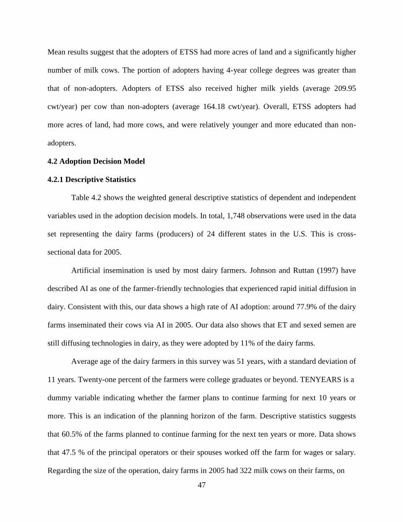
47
Mean results suggest that the adopters of ETSS had more acres of land and a significantly higher
number of milk cows. The portion of adopters having 4-year college degrees was greater than
that of non-adopters. Adopters of ETSS also received higher milk yields (average 209.95
cwt/year) per cow than non-adopters (average 164.18 cwt/year). Overall, ETSS adopters had
more acres of land, had more cows, and were relatively younger and more educated than non-
adopters.
4.2 Adoption Decision Model
4.2.1 Descriptive Statistics
Table 4.2 shows the weighted general descriptive statistics of dependent and independent
variables used in the adoption decision models. In total, 1,748 observations were used in the data
set representing the dairy farms (producers) of 24 different states in the U.S. This is cross-
sectional data for 2005.
Artificial insemination is used by most dairy farmers. Johnson and Ruttan (1997) have
described AI as one of the farmer-friendly technologies that experienced rapid initial diffusion in
dairy. Consistent with this, our data shows a high rate of AI adoption: around 77.9% of the dairy
farms inseminated their cows via AI in 2005. Our data also shows that ET and sexed semen are
still diffusing technologies in dairy, as they were adopted by 11% of the dairy farms.
Average age of the dairy farmers in this survey was 51 years, with a standard deviation of
11 years. Twenty-one percent of the farmers were college graduates or beyond. TENYEARS is a
dummy variable indicating whether the farmer plans to continue farming for next 10 years or
more. This is an indication of the planning horizon of the farm. Descriptive statistics suggests
that 60.5% of the farms planned to continue farming for the next ten years or more. Data shows
that 47.5 % of the principal operators or their spouses worked off the farm for wages or salary.
Regarding the size of the operation, dairy farms in 2005 had 322 milk cows on their farms, on
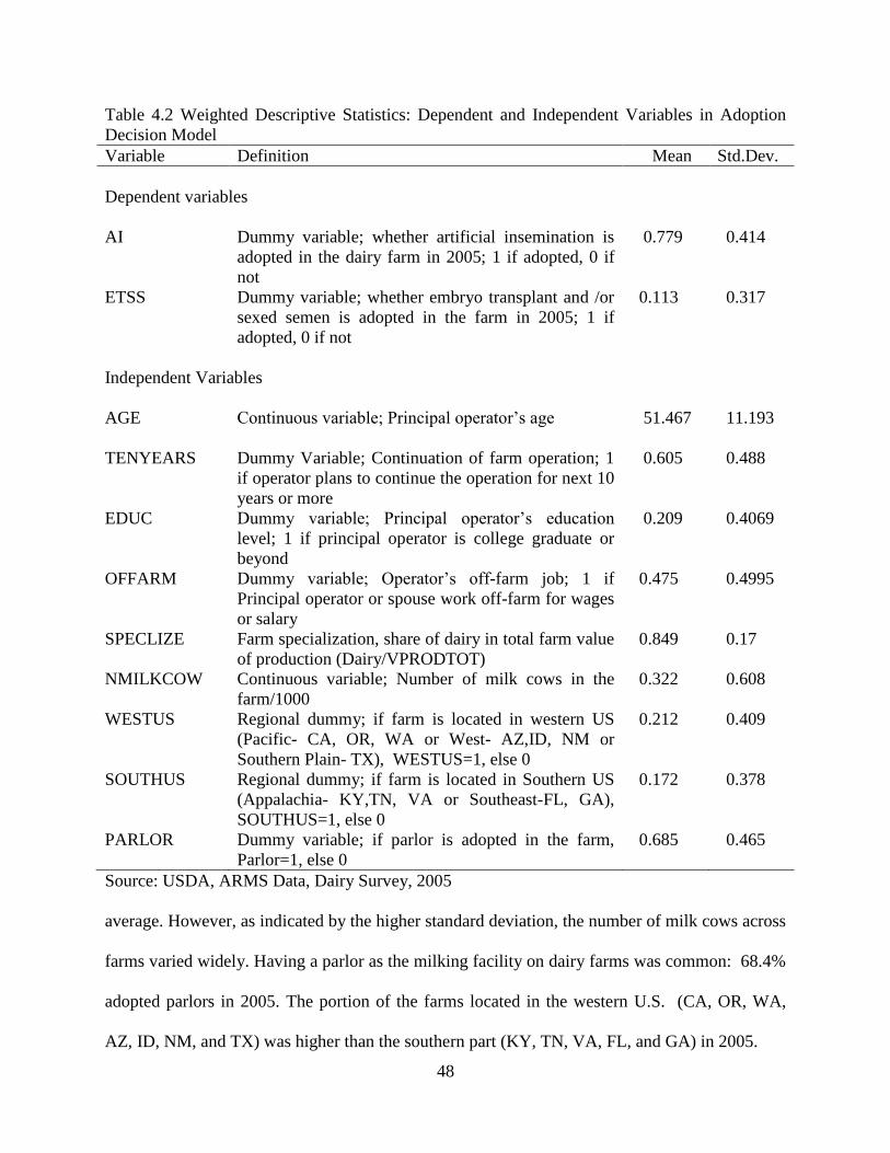
48
Table 4.2 Weighted Descriptive Statistics: Dependent and Independent Variables in Adoption
Decision Model
Source: USDA, ARMS Data, Dairy Survey, 2005
average. However, as indicated by the higher standard deviation, the number of milk cows across
farms varied widely. Having a parlor as the milking facility on dairy farms was common: 68.4%
adopted parlors in 2005. The portion of the farms located in the western U.S. (CA, OR, WA,
AZ, ID, NM, and TX) was higher than the southern part (KY, TN, VA, FL, and GA) in 2005.
Variable Definition Mean Std.Dev.
Dependent variables
AI Dummy variable; whether artificial insemination is
adopted in the dairy farm in 2005; 1 if adopted, 0 if
not
0.779 0.414
ETSS Dummy variable; whether embryo transplant and /or
sexed semen is adopted in the farm in 2005; 1 if
adopted, 0 if not
0.113 0.317
Independent Variables
AGE Continuous variable; Principal operator‟s age 51.467
11.193
TENYEARS Dummy Variable; Continuation of farm operation; 1
if operator plans to continue the operation for next 10
years or more
0.605 0.488
EDUC Dummy variable; Principal operator‟s education
level; 1 if principal operator is college graduate or
beyond
0.209 0.4069
OFFARM Dummy variable; Operator‟s off-farm job; 1 if
Principal operator or spouse work off-farm for wages
or salary
0.475 0.4995
SPECLIZE Farm specialization, share of dairy in total farm value
of production (Dairy/VPRODTOT)
0.849 0.17
NMILKCOW Continuous variable; Number of milk cows in the
farm/1000
0.322 0.608
WESTUS Regional dummy; if farm is located in western US
(Pacific- CA, OR, WA or West- AZ,ID, NM or
Southern Plain- TX), WESTUS=1, else 0
0.212 0.409
SOUTHUS Regional dummy; if farm is located in Southern US
(Appalachia- KY,TN, VA or Southeast-FL, GA),
SOUTHUS=1, else 0
0.172 0.378
PARLOR Dummy variable; if parlor is adopted in the farm,
Parlor=1, else 0
0.685 0.465
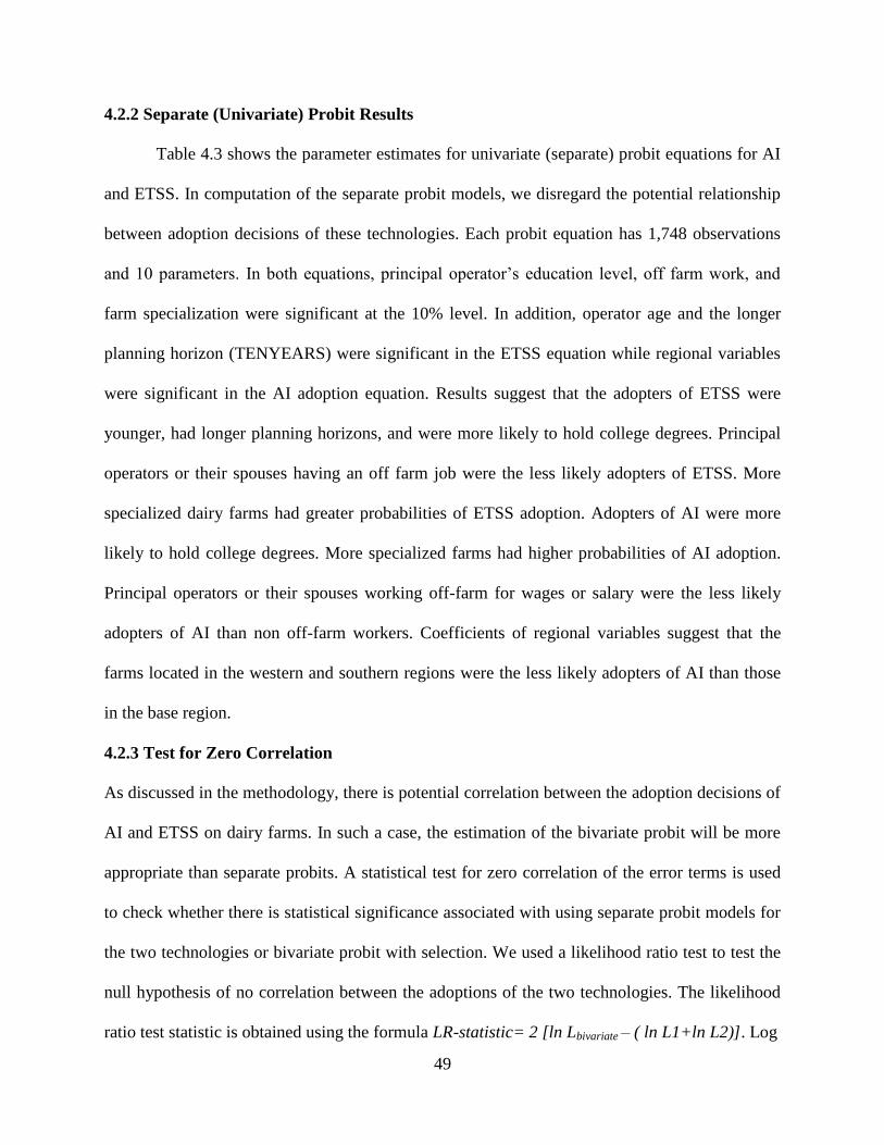
49
4.2.2 Separate (Univariate) Probit Results
Table 4.3 shows the parameter estimates for univariate (separate) probit equations for AI
and ETSS. In computation of the separate probit models, we disregard the potential relationship
between adoption decisions of these technologies. Each probit equation has 1,748 observations
and 10 parameters. In both equations, principal operator‟s education level, off farm work, and
farm specialization were significant at the 10% level. In addition, operator age and the longer
planning horizon (TENYEARS) were significant in the ETSS equation while regional variables
were significant in the AI adoption equation. Results suggest that the adopters of ETSS were
younger, had longer planning horizons, and were more likely to hold college degrees. Principal
operators or their spouses having an off farm job were the less likely adopters of ETSS. More
specialized dairy farms had greater probabilities of ETSS adoption. Adopters of AI were more
likely to hold college degrees. More specialized farms had higher probabilities of AI adoption.
Principal operators or their spouses working off-farm for wages or salary were the less likely
adopters of AI than non off-farm workers. Coefficients of regional variables suggest that the
farms located in the western and southern regions were the less likely adopters of AI than those
in the base region.
4.2.3 Test for Zero Correlation
As discussed in the methodology, there is potential correlation between the adoption decisions of
AI and ETSS on dairy farms. In such a case, the estimation of the bivariate probit will be more
appropriate than separate probits. A statistical test for zero correlation of the error terms is used
to check whether there is statistical significance associated with using separate probit models for
the two technologies or bivariate probit with selection. We used a likelihood ratio test to test the
null hypothesis of no correlation between the adoptions of the two technologies. The likelihood
ratio test statistic is obtained using the formula LR-statistic= 2 [ln Lbivariate – ( ln L1+ln L2)]. Log
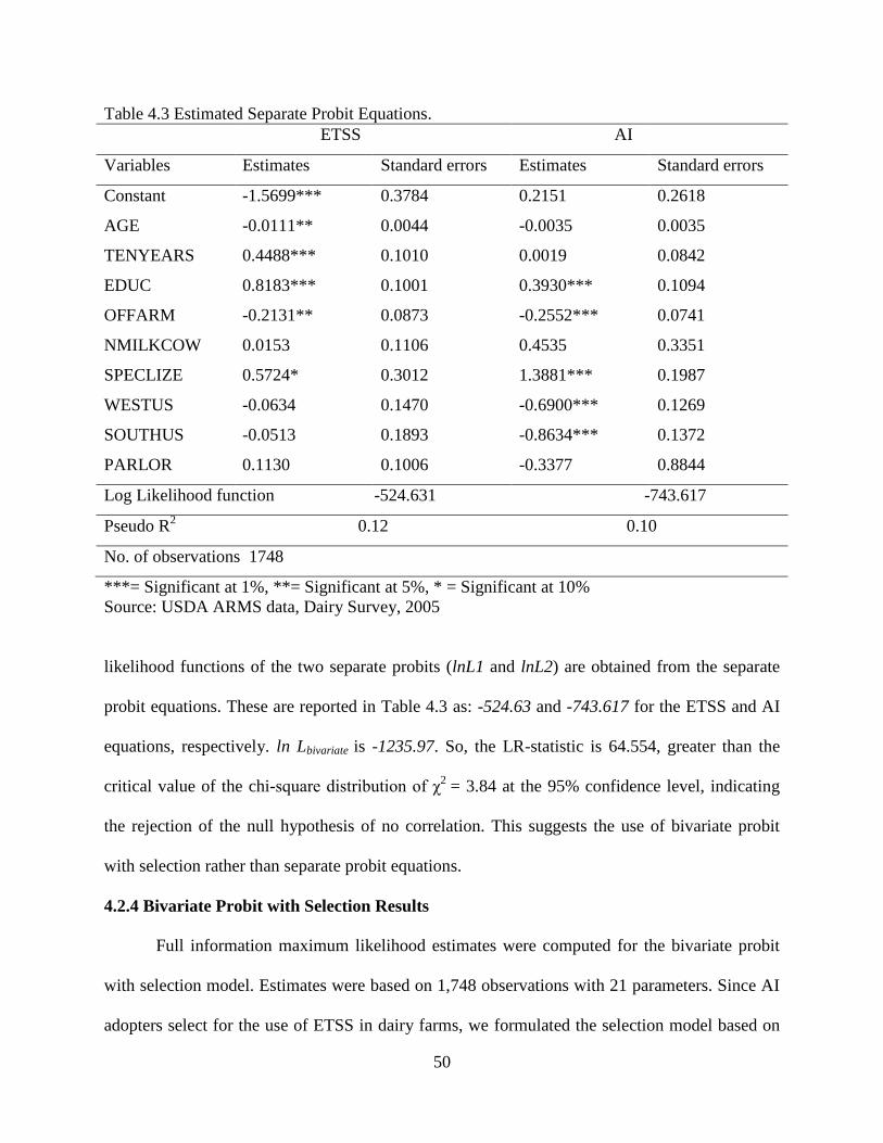
50
Table 4.3 Estimated Separate Probit Equations.
ETSS AI
Variables Estimates Standard errors Estimates Standard errors
Constant -1.5699*** 0.3784 0.2151 0.2618
AGE -0.0111** 0.0044 -0.0035 0.0035
TENYEARS 0.4488*** 0.1010 0.0019 0.0842
EDUC 0.8183*** 0.1001 0.3930*** 0.1094
OFFARM -0.2131** 0.0873 -0.2552*** 0.0741
NMILKCOW 0.0153 0.1106 0.4535 0.3351
SPECLIZE 0.5724* 0.3012 1.3881*** 0.1987
WESTUS -0.0634 0.1470 -0.6900*** 0.1269
SOUTHUS -0.0513 0.1893 -0.8634*** 0.1372
PARLOR 0.1130 0.1006 -0.3377 0.8844
Log Likelihood function -524.631 -743.617
Pseudo R2
0.12 0.10
No. of observations 1748
***= Significant at 1%, **= Significant at 5%, * = Significant at 10%
Source: USDA ARMS data, Dairy Survey, 2005
likelihood functions of the two separate probits (lnL1 and lnL2) are obtained from the separate
probit equations. These are reported in Table 4.3 as: -524.63 and -743.617 for the ETSS and AI
equations, respectively. ln Lbivariate is -1235.97. So, the LR-statistic is 64.554, greater than the
critical value of the chi-square distribution of χ2
= 3.84 at the 95% confidence level, indicating
the rejection of the null hypothesis of no correlation. This suggests the use of bivariate probit
with selection rather than separate probit equations.
4.2.4 Bivariate Probit with Selection Results
Full information maximum likelihood estimates were computed for the bivariate probit
with selection model. Estimates were based on 1,748 observations with 21 parameters. Since AI
adopters select for the use of ETSS in dairy farms, we formulated the selection model based on
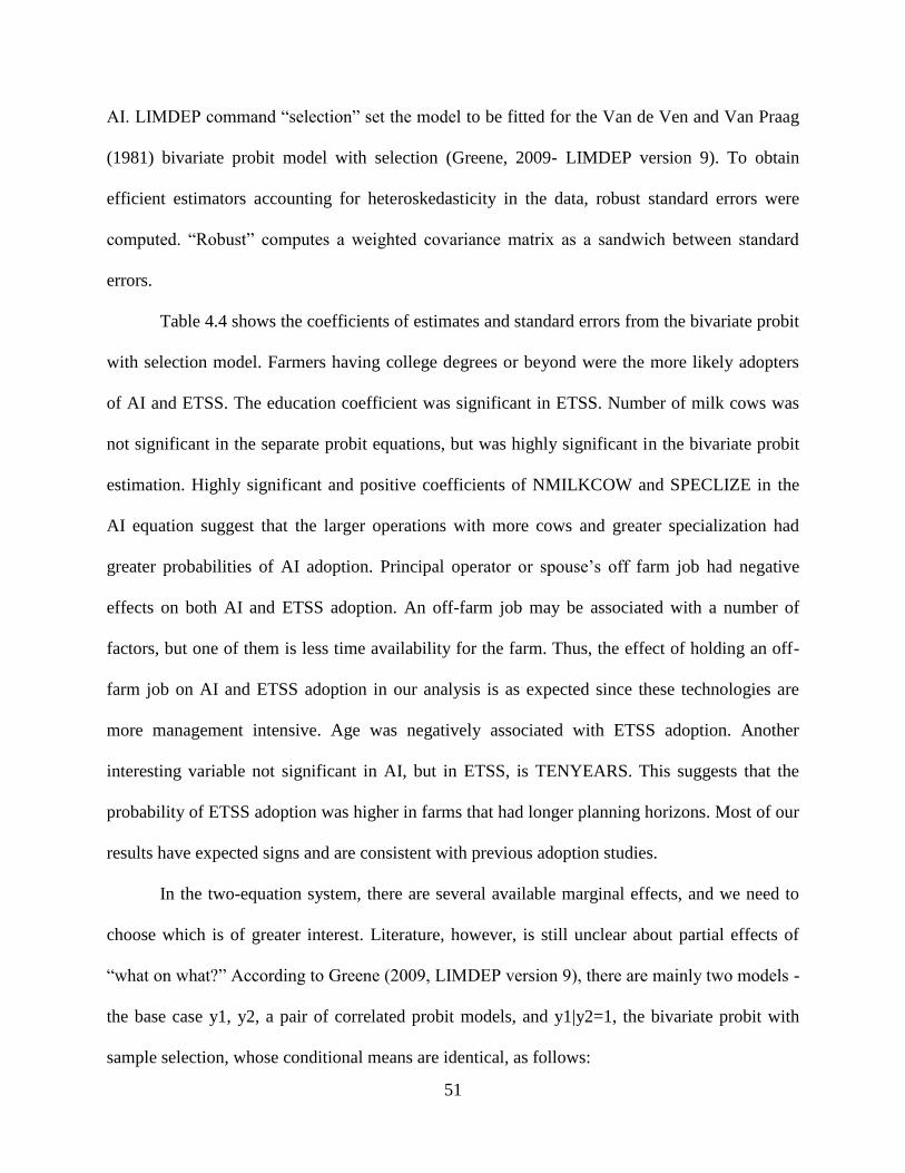
51
AI. LIMDEP command “selection” set the model to be fitted for the Van de Ven and Van Praag
(1981) bivariate probit model with selection (Greene, 2009- LIMDEP version 9). To obtain
efficient estimators accounting for heteroskedasticity in the data, robust standard errors were
computed. “Robust” computes a weighted covariance matrix as a sandwich between standard
errors.
Table 4.4 shows the coefficients of estimates and standard errors from the bivariate probit
with selection model. Farmers having college degrees or beyond were the more likely adopters
of AI and ETSS. The education coefficient was significant in ETSS. Number of milk cows was
not significant in the separate probit equations, but was highly significant in the bivariate probit
estimation. Highly significant and positive coefficients of NMILKCOW and SPECLIZE in the
AI equation suggest that the larger operations with more cows and greater specialization had
greater probabilities of AI adoption. Principal operator or spouse‟s off farm job had negative
effects on both AI and ETSS adoption. An off-farm job may be associated with a number of
factors, but one of them is less time availability for the farm. Thus, the effect of holding an off-
farm job on AI and ETSS adoption in our analysis is as expected since these technologies are
more management intensive. Age was negatively associated with ETSS adoption. Another
interesting variable not significant in AI, but in ETSS, is TENYEARS. This suggests that the
probability of ETSS adoption was higher in farms that had longer planning horizons. Most of our
results have expected signs and are consistent with previous adoption studies.
In the two-equation system, there are several available marginal effects, and we need to
choose which is of greater interest. Literature, however, is still unclear about partial effects of
“what on what?” According to Greene (2009, LIMDEP version 9), there are mainly two models -
the base case y1, y2, a pair of correlated probit models, and y1|y2=1, the bivariate probit with
sample selection, whose conditional means are identical, as follows:
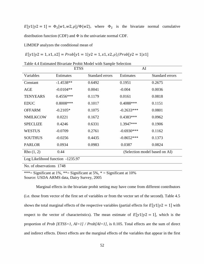
52
, where is the bivariate normal cumulative
distribution function (CDF) and is the univariate normal CDF.
LIMDEP analyzes the conditional mean of
Table 4.4 Estimated Bivariate Probit Model with Sample Selection
ETSS AI
Variables Estimates Standard errors Estimates Standard errors
Constant -1.4538** 0.6492 0.1951 0.2675
AGE -0.0104** 0.0041 -0.004 0.0036
TENYEARS 0.4556*** 0.1179 0.0161 0.0818
EDUC 0.8008*** 0.1017 0.4088*** 0.1151
OFFARM -0.2105* 0.1075 -0.2633*** 0.0801
NMILKCOW 0.0221 0.1672 0.4383*** 0.0962
SPECLIZE 0.4246 0.6331 1.3947*** 0.1906
WESTUS -0.0709 0.2761 -0.6930*** 0.1162
SOUTHUS -0.0256 0.4435 -0.8652*** 0.1373
PARLOR 0.0934 0.0983 0.0387 0.0824
Rho (1, 2) 0.44 (Selection model based on AI)
Log Likelihood function -1235.97
No. of observations 1748
***= Significant at 1%, **= Significant at 5%, * = Significant at 10%
Source: USDA ARMS data, Dairy Survey, 2005
Marginal effects in the bivariate probit setting may have come from different contributors
(i.e. those from vector of the first set of variables or from the vector set of the second). Table 4.5
shows the total marginal effects of the respective variables (partial effects for with
respect to the vector of characteristics). The mean estimate of , which is the
proportion of Prob [ETSS=1, AI=1] / Prob[AI=1], is 0.105. Total effects are the sum of direct
and indirect effects. Direct effects are the marginal effects of the variables that appear in the first
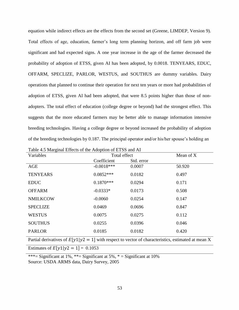
53
equation while indirect effects are the effects from the second set (Greene, LIMDEP, Version 9).
Total effects of age, education, farmer‟s long term planning horizon, and off farm job were
significant and had expected signs. A one year increase in the age of the farmer decreased the
probability of adoption of ETSS, given AI has been adopted, by 0.0018. TENYEARS, EDUC,
OFFARM, SPECLIZE, PARLOR, WESTUS, and SOUTHUS are dummy variables. Dairy
operations that planned to continue their operation for next ten years or more had probabilities of
adoption of ETSS, given AI had been adopted, that were 8.5 points higher than those of non-
adopters. The total effect of education (college degree or beyond) had the strongest effect. This
suggests that the more educated farmers may be better able to manage information intensive
breeding technologies. Having a college degree or beyond increased the probability of adoption
of the breeding technologies by 0.187. The principal operator and/or his/her spouse‟s holding an
Table 4.5 Marginal Effects of the Adoption of ETSS and AI
Variables Total effect Mean of X
Coefficient Std. error
AGE -0.0018*** 0.0007 50.920
TENYEARS 0.0852*** 0.0182 0.497
EDUC 0.1870*** 0.0294 0.171
OFFARM -0.0333* 0.0173 0.508
NMILKCOW -0.0060 0.0254 0.147
SPECLIZE 0.0469 0.0696 0.847
WESTUS 0.0075 0.0275 0.112
SOUTHUS 0.0255 0.0396 0.046
PARLOR 0.0185 0.0182 0.420
Partial derivatives of with respect to vector of characteristics, estimated at mean X
Estimates of = 0.1053
***= Significant at 1%, **= Significant at 5%, * = Significant at 10%
Source: USDA ARMS data, Dairy Survey, 2005
54
off-farm job reduced the probabilities of adoption of breeding technologies of ETSS, given AI
had been adopted, by 0.033.
4.3 Farm Impact Models
4.3.1 Descriptive Statistics
Table 4.6 shows the general descriptive statistics of the dependent variables used in the
farm impact models. Profitability and productivity measures and revenue and cost measures were
used as dependent variables. Net returns over total cost (NETTOT), Net returns over operating
costs (NETOPER), and those in per hundredweight and per cow bases (NETTOTCWT,
NETTOTCOW, NETOPCWT, NETOPCOW) include revenue and expenses associated with the
dairy enterprise. Dairy farmers received total revenue of $17.95 per cwt milk produced with total
cost of 27.87 per cwt milk produced, for a negative net return of $9.92 per cwt of milk produced.
If we examine on a per cow basis, farmers generated revenues of $2,925.48 with total costs of
$4,164.01 involved, for a negative $1238.61 in net returns over total costs per cow. These
negative results over total costs, however, are not surprising because the costs involved here are
economic costs, including fixed costs. Average net returns over operating costs per cwt of milk
produced were $5.02 and per cow were $880.36. Average allocated costs per cwt of milk
produced were $12.93, while on a per cow basis, $2,045.12. Large standard deviations indicate
that there were wide variations in returns and costs across farms.
Table 4.7 shows the descriptive statistics of independent variables used in the impact
models. Average age of the principal operator was 51 years. Twenty one percent of the dairy
farmers (principal operators) of the farm were college graduates or beyond. Approximately 48%
of the farm‟s principal operator and/or his/her spouse worked off the farm for a job or salary.
Number of milk cows on the farm varied widely, with the average number of milk cows of 322.

55
Table 4.6 Weighted Descriptive Statistics of Dependent Variables Used in Impact Model
Variables Definition Mean Std. Dev.
Profitability, productivity and income measures
NETTOT
Net returns over total cost, dollars
-43,128.53
477,959.03
NETOPER Net returns over operating cost, dollars 169,926.8 634,723.25
NRTOTCWT Net returns over total cost per hundredweight of milk produced, dollars -9.92 12.87
NRTOTCOW Net returns over total cost per cow, dollars -1,238.61 1,362.92
NROPCWT Net returns over operating cost per hundredweight of milk produced, dollars 5.02 5.10
NROPCOW Net returns over total cost per cow, dollars 880.36 820.78
MLKPERCOW Milk yield per cow 165.96 52.42
Revenue measures of the farm
GROSSCWT Gross returns per hundredweight of milk produced (Revenues per cwt) 17.95 3.65
GROSSCOW Gross returns per cow (Revenues per cow) 2,925.48 924.46
Cost measures of the farm
TOTALCWT Total costs per hundredweight of milk produced 27.87 13.72
TOTALCOW Total costs per cow 4,164.01 1262.70
OPERCWT Operating cost per hundredweight of milk produced 12.93 4.83
OPERCOW Operating cost per cow 2,045.12 762.48
ALLOCWT Allocated costs per hundredweight of milk produced 14.94 10.66
ALLOCOW Allocated costs per cow 2,118.97 960.14
Source: USDA, ARMS Data, Dairy Survey, 2005
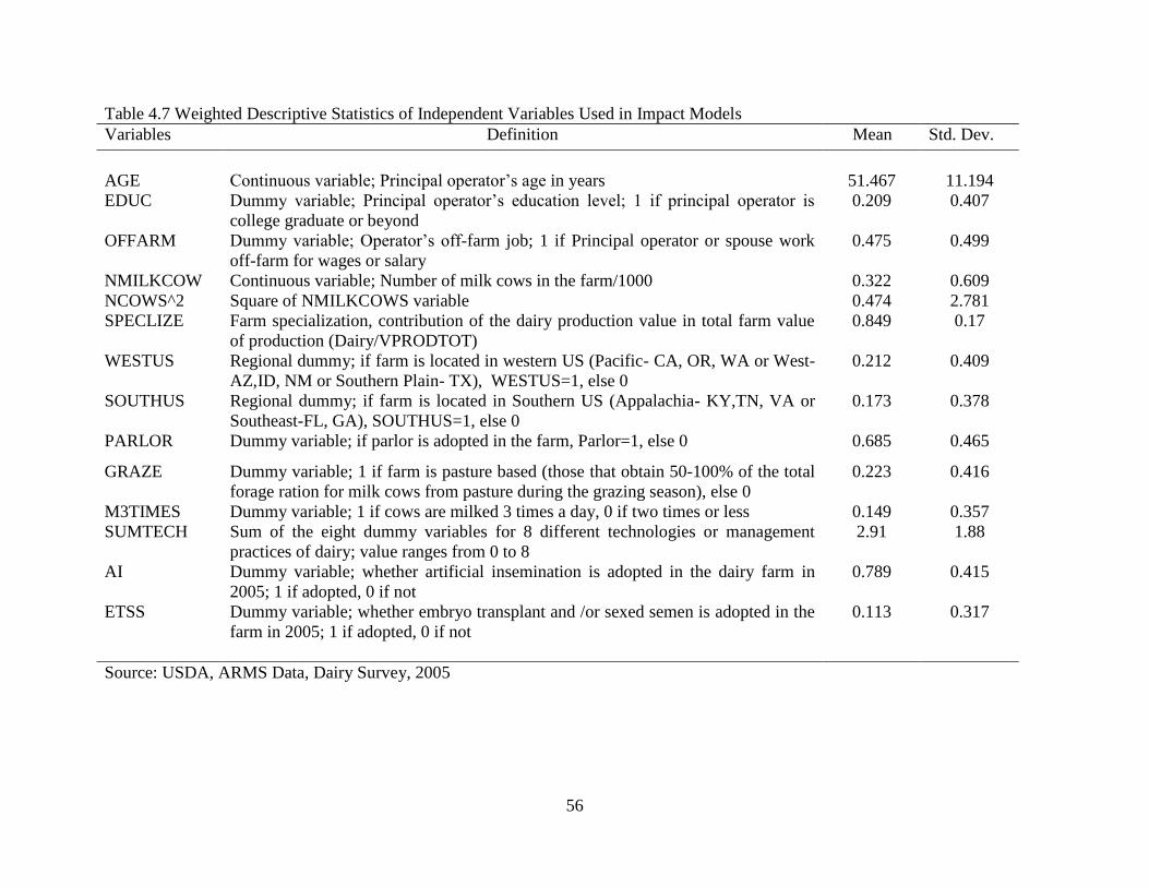
56
Table 4.7 Weighted Descriptive Statistics of Independent Variables Used in Impact Models
Variables Definition Mean Std. Dev.
AGE
Continuous variable; Principal operator‟s age in years
51.467
11.194
EDUC Dummy variable; Principal operator‟s education level; 1 if principal operator is
college graduate or beyond
0.209 0.407
OFFARM
Dummy variable; Operator‟s off-farm job; 1 if Principal operator or spouse work
off-farm for wages or salary
0.475 0.499
NMILKCOW Continuous variable; Number of milk cows in the farm/1000 0.322 0.609
NCOWS^2 Square of NMILKCOWS variable 0.474 2.781
SPECLIZE Farm specialization, contribution of the dairy production value in total farm value
of production (Dairy/VPRODTOT)
0.849 0.17
WESTUS Regional dummy; if farm is located in western US (Pacific- CA, OR, WA or West-
AZ,ID, NM or Southern Plain- TX), WESTUS=1, else 0
0.212 0.409
SOUTHUS Regional dummy; if farm is located in Southern US (Appalachia- KY,TN, VA or
Southeast-FL, GA), SOUTHUS=1, else 0
0.173 0.378
PARLOR Dummy variable; if parlor is adopted in the farm, Parlor=1, else 0 0.685 0.465
GRAZE Dummy variable; 1 if farm is pasture based (those that obtain 50-100% of the total
forage ration for milk cows from pasture during the grazing season), else 0
0.223 0.416
M3TIMES Dummy variable; 1 if cows are milked 3 times a day, 0 if two times or less 0.149 0.357
SUMTECH Sum of the eight dummy variables for 8 different technologies or management
practices of dairy; value ranges from 0 to 8
2.91 1.88
AI Dummy variable; whether artificial insemination is adopted in the dairy farm in
2005; 1 if adopted, 0 if not
0.789 0.415
ETSS Dummy variable; whether embryo transplant and /or sexed semen is adopted in the
farm in 2005; 1 if adopted, 0 if not
0.113 0.317
Source: USDA, ARMS Data, Dairy Survey, 2005
57
The specialization variable indicates that an average of 84.9% of the total value of farm
production was contributed by the dairy enterprise in most of the farms.
Technology adoption variables were quite interesting. About two thirds (68.5%) of the
dairy farms used parlors in their operations. Approximately 14.9% of the farms milked 3 times
daily. AI was adopted by 78.9% of the farms while ETSS was adopted by 11.3% of the farms.
Twenty-two percent of the farms were pasture-based (obtained more than 50% of the total forage
requirement from pasture during the grazing season). This varied widely with a standard
deviation of 0.416. The SUMTECH variable indicates that dairy farms, on average, adopted
approximately 3 of 8 technologies and management practices: holding pens with udder washers,
milkers with automatic take-offs, computerized feeding system, computerized milking system,
assessing internet for information, membership with DHIA, recombinant bovine somatotropin
(rbST) and use nutritionist to formulate or purchase feed.
We included two location variables, SOUTHUS and WESTUS to capture the location
differences. Of the total dairy farms, 21.2% of dairy farms were located in WESTUS - Pacific
(CA, OR, WA, AZ, ID, NM, TX), while the SOUTHUS (KY, TN, VA , FL, GA) had 17.3% of
the dairy farms under study.
4.3.2 Farm Impact and Cost Measures
Tables 4.8 through 4.11 show the OLS results of profitability, productivity and cost
measures of the farm.
4.3.2.1 Net Returns over Costs
Table 4.8 shows the parameter estimates of equations for enterprise net returns over total
costs and enterprise net returns over operating costs. Age is significantly negative in the
NETTOT equation. A one year increase in the age of the principal operator was associated with
a decrease in net returns over total costs of $2,794.81. Highly significant result of NMILKCOW
58
indicates that the net returns over total and operating costs increase with herd size. The western
U.S. had both net returns over total costs and net returns over operating costs that were lower
than those of the base region (North Central and Northeast). Significant negative coefficients of
SUMTECH in both net returns equations indicate that the costs involved in adoption of
subsequent technology (among eight) may be higher than the returns, reducing net returns.
Neither AI nor ETSS was significantly different from zero at the 10% level.
4.3.2.2 Milk Yield per Cow
In Table 4.8, the right-most two columns show the parameter estimates and respective
standard errors of the milk yield per cow equation. An adjusted R2
value of 0.39 suggests that
around 39% of the variation in milk yield per cow is explained by the model. Age of the farmer,
education, off-farm job, and farm specialization are significant at the 1% significance level.
Coefficients of grazing, milking 3 times, and sum of the technologies were also highly
significant (at the 1% level). A negative coefficient of education, indicating an annual decrease
in cwt of milk produced per cow by 9.38, was unexpected. Greater opportunities associated with
the college degree may be one of the explanations. The negative coefficients of off farm job and
age suggest that principal operator or spouse‟s off farm job and older age were associated with
lower milk yield. The SPECLIZE coefficient suggests that more specialized dairy farms had
higher milk yield per cow, as expected. Pasture-based dairy operations were getting lower milk
yield per cow than those using conventional dairies. Our results suggest that milking three times
was associated with a higher milk yield of approximately 21 cwt milk produced per cow than 2
times milking. Coefficients of number of milk cows and squared number of milk cows were not
significantly different from zero at the 10% significance level. The positive and highly
significant coefficient of SUMTECH suggests that those farms adopting greater numbers of

59
Table 4.8 Farm Impact: OLS Estimators of Net Returns over Total and Operating Costs, and Milk Yield per Cow
Dep. Variables NETTOT NETOPER MLKPERCOW
Indep. Variables Coefficient Std. Error Coefficient Std. Error Coefficient Std. Error
Constant 59791.20 101990.10 48759.60 87901.30 160.45*** 10.26
AGE -2794.81** 101990.10 -1529.20 1000.22 -0.84*** 0.09
EDUC 38879.80 1247.09 39268.80 30134.03 -9.38*** 3.14
OFFARM 31811.90 42198.80 15782.80 18263.21 -8.15*** 1.98
NMILKCOW 0.103D+07* 23151.50 0.159D+07*** 347546.90 2.21 6.70
NCOWS^2 -58672.70 529970.50 9956.69 107843.50 -0.89 1.11
SPECLIZE -62668.10 185139.60 -33334.60 73611.19 34.99*** 7.80
WESTUS -106456.00* 86015.67 -128221*** 44819.42 -5.31 3.37
SOUTHUS -42322.10 62241.99 -37962.70 25704.09 -4.75 4.63
PARLOR -22223.50 31527.73 23479.60 21605.49 -1.48 2.48
GRAZE 15928.00 26676.31 9685.65 7446.18 -7.49*** 2.74
M3TIMES 16074.00 104922.00 103462 88393.98 20.88*** 4.21
SUMTECH -27712.20** 13813.91 -13338.00** 93336.34 12.11*** 0.81
AI 26718.80 19282.51 25410.60 21152.75
ETSS -45212.40 34891.38 -31952.80 32439.23
PREDAI 1.25 2.09
PREDETSS 14.98*** 5.01
LAMDAA 7.92*** 2.43
LAMDAB 7.91*** 2.10
Model fit Adj. R2 0.27 Adj. R
2 0.72 Adj. R
2 0.39
Model test F [14, 1733] 46 F [14, 1733] 329.3 F [16, 1731] 71.3
***= Significant at 1%, **= Significant at 5%, * = Significant at 10%; D+aa or D-aa: multiply by 10 to +aa or –aa
Source: USDA, ARMS Data, Dairy Survey, 2005
60
technologies and management practices received higher milk yield per cow in 2005. A
significant and positive coefficient of PREDETSS at the 1% level suggests that higher
probabilities of ETSS technology adoption have a positive impact on milk yield per cow. This is
after accounting for endogeneity and potential self selection issues. Significant lamda
coefficients showed that there was self-selection bias associated with the milk yield equation,
which required correction to reduce bias.
4.3.2.3 Net Returns over Cost per Unit of Input and Output
Table 4.9 shows the parameter estimates for net returns over total expenditures per cwt
and cow bases and net returns over operating expenditures per cwt and per cow bases. These
measures are consistently used in several farm impact studies as indicators of farm profitability.
Short (2000) and Short (2004) included these measures as performance characteristics of dairy
farms. Foltz and Chang (2002) used net returns over total costs per cow. McBride et al. (2002)
considered net returns over operating costs per cwt. Gillespie et al. (2009) included net returns
over total costs per cwt and per cow.
Results suggest that the older farmers have lower net returns over total costs for both per
cwt and per cow measures as well as for net returns over operating expenses per cow. A one year
increase in age of the principal operator is associated with lower net returns of 11 cents over total
costs per cwt milk produced, lower net returns over operating costs of $7.92 per cow, and $13
lower net returns over total costs per cow. Furthermore, education had positive and significant
coefficient in all equations except that of returns over total costs per cow. This suggests that
farmers with college degrees or beyond had greater net returns over both total and operating
costs. A college degree was associated with $2.94 more net returns over total costs per cwt and
$4.11 more net returns over operating costs per cwt. Farmers with college degrees received
$186.67 more returns over operating costs than those not having a degree. A principal operator
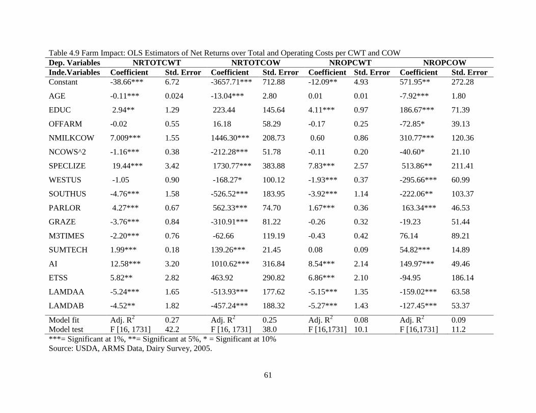
61
Table 4.9 Farm Impact: OLS Estimators of Net Returns over Total and Operating Costs per CWT and COW
Dep. Variables NRTOTCWT NRTOTCOW NROPCWT NROPCOW
Inde.Variables Coefficient Std. Error Coefficient Std. Error Coefficient Std. Error Coefficient Std. Error
Constant -38.66*** 6.72 -3657.71*** 712.88 -12.09** 4.93 571.95** 272.28
AGE -0.11*** 0.024 -13.04*** 2.80 0.01 0.01 -7.92*** 1.80
EDUC 2.94** 1.29 223.44 145.64 4.11*** 0.97 186.67*** 71.39
OFFARM -0.02 0.55 16.18 58.29 -0.17 0.25 -72.85* 39.13
NMILKCOW 7.009*** 1.55 1446.30*** 208.73 0.60 0.86 310.77*** 120.36
NCOWS^2 -1.16*** 0.38 -212.28*** 51.78 -0.11 0.20 -40.60* 21.10
SPECLIZE 19.44*** 3.42 1730.77*** 383.88 7.83*** 2.57 513.86** 211.41
WESTUS -1.05 0.90 -168.27* 100.12 -1.93*** 0.37 -295.66*** 60.99
SOUTHUS -4.76*** 1.58 -526.52*** 183.95 -3.92*** 1.14 -222.06** 103.37
PARLOR 4.27*** 0.67 562.33*** 74.70 1.67*** 0.36 163.34*** 46.53
GRAZE -3.76*** 0.84 -310.91*** 81.22 -0.26 0.32 -19.23 51.44
M3TIMES -2.20*** 0.76 -62.66 119.19 -0.43 0.42 76.14 89.21
SUMTECH 1.99*** 0.18 139.26*** 21.45 0.08 0.09 54.82*** 14.89
AI 12.58*** 3.20 1010.62*** 316.84 8.54*** 2.14 149.97*** 49.46
ETSS 5.82** 2.82 463.92 290.82 6.86*** 2.10 -94.95 186.14
LAMDAA -5.24*** 1.65 -513.93*** 177.62 -5.15*** 1.35 -159.02*** 63.58
LAMDAB -4.52** 1.82 -457.24*** 188.32 -5.27*** 1.43 -127.45*** 53.37
Model fit Adj. R2 0.27 Adj. R
2 0.25 Adj. R
2 0.08 Adj. R
2 0.09
Model test F [16, 1731] 42.2 F [16, 1731] 38.0 F [16,1731] 10.1 F [16,1731] 11.2
***= Significant at 1%, **= Significant at 5%, * = Significant at 10%
Source: USDA, ARMS Data, Dairy Survey, 2005.
62
and/or his/her spouse having off farm job received $72.85 lower net returns over operating costs
per cow than those not having an off-farm job.
Highly significant positive coefficients of number of milk cows indicate that farm size is
positively associated with net returns over total and operating costs on both per cwt and per cow
bases. Coefficients of NCOWS^2 are also significant and negative, suggesting that the maximum
net returns over total costs per cwt were obtained when herd size is around 3,021. Similarly,
increases in numbers of milk cows increase net returns over total costs per cow until the herd
size reaches around 3,400. The peak point to have maximized net returns over operating costs
per cow, on the other hand, was found to be around 3,827. The maximum level of milk cow
number is as suggested by the squared term. Inclusion of the quadratic term places a restriction
of a minimum or maximum level and may not be the actual representation. However, the
quadratic term allows for greater flexibility. Farm specialization is another important factor. Our
Results suggested that the more specialized dairy operations had higher net returns per cow and
per cwt in 2005. If there are significant economies of size associated, then specialization in that
particular enterprise would increase mean financial performance (Purdy et al., 1997). Purdy et al.
(1997) further suggested that the trend of specialization in dairy is likely to continue. Moving
from 100% diversification (0% of income from milk) to 100% specialization resulted in a $19.44
increase in net returns over total costs per cwt and a $7.83 increase in net returns over operating
costs per cwt milk produced. On a per cow basis, the increases were $1,730.77 and $513.86,
respectively. Overall positive impact of specialization on net returns is demonstrated by the
results. Purdy et al. (1997) also found increased financial performance associated with
specialization in dairy. McBride et al. (2004), however, found an unexpected negative coefficient
for specialization in dairy. Overall, signs and coefficients of demographic and farm
characteristics variables in profitability measures in our study are as expected.
63
Farms having parlors were getting higher net returns over total and operating costs on
both per cwt of milk produced and per cow bases. Significant positive impacts included: higher
net returns of $562.33 and $163.34 over total and operating costs, respectively, were shown to be
associated with parlor adoption on per cow bases. On a per cwt milk produced basis, parlor
adopters received additional net returns of $4.27 over total costs and $1.67 over operating costs,
respectively, than non-adopters. Results suggest that the pasture-based dairy operations received
lower net returns over total costs than conventional dairy farms on both per cwt and per cow
bases. Net returns over total costs per cow for pasture-based dairy operations were $310.91 less
than that of non-pasture based. Similarly, pasture based operations experienced lower net returns
of $3.76 over total costs per hundredweight of milk sold. Milking 3 times daily was also negative
and significant in the NRTOTCWT equation, suggesting a decrease of $2.20 in net returns over
total costs on per cwt milk produced basis. Milking 3 times daily was not significant in other
measures. Coefficients of AI were highly significant and positive in all profitability equations in
Table 4.9, indicating a positive impact of the adoption of AI on net returns per cwt milk
produced and per cow. Remarkable increases in net returns over total costs by around $12.58 and
$1,010.62 on per cwt and per cow basis, respectively, were associated with AI adoption. Results
of NROPCWT and NROPCOW equations suggest that AI adopters had $8.54 greater net returns
over operating costs per cwt milk produced than non-adopters, while on a per cow basis, the
measure was $149.97.
Adoption of ETSS was significant and positive in net returns over total and operating
costs per cwt milk produced bases while those on per cow bases were not significant. Results
show that higher net returns of around $5.82 over total costs and around $6.86 over operating
costs, both on per cwt milk produced bases, were associated with ETSS adoption over non-
adoption. Every net return measure on Table 4.9 showed that the adoption of modern dairy
64
technologies (among eight under SUMTECH) was associated with higher profitability.
Significant increases in net returns over total costs by $1.99 and $139.26 were associated with
adoption of each subsequent technology among eight on per cwt of milk produced and per cow
bases, respectively. Similarly, positive net returns of around $54.82 over operating costs per cow
were associated with each subsequent technology adoption.
Highly significant coefficients of lamdas in all profitability equations in Table 4.9 are
particularly noticeable. This suggests that there would have been selection bias present if we had
not accounted and corrected for it. If we had not included selection bias variables (LAMDAA
and LAMDAB) in those regressions, then the estimators of other variables would have biased
coefficients.
4.3.2.4 Gross Returns on the Farm
Gross returns are the total return measures of the dairy enterprise. In 2005, farmers
received $19.23 of gross returns per hundredweight of milk produced and around $3,052.80 per
cow, on average (Table 4.6). Least squares estimates of variables on gross returns per hundred
weight of milk produced and gross returns per cow equations are shown in Table 4.10.
GROSSCWT and GROSSCOW are gross return measures per cwt of milk produced and per cow
bases. Having a college degree or beyond had a significantly positive effect on gross returns per
cwt milk produced. Principal operator‟s age had a negative effect on gross returns per cow. Off-
farm job negatively affected both gross returns (per cwt milk produced and per cow bases)
measures. As farms became more specialized in dairy, they realized lower gross returns per cwt
milk sold than diversified farms in 2005.
Results suggested that having a parlor in the dairy operation was negatively associated
with gross returns. Pasture-based dairies had lower gross returns per cow than conventional. As
indicated by the SUMTECH coefficient, greater technology adopters (adopting a greater number
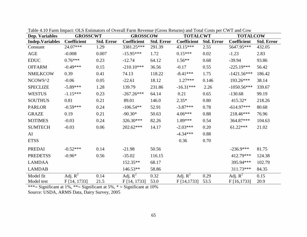
65
Table 4.10 Farm Impact: OLS Estimators of Overall Farm Revenue (Gross Returns) and Total Costs per CWT and Cow
Dep. Variables GROSSCWT GROSSCOW TOTALCWT TOTALCOW
Indep.Variables Coefficient Std. Error Coefficient Std. Error Coefficient Std. Error Coefficient Std. Error
Constant 24.07*** 1.29 3381.25*** 291.39 43.15*** 2.55 5647.95*** 432.05
AGE -0.008 0.007 -15.95*** 1.72 0.15*** 0.02 -1.23 2.83
EDUC 0.76*** 0.23 -12.74 64.12 1.56** 0.68 -39.94 93.86
OFFARM -0.49*** 0.15 -210.10*** 36.56 -0.17 0.55 -225.19*** 56.42
NMILKCOW 0.39 0.41 74.13 118.22 -8.41*** 1.75 -1421.56*** 186.42
NCOWS^2 -0.06 0.05 -22.61 18.12 1.27*** 0.146 193.26*** 38.14
SPECLIZE -5.89*** 1.28 139.79 231.86 -16.31*** 2.26 -1050.56*** 339.67
WESTUS -1.15*** 0.23 -267.26*** 64.14 0.21 0.65 -130.68 99.19
SOUTHUS 0.81 0.21 89.01 146.0 2.35* 0.80 415.32* 218.26
PARLOR -0.59*** 0.24 -106.54** 52.91 -3.87*** 0.78 -614.97*** 80.68
GRAZE 0.19 0.21 -90.30* 50.63 4.06*** 0.88 218.46*** 76.96
M3TIMES -0.03 0.24 326.30*** 82.26 1.89*** 0.54 364.87*** 104.63
SUMTECH -0.03 0.06 202.62*** 14.17 -2.03*** 0.20 61.22*** 21.02
AI -4.34*** 0.88
ETSS 0.36 0.70
PREDAI -0.52*** 0.14 -21.98 50.56 -236.9*** 81.75
PREDETSS -0.96* 0.56 -35.02 116.15 412.79*** 124.38
LAMDAA 152.35** 68.17 395.94*** 102.79
LAMDAB 146.53** 58.86 311.73*** 84.35
Model fit Adj. R2 0.14 Adj. R
2 0.32 Adj. R
2 0.29 Adj. R
2 0.15
Model test F [14, 1733] 21.5 F [14, 1733] 53.0 F [14,1733] 53.5 F [16,1733] 20.9
***= Significant at 1%, **= Significant at 5%, * = Significant at 10%
Source: USDA, ARMS Data, Dairy Survey, 2005
66
of modern dairy technologies) received higher gross returns per cow. Those milking 3 times per
day received higher gross returns per cow than those milking 2 times. The coefficient of
PREDAI suggested that the gross returns per cwt of milk produced of the farms adopting AI
were less than those not adopting by $0.52. A similar interpretation can be made for the -0.96
coefficient of PREDETSS. As indicated by significant lamda coefficients, there was a self-
selection bias issue associated with the gross returns per cow equation and the estimators would
have been biased had we not included the lamdas as regressors. Differences on per cow bases,
particularly with the technologies, can generally be attributed to influence of the technologies on
efficiency.
4.3.2.5 Cost Measures on the Farm
After the analysis of net returns over costs and gross returns, we move to the analysis of
enterprise costs in dairy farms. Knowing the revenues and different cost equations of the farm
helps understanding the profitability of the farms more clearly. Cost results include regression
results of total, operating and allocated cost measures. Total cost is the sum of allocated cost and
operating cost. The coefficients of different variables on those different cost equation more
explicitly show which variables or technologies have strong effects on total cost and also
whether the effect is more towards allocated costs or operating costs. The total cost equation is
shown in Table 4.10 while operating and allocated cost equations estimators are in Table 4.11.
Results suggest that an increase in age of the operator by one year increased total costs
per cwt of milk produced by 15 cents. The positive coefficient of education is not expected and
may be counterintuitive in total costs per cwt milk produced. However, the coefficient of
education on a per cow basis is negative and non-significant. Results show that an off-farm job
reduces total costs per cow by $225.19. Highly significant coefficients of milk cows and the
squared term in both per cwt and per cow bases suggest that an increase in milk cow numbers on
67
the farm reduces the total costs of the farm up to a point. Coefficients suggested that the
optimum level of cost minimization was at 3,310 milk cows on a per cwt milk produced basis,
while on a per cow basis, it was at around 3,670. The milk cow number we discussed to
minimize cost is as suggested by the squared term. Inclusion of the quadratic term places a
restriction of a minimum or maximum level and may not be the actual representation. However,
the quadratic term allows for greater flexibility. More specialized dairy operations were able to
reduce total costs. Region-wise, southern farms had higher total costs per cwt produced and per
cow than the northern states. Farms having a parlor in the operation, those adopting AI, and
adopting the modern dairy technologies (among eight in SUMTECH) were able to reduce total
costs per cwt of milk produced. Adopters of AI had $4.34 less total costs per cwt of milk
produced than non adopters. Results showed that the higher total costs per cow were associated
with the adopters of pasture-based operations and adopters of milking 3 times daily. The
negative coefficient of PREDAI in the total costs per cow equation also showed lower total costs
associated with AI adoption. Adoption of ETSS, on the other hand, was shown to have higher
total costs per cow than non-adoption, as suggested by PREDETSS. The positive coefficient of
ETSS was, however, non-significant in total costs per cwt of milk produced.
Parameter estimates of operating costs and allocated or fixed costs on per cwt of milk and
per cow bases are shown in Table 4.11. Number of milk cows is significant (at 5% or more) in
all cost measures, indicating that herd expansion is associated with reducing the operating costs
per cwt of milk and per cow bases and also the allocated costs per cwt of milk and per cow
bases. Farm specialization was also shown to have a positive impact on reducing both operating
costs and allocated costs. Parlor adopters had lower operating costs and allocated costs than non-
adopters on both per cwt of milk and per cow bases. Results suggested a positive association of
education (college degree or beyond) with both allocated cost measures. Operating costs per
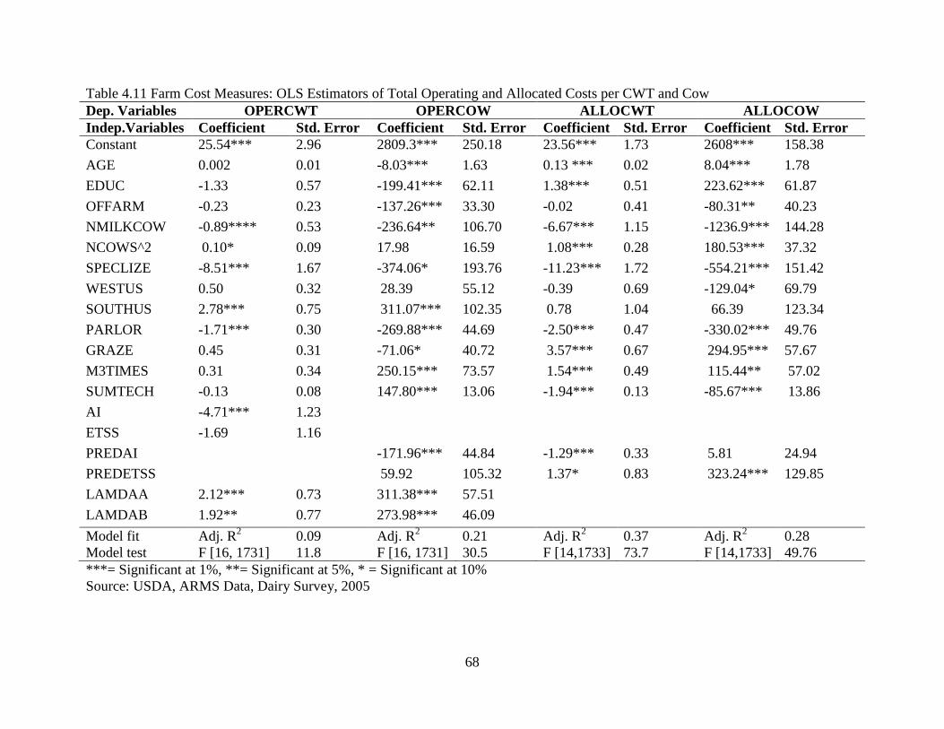
68
Table 4.11 Farm Cost Measures: OLS Estimators of Total Operating and Allocated Costs per CWT and Cow
Dep. Variables OPERCWT OPERCOW ALLOCWT ALLOCOW
Indep.Variables Coefficient Std. Error Coefficient Std. Error Coefficient Std. Error Coefficient Std. Error
Constant 25.54*** 2.96 2809.3*** 250.18 23.56*** 1.73 2608*** 158.38
AGE 0.002 0.01 -8.03*** 1.63 0.13 *** 0.02 8.04*** 1.78
EDUC -1.33 0.57 -199.41*** 62.11 1.38*** 0.51 223.62*** 61.87
OFFARM -0.23 0.23 -137.26*** 33.30 -0.02 0.41 -80.31** 40.23
NMILKCOW -0.89**** 0.53 -236.64** 106.70 -6.67*** 1.15 -1236.9*** 144.28
NCOWS^2 0.10* 0.09 17.98 16.59 1.08*** 0.28 180.53*** 37.32
SPECLIZE -8.51*** 1.67 -374.06* 193.76 -11.23*** 1.72 -554.21*** 151.42
WESTUS 0.50 0.32 28.39 55.12 -0.39 0.69 -129.04* 69.79
SOUTHUS 2.78*** 0.75 311.07*** 102.35 0.78 1.04 66.39 123.34
PARLOR -1.71*** 0.30 -269.88*** 44.69 -2.50*** 0.47 -330.02*** 49.76
GRAZE 0.45 0.31 -71.06* 40.72 3.57*** 0.67 294.95*** 57.67
M3TIMES 0.31 0.34 250.15*** 73.57 1.54*** 0.49 115.44** 57.02
SUMTECH -0.13 0.08 147.80*** 13.06 -1.94*** 0.13 -85.67*** 13.86
AI -4.71*** 1.23
ETSS -1.69 1.16
PREDAI -171.96*** 44.84 -1.29*** 0.33 5.81 24.94
PREDETSS 59.92 105.32 1.37* 0.83 323.24*** 129.85
LAMDAA 2.12*** 0.73 311.38*** 57.51
LAMDAB 1.92** 0.77 273.98*** 46.09
Model fit Adj. R2 0.09 Adj. R
2 0.21 Adj. R
2 0.37 Adj. R
2 0.28
Model test F [16, 1731] 11.8 F [16, 1731] 30.5 F [14,1733] 73.7 F [14,1733] 49.76
***= Significant at 1%, **= Significant at 5%, * = Significant at 10%
Source: USDA, ARMS Data, Dairy Survey, 2005
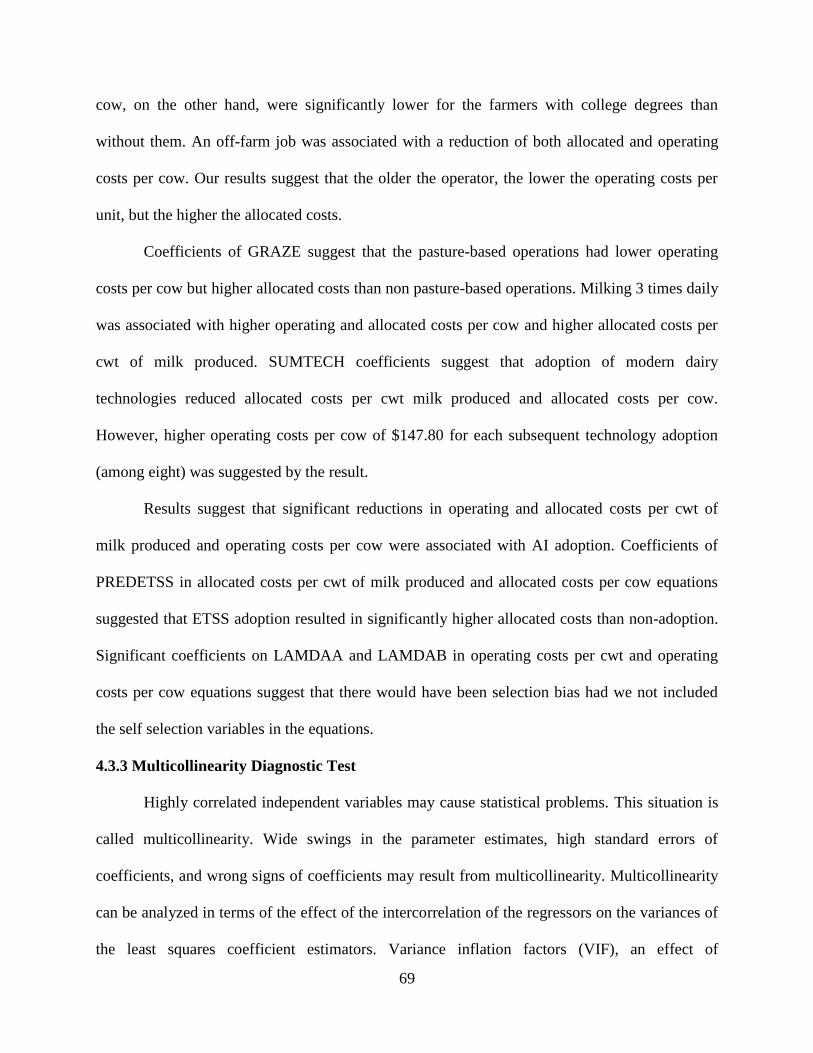
69
cow, on the other hand, were significantly lower for the farmers with college degrees than
without them. An off-farm job was associated with a reduction of both allocated and operating
costs per cow. Our results suggest that the older the operator, the lower the operating costs per
unit, but the higher the allocated costs.
Coefficients of GRAZE suggest that the pasture-based operations had lower operating
costs per cow but higher allocated costs than non pasture-based operations. Milking 3 times daily
was associated with higher operating and allocated costs per cow and higher allocated costs per
cwt of milk produced. SUMTECH coefficients suggest that adoption of modern dairy
technologies reduced allocated costs per cwt milk produced and allocated costs per cow.
However, higher operating costs per cow of $147.80 for each subsequent technology adoption
(among eight) was suggested by the result.
Results suggest that significant reductions in operating and allocated costs per cwt of
milk produced and operating costs per cow were associated with AI adoption. Coefficients of
PREDETSS in allocated costs per cwt of milk produced and allocated costs per cow equations
suggested that ETSS adoption resulted in significantly higher allocated costs than non-adoption.
Significant coefficients on LAMDAA and LAMDAB in operating costs per cwt and operating
costs per cow equations suggest that there would have been selection bias had we not included
the self selection variables in the equations.
4.3.3 Multicollinearity Diagnostic Test
Highly correlated independent variables may cause statistical problems. This situation is
called multicollinearity. Wide swings in the parameter estimates, high standard errors of
coefficients, and wrong signs of coefficients may result from multicollinearity. Multicollinearity
can be analyzed in terms of the effect of the intercorrelation of the regressors on the variances of
the least squares coefficient estimators. Variance inflation factors (VIF), an effect of
70
intercorrelation of the regressors on the variance of least squares coefficient estimates, can be
used to diagnose multicollinearity. Following is the general formula of VIF: ,
where is the obtained when the k
th regressor is regressed on the remaining variables. There
is no consensus on what values of the variance inflation factor suggest multicollinearity. Some
authors suggest values greater than 10 suggest problems (Chatterjee and Price, 1991), while
others suggest 30 or 40 as the benchmark value (Greene, 2009: LIMDEP version 9). Table 4.12
shows the VIF of each variable. Results suggest that none of the variables seems problematic.
Table 4.12: Results of Multicollinearity Diagnostic Test
Variables Variance Inflation Factor
Constant 0
TENYEARS 1.13
AGE 1.08
EDUC 1.08
OFFARM 1.04
NMILKCOW 6.72
NCOWS^2 5.01
SPECLIZE 1.08
WESTUS 1.40
SOUTHUS 1.26
PARLOR 1.43
GRAZE 1.21
M3TIMES 1.48
SUMTECH 2.05
AI 1.23
ETSS 1.12
71
CHAPTER 5
SUMMARY AND CONCLUSIONS
5.1 Summary
Milk production is one of the important components of U.S. agriculture. Milk has a farm
value of production second after beef among livestock industries. The trend in the dairy industry
shows that milk production per cow is significantly increasing while the number of milk cows is
decreasing. Overall milk production per year is increasing despite the declining milk cow
numbers. This increase in productivity is attributed to advancements and adoption of modern
dairy technologies. Breeding technologies are one of the important components of this structural
change in dairy as they directly affect genetics and reproductive performance of the farm. The
adoption decision of modern breeding technologies such as AI, ET, and sexed semen on the
dairy farm is affected by several socioeconomic, demographic, and other factors. Past literature
provides ample technical description of technologies and their methods of operation. However,
the factors associated with the adoption decisions of these breeding technologies and their actual
impacts on farm profitability have not been understood. This study analyzed the factors affecting
the adoption of AI, and ET and/or sexed semen, and their impacts on farm profitability. First, the
characteristics of adopters and non-adopters of these breeding technologies were assessed. Then,
adoption decision models and farm impact models were estimated.
The dairy version of the ARMS, 2005, was used for this study. Altogether, there were
1,814 usable observations in the data. Previous studies have explained AI as a widely adopted,
farmer-friendly technology and ET and sexed semen technologies as relatively newer, still
diffusing technologies. Embryo transplant and sexed semen technologies are suggested to have
potentially wider adoption in the near future. Consistent with previous findings, our results also
72
suggest wider adoption of AI (around 79% of farms). Embryo transplant and/or sexed semen
technologies were adopted by around 11% of dairy farms in 2005. We attempted to account for
the probable correlation of the adoption decisions of these breeding technologies, different from
most of the adoption studies where separate probit equations were generally used. Results from
two separate probits for these two adoption equations are also shown. The assumption of
potential correlation between adoption decisions was confirmed by a formal statistical test. A
correlation coefficient term (correlation between the error terms of two individual probit
equations) significantly different from zero suggested the use of a bivariate probit model rather
than individual probits.
This study also explored some technical and practical patterns of how these breeding
technologies are operated on the farm. There is the involvement of semen that has been collected
by artificial means in the use of both ET and sexed semen. The use of ETSS requires that sperm
will have been collected, artificially, whether or not both or all three technologies are adopted on
the same farm. Since there would be very few cases where ETSS were used by farmers without
AI, adopters of the former could actually be considered as a subset of the latter, implying
selection. This suggested the selection based on AI (i.e., AI adopters select either to use or not
use ETSS). Thus, a bivariate probit with selection model was used to study the adoption.
Relatively younger and more educated farmers had higher probabilities of adoption of
both breeding technologies. The significant negative total marginal effect of age suggested that
younger farmers are the more likely adopters of breeding technologies. Embryo transplant and
sexed semen technologies being relatively newer, a stronger marginal effect of age in the ETSS
equation than that in AI further supports that younger people are more receptive to new ideas
regarding the adoption of technology. The result also supports previous findings about education
and the information-demanding nature of breeding technologies, as breeding technologies were
73
considered “knowledge and information intensive” (Johnson and Ruttan, 1997). Our results
suggested that as farms become more specialized in dairy, the probability of breeding technology
adoption increases. More specialized farms are more focused on higher milk production and may
be interested in adopting the technologies that have short-term as well as long-term effects on
milk production. Furthermore, farms with longer planning horizons of continuing operation for
10 years or more had higher probabilities of breeding technology adoption. The longer planning
horizon was also significant in the separate probit equation of ETSS, but not that of AI. This
further provides insight about the adoption decision in relation to the nature of the technologies.
The ET involves increased reproductive performance of the female and sexed semen
allows the farmer to increase the supply of replacement heifers. Thus, these technologies are not
adopted simply to increase the current season‟s milk yield, but for long-term economic benefits.
As ETSS involves more technical expertise and demands more specialized equipment, farmers
planning to be in the business over an extended period may be more interested in purchasing the
necessary equipment and developing the human resources needed for successful adoption. The
finding of a negative effect of an off-farm job on probability of adoption is as expected, as
breeding technologies are management-intensive. Our results support that the hypothesis that
probability of adoption increases with an increase in the number of milk cows. This suggests that
larger farms are the more likely adopters of breeding technologies.
Farm productivity and profitability were analyzed by estimating the impacts of
demographics and socio-economic factors, adoption of other technologies, and regional
differences on net returns, milk yield per cow, farm revenues, and farm costs equations using
least squares regressions. The actual assessment of the farm impact due to technology adoption is
always an issue in impact studies. To assess the impact of a particular technology, we need to
74
isolate the effects through appropriate correction procedures. In this study, endogeneity and self-
selection bias issues were tested in each equation and corrected when necessary.
Principal operator‟s age negatively affected most of the profitability measures and annual
milk yield per cow. Farmers having a college degree or beyond received higher net returns over
total and operating costs on both per cwt and cow bases. This suggests that younger and more
educated operators can better manage the farm for higher net returns. Principal operator and/or
spouse‟s work off the farm negatively affected net returns over operating costs per cow, around
$73 less than those not working off-farm. Off-farm work also affected milk yield per cow.
Having an off-farm job results in less time available for on-farm work, and thus might have
resulted in lower efficiency of the farm.
Profitability and productivity also depended on the number of milk cows in the operation.
Our results suggest that, with an increase in farm size, net returns over costs per cwt of milk
produced and per cow increase. These results suggest the dairy industry has significant
associated economies of size. Our results also clearly show that an increase in farm size is
significantly associated with decreases in both operating and allocated costs, and thus an increase
in net returns. As farms became more specialized in dairy, they were able to reduce both
operating and allocated costs on both per cow and per cwt of milk produced bases. This less
proportional increase in costs associated with size and specialization results in significant
positive net returns over costs and higher milk yield per cow.
Results suggest that the adoption of modern dairy technologies is associated with higher
net returns over total and operating costs, in general. Though profit depends on the nature of a
specific technology, adoption of modern dairy technologies is associated with higher net returns
over costs in general. A higher return over total costs per cow of $139.26 was associated with
each subsequent adoption of modern technology (among eight considered in this study). On the
75
bases of both per cow and per cwt of milk produced, the farmer having a parlor incurred lower
operating and allocated costs, resulting in higher net returns over both total and operating costs.
Some previous studies also suggested lower costs per unit with parlor adoption for larger farms,
though a parlor is considered as capital intensive (Tauer, 1998; Katsumata and Tauer, 2008).
Results suggested that milking 3 times per day involved both higher allocated and operating
costs. Our result showed slightly higher total costs than revenues per cwt of milk produced,
though this was not significant on a per cow basis. Farms milking 3 times daily had higher milk
yields, a higher yield of 20.88 cwt of milk per cow annually than those milking 2 times or less.
Grazers (pasture based operations) had higher allocated costs and lower operating costs
than non-pasture based operations. Milk yield per cow was lower for pasture-based operations.
Total costs were higher than total revenues for grazers, resulting in negative net returns over total
costs on both per cow and per cwt milk bases. Pasture-based operations require larger land area
for grazing than non-pasture based operations. So, the higher allocated cost results from the cost
of land. Our findings regarding costs and net returns are as expected and consistent with previous
findings regarding pasture-based operations.
We accounted for endogeneity and self-selection issues that might have incurred in the
impact study of breeding technologies. Thus, the coefficients about breeding technologies in this
study are expected to be closer approximations than those not accounting for the issue. Results
suggested AI to be a significantly profitable breeding technology on both per cwt milk produced
and per cow bases. Higher milk yield per cow was associated with AI adoption. AI adopters were
more efficient in reducing total costs than non-adopters. Results also showed the major portion
of the total costs involved in AI come from operating costs rather than allocated costs. Embryo
transplant and/or sexed semen adoption was also suggested to result in higher milk yield and
positive net returns over total and operating costs per cwt milk produced. The impacts on net
76
returns over total and operating costs per cow were non-significant. Results of cost equations
suggested that a higher allocated cost per cow is involved in ETSS adoption. Total costs involved
on a per cow basis were also suggested to be higher with ETSS adoption than non-adoption.
Despite the significantly higher costs, a positive net return over total and operating costs per cwt
milk produced was experienced by ETSS adopters since it was associated with higher milk yield
per cow.
Our results suggest positive, significant, and higher net returns over total and operating
costs associated with both AI and ETSS adoption, at least on a per cwt milk produced basis.
Higher allocated costs were suggested to be involved in ETSS adoption while the major portion
of total costs in AI comes from operating expenses. The coefficient of ETSS should be
interpreted accordingly because we have assumed ETSS adoption as a subset of AI adoption
based on the observations and practicality. This suggests that the ETSS adopters are also the AI
adopters and AI adopters select for ETSS adoption. So, the impact we see on ETSS in our study
also encompasses AI. In the rare cases where ETSS is adopted without AI, the impact of ETSS
on farm profitability and productivity may be different from our result.
5.2 Conclusions and Recommendations
This study showed that adoption of breeding technologies in the U.S. was influenced by
farm characteristics, operator characteristics, adoption of other technologies, and regional
differences. The study also showed the impact of demographics and socio-economic factors,
adoption of other technologies, and regional differences on net returns, milk yield per cow, farm
revenues, and farm costs. The following conclusions and recommendations can be drawn from
our results:
Breeding technologies, affecting reproductive performance of the herd and productivity
and profitability, play an important role in the profitability of dairy farms.
77
Artificial insemination and ET and/or sexed semen adopters, in general, have more milk
cows, are relatively younger and more educated, and produce higher milk yield per cow
than non-adopters. The farms having longer planning horizons are the more likely
adopters of ETSS.
More accurate impact assessment of a particular technology on profitability requires
isolation of that from others. Depending upon the case, accounting for endogeneity and
self-selection issues in impact studies can correct bias and provide more approximate
estimates.
Our results suggest positive, significant, and higher net returns over total and operating
costs associated with both AI and ETSS adoption, at least on a per cwt milk produced
basis. Higher allocated costs were found to be involved in ETSS adoption while the
major portion of total costs in AI comes from operating expenses.
Our findings regarding size and specialization suggest that the larger and more
specialized farms are the recipients of higher net returns. Based on our results, dairy
farms can increase size to capture the higher net returns. The adoption of ETSS may help
increase the number of milk cows by increasing the supply of replacement heifers, but
significant allocated cost involved in the adoption should also be considered.
Since some part of the costs involved in ETSS may be for conducting artificial
insemination, larger farms that had already adopted AI may consider ETSS adoption.
Adoption decisions on a farm, however, would be based on the added advantages of
ETSS adoption versus the additional costs of adopting these.
In addition to costs, technical knowledge and information requirements for breeding
technologies could be a hindrance in the diffusion of breeding technologies, particularly
ETSS. Extension agents and/or specialists are suggested to consider more educated,
78
younger farmers with larger farms as quick adopters of breeding technologies. Further,
farms that plan to continue operation for a number of years are suggested to be potential
ETSS adopters.
5.3 Limitations
Based on the literature, we said that ETSS allows for an increased supply of replacement
heifers and improved reproductive performance in the herd. We also suggested that farmers
judge the advantages accordingly. One of the limitations and beyond the scope of this study is
determining the actual number of replacement heifers produced or how much reproductive
performance is improved annually on a particular farm due to the adoption of ETSS. Another
limitation we faced using ARMS data was the inseparability between ET and sexed semen
adopters. Since the ARMS question was designed such that they were not separated, we have
treated ET and/or sexed semen as one technology, “ETSS.” Though the adopters of these
technologies may have similar traits, the results and implications when they are treated
separately may be different.
Sexed semen technology is expanding and is expected to have wider adoption in the near
future. The actual impact of the sexed semen technology, once when it becomes more diffused
would be a further interest of study. Since farmer‟s perceptions about the profitability of the
technology may also affect the adoption decision, inclusion of perception questions in the ARMS
dairy survey could lead to more insights.
79
REFERENCES
Abdulai, A and W. E. Huffman. "The Diffusion of New Agricultural Technologies: The Case of
Crossbred-Cow Technology in Tanzania." American Journal of Agricultural Economics
87, 3 (2005): 645-659
Abdulai, A., P. Monnin and J. Gerber. “Joint Estimation of Information Acquisition and
Adoption of New Technologies under Uncertainty” Journal of International
Development 20 (2008): 437-451
Amos, H.E., T. Kiser, and M. Lowenstein. “Influence of Milking Frequency on Productive and
Reproductive Efficiencies of Dairy Cows.” Journal of Dairy Science 68 (1985): 732.
Arendonk, J., Van, M., and Bijma, P. “Factors Affecting Commercial Application of Embryo
Technologies in Dairy Cattle in Europe-A Modeling Approach.” Theriogenology 59
(2003): 635-649.
Bandiara O. and I. Rasul. “Social Networks and Technology Adoption in Northern
Mozambique.” Economic Journal 116 (October 2006): 869-902.
Barber, K.A. “Maximizing the Impact of Dairy and Beef Bulls through Breeding Technology.”
Journal of Dairy Science 66 (1983): 2661-2671.
Besley, T. and A. Case. “Modeling Technology Adoption in Developing Countries.” The
American Economic Review 83, 2. Papers and Proceedings of the Hundred and Fifth
Annual Meeting of the American Economic Association (May, 1993): 396-402.
Boyes W. J., D. L. Hoffman, and S. A. Low. “An Econometric Analysis of the Bank Credit
Scoring Problem.” Journal of Econometrics 40 (1989): 3-14.
Britt, J. H. “Enhanced Reproduction and Its Economic Implication.” Journal of Dairy Science
68 (1985): 1585-1592.
Burton, M., D. Rigby, and T. Young. “Analysis of the Determinants of Adoption of Organic
Horticultural Techniques in the U.K.” Journal of Agricultural Economics 50, 1 (1999):
47-63.
Busem, R.C., and Bromley, D.W. Applied Economics. Iowa State Univ. Press, Ames. 1975.
Caswell, M. and D.Zilberman. “The Choices of Irrigation Technologies in California.” American
Journal of Agricultural Economics (May 1985).
Chatterjee, S. and B. Price. Regression Analysis by Example, Second Edition. John Wiley and
Sons (1991).
80
Cooper, J. C. and R. W. Keim. "Incentive Payments to Encourage Farmer Adoption of Water
Quality Protection Practices." American Journal of Agricultural Economics 78, 1 (1996):
54-64.
Dartt, B. A., J. W. Lloyd, B. R. Radke, J. R. Black, and J. B. Kaneene. “A Comparision of
Profitability and Economics between Management-intensive Grazing and
Conventionality Managed Dairies in Michigan.” Journal of Dairy Science 82 (1999):
2412-2420.
DePeters, E.J., N.E. Smith, and J. Acedo-Rico.“Three or Two Times Daily Milking of Older
Cows and First Lactation Cows for the Entire Lactation.” Journal of Dairy Science
68(1985):123.
DeVries, A., M. Overton, J. Fetrow, K. Leslie, S. Eicker, and G. Rogers. “Exploring the Impact
of Sexed Semen on the Structure of the Dairy Industry.” Journal of Dairy Science 91, 2
(2008): 847-856.
Dorfman, J. H. "Modeling Multiple Adoption Decisions in a Joint Framework." American
Journal of Agricultural Economics 78, 3 (1996): 547-557.
Dubman, R.W. Variance Estimation with USDA‟s Farm Costs and Returns Surveys and
Agricultural Resource Management Study Surveys. Staff Paper AGES 00-01, USDA-
ERS, April 2000.
Eli-Lilly website accessed July 13, 2009: http://www.elancodairy.com/about/benefits/index.html.
El-Osta, H.S, and J. D. Johnson. “Determinants of Financial Performance of Commercial Dairy
Farms.” Technical Bulletin no. 1859, USDA-ERS, (July 1998).
El-Osta, H.S. and M. J. Morehart. “Technology Adoption and Its Impact on Production
Performance of Dairy Operations. Review of Agricultural Economics 22, 2 (2000):477-
498.
El-Osta, H.S., A. K. Mishra, and M. J. Morehart. “Determinants of Economic Well-Being
Among U.S. Farm Operator Households.” Agricultural Economics 36 (2007): 291-30.
Erdman, R. A. and M. Varner. “Fixed Yield Response to Increased Frequency.” Journal of Dairy
Science 78 (1995): 1199-1203.
Feder, G., Just, R.E., and Zilberman,D. “Adoption of Agricultural Innovations in Developing
Countries.” Economic Development and Cultural Change 33 (1985): 255-29.
Fernedez-Cornejo J. and W. D. McBride. “Adoption of Bioengineered Crops.” Agricultural
Economic Report No. 810. Economic Research Service, United States Department of
Agriculture, Washington, DC (2002).
81
Fernendez-Cornejo J. “Off-farm Income, Technology Adoption, and Farm Economic
Performance.” Economic Research Report No. 36. USDA, ERS, (January 2007).
Fernendez-Coenejo J., C. Hendrix, and A. Mishra. “Technology Adoption and Off-Farm
Household Income: The Case of Herbicide-Tolerant Soybeans.” Journal of Agricultural
and Applied Economics 37, 3 (December 2005): 549-563.
Fernendez –Cornejo J., C. Klotz-Ingram, and S. Jans. “Farm Level Effects of Adopting
Herbicide-Tolerant Soybeans in the U.S.A.” Journal of Agricultural and Applied
Economics 34, 1 (April 2002): 149-163.
Foltz, J. and Chang, H.H. “The Adoption and Profitability of rbST on Connecticut Dairy Farms.”
American Journal of Agricultural Economics 84 (2002):1021-1032.
Foltz, J. and G. Lang. “The Adoption and Impact of Management Intensive Rotational Grazing
on Connecticut Dairy Farms.” Renewable Agriculture and Food Systems 20, 4 (2005):
261-266.
Foote, R.H. “Review: Dairy Cattle Reproductive Physiology Research and Management - Past
Progress and Future Prospects.” Journal of Dairy Science 79 (1996): 980-990.
Freedman, D. A. and J. S. Sekhon. “Endogeneity in Probit Response Models (May 29 2008).
Available at: http://ssrn.com/abstract=1138489.
Funk, D. A. "Major Advances in Globalization and Consolidation of the Artificial Insemination
Industry." Journal of Dairy Science 89, 4(2006): 1362-1368.
Ghosh, S., J.T. McGuckin and S. C. Kumbhakar “Technical Efficiency, Risk Attitude,
and Adoption of New Technology: The Case of the US Dairy Industry” Technological
Forecasting and Social Change. 46 (1994): 269-278.
Gillespie J., R. Nehring, C. Hallahan, and C. Sandretto. “Pasture-Based Dairy Systems: Who Are
the Producers and Are their Operations More Profitable than Conventional Dairies?”
Journal of Agricultural and Resource Economics, 34, 3 (2009): 412-427.
Gillespie, J., T. Mark, C. Sandretto, and R. Nehring. “Computerized Technology Adoption
Among Farms in the U.S. Dairy Industry.” Journal of American Society of Farm
Management and Rural Appraisers (2009): 216-224.
Gillespie, J.M., C.G. Davis, and N.C. Rehelizatovo. "Factors Influencing the Adoption of
Breeding Technologies in U.S. Hog Production." Journal of Agricultural and Applied
Economics 36 (2004): 35-47.
Gisi, D.D., E.J. DePeters and C. L. Pelissier. “Three Times Daily Milking of Cows in California
Dairy Herds.” Journal of Dairy Science 69 (1986): 863.
82
Goff, K.R. “Three x Daily Milking: A Study of Production and Economic Gain in Six 3x Herds.”
Mimeo University of Connecticut 1977.
Greene, W. H. “A Statistical Model for Credit Scoring.” Working Paper No. EC-92-29,
Department of Economics, Stern School of Business, New York University (1992).
Greene, W. H. "Marginal Effects in the Bivariate Probit Model." EC-96-11 SSRN eLibrary (June
1996).
Greene, W. H., Econometric Analysis, 6th
Edition. New York University. Upper Saddle River,
NJ: Prentice-Hall, 2008.
Greene, W. H., LIMDEP, Version 9, Econometric Modeling Guide. New York: Econometric
Software, Inc., 2009.
Greene, W.H. Econometric Analysis. 4th
Edition. Printice-Hall, Upper saddle River, NJ 2000.
Griliches, Z. “Hybrid Corn: An Exploration in Economics of Technological Change.”
Econometrica 25 (October 1957): 501-522.
Grisham E. “Record Keeping Systems Adoption by Louisiana Dairy Farmers.” MS Thesis,
Louisiana State University, 2007.
Hammond, J. W. “Trends in the Size Distribution of Dairy Farms in Minnesota and Wisconsin.”
Staff Paper P94-27. University of Minnesota, (December 1994).
Hanson G.D., L. C. Cunningham, S. A. Ford, L.D. Muller, and R.L. Parsons. “Increasing
Intensity of Pasture Use with Dairy Cattle: An Economic Analysis.” Journal of
Production Agriculture 11, 2 (1998): 175-179.
Hasler, J.F. “Current Status and Potential of Embryo Transfer and Reproductive Technology in
Dairy Cattle.” Journal of Dairy Science 75, 10 (1992): 2857-2879.
Heckman J. “Sample Selection Bias as a Specification Error.” Econometrica, 47 (1979): 153-
161.
Herbst, B. K., D. P. Anderson, J. L. Outlaw, J.W. Richardson, and T. Bilby. “The Effects of
Sexed-Sorted Semen on Southern Dairy Farms.” Selected paper for presentation at the
Southern Agricultural Economics Association Annual Meeting. Atlanta, Georgia, Jan.31-
Feb 3, 2009.
Hill R. C., W. E. Griffiths, and G. C. Lim. Principles of Econometrics, Third Edition. John
Wiley and Sons, Inc., Hoboken NJ (2008).
Hillers, J.K., S.C. Thonney, and C. T. Gaskins. “Economic Comparison of Breeding Dairy Cows
Artificially Versus Naturally.” Journal of Dairy Science 65, 5 (1982).

83
Johnson, N.L., and V. W. Ruttan. “The Diffusion of Livestock Breeding Technology in the US:
Observations on the Relationship between Technical Change and Industry Structure.”
Journal of Agribusiness 15, 1(1997): 19-35.
Kaplan D. and R. L. Venezky. “Literacy and Voting Behaviour: A Bivariate probit Model with
Sample Selection.” Social Science Research 23 (1994): 350-367.
Katsumata, K., and L. Tauer. “Empirical Analysis of Stanchion and Parlor Milking Cost on New
York Dairy Farms.” Selected paper for Annual Meetings of the Southern Agricultural
Economic Association, Dallas (2008).
Kelly, A.L. Primary Milk Production. In: Mechanization and Automation in Dairy Technology.
T.Y. Adnam and B.A. Law, ed. Sheffield Acad. Press, UK (2001): 40-47.
Khanal, A. R., J. Gillespie and J. MacDonald. “Adoption of Technology, Management Practices,
and Production Systems in U.S. Milk Production.” Selected paper for Annual Meeting of
Southern Agricultural Economics Association (SAEA), Orlando, Florida (2010).
Kruip, T.A.M., J. Stefanowska, and W. Ouweltjes. “Robot Milking and Effect on Reproduction
in Dairy Cows: A Preliminary Study.” Animal Reproduction Science 2016. (2000): 1-5.
LIMDEP, Version 8 and 9, Econometric Modeling Guide. Econometric Software Inc. Plainview,
NY 11803, USA.
Long J. S. and L. H. Ervin. “Using Heteroskedasticity Consistent Standard Errors in the Linear
Regression Model.” The American Statistician 54, 3 (2000): 217-224.
Lush, J.L. and R.R. Shrode, “Changes in Milk Production with Age and Milking Frequency.”
Journal of Dairy Science 33 (1950): 338.
MacDonald, J.M., E. J. O‟Donoghue, W. McBride, R. Nehring, C. L. Sandretto, and R.
Mosheim. Profits, Costs and the Changing Structure of Dairy Farming. ERR-47, USDA-
ERS 2007.
Manchester, A.C. and D. P. Blayney. The Structure of Dairy Markets: Past, Present, Future.
Agricultural Economic Report 757, USDA-ERS 1997.
Massey C., S. Morris, F. Alpass and R. Flett. “A Framework for Building Technological
Learning: Evidence from the New Zealand Dairy industry.” Journal of Extension 42, 3
(January 2004).
McBride, W.D., S. Short, and H. El-Osta. “The Adoption and Impact of Bovine Somatotropin on
U.S. Dairy Farms.” Review of Agricultural Economics 26, 4 (2004): 472-488.
Medical News Today. Microbix Establishes Key Global Distribution Agreements For Its
SST(TM) Sperm Sexing Technology For The Dairy, Beef And Swine Industries. Article
84
date: 14 July, 2006. Internet site: http://www.medicalnewstoday.com/articles/47043.php
(Accessed July 9, 2009).
Meng, C. and Schmidt, P. “On the Cost of Partial Observability in the Bivariate Probit Model.”
International Economic Review 26, 1 (1985): 71-86.
Microbix Biosystems Inc. Sperm Sexing Technology. Internet site:
http://www.microbix.com/Public/Default.aspx?I=75 (Accessed July 9, 2009).
Mishra A.K. and H. S. El-Osta. “Effect of Agricultural Policy on Succession Decisions of Farm
Households.” Review of Econ Household, 6 (2008): 285-307.
Mohanty M. S. “A Bivariate Probit Approach to the Determination of Employment: A Study of
Teen Employment Differentials in Los Angeles County.” Applied Economics 34 (2002):
143-156.
Moreno, G. and D. L. Sunding “Simultaneous Estimation of Technology Adoption and Land
Allocation.” Paper prepared for presentation at the American Agricultural Economics
Association Annual Meeting, Montreal, Canada, July 27-30, 2003.
Moreno, G. and D. L. Sunding. “Joint Estimation of Technology Adoption and Land Allocation
with Implications for the Design of Conservation Policy.” American Journal of
Agricultural Economics 87(2005): 1009-1019.
National Agricultural Statistics Service (USDA/ NASS). Quick Stats. USDA, October 2009.
Nicholson, C.F, P.K. Thronton, L. Mohammed, R.W. Muinga, D.M. Mwamachi, E.H. Elbasha,
S.J. Staal and W. Thorpe. Smallholder Dairy Technology in Costal Kenya, An Adoption
and Impact Study. ILRI Impact Assessment Series 5. International Livestock Research
Institute, Nairobi, Kenya 1999.
Obubuofo J., J. Gillespie, K. Paudel, and S. Kim. “Awareness of and Application to
Environmental Quality Incentive Programs by Cow-Calf Producers.” Journal and
Agricultural and Applied Economics 40, 1 (2008): 357-368.
Olynk, N.J and C. A. Wolf. “A Survey of Reproductive Management Strategies on US
Commercial Dairy Farms.” Staff paper 2008-02, Department of Agricultural, Food and
resource Economics, Michigan State University. (2008 May).
Pearson, R.E., L.A. Fulton, P.D. Thompson, and J.W. Smith. “Three Times a Day Milking
During the First Half of Lactation.” Journal of Dairy Science 62 (1979): 1941.
Pelissier, C.L., L.J. Koong, and L.F. Bennett. “Influence of Milking 3 Times Daily on Milk and
Fat Production.” Journal of Dairy Science 61, 1 (1978): 132.
Poole, D.A.. “The Effects of Milking Cows Three Times Daily.” Animal Production 34. p. 187.

85
Purdy B. M., M. R. Langemeier, and A. M. Featherstone. “ Financial Performance, Risk, and
Specialization.” Journal of Agricultural and Applied Economics, 29, 1 (1997): 149-161.
Rogers, E. M. Diffusion of Innovations (Rev. ed.). New York, NY: Free Press.1999.
Rogers, E. M. Diffusion of Innovations (5th ed.). New York, NY: Free Press. 2003.
Seidel, G. E., Jr. "Applications of Embryo Transfer and Related Technologies to Cattle." Journal
of Dairy Science 67, 11(1984): 2786-2796.
Shook, G.E. “Major Advances in Determining Appropriate Selection Goals.” Journal of Dairy
Science 89. (2006): 1349-1361.
Short, S.D. “Characteristics and Production Costs of US Dairy Operations.” Statistical Bulletin
no. 974-6, USDA-ERS, 2004.
Short, S.D. “Structure, Management, and Performance Characteristics of Specialized Dairy Farm
Businesses in the United States.” Agriculture Handbook no. 720, USDA-ERS, September
2000.
Shumway, C. R., R.W. Brake, D. J. Leatham and M. A. Tomaszewesky. “Economics of a
Biotechnology: Artificial Insemination Dairy Sires.” Agribusiness 3, 2 (1987): 207-220.
Smeaton, D. C., B. L. Harris, Z. Z. Xu and W. H. Vivanco. "Factors Affecting Commercial
Application of Embryo Technologies in New Zealand: A Modelling Approach."
Theriogenology 59, 2 (2003): 617-634.
Sorensen, A., D.D. Muir, and C. H. Knight. “Thrice-daily Milking throughout Lactation
Maintains Epithelial Integrity and Thereby Improves Milk Protein Quality.” Journal of
Dairy Research 68 (2001): 15-25.
Spain, J.N, and M. Witherspoon. “Why Missouri Dairy Farms Discontinue Dairy Herd
Improvement Association Testing Programs.” Journal of Dairy Science 77, 4 (1994):
1141-1145.
Tauer, L. W. “The Estimated Profit Impact of Recombinant Bovine Somatotropin on New York
Dairy Farms for The Years 1994 Through 1997” AgBioForum 4, 2 (2001).
Tauer, L.W. “Cost of Production for Stanchion Versus Parlor Milking in New York.” Journal of
Dairy Science 81(1998): 567-569.
Tauer, L.W. “The Impact of Recombinant Bovine Somatotropin on Dairy Farm Profits: A
Switching Regression Analysis.” AgBioForum 81 (2005): 33-39.
Tauer, L.W., and A. K. Mishra. “Dairy Farm Cost Efficiency.” Journal of Dairy Science 89,12
(2006): 4937-4943.
86
Taylor, J., and J. Foltz. “Grazing in the Dairy State: Pasture Use in the Wisconsin Dairy Industry,
1993-2003.” Report provided by Department of Agricultural and Applied Economics,
University of Wisconsin, Medison, January 2006.
Tyler, H., and M. Ensminger, M. Dairy Cattle Science. Prentice-Hall, Upper Saddle River, NJ
(2005).
U.S. Department of Agriculture, National Agricultural Statistics Service. Land, Land in Farms,
and Livestock Operations: 2008 Summary. (February 2009).
United States Department of Agriculture (USDA) Report to Congress. Economic Effects of US
Dairy Policy and Alternative Approaches to Milk Pricing. (July 2004).
United States Department of Agriculture (USDA), National Agriculture Statistics Services
(NASS). “Milk Production, Disposition and Income 2008 Summary” Da 1-2 (09) (May
2009).
United States Department of Agriculture, National Agricultural Statistics Service. “Milk
Disposition and Income Final Estimates 2003-2007.” Statistical Bulletin Number 1027.
(May 2009).
United States Department of Agriculture, National Agricultural Statistics Service. “Milk Cows
and Production Final Estimates 2003-2007.” Statistical Bulletin Number 1022. (March
2009).
Van De Ven, W. P. M. M. and B. M. S. Van Praag. “The Demand for Deductibles in Private
Health Insurance.” Journal of Econometrics 17 (1981): 292-252
Vella F. and M. Verbeek. “Estimating and Interpreting Models with Endogenous Treatment
Effects.” Journal of Business and Economic Statistics 17, 4 (Oct. 1999): 473-478.
Wahba, J. “Returns to Overseas Work Experience: The Case of Egypt.” In: Ozdon C. and Schiff,
M. (eds.) Internation Migration, Economic development and Policy. Washington DC:
The World Bank (2007).
Weersink, A. and L. W. Tauer. “Causality between Dairy Farm Size and Productivity.”
American Journal of Agricultural Economics 73, 4 (1991): 1138-1145.
Weigel, K.A. “Exploring the Role of Sexed Semen in Dairy Production Systems.” Journal of
Dairy Science 87(2004): E120-E130.
Wooldridge, J. M. Introductory Econometrics: A Modern Approach, Third Edition. Thomson
South-Western, Thomson Learning Inc. (2006).
Zepeda, L. “Simultaneity of Technology Adoption and Productivity.” Journal of Agricultural
and Resource Economics 19, 1 (1994): 46-57.
87
VITA
Aditya was born in a very beautiful Himalayan country, Nepal. After completion of his
higher secondary level education in science from New Horizon Higher Secondary School, he
joined Institute of Agriculture and Animal Sciences, Tribhuvan University, Nepal, in 2002. He
completed his bachelor of sciences in agriculture in 2006. Then, he worked as a project officer in
a non-governmental organization called LI-BIRD, Nepal, for two years.
Aditya started his master‟s program in the Department of Agricultural Economics and
Agribusiness at Louisiana State University in the Fall of 2008. Upon completion of his master‟s
degree, Aditya will pursue a doctorate.