adrian costea, phd department of statistics and econometrics vasile … costea (t).pdf ·...

Adrian COSTEA, PhD

Department of Statistics and Econometrics

The Bucharest Academy of Economic Studies

E-mail: [email protected]

Vasile BLEOTU, PhD

Faculty of Finance, Banks and Accounting

“Dimitrie Cantemir” Christian University

A NEW FUZZY CLUSTERING ALGORITHM FOR EVALUATING

THE PERFORMANCE OF NON-BANKING FINANCIAL

INSTITUTIONS IN ROMANIA

Abstract. In this article we propose a modified version of Fuzzy C-

Means (FCM) clustering algorithm in order to better allocate the

uncertain observations in the clusters. We change the objective function of

the classic FCM by attaching different weights to the distances between

observations and the clusters’ centers. We apply the modified FCM

(Weighting FCM) to model the performance of non-banking financial

institutions (NFIs) in Romania. We extend the experiment from our

previous work by improving NFIs’ performance dataset from 3 to 8

performance ratios and from 44 to 769 observations. The results show a

significant improvement in pattern allocation with the new proposed

algorithm.

Key words: fuzzy logic, clustering, Fuzzy C-Means algorithm,

linguistic variables, weights, non-banking financial institutions,

performance evaluation models

JEL classifications: C38, C81, G23

I. Introduction

The evaluation of non-banking financial institutions (NFIs) as to their financial

performance is a research problem that has been recently put on the table by the

practitioners. In Romania, the Supervision Department at National Bank of

Romania developed the Uniform Assessment System or CAAMPL (Cerna et al.,

2008), which constitutes an effective tool for evaluating the performance of credit

institutions. However, this system as such, is not applicable to evaluating the

performance of NFIs because it uses rather simpler one-ratio-at-a-time

discriminating techniques. In our previous work (Costea, 2011a) we formalized the

process of evaluating the performance of NFIs by considering it as a knowledge

discovery process. In this respect, we propose Data Mining techniques to be

mailto:[email protected]

Adrian Costea, Vasile Bleotu

____________________________________________________________ applied for transforming the available data into information and knowledge. We

can formalize the problem of evaluating the performance of NFIs in two ways: as a

description problem or as a prediction problem. In general, clustering techniques

have descriptive properties and classification techniques have predictive ones. In

our previous work (Costea, 2011b), we have applied a neural-network-based

clustering technique, called SOM (Self-Organising Map) algorithm, in order to

analyze comparatively the NFIs in Romania. We have benefited from the algorithm

scalability and visualization capability when we analyzed the results obtained after

running sessions with different choices for the algorithm’s parameters.

In this paper we introduce a descriptive clustering method that is based on the

theory of fuzzy logic for analyzing the NFIs’ sector.

Traditional clustering methods intend to identify patterns in data and create

partitions with different structures (Jain et al., 1999). These partitions are called

clusters and elements within each cluster should share similar characteristics. In

principle, every element belongs to only one partition, but there are observations in

the data set that are difficult to position. In many cases subjective decisions have to

be made in order to allocate these uncertain observations.

In contrast to these methods, fuzzy clustering methods assign different membership

degrees to the elements in the data set indicating in which degree the observation

belongs to every cluster. One traditional method in fuzzy clustering is the Fuzzy C-

Means (FCM) clustering method (Bezdek, 1981). Every observation gets a vector

representing its membership degree in every cluster, which indicates that

observations may contain, with different strengths, characteristics of more than one

cluster. In this situation we usually assign the elements of the data set to the cluster

that has the highest membership degree. In spite of the additional information

provided by the methodology, there is a problem with the observations that are

difficult to position (uncertain observations) when they obtain similar highest

membership values for two or more clusters.

This paper proposes a method to allocate the uncertain observations by introducing

weights to the FCM algorithm. The weights indicate the level of importance of

each attribute in every cluster so that allocation is done depending on the linguistic

classification of the partitions. The data set used corresponds to 8 financial ratios

and 65 NFIs collected quarterly from 2007 to 2010. The results show that the

characterization of the clusters by means of linguistic variables gives an easy to

understand, jet formal, classification of the partitions. Also, when weights are

extracted from these characteristics, the uncertain observations are better allocated.

We discuss the comparison of the results with the classic FCM method.

The paper is organized as follows: in the next section we engage in a thorough

literature review regarding the application of Data Mining methods in assessing

comparatively companies’ financial performance. Then, we present the modified

version of FCM clustering algorithm by introducing some weights to the objective

A new fuzzy clustering algorithm for evaluating the performance of non-banking

financial institutions in Romania

__________________________________________________________________

function of the classic FCM algorithm. Finally, we apply FCM clustering, both the

classic and the modified versions, to assess comparatively the performance of NFIs

in Romania and draw our conclusions.

II. Literature review

The research literature in applying the Data Mining techniques to comparing

different entities consist of: companies’ financial benchmarking, companies’

failure prediction, companies’ credit/bond rating, analysis of companies’ financial

statement, and analysis of companies’ financial text data.

The SOM (Self-organising Map) algorithm was used extensively in assessing

comparatively companies’ financial performance. There are two pioneer works of

applying the SOM to companies’ financial performance assessment. One is Martín-

del-Brío & Serrano Cinca (1993) followed by Serrano Cinca (1996, 1998a, 1998b).

Martín-del-Brío & Serrano Cinca (1993) proposed SOM as a tool for financial

analysis. The sample dataset contained 66 Spanish banks, of which 29 went

bankrupt. Martín-del-Brío & Serrano Cinca (1993) used nine financial ratios,

among which there were three liquidity ratios: current assets/total assets, (current

assets - cash and banks)/total assets, and current assets/loans; three profitability

ratios: net income/total assets, net income/total equity capital, and net

income/loans; and three other ratios: reserves/loans, cost of sales/sales, and cash

flows/loans. A solvency map was constructed, and different regions of low

liquidity, high liquidity, low profitability, high cost of sales, etc. were highlighted

on the map. Serrano Cinca (1996) extended the applicability of SOM to bankruptcy

prediction. The data contain five financial ratios taken from Moody’s Industrial

Manual from 1975 to 1985 for a total of 129 firms, of which 65 are bankrupt and

the rest are solvent. After a preliminary statistical analysis the last ratio (sales/total

assets) was eliminated because of its poor ability to discriminate between solvent

and bankrupt firms. Again, a solvency map is constructed and, using a procedure to

automatically extract the clusters, different regions of low liquidity, high debt, low

market values, high profitability, etc. are revealed. Serrano Cinca (1998a, 1998b)

extended the scope of the Decision Support System proposed in the earlier studies

by addressing, in addition to corporate failure prediction, problems such as: bond

rating, the strategy followed by the company in relation to the sector in which it

operated based on its published accounting information, and comparison of the

financial and economic indicators of various countries.

The other major SOM financial application is Back et al. (1998), which is an

extended version of Back et al. (1996). Back et al. (1998) analysed and compared

more than 120 pulp-and-paper companies between 1985 and 1989 based on their

annual financial statements. The authors used nine ratios, of which four were

profitability ratios (operating margin, profit after financial items/total sales, return

on total assets, return on equity), one was an indebtedness ratio (total

liabilities/total sales), one denoted the capital structure (solidity), one was a


____________________________________________________________ liquidity ratios (current ratio), and two were cash flow ratios (funds from

operations/total sales, investments/total sales). The maps were constructed

separately for each year and feature planes were used to interpret them. An analysis

over time of the companies was possible by studying the position each company

had in every map. As a result the authors claimed that there were benefits in using

SOM to manage large and complex financial data in terms of identifying and

visualizing the clusters.

Eklund et al. (2003) investigated the suitability of SOM for financial benchmarking

of world-wide pulp-and-paper companies. The dataset consists of seven financial

ratios calculated for 77 companies for six years (1995-2000). Eklund et al. (2003)

constructed a single map for all the years and found clusters of similar financial

performance by studying the feature plane for each ratio. Next, the authors used

SOM visualisation capabilities to show how the countries’ averages, the five

largest companies, the best performers and the poorest performers evolved over

time according to their position in the newly constructed financial performance

clusters. Karlsson et al. (2001) used SOM to analyse and compare companies from

the telecommunication sector. The dataset consists of seven financial ratios

calculated for 88 companies for five years (1995-1999). Karlsson et al. (2001) used

a similar approach to Eklund et al. (2003) and built a single map. The authors

identify six financial performance clusters and show the movements over time of

the largest companies, countries’ averages and Nordic companies. Both Eklund et

al. (2003) and Karlsson et al. (2001) used quantitative financial data from the

companies’ annual financial statements. The ratios were chosen based on

Lehtinen’s (1996) study of the validity and reliability of ratios in an international

comparison. Kloptchenko (2003) used the prototype matching method (Visa et al.,

2002; Toivonen et al., 2001; Back et al., 2001) to analyse qualitative (text) data

from telecom companies’ quarterly reports. Kloptchenko et al. (2004) combined

data and text-mining methods to analyse quantitative and qualitative data from

financial reports, in order to see if the textual part of the reports could offer support

for what the figures indicated and provided possible future hints. The dataset used

was from Karlsson et al. (2001). Voineagu et al. (2011) used technical analysis

to determine the future price of a share based on the influence coming from

behavioral economics.

C-Means algorithm was applied on the problem of financial performance

benchmarking in conjunction with other techniques. For example, Ong & Abidi

(1999) applied SOM to a 1991 World Bank dataset that contained 85 social

indicators in 202 countries finding clusters of similar performance. Here, the

different performance regions were constructed objectively by applying C-Means

on the trained SOM. Vesanto & Alhoniemi (2000) compared basic SOM clustering

with different partitive (C-Means) and agglomerative (single linkage, average

linkage, complete linkage) clustering methods. At the same time, the authors

introduced a two-stage SOM clustering (similar with our SOM clustering

approach) which consisted of, firstly, applying the basic SOM to obtain a large

number of prototypes (“raw” clusters) and, secondly, clustering these prototypes to



__________________________________________________________________

obtain a reduced number of data clusters (“real” clusters). The partitive and

agglomerative clustering methods were used to perform the second phase of the

two-stage clustering. In other words, these methods were used to group the

prototypes obtained by SOM into “real” clusters. The comparisons were made

using two artificial and one real-world datasets. The comparisons between the

basic SOM and other clustering methods were based on the computational cost.

SOM clearly outperformed the agglomerative methods (e.g., average linkage

needed 13 hours to directly cluster the dataset III, whereas SOM needed only 9.5

minutes). The clustering accuracy (in terms of conditional entropies) was used to

compare the direct partitioning of data with the two-stage partitioning. The results

show that partitioning based on the prototypes of the SOM is much more evenly

distributed (approximately an equal number of observations are obtained in each

cluster). At the same time, the two-stage clustering results were comparable with

the results obtained directly from the data.

The use of fuzzy clustering—especially the Fuzzy C-Means (FCM) algorithm—in

assessing comparatively companies’ financial performance is relatively scarce. The

fuzzy logic approach can also deal with multi-dimensional data and model non-

linear relationships among variables. It has been applied to companies’ financial

analysis, for example, to evaluate early warning indicators of financial crises

(Lindholm & Liu, 2003), or to develop fuzzy rules out of a clustering obtained with

self organizing map algorithm (Drobics et al., 2000). Wang et al. (2009) described

a model for selecting the suppliers based on fuzzy method (TOPSIS). Baležentis &

Baležentis (2011) extend the MULTIMOORA–2T (Multi–Objective Optimization

by Ratio Analysis plus the Full Multiplicative Form – Two Tuples) method for

group multi–criteria decision making under linguistic environment. Two–tuples are

used to represent, convert and map into the basic linguistic term set various crisp

and fuzzy numbers.

One of the pioneer works in applying discriminant analysis (DA) to assess

comparatively companies’ financial performance was Altman (1968). Altman

calculated discriminant scores based on financial statement ratios such as working

capital/total assets, retained earnings/total assets, earnings before interest and

taxes/total assets, market capitalisation/total debt, sales/total assets. Ohlson (1980)

was one of the first studies to apply logistic regression (LR) to predict the

likelihood of companies’ bankruptcy. Since it is less restrictive than other

statistical techniques (e.g., DA), LR has been used intensively in financial analysis.

Pele (2011) uses LR to investigate the connection between the complexity of a

capital market and the occurrence of dramatic decreases in transaction prices. The

market complexity is estimated through differential entropy. De Andres (2001, p.

163) provided a comprehensive list of papers that used LR for models of

companies’ financial distress.

Induction techniques such as Quinlan’s C4.5/C5.0 decision-tree algorithm were

also used in assessing companies’ financial performance. Shirata (2001) used a


____________________________________________________________ C4.5 decision-tree algorithm together with other techniques to tackle two problems

concerning Japanese firms: prediction of bankruptcy and prediction of going

concern status. For the first problem, the authors chose 898 firms that went

bankrupt with a total amount of debt more than ¥10 million. For the going concern

problem, 300 companies were selected out of a total of 107,034 that had a stated

capital of more than ¥30 million. The financial ratios used were: retained

earnings/total assets, average interest rate on borrowings, growth rate of total

assets, and turnover period of accounts payable. As a conclusion of the study, the

author underlined that decisions concerning fund raising can create grave hazards

to business and, therefore, in order to be successful, managers had to adapt to the

changing business environments.

Supervised learning artificial neural networks (ANNs) were extensively used in

financial applications, the emphasis being on bankruptcy prediction. A

comprehensive study of ANNs for failure prediction can be found in O’Leary

(1998). The author investigated 15 related papers for a number of characteristics:

what data were used, what types of ANN models, what software, what kind of

network architecture, etc. Koskivaara (2004) summarised the ANN literature

relevant to auditing problems. She concluded that the main auditing application

areas of ANNs were as follows: material error, going concern, financial distress,

control risk assessment, management fraud, and audit fee, which were all, in our

opinion, linked with the financial performance assessment problem. Coakley and

Brown (2000) classified ANN applications in finance by the parametric model

used, the output type of the model and the research questions.

In the next Sections we apply a modified version of the FCM algorithm to assess

comparatively the performance of NFIs in Romania.

III. Modified Fuzzy C-Means algorithm

The FCM algorithm (Bezdek, 1981) minimizes the following objective function,

Jm(U, v):

2

1 1

( , ) ( ) ( )n c

m

m ik ik

k i

J U v u d (1)

where c is the number of clusters, n is the number of observations, fcU M is a

fuzzy c-partition of the data set X, [0,1]iku is the membership degree of

observation xk in cluster i, 1/ 2

2

1

( )p

ik k i kj ij

j

d x v x v (2)

is the Euclidean distance between the cluster center vi and observation xk for p

attributes (financial ratios in our case), [1, )m is the weighting exponent, and

the following constraint holds



__________________________________________________________________

1

1c

ik

i

u (3)

If m and c are fixed parameters then, by the Lagrange multipliers, Jm(U, v) may be

globally minimal for (U, v) only if 2/( 1)

111

1

mc

ikik

i cj jkk n

du

d (4)

and

11 1

( ) ( )n n

m m

i ik k iki c

k k

v u x u (5)

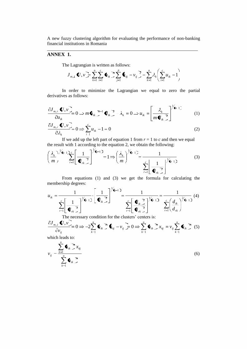
Equations (4) and (5) are derived according to the Annexe no. 1.

When m → 1, the Fuzzy C-Means converges to the Hard C-Means (HCM), and

when we increase its value the partition becomes fuzzier. When m → ∞, then uik →

1/c and the centers tend towards the centroid of the data set (the centers tend to be

equal). The exponent m controls the extent of membership sharing between the

clusters and there is no theoretical basis for an optimal choice for its value.

The algorithm follows the following steps:

- Step 1. Fix c, 2 ≤ c ≤ n, and m, 1 ≤ m ≤ ∞. Initialize(0)

fcU M . Then,

for sth iteration, s = 0, 1, 2, … :

- Step 2. Calculate the c fuzzy cluster centers {vi (s)

} with (5) and U(s)

.

- Step 3. Calculate U(s+1)

using (4) and {vi (s)

}.

- Step 4. Compare U(s+1)

to U(s)

: if ( 1) ( )s sU U stop; otherwise

return to Step 2.

Since the iteration is based on minimizing the objective function, when the

minimum amount of improvement between two iterations is less than ε the process

will stop. One of the main disadvantages of the FCM is its sensitivity to noise and

outliers in data, which may lead to incorrect values for the clusters’ centers.

Several robust methods to deal with noise and outliers have been presented in

Levski (2003).

The FCM algorithm gives the membership degree of every observation for every

cluster iku . The usual criterion to assign the data to their clusters is to choose the

cluster where the observation has the highest membership value. While that may

work for a great number of elements, some other data vectors may be misallocated.

This is the case when the two highest membership degrees are very close to each

other, for example, one observation with a degree of 0.45 for the first cluster and


____________________________________________________________ 0.46 for the third. We call this data vector as “uncertain” observation. Therefore, it

would be useful to introduce in the algorithm some kind of information about the

characteristics of every cluster so that the uncertain observations can be better

allocated depending on which of these features they fulfil more.

III.1. Generation of linguistic variables

When we analyze a group of companies by their financial performances, we have

to be aware of the economic characteristics of the sector they belong to. Levels of

ratios showing theoretical bad performances may indicate, for the specific sector, a

good or average situation for a company. Conversely, a good theoretical value for

the same indicator may indicate a bad evolution of the enterprise in another sector.

Usually, financial analysts use expressions like: “high rate of return”, “low capital

adequacy”, etc. to represent the financial situation of the sector or the company.

Expressions like that can be easily modeled with the use of linguistic variables and

allow the comparison of different financial ratios in a more understandable way

regardless of the sector of activity.

Linguistic variables are quantitative fuzzy variables whose states are fuzzy

numbers that represent linguistic terms, such as very small, medium, and so on

(Klir & Yuan, 1995). In our study we model the eight financial ratios with the help

of eight linguistic variables using five linguistic terms: very low (VL), low (L),

average (A), high (H), very high (VH). To each of the basic linguistic terms we

assign one of five fuzzy numbers, whose membership functions are defined on the

range of the ratios in the data set. It is common to represent linguistic variables

with linguistic terms positioned symmetrically (Lindström, 1998). Since there is no

reason to assume that the empirical distributions of the ratios in our data set are

symmetric, we applied the FCM algorithm to each ratio individually in order to

obtain the fuzzy numbers, which appeared not to be symmetric. Therefore, the

linguistic terms are defined specifically for the sector into consideration. The value

of m was set to 1.5 because it gave a good graphical representation of the fuzzy

numbers, and these were approximated to fuzzy numbers of the trapezoidal form.

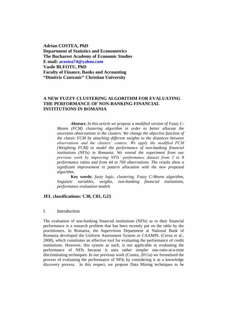
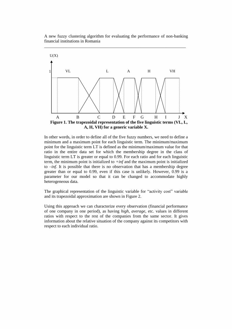
We define the linguistic terms as follows (see Figure 1):

- the linguistic term VL is defined by three points: a minimum point (A),

a maximum point (B) and the minimum point for the linguistic term L

(C);

- the linguistic terms L, A, H are defined by four points: the maximum

point for the previous linguistic term (e.g., point B for the linguistic

term L), a minimum point (e.g., point C for the linguistic term L), a

maximum point (e.g., point D for the linguistic term L) and the

minimum point for the next linguistic term (e.g., point E for the

linguistic term L);

- the linguistic term VH is defined by three points: the maximum point

for the linguistic term H (H), a minimum point (I) and a maximum

point (J).



__________________________________________________________________

A B C D E F G H I J X

Figure 1. The trapezoidal representation of the five linguistic terms (VL, L,

A, H, VH) for a generic variable X.

In other words, in order to define all of the five fuzzy numbers, we need to define a

minimum and a maximum point for each linguistic term. The minimum/maximum

point for the linguistic term LT is defined as the minimum/maximum value for that

ratio in the entire data set for which the membership degree in the class of

linguistic term LT is greater or equal to 0.99. For each ratio and for each linguistic

term, the minimum point is initialized to +inf and the maximum point is initialized

to –inf. It is possible that there is no observation that has a membership degree

greater than or equal to 0.99, even if this case is unlikely. However, 0.99 is a

parameter for our model so that it can be changed to accommodate highly

heterogeneous data.

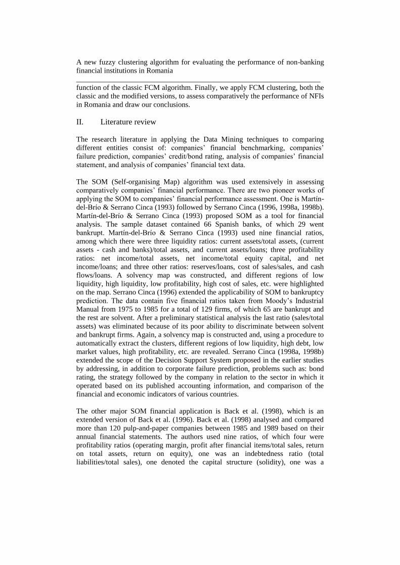
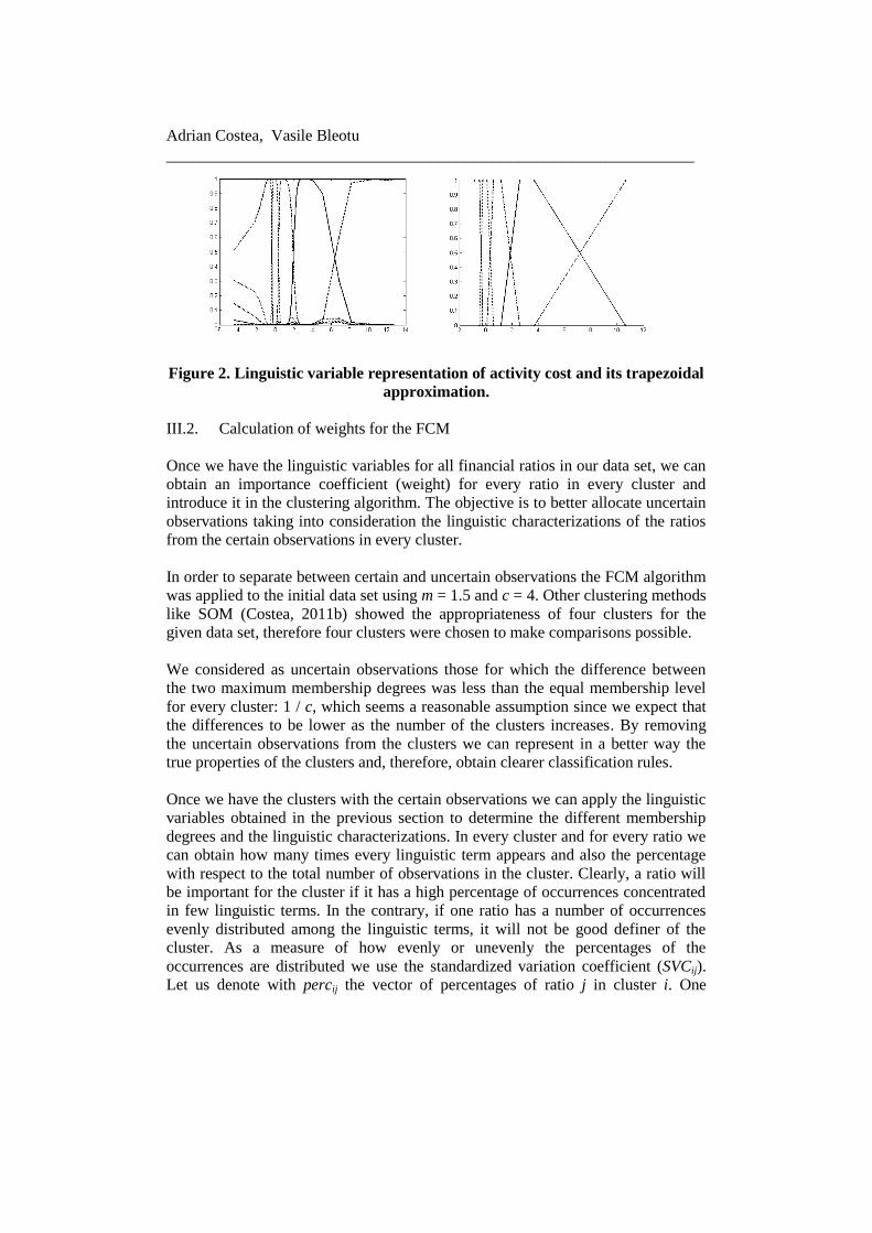
The graphical representation of the linguistic variable for “activity cost” variable

and its trapezoidal approximation are shown in Figure 2.

Using this approach we can characterize every observation (financial performance

of one company in one period), as having high, average, etc. values in different

ratios with respect to the rest of the companies from the same sector. It gives

information about the relative situation of the company against its competitors with

respect to each individual ratio.

VL L A H VH 1

U(X)


____________________________________________________________

Figure 2. Linguistic variable representation of activity cost and its trapezoidal

approximation.

III.2. Calculation of weights for the FCM

Once we have the linguistic variables for all financial ratios in our data set, we can

obtain an importance coefficient (weight) for every ratio in every cluster and

introduce it in the clustering algorithm. The objective is to better allocate uncertain

observations taking into consideration the linguistic characterizations of the ratios

from the certain observations in every cluster.

In order to separate between certain and uncertain observations the FCM algorithm

was applied to the initial data set using m = 1.5 and c = 4. Other clustering methods

like SOM (Costea, 2011b) showed the appropriateness of four clusters for the

given data set, therefore four clusters were chosen to make comparisons possible.

We considered as uncertain observations those for which the difference between

the two maximum membership degrees was less than the equal membership level

for every cluster: 1 / c, which seems a reasonable assumption since we expect that

the differences to be lower as the number of the clusters increases. By removing

the uncertain observations from the clusters we can represent in a better way the

true properties of the clusters and, therefore, obtain clearer classification rules.

Once we have the clusters with the certain observations we can apply the linguistic

variables obtained in the previous section to determine the different membership

degrees and the linguistic characterizations. In every cluster and for every ratio we

can obtain how many times every linguistic term appears and also the percentage

with respect to the total number of observations in the cluster. Clearly, a ratio will

be important for the cluster if it has a high percentage of occurrences concentrated

in few linguistic terms. In the contrary, if one ratio has a number of occurrences

evenly distributed among the linguistic terms, it will not be good definer of the

cluster. As a measure of how evenly or unevenly the percentages of the

occurrences are distributed we use the standardized variation coefficient (SVCij).

Let us denote with percij the vector of percentages of ratio j in cluster i. One



__________________________________________________________________

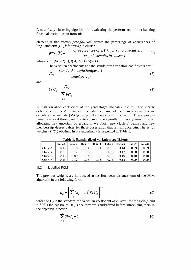
element of this vector, percij(k), will denote the percentage of occurrences of

linguistic term (LT) k for ratio j in cluster i.

_

( )_

ij

nr of occurences of LT k for ratio j incluster iperc k

nr of samples in cluster i (6)

where 1( ),2( ),3( ),4( ),5( )k VL L A H VH .

The variation coefficients and the standardized variation coefficients are:

_ ( )

( )

ij

ij

ij

standard deviation percVC

mean perc (7)

and

1

ij

ij p

ij

j

VCSVC

VC

(8)

A high variation coefficient of the percentages indicates that the ratio clearly

defines the cluster. After we split the data in certain and uncertain observations, we

calculate the weights (SVCij) using only the certain information. These weights

remain constant throughout the iterations of the algorithm. In every iteration, after

allocating new uncertain observations, we obtain new clusters’ centres and new

membership degree values for those observation that remain uncertain. The set of

weights (SVCij) obtained in our experiment is presented in Table 1.

Table 1. Standardized variation coefficients

Ratio 1 Ratio 2 Ratio 3 Ratio 4 Ratio 5 Ratio 6 Ratio 7 Ratio 8

Cluster 1 0.15 0.10 0.14 0.14 0.13 0.14 0.09 0.09

Cluster 2 0.09 0.12 0.16 0.16 0.19 0.12 0.08 0.08

Cluster 3 0.13 0.09 0.14 0.13 0.12 0.19 0.10 0.10

Cluster 4 0.13 0.12 0.13 0.13 0.15 0.15 0.09 0.09

III.3. Modified FCM

The previous weights are introduced in the Euclidean distance term of the FCM

algorithm in the following form:

1/ 2

2

1

( )p

ik kj ij ij

j

d x v SVC (9)

where SVCij is the standardized variation coefficient of cluster i for the ratio j, and

it fulfils the constraint (10) since they are standardized before introducing them in

the objective function.

1

1p

ij

j

SVC (10)


____________________________________________________________

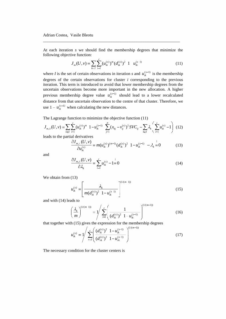
At each iteration s we should find the membership degrees that minimize the

following objective function:

( ) ( ) 2 ( 1)

1

( , ) ( ) ( ) 1c

s m s s

m ik ik ik

k I i

J U v u d u (11)

where I is the set of certain observations in iteration s and ( 1)s

iku is the membership

degrees of the certain observations for cluster i corresponding to the previous

iteration. This term is introduced to avoid that lower membership degrees from the

uncertain observations become more important in the new allocation. A higher

previous membership degree value ( 1)s

iku should lead to a lower recalculated

distance from that uncertain observation to the centre of that cluster. Therefore, we

use 1 – ( 1)s

iku when calculating the new distances.

The Lagrange function to minimize the objective function (11)

( ) ( 1) ( ) 2 ( )

,

1 1 1

( , ) ( ) 1 ( ) 1pc c

s m s s s

m ik ik kj ij ij k ik

k I i j k I i

J U v u u x v SVC u (12)

leads to the partial derivatives !

, ( ) ( 1) ( ) 2 ( 1)

( )

( , )( ) ( ) 1 0

m s m s s

ik ik ik ks

ik

J U vm u d u

u (13)

and !

, ( )

1

( , )1 0

cm s

ik

ik

J U vu (14)

We obtain from (13) (1/( 1))

( )

( ) 2 ( 1)( ) 1

m

s kik s s

ik ik

um d u

(15)

and with (14) leads to (1/( 1))

(1/( 1))

( ) 2 ( 1)1

11

( ) 1

mm c

k

s si ik ik

m d u (16)

that together with (15) gives the expression for the membership degrees (1/( 1))

( ) 2 ( 1)

( )

( ) 2 ( 1)1

( ) 11

( ) 1

ms s

cik iks

ik s sr rk rk

d uu

d u (17)

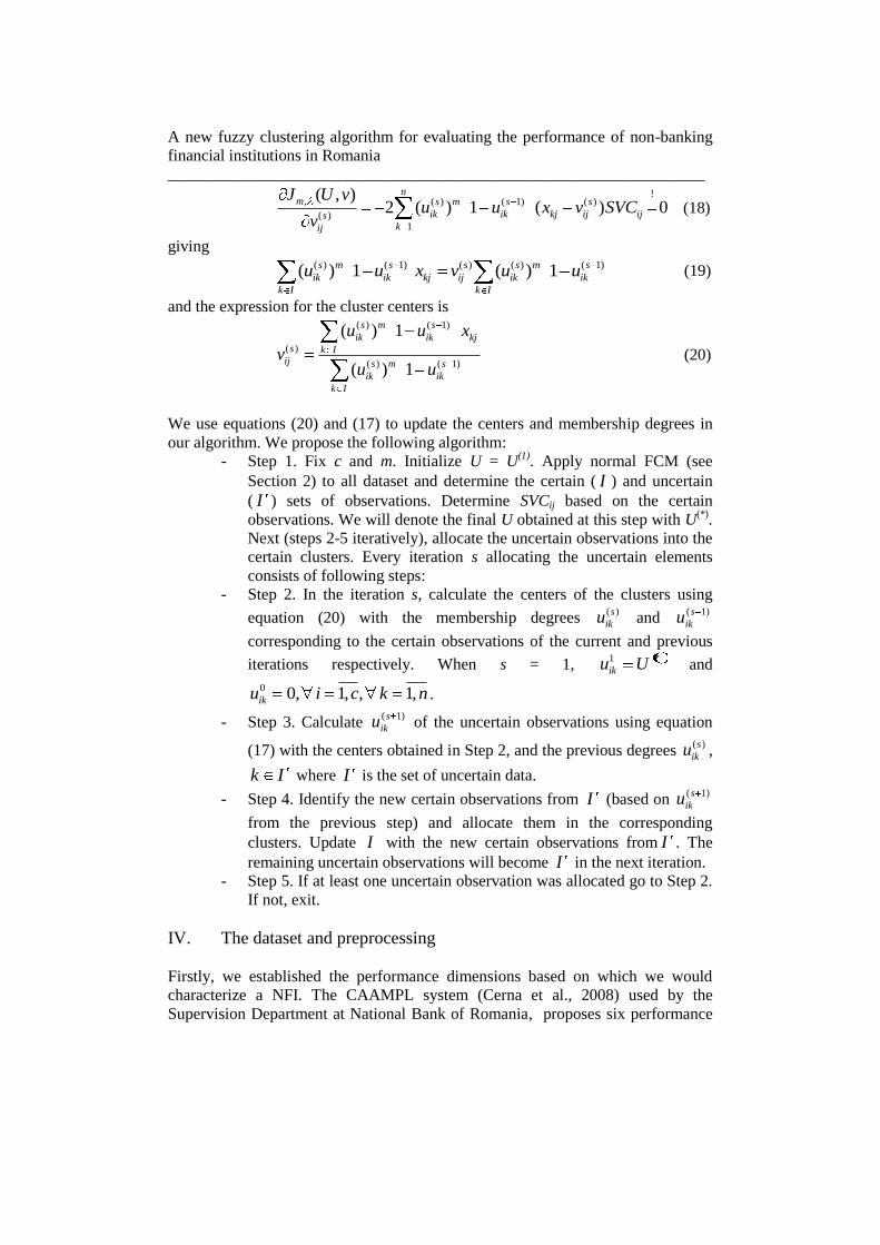
The necessary condition for the cluster centers is



__________________________________________________________________ !

, ( ) ( 1) ( )

( )1

( , )2 ( ) 1 ( ) 0

nm s m s s

ik ik kj ij ijskij

J U vu u x v SVC

v (18)

giving ( ) ( 1) ( ) ( ) ( 1)( ) 1 ( ) 1s m s s s m s

ik ik kj ij ik ik

k I k I

u u x v u u (19)

and the expression for the cluster centers is ( ) ( 1)

( )

( ) ( 1)

( ) 1

( ) 1

s m s

ik ik kjs k I

ij s m s

ik ik

k I

u u x

vu u

(20)

We use equations (20) and (17) to update the centers and membership degrees in

our algorithm. We propose the following algorithm:

- Step 1. Fix c and m. Initialize U = U(1)

. Apply normal FCM (see

Section 2) to all dataset and determine the certain ( I ) and uncertain

( I ) sets of observations. Determine SVCij based on the certain

observations. We will denote the final U obtained at this step with U(*)

.

Next (steps 2-5 iteratively), allocate the uncertain observations into the

certain clusters. Every iteration s allocating the uncertain elements

consists of following steps:

- Step 2. In the iteration s, calculate the centers of the clusters using

equation (20) with the membership degrees ( )s

iku and ( 1)s

iku

corresponding to the certain observations of the current and previous

iterations respectively. When s = 1, *1 Uuik and

0 0, 1, , 1,iku i c k n .

- Step 3. Calculate ( 1)s

iku of the uncertain observations using equation

(17) with the centers obtained in Step 2, and the previous degrees ( )s

iku ,

k I where I is the set of uncertain data.

- Step 4. Identify the new certain observations from I (based on ( 1)s

iku

from the previous step) and allocate them in the corresponding

clusters. Update I with the new certain observations from I . The

remaining uncertain observations will become I in the next iteration.

- Step 5. If at least one uncertain observation was allocated go to Step 2.

If not, exit.

IV. The dataset and preprocessing

Firstly, we established the performance dimensions based on which we would

characterize a NFI. The CAAMPL system (Cerna et al., 2008) used by the

Supervision Department at National Bank of Romania, proposes six performance


____________________________________________________________ dimensions to evaluate the performance of credit institutions: capital adequacy (C),

quality of ownership (A), assets’ quality (A), management (M), profitability (P),

liquidity (L). The CAAMPL system uses the financial reports of credit institutions

and evaluates these six components. The six dimensions are rated using a 1 to 5

scale, where 1 represents best performance and 5 the worst. Four dimensions

(capital adequacy, assets’ quality, profitability, and liquidity) are quantitative

dimensions and are evaluated based on a number of indicators. The other two

dimensions are qualitative dimensions, evaluated on the textual information

provided by the banks as legal reporting requirements at the time of their

authorization or as a consequence of changes in their situation. These two

dimensions can also be evaluated from the information obtained during on-site

inspections. Finally, a composite rating is calculated as a weighted average of the

dimensions’ ratings.

In our research regarding the NFIs’ sector, we restrict the number of the

performance dimensions to three quantitative dimensions, namely: capital

adequacy (C), assets’ quality (A) and profitability (P). The other quantitative

dimension used in evaluating the credit institutions (liquidity dimension) is not

applicable to NFIs, since they do not attract retail deposits. We have also

eliminated the qualitative dimensions from our experiment (quality of ownership

and management) because they involve a distinct approach and it was not the scope

of this study to take them into account.

After choosing the performance dimensions, we select different indicators for each

dimension based on the analysis of the periodic financial statements of the NFIs.

We select the following indicators for assessing the degree of capitalization:

1) Equity ratio = own capital / total assets (net value) – Leverage

2) Own capital / equity – OC_to_EQ

3) Indebtedness sources = borrowings / own capital – BOR_to_OC

The evaluation of the assets’ quality of NFIs is generally based on the value of

loans granted, as well as on the value of nonperforming loans. The set of indicators

for assessing the assets’ quality is as follows:

1) Loans granted to clients (net value) / total assets (net value) – Loans_to_Assets

2) Loans granted to clients (net value) / total borrowings – Loans_to_BOR

3) Past due and doubtful loans (net value) / total loans portfolio (net value) –

PDDL_to_Loans

4) Past due and doubtful claims (net value) / total assets (net value) –

PDDC_to_Assets

5) Past due and doubtful claims (net value) / own capital – PDDC_to_OC

Profitability is measured by classical indicators, namely:

1) Return on assets = net income / total assets (net value) – ROA

2) Return on equity = net profit / own capital – ROE

3) The rate of profit = gross profit / total revenues – GP_to_REV

4) Activity cost = total costs / total revenues – Costs_to_REV



__________________________________________________________________

The next step in building our data set is to chose the NFIs, the period and the

periodicity for which we would calculate the ratios. We chose the NFIs that are

entered in the Special register, for the period 2007-2010, by quarter. In general,

NFIs in Romania are included in three registers: Evidence register, General register

and Special register. Except pawn shops and credit unions which are included in

the Evidence register, other NFIs are entered in the General register. The Special

register includes only those NFIs from the General register that meet certain

criteria of performance in terms of loans and borrowings. NFIs that meet these

criteria three reporting-periods in a row (three quarters) are entered in the Special

register. Conversely, if a NFI from the Special register does not satisfy the criteria

three consecutive quarters is re-entered in the General register. In total, in the

analyzed period, there were 65 active NFIs in the Special register. We collected the

data for these 65 NFIs quarterly from 2007 to 2010, obtaining a total of 769

observations. Then, we calculated the above twelve financial ratios. We discarded

four ratios (Leverage – for the capital adequacy dimension, Loans_to_Assets and

Loans_to_BOR – for the assets’ quality dimension and ROA – for profitability

dimension) from our analysis due to high variation of their values/incorrect values

remaining with eight ratios. Also, the 769 observations x 8 ratios data set contains

quarterly and yearly averages (16 quarterly averages and 4 yearly averages = 20

observations).

We preprocessed our data set by leveling the outliers to the interval [-50, 50] and

then, by normalizing each ratio (subtracting from each value the mean and dividing

the result to the standard deviation of that ratio). We have done this in order to

avoid that our algorithm places to much importance to the extreme values.

V. The experiment

We have applied the FCM algorithm and its modified version to our dataset trying

to find clusters with similar performance. The implementation has been done using

Matlab environment by building a script based on the existing functions.

We have used m = 1.5 in the implementation of the algorithm as we have done

when we have generated the linguistic variables, and c = 4 to make the results

comparable with those from our previous work (Costea, 2011b) when we applied

the SOM algorithm. We have characterized each cluster by using the linguistic

variables (see Table 2).

We considered that one linguistic term characterizes one cluster if it represents

more than 40% out of total number of samples for that cluster. We chose 40% in

order to allow maximum two linguistic term to characterize a cluster for each ratio.

For example, for cluster 1, and ratio OC_to_EQ, we have one linguistic terms that

has more than 40% of the occurrences (A). When all linguistic terms for one

cluster and one ratio are under 40% we say that the ratio is not a good definer for


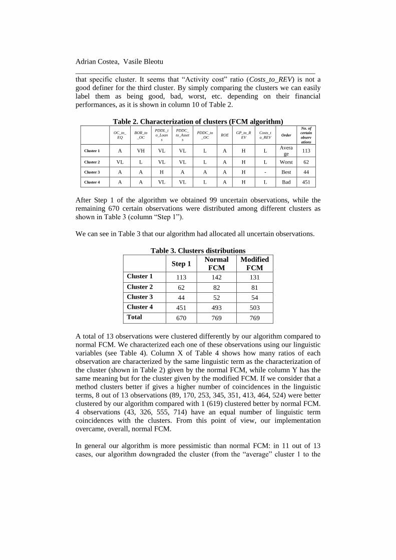
____________________________________________________________ that specific cluster. It seems that “Activity cost” ratio (Costs_to_REV) is not a

good definer for the third cluster. By simply comparing the clusters we can easily

label them as being good, bad, worst, etc. depending on their financial

performances, as it is shown in column 10 of Table 2.

Table 2. Characterization of clusters (FCM algorithm)

OC_to_

EQ

BOR_to

_OC

PDDL_t

o_Loan

s

PDDC_

to_Asset

s

PDDC_to

_OC ROE

GP_to_R

EV

Costs_t

o_REV Order

No. of

certain

observ

ations

Cluster 1 A VH VL VL L A H L Avera

ge 113

Cluster 2 VL L VL VL L A H L Worst 62

Cluster 3 A A H A A A H - Best 44

Cluster 4 A A VL VL L A H L Bad 451

After Step 1 of the algorithm we obtained 99 uncertain observations, while the

remaining 670 certain observations were distributed among different clusters as

shown in Table 3 (column “Step 1”).

We can see in Table 3 that our algorithm had allocated all uncertain observations.

Table 3. Clusters distributions

Step 1

Normal

FCM

Modified

FCM Cluster 1 113 142 131

Cluster 2 62 82 81

Cluster 3 44 52 54

Cluster 4 451 493 503

Total 670 769 769

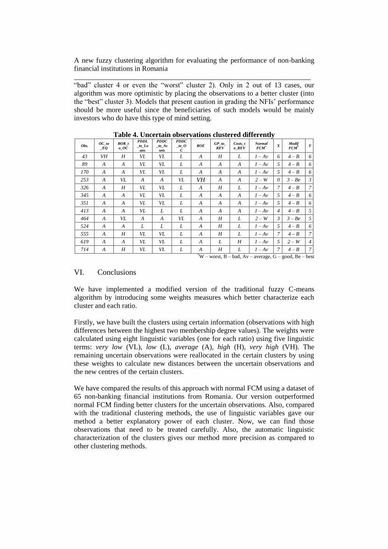
A total of 13 observations were clustered differently by our algorithm compared to

normal FCM. We characterized each one of these observations using our linguistic

variables (see Table 4). Column X of Table 4 shows how many ratios of each

observation are characterized by the same linguistic term as the characterization of

the cluster (shown in Table 2) given by the normal FCM, while column Y has the

same meaning but for the cluster given by the modified FCM. If we consider that a

method clusters better if gives a higher number of coincidences in the linguistic

terms, 8 out of 13 observations (89, 170, 253, 345, 351, 413, 464, 524) were better

clustered by our algorithm compared with 1 (619) clustered better by normal FCM.

4 observations (43, 326, 555, 714) have an equal number of linguistic term

coincidences with the clusters. From this point of view, our implementation

overcame, overall, normal FCM.

In general our algorithm is more pessimistic than normal FCM: in 11 out of 13

cases, our algorithm downgraded the cluster (from the “average” cluster 1 to the



__________________________________________________________________

“bad” cluster 4 or even the “worst” cluster 2). Only in 2 out of 13 cases, our

algorithm was more optimistic by placing the observations to a better cluster (into

the “best” cluster 3). Models that present caution in grading the NFIs’ performance

should be more useful since the beneficiaries of such models would be mainly

investors who do have this type of mind setting.

Table 4. Uncertain observations clustered differently

Obs. OC_to

_EQ

BOR_t

o_OC

PDDL

_to_Lo

ans

PDDC

_to_As

sets

PDDC

_to_O

C

ROE GP_to_

REV

Costs_t

o_REV

Normal

FCM* X Modif

FCM* Y

43 VH H VL VL L A H L 1 – Av 6 4 – B 6

89 A A VL VL L A A A 1 – Av 5 4 – B 6

170 A A VL VL L A A A 1 – Av 5 4 – B 6

253 A VL A A VL VH A A 2 – W 0 3 – Be 3

326 A H VL VL L A H L 1 – Av 7 4 – B 7

345 A A VL VL L A A A 1 – Av 5 4 – B 6

351 A A VL VL L A A A 1 – Av 5 4 – B 6

413 A A VL L L A A A 1 – Av 4 4 – B 5

464 A VL A A VL A H L 2 – W 3 3 – Be 5

524 A A L L L A H L 1 – Av 5 4 – B 6

555 A H VL VL L A H L 1 – Av 7 4 – B 7

619 A A VL VL L A L H 1 – Av 5 2 – W 4

714 A H VL VL L A H L 1 – Av 7 4 – B 7 *W – worst, B – bad, Av – average, G – good, Be – best

VI. Conclusions

We have implemented a modified version of the traditional fuzzy C-means

algorithm by introducing some weights measures which better characterize each

cluster and each ratio.

Firstly, we have built the clusters using certain information (observations with high

differences between the highest two membership degree values). The weights were

calculated using eight linguistic variables (one for each ratio) using five linguistic

terms: very low (VL), low (L), average (A), high (H), very high (VH). The

remaining uncertain observations were reallocated in the certain clusters by using

these weights to calculate new distances between the uncertain observations and

the new centres of the certain clusters.

We have compared the results of this approach with normal FCM using a dataset of

65 non-banking financial institutions from Romania. Our version outperformed

normal FCM finding better clusters for the uncertain observations. Also, compared

with the traditional clustering methods, the use of linguistic variables gave our

method a better explanatory power of each cluster. Now, we can find those

observations that need to be treated carefully. Also, the automatic linguistic

characterization of the clusters gives our method more precision as compared to

other clustering methods.


____________________________________________________________

Acknowledgements

This work was supported from the European Social Fund through Sectoral

Operational Programme Human Resources Development 2007-2013, project

number POSDRU/89/1.5/S/59184 „Performance and excellence in postdoctoral

research in Romanian economics science domain”.

REFERENCES

[1] Altman, E. I. (1968), Financial Ratios, Discriminant Analysis and the

Prediction of Corporate Bankruptcy. The Journal of Finance, 23, 589-609;

[2] Back, B., Sere, K., and Vanharanta, H. (1996, August 20-23), Data

Mining Accounting Numbers Using Self-organising Maps. Proceedings

from Finnish Artificial Intelligence Conference. Finland: Vaasa;

[3] Back, B., Sere, K., and Vanharanta, H. (1998), Managing Complexity in

Large Databases Using Self-organizing Maps. Accounting Management and

Information Technologies, 8(4), 191-210;

[4] Back, B., Toivonen, J., Vanharanta, H., and Visa, A. (2001), Comparing

Numerical Data and Text Information from Annual Reports Using Self-

organizing Maps. International Journal of Accounting Information Systems,

2(4), 249-269;

[5] Baležentis, A. and Baležentis, T. (2011), A Novel Method for Group Multi-

attribute Decision Making with Two-tuple Linguistic Computing: Supplier

Evaluation under Uncertainty. ECECSR , ASE Publishing, 45(4): 5-30;

[6] Bezdek, J.C. (1981), Pattern Recognition with Fuzzy Objective Function

Algorithms. Plenum Press, New York, 1981;

[7] Cerna, S., Donath, L., Seulean, V., Herbei, M., Bărglăzan, D., Albulescu,

C. and Boldea, B. (2008), Financial Stability. West University Publishing

House, Timişoara, Romania, 2008;

[8] Coakley, J. R., and Brown, C. E. (2000), Artificial Neural Networks in

Accounting and Finance: Modelling Issues. International Journal of

Intelligent Systems in Accounting, Finance & Management, 9, 119-144;

[9] Costea, A. (2011a), The Process of Knowledge Discovery in Databases

(KDD) - A Framework for Assessing the Performance of Non-banking

Financial Institutions; Proceedings of the 10th International Conference of

Informatics in Economy (IE2011), 5-7 May 2011, Academy of Economic

Studies, Bucuresti, Organizers: Economy in Informatics Department, Faculty

of C.S.I.E. and INFOREC Association, CD-ROM version ISSN 2247-1480,

ISSN-L 2247-1480, section: Information & Communication Technology,

position 32, 6 pages;

[10] Costea, A. (2011b), Performance Benchmarking of Non-banking Financial

Institutions by means of Self-Organising Map Algorithm; accepted for

publication in East-West Journal of Economics and Business (ISSN 1108-



__________________________________________________________________

2992). The paper has been presented to the 2nd International Conference on

International Business (ICIB 2011), organized by the Department of

International and European Studies, University of Macedonia, Thessaloniki,

Greece, European Center for the Development of Vocational Training,

Thessaloniki, Greece, Faculty of Political Science, University of Messina,

Messina Italy and CRIISEA, University of Picardie, Amiens, France, 19-21

May, Thessaloniki, Greece;

[11] De Andres, J. (2001), Statistical Techniques vs. SEES Algorithm. An

Application to a Small Business Environment. The International Journal of

Digital Accounting Research, 1(2), 153-178;

[12] Drobics, M., Winiwarter, W., and Bodenhofer, U. (2000), Interpretation of

Self-Organizing Maps with Fuzzy Rules. Proceedings of the ICTA 2000 –

The Twelfth IEEE International Conference on Tools with Artificial

Intelligence, Vancouver;

[13] Eklund, T., Back, B., Vanharanta, H., and Visa, A. (2003), Financial

Benchmarking Using Self-organizing Maps—Studying the International

Pulp and Paper Industry. In J. Wang (Ed.), Data Mining—Opportunities and

Challenges (Chapter 14, pp. 323-349). Hershey, P.A.: Idea Group Publishing;

[14] Jain, A. K., Murty, M.N., and Flynn, P.J. (1999, September), Data

Clustering: A Review . ACM Computing Survey, vol. 31, no. 3;

[15] Karlsson, J., Back, B., Vanharanta, H., and Visa, A. (2001, February),

Financial Benchmarking of Telecommunications Companies. TUCS

Technical Report No. 395;

[16] Klir, G.J. and Yuan, B. (1995), Fuzzy Sets and Fuzzy Logic. Theory and

Applications. Prentice Hall PTR, Upper Saddle River, New Jersey;

[17] Kloptchenko, A. (2003), Text Mining Based on the Prototype Matching

Method. TUCS Ph.D Dissertation, Abo Akademi University, Turku, Finland;

[18] Kloptchenko, A., Eklund, T., Karlsson, J., Back, B., Vanharanta, H., and

Visa A. (2004), Combining Data and Text Mining Techniques for

Analysing Financial Reports. International Journal of Intelligent Systems in

Accounting, Finance and Management, 12(1), 29-41;

[19] Koskivaara, E. (2004), Artificial Neural Networks in Analytical Review

Procedures. Managerial Auditing Journal, 19(2), 191-223;

[20] Leski, J., (2003), Towards a Robust Fuzzy Clustering. Fuzzy Sets and

System 137, pp. 215–233;

[21] Lindholm, C.K. and Liu, S. (2003), Fuzzy Clustering Analysis of the Early

Warning Signs of Financial Crisis; Proceedings of the FIP2003, an

International Conference on Fuzzy Information Processing: Theory and

Applications, Beijing, March 1–4;

[22] Lindström, T. (1998), A Fuzzy Design of the Willingness to Invest in

Sweden. Journal of Economic Behavior and Organization, vol. 36, pp. 1–17;

[23] Martín-del-Brío, B., and Serrano Cinca, C. (1993), Self-organizing Neural

Networks for the Analysis and Representation of Data: Some Financial

Cases. Neural Computing & Applications, 1(2), 193-206;


____________________________________________________________ [24] O’Leary, D. E. (1998), Using Neural Networks to Predict Corporate

Failure. International Journal of Intelligent Systems in Accounting, Finance

& Management, 7, 187-197;

[25] Ohlson, J. A. (1980), Financial Ratios and the Probabilistic Prediction of

Bankruptcy. Journal of Accounting Research, 18(1), 109-131;

[26] Ong, J. and Abidi, S. S. R. (1999, June 28-July 1), Data Mining Using

Self-Organizing Kohonen Maps: A Technique for Effective Data Clustering

& Visualisation. Proceedings from International Conference on Artificial

Intelligence (IC-AI’99). Las Vegas;

[27] Pele, D.T. (2011, March 30), Information Entropy and Occurence of

Extreme Negative Returns. Journal of Applied Quantitative Methods, 6(1),

ISSN 1842-4562;

[28] Serrano Cinca, C. (1996), Self-organizing Neural Networks for Financial

Diagnosis. Decision Support Systems, 17, 227-238;

[29] Serrano Cinca, C. (1998a), Self-organizing Maps for Initial Data Analysis:

Let Financial Data Speak for themselves. In G. Deboeck and T. Kohonen

(Eds.), Visual Intelligence in Finance Using Self-organizing Maps. Springer

Verlag;

[30] Serrano Cinca, C. (1998b), From Financial Information to Strategic

Groups—A self-organizing Neural Network Approach. Journal of

Forecasting, 17, 415-428;

[31] Shirata, C. Y. (2001, October 28-31), The Relationship between Business

Failure and Decision Making by Manager: Empirical Analysis. Proceedings

from 13th Asian-Pacific Conference on International Accounting Issues. Rio

de Janeiro, Brazil;

[32] Toivonen, J., Visa, A., Vesanen, T., Back, B., and Vanharanta, H. (2001),

Validation of Text Clustering Based on Document Contents. Machine

Learning and Data Mining in Pattern Recognition (MLDM 2001). Leipzig,

Germany;

[33] Vesanto, J. and Alhoniemi, E. (2000), Clustering of the Self-organizing

Map. IEEE Transactions on Neural Networks, 11(3), 586-600;

[34] Visa, A., Toivonen, J., Back, B., and Vanharanta, H. (2002), Contents

Matching Defined by Prototypes: Methodology Verification with Books of

the Bible. Journal of Management Information Systems, 18(4), 87-100;

[35] Voineagu, V., Sacală, M.D. and Sacală, I.Ş. (2011), Technical Analysis and

Econometric Prediction Using Wave Refraction Method. ECECSR , ASE

Publishing, 45(3): 5-24;

[36] Wang, J.W., Cheng, C.H., and Huang, K.C. (2009), Fuzzy Hierarchical

TOPSIS for Supplier Selection. Applied Soft Computing 9(1), 377–386.



__________________________________________________________________

ANNEX 1.

The Lagrangian is written as follows: n

k

c

i

ikk

n

k

c

i

p

j

ijkj

m

ikm uvxuvUJ1 11 1 1

2

, 1,

In order to minimize the Lagrangian we equal to zero the partial

derivatives as follows:

11

2

21,00

, m

ik

kikkik

m

ik

ik

m

dmudum

u

vUJ (1)

010,

1

,c

i

ik

k

mu

vUJ (2)

If we add up the left part of equation 1 from r = 1 to c and then we equal

the result with 1 according to the equation 2, we obtain the following:

c

r

m

rk

mk

c

r

m

rk

mk

d

mdm

1

11

2

11

1

11

2

11

1

11

1 (3)

From equations (1) and (3) we get the formula for calculating the

membership degrees:

c

r

m

rk

ikc

r

m

rk

ik

m

ikc

r

m

rk

ik

d

d

d

dd

d

u

1

12

1

11

2

2

11

2

1

11

2

111

1

1 (4)

The necessary condition for the clusters’ centers is: n

k

m

ikij

n

k

kj

m

ik

n

k

ijkj

m

ik

ij

muvxuvxu

v

vUJ

111

,020

, (5)

which leads to:

n

k

m

ik

n

k

kj

m

ik

ij

u

xu

v

1

1 (6)

adrian costea, phd department of statistics and econometrics vasile … costea (t).pdf ·...

Documents