advanced computation for complex...

Advanced Computation for Complex Materials

• Computational Progress is brainpower limited, not machine limited– Algorithms– Physics

• Major progress in algorithms– Quantum Monte Carlo– Density Matrix Renormalization Group

• Building the right Hamiltonians• Solving the dimensionality/sign problem

Getting started: density functional theory

• “DFT is exact” is a silly statement.

• LDA and LDA++ are clever, useful calculation schemes– Always useful for getting started with a new material– Maybe all that’s needed for weakly correlated systems

– Maybe all you can do for complex structures– The Wrong Framework for strongly correlated systems

• Strong interatomic correlations not treated

• Hybrids (LDA+DMFT) useful in some cases

• Many systems require reduction to a model: the correlations are too complicated.

• Getting the model:– The past: educated, insightful guesswork...

– The future: systematic reduction from band structure?

Solving lattice models• Direct attack (exact diagonalization): Exponential growth of

effort with system size– Going from workstation to supercomputer only buys you a few more

sites

• Clever algorithms: beating the exponential– Quantum Monte Carlo

• Determinantal

• World line, stochastic series expansions: loop algorithms!

– Density matrix renormalization group

• History of previous advances:– An improved algorithm allows a new class of problems or new regime

to be solved– Trying to go beyond the regime runs into exponential problems.

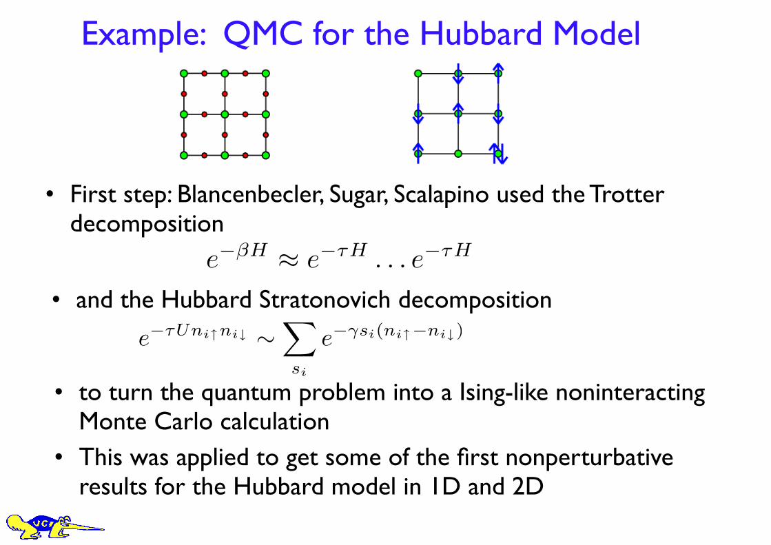
Example: QMC for the Hubbard Model

• First step: Blancenbecler, Sugar, Scalapino used the Trotter decomposition

• to turn the quantum problem into a Ising-like noninteracting Monte Carlo calculation

• This was applied to get some of the first nonperturbative results for the Hubbard model in 1D and 2D

e!!H ! e!"H . . . e!"H

• and the Hubbard Stratonovich decomposition

e!!Uni!ni" !!

si

e!"si(ni!!ni")

Example: QMC for the Hubbard Model (cont)• First problem: for β >~ 4, a numerical instability ruined the

simulation, requiring quadruple precision• Solution: we found a matrix factorization procedure that cured

the instability at all β• Second problem: once we could go to lower temperatures, we

encountered the fermion sign problem ( β ~ 6) away from half filling.– Universal problem related to Fermi statistics– Problem is in treating a nonpositive quantity as a probability– Simulations still possible (use |P|) but get exponentially hard

as <sign(P)> vanishes• All QMC methods still suffer the sign problem, but some

approximate treatments have emerged (constrain sign with approximate wavefunction).

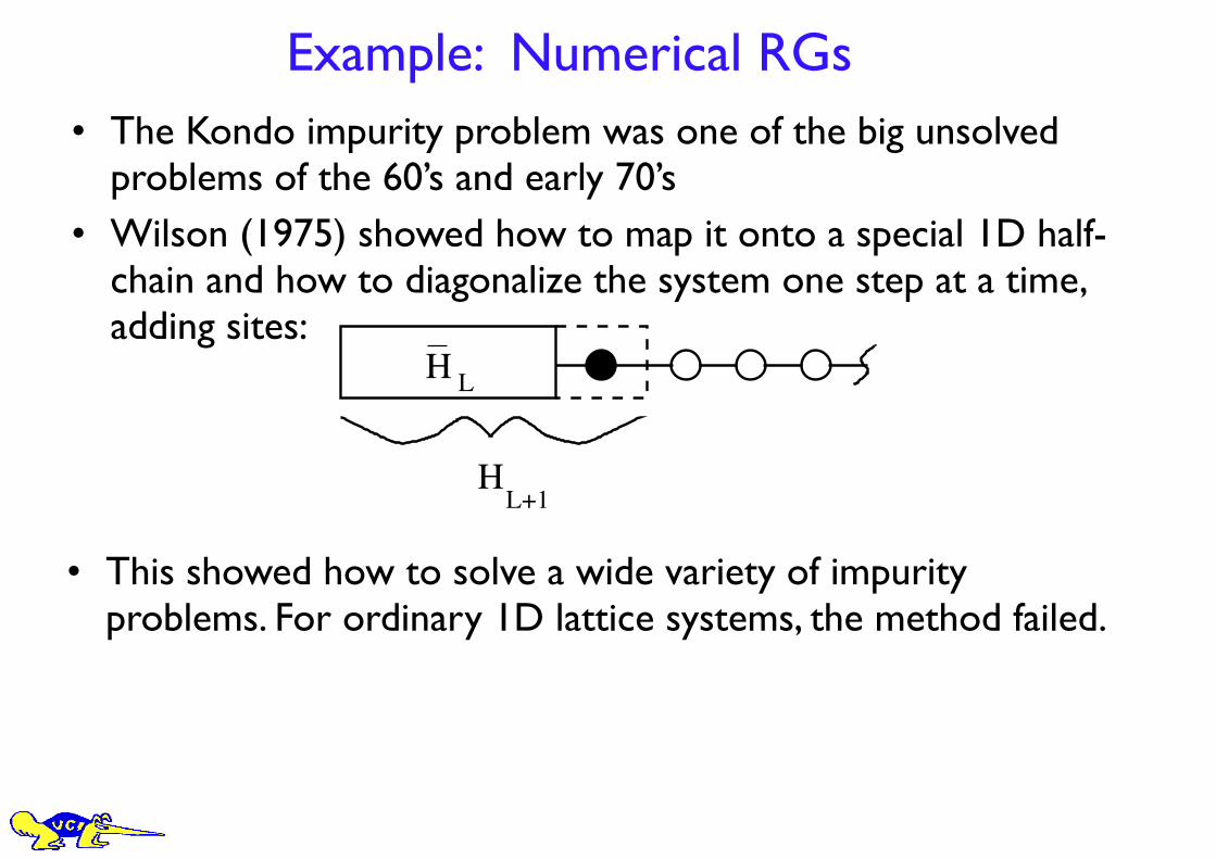
Example: Numerical RGs• The Kondo impurity problem was one of the big unsolved

problems of the 60’s and early 70’s• Wilson (1975) showed how to map it onto a special 1D half-

chain and how to diagonalize the system one step at a time, adding sites:

H

H

L

L+1

• This showed how to solve a wide variety of impurity problems. For ordinary 1D lattice systems, the method failed.

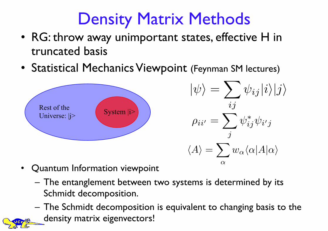
Density Matrix Methods• RG: throw away unimportant states, effective H in

truncated basis• Statistical Mechanics Viewpoint (Feynman SM lectures)

• Quantum Information viewpoint

– The entanglement between two systems is determined by its Schmidt decomposition.

– The Schmidt decomposition is equivalent to changing basis to the density matrix eigenvectors!

Rest of the Universe: |j> System |i>

Density Matrices—Review

Reference: R.P. Feynman, Statistical Mechanics: A Set ofLectures

Let |i! be the states of the block (the system), and |j! bethe states of the rest of the lattice (the rest of the universe).If ! is a state of the entire lattice,

|!! =!

ij

!ij |i!|j!

The density matrix is

"ii! =!

j

!!

ij!i!j

If operator A acts only on the system,

"A! =!

ii!

Aii!"i!i = Tr"A

Let " have eigenstates |v!! and eigenvalues w! # 0("

! w! = 1). Then

"A! =!

!

w!"v!|A|v!!

If for a particular #, w! $ 0, we make no error in "A! if wediscard |v!!. One can also show we make no error in !.

If the rest of the universe is regarded as a “heat bath” atinverse temperature $ to which the system is weakly cou-pled,

" =1

Zexp(%$H).

In this case the eigenstates of " are the eigenstates of H.




|!! =!

ij

!ij |i!|j!


"ii! =!

j

!!

ij!i!j


"A! =!

ii!

Aii!"i!i = Tr"A


! w! = 1). Then

"A! =!

!

w!"v!|A|v!!



" =1

Zexp(%$H).





|!! =!

ij

!ij |i!|j!


"ii! =!

j

!!

ij!i!j


"A! =!

ii!

Aii!"i!i = Tr"A


! w! = 1). Then

"A! =!

!

w!"#|A|#!



" =1

Zexp(%$H).


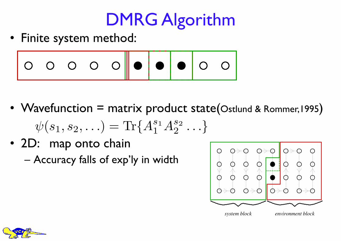
DMRG Algorithm• Finite system method:

• Wavefunction = matrix product state(Ostlund & Rommer,1995)

• 2D: map onto chain– Accuracy falls of exp’ly in width

!(s1, s2, . . .) = Tr{As11 As2

2 . . .}

Extensions – 2D and Fermion Systems

(Noack, White, Scalapino, 1994)

system block environment block

• 1D algorithm “folded” into 2D• finite system algorithm necessary

• convergence depends strongly on width of system! exponential in width for spinless fermions (Liang & Pang 1994)

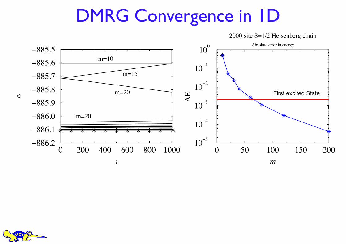
DMRG Convergence in 1D

0 200 400 600 800 1000i

!886.2!886.1!886.0!885.9!885.8!885.7!885.6!885.5

E

m=10

m=15

m=20

m=20

0 50 100 150 200m

10!5

10!4

10!3

10!2

10!1

100

!"

2000 site S=1/2 Heisenberg chainAbsolute error in energy

First excited State

DMRG--doped “2D” systems

0.35

0.25

12 x 8 system, Vertical PBC’sJx/t= 0.55,Jy/t=0.45, mu=1.165,doping=0.1579

-0.04 0.04

12 x 8 system, Vertical PBC’sJx/t= 0.55,Jy/t=0.45, mu=1.165,doping=0.1579

Stripes Local pairing along stripes

Triangular Lattice

• Only one sublattice pinned, other two rotate in a cone• Other two have z component -M/2• Here only have L = 3, 6, 9, ...

0.35

17.3 x 9 lattice

Pinning fields

<S >z

y

DMRG, QMC: Status as of ~2000• 2D Unfrustrated spin systems:

– QMC improvements (loop algorithm!) enable huge systems, high accuracy

• 2D Fermions:– DMRG: very accurate on ladders, accuracy falls of exp’ly

with width, still useful up to ~16x8 t-J clusters– QMC: Improvements in methods and variational

wavefunctions give excellent results– But: still disagreements on pairing versus stripe/CDWs in

key models: materials chaos!

• Dynamics: very limited!

DMRG: New developments• Quantum Information: Major new ideas for DMRG!

– Key people: Vidal, Verstraete, Cirac– Time evolution, even far from equilibrium– Finite temperature, disorder, periodic boundaries– New 2D “PEPS” method: linear scaling in width, all

exponential scaling gone!• Unfortunately, on current computers, still more efficient to use

older mapping to 1D DMRG.

• Why has QI been so successful?– They think about evolution of quantum states.– They introduce auxiliary systems to manage entanglement.– Many clever mathematical tricks.

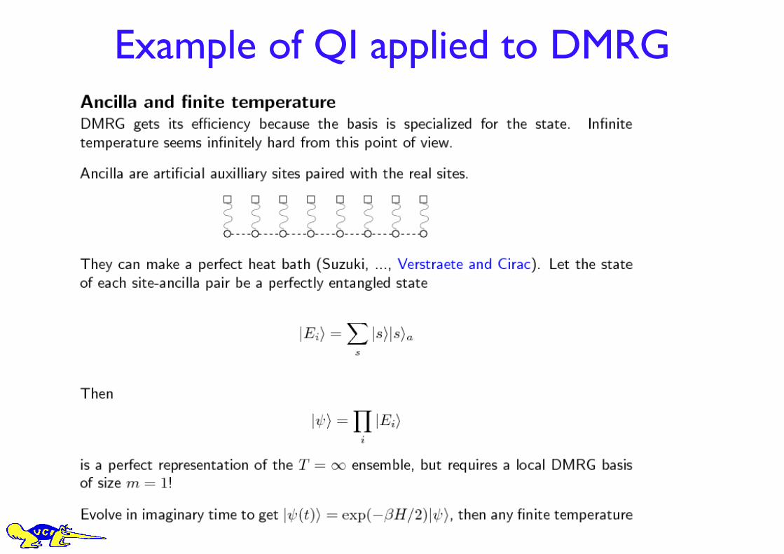
Example of QI applied to DMRG

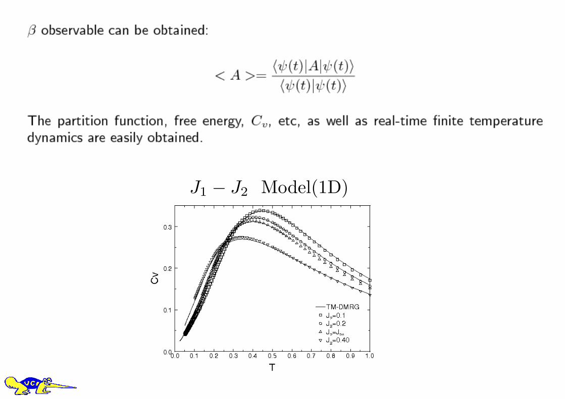
J1 ! J2 Model(1D)

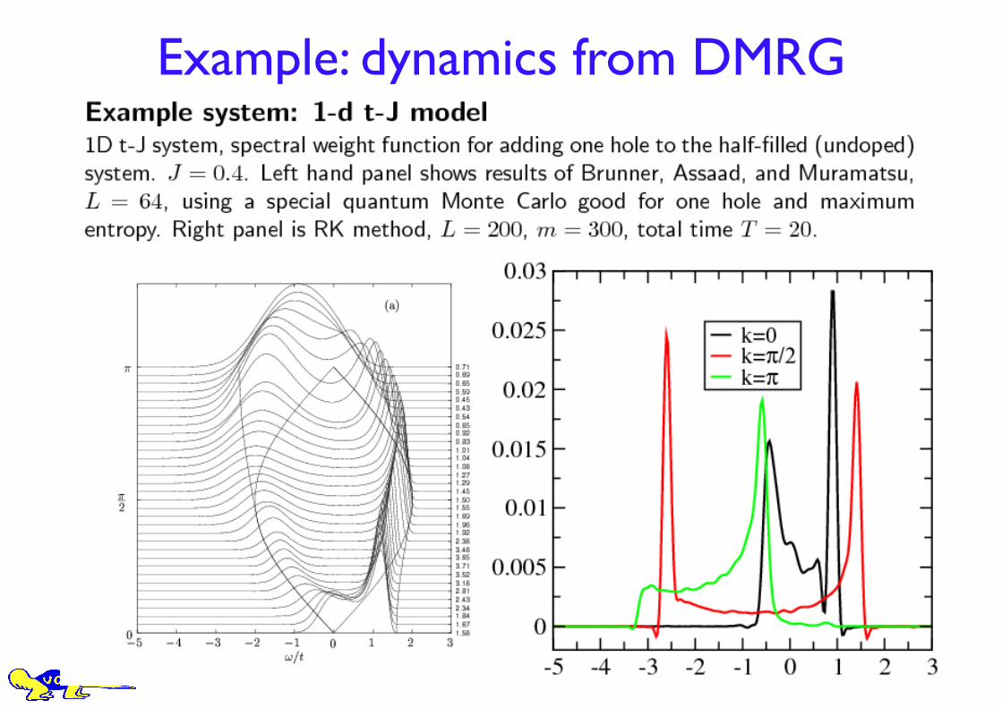
Example: dynamics from DMRG

Example: dynamics for 1D systems

0 1 2!

0

0.1

0.2

0.3

0.4N(!)

Jz=0.125Jz=0.25Jz=0.375Jz=0.5

S=1/2 Chain, XXZ model

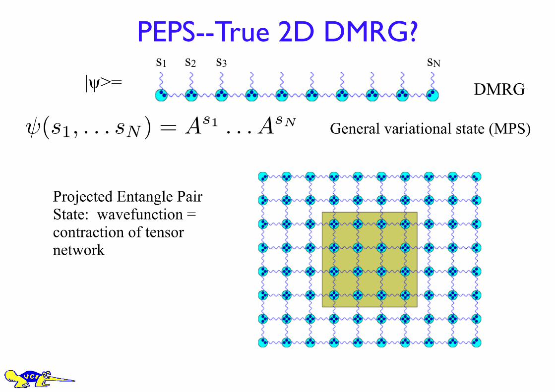
PEPS--True 2D DMRG?s2s1 s3 sN

|ψ>=

!(s1, . . . sN ) = As1 . . . AsN

DMRG

Projected Entangle Pair State: wavefunction = contraction of tensor network

General variational state (MPS)

PEPS: prospects• Currently, PEPS is less efficient than old-style DMRG

for accessible sizes (e.g. 8x8)• But: calculation time is not exponential (m10)• In the last few months, there have been three papers

combining PEPS with Monte Carlo (m5)

Conclusions

• Algorithmic development has been the key driving force in computation for solid state physics (and other fields!)

• Quantum Information has a lot to teach us about simulations!

• Issues/Discussion:– Why are there so few DMRG/QMC/etc people in the US?– Software

• Languages: fast production versus efficiency; freedom from bugs; large codes versus small codes; time to learn the language

• Software libraries so you don’t have to reinvent the wheel.

advanced computation for complex...

Documents