advanced control techniques for motion control problem
TRANSCRIPT

ADVANCED CONTROL TECHNIQUES FOR
MOTION CONTROL PROBLEM
SHAHID PARVEZ
Bachelor of Engineering in Electronics and Communications
Osmania University, India
June, 1995
Master of Science in Systems Engineering
King Fahd University of Petroleum and Minerals
SaudiArabia
June, 1998
submitted in partial fulfillment of the requirements for the degree
DOCTOR OF ENGINEERING
at the
CLEVELAND STATE UNIVERSITY
December, 2003

This thesis has been approved for the
Department of ELECTRICAL AND COMPUTER ENGINEERING
and the College of Graduate Studies by
Thesis Committee Chairperson, Dr. Zhiqiang Gao
Department/Date
Dr. Dan Simon
Department/Date
Dr. Ana Stankovich
Department/Date
Dr. Sridhar Ungarala
Department/Date
Dr. Sally Shao
Department/Date

To my Mother, Wife and Daughter

ACKNOWLEDGMENT
I would like to express my sincere most appreciation and thanks to Dr. Zhiqiang
Gao, my principal advisor, for his continuous support, direction, help and encourage-
ment. He was available for guidance at all times. I learned a lot from his problem
solving methodology and new ideas.
Thanks to my committee members Dr. Simon, Dr. Stankovic, Dr. Ungarala
and Dr. Shao, for their support and help during the dissertation.
I would also like to thank my mother, wife, daughter and all my family mem-
bers for all their continuous moral support, encouragement, inspiration and immense
sacrifices. Finally, I would like to thank all my friends and colleagues at CACT for
their help and making this period a memorable one.
iv

ADVANCED CONTROL TECHNIQUES FOR
MOTION CONTROL PROBLEM
SHAHID PARVEZ
ABSTRACT
Common methods used for solving low-frequency mechanical resonance in in-
dustrial servo systems are often inadequate. Linear and non-linear algorithms to
cure low frequency mechanical resonance are proposed. A novel controller based on
the multi-resolution decomposition property of wavelets, called the Multiresolution
Wavelet Controller is developed. The controller is similar to a Proportional-Integral-
Derivative controller in principle and application. The output from a motion con-
trol system represents the cumulative effect of uncertainties such as measurement
noise, frictional variation and external torque disturbances, which manifest at differ-
ent scales. The wavelet is used to decompose the error signal into signals at different
scales. These signals are then used to compensate for the uncertainties in the plant.
This controller is further applied to other industrial applications to validate the con-
trol scheme. A scheme to generate low noise differential signal using wavelets is also
developed. Wavelet transforms are investigated for their ability to solve industrial
control issues such as noise, disturbance, and improving loop bandwidth.
v

TABLE OF CONTENTS
Page
ACKNOWLEDGMENT . . . . . . . . . . . . . . . . . . . . . . . . . . . . . . iv
ABSTRACT . . . . . . . . . . . . . . . . . . . . . . . . . . . . . . . . . . . . v
LIST OF TABLES . . . . . . . . . . . . . . . . . . . . . . . . . . . . . . . . . ix
LIST OF FIGURES . . . . . . . . . . . . . . . . . . . . . . . . . . . . . . . . x
CHAPTER
I. INTRODUCTION . . . . . . . . . . . . . . . . . . . . . . . . . . . . . . . 1
II. BACKGROUND AND LITERATURE REVIEW . . . . . . . . . . . . . 5
2.1 Low-Frequency Resonance Model . . . . . . . . . . . . . . . . . . 7
2.2 Review of Existing Techniques . . . . . . . . . . . . . . . . . . . 13
2.2.1 Low-pass and notch filters . . . . . . . . . . . . . . . . . 14
2.2.2 Acceleration Feedback . . . . . . . . . . . . . . . . . . . . 16
2.3 Motivation . . . . . . . . . . . . . . . . . . . . . . . . . . . . . . 17
III. WAVELETS AND MULTIRESOLUTION ANALYSIS . . . . . . . . . . 19
3.1 From Fourier to Wavelets . . . . . . . . . . . . . . . . . . . . . . 20
3.1.1 Essence of Wavelet . . . . . . . . . . . . . . . . . . . . . . 23
3.2 Multiresolution Analysis . . . . . . . . . . . . . . . . . . . . . . . 24
3.2.1 Scaling and Wavelet Functions and Filters . . . . . . . . . 27
3.3 Signal Decomposition Process . . . . . . . . . . . . . . . . . . . . 29
vi

3.3.1 Multiresolution Wavelet Controller . . . . . . . . . . . . . 31
3.4 Implementation Issues . . . . . . . . . . . . . . . . . . . . . . . . 37
3.4.1 Signal Pipeline Architecture . . . . . . . . . . . . . . . . 37
3.4.2 Number of Decomposition Levels . . . . . . . . . . . . . . 38
3.4.3 Selection of Wavelet . . . . . . . . . . . . . . . . . . . . . 39
3.4.4 Error Signal Analysis . . . . . . . . . . . . . . . . . . . . 40
3.4.5 Best Basis Selection . . . . . . . . . . . . . . . . . . . . . 40
3.5 Tuning the Gains of the Controller . . . . . . . . . . . . . . . . . 42
3.5.1 Observations and framework of a Multiresolution Wavelet
Controller . . . . . . . . . . . . . . . . . . . . . . . . . . 43
3.6 Generalized Multiresolution Controller . . . . . . . . . . . . . . . 45
IV. APPLICATIONS OF MULTIRESOLUTION WAVELET CONTROLLER 47
4.1 Temperature Regulation Problem . . . . . . . . . . . . . . . . . . 47
4.2 Position Control System . . . . . . . . . . . . . . . . . . . . . . . 49
4.2.1 Experimental Results . . . . . . . . . . . . . . . . . . . . 51
4.3 Wavelet Differentiator . . . . . . . . . . . . . . . . . . . . . . . . 54
4.3.1 Differentiation Procedure . . . . . . . . . . . . . . . . . . 55
4.3.2 Comparison of Differentiators . . . . . . . . . . . . . . . . 56
4.4 Improving the PID performance using wavelets . . . . . . . . . . 58
4.4.1 PID using wavelet differentiator . . . . . . . . . . . . . . 58
4.4.2 PID using denoised error . . . . . . . . . . . . . . . . . . 59
4.4.3 PID using denoised error and wavelet differentiator . . . . 59
V. TECHNIQUES FOR LOW-FREQUENCY RESONANCE CONTROL . 62
vii

5.1 Baseline System . . . . . . . . . . . . . . . . . . . . . . . . . . . 64
5.2 Profile Modification . . . . . . . . . . . . . . . . . . . . . . . . . 66
5.3 Nonlinear PI Control . . . . . . . . . . . . . . . . . . . . . . . . 68
5.4 Acceleration Feed-forward with Nonlinear Servo gains . . . . . . 71
5.5 Discrete Time Optimal Control . . . . . . . . . . . . . . . . . . . 73
5.6 Active Disturbance Rejection Control . . . . . . . . . . . . . . . 75
5.6.1 Extended State Observer . . . . . . . . . . . . . . . . . . 76
5.7 Single Parameter Tuning . . . . . . . . . . . . . . . . . . . . . . 79
5.7.1 Linear Extended State Observer . . . . . . . . . . . . . . 80
5.7.2 Parameterization of Linear Extended State Observer . . . 81
5.7.3 Controller Parameterization . . . . . . . . . . . . . . . . . 83
5.7.4 Linear Active Disturbance Rejection Control . . . . . . . 84
5.8 Multiresolution Wavelet Controller . . . . . . . . . . . . . . . . . 86
5.9 Summary of Results . . . . . . . . . . . . . . . . . . . . . . . . . 89
VI. CONCLUSIONS AND FUTURE WORK . . . . . . . . . . . . . . . . . 93
6.1 Future Work . . . . . . . . . . . . . . . . . . . . . . . . . . . . . 94
BIBLIOGRAPHY . . . . . . . . . . . . . . . . . . . . . . . . . . . . . . . . . 96
APPENDIX . . . . . . . . . . . . . . . . . . . . . . . . . . . . . . . . . . . . . 99
A. Wavelet Multiresolution Controller Code . . . . . . . . . . . . . . . 99
B. Wavelet Filter Coefficeints . . . . . . . . . . . . . . . . . . . . . . . 118
INDEX . . . . . . . . . . . . . . . . . . . . . . . . . . . . . . . . . . . . . . . 120
viii
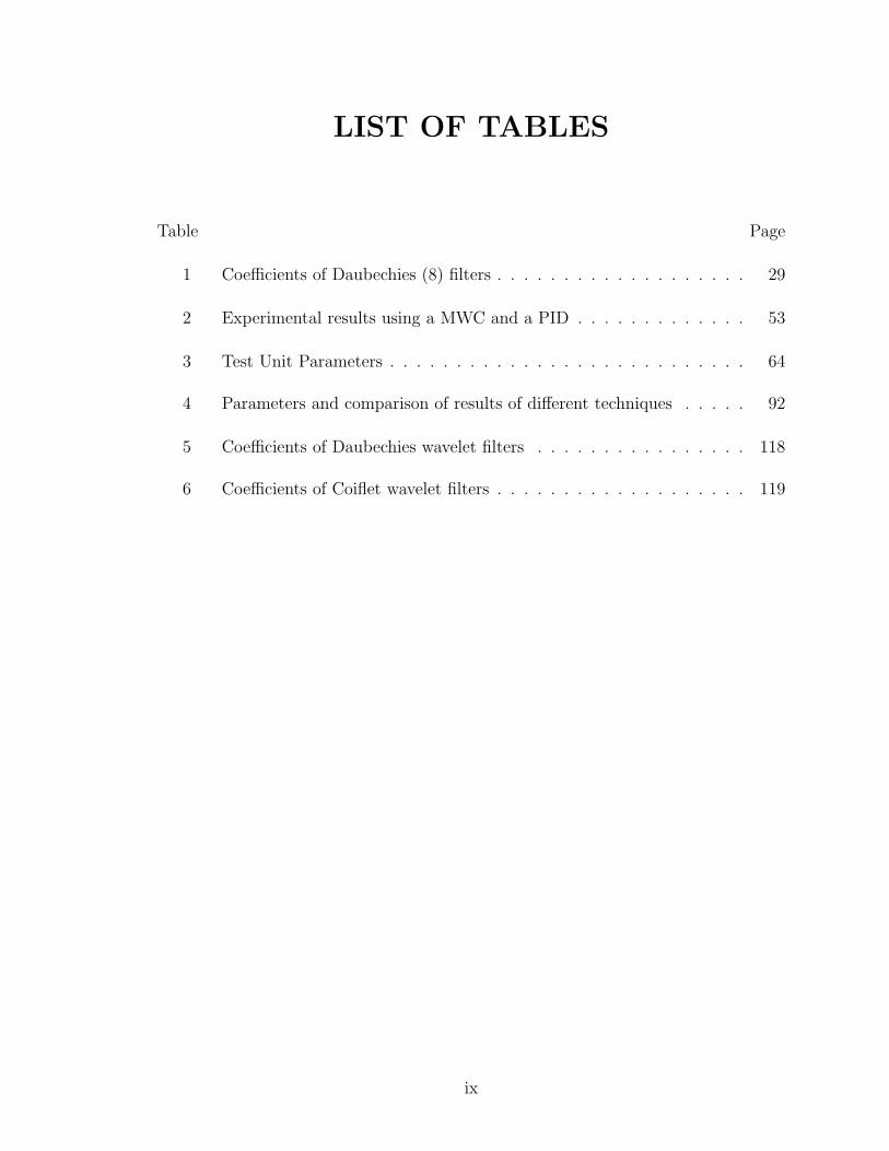
LIST OF TABLES
Table Page
1 Coefficients of Daubechies (8) filters . . . . . . . . . . . . . . . . . . . 29
2 Experimental results using a MWC and a PID . . . . . . . . . . . . . 53
3 Test Unit Parameters . . . . . . . . . . . . . . . . . . . . . . . . . . . 64
4 Parameters and comparison of results of different techniques . . . . . 92
5 Coefficients of Daubechies wavelet filters . . . . . . . . . . . . . . . . 118
6 Coefficients of Coiflet wavelet filters . . . . . . . . . . . . . . . . . . . 119
ix

LIST OF FIGURES
Figure Page
1 Simple compliantly-coupled motor and load . . . . . . . . . . . . . . 7
2 Block diagram of a compliantly-coupled load . . . . . . . . . . . . . . 8
3 Plot of motor/load plant gain vs. frequency . . . . . . . . . . . . . . 9
4 Velocity control system . . . . . . . . . . . . . . . . . . . . . . . . . . 9
5 Open loop Bode plot of rigid and compliant plant . . . . . . . . . . . 10
6 Effect of low frequency resonance in time response of the plant . . . . 11
7 Open loop gain of compliant system with and without low-pass filter 15
8 Acceleration feedback . . . . . . . . . . . . . . . . . . . . . . . . . . . 17
9 Wavelet Functions . . . . . . . . . . . . . . . . . . . . . . . . . . . . 28
10 Decomposition Analysis . . . . . . . . . . . . . . . . . . . . . . . . . 31
11 Decomposition Synthesis . . . . . . . . . . . . . . . . . . . . . . . . . 31
12 Block diagram of a plant using a PID . . . . . . . . . . . . . . . . . . 33
13 Block diagram of a plant using a Multiresolution Wavelet Controller . 34
14 Comparison of PID and multiresolution decomposed signals . . . . . 36
15 Signal pipeline architecure . . . . . . . . . . . . . . . . . . . . . . . . 38
16 Dictionary of Error Signals . . . . . . . . . . . . . . . . . . . . . . . . 41
17 Block diagram of a plant using a Generalized Multiresolution Controller 46
18 Block diagram of a temperature regulation problem . . . . . . . . . . 49
x

19 Simulation response of a temperature regulation plant under different
time delays . . . . . . . . . . . . . . . . . . . . . . . . . . . . . . . . 50
20 Block diagram of a DC brush-less servo system . . . . . . . . . . . . 51
21 MWC and PID responses to torque disturbance . . . . . . . . . . . . 53
22 Block diagram of differentiators . . . . . . . . . . . . . . . . . . . . . 56
23 Comparison of differentiators . . . . . . . . . . . . . . . . . . . . . . 57
24 Block diagram of a plant using a PID controller with wavelet differen-
tiated error . . . . . . . . . . . . . . . . . . . . . . . . . . . . . . . . 58
25 Block diagram of a plant using a wavelet denoised error signal . . . . 59
26 Block diagram of a plant using a denoised error and wavelet differen-
tiated error signal . . . . . . . . . . . . . . . . . . . . . . . . . . . . . 60
27 Simulation results on a plant using wavelets in different PID configu-
rations . . . . . . . . . . . . . . . . . . . . . . . . . . . . . . . . . . . 60
28 Test-unit mechanism . . . . . . . . . . . . . . . . . . . . . . . . . . . 64
29 Implementation block diagram of motor . . . . . . . . . . . . . . . . 65
30 Step response of the baseline system . . . . . . . . . . . . . . . . . . 65
31 A profile generator . . . . . . . . . . . . . . . . . . . . . . . . . . . . 66
32 Response of the system using a profile . . . . . . . . . . . . . . . . . 67
33 Plot of nonlinear function vs. error . . . . . . . . . . . . . . . . . . . 69
34 Block diagram of the plant using an NPI Controller . . . . . . . . . . 69
35 Command response using a NPI controller . . . . . . . . . . . . . . . 70
xi

36 Block diagram of motor with Acceleration Feed-forward and Nonlinear
gains . . . . . . . . . . . . . . . . . . . . . . . . . . . . . . . . . . . 71
37 Command response using Acceleration Feed-forward and NPI . . . . 72
38 DTOC based implementation of the plant . . . . . . . . . . . . . . . 74
39 Command response using a DTOC . . . . . . . . . . . . . . . . . . . 75
40 Block diagram for ADRC structure . . . . . . . . . . . . . . . . . . . 78
41 Simulation result using ADRC . . . . . . . . . . . . . . . . . . . . . 78
42 Observed velocity using LESO . . . . . . . . . . . . . . . . . . . . . . 82
43 Simulation block diagram using LADRC . . . . . . . . . . . . . . . . 85
44 Response of the plant using Single Parameter Tuning . . . . . . . . . 85
45 Simulation response using a Multiresolution Wavelet Controller . . . 87
46 Effect of noise during steady state response . . . . . . . . . . . . . . . 88
47 Comparison of results . . . . . . . . . . . . . . . . . . . . . . . . . . . 90
xii
CHAPTER I
INTRODUCTION
Servo system inertia mismatch, between load and motor, has long been a con-
cern for the motion system designer. Most problems of resonance are caused by
compliance created by transmission components and the inertia mismatch between
motor and load. The resonance problem has seen a recent surge on account of two
sources: the need for ever increasing levels of servo performance and the use of syn-
chronous permanent magnets which reduced the size (inertia) of the motor. These
motors allow more torque to be produced with smaller motors. This usually increases
the inertia mismatch, which exacerbates the problem of low frequency resonance.
For a servo system to operate effectively, servo amplifiers need to be tuned to
optimize the response of the system, which includes command response and distur-
bance rejection. Standard servo control laws are structured for rigidly-coupled loads.
However, in practical machines some compliance is always present; this compliance
1

2
in addition to the inertia mismatch reduces control-loop stability margins, forcing
servo gains down, which reduces machine performance. Stiffening the components
can increase the machined cost significantly. Stiffer components not only cost more,
they require tighter mechanical tolerance in the machine structure.
Mechanical resonance falls into two broad categories: low-frequency and high-
frequency. High-frequency resonance causes control-system instability at the natural
frequency of the mechanical system, typically between 500Hz and 1200 Hz. Low-
frequency resonance causes instability well below the natural frequency of the me-
chanical system, at a frequency that coincides with the first phase crossover of the
servo loop (the frequency where the open loop phase first falls to −180o), typically
between 100 to 400Hz. Low-frequency resonance occurs much more often in general
industrial machines. The distinction between these resonance types is rarely made
in the literature, although it is crucial to be aware of it when finding a remedy to
resonance problems.
The problem of load resonance is well studied and numerous active and passive
solutions have been developed. However, the literature on active cures deals almost
entirely with the less common, high-frequency resonance. Active solutions that are
effective for high-frequency resonance, such as low-pass filters, often do not help and
even can exacerbate problems with low-frequency resonance.
It is broadly accepted that physical phenomenon occur at different time scales.
However, it is not clear how to incorporate this knowledge systematically into provid-
ing basic process problems such as control, resonance, noise, disturbance etc. There is
a need to provide explicit representation of the control action with localization in both

3
time and frequency. This is where the wavelet theory comes into play. The wavelet
theory, developed earlier as a mathematical tool, has in recent years been used in
various industrial applications. Wavelets are known for their extensive applications
in the field of signal processing. They are effective in estimating trends, breakdown
points and discontinuities in higher derivatives. Wavelets possess two properties that
make them especially valuable for data analysis: they reveal local properties of the
data and they allow multi-scale analysis. Their locality is useful for applications
that require online response to changes, such as controlling a process. Recently some
work has been reported on use of time-frequency localization of wavelet transforms
in process control industry [3, 4, 22]. Based on the multiresolution decomposition
property of wavelets, a Multiresolution Wavelet Controller(MWC) analogous to a
Proportional-Integral-Derivative(PID) controller is proposed.
A PID controller is widely used across the industry. It is easy to implement and
relatively simple to tune. In general, a PID controller takes as its input the error(e),
acts on the error to generate a control output(u). Similarly a MWC decomposes
the error signal into its high, low and intermediate frequency components, using the
multiresolution decomposition property of the wavelets. Each of these components
are scaled by their respective gains, and then added together to generate the control
signal u. The output from a system represents the cumulative effect of many under-
lying phenomena such as process dynamics, measurement noise, effects of external
disturbances etc., which manifest on different scales. The wavelet decomposition,
which represents the error signal at different scales, enables us to compensate for
these uncertainties dynamically in the controller. Based on the results obtained using

4
wavelet transforms on the motion control problem, this scheme is further investigated
for its applicability on other industrial problems.
In industry the primary issue with differentiation has been noise corruption. It
is known that a pure differentiation is not physically realizable due to its noise ampli-
fication property. Finding an approximate differentiation with good noise immunity
is paramount in achieving high control performance. A novel signal processing scheme
using Daubechies wavelets is used to generate an almost noise free differential signal.
This scheme can be greatly utilized to improve performance of control systems in
different fields.
Background of the low frequency mechanical resonance problem, review of ex-
isting techniques and literature review are given in chapter 2. Background of wavelets,
computational aspects of wavelet transforms and selection of wavelets are detailed
in chapter 3. Application of the wavelet controller in other fields of controls and
wavelet based differentiation scheme are discussed in chapter 4. Several new concepts
and methods, such as the use of nonlinear servo gains, profile modification, param-
eterization and multiresolution analysis are discussed and applied for low frequency
mechanical resonance reduction in chapter 5. Conclusions and future work on the
related field are given in chapter 6.

CHAPTER II
BACKGROUND AND LITERATURE
REVIEW
It is well known that servo performance, such as command response and dis-
turbance rejection, is enhanced when control-law gains are high. Newtonian physics
teaches that F (force) = M(mass)∗A(acceleration), or in rotary terms, T (torque) =
J(inertia) ∗ A(acceleration). This fundamental equation shows that the lesser iner-
tia a system has, the lesser torque it will take to meet a desired acceleration rate.
For this reason it is advantageous to minimize inertia to the greatest possible extent
in order to maximize acceleration. For a fixed amount of load inertia this means
minimizing motor inertia. Stated another way, minimizing motor inertia would allow
most of the motor’s torque being used to accelerate the load, not wasting much of the
motor’s torque accelerating its own inertia. In conclusion, minimizing motor inertia
for a given rating of torque will theoretically maximize acceleration, increase system
5

6
bandwidth, but at the same time, increase load to motor inertia mismatch.
For a servo system to operate effectively, servo amplifiers need to be tuned
to optimize the response of the system. Improving the response of the system often
involves increasing controller gains. Control-loop instability results when a high-gain
control law is applied to a compliantly-coupled motor and load and at times it also
leads to uncontrollable oscillations. The goal is to tune the system for maximum
responsiveness with the minimum of instability. Instability begins with overshoot
with respect to the speed for which the motor has been given a command. A good
compromise between responsiveness and stability is for the system to have critical
damping and phase shift not exceeding 900. Slightly higher phase shift has been
suggested possible, based on variations in system requirements, mechanics and con-
troller. Critical damping defines an overshoot of less than 5 %. The particular gains
to achieve this response are based on factors such as system inertia and friction, to
mention just two. Inertia is a key variable that may change in a system as a result
of various factors. If inertia changes to too great an extent, the amplifier tuning may
become unacceptable.
Machine designers normally specify transmission components, such as cou-
plings and gearboxes, to be rigid in an effort to minimize mechanical compliance.
However, some compliance in transmission components is unavoidable. In addition,
marketplace limitations, such as machine cost, size, and weight, frequently force de-
signers to choose lighter-weight components than would otherwise be desirable. Often,
the resulting rigidity of the transmission is so low that instability results when control-
law gains are raised to levels needed to achieve the desired servo performance. The

7
well-known lumped-parameter model [3] for a compliant coupling is shown in Figure
1. The motor with inertia JM produces a torque TM which is used to drive a load of
inertia JL. The equivalent spring constant of the entire transmission is represented
by KS.
Figure 1: Simple compliantly-coupled motor and load
2.1 Low-Frequency Resonance Model
A schematic diagram of the compliantly coupled mechanism of Figure 1 is
shown in Figure 2. Here, the equivalent spring constant of the entire transmission is
KS; also, to represent loss-producing properties, a mechanical damping term is shown
producing torque proportional to the velocity difference via cross-coupled viscous
damping, bS. Note that this model assumes the inertia of each of the transmission
components is small and that the load can be characterized as a single, rigid inertia.
This model does not include Coulomb friction or stiction as these effects are secondary
in the study of resonant behavior.
The transfer function from electromechanical torque TE, to motor velocity, VM ,
is
VM
TE
=1
JM + JL
1
s
JLs2 + bSs+KS
JLJM
JL+JMs2 + bSs+KS
(2.1)

8
Figure 2: Block diagram of a compliantly-coupled load
which is a single, lumped inertia, 1/[(JM + JL)], modified by a bi-linear quadratic or
bi-quad function. Eq. 2.1 represents the plant in the case where the position feedback
sensor is on the motor (as opposed to the load), as is common in industry. The ideal
plant for traditional control laws, such as PI and PID, is a scaled integrator. As
shown in Eq. 2.1, the bi-quad term corrupts the integrator. The bi-quad term has
its minimum gain at FAR and its maximum gain at FR as shown in Eq. 2.2 and in
Figure 3, which is a Bode plot of Eq. 2.1.
FAR = 12π
√KS
JL
FR = 12π
√KS
JLJMJL+JM
(2.2)
The effect of the bi-quad term can be seen in Figure 3. Where the load rigidly
coupled to the motor, the model would be a single inertia equal to the sum of the
motor and load inertias. This transfer function is shown as the lower dashed line in
Figure 3. However, the bi-quad corrupts the plant at and above the anti-resonant
frequency, FAR. The effect seen in the gain is attenuation at and around FAR and
amplification at, around, and above FR.
The key problem presented by a compliant coupling for low-frequency reso-

9
Figure 3: Plot of motor/load plant gain vs. frequency
nance [2] is the net increase in gain above the resonant frequency, FR. As shown
in Figure 3, below FR, the plant behaves like a simple integrator, KT/[s(JM + JL)].
Also, above FR, the transfer function behaves like a simple integrator. However, the
gain of the plant is substantially increased compared to the gain well below FAR.
Above FR, the load is effectively disconnected from the motor so that the gain of the
plant is a function of inertia of the motor only, KT/[sJM ]. Figure 4 shows a velocity
control system. The velocity error(VE), formed by the difference of the command(VC)
and feedback(VF ), is processed by a control law and an optional set of filters. The
torque command, TC , is connected to the current controller, which produces TE, elec-
tromagnetic torque, via current in the motor. The motor/load plant is connected
to an encoder/resolver. The tendency towards instability caused by the corrupting
Figure 4: Velocity control system

10
Figure 5: Open loop Bode plot of rigid and compliant plant
bi-quad term in Eq. 2.2 is most easily seen in the open-loop Bode plot of the ve-
locity controller of Figure 5. The open-loop transfer function describes the effect of
traversing the loop from VE to VF . The open-loop Bode plot is well-known to predict
stability problems using two measures: phase margin(PM) and gain margin(GM) [2].
This is based on the principle that if there is unity gain (0 dB) and −1800 phase
lag at the same frequency, complete instability will result. For a stable system, PM
is the difference of −1800and the phase of the open loop at the gain crossover, the
frequency where the gain of the open loop is 0 dB. GM is the negative of the gain of
the open loop at the phase crossover, the frequency where the open-loop phase crosses
through −1800. The open-loop plots for a rigidly-coupled and a compliantly-coupled
load demonstrate the cause of low-frequency resonance as shown in Figure 5. The
harmful effects of the compliantly coupled load are most easily seen in the gain mar-
gin. As marked in Figure 5, when the resonant frequency is well below the first phase

11
crossover, the effect of the compliant load is to reduce the GM; the amount of reduc-
tion will be approximately (JM + JL)/JM (the distance between the two dashed lines
in Figure 5). If JL/JM (the so-called inertia mismatch) is 5, the reduction of GM will
be 6 or a factor of about 15 dB. Assuming no other remedy were available, the gain of
the compliantly-coupled system would have to be reduced by 15 dB, compared to the
rigidly-coupled system, assuming both systems would have to maintain the same GM.
Such a large reduction in gain would translate to a system with a greatly reduced
command response and a similarly reduced disturbance rejection. Figure 6 shows the
Figure 6: Effect of low frequency resonance in time response of the plant
effect of increasing gains of a compliantly-coupled plant. Gains have to be increased
to improve plant robustness, disturbance rejection and reduce the transient time of

12
the plant. However, by doing so, the plant is driven close to instability as can be
seen from Figure 6(a) and (b). The only alternative under the present circumstance
is to cut down on the gains to improve the margin of stability or to use a resonance
reduction technique which is the focus of this research.
It should be pointed out that an alternative form of resonance, high-frequency
resonance [2], occurs under different conditions. High-frequency resonance is the con-
dition where the natural frequency of the mechanical system(FR), is well above the
first phase crossover. In this case, the plant is lightly damped and the gain near
FR forms a strong peak reaching well above the gain of KT/[JMs], the approximate
maximum of the system shown in Figure 5. With high-frequency resonance, this
peak reaches well up, usually at the 2nd or 3rd phase crossover, where the base gain
is typically less than -30dB. However, the gain caused by a lightly damped bi-quad
term in Eq. 2.1 can be greater than 60dB. While both types of resonance are caused
by compliance, the relationship of the FR and the first phase crossover changes the
remedy substantially; infact, reliable cures of high-frequency resonance, especially
low-pass filters, exacerbate problems with low-frequency resonance. The mechanical
structures that cause high-frequency resonance, especially stiff transmission compo-
nents and low mechanical damping, are typical of high-end servo machines such as
machine tools. However, the smaller and often more cost sensitive general-purpose
servo machines used in industries such as packaging, assembly, textiles, plotting, and
medical, typically have less rigid transmissions and higher mechanical damping so
that low-frequency resonance is more common in those industries.

13
2.2 Review of Existing Techniques
Low-frequency resonance has become a prevalent problem in industry over the
last 15 years. This change has resulted from two sources: the need for ever increasing
levels of servo performance and the use of synchronous permanent magnet or ”brush-
less DC” motors based on rare-earth magnets. These motors allow more torque to be
produced with a smaller motor. This usually increases the inertia mismatch, which
exacerbates the problem of low-frequency resonance as demonstrated in Figure 5.
The two most common cures for low-frequency resonance are passive: stiffening the
transmission and increasing the motor inertia. Stiffening the transmission can be
an effective cure for low-frequency resonance. This method increases the mechani-
cal stiffness, KS, raising the resonant and anti-resonant frequency, according to Eq.
2.2. If the FR can be increased to a frequency well beyond the first phase crossover,
resonance problems are greatly reduced. However, stiffening the transmission can
significantly increase machine cost. Stiffer components cost more and require tighter
mechanical tolerances in the machine structure. Also, stiffer transmission components
can reduce key performance measures such as when a lead screw is used to replace
a belt-driven mechanism; of these two alternatives to convert rotary motion to lin-
ear, the stiffer lead screw cannot match the acceleration rates of the more compliant
belt drive. Another common passive cure is to increase the motor inertia. Assuming
the load inertia, JL, is fixed, increasing the motor inertia, JM , reduces the inertia
mismatch JL/JM . This solution is so common, that at least one servo manufacturer,
Kollmorgen, provides an option for its highest-accelerating motors where a customer

14
can specify that an inertial flywheel be added to the motor. Unfortunately, increasing
motor inertia has several negative effects. First, it reduces the maximum accelera-
tion of the system. This effect can be mitigated by using a larger motor and drive,
although this increases the cost and size of the machine. Second, it increases the
losses associated with regular cycling of speed such as is common in the manufacture
of discrete parts. This problem is difficult to cure with a larger motor, as larger
motors typically have larger rotors, which further increase the losses associated with
acceleration and deceleration.
2.2.1 Low-pass and notch filters
Two passive methods are commonly provided in general servo drives used in
industry: low-pass filters [2, 3] and notch filters [11, 15]. Neither method works well
for low-frequency resonance. Low-pass filters, such as the two-pole filter in Eq. 2.3,
are effective only when the filter’s bandwidth is set well below FR. In the case of
low-frequency resonance, such a bandwidth is usually far too low to allow reasonable
servo performance. The phase lag generated by the filter is so large that servo gains
have to be reduced greatly to maintain loop stability; the end result is that servo
performance is reduced dramatically below what it could be.
TLP (s) =ωn
2
s2 + 2ζωn + ωn2
(2.3)
The problem with using a low-pass filter on low-frequency resonance is that low-
pass filters generate significant phase lag before they provide attenuation. Returning
to Figure 3, if a low-pass filter with a bandwidth above FR is used, it will introduce

15
phase lag that will reduce the PM, without significantly attenuating the gain near
the first phase crossover; the net effect is that the PM is reduced and the system
becomes less stable. As long as the open-loop gain near FR remains above 0dB, low-
pass filters destabilize the system. Given that the gain of the open loop near FR in
Figure 5 is about 10 dB, the bandwidth of a low-pass filter that could attenuate that
gain to well below 0 dB (say, -10 dB) would have to have a bandwidth well below FR;
unfortunately, the resulting filter severely reduces servo performance because of the
additional phase lag in the control loop. As discussed in [3] the example in Figure
7 required a low-pass filter with a bandwidth of 80 Hz, severely limiting the control
loop, which had a bandwidth of about 25 Hz before the filter was added. After the
filter was added, the stability margins were so small that the servo gains had to be
reduced significantly to avoid excessive overshoot.
Figure 7: Open loop gain of compliant system with and without low-pass filter
Notch filters, such as the two-pole notch in Eq. 2.4, are generally ineffective on
low-frequency resonance. The function of a notch filter in high-frequency resonance
[11] is to attenuate the relatively narrow gain peak induced by the lightly damped

16
mechanisms that are subject to that problem. However, with low-frequency reso-
nance, the gain peak is much broader; for example, in Figure 7, the frequency range
where the compliant-system open-loop gain exceeds 0 dB is about 150 Hz to 400 Hz,
far too broad for a notch. Thus, notch filters often do not improve performance of
systems with low-frequency resonance.
TNOTCH(s) =s2 + ωn
2
s2 + 2ζωn + ωn2
(2.4)
2.2.2 Acceleration Feedback
Acceleration feedback (using both directly measured and observed accelera-
tion) has been documented in several papers [3, 6, 9, 12, 13, 20]. Ideal acceleration
feedback has the same effect on stability as increasing JM , but it does so without the
drawbacks of increased motor inertia such as increased size and weight, or the re-
quirement of a larger drive to maintain acceleration rates [3, 12]. In practice, directly
measured acceleration feedback is noisy, especially in the case where acceleration is
formed by taking the second difference of position. Resolution limitations in the
position signal create severe noise spikes on the acceleration signal.
An alternative method of computing acceleration is to use an observer [3] as
shown in Figure 8. Observers are well known for improving the quality of feedback
signals. As discussed in [3], KA was limited to a maximum of about 2.5 before the
observer-based acceleration term induced instability. In [3], acceleration feedback
was shown by experimentation to be the most effective of several linear methods in
reducing resonance. Acceleration feedback allowed a substantial increase in the servo

17
Figure 8: Acceleration feedback
gains and the corresponding bandwidth of the servo loop. Other alternative methods
have been used to remedy resonance [25]. In addition to the low-pass and notch
filters, the use of a bi-quad filter has been suggested [3].
2.3 Motivation
Low frequency mechanical resonance is a pervasive problem in industry. Most
solutions to solve resonance were developed to solve high frequency resonance. These
solutions fall short of providing an effective solution, and often exacerbate the prob-
lem. The goal of this research work is to provide active software solutions to the low
frequency resonance problem. Recently a new design framework based on nonlinear
mechanisms for application to disturbance rejection has been found to be greatly effi-
cient. These schemes include nonlinear differentiator, nonlinear proportional-integral-
derivative(NPID) and active disturbance rejection control(ADRC). These techniques
are investigated for their ability to solve the resonance problem. Although resonance
is a frequency phenomenon, it occurs at a particular time scale. This problem can
be effectively addressed by explicitly representing the control action with localization
in both time and frequency. This is where the wavelet theory comes into play. The

18
wavelet theory, developed earlier as a mathematical tool, has in recent years been
used in various industrial applications. Wavelets possess two properties that make
them especially valuable for data analysis: they reveal local properties of the data
and they allow multi-scale analysis. However, noncausal nature of the wavelets in-
troduces delay in the computation of the wavelet transform. This delay has hindered
the application of wavelets in controls. Because of the high potential offered by the
wavelets and their practical limitations in controls; this research is focused on provid-
ing wavelet based solutions to control system issues such as noise, disturbance, system
bandwidth and generating a denoised differential signal. Based on the multiresolution
decomposition property of wavelet a novel Multiresolution Wavelet Controller(MWC)
analogous to a Proportional-Integral-Derivative(PID) controller is proposed. Based
on the scope and focus of this research work, a detailed discussion of wavelets and its
mathematical aspects are presented in the next chapter.

CHAPTER III
WAVELETS AND MULTIRESOLUTION
ANALYSIS
The mathematical framework necessary for using wavelets is established in this
chapter. First a brief review of Fourier series is given to provide motivation and show
its similarity to wavelet series representation of signals. Fourier series, or expansion
of periodic functions in terms of harmonic sines and cosines, dates back to the early
part of the 19th century when Fourier proposed harmonic trigonometric series. The
first wavelet was found by Haar in the twentieth century. But the construction of
more general wavelets to form bases for square-integrable functions was investigated
in 1980’s along with efficient algorithms to compute the expansion. At the same
time, applications of these techniques in signal processing have blossomed. While
linear expansions of functions are a classic subject, the recent constructions contain
interesting new features. For example, wavelets allow good resolution in time and fre-
19

20
quency. This feature is important for non-stationary signal analysis. While Fourier
basis is given in closed form, many wavelets can only be obtained through a compu-
tational procedure (and even then, only at specific rational points). While this might
seem as a drawback, it turns out that if one is interested in implementing a signal
expansion on real data, then a computational procedure is better than a closed-form
expression.
In Section 3.1, a brief review of Fourier series is given . Section 3.2 gives an
introduction to wavelet transforms. Section 3.3 shows relationship between wavelet
series representation and multiresolution decomposition. The framework of a MWC
and its implementation issues are discussed in Sections 3.4-6.
3.1 From Fourier to Wavelets
Fourier series representation of a periodic signal f(t) with period T , in terms
of sine and cosines as basis functions is given by
f(t) =1
2a0 +
∞∑i=1
(aicos2πkt+ bisin2πkt)
ai =2
T
∫f(t)cos2πkt dt (3.1)
bi =2
T
∫f(t)sin2πkt dt
Besides its obvious limitation to periodic signals, it has very useful properties,
such as convolution, which comes from the fact that basis functions are eigen func-
tions of linear time-invariant systems. The extension of the scheme to nonperiodic
signals, by segmentation and piecewise Fourier series expansion of each segment, suf-

21
fers from artificial boundary effects and poor convergence at boundaries due to Gibbs
phenomenon.
An attempt to create local Fourier bases is the Gabor transform or short-time
Fourier transform(STFT). A smooth window is applied to the signal and a Fourier
expansion is applied to the windowed signal. This leads to a time-frequency represen-
tation since we get an approximate information about the frequency content of the
signal at the center of the windowed signal. While the STFT has proven useful in
signal analysis, there are no good orthonormal bases based on this construction. Also,
a logarithmic frequency scale, or a constant relative bandwidth, is often preferable to
the linear frequency scale obtained with the STFT.
Let us assume that the signal has a combination of frequencies. If a short
window is used, high frequency components can be located (or resolved) very well in
time; however, short duration windows are insufficient for analyzing low frequency
components. Thus one might conclude that longer windows should be used. If a
long window is used, low frequency components can be analyzed: that is, the signal
can be resolved in frequency. Now the high frequency components can no longer be
located very well in time. We sacrificed time resolution for frequency resolution. This
trade-off between localization in time and frequency is referred to as the Heisenberg’s
uncertainty principle. Simply put, just as one cannot know the exact momentum and
location of the electron simultaneously, one cannot know the exact frequency and
location of the signal component simultaneously. However, one can know the time
intervals in which certain bands of frequencies exist. For lower frequencies we can
choose longer time intervals (or windows). We gain knowledge about the frequency of

22
the signal component, but we loose knowledge about the time location of the signal
component. For higher frequencies, we can choose shorter time intervals. We gain
knowledge about the time location of the signal component, but we loose knowledge
about the frequency of the signal component. This varying of the time interval or
window length is exactly what the wavelet transform accomplishes.
A popular alternative to the STFT is the wavelet transform. Using scales and
shifts of a prototype wavelet, a linear expansion of a signal is obtained. Because the
scales used are powers of an elementary scale factor (typically 2), the analysis uses
a constant relative bandwidth (or, the frequency axis is logarithmic). The sampling
of the time-frequency plane is now very different from the rectangular grid used in
STFT. Lower frequencies, where the bandwidth is narrow (that is the basis functions
are stretched in time) are sampled with a large time step, while high frequencies
(which correspond to short basis functions) are sampled more often. Such a wavelet
scheme gives a good orthonormal basis whereas the STFT does not. The local Fourier
transform retains many of the characteristics of the usual Fourier transform with a
localization given by the window function, which is thus constant at all frequencies.
The wavelet, on the other hand, acts as a microscope, focusing on smaller time phe-
nomenons as the scale becomes small. This behavior permits a local characterization
of functions, which STFT does not.

23
3.1.1 Essence of Wavelet
As the name suggests, a wavelet is a small wave which grows and decays in
a limited period. The contrasting notion is a big wave. An example of a big wave
is a sine wave, which keeps on oscillating up and down. A Wavelet Transform is
computed by correlating the scaled wavelets with the input signal. When the two
signals are correlated with each other, we obtain a measure of similarity between the
two signals. Thus, when the wavelet transform is computed at a scale such that the
wavelet is compressed, we obtain a measure of how similar the input signal is to the
high frequency wavelet. Likewise, when the wavelet transform is computed at a scale
such that the wavelet is dilated, we obtain a measure of how similar the input signal
is to the low frequency wavelet. This kind of analysis is also called multiresolution
analysis.
A Continuous Wavelet Transform(CWT) can be defined as an inner product
between the shifted and scaled versions of a single function - the mother wavelet
ψ(t), and the function f(t) itself. The resultant coefficients of the function f(t) are
denoted by CWTf (m,n) where m stands for scale and n for shift. Because of the
high redundancy in CWTf (m,n) it is possible to discretize the transform parameters
and still be able to achieve reconstruction.
Consider the family of functions obtained by shifting and scaling a zero-mean
function ψ(t) ∈ L2(R) (is the Banach space, where, each element are square integrable

24
on R), ∫∞−∞ ψ(t)dt = ψ(0) = 0
ψm,n(t) = 1√(|m|)
ψ( t−nm
)
(3.2)
Then the continuous wavelet transform is given by
f(t) =∫∞−∞
∫∞−∞CWTf (m,n)ψ∗m,n(t)dt
CWTf (m,n) =∫
Rψm,n(t)f(t)dt
(3.3)
ψ∗m,n is the complex conjugate of the wavelet ψm,n and the factor 1/√m is used to
conserve the norm. For small m(m < 1), ψm,n(t) will be short and of high frequency,
while for large m(m > 1), ψm,n(t) will be long and of low frequency. Thus a natural
discretization will use large time steps for large m, and conversely choose fine time
steps for small m. Special choices for ψ(t) and the discretization leads to orthonormal
bases or wavelet series. In a similar manner a Discrete Wavelet Transform(DWT) of
a sampled signal f(x) is given by
f(x) =∑
m,n bm,nψ∗m,n(x)
bm,n =∑
x f(x)ψm,n(x)
where, ψm,n is the is wavelet ψ shifted by m at the nth scale.
3.2 Multiresolution Analysis
Multiresolution analysis is a convenient framework for hierarchical represen-
tation of functions or signals on different scales. The basic idea of multiresolution
analysis is to represent a function as a limit of successive approximations. Each of
these successive approximations is a smoother version of the original function with

25
more and more of the finer details added. A signal is written as a coarse approxi-
mation (typically a lowpass, subsampled version) plus a prediction error which is the
difference between the original signal and a prediction based on the coarse version.
Reconstruction is immediate: simply add back the prediction to the prediction error.
The scheme can be iterated on the coarse version. It has been found that if the low-
pass filter meets certain constraints of orthogonality, then this scheme is identical to
an oversampled discrete-time wavelet series. Otherwise, the successive approximation
approach is still at least conceptually identical to the wavelet decomposition since it
performs a multiresolution analysis of the signal. Consider a sampled signal, f(x),
and generate the following sequence of approximations [2],
fm(x) =∞∑
n=−∞
fm,nφ(2mx− n)m=0,1,2,... (3.4)
Each approximation is expressed as the weighted sum of the shifted versions of the
same function, φ(τ), which is called the scaling function. If the (m + 1)th approxi-
mations is required to be a refinement of the mth approximation, then the function
φ(2mx), should be a linear combination of the basis functions spanning the space of
the (m+ 1)th approximation, i.e.
φ(2mx) =∑
k
h(k)φ(2m+1x− k) (3.5)
If V (m+1) represents the space of all functions spanned by the orthogonal set, {φ(2m+1x−
k); k ∈ Z, the set of integers}, and V (m) the space of the coarser functions spanned
by the orthogonal set, {φ(2mx− p); p ∈ Z} then V (m) ⊂ V (m+1). Let
V (m+1) = V (m) ⊕W (m) (3.6)

26
then, W (m), is the space that contains the information added upon moving from the
coarser, f (m)(x), to the finer, f (m+1)(x), representation of the original signal, f(x).
Mallat [2] shows that there are spaces, W (m) that are spanned by the orthogonal
translates of a single function, ψ(2mx), thus leading to the following equation
fm+1(x) = fm(x) +∞∑
n=−∞
fm,nψ(2mx− n)m=0,1,2,... (3.7)
The function, ψ(2mx), is called a wavelet and is related to the scaling function
φ(2m+1x), through the following relationship
ψ(2mx) =∑
k
g(k)ψ(2m+1x− k) (3.8)
h(k) and g(k) from a conjugate mirror filter pair. Summarizing the discussion, a
mixed form N -level discrete wavelet series representation of the signal f(x) is given
by
f(x) =∑
k aN,kφN,k(x) +∑N
m=1
∑k bm,kψm,k(x)
am,k =∑
x f(x)φm,k(x)
bm,k =∑
x f(x)ψm,k(x)
(3.9)
where φ(x) and ψ(x) are conjugate functions corresponding to φ(x) and ψ(x) respec-
tively. Interestingly, the multiresolution concept, besides being intuitive and useful in
practice, forms the basis of a mathematical framework for wavelets. One can decom-
pose a function into a coarse version plus a residual, and then iterate this to infinity. If
properly done, this can be used to analyze wavelet schemes and derive wavelet basis.
It can be seen from Eq. 3.9 that a wavelet transform decomposes a signal f(x) into
trend(a) and detail coefficients(b). An efficient approach in computing the Discrete

27
Wavelet Transform(DWT) involves using filters h(k) and g(k) which are found to be
h(k) =√
2∑
x φ(x)φ(2x− k)
g(k) =√
2∑
x ψ(x)ψ(2x− k)
g(k) = (−1)kh(−k + 1)
(3.10)
Eqs. 3.9 and 3.10 provide a hierarchical and fast scheme for the computation of the
wavelet coefficients of a given function. They form the core part of this research work
and are extensively used for signal decomposition.
3.2.1 Scaling and Wavelet Functions and Filters
By definition a wavelet ψ(t) is a small wave that integrates to zero and is
square integrable. Mathematically these two properties can be defined as:
∫∞−∞ ψ(t)dt = 0∫∞−∞ ψ2(t)dt = 1
(3.11)
On the other hand the scaling function φ(t) integrates to zero and is orthogonal
to the wavelet function. These two properties can be defined as:
∫∞−∞ φ(t)dt = 1∫∞
−∞ ψ(t)φ(t)dt = 0
(3.12)
The scaling function is often referred to as the father wavelet and the wavelet function
as the mother wavelet or simply wavelet. A few examples of the wavelet functions
and the scaling functions are plotted in Figure 9.
It was shown earlier in this chapter that an orthonormal discrete wavelet trans-
form can be calculated based on any filter satisfying the properties of a wavelet filter,

28
Figure 9: Wavelet Functions

29
namely summation to zero and orthonormality. A table showing the set of coefficients
corresponding to wavelet and scaling filter and their conjugates for a Daubechies (8)
filter are shown in Table 1. Since the filters are conjugate mirror filter of one an-
other, it is possible to construct the remaining filters from the wavelet filter. Further
examples of these filters are given in Appendix B.
Table 1: Coefficients of Daubechies (8) filters
h -0.0106 0.0329 0.0308 -0.1870 -0.0280 0.6309 0.7148 0.2304g -0.2304 0.7148 -0.6309 -0.0280 0.1870 0.0308 -0.0329 -0.0106h 0.2304 0.7148 0.6309 -0.0280 -0.1870 0.0308 0.0329 -0.0106g -0.0106 -0.0329 0.0308 0.1870 -0.0280 -0.6309 0.7148 -0.2304
3.3 Signal Decomposition Process
The first step in decomposition consists of computing the trend and detail
coefficients. Thereafter, the trend coefficients combined with the scaling function
as a basis is used to regenerate the trend signal (left side of the summation in Eq.
3.9) and detail coefficients using the wavelets as a basis are used to regenerate the
detail signal (right side of the summation in Eq. 3.9. The trend signal captures the
high scale (low frequency) information and detail signal captures the low scale (high
frequency) information contained in the signal f(t). Depending upon the number
of decomposition levels the end product of a multiresolution decomposition is a set
of these signals at different scales (frequencies) as shown in Eq. 3.13. Where, fH
is the high scale signal, fL is the low scale signal and fM i are the medium scale
signals and N is the number of decomposition levels. For example, if a 3-level (N=3)
30
decomposition of error signal is done, it results in one trend signal (low frequency)
and three detail signals (high and intermediate frequency). There is redundancy in
the trend signal hence only one obtained at the last level is chosen. The frequency
information of these decomposed signals is approximate since wavelet doesn’t have a
precise frequency like sines and cosines of Fourier analysis.
f(t) = fH(t) + fM1(t) + ...+ fMN−1(t) + fL(t) (3.13)
The process of decomposition into trend and detail signals uses a sub-band cod-
ing scheme that is illustrated in Figures 10 and 11 . The Discrete Wavelet Transform
can be computed using the filters h(k) and g(k) , which form a Quadrature Conjugate
Mirror filter pair with h(k) and g(k), where h(k) and g(k) are given by Eq. 3.10.
Figure 10 illustrates the analysis part of a three level decomposition scheme using
sub-band coding. The result of the analysis step is a set of intermediate coefficients,
which represent the weights of the original signal in terms of the basis functions used,
namely the scaling function and the wavelet function. The original signal is filtered
with the scaling function and the wavelet function and down-sampled by 2 resulting
in the trend and detail coefficients at level one. The trend coefficients thus obtained
are then used as the original signal and filtered with scaling function and the wavelet
to yield the coefficients at level two. This process is repeated depending upon the
number of decomposition levels desired. The synthesis process involves up-sampling
the coefficients obtained during the analysis step by a factor of two and filtering them
with the corresponding reconstruction filters. The reconstruction filters h(k) and g(k)
are the conjugate filters corresponding to scaling and wavelet filters respectively. The

31
Figure 10: Decomposition Analysis
synthesis process for a three level decomposition is shown in Figure 11. The resultant
signals are the trend signal fH , the detail signal fL, and the intermediate resolution
signals f1 and f2.
Figure 11: Decomposition Synthesis
3.3.1 Multiresolution Wavelet Controller
Although a lot of work has been done in numerical analysis, signal and image
compression using wavelets, the field of control theory has remained largely immune

32
to this growing phenomenon. One application using wavelets in controls includes
U.S.Patent No. 5,610,843, which involves control of MIMO system, and provides a
method for implementing a controller in a system having many sensors and actua-
tors. Additionally, the disclosure involves computing two transfer functions P and Q
(transfer function from actuator to sensor, and transfer function matrix from sensor
back to actuator) using wavelet transforms on a multi-scale basis. The controller K
is then implemented using Q-parameterization as K = (I+PQ)−1Q . U.S.Patent No
6,480,750 provides a means to perform auto-tracking by adjusting the controller(PID)
parameters. A wavelet transformation of the control signal and the output signal is
done. The result of the analysis is transformed into a system of differential equations.
The formulation of the system of differential equations serves to establish a mathe-
matical function which characterizes the response of a plant. Based on the response
from the plant it is possible to document changes in the response characteristics of the
controlled system. It is possible in this way for the controlling system to be adapted
to simply prescribed operating state of the controlled system which keeps recurring
during operation of the controlled system. U.S.Patent No 6,497,099 is similar, but has
a specific application to a steam turbine. Multi-scale modeling and model predictive
control using wavelets has been reported by Stephanopoulos [5]. However, industries
still rely largely on using a PID controller to achieve their control objective.
uPID(t) = KP ∗ e(t) +KI ∗∫e(t) +KD ∗
d
dte(t) (3.14)
PID has been a phenomenon in industry due to its intuitiveness and simplicity

33
Figure 12: Block diagram of a plant using a PID
of tuning. In general, a PID controller takes as its input the error, e, then acts on
the error so that a control output, u, is generated as shown in Eq. 3.14. Gains KP ,
KI and KD are the Proportional, Integral and Derivative gains used by the system
to act on the error, integral of the error, and derivative of the error respectively. In
terms of frequency information the proportional and integral terms tend to capture
the low frequency information of the error signal and derivative captures the high
frequency information of the signal. In a similar manner, a Multiresolution Wavelet
Controller(MWC) decomposes the error signal into its high, low and intermediate
scale components using Eq. 3.10. Each of these components are scaled by their
respective gains, and then added together to generate the control signal u as shown
in Eq. 3.15.
uWC(t) = KH ∗ eH(t) +KM1 ∗ eM1(t) + ...+KMN−1∗ eMN−1
(t) +KL ∗ fL(t) (3.15)
More generally, the control signal can also take on the form of
uWC(t) = KH ∗ fH(eH(t)) +KM1 ∗ fM1(eM1(t)) + ...
+KMN−1∗ fMN−1
(eMN−1(t)) +KL ∗ fL(eL(t)) (3.16)
where, f(.) are linear or non-linear functions of the component of the error signal.
Unlike a PID controller, which has three tuning parameters (gains) a MWC can

34
Figure 13: Block diagram of a plant using a Multiresolution Wavelet Controller
have two or more parameters based on the number of decomposition levels of the
error signal. For example, a one-level decomposition yields a low and a high-scale
component. So a controller with a one-level decomposition using linear functions
(f(.)) will have two gains. In a similar manner a two-level decomposition of the error
signal, results in three signal components. Each of these components can be scaled by
a gain and added to generate the control signal. Thereby yielding a controller with
three tuning parameters. It is often desirable to have larger number of decomposition
levels as it tends to capture larger scale based characteristics of the error signal,
thereby providing greater resolution in control signal generation. A schematic diagram
of a plant using MWC is shown in Figure 13. Since there are a number of different
wavelets, choice of a wavelet affects the performance of the controller. In general,
there are two kinds of choices to make: the system of representation (continuous,
discrete) and the properties of the wavelets themselves: for example, the number of

35
degree of regularity. A common theme in choice is trade off. If more resolution in
frequency is desired, less resolution in time is achieved; if more vanishing moments
are required the size of wavelet has to increase. In motion control application it was
found that ”Daubechies” of order 4 was suitable for implementation. Further details
on selection of wavelets are discussed later in this chapter.
All physical systems are subjected to some types of extraneous signals or noise
during operation. Therefore, in the design of a control system, consideration should
be given so that the system is insensitive to noise and disturbance. The effect of
feedback on noise and disturbance greatly depends on where these extraneous signals
occur in the system. But in many situations, feedback can reduce the effect of noise
and disturbance on the system performance. In practice, disturbance and commands
are often low-frequency signals, whereas sensor noises are often high-frequency signals.
This makes it difficult to minimize the effect of these uncertainties simultaneously. It
is under these conditions that MWC performs extremely well. Figure 14 shows the
comparison of signals generated by applying a PID scheme (error, differential of error
and integral of error) to the error signal and a multiresolution decomposition(low
scale, medium scale and high scale) of the error signal. This decomposition, unlike
the filters commonly utilized in classic control theory, do not distort the components
of the error that one finds useful in the control algorithm. The control signal can
therefore be more aggressive, i.e., faster and more accurate, without the presence of
noise and oscillation on the signal, which causes constant jitter, flutter or chatter
of the device being controlled. This constant control action is not only inaccurate,
it usually leads to accelerated wear and early failure of whatever device is being
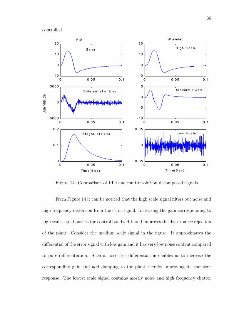
36
controlled.
Figure 14: Comparison of PID and multiresolution decomposed signals
From Figure 14 it can be noticed that the high scale signal filters out noise and
high frequency distortion from the error signal. Increasing the gain corresponding to
high scale signal pushes the control bandwidth and improves the disturbance rejection
of the plant. Consider the medium scale signal in the figure. It approximates the
differential of the error signal with low gain and it has very low noise content compared
to pure differentiation. Such a noise free differentiation enables us to increase the
corresponding gain and add damping to the plant thereby improving its transient
response. The lowest scale signal contains mostly noise and high frequency chatter

37
present in the original signal. By adjusting the lowest scale gain to zero we can
produce a very smooth control signal and drastically reduce the effect of noise on
the plant output. Smooth control effort improves the life of the motor and overall
performance of the plant.
3.4 Implementation Issues
There are a number of practical considerations that must be addressed in order
to come up with a useful wavelet analysis of the time series applicable to controls.
Some of these issues include, the type and size of wavelet to use, how to calculate the
instantaneous wavelet transform of a signal when a sample of signal becomes available
(for real-time control), the number of decomposition levels, the number of samples to
use in the transform.
3.4.1 Signal Pipeline Architecture
Wavelet transform is performed on a bunch of data after it is made available
to the processing engine on account of the non-causal nature of the wavelets. In order
to have causal processing a delay has to be introduced in the channel. This delay is
proportional to the number of samples used in the computation. As control systems
require real-time signal processing in order to operate in real-time, this delay has been
a bottleneck in application of wavelets in controls. Traditionally researchers have
worked with the wavelets on the half axis, which work only on past data or circular
data structure. The other issue that further adds to the delay is the ill-conditioning

38
of the data at the boundaries. In order to perform multi-level decomposition for real
time operation a novel pipeline data architecture is proposed. This architecture is
illustrated in Figure 15. In this scheme a signal buffer of length L is chosen to be
Figure 15: Signal pipeline architecure
2N . Where N is the number of decomposition levels desired in analysis. Initially
the signal buffer is filled with zeros. When the current sample (kth) is available it is
pipelined into the buffer using the First In First Out(FIFO) operation. The signal
buffer values are mirrored and appended so as to have the latest data concentrated
towards the center. The decomposition algorithm is then performed on the resultant
signal buffer. The decomposed kth sample is then available at the center of the signal
buffer.
3.4.2 Number of Decomposition Levels
In order to achieve sufficient resolution in both time and frequency the number
of levels(N) that a signal is decomposed depends upon the size of the signal buffer
(number of observations in the time series) (L) and the size of the filter(F ) used. N
is set to be the largest integer satisfying the equation [1]
N ≤ log2(2 ∗ L− 1
F − 1+ 1) (3.17)

39
From the perspective of a control system, this would represent the number of tuning
parameters in generating the control signal i.e., the gains of the controller. Since the
controller does not have a thresholding scheme, it relies on assigning a zero gain to
the low scale signal for noise immunity. For this reason it was observed that a slightly
larger number of levels than that shown in Eq. 3.17, helped to generate a control
signal with better noise immunity.
3.4.3 Selection of Wavelet
The first problem in constructing a wavelet analysis is the selection of a par-
ticular wavelet from amongst all available ones. A reasonable choice depends upon
the application at hand. In control application the objective is to apply wavelet anal-
ysis on the error signal. The choice that is made here will demonstrate the interplay
between a specific analysis goal (such as signal decomposition to separate noise) and
the properties we need in a wavelet filter to achieve that goal.
It has been found that wavelet of very short widths can sometimes introduce
undesirable artifacts into the resulting analysis that might be desirable in terms
of their small computational effort and real-time applications. On the other hand
wavelet with large number of coefficients can better match the characteristic features
in a time series. Their use can result in more coefficients being unduly influenced
by boundary conditions, some decrease in the degree of localization of DWT coeffi-
cients and an increase in computational burden. An overall strategy is thus to use
the smallest sized filter that gives a reasonable result and also be alignable in time

40
(i.e., phase shift as small as possible).
In the next two sections, the best basis and matching pursuit algorithms are
addressed with the objective of using these algorithms in controls. Best basis is an
optimal orthonormal transformation of the signal. Stephanopoulos proposed a compu-
tational scheme to compute this transformation and called it the best basis algorithm.
This algorithm is used in this research to select a wavelet that can best characterize
an error signal. From the control system perspective, these two algorithms will help
to eliminate the noise from the control signal and enable an increase in the gain cor-
responding to the low frequency signal thereby providing high disturbance rejection
and also bring the steady state error close to zero.
3.4.4 Error Signal Analysis
In order to apply the matching pursuit and best basis algorithms, a dictionary
of error signals was generated. This dictionary comprises of all possible combinations
of error signals that could be generated in a control system environment. Some of
the plots of these signals is shown in Figure 16.
3.4.5 Best Basis Selection
In general a best basis algorithm is used to select a set of basis functions
that can be combined to represent the original signal. Choosing a basis in which to
decompose a signal means selecting certain compromise between time and frequency.
In this research work the selection of wavelets is focused and limited to orthogonal

41
Figure 16: Dictionary of Error Signals

42
and compactly supported wavelets. This limited the scope of wavelet selection to
Symmlets, Daubechies and Coiflets.
1. Consider the −l2 log(l2) norm of l, also called the entropy information cost
functional, where
m(|W j,n|) =
−W 2
j,nlog(W2
j,n), if |Wj,n| 6= 0;
0 , if |Wj,n| = 0,
(3.18)
where, W j,n = Wj,n/||X||. This quantity has a monotonic relationship with the
entropy of the signal.
2. The optimal wavelet transform is the solution of
minW
∑D
∑(j,n)
m(|W j,n|) (3.19)
where, D is the set of all signals contained in the dictionary.
3. For the set of wavelets contained in W (dictionary of all possible
wavelets), and the dictionary of signals contained in D the cost func-
tion in Eq. 3.19 is calculated. The best wavelet is then selected as
the one that minimizes this cost function.
3.5 Tuning the Gains of the Controller
In this section, some preliminary formulae for calculating linear gains of the
MWC for the motion control plant are given. Simulations were done on the motion
control plant to arrive at these closed form solutions. The parameters shown here

43
will bring the plant in an operable range. However, fine tuning may be needed to
improve the performance of the plant .
The original plant equation can be rewritten as
G(s) = K ∗ 1
s
a1s2 + b1s+ c
a2s2 + b2s+ c(3.20)
where, K = 1JM+JL
, a1 = JL, a2 = JM∗JL
JM+JL, b1 = b2 = bS and c = KS.
Define a = a1
a2and b = b1
b2. Then for a three level decomposition, the approxi-
mate MWC gains are selected as
KH = αK∗T
KM 1 = α ∗ b
KM 2 = α ∗ a
KL = 0
(3.21)
where, T is the sampling rate of the plant and α is a noise suppression factor and
may be chosen to be 0.6 ≤ α ≤ 1.0. Further research may be needed to come up with
a better tuning scheme for the controller gains and also to extend it to a larger class
of problems involving time constants and delays in the plant.
3.5.1 Observations and framework of a Multiresolution Wavelet
Controller
In this research work, the set of wavelets were limited to orthogonal and com-
pactly supported wavelets. Simulations were done on different models of plants to
arrive at some of the fundamental results for a MWC:

44
1. In this research work the selection of wavelets is focused and limited to or-
thogonal and compactly supported wavelets. This limited the scope of wavelet
selection to Symmlets, Daubechies and Coiflets. Daubechies of order 4 were
found to perform well for control signal analysis.
2. The number of decomposition levels(N) using the matching pursuit algorithm
was found to be three. This implies that the MWC with 4 tunable gains was
needed to meet desired performance.
3. Since wavelet analysis is a windowing technique it works on finite-length zero-
order-hold signals. Length of the signal used during analysis is an important
factor that can affect the performance of the controller. It was found that the
length of the buffer corresponding to the error signal was to be no less than
2*order of wavelets* number of decomposition levels.
4. With Daubechies wavelets the decomposed signal with scale just below the low
scale (fH−1) signal gives the differentiated signal with most noise immunity.
5. A major advantage with this controller is the low gain associated with compu-
tation of the differentiation of the signal.
6. In order to have better noise rejection, gain corresponding to low level detailed
signal (KL) is set to zero.
7. Steady state error in most plants reduced to less than 0.2 % and in case of a
plant of type 1 or more (with one or more pole at zero) the steady state error
goes to zero.

45
8. A major disadvantage was a lack of integral action in the controller. This made
it difficult for this controller to be used for plants with large time constants or
those requiring high integral gains. Disturbance rejection was low based on the
lack of integral control.
9. Based on the above issue another parameter based on the sum of the approx-
imate terms was introduced into the controller. This took care of the lack of
integral action and improved the disturbance rejection of the controller.
10. Another disadvantage is the amount of computational overhead involved in the
implementation. However, with increasing computational speed, implementing
the MWC on a stand alone DSP could easily eliminate this deficiency.
3.6 Generalized Multiresolution Controller
Similar to a MWC, a Generalized Multiresolution Controller (GMC) uses any
combination of orthogonal functions to decompose the error signal into set of sig-
nal components; which are then transformed and combined to generate the control
signal. The MWC becomes a special case of GMC when wavelets are selected as
the orthogonal basis functions in the decomposition procedure. Although wavelets
are orthonormal functions, any type of orthogonal functions such as the trignometric
functions (sine and cosine), which can be used to decompose the error signal, may
be used in the GMC. Furthermore, each of the signal components may be modified
by a linear or a nonlinear function, or a transformation such as integration or dif-

46
ferentiation, and combined together to generate the control signal. Mathematical
representation of the control signal generator is given by
e(t) =∑N
i=1 ei(t)
u(t) =∑N
i=1Ki ∗ fi(ei(t))
(3.22)
where, f(.) are linear or nonlinear functions of the component of the error signal or
a tranformation such as integration or differentiation. A block diagram of a GMC
being used in a control system is shown in Figure 17. Another special case of the
Figure 17: Block diagram of a plant using a Generalized Multiresolution Controller
GMC is the PID controller. If two of the transforming functions (f(.) ) in Eq. 3.22
are selected to be integration and differentiation, the resulting controller becomes a
PID controller. Similarly, a number of controllers including PI, PD, PID, NPI, NPD,
NPID, etc., may be emulated as a special case of this Generalized Multiresolution
Controller .

CHAPTER IV
APPLICATIONS OF
MULTIRESOLUTION WAVELET
CONTROLLER
Simulations were run on different types of plants; however, in order to show the
versatility of the MWC, application on two examples from different areas of control
are shown in the first part of the chapter. The later part of the chapter deals with
computation of the differential of a signal using wavelets transforms.
4.1 Temperature Regulation Problem
Consider a generic temperature control application. Hot and cold fluids are
mixed in a mixing valve, and the fluid is supplied through a supply line to a tank at a
47

48
distance. The temperature is measured using a suitable sensor such as Thermocouple,
Thermistor, etc., and converted to a signal acceptable to the controller. The controller
compares the temperature signal to the desired set-point temperature and actuates
the control element. The control element alters the manipulated variable to change
the quantity of heat being added to or taken from the process. The objective of the
controller is to regulate the temperature as close as possible to the set point. In
this simulation test, hot and cold water are the manipulated variable and a valve is
the controller element. One of the difficulties with this system is the wide range of
temperatures at which the system is operated, and also the variable time delays. The
simplified block diagram of the temperature control problem is shown in Figure 18.
C(s) represents the controller and G(s)e−sτ represents the plant with a pure time
delay of τ . It is well known that time delays make the temperature loops hard to
tune. The transfer function for the tank temperature control problem is given by:
G(s) =e−sτ
sa
+ 1(4.1)
where, τ is the time delay for material transport in the pipe, a = m/M where, m is
the mass flow rate, and M is the fluid mass contained in the tank. More details of
the problem can be found in [18]. The simulation block diagram of the plant using a
MWC is shown in Figure18.
Figures 19(a) and (b) show the response of the model using a PID and a MWC
for variable delays with plant parameter a = 1. Both controllers were each tuned for a
delay of 5 seconds and then the delay was changed from 5 seconds to 7 seconds. Effect
of this change can be seen in Figure 19 (b). The results for temperature regulation

49
Figure 18: Block diagram of a temperature regulation problem
plant are shown in order to validate the scheme of the MWC and demonstrate its
applicability to different industrial processes. Once again it can be seen that MWC
performs slightly better than a PID in terms of transient and steady state response.
It gives us an alternative framework for controlling a system. Furthermore, it has an
edge over the PID when it comes to disturbance rejection and de-noising as will be
shown later in this chapter.
4.2 Position Control System
In a typical application using a motor as the power source, the transfer function
from input current u to output position y can be modeled as:
y =b
s(Js+ c)(4.2)
Where, b is the torque constant, J is the total inertia of motor and load, and c is
the viscous friction coefficient. The experimental setup includes a PC based control
platform and a DC brush-less servo system made by ECP (Model 220). The servo
system includes two motors, one as an actuator, the other as the disturbance source;
a power amplifier and an encoder, which provides the position measurement. The

50
Figure 19: Simulation response of a temperature regulation plant under different timedelays

51
inertia, friction and backlash are all adjustable. A Pentium 133 MHz PC running
in DOS is programmed as the controller. It contains a data acquisition board to
read the position encoder output in the servo system. The sampling frequency is
400Hz. As shown in Figure 20, the PC performs the position control of the load disc.
The position signal is read into the microcomputer via the counter board and the
control signals are output to the motor drive via DAC. The PID and MWC control
algorithms are written in C language. In the nominal case, 4 brass weights are placed
on the load disc, each of 0.2 Kg, 6.6 cm from the center of the load disk. Initially, no
friction, disturbance or backlash is intentionally added. The nominal set point is one
revolution.
Figure 20: Block diagram of a DC brush-less servo system
4.2.1 Experimental Results
To verify the effectiveness of the MWC, a series of experiments were carried
out. These include
1. Change of set-point from 1 to 10 revolutions.

52
2. Increase the inertia by 125 percent (adding two 0.5 Kg weights to the disc at a
radius of 7.5 cm).
3. Increase the friction by adjusting the rubbing screw in the test setup.
4. Introduce 30 percent torque disturbance using the disturbance motor.
For comparison reasons, both PID and MWC are tested for each scenario and
the results are evaluated in terms of overshoot, settling time, steady state error and
the root-mean-square error, defined as:
l(e) =
√∑P (v(t)− y(t))2
P(4.3)
The results of these tests are listed in Table 2. In general, the MWC performs at par
or better than the PID. Noticeably when the number of revolutions is changed from
a nominal value of 1 to 10, the percentage over shoot using the PID persists however,
in case of a MWC it goes to zero. Furthermore, the steady state error in case of a
PID increased by almost 10 times due to this change but it only increased by three
times in case of a MWC. By assigning low gain to high frequency component we can
actively remove noise from the control signal. Further in the absence of noise, low
frequency component can be tuned with higher gain to improve transient response
and disturbance rejection.
Disturbance Rejection
In order to investigate the disturbance rejection feature of the MWC, a step
torque disturbance was applied using the second motor in the servo system. It occurs

53
Table 2: Experimental results using a MWC and a PID
PID Overshoot(%) Settling Time(Sec) SS Error(Rev.) L(e)(Rad)NominalCase 0.67 1.25 0.0083 0.0679
10 Rev. 0.74 12.24 0.0771 0.2131Friction Exerted 0.00 1.26 0.0372 0.0810
Load Added 0.00 1.27 0.0107 0.097830% Torque Dist. N/A 2.56 0.0183 0.1372
WC Overshoot(%) Settling Time(Sec) SS Error(Rev.) L(e)(Rad)NominalCase 0.85 1.21 0.0034 0.0560
10 Rev. 0.00 12.19 0.0112 0.1446Friction Exerted 0.04 1.22 0.0014 0.0620
Load Added 0.21 1.20 0.0018 0.061430% Torque Dist. N/A 0.59 0.0108 0.1118
Figure 21: MWC and PID responses to torque disturbance

54
after the system reaches the steady state, as shown in Figure 21. Compared to the PID
the position output recovers from the disturbance much faster in MWC on account
of its ability to accommodate high gains. The disturbance settling time is almost 5
times less than that of a PID. Further it can be seen that the control signal generated
by a MWC is much smoother and the steady state error is much smaller than that
obtained using a PID.
4.3 Wavelet Differentiator
In industry the primary issue with differentiation has been noise corruption.
It is known that a pure differentiation is not physically realizable due to its noise
amplification property. Finding an approximation differentiation with good noise
immunity is paramount in achieving high control performance. There have been many
variations of differentiation techniques in literature. In the framework of practical
constraints, with dynamic uncertainties in the plant, Jing[25] has reported that the
second order linear approximate differentiator performs better than all other linear
and non-linear approximate differentiators.
An observation of the medium scale signal plotted in Figure 14, shows that
wavelets, in particular the Daubechies wavelets which have a differencing property
can be used to differentiate the signal, within the framework of multiresolution de-
composition. In order to achieve greater noise immunity a simple thresh-holding is
also involved.

55
4.3.1 Differentiation Procedure
Computing the differentiation of a signal in real time is done using the same
multiresolution decomposition algorithm described in chapter 3. The overall steps
involved are outlines below.
1. With Daubechies wavelet as the basis, compute the DWT coefficients using the
analysis part of the decomposition algorithm for N number of levels and signal
containing samples of size L = 2N ∗F . Where, F is the size of the wavelet filter.
2. Arrange the coefficients in the ascending order of their absolute value.
3. Compute the median of the coefficients.
4. Compute the threshold as√
2 ∗ log(L) ∗ δ where δ is an external parameter that
can be changed to reflect the amount of noise present in the signal.
5. All coefficients with absolute value less than the threshold computed in step 4
are set to zero.
6. The resultant coefficients are then used to compute the decomposed signals
using the synthesis part of the decomposition algorithm.
7. The decomposed signal with scale just below the low scale signal (in Eq. 3.7)
(fH−1) gives the differentiated signal with most noise immunity.

56
4.3.2 Comparison of Differentiators
Figure 22 shows the simulation block diagram for comparison of differentiated
signals using a second order linear approximation and a wavelet differentiator. The
parameter N and δ are the configurable parameters in the wavelet differentiator.
Figure 22: Block diagram of differentiators
δ can be tuned to change the amount of noise rejection desired in the differentiated
signal. Changing the parameter N , changes the number of decomposition levels. The
greater the L, larger the resolution of the output signal, however, it adds more delay
to the output. Simulation results are plotted in Figure 23. The wavelet differentiated
signal provides less phase lag compared to the second order differentiation. Further-
more a close examination of the signal between 0.05 and 0.1 seconds reveals that the
wavelet based differentiation provides high amount of noise rejection compared to a
second order differentiator. Computing a low noise differential signal during steady
state is a highly desirable objective in control systems.

57
Figure 23: Comparison of differentiators

58
4.4 Improving the PID performance using wavelets
Alternative to using a MWC one can use a denoised error signal or a wavelet
based differentiated error signal in a conventional PID configuration to enhance its
features. The motion control plant is simulated using wavelets for denoising and
differentiation in a PID based control architecture.
4.4.1 PID using wavelet differentiator
In industry the primary issue with limited usage of differentiation in a PID
has been noise corruption of the differentiator. In this section a wavelet based dif-
ferentiator is proposed to be used in place of a traditional first order or second order
differentiator in PID. Because of its inherent tendency to suppress noise, the dif-
ferentiator helps to improve the overall performance of the PID controller. Firstly,
increased differential gain adds damping to the system and improves its transient
response. Secondly, the steady state response is not adversely affected due to this
increase, as the noise is effectively suppressed by the wavelet differentiator. The
simulation block diagram of a plant using this configuration is shown in Figure 24.
Figure 24: Block diagram of a plant using a PID controller with wavelet differentiatederror

59
4.4.2 PID using denoised error
Wavelet decomposition can be used to generate the denoised error signal. This
error signal is then fed to the PID controller, which generates the control signal.
Since this architecture removes noise it enables us to increase the proportional and
differential gain, which improves the transient response, disturbance rejection and
adds damping to the system. This configuration is shown in the simulation block
diagram of Figure 25.
Figure 25: Block diagram of a plant using a wavelet denoised error signal
4.4.3 PID using denoised error and wavelet differentiator
Finally a hybrid combination of the two previous configurations may be used
to improve the overall performance. This configuration yields best results and is very
effective because the differential signal may be obtained as a byproduct of the wavelet
decomposition being used to produce the denoised signal. The results on the motion
control setup using the three configurations mentioned earlier are plotted in Figure
27. The tuning of the PIDs are done with the objective of maintaining the same
amount of noise level at output signal. The difference is most obvious from the error

60
Figure 26: Block diagram of a plant using a denoised error and wavelet differentiatederror signal
Figure 27: Simulation results on a plant using wavelets in different PID configurations

61
signal plotted in this figure. The hybrid combination yields best results on account of
its ability to not only denoise the error but also use this denoised signal to compute
the differential signal.

CHAPTER V
TECHNIQUES FOR LOW-FREQUENCY
RESONANCE CONTROL
Several new concepts and methods, such as the use of nonlinear servo gains and
profile modification, were proposed in [22]. These and other advanced schemes are
applied here for low frequency resonance problems. This chapter focuses on methods
to be used for resonance reduction in industrial servo drives, which includes:
1. Profile modification
2. Nonlinear servo gains
3. Acceleration Feed-forward
4. Discrete Time Optimal Control
5. Active Disturbance Rejection Control
62

63
6. Single Parameter Tuning
7. Multiresolution Wavelet Control
The methods discussed here are limited to using a single position sensor on
a motor. The evaluation is based on the ability of the control scheme to provide
improved disturbance rejection and faster command response. The following sections
develop each of the methods. In order to show the ability of each method to increase
margins of stability, the servo system is tuned aggressively, with servo gains that are
high enough to induce low margins of stability. The method is then applied without
reducing the servo gain. Each method greatly reduces oscillations, demonstrating that
larger servo gains can be supported with the method than without it. Simulations
were done with all the schemes. However, implementation on the industrial set-up
involving Active Disturbance Rejection Control and Multiresolution Wavelet Control
was hindered by complexity of the controller and limitations on the memory size of
the servo drive.
The test unit mechanism established in the lab is shown in Figure 28. It is
a Kollmorgen 1503 motor and load connected by plastic PVC tubing that has been
slit to increase compliance. The motor inertia is 1.8 ∗ 10−5 Kg −m2 and the load is
6.3 ∗ 10−5 Kg−m2 (both inertias include the coupling to the tubing). The coupling
has a compliance of 30Nm/rad. This ratio produced a resonant frequency of 233
Hz. This frequency is consistent with machines used in industry. Note that this
experiment used a PVC coupling, a material with high viscous damping in order to
produce low-frequency resonance. Most papers on this subject use couplings with

64
Figure 28: Test-unit mechanism
very-low damping such as steel. The drive used was a 3 Amp Kollmorgen ServoStar
600 amplifier. The test unit’s parameters are summarized in Table 3.
Table 3: Test Unit Parameters
Parameter ValueResonant frequency 233 HzMotor Inertia JM 0.000018 Kg −m2
Load Inertia JL 0.000063 Kg −m2
Damping Coefficient bS 0.005 Nm− sec/radTorque Constant KT 0.44 Nm/A− rmsEquivalent Spring Constant KS 30 Nm/rad
5.1 Baseline System
The baseline system has no low-pass filter and does not use acceleration feed-
back. The velocity controller (PI) was tuned to maximize performance. The pro-
portional gain was raised as high as possible without generating instability (KP =
GV D = 2.5). The velocity-loop integral gain was then raised until a step command

65
Figure 29: Implementation block diagram of motor
Figure 30: Step response of the baseline system
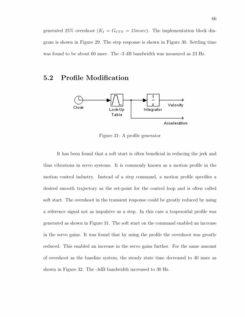
66
generated 25% overshoot (KI = GV TN = 15msec). The implementation block dia-
gram is shown in Figure 29. The step response is shown in Figure 30. Settling time
was found to be about 60 msec. The -3 dB bandwidth was measured as 23 Hz.
5.2 Profile Modification
Figure 31: A profile generator
It has been found that a soft start is often beneficial in reducing the jerk and
thus vibrations in servo systems. It is commonly known as a motion profile in the
motion control industry. Instead of a step command, a motion profile specifies a
desired smooth trajectory as the set-point for the control loop and is often called
soft start. The overshoot in the transient response could be greatly reduced by using
a reference signal not as impulsive as a step. In this case a trapezoidal profile was
generated as shown in Figure 31. The soft start on the command enabled an increase
in the servo gains. It was found that by using the profile the overshoot was greatly
reduced. This enabled an increase in the servo gains further. For the same amount
of overshoot as the baseline system, the steady state time decreased to 40 msec as
shown in Figure 32. The -3dB bandwidth increased to 30 Hz.

67
Figure 32: Response of the system using a profile

68
5.3 Nonlinear PI Control
A proportional integral(PI) controller is generally implemented in the industry
to control the velocity of a motor. The conventional PI controller can be described
as:
u = KP (e+KI
∫e dt) (5.1)
where, e and∫e represent the error, and the integral of error. KP is the proportional
gain and KI is the integral time constant. The very simplicity of the PI controller
which makes it attractive, also becomes a liability when it comes to performance.
Since the digital era began various attempts have been made to enhance it with
methods like gain scheduling and other nonlinear means. But the methods often
turned out to be problem dependent and not easily repeatable for different problems.
Han proposed a fundamental change in the way the nonlinear function is designed.
Based on the conventional PI controller, a nonlinear PI controller is described as
u = KP [fal(e, αP , δP ) +KI(fal(e, αI , δI)] (5.2)
where, e and∫e are the same as in PI and fal(∗) is a nonlinear function which is
defined as
fal(x, α, δ) =
|x|α sign(x), |x| > δ
xδ1−α , |x| ≤ δ
δ > 0 (5.3)
The reason, the nonlinear controller performs better is that, when 0 < α < 1, it
provides higher gain when the error is small and lower gain when error is large. A
plot of the function fal(∗) vs e is shown in Figure 33.

69
Figure 33: Plot of nonlinear function vs. error
Figure 34: Block diagram of the plant using an NPI Controller

70
It was shown in [22] that such a control law provides better disturbance rejec-
tion and faster command response. Due to the 900 lag associated with the integral
control, it is seldom used in dealing with resonance problem of concern here. In this
research, however, the nonlinear integral control along with nonlinear proportional
control greatly improved the performance of the plant. It is known that in general an
integral term causes saturation, which leads to an overshoot in the transient region.
However, by using the fal function shown above, gains can be chosen to be higher
when the error is small and relatively lower when the error is large. This configuration
Figure 35: Command response using a NPI controller
enabled an increase in the servo gains, which improved the system transient time and
offered higher disturbance rejection. Motor velocity using the NPI configuration is

71
plotted in Figure 35. When the nonlinear control was used along with the soft start it
gave a smoother response and good disturbance rejection and was found to be better
than most existing techniques. It can be seen from Figure 35 that the settling time
was reduced to 14 msec with the additional advantage of no overshoot in the motor
velocity. The -3dB bandwidth was found to increase to 72 Hz.
5.4 Acceleration Feed-forward with Nonlinear Servo
gains
Secondary output from the profile generator shown in Figure 31 is the accel-
eration command. Unlike the actual acceleration, or the observed acceleration, the
command acceleration is free of errors in differentiation or observation. This acceler-
ation command from the profile is fed forward, scaled by a gain KFF , to the control
signal, as shown in Figure 36. When acceleration feed-forward is applied to the base-
Figure 36: Block diagram of motor with Acceleration Feed-forward and Nonlineargains
line system, it improved the settling time of system. When acceleration feed-forward
was used with NPI, best results were obtained. NPI gave good disturbance rejection,
and the feed-forward signal improved the settling time of the response. It can be seen

72
Figure 37: Command response using Acceleration Feed-forward and NPI
73
from the figure that the settling time was reduced to 10 msec, and the bandwidth
was measured to be 82 Hz, which is almost 4 folds increase over the baseline system.
5.5 Discrete Time Optimal Control
Time optimal control(TOC) is an established technique in control. It origi-
nated in servo control design problems in 1950s, where heuristic arguments were made
regarding the optimality. It was extended to the second order system y + 2ζy + y =
ϕ(y, y), where ϕ(y, y) is a switching function of values ±1. Based on the Pontrya-
gin’s principle, the existence of a solution, the uniqueness of the solution and number
of switches in control signal were proved for time optimal control of a linear time
invariant continuous plant.
From the engineering perspective, the instant switching between extreme values
in the control signal required by the TOC is often neither feasible, because of the
physical limits on how fast a control signal can change, nor desirable because of the
stress it puts on the control actuators. On the other hand, the research continues
in development of methodology on determining switching surfaces for various plants.
Recently Z. Gao et al. have extended the TOC technique to non-unity gain plants.
A non unity gain second order plant is denoted by
x1 = x2
x2 = Ku
(5.4)

74
The optimal control algorithm to the non-unity gain plant is given as [15]:
δ = hKR,
δ1 = h2KR,
z1 = x1 + hx2,
z2 = x2,
g(z) =
z2 + z1
h, |z1| ≤ δ1
z2 − sign(z1)KR2
(h−√
8|z1|KR
+ h2), |z1| > δ1
u(z1, z2) = −R ∗ sat(g(z), hKR)
(5.5)
where, sat is defined as:
sat(a, b) =
sign(a), |a| > b
ab, |x| ≤ b
(5.6)
The parameters in the above set of equations are: K is the overall gain of the plant,
Figure 38: DTOC based implementation of the plant
R is the limit value of the control signal, h is the sampling rate, and u is the control
signal driving the plant. The control scheme defined in Eqs. 5.5 and 5.6 is the Discrete
Time Optimal Control law(DTOC) for a non-unity gain plant. For more information
on DTOC see [15]. This technique was used here to study the performance of the test
unit under consideration. Instead of position and velocity as the two states, velocity

75
and acceleration were treated as the two states while applying the control signal. The
implementation block diagram is shown in Figure 38. Results obtained using a DTOC
are plotted in Figure 39. Results were not as good as that of NPI with Acceleration
Feed-forward.
Figure 39: Command response using a DTOC
5.6 Active Disturbance Rejection Control
It is well known that integral control helps to suppress steady state error, re-
duce the transient time and improve disturbance rejection in a plant. However, it
also brings inevitable lag, which could destabilize the closed loop system. An alter-

76
native to dealing with disturbances and steady state errors was proposed by Prof.
Han in the form of a unique nonlinear observer designed to estimate disturbances.
By estimating an extended state which represents the internal dynamics and exter-
nal disturbances of the physical system it is possible to reduce the system to a pure
second order plant which can be controlled using a PD controller. This observer is
model independent. By choosing the nonlinear function carefully, we can estimate
the internal and external uncertainties and remove them using the modified control
signal. The final structure involving the modified control signal, Nonlinear Propor-
tional Derivative(NPD) control and Extended State Observer(ESO) form the Active
Disturbance Rejection Control(ADRC) .
5.6.1 Extended State Observer
The governing equation for the second order motor model is given by:
JM xM = −bSxM −KSxM + bSxL +KSxL +W +KTu (5.7)
Which can be rewritten as
xM = f +1
JM
∗ (−bSxM −KSxM +KTu) (5.8)
where, f is referred to as generalized disturbance which include external disturbances
W and internal plant dynamics. Although ESO may be designed without any infor-
mation about the plant; available plant dynamics may be incorporated to simplify
the tuning of ESO. Eq. 5.8 is a second order model. Applying the ESO to this model

77
we get
z1 = z2 −β01fal(e)
z2 = z3 −β02fal(e)− (bSz2+KSz1−KT u)JM
z3 = −β03fal(e)
(5.9)
where, e = z−xM and fal(.) is the nonlinear function given in Eq. 5.3. As z1 and z2
estimate the states of the plant in Eq. 5.7, the state z3 estimates the combination of
external disturbances and plant uncertainties f . If we can estimate the disturbance
and actively eliminate it from the plant as shown in Figure 40 the plant reduces to a
second order system which can be easily controlled using a PD controller.
The name ADRC comes from its ability to actively detect and compensate
the total disturbance, which lumps together the effects of internal and external dis-
turbances. The former comes from the system dynamics and can be assumed to be
unknown. The latter represents the external forces applied to the system that needs
to be compensated by the control signal.
Applying ESO to plant in Eq. 5.7, it is reduced to a double integrator control
problem which can be easily controlled using a PD controller. Using the profile
generator to generate the desired trajectory a nonlinear PD controller is used. This
overall architecture is called ADRC. The control law takes the form u(t) = u0(t) −
z3(t) ∗ JM/KT with
u0(t) = β1fal(x1 − z1) + β2fal(x2 − z2) (5.10)
The output position and control signal are fed to the ESO and the outputs of the
ESO are used to apply the modified control signal to the plant and feedback. The sim-
ulation block diagram is shown in Figure 40. Simulation results are shown in Figure

78
Figure 40: Block diagram for ADRC structure
Figure 41: Simulation result using ADRC

79
41. The controller performed extremely well in the presence of external disturbances
and model parameter variations because it does not overly depends on the model of
the plant. However, a major problem in implementation was the high sampling rate
required for the ESO to estimate the states and the disturbance. In the simulation
study it was found that it was difficult to estimate the states with sampling rate less
than 100 KHz. However, the drive on the test unit was limited to a sampling rate of
4 KHz, which made implementation difficult under the present circumstances. It was
found that the key to this design approach was the ESO. Once the ESO was properly
tuned the nonlinear PD gains were usually straightforward since they had the same
linear PD control intuition.
5.7 Single Parameter Tuning
The Extended State Observer(ESO) is an excellent observer, and it forms the
core part of the Active Disturbance Rejection Control(ADRC). However, the number
of tuning parameters involved (9 in case of a 3-state observer) makes the tuning
process highly cumbersome. In addition, since there is no knowledge between design
objectives and these parameters, it is difficult to determine whether or not the final
tuning result is optimal. Based on this difficulty, Z. Gao recently developed a linear
ESO, which can be tuned using a single parameter. This technique aims to reduce
the transfer function of a plant to a unit gain and unit bandwidth form(UGUB) [21].
The pre-designed controller for the UGUB is simply numerically scaled for the plant.
The controller parameterization makes all control parameters to be functions of a

80
single variable, the loop gain bandwidth, which can be easily tuned.
5.7.1 Linear Extended State Observer
Due to the complexity of the ESO and difficulty of its implementation on the
motion control set-up, the motion control model was simplified to represent it as a
first order model corrupted by external disturbances. Reconsider the Eq. 5.7 with
the state being velocity. The governing equation for the first order motor model is
given by:
JM VM = −bSVM +W +KTu (5.11)
Which can be rewritten as
x =1
JM
(−bSx+W +KTu− boJMu) + bou = f + bou (5.12)
This is the state space form of Eq. 5.11 with the state x representing the velocity of
the plant VM . f is referred to as a generalized disturbance, which includes external
disturbancesW and internal plant dynamics. The basic idea is that if we can somehow
obtain an estimate of f , f , then the control law u = −f+uo
boreduces the plant to
x = (f − f) + uo, which is a unit-gain single integrator control problem with a
disturbance of (f − f).
Rewriting the plant in Eq. 5.12 in state space form
x1 = x2 + bou
x2 = h
(5.13)
where, x2 = f is added as an augmented state, and h = f is seen as an unknown
disturbance. Now f can be estimated using a state observer based on the state space

81
model
x = Ax+Bu+ Eh
y = Cx
(5.14)
where,
A =
0 1
0 0
, B =
bo
0
, C =
[1 0
], E =
0
1
(5.15)
Now the state space observer, denoted as the Linear Extended State Ob-
server(LESO) can be constructed as
z = Az +Bu+ L(y − y)
y = Cz
(5.16)
where, L is the observer gain vector given by
L = [β1 β2]T (5.17)
Define ei = xi − zi, i = 1, 2; subtract Eq. 5.16 from Eq. 5.14, the error is :
e = (A− LC)e+ Eh
= Aee+ Eh
(5.18)
where Ae = A− LC =
−β1 1
−β2 0
.
5.7.2 Parameterization of Linear Extended State Observer
If h is bounded and if all the roots of the characteristic polynomial are in the
left half of the s-plane, then LESO is BIBO stable and the observer will track all the
states as z1 → y, z2 → f . The characteristic polynomial of Ae is
λ = s2 + β1s+ β2 (5.19)

82
Figure 42: Observed velocity using LESO

83
For simplicity if we assume that both the eigen values are same then
λ = s2 + β1s+ β2 = (s+ ωo)2 (5.20)
then, β1 = 2ωo and β2 = ω2o . Here ωo has a specific meaning: it is the bandwidth of the
observer. The larger the ωo, the quicker the disturbance is observed and cancelled by
the controller. In actual practice, this bandwidth is limited by hardware such as noise
and sampling rate. Plot of actual velocity and the observed velocity for the motion
control plant using LESO parameterization is shown in Figure 42. The observed
velocity is immune to measurement noise and tracks the actual velocity closely.
5.7.3 Controller Parameterization
Once the observer is built and well tuned, the output of the observer z1 and
z2 will track y and f(t, y, w) respectively. The objective is to actively eliminate the f
from the plant and reduce it to a single integrator plant. The control law is given by
u =−z2 + uo
bo(5.21)
as z2 → f the plant equation reduces to
y = uo (5.22)
The feedback control law can be
u = kpe (5.23)
where kp is the proportional gain. A single proportional gain is sufficient under
this configuration as the extended state dynamically eliminates the effect of external

84
disturbances. In terms of the error the plant equation becomes
y = u = kpe (5.24)
In terms of the setpoint r Eq. 5.24 reduces to
y = kp(r − y) (5.25)
taking the laplace transform of Eq. 5.25 we get
sY (s) = kpR(s)− kpY (s) (5.26)
the closed loop transfer function from setpoint r to plant velocity y reduces to
G(s) =Y (s)
R(s)=
kp
s+ kp
(5.27)
The controller tuning reduces to tuning a single parameter kp tuning, where, kp has
a specific meaning: it is the bandwidth of the controller ωc. The larger the kp, faster
the disturbance rejection. In actual practice however, this is limited by hardware.
5.7.4 Linear Active Disturbance Rejection Control
When the ESO is replaced by LESO, and the controller reduced to a single pa-
rameter bandwidth controller the ADRC architecture reduces to a Linear ADRC(LADRC).
Once the observer gains are designed, the primary control objective of the LADRC
comes down to tuning the controller bandwidth by modifying ωc. Maximize the ωc
to achieve greatest performance until noise levels and/or oscillations in the control
signal are close to tolerance limits. The implementation block diagram of a LADRC
is shown in Figure 43. Hardware results for the plant using a LADRC are shown in

85
Figure 43: Simulation block diagram using LADRC
Figure 44: Response of the plant using Single Parameter Tuning

86
Figure 44. LADRC with the soft start gave a smooth response and good disturbance
rejection and was found to have least noise content when compared to other tech-
niques that were implemented in hardware. It can be seen from Figure 44 that the
settling time was found to be 14 msec with the additional advantage of no overshoot
in the motor velocity. The -3dB bandwidth was found to be 72 Hz. The largest
advantage offered by this technique was its simplicity and ease of application. The
practical aspects of the tuning parameters involved makes this technique most user
friendly.
5.8 Multiresolution Wavelet Controller
Most control applications in industries still rely on a traditional PID controller.
PIDs have been a phenomenon in industry due to their intuitiveness and simplicity
of tuning. In general, a PID controller takes as its input the error(e), then acts on
the error so that a control signal, u, is generated. Gains KP , KI and KD are the
Proportional, Integral and Derivative gains used by the system to act on the error,
integral of the error, and derivative of the error respectively. In terms of frequency
content, the proportional and integral terms tend to capture the low frequency in-
formation of the error signal and derivative captures the high frequency information
of the signal. In a similar manner a multiresolution wavelet controller(MWC) gener-
ates a control signal based on the decomposition of the error signal into its high, low
and intermediate scale signal components, using the multiresolution decomposition
property of the wavelets. Error signals obtained using high scale decomposition are

87
called Approximations, and those obtained using low scale decomposition are called
Details. Each of these signal components tend to capture certain range of frequency
components contained in the original error signal. For example, the high scale signal
captures the low frequency information, low scale signal captures the high frequency
information and the intermediate scale signals capture the intermediate frequency
signal contained in the original error signal. Each of these components are multiplied
by their respective gains, and then added together to generate the control signal u.
This configuration of combining the signals to generate the control signal makes the
MWC analogous to a Proportional-Integral-Derivative(PID) controller. The block
Figure 45: Simulation response using a Multiresolution Wavelet Controller
diagram for implementation of the MWC for the motor is same as Figure 13 except

88
that the plant model is replaced by Figure 4. Results obtained using simulation are
shown in Figure 46. In the case where disturbance was applied both plants had zero
steady state error; however, MWC approached zero at a relatively faster rate. And
it exhibited far better noise rejection than the PI controller as can be seen in Fig-
ure 46. Noise is an important factor that effects control system performance. It is
an established fact that noise restricts the bandwidth of the control system and re-
duces system stability. Therefore using a MWC offers distinct advantage of improving
system bandwidth and stability.
Figure 46: Effect of noise during steady state response
Unlike a PID controller, which has three tuning parameters (gains) a MWC
can have two or more parameters based on the level of decomposition of the error

89
signal. Furthermore, MWC is very intuitive, easy to understand and tune. For a plant
corrupted with high amount of measurement noise, MWC can be used to generate
low and high frequency components and then as noise is high frequency component
of the error signal, gain corresponding to the high frequency component can be set
to zero. In a similar way higher gains have to be assigned to the lower frequency
components of the MWC in order to increase the disturbance rejection of the plant.
5.9 Summary of Results
Although results for each of the techniques are disscussed in their relevant sec-
tion, an overall comparison and their tuning parameters are shown in this section.
Nonlinear PI, acceleration feedforward and LADRC produced good results on the test
setup and are plotted for comparion in Figure 47. Although ADRC and Multireso-
lution controller also gave good results they were not implemented on the test setup
due to complexity of the algorithm and the memory and hardware limitations of the
servo drive. When the nonlinear control was used along with the soft start it gave
a smoother response and good disturbance rejection. The settling time was reduced
to 14 msec with the additional advantage of no overshoot in the motor velocity. The
-3dB bandwidth was found to increase to 72 Hz. When acceleration feed-forward was
used along with NPI, best results were obtained in terms of system bandwidth. NPI
gave good disturbance rejection, and the feed-forward signal improved the settling
time of the response. The settling time was reduced to 10 msec, and the bandwidth
was measured to be 82 Hz, which is almost 4 folds increase over the baseline system.

90
Figure 47: Comparison of results

91
It can be seen that this controller produced the smallest error signal compared to
all other techniques. LADRC with the soft start gave a smooth response and good
disturbance rejection and was found to have least noise content when compared to
other techniques that were implemented in hardware. The settling time was found to
be 14 msec with the additional advantage of no overshoot in the motor velocity. The
-3dB bandwidth was found to be 72 Hz. The biggest advantage of this technique was
its simplicity and ease of application. The practical aspects of the tuning parameters
involved, makes this technique most user friendly.

92
Table 4: Parameters and comparison of results of different techniques
DTOC LADRC MWCh (sec) 2.5 ∗ 10−4 2.5 ∗ 10−4 2.5 ∗ 10−4
R 4096 x xK 8192 x x
KH x x 0.025KL x x 0.0
KM 1 x x 0.2KM 2 x x 0.2Kp x 6 xWo x 128 xbo x 4096 x
SSTime(Sec) 30 14 32BW(Hz) 43 72 40
Baseline Profile NPI NPI with AFF ADRCh (sec) 2.5 ∗ 10−4 2.5 ∗ 10−4 2.5 ∗ 10−4 2.5 ∗ 10−4 10−4
KP 2.5 4.5 15 12 0.1KI (msec) 15 15 45 20 x
KD x x x x 10−8
KFF x x x 0.43 xαP x x 0.9 x 0.35αI x x 0.9 x xαD x x x x 0.5δP x x x x 10−6
δI x x x x xδD x x x x 10−6
α1 x x 0.9 x 1α2 x x 0.9 x 0.5α3 x x x x 0.25β1 x x x x 2000β2 x x x x 98000β3 x x x x 106
δ1 x x x x 9*10−4
δ2 x x x x 10−4
δ3 x x x x 0.0079SSTime(Sec) 60 40 14 10 27
BW(Hz) 23 30 72 82 48

CHAPTER VI
CONCLUSIONS AND FUTURE WORK
A novel controller based on multiresolution decomposition using wavelets called
the Multiresolution Wavelet Controller was developed. This controller is similar to a
Proportional-Integral-Derivative controller in principle and application. The output
from a control system represents the cumulative effect of uncertainties such as mea-
surement noise, frictional variation and external torque disturbances, which manifest
at different scales. The wavelet is used to decompose the error signal into signals at
different scales. These signals are then used to compensate for the uncertainties in
the plant. This controller is applied to different industrial applications to validate
the control scheme. A scheme to compute DWT in real-time using a signal pipeline
architecture is also developed.
Wavelet transform is performed on a bunch of data after it is made available
to the processing engine on account of the non-causal nature of the wavelets. As
93

94
control systems require real-time signal processing in order to operate in real-time,
wavelets have had limited applications in controls. In order to perform multi-level
decomposition for real time operation, a novel pipeline data architecture is developed.
This architecture not only provides wavelet transform in real-time, it also resolves the
issue of ill-conditioned data at the boundaries.
A scheme to generate low noise differential signal using wavelets is also devel-
oped. Wavelet transforms are investigated for their ability to solve industrial control
issues such as noise, disturbance, and improving loop bandwidth. Different schemes
to improve existing controllers using wavelet differentiator and wavelet denoising are
proposed.
Linear and non-linear algorithms including Profile modification, NPI, LADRC
and TOC to solve low frequency mechanical resonance are proposed and applied on
an industrial setup.
6.1 Future Work
A Novel control scheme using wavelets is developed in this research. A lot of
different aspects related to this controller can be considered for future work. Further
research is needed to investigate the stability of the controller. Some preliminary
results on tuning the MWC are given. Further work needs to be done to investigate
the tuning of both integrating and non-integrating plants. An important feature
that may be added to the MWC is to investigate integration as part of the wavelet
decomposition. Although integration may be added as an external feature to the

95
MWC, it will be desirable to investigate how integration may be performed using
wavelets.

BIBLIOGRAPHY
[1] D. B. Percival and Andrew T. Walden, Wavelet methods for Time Series Analysis,
Cambridge University Press, 2000.
[2] G. Ellis, Control System Design Guide 2nd Ed. , Academic Press, 2000.
[3] G. Ellis and R.D. Lorenz, Resonant Load Control Methods for Industrial Servo
Drives, IEEE Industrial Application Society 2000 Annual Meeting and World
Conference on Industrial Applications of Electrical Energy, Oct. 8-12, 2000.
[4] G. Ellis and Z. Gao , Cures for Low-Frequency Mechanical Resonance in Industrial
Servo Systems, ISA Emerging Technology Conference, September 12, 2001.
[5] G. Stephanopoulos, O. Karsligil, and M. Dyer, Multi-scale aspects in model-
predictive control Journal of Process Control, 10(2000) pp. 275-282.
[6] G.W. Younkin, W.D. McGlasson, and R.D. Lorenz, Considerations for low-inertia
AC drives in machine tool axis servo applications IEEE Trans. on Ind. Appl.,
Vol 27, No 2, March/April 1991, pp. 262-268.
[7] H. Wertz, F. Schtte, Self-tuning speed control for servo drives with imperfect
mechanical load IEEE Industrial Application Society 2000 Annual Meeting and
World Conference on Industrial Applications of Electrical Energy, Oct. 8-12,
2000.
96

97
[8] I. Daubechies, Ten lectures on Wavelets SIAM, CBMS-NSF Regional Conference
Series in Applied Mathematics, 1992.
[9] J. Deur, A comparative study of servosystems with acceleration feedback IEEE
Industrial Application Society 2000 Annual Meeting and World Conference on
Industrial Applications of Electrical Energy, Oct. 8-12, 2000.
[10] J.K. Kang and S.K. Sul, Vertical-vibration control of elevator using estimated
car acceleration feedback compensation IEEE Trans. on Ind. Elec., Vol. 47, No.
1, Feb 2000, pp. 91-99.
[11] P. Schmidt and T. Rehm, Notch filter tuning for resonant frequency reduction in
dual inertia systems Proc. of IEEE IAS, Oct. 3-7, 1999, Phoenix, pp. 1730-1734.
[12] P.B. Schmidt and R.D. Lorenz, Design Principles and Implementation of Accel-
eration Feedback to Improve Performance of DC Drives, IEEE Trans. on Ind.
Appl., May/June 1992, pp. 594-599.
[13] R.H. Welch, Mechanical Resonance in a Closed-Loop Servo System: Problems
and Solutions Tutorial from Welch Enterprises, Oakdale, MN.
[14] R. Dhaouadi, K. Kubo, and M. Tobise, Analysis and compensation of speed drive
systems with torsional loads IEEE Trans. on Ind. Appl., Vol 30, No 3, May/June
1994, pp. 760-766.
[15] S. Hu, On high performance servo control solutions for hard disk drive Doctoral
Thesis, CSU, April 2001.

98
[16] S.G. Mallat and G. Zhang, Matching Pursuits with Time-Frequency Dictionaries.
IEEE Transactions on Signal Processing, Vol 41, pp. 3397-415.
[17] S. Ungarala and B. R. Bakshi, Multiscale Bayesian Estimation and Data Rec-
tification Wavelets in Signal and Image Processing, A. Petrosian and F. Meyer,
eds., Kluwer Academic Publishers, New York, NY, In print, (2001).
[18] S. Vukosavic and M. Stojic, Suppression of Torsional Oscillations in a High-
Performance Speed Servo Drive, IEEE Trans. on Ind. Elec, Vol 45, No 1, Feb
1998, pp. 108-117.
[19] Y. Hori, H. Sawada, and Y. Chun, Slow Resonance ratio control for vibration
suppression and disturbance rejection in torsional system, IEEE Transactions on
Industrial Electronics, vol. 46, No. 1, pp.162-168, Feb, 1999.
[20] Y.M. Lee, J.K. Kang and S.K. Sul, Acceleration feedback control strategy for
improving riding quality of elevator system Proc. of IEEE IAS (Phoenix), 1999,
pp. 1375-1379.
[21] Z. Gao Scaling and bandwidth-parameterization based controller-tuning, Pro-
ceedings of the 2003 American Control Conference, June 2003, pp. 4989-4966.
[22] Z. Gao, From linear to nonlinear control means: A practical progression, ISA
Emerging Technology Conference, To appear in ISA Transactions, September 12,
2001.
[23] Z. Gao and T. A. Trautzsch, A stable self-tuning fuzzy logic control system

99
for industrial temperature regulation IEEE Industrial Application Society 2000
Annual Meeting, Rome, 2000.
[24] Z. Gao, Y. Huang and J. Han, An Alternative Paradigm for Control System
Design, Proc. of IEEE conference on Decision and Control, 2001, pp. 4578-4585.
[25] Z. R. J. Eucker and Z. Gao, A Novel Self-Tuning Control Design Approach
for Industrial Applications, IEEE Industrial Application Society 2000 Annual
Meeting and World Conference on Industrial Applications of Electrical Energy,
Oct. 8-12, 2000.

APPENDIX
APPENDIX

101
A. MWC CODE
In this appendix a ”c” code for implementation of Multiresolution Wavelet Con-
troller on a motion control setup are given. The code needs to be compiled using a
’TURBO C’ programing compiler. Some of the header files related to the drive have
to be included during compilation. If the number of decomposition levels, and the
wavelet filters need to be changed for testing purposed this has to be done during
compile-time, as they are hard coded. However, this will just need some changes in
the global variables and memory allocation to arrays. The gains of the controller can
be tuned during run-time. It is often advisable to assign zero gain to the highest
signal component to provide good amount of noise rejection. The midlevel compo-
nents may be tuned to provide damping, to increase the transient time and the low
frequency component may be tuned aggressively, to track the changes in setpoint and
provide greater immunity to disturbances.
/ ∗ ∗ ∗ ∗ ∗ ∗ ∗ ∗ ∗ ∗ ∗ ∗ ∗ ∗ ∗ ∗ ∗ ∗ ∗ ∗ ∗ ∗ ∗ ∗ ∗ ∗ ∗ ∗ ∗ ∗ ∗ ∗ ∗ ∗ ∗ ∗ ∗ ∗∗
”C” Code for implementation of Multiresolution
Wavelet Controller for Servo Motor Postion Control
∗ ∗ ∗ ∗ ∗ ∗ ∗ ∗ ∗ ∗ ∗ ∗ ∗ ∗ ∗ ∗ ∗ ∗ ∗ ∗ ∗ ∗ ∗ ∗ ∗ ∗ ∗ ∗ ∗ ∗ ∗ ∗ ∗ ∗ ∗ ∗ ∗ ∗ ∗ ∗ /
#include <stdio.h>
#include <math.h>
#include <stdlib.h>
#include <dos.h>

102
#include <conio.h>
#define number 1000
#define pi 3.141592653589793
/ ∗ ∗ ∗ ∗ ∗ ∗ ∗ ∗ ∗ ∗ ∗ ∗ ∗ ∗ ∗ ∗ ∗ ∗ ∗ ∗ ∗ ∗ ∗ ∗ ∗ ∗ ∗ ∗ ∗ ∗ ∗ ∗ ∗ ∗ ∗ ∗ ∗ ∗∗
Declaration of global functions
∗ ∗ ∗ ∗ ∗ ∗ ∗ ∗ ∗ ∗ ∗ ∗ ∗ ∗ ∗ ∗ ∗ ∗ ∗ ∗ ∗ ∗ ∗ ∗ ∗ ∗ ∗ ∗ ∗ ∗ ∗ ∗ ∗ ∗ ∗ ∗ ∗ ∗ ∗ ∗ /
unsigned long read 7166();
void Wavelet decomposition(double *Signal, double *DecomposedSignal,
double *LowFilter, double *HighFilter);
double Wavelet Decrec(double *DecomposedSignal, double *LowFilterRec,
double *HighFilterRec, int level);
double Wavelet Apprec(double *DecomposedSignal, double *LowFilterRec);
void Convolution(double *Signal, double *Filter, double *Convolved Signal,
int SignalLength);
void Upsampling(double *Signal, double *SampledSignal, int SignalLength);
void DownSampling(double *Signal, double *SampledSignal, int SignalLength);

103
static const long length of filter=8;
static const long Signal length=64;
static const long NoOfLevels=5;
static const long DecomposedSignalLengths[] = {64, 35, 21, 14, 10, 8, 8};
static const long RecSignalLengths[] = {8, 10, 14, 21, 35, 71};
static const long RecSignalIndex[]= {88, 80, 70, 56, 35, 0};
/ ∗ ∗ ∗ ∗ ∗ ∗ ∗ ∗ ∗ ∗ ∗ ∗ ∗ ∗ ∗ ∗ ∗ ∗ ∗ ∗ ∗ ∗ ∗ ∗ ∗ ∗ ∗ ∗ ∗ ∗ ∗ ∗ ∗ ∗ ∗ ∗ ∗ ∗ ∗ ∗ ∗ ∗ ∗ ∗/
void main(){
double Kp, Kd, Ki, h;
double KA5, KD5, KD4, KD3, KD2, KD1,ControlSignal=0;
double ErrorBufferSignal[64];
double Signal[64];
double Convolved Signal[100];
double DecomposedSignal[100];
double ReconstructedSignal[6];
double LowFilter[] = {-0.0106, 0.0329, 0.0308, -0.1870, -0.0280, 0.6309,
0.7148, 0.2304};
double HighFilter[] = -0.2304, 0.7148, -0.6309, -0.0280, 0.1870, 0.0308,
-0.0329, -0.0106;
double LowFilterRec[] = 0.2304, 0.7148, 0.6309, -0.0280, -0.1870, 0.0308,
0.0329, -0.0106;
double HighFilterRec[] = -0.0106, -0.0329, 0.0308, 0.1870, -0.0280, -0.6309,

104
0.7148, -0.2304;
int index,Index1;
double y, y0, ysp=0, V max, e, e 1, e dot, e integral, t sec=0, t1, u, out,
ysp buffer=0,scale, y buffer=0;
long t previous, t current, position;
int time count;
int i=0, k, first=1, flag=0;
char buff[10];
double time[number],control[number],feedback[number],
error[number],error dot[number];
FILE *fp, *Stream;
init DAC();
for (i=0; i<100; i++ )
DecomposedSignal[i]=0;
for (i=0; i<6; i++ )
ReconstructedSignal[i]=0;
for (i=0; i<number; i++ ){
time[i]=0;
control[i]=0;

105
feedback[i]=0;
error[i]=0;
error dot[i]=0;
}
for (index =0; index<Signal length; index++)
ErrorBufferSignal[index]=0.0;
fp = fopen(”wav1.out”,”w”); /∗ open file for saving data ∗/
if (fp==NULL) {
printf(”Can’t create the output file wav1.out\ n”);
exit(1);
}
Stream = fopen(”wav.out”,”w”); /∗ open file for saving data ∗/
if (Stream==NULL) {
printf(”Can’t create the output file wav.out\n”);
exit(1);
}
printf(”\ n Input how many revolutions to go [default 1]: ”);
gets(buff);
if (strlen(buff) == 0) y0=1;

106
else
y0 = atof(buff);
V max= 7.0;
Kp = 2.8;
Kd = 1.5;
Ki = 0.0001;
printf(”\ n KA5 [default 7.5]: ”); /∗ 7.5, 30, 30 for 5 level decomposition∗/
gets(buff);
if (strlen(buff) == 0) KA5 = 7.5;
else
KA5 = atof(buff);
printf(”\ n KD5 [default 30]: ”);
gets(buff);
if (strlen(buff) == 0) KD5 = 30;
else
KD5 = atof(buff);
printf(”\ n KD4 [default 30]: ”);
gets(buff);
if (strlen(buff) == 0) KD4 = 30;
else

107
KD4 = atof(buff);
printf(”\ n Program running... \ n”);
printf(”\ n Press any key to exit. \ n”);
init 7166();
init 8254();
i=0;
e 1 = 0;
e integral = 0;
t1 = 3*pi*y0/V max;
t previous = read 8254();
delay(15);
while(kbhit()) {
for (k=0; k<10; k++) {
t current=read 8254(); /∗ decide step size ∗/
if (t current¿t previous) t previous+=65536;
time count=(int)(t previous-t current);
h=(double)time count/1193180.0;
if (first) h = 0.001;
t previous=t current;
t sec+=h;

108
if (t sec ¡= t1/3) ysp = 3*V max/t1/2*t sec*t sec;
else
if (t sec¡= 2*t1/3) ysp = V max * t1/6 + V max * (t sec-t1/3);
else
if (t sec¡=t1) ysp = V max * t1/2
+((t sec-2*t1/3)*t1-(t sec*t sec-4*t1*t1/9)/2)*3*V max/t1;
else
ysp = 2*V max*t1/3;
position = read 7166() - (unsigned long) 0x080800000;
y = (double)(position*2*pi/16000.0); /∗ obtain current position ∗/
e = ysp - y;
e integral = e integral + e;
e dot = e - e 1;
e 1 = e;
if (first) {
first = 0;
continue;
}
for (index=0; index ≤ 30;index ++){ /∗ Save the Error Buffer ∗/
ErrorBufferSignal[index]=ErrorBufferSignal[index+1];
ErrorBufferSignal[63-index]=ErrorBufferSignal[62-index];

109
}
ErrorBufferSignal[31]= e;
ErrorBufferSignal[32]= e;
for (index=0; index<Signal length;index ++){
Signal[index]=ErrorBufferSignal[index];
}
/∗ Decompose the signal ∗/
Wavelet decomposition(Signal, DecomposedSignal, LowFilter,
HighFilter);
switch(flag)
{
case 0:
{
ReconstructedSignal[0]=Wavelet Apprec(DecomposedSignal,
LowFilterRec);
flag=1;
}
break;
case 1:

110
{
ReconstructedSignal[1]=Wavelet Decrec(DecomposedSignal,
LowFilterRec, HighFilterRec,0);
flag=2;
}
break;
case 2:
{
ReconstructedSignal[2]=Wavelet Decrec(DecomposedSignal,
LowFilterRec, HighFilterRec,1);
flag=0;
}
break;
default:
break;
}
ControlSignal=KA5*ReconstructedSignal[0]+KD5*ReconstructedSignal[1]
+KD4*ReconstructedSignal[2];
if (ControlSignal > 3.5) ControlSignal = 3.5;
if (ControlSignal < -3.5) ControlSignal =-3.5;
out=5.0*ControlSignal/7.0+2.5;
DAC out(out);

111
} /∗ end of for clause ∗/
if ( i < number) { /∗ keep data for saving ∗/
fprintf(Stream, ”%f %f %f; \ n”, ReconstructedSignal[0],
ReconstructedSignal[1], ReconstructedSignal[2]);
time[i] = t sec;
control[i] = ysp;
feedback[i] = y;
error[i] = e;
error dot[i] = ControlSignal;
i = i + 1;
}
else
goto exit1;
}
exit1:
init DAC();
for (i=0; i¡number; i++ )
fprintf(fp,”%f %f %f %f %f; \n”,time[i], control[i],feedback[i],
error[i], error dot[i]);
fclose(fp);
fclose(Stream);

112
printf(”\ n Program completed \ n”);
} /∗ end of main ∗/
/ ∗ ∗ ∗ ∗ ∗ ∗ ∗ ∗ ∗ ∗ ∗ ∗ ∗ ∗ ∗ ∗ ∗ ∗ ∗ ∗ ∗ ∗ ∗ ∗ ∗ ∗ ∗ /
/∗ Function Decomposition ∗/
/∗ Given a Signal it computes wavelet coefficients ∗/
void Wavelet decomposition(double *Signal, double *DecomposedSignal,
double *LowFilter, double *HighFilter)
{
int index,index1, SIndex, tempIndex=0;
double AppSignal[80], DecSignal[80];
for (index=0; index<NoOfLevels; index++) {
Convolution(Signal, LowFilter, AppSignal, DecSignalLengths[index]);
Convolution(Signal, HighFilter, DecSignal, DecSignalLengths[index]);
DownSampling(AppSignal,Signal, DecSignalLengths[index+1]);
DownSampling(DecSignal,DecSignal, DecSignalLengths[index+1]);
for (SIndex=0; SIndex< DecSignalLengths[index+1]; SIndex++){
DecomposedSignal[SIndex+tempIndex]= DecSignal[SIndex];
}
tempIndex = tempIndex+DecSignalLengths[index+1];
}

113
for (SIndex=0; SIndex<DecSignalLengths[index+1]; SIndex++)
DecomposedSignal[SIndex+tempIndex]= Signal[SIndex];
}
/∗ Function for Reconstruction of Approximate Signal from coefficients ∗/
double Wavelet Apprec( double *DecomposedSignal, double *LowFilterRec)
{ int index, SIndex, subSIndex;
double appsignal[100],convolvedsignal[100],buffersignal[100];
for (index=0; index<RecSignalLengths[0]; index++)
appsignal[index]= DecomposedSignal[RecSignalIndex[0]+index];
for (index=0; index<NoOfLevels; index++){
Upsampling(appsignal,buffersignal, RecSignalLengths[index]);
Convolution(buffersignal,LowFilterRec,convolvedsignal,
2*ReconstructedSignalLengths[index]);
for (SIndex=0; SIndex<RecSignalLengths[index+1]; SIndex++){
appsignal[SIndex]=convolvedsignal[SIndex+length of filter-1];
}
}
return appsignal[31];
}

114
/∗ Function for Reconstruction of Detail Signal from coefficients ∗/
/∗ level=0 => Detail Signal at Nth Level, level=1 => Detail Signal at N-1 Level...
∗/
double Wavelet Decrec( double *DecomposedSignal, double *LowFilterRec,
double *HighFilterRec, int level)
{
int index, SIndex, SIndex2, SIndex3, SIndex4, tempIndex=0;
double detsignal[100],convolvedsignal[100],buffersignal[100];
tempIndex=RecSignalIndex[level+1];
for(SIndex=0; SIndex<RecSignalLengths[level] ; SIndex++){
detsignal[SIndex]=DecomposedSignal[SIndex+tempIndex];
}
for (SIndex3=level; SIndex3<NoOfLevels; SIndex3++){
Upsampling(detsignal,buffersignal, RecSignalLengths[SIndex3]);
if (SIndex3==level)
Convolution(buffersignal,HighFilterRec,convolvedsignal,
2*RecSignalLengths[SIndex3]);
else
Convolution(buffersignal,LowFilterRec,convolvedsignal,
2*RecSignalLengths[SIndex3]);

115
for(SIndex4=0; SIndex4<RecSignalLengths[SIndex3+1]; SIndex4++){
detsignal[SIndex4]=convolvedsignal[SIndex4+length of filter-1];
}
}
return detsignal[31];
}
/∗ Function to upsample a signal ∗/
void Upsampling(double *Signal, double *SampledSignal, int SignalLength)
{
int index;
for (index=0; index < SignalLength; index++){
SampledSignal[2*index+1]=Signal[index];
SampledSignal[2*index]=0;
}
}
/∗ Function to Compute convolution using a signal and a filter ∗/
void Convolution(double *Signal, double *Filter, double *Convolved Signal,
int signallength)
{
116
int index, SIndex;
double Buffer Signal[100], sum=0.0;
for (index=0; index <(signallength+2*length of filter) ; index++){
Buffer Signal[index]=0.0;
}
for (index=0; index<(signallength); index++){
Buffer Signal[length of filter+index]=Signal[index];
}
for (index=0; index<(signallength+length of filter); index++){
sum=0.0;
for (SIndex=0; SIndex < length of filter; SIndex++){
sum+= Filter[SIndex]*Buffer Signal[length of filter+index-SIndex];
}
Convolved Signal[index]=sum;
}
}
/∗ Function to downsample a signal ∗/
void DownSampling(double *Signal, double *SampledSignal, int SignalLength)
{

117
int index;
for (index=0; index<SignalLength ; index++){
SampledSignal[index] = Signal[index*2+1];
}
for (index=SignalLength; index<2*SignalLength ; index++){
SampledSignal[index] =0.0;
}
}
/ ∗ ∗ ∗ ∗ ∗ ∗ ∗ ∗ ∗ ∗ ∗ ∗ ∗ ∗ ∗ ∗ ∗ ∗ ∗ ∗ ∗ ∗ ∗ ∗ ∗ ∗/

118
B. WAVELET FILTERS
Table 5: Coefficients of Daubechies wavelet filters
l h for D(2) h for D(4) h for D(6) h for D(8)0 0.7071 0.4830 0.3327 0.23041 0.7071 0.8365 0.8069 0.71482 0.2241 0.4599 0.63093 -0.1294 -0.1350 -0.02804 -0.0854 -0.18705 0.0352 0.03086 0.03297 -0.0106
Coefficients of Symlet wavelet Filters
l h for Sym(2) h for Sym(4) h for Sym(6) h for Sym(8)0 0.7071 0.4830 0.3327 0.03221 0.7071 0.8365 0.8069 -0.01262 0.2241 0.4599 -0.09923 -0.1294 -0.1350 0.29794 -0.0854 0.80375 0.0352 0.49766 -0.02967 -0.0758
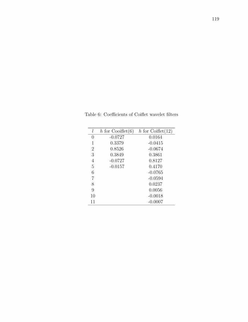
119
Table 6: Coefficients of Coiflet wavelet filters
l h for Cooiflet(6) h for Coiflet(12)0 -0.0727 0.01641 0.3379 -0.04152 0.8526 -0.06743 0.3849 0.38614 -0.0727 0.81275 -0.0157 0.41706 -0.07657 -0.05948 0.02379 0.005610 -0.001811 -0.0007

INDEX
Acceleration, 6, 16
Active Disturbance Rejection Control(ADRC),
76, 77, 81
Basis, 25
Best Basis, 40
Compliantly-coupled, 6
Conjugate, 26, 29, 30
Daubechies, 29, 35, 44
Decomposition, 25, 29, 30
Decomposition Analysis, 30
Decomposition Synthesis, 30
Detail, 29, 30
Disturbance, 11, 35, 52, 70
Extended State Observer(ESO), 76, 77
External disturbances, 3, 35
Feed-forward, 73
Feedback, 16
Fourier, 20
Fourier Transform, 21
Friction, 6, 7
Generalized Multiresolution Controller(GMC),
45, 46
Inertia, 6, 13
Instability, 6, 9, 64
Linerar Active Disturbance Rejection
Control(LADRC), 84
Measurement noise, 3
Mechanical damping, 7
Multiresolution, 24
Multiresolution Wavelet Controller(MWC),
v, 3, 18, 33, 35, 43, 45, 47, 86
Newton, 6
Nonlinear Control, 46
Observer, 16
Parameterization, 4, 79, 84
PID, 3, 8, 18, 32, 35, 49
Process dynamics, 3
120

121
Profile, 66
Profile modification, 4
Resonance, 2, 12, 13
Scaling Function, 30
Servo gains, 4
Stability, 15, 63
Sub-band Coding, 30
Time optimal control(TOC), 73
Torque, 6
Transfer function, 32
Trend, 29, 30
Wavelet Differentiator, 54
Wavelet Transform, v, 22, 23, 27, 32
Wavelets, 19, 23, 27, 30, 39