advanced dynamic spectrum 5g mobile networks employing ... · fair and regulated spectrum...
TRANSCRIPT

Advanced Dynamic spectrum 5G mobile networks Employing Licensed shared
access
Grant Agreement for: Collaborative project Project acronym: ADEL
Grant Agreement number: 619647

Deliverable D4.2 – Resource allocation schemes and optimized algorithms
ADEL ICT - 619647 Page 2 of 64
This project has received funding from the European Union’s Seventh Framework Programme for research, technological development and demonstration under grant agreement no. 619647.
Project Deliverable D4.2:
Resource allocation schemes and optimized algorithms
Contractual Date of Delivery: 01/06/2016
Actual Date of Delivery: 23/06/2016
Editors: Hicham Anouar (TCS)
Authors: Muhammad Majid Butt, Arman Farhang, Carlo Galiotto, Jasmina McMenamy, Nicola Marchetti ; Hicham Anouar, Dorin Panaitopol, Kostas Voulgaris, Nikolaos Taramas, Kostas Ntougias, George Papageorgiou
Work package title: WP4 – Licensed Shared Access resource allocation techniques
Work package leader: TCS
Contributing partners: UEDIN, AIT, TCS, TUDA, EUR, TCD, PTIN Nature O1
Dissemination level CO2
Version V1.3
Total Number of Pages: 63
File:
1 Nature of the Deliverable:
R = Report, P = Prototype, D = Demonstrator, O = Other 2 Dissemination level codes:
PU = Public PP = Restricted to other programme participants (including Commission Services) RE = Restricted to a group specified by the consortium (including the Commission Services) CO = Confidential, only for the members of the consortium (including the Commission Services)
Advanced Dynamic spectrum 5G mobile networks Employing Licensed shared access

Deliverable D4.2 – Resource allocation schemes and optimized algorithms
ADEL ICT - 619647 Page 3 of 64
Keywords:
Document Revision history
Version Date Send to Summary of main changes Approved by
V0.1 30/10/15 ALL Initial version with inputs from TCD, TUDA, and TCS
V0.2 25/11/15 ALL Complete input from TUDA V0.3 01/12/15 ALL Complete input from PTIN and TCS
V1 15/12/15 ALL Final version
V1.1 12/05/16 ALL Complete contribution from TCS
V1.2 27/05/16 ALL Complete contribution from TCD & TCS
V1.3 15/06/16 ALL Final editing of document
Abstract: This deliverable presents the details of the work performed on centralised and distributed resource allocation schemes and optimized algorithms. Analytical and numerical analysis and performance comparison are provided to identify the most promising resource allocation techniques for modern and future communication systems
Deliverable D4.2 – Resource allocation schemes and optimized algorithms
ADEL ICT - 619647 Page 4 of 64
Copyright
© Copyright 2014 – 2017, the ADEL Consortium
Consisting of:
Coordinator: Dr. Tharm Ratnarajah, University of Edinburgh (United Kingdom) - UEDIN
Participants:
Athens Information Technology (Greece) – AIT
Thales Communications and Security (France) - TCS
Technical University Darmstadt (Germany) - TUDA
Intel Mobile Communications GmbH (Germany) - IMC
EURECOM (France) - EUR
Trinity College Dublin (Ireland) - TCD
Portugal Telecom Inovacão SA (Portugal) – PTIN
This document may not be copied, reproduced, or modified in whole or in part for any purpose without written permission from the ADEL Consortium. In addition to such written permission to copy, reproduce, or modify this document in whole or part, an acknowledgement of the authors of the document and all applicable portions of the copyright notice must be clearly referenced.
This document reflects only the authors’ view. The European Community is not liable for any use that may be made of the information contained herein.
All rights reserved.

Deliverable D4.2 – Resource allocation schemes and optimized algorithms
ADEL ICT - 619647 Page 5 of 64
Executive Summary
This is the deliverable D4.2 Resource allocation schemes and optimized algorithms, FP7 project ADEL (ICT- 619647). This work was carried out as part of WP4: Licensed Shared Access resource allocation techniques. This deliverable relies on the work defined within tasks T4.1 and T4.2 detailed in the Description of Work.
In this deliverable, we have described the various developed centralised and distributed resource allocation solutions that outperform the existing state-of-the-art protocols in terms of energy efficiency, overhead, fairness, and convergence time, while taking into account the specific ADEL scenario. A brief summary of the deliverable is given below:
Centralised Resource Allocation Schemes
Fair and regulated spectrum allocation in licensed shared access networks : When the spectrum is made available by the incumbent, all the licensee operators (OP) compete for the resources. The L1 Algorithm assigns carrier bands to the operator. The algorithm performs spectrum allocation in a fair manner.
Spectrum auction resource allocation in small cell/Cloud RAN : Cloud-based massive-MIMO antennas and underutilized spectrum resources by the incumbent network are considered where the antennas cooperate to serve users of multiple virtual network operators (VNOs). Multiple VNOs share the antennas while they utilize orthogonally a pool of shared LSA spectrum resources. The approach in this work uses an auctioning mechanism to achieve the highest possible revenue while meeting minimum rate requirements that VNOs offer to their users.
Iterative convex approximation algorithm : A novel iterative convex approximation algorithm is proposed to efficiently compute stationary points for a large class of possibly nonconvex optimization problems. It is shown that the proposed framework not only includes as special cases a number of existing methods, for example, the gradient method and the Jacobi algorithm, but also leads to new algorithms which enjoy easier implementation and faster convergence speed.
Frequency agile centralized resource allocation algorithm : A simple centralised frequency allocation scheme is proposed which uses the frequency agility capabilities of the LSA licensees. The performance of this centralised algorithm is determined in terms of i) the probability of denying LSA licensees’ allocation requests, and ii) the probability of the LSA licensees having to return previously allocated spectrum in case an incumbent reclaims it afterwards. The work carried out, illustrates the benefits brought by the adoption of LSA, as well as the increased performance expected from the centralised algorithm.
Fair Opportunistic scheduler for real time traffic with reduced feedback size : Opportunistic scheduling of heterogeneous real time traffic in small cells scenario is considered where different eNBs share one or multiple LSA channels under the control of a central macro base station (BS). The performance of the new algorithm is compared to those of the proportional fair scheduling (PFS) and the Modified Largest Weighted Delay First (M-LWDF) algorithm.
Opportunistic beamforming for secondary users in Licensed Shared Access networks : A joint opportunistic beamforming and scheduling technique is proposed for the downlink of a secondary (Licensee) wireless system that coexists with a primary (Incumbent) one under the ADEL architectural setup. It is shown that the proposed technique exploits multi-user diversity to boost the sum-rate performance of the coexisting systems, especially for large numbers of mobile users.
Deliverable D4.2 – Resource allocation schemes and optimized algorithms
ADEL ICT - 619647 Page 6 of 64
Distributed Resource Allocation Schemes
Stochastic parallel successive convex approximation-based algorithmic framework: We compare the proposed best-response method with the stochastic conditional gradient method, and the stochastic gradient projection method. It is shown that the proposed algorithm outperforms the conditional gradient method and the gradient projection method in terms of convergence speed, and the performance gap is increasing as the number of user’s increases.
Baseline distributed resource allocation algorithm: We compared, using the scenario defined in T4.1, the performance of the frequency agile centralised scheme with a distributed algorithm, proposed under the Task T4.2. In the distributed algorithm, we assume the incumbents occupy channels they know are not in use by the other incumbents, while the LSA licensees are allocated the available frequencies randomly. They sense the channels randomly, and choose the first channel that they determine that is available. Under these circumstances, it may happen that a LSA licensee is using a frequency and may have to stop transmitting because the incumbent suddenly appeared on that frequency, although frequencies are still available.
LSA Distributed MAC Protocol: A small cells scenario is considered where different eNBs share one or multiple LSA channels under the control of a central macro base station (BS). The BS is responsible of only dictating to eNBs which LSA channels are available while access decisions are made in a distributed manner by eNBs. A distributed channel access scheme, on UE level, is then more preferable as per node based frequency reuse is less constrained than per cell based frequency reuse. We introduce a new distributed MAC protocol named Synchronized Acknowledgment Random Access MAC (SA-RA MAC) that solves, in its single channel version, efficiently the hidden node problem without introducing the masked node problem.
Frequency ALOHA for Small Cells: Throughput vs. Coverage Trade-Off Frequency ALOHA scheme is considered and the area spectral efficiency vs coverage trade-off is evaluated as a function of the cell-density and of the number of bands 𝑁 that can be obtained in a small-cell network by means of frequency ALOHA. Moreover, the effect of the path-loss model on the performance of the dense small-cell network is investigated.
Deliverable D4.2 – Resource allocation schemes and optimized algorithms
ADEL ICT - 619647 Page 7 of 64
Table of Content
Table of Figures ............................................................................................................................................ 8
Abbreviations ............................................................................................................................................. 10
Introduction ................................................................................................................................................ 11
Purpose and Scope ..................................................................................................................................... 11
Publications ................................................................................................................................................ 11
1 Centralised Resource Allocation ........................................................................................................ 12
1.1 Fair and Regulated Spectrum Allocation in Licensed Shared Access Networks ....................... 12
1.2 Spectrum auction resource allocation in small cell/Cloud RAN ............................................... 15
1.3 Iterative convex approximation algorithm ............................................................................... 21
1.4 Frequency agile centralized resource allocation algorithm ...................................................... 27
1.4.1 Objectives ........................................................................................................................... 27
1.4.2 Main Activities .................................................................................................................... 27
1.4.3 Key Results .......................................................................................................................... 28
1.5 Fair Opportunistic scheduler for real time traffic with reduced feedback size ....................... 31
1.5.1 Setting ................................................................................................................................. 32
1.5.2 Opportunistic schedulers ................................................................................................... 33
1.5.3 Simulation results ............................................................................................................... 34
1.6 Opportunistic beamforming for secondary users in Licensed Shared Access networks ......... 35
1.6.1 System and channel model ................................................................................................ 35
1.6.2 Joint OBF and scheduling for LSA networks ...................................................................... 36
1.6.3 Performance results ........................................................................................................... 38
1.6.4 Extension of OBF using the DC-MPF scheduler ................................................................. 41
1.6.5 Conclusions ......................................................................................................................... 41
2 Distributed Resource Allocation ........................................................................................................ 41
2.1 Stochastic parallel successive convex approximation-based algorithmic framework ............ 41
2.2 Baseline distributed resource allocation algorithm .................................................................. 46
2.3 LSA Distributed MAC Protocol ................................................................................................... 48
2.3.1 Inefficiency of the IEEE802.11 DCF Function in multihop networks ................................. 48
2.3.2 Synchronized Acknowledgment Random Access MAC Protocol ...................................... 50
2.4 Frequency ALOHA for Small Cells: Throughput vs. Coverage Trade-Off .................................. 61
Conclusions .................................................................................................................................................. 63
References .................................................................................................................................................. 63

Deliverable D4.2 – Resource allocation schemes and optimized algorithms
ADEL ICT - 619647 Page 8 of 64
Table of Figures
Figure 1: Flow chart for L1 Algorithm. ........................................................................................................ 13 Figure 2: Mean spectrum distribution in % for the MNOs. ........................................................................ 14 Figure 3: Variance of mean allocated spectrum for 4 licensee MNOs for different window sizes. ........... 14 Figure 4: Performance evaluation for short term spectrum allocation for MNO 1. The 21-200 spectrum allocation instants are plotted. ................................................................................................................... 15 Figure 5: Hybrid auction model where antennas and spectrum are resources to be shared. ................... 16 Figure 6: Number of antennas assigned to each allocated VNO in correspondence to a particular rate requirement (y axis) and antenna cost (x axis). Antenna cost incorporates the required cloud and backhaul resources. .................................................................................................................................................... 19 Figure 7: Number of VNOs in correspondence to a particular rate requirement (y axis) and antenna cost (x axis). Again, antenna cost incorporates the required cloud and backhaul resources. ........................... 19 Figure 8 Fixed sharing versus auction-based sharing. ........................................................................... 20 Figure 9: Sum-rate versus the number of iterations................................................................................... 25 Figure 10: error versus the number of iterations ....................................................................................... 26 Figure 11: Example of one of the possible sharing configurations of the LSA band .................................. 27 Figure 12: Exemplification of the centralized allocation algorithm ............................................................ 28 Figure 13: Performance of the frequency agile centralized allocation scheme. ........................................ 29 Figure 14: Performance of the frequency agile centralized allocation scheme considering an unlimited number of LSA licensees. All other parameters remain as in Table 1. ....................................................... 30 Figure 15: LSA centrally controlled small cell scenario ............................................................................... 31 Figure 16: QoS satisfaction Vs. Normalized traffic bandwidth ................................................................... 34 Figure 17: Average system throughput, 𝑅𝑠 , versus the number of mobile users, 𝐾, for 𝑃 = 15dB and different 𝛾𝑡ℎ values……………………………………………………………………………………………………………………………….38 Figure 18: Average percentage of IS user threshold violations, 𝑉, versus the number of mobile users, 𝐾, for 𝑃 = 15dB and different 𝛾𝑡ℎ values…………………………………………………………………………………………………..39 Figure 19: Average idle time, 𝑇, of secondary BS versus the number of mobile users, 𝐾, for 𝑃 = 15dB and different 𝛾𝑡ℎ values……………………………………………………………………………………………………………………………….40 Figure 20: Sum-rate versus iterations in SISO IC ......................................................................................... 45 Figure 21: Sum-rate versus iterations in MIMO MAC ................................................................................. 46 Figure 22: Random allocation (fixed and/or distributed)………………………………………………………………………..46 Figure 23: The masked node problem of IEEE802.11 DCF protocol ........................................................... 48 Figure 24: Channel use rate vs. MNVR for IEEE802.11 DCF ........................................................................ 50 Figure 25: Channel use rate vs. network size for IEEE802.11 DCF .............................................................. 50 Figure 26: SA-RA MAC protocol frame, basic version ................................................................................. 51 Figure 27: SA-RA MAC operation in the masked node scenario ................................................................. 53 Figure 28: Channel use rate vs. MNVR for IEEE802.11 DCF and SA-RA ...................................................... 53 Figure 29: Channel use rate vs. network size for IEEE802.11 DCF and SA-RA ............................................ 54 Figure 30: SA-RA MAC Markov chain model ............................................................................................... 54 Figure 31: Frame acquisition efficiency Vs. Probability of success ............................................................. 56 Figure 32: Frame acquisition efficiency Vs. frame length ........................................................................... 57 Figure 33: Optimal constant backoff scheme VS. BEB scheme ................................................................... 57 Figure 34: Unused slot rate in SA-RA MAC Vs. packet arrival rate ............................................................. 58 Figure 35: SA-RA MAC protocol, mini-frames version ................................................................................ 59 Figure 36: Unused slot rate of SA-RA MAC mono-frame and multi-frame Vs. packet arrival rate ............ 60

Deliverable D4.2 – Resource allocation schemes and optimized algorithms
ADEL ICT - 619647 Page 9 of 64
Figure 37: ASE vs coverage trade-off for frequency reuse. The trade-off curves have been plotted for BS density equal to 10, 20, 50, 100, 200, 500, 1000, 2000, 5000, 10000 BSs/km2, and compare the combined LOS/NLOS model with the single-slope (SL) one. ....................................................................................... 62

Deliverable D4.2 – Resource allocation schemes and optimized algorithms
ADEL ICT - 619647 Page 10 of 64
Abbreviations
5G Fifth generation
AWGN Additive White Gaussian Noise
BF Beamforming
CR Cognitive Radio
C-RAN Cloud-Radio Access Network
CSI Channel State Information
CSIR Channel State Information at the Receiver
CSIT Channel State Information at the Transmitter
ED Energy Detection
i.i.d. Independent and identically distributed
LSA Licensed Shared Access
MAC Medium Access Control
MF Matched Filter
MIMO Multiple-Input-Multiple-Output
MISO Multiple-Input-Single-Output
MNO Mobile Network Operator
OOB Out-of-Band
QoS Quality-of-Service
RAN Radio Access Network
SDMA Spatial Division Multiple Access
SIMO Single-Input-Multiple-Output
SINR Signal-to-Interference-plus-Noise Ratio
SNR Signal-to-Noise Ratio
sZF Statistical Zero Forcing
SS Spectrum Sensing
VMNO Virtual Mobile Network Operator
ZF Zero Forcing

Deliverable D4.2 – Resource allocation schemes and optimized algorithms
ADEL ICT - 619647 Page 11 of 64
Introduction One of the key challenges in ADEL is to develop centralised and distributed dynamic resource allocation schemes for optimized allocation of the spectral and other radio resources, and the guarantee of Quality of Service (QoS) to the users of all participating spectrum-sharing networks. Centralised and distributed allocation techniques each provide advantages and drawbacks in terms of efficiency, delay, overhead and QoS guarantees. Requirements for resource allocation techniques have been defined using information provided by ADEL network architecture, scenarios and spectrum regulation framework, with a particular attention on the choice of metrics, which has been used for performance evaluation and optimisation of the designed solutions. Several existing schemes for centralised and dynamic allocation of spectrum and other radio resources have been enhanced, and new schemes are proposed that are based on the rich radio environment information provided by the above mentioned collaborative sensing techniques, and by the relevant information on spectrum use by the incumbent one (in the spatial, frequency and time domains) contained in the LSA repository/database.
Purpose and Scope This deliverable contains a description of the various resource allocation schemes derived, relative performance comparison, both analytical and numerical analysis, and identification of the most promising techniques. Resource allocation schemes considered in this deliverable can be categorized into two levels. Level-1 deals with longer time-scale and assignment of spectrum to the LSA licensees. In level-2, the licensees allocate the already assigned spectrum resources to their cells.
Publications Y. Yang and M. Pesavento, “A novel iterative convex approximation method,” submitted to IEEE Transactions on Signal Processing, Jun. 2015. [Online] Available: http://arxiv.org/abs/1506.04972
Y. Yang and M. Pesavento, “A novel iterative convex approximation method,” in Proc. The 6th IEEE International Workshop on Computational Advances in Multi-Sensor Adaptive Processing (CAMSAP), Cancun, Mexico, Dec. 2015.
Y. Yang and M. Pesavento, “A novel line search method for nonsmooth optimization problems,” in Proc. The 23rd European Signal Processing Conference (EUSIPCO), Nice, France, Aug. 2015.
Y. Yang, G. Scutari, D. P. Palomar, and M. Pesavento, “A parallel stochastic approximation method for nonconvex multi-agent optimization problems,” accepted in IEEE Transactions on Signal Processing (minor revision), Oct. 2015. [Online] Available: http://arxiv.org/abs/1410.5076

Deliverable D4.2 – Resource allocation schemes and optimized algorithms
ADEL ICT - 619647 Page 12 of 64
1 Centralised Resource Allocation
1.1 Fair and Regulated Spectrum Allocation in Licensed Shared Access Networks
Definition: Level 1 Algorithm (L1 Algorithm)
When the spectrum is made available by the incumbent, all the licensee operators (OP) compete for the resources. The L1 Algorithm assigns carrier bands to the operators. The main objective of this task is to propose an algorithm which performs spectrum allocation in a fair manner. The proposed L1 algorithm operates in a proportionally fair manner, and assigns spectrum to the operators based on their allocation history in the past. Let us define a network operator n by MNO (n) and use the following algorithm for L1 Algorithm.
• Compute a Priority index (PI) for an operator by
PI(n,t) = 𝑡 →∞𝑅𝑒𝑤𝑎𝑟𝑑𝑒𝑑 𝐵𝑊 𝑡𝑜 𝑡ℎ𝑒 𝑜𝑝𝑒𝑟𝑎𝑡𝑜𝑟 𝑖𝑛 𝑡ℎ𝑒 𝑝𝑎𝑠𝑡
𝑂𝑓𝑓𝑒𝑟𝑒𝑑 𝐵𝑊 𝑏𝑦 𝑡ℎ𝑒 𝐼𝑛𝑐𝑢𝑚𝑏𝑎𝑛𝑡 𝑖𝑛 𝑡ℎ𝑒 𝑝𝑎𝑠𝑡
• Based on PI for each operator, apply the following algorithm:
1. Sort the MNOs with respect to PI in increasing order and queue them.
2. Offer as much spectrum as possible to the operator at head of queue (HOQ) (and with the smallest
PI) wants (throughput requirement), and remove it from the queue.
3. If the channels are less than the MNO’s demand, the MNO can refuse to accept the offer.
4. If the MNO accepts the offer, the MNO uses the offered spectrum.
5. If the incumbent spectrum is still available after assignment to the selected HOQ MNO, go back
to step 2.
6. Terminate the algorithm when either no MNO is available with any demand or incumbent offered
spectrum is fully distributed among the MNOs.
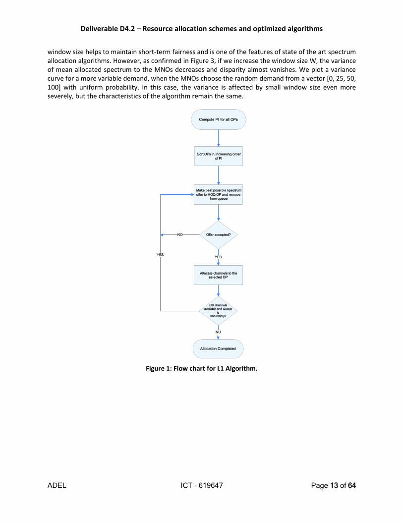
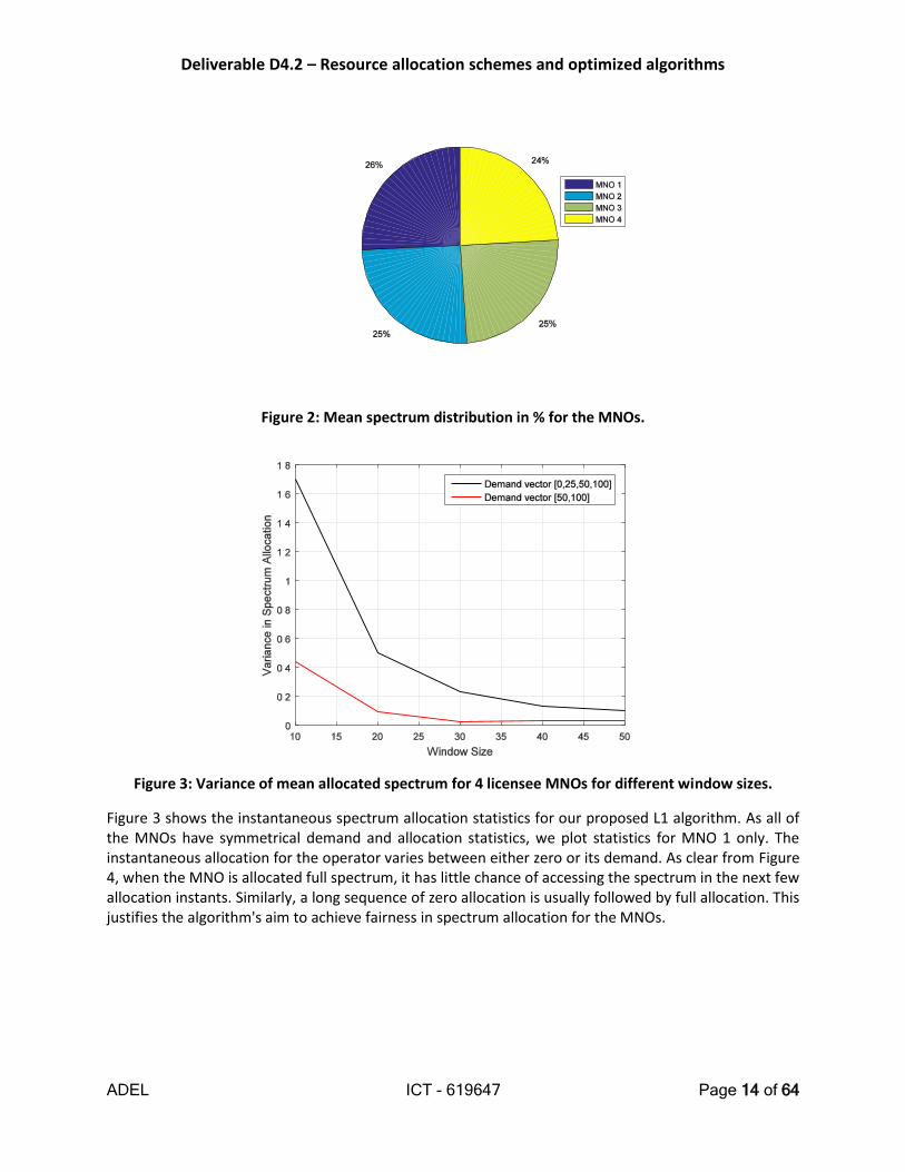
The flow chart for the L1 algorithm is shown in Figure 1. We use Monte Carlo simulations to evaluate the performance of the proposed algorithm. The window size W for computing PI is set to 20 to ensure more short term fairness. As PI computation for each MNO requires spectrum allocation in last W instants, we initialize simulations by having W time slots with zero spectrum allocation and random PI (between 0 and 1) values for every MNO. In the simulations, we consider N=4 and incumbent spectrum B is normalized to 100 units without loss of generality. At each spectrum allocation instant, every MNO n chooses the demand randomly out of a vector of values [50,100] with uniform probability. We simulate 10,000 spectrum allocation instants to compute mean spectrum allocation for each MNO. Without loss of generality, we assume that an MNO accepts whatever spectrum is offered by the LSA band manager after running L1 algorithm. Figure 2 shows the mean spectrum allocation to 4 MNOs. It is clear that the algorithm is fair in the long term and divides spectrum among the MNOs almost uniformly. MNO 1 is allocated one percent more spectrum than the mean while MNO 4 is allocated 1% less. However, this disparity in allocation is attributed to small window size W=20 for PI computation. We used small W in our experiments as small
Deliverable D4.2 – Resource allocation schemes and optimized algorithms
ADEL ICT - 619647 Page 13 of 64
window size helps to maintain short-term fairness and is one of the features of state of the art spectrum allocation algorithms. However, as confirmed in Figure 3, if we increase the window size W, the variance of mean allocated spectrum to the MNOs decreases and disparity almost vanishes. We plot a variance curve for a more variable demand, when the MNOs choose the random demand from a vector [0, 25, 50, 100] with uniform probability. In this case, the variance is affected by small window size even more severely, but the characteristics of the algorithm remain the same.
Figure 1: Flow chart for L1 Algorithm.
Deliverable D4.2 – Resource allocation schemes and optimized algorithms
ADEL ICT - 619647 Page 14 of 64
Figure 2: Mean spectrum distribution in % for the MNOs.
Figure 3: Variance of mean allocated spectrum for 4 licensee MNOs for different window sizes.
Figure 3 shows the instantaneous spectrum allocation statistics for our proposed L1 algorithm. As all of the MNOs have symmetrical demand and allocation statistics, we plot statistics for MNO 1 only. The instantaneous allocation for the operator varies between either zero or its demand. As clear from Figure 4, when the MNO is allocated full spectrum, it has little chance of accessing the spectrum in the next few allocation instants. Similarly, a long sequence of zero allocation is usually followed by full allocation. This justifies the algorithm's aim to achieve fairness in spectrum allocation for the MNOs.

Deliverable D4.2 – Resource allocation schemes and optimized algorithms
ADEL ICT - 619647 Page 15 of 64
Figure 4: Performance evaluation for short-term spectrum allocation for MNO 1. The 21-200 spectrum allocation instants are plotted.
To study the convergence of the proposed algorithm, let us define moving average of the allocated spectrum to an MNO in a time slot t by,
�̅�(𝑡) =1
𝑊∑ 𝐵(𝑗)
𝑡
𝑗−𝑡−𝑊+!
It is evident that moving average of the allocated spectrum for MNO 1 converges to its mean after very few iterations and diverges marginally afterwards.
1.2 Spectrum auction resource allocation in small cell/Cloud RAN In this algorithm, cloud-based massive-MIMO antennas and spectrum resources are considered where the antennas cooperate to serve users of multiple virtual network operators (VNOs). Multiple VNOs share the antennas while they utilize orthogonally a pool of shared LSA spectrum resources. The approach in this work uses an auctioning mechanism to achieve the highest possible revenue while meeting minimum rate requirements that VNOs offer to their users.
Deliverable D4.2 – Resource allocation schemes and optimized algorithms
ADEL ICT - 619647 Page 16 of 64
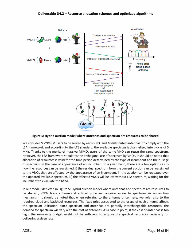
Figure 5: Hybrid auction model where antennas and spectrum are resources to be shared.
We consider N VNOs, K users to be served by each VNO, and M distributed antennas. To comply with the LSA framework and according to the LTE standard, the available spectrum is channelised into blocks of 5 MHz. Thanks to the merits of massive MIMO, users of the same VNO can reuse the same spectrum. However, the LSA framework stipulates the orthogonal use of spectrum by VNOs. It should be noted that allocation of resources is valid for the time period determined by the type of incumbent and their usage of spectrum. In the case of appearance of an incumbent in a given band, there are a few options as to how the resources can be reassigned: i) the residual spectrum from the current auction can be reassigned to the VNOs that are affected by the appearance of an incumbent, ii) the auction can be repeated over the updated available spectrum, iii) the affected VNOs will be left without LSA spectrum, waiting for the incumbent to evacuate the band.
In our model, depicted in Figure 5: Hybrid auction model where antennas and spectrum are resources to be shared., VNOs lease antennas at a fixed price and acquire access to spectrum via an auction mechanism. It should be noted that when referring to the antenna price, here, we refer also to the required cloud and backhaul resources. The fixed price associated to the usage of each antenna affects the spectrum utilisation. Since spectrum and antennas are partially interchangeable resources, the demand for spectrum will vary with the cost of antennas. As a case in point, if the cost of antennas is too high, the remaining budget might not be sufficient to acquire the spectral resources necessary for delivering a given rate.

Deliverable D4.2 – Resource allocation schemes and optimized algorithms
ADEL ICT - 619647 Page 17 of 64
Here, we have adopted a clock auction for the assignment of resources to the VNOs. The clock auction operates in two phases - namely, the price discovery (clock) phase and the final assignment phase. The price of spectrum monotonically increases in each round and VNOs indicate the packages of spectrum and antennas they are willing to buy at a given price. In particular, if the auctioneer detects excess demand for the spectrum after a round of bidding has closed, it increases the posted spectrum price and opens another round of bidding. In our model, in each round each VNO can XOR 2 package bids. A VNO computes the first package bid as the number of antennas and 5 MHz blocks that minimise its cost within its budget constraint, whilst providing its users a minimum rate. The cost is a linear combination of the number of antennas and bandwidth at the prices indicated by the auctioneer. With the exception of spectrum channelisation, this is the same model discussed in [1]. However, since the price of spectrum increases at each round, we also consider a second bidding strategy, which models a less aggressive competitive bidding for the spectrum resources. In order to calculate the second package bid, each VNO starts from the first set of number of antennas and spectrum requirement, and attempts to minimise the bandwidth requirements by incrementing the number of antennas, provided that the minimum rate requirement is satisfied. Then each VNO checks if the cost is less than or equal to its available budget and submits a package bid to the auctioneer. This procedure is shown in Algorithm~\ref{alg:Bid2} where 𝑎𝑖𝑗 ∈ {K, K +
1, … M} and 𝑏𝑖𝑗 ∈ {5,10, … , 𝐵} are the number of antennas and spectrum blocks of width 5 MHz that
VNO i submits to the auctioneer at bid package j, aMax is the maximum number of available antennas, RateMin;I is the minimum required rate for the i-th VNO, and βi is the budget for VNO i.
The clock phase of the auction ends when all excess demand is removed from the market. In the ideal situation, both supply and demand completely match. However, this is unlikely to happen in complex multi-item-unit, multi-item-type auctions. Consequently, the approach that is used in this part of the auction may result in the oversupply of spectrum. This will happen if the bidders private valuation of the minimum required rate is lower than the corresponding cost to acquire spectrum and antennas at the requested price. If this situation arises, the bids are assigned using a revenue maximising approach, i.e. using a winner determination algorithm. This algorithm determines which combination of the bids that stood at the last clock price which caused excess demand will maximise the auctioneer's revenue. The winner determination problem can be formulated as follows.

Deliverable D4.2 – Resource allocation schemes and optimized algorithms
ADEL ICT - 619647 Page 18 of 64
where 𝑦𝑖𝑗 = 1if package 𝑗 of bidder 𝑖 is accepted, otherwise 𝑦𝑖𝑗 = 0. 𝑐𝑎 and 𝑐𝑏 are the costs per antenna
and spectrum block, respectively. Finally, 𝐵is the total available bandwidth.
1.2.1.1 Key Results
The simulated scenario is based on the auctioning strategy explained earlier. The scenario includes 15 VNOs competing in a bid to acquire spectrum and infrastructure to meet their requested minimum rate. The minimum requested rate is the same for all the operators. We consider 10 users per VNO that are randomly distributed in a given area. A total of 64 antennas are available for sharing between the VNOs. The total available spectrum is 50 MHz, where each VNO can acquire spectrum in blocks of 5 MHz, according to the LSA rules. The budget of each operator is proportional to the rate required by its users. The results of the simulated scenario are depicted in Figure 6 and 7. Figure 6 depicts the number of required antennas, again as a function of the minimum rate and antenna price. Figure 7 illustrates two directly related aspects - the required bandwidth and number of VNOs that can be served. To understand the trends, these figures should be considered together. Looking along the x-axis in both figures, we can see that for the lowest considered user rate, the same number of antennas and spectrum are required, regardless of the antenna price. In this case, spectrum is abundant as VNOs cannot lease less than 5 MHz of spectrum, or less than 10 antennas. This spectrum is therefore sufficient to provide the required rate, with the minimum number of antennas. In total, 10 VNOs are served. As the minimum considered user rate increases (looking along the y-axis), the number of antennas increases up to the highest possible number. The VNOs can still serve its users with 5 MHz of spectrum, but with the increasing number of antennas. This is the case until maximum number of antennas is reached and as long as the antenna price is less than a certain value (approximately 250 % of the budget per kbps). For higher antenna prices, it is more cost-effective for VNOs to buy more spectrum than to further increase the number of antennas. The spectrum requirement therefore jumps to the region of 10 MHz, when 5 VNOs can be served. This trends repeats itself with 10 and 15 MHz of spectrum, serving 5 and 3 VNOs, respectively. It should be noted that this periodicity with the number of antennas is observed only in the case when discrete spectrum is considered, which is one of the main differences between this and the case when continuous spectrum is considered.

Deliverable D4.2 – Resource allocation schemes and optimized algorithms
ADEL ICT - 619647 Page 19 of 64
Figure 6: Number of antennas assigned to each allocated VNO in correspondence to a particular rate requirement (y-axis) and antenna cost (x-axis). Antenna cost incorporates the required cloud and backhaul resources.
Figure 7: Number of VNOs in correspondence to a particular rate requirement (y-axis) and antenna cost (x-axis). Again, antenna cost incorporates the required cloud and backhaul resources.

Deliverable D4.2 – Resource allocation schemes and optimized algorithms
ADEL ICT - 619647 Page 20 of 64
1.2.1.1.1 Comparison with Fixed Sharing
In this subsection, we compare the results of auction-based sharing with fixed-based allocation of resources. In that, we consider two approaches - one with orthogonal and equal allocation of both spectrum and antennas, and the other with equal allocation of spectrum, where all VNOs can utilise all the antennas. Figure 8 depicts the number of served VNOs versus the rate requirement for the considered approaches. It should be noted that two different antenna price values are evaluated for the auction-based sharing. The case of fixed sharing with equal and orthogonal allocation of spectrum where all the antennas are shared can be considered as a benchmark. Namely, as in our study all VNOs have the same rate requirements, under the assumption of orthogonal spectrum allocation, using all antennas and equally dividing the spectrum among the VNOs is the optimal solution in terms of system efficiency.
The fixed sharing case with orthogonal usage of antennas serves the lowest number of VNOs, regardless of the rate. This degradation in the number of VNOs that can be served is due to the fact that virtualisation is not exploited i.e. each VNO uses smaller number of antennas. As it is shown in Figure 8, the auction-based approach for two different antenna prices under consideration outperform the fixed sharing case with orthogonal utilisation of antennas. Furthermore, with a cost of antennas that is less than approximately 250% of the budget, we can always achieve the optimal performance through the auction-based approach.
Figure 8: Fixed sharing versus auction-based sharing.

Deliverable D4.2 – Resource allocation schemes and optimized algorithms
ADEL ICT - 619647 Page 21 of 64
1.3 Iterative convex approximation algorithm
We propose an iterative algorithm to solve the following general optimization problem:
(1)
where is a closed and convex set, and is a proper and differentiable function
with a continuous gradient. We assume that problem (1) has a solution. We propose an iterative algorithm that solves (1) as a sequence of successively refined approximate problems, each of which is much easier to solve than the original problem (1), e.g., the approximate problem can be decomposed into independent subproblems that even exhibits a closed-form solution.
In iteration t, let be the approximate function of around the point . Then the approximate
problem is
(2)
and its optimal point and solution set is denoted as and , respectively:
(3)
We assume that the approximate function satisfies the following technical conditions:
(A1) The approximate function is pseudo-convex in x for any given ;
(A2) The approximate function is continuously differentiable in x for any given and
continuous in y for any ;
(A3) The gradient of and the gradient of are identical at for any , i.e.,
;
Based on (3), we define the mapping that is used to generate the sequence of points in the proposed algorithm:
Given the mapping , the following properties hold. Proposition 1 [Stationary point and descent direction]
(i) A point y is a stationary point of (1) if and only if defined in (3);
(ii) (ii) If y is not a stationary point of (1), then is a descent direction of :
If is not a stationary point, according to Proposition 1, we define the vector update in the (t+1)-th iteration as:
(4)
where is an appropriate stepsize that can be determined by either the exact line search (also
known as the minimization rule) or the successive line search (also known as the Armijo rule). Since , and , it follows from the convexity of that .
Deliverable D4.2 – Resource allocation schemes and optimized algorithms
ADEL ICT - 619647 Page 22 of 64
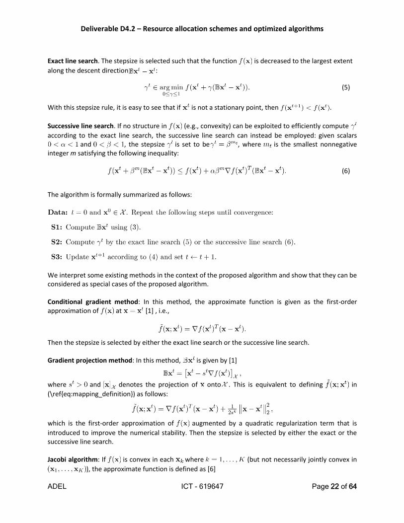
Exact line search. The stepsize is selected such that the function is decreased to the largest extent
along the descent direction :
(5)
With this stepsize rule, it is easy to see that if is not a stationary point, then .
Successive line search. If no structure in (e.g., convexity) can be exploited to efficiently compute
according to the exact line search, the successive line search can instead be employed: given scalars and , the stepsize is set to be , where is the smallest nonnegative
integer m satisfying the following inequality:
(6)
The algorithm is formally summarized as follows:
We interpret some existing methods in the context of the proposed algorithm and show that they can be considered as special cases of the proposed algorithm. Conditional gradient method: In this method, the approximate function is given as the first-order approximation of at [1] , i.e.,
Then the stepsize is selected by either the exact line search or the successive line search. Gradient projection method: In this method, is given by [1]
where and denotes the projection of onto . This is equivalent to defining in
(\ref{eq:mapping_definition}) as follows:
which is the first-order approximation of augmented by a quadratic regularization term that is
introduced to improve the numerical stability. Then the stepsize is selected by either the exact or the successive line search. Jacobi algorithm: If is convex in each where (but not necessarily jointly convex in
), the approximate function is defined as [6]

Deliverable D4.2 – Resource allocation schemes and optimized algorithms
ADEL ICT - 619647 Page 23 of 64
(7)
where for . The k-th component function in (7) is
obtained from the original function by fixing all variables except , i.e., , and further
adding an (optional) quadratic regularization term. Since in (7) is convex, Assumption (A1) is
satisfied. Based on the observations that
we conclude that Assumption (A3) is satisfied by the choice of the approximate function in (7). The resulting approximate problem is given by
(8)
while the stepsizes are then determined by line search. To guarantee the convergence, the condition proposed in [8] is that for all k in (7). However, this may destroy the convenient structure that could otherwise be exploited. In contrast to this, in the case , problem (8) may exhibit a closed-form solution. In the proposed method, the convergence is guaranteed even when in (7) since
in (7) is convex when for all k and it naturally satisfies the pseudo-convexity assumption
specified by Assumption (A1). The structure inside the constraint set , if any, may be exploited to solve (8) even more efficiently. For
example, the constraint set consists of separable constraints in the form of for some
convex functions . Since subproblem (8) is convex, primal and dual decomposition techniques can
readily be used to solve (8) efficiently [5] . In the case that the constraint set has a Cartesian product structure, the subproblem (8) is naturally decomposed into K sub-problems, one for each variable, which are then solved in parallel. This is
commonly known as the Jacobi update: and
(9)
where can be interpreted as variable 's best-response to other variables when
.
An example application of the general formulation (1) is the MIMO Broadcast Channel (BC) capacity computation problem. Consider a MIMO BC where the channel matrix characterizing the transmission from the base station to user is denoted by , the transmit covariance matrix of the signal from the base station to user is denoted as , and the noise at each user is an additive independent and identically distributed Gaussian vector with unit variance on each of its elements. Then the sum capacity of the MIMO BC is [9]
(10)

Deliverable D4.2 – Resource allocation schemes and optimized algorithms
ADEL ICT - 619647 Page 24 of 64
where is the power budget at the base station. Problem (10) is a convex problem whose solution cannot be expressed in closed-form and can only be found iteratively. To apply the proposed algorithm, we invoke (7)-(8) and the approximate problem at the $t$-th iteration is
(11)
where . The approximate function is concave in Q and differentiable in
both Q and , and thus Assumptions (A1)-(A3) are satisfied. Problem (11) is convex and the sum-power constraint coupling is separable, so dual decomposition techniques can be used [Palomar2006]. In particular, the constraint set has a nonempty interior, so strong duality holds and (11) can be solved from the dual domain by relaxing the sum-power constraint into the Lagrangian [3] :
(12)
where and is the optimal Lagrange multiplier that satisfies the following conditions:
, , , and can be found efficiently using the
bisection method . The problem in (12) is uncoupled among different variables in both the objective function and the constraint set, so it can be decomposed into a set of smaller subproblems which are solved in parallel:
and
and exhibits a closed-form expression based on the waterfilling solution [4] . Thus problem (11) also has a closed-form solution up to a Lagrange multiplier that can be found efficiently using the bisection method. With the update direction , the base station can implement the exact line search to determine the stepsize using the bisection method described. We remark that when the channel matrices are rank deficient, problem (11) is convex but not strongly convex, but the proposed algorithm with the approximate problem (11) still converges. However, if the approximate function in [6] is used, an additional quadratic regularization term must be included into (11) (and thus (12)) to make the approximate problem strongly convex, cf. (7), but the resulting approximate problem no longer exhibits a closed-form solution and thus are much more difficult to solve.

Deliverable D4.2 – Resource allocation schemes and optimized algorithms
ADEL ICT - 619647 Page 25 of 64
Simulations. The parameters are set as follows. The number of users is K=20 and K=100, the number of transmit and receive antenna is (5,4), and P=10 dB. The simulation results are averaged over 20 instances.
Figure 9: Sum-rate versus the number of iterations
We apply the proposed algorithm with approximate problem (11) and stepsize based on the exact line search, and compare it with the iterative algorithm proposed in [4] , which uses the same approximate problem (11) but with a fixed stepsize (K is the number of users). It is easy to see from Figure
9 that the proposed method converges very fast (in less than 10 iterations) to the sum capacity, while the method of [4] requires many more iterations. This is due to the benefit of the exact line search applied in our algorithm over the fixed stepsize tends to be overly conservative. Employing the exact line search adds complexity as compared to the simple choice of a fixed stepsize, however, since the objective function of (10) is concave, the exact line search consists in maximizing a differentiable concave function with a scalar variable, and it can be solved efficiently by the bisection method with affordable cost. More specifically, it takes 0.0023 seconds to solve problem (11) and 0.0018 seconds to perform the exact line search. Therefore, the overall CPU time (time per iteration number of iterations) is still dramatically decreased due to the notable reduction in the number of iterations. Besides, in contrast to the method of [4] , increasing the number of users K does not slow down the convergence, so the proposed algorithm is scalable in large networks.

Deliverable D4.2 – Resource allocation schemes and optimized algorithms
ADEL ICT - 619647 Page 26 of 64
Figure 10: error versus the number of iterations
We also compare the proposed algorithm with the iterative algorithm of [7] , which uses the approximate problem (11) but with an additional quadratic regularization term, cf. (7), where for all k, and decreasing stepsizes where d=0.01 is the so-called decreasing rate that controls the
rate of decrease in the stepsize. We can see from Figure 10 that the convergence behavior of [7] is rather sensitive to the decreasing rate d. The choice d=0.01 performs well when the number of transmit and receive antennas is 5 and 4, respectively, but it is no longer a good choice when the number of transmit and receive antenna increases to 10 and 8, respectively. A good decreasing rate d is usually dependent on the problem parameters and no general rule performs equally well for all choices of parameters. We remark once again that the complexity of each iteration of the proposed algorithm is very low because of the existence of a closed-form solution to the approximate problem (11), while the approximate problem proposed in [7] does not exhibit a closed-form solution and can only be solved iteratively. Specifically, it takes CVX (version 2.0) 21.1785 seconds (based on the dual approach (12) where is found by bisection). Therefore, the overall complexity per iteration of the proposed algorithm is much lower than that of [6].

Deliverable D4.2 – Resource allocation schemes and optimized algorithms
ADEL ICT - 619647 Page 27 of 64
1.4 Frequency agile centralized resource allocation algorithm
1.4.1 Objectives
In this section, we intend to describe a simple centralized frequency allocation scheme, developed under Task 4.1, and compare it in a specific ADEL reference scenario with a distributed algorithm, proposed under the Task 4.2 umbrella. We should stress that both algorithms operate at level 1. In ADEL terminology, this means both algorithms allocate frequencies to multiple networks and not to multiple end-users. The comparison in performed in terms of i) the probability of denying LSA licensees’ allocation requests, and ii) the probability of the LSA licensees having to return previously allocated spectrum in case an incumbent reclaims it afterwards. The work carried out, illustrates the benefits brought by the adoption of LSA, as well as the increased performance expected from the centralized algorithm.
1.4.2 Main Activities
One of the key enabling technologies behind LSA is software defined radio (SDR) that brought to the mobile networks the flexibility to be reconfigured when necessary. One of the reconfiguration features with the most importance for LSA is, obviously, related with frequency agility. For that reason, in this section, we intend to propose a simple centralized frequency allocation scheme, developed within task T4.1, which uses the frequency agility capabilities of the LSA licensees. It should be mentioned that, under ADEL terminology, the algorithm operates at level 1. This means it will allocate frequencies to LSA licensees’ networks, and not to end-users.
We consider the band 2300-2400MHz as the LSA band. In many European countries the incumbents in this band are transmissions from PMSE’s wireless cameras, using e.g. DVB-T and 10MHz channelization.
In ADEL we consider one of the most likely LSA licensees using the band will be mobile operators using the band to provide mobile broadband services. Therefore, in the algorithms being described, we consider these operators are willing to use LTE and also 10MHz channelization.
Having said that, in short, the problem consists in dynamically allocate C=10 channels, each with a 10MHz bandwidth, to N1 incumbents and N2 LSA licensees whose service areas overlap in space.
We consider N1≤C as it is unlikely that the national regulators assign the same channel to many PMSE incumbent network in the same spot at the same time. As LSA is based on a temporary use of parts of the spectrum, we see as desirable to consider N2 as high as possible, and therefore most likely, we will have situations where N2>C. In our study we assume N1=6 incumbent networks, and N2=12 LSA licensees networks. Figure 11 depicts one example of a possible sharing configuration of the LSA band where only the minimal amount of LSA licensees (C-N1) is authorized to use the band, while there are (N2-C+N1) LSA licensees cannot use it.
Figure 11: Example of one of the possible sharing configurations of the LSA band
We assume requests to access the spectrum for a given period, arrive at any instant to the LSA band Manager. The only constraint imposed by LSA is that these requests are made in advance, in relation to the period of interest. When processing the requests, the LSA Band Manager must obey to the following rules:
A B C D E F
f 1 2 3 4
Incumbent Licensee
2.3GHz 2.4GHz

Deliverable D4.2 – Resource allocation schemes and optimized algorithms
ADEL ICT - 619647 Page 28 of 64
As N1≤C, the requests from incumbent networks are always served. If the band is entirely occupied,
an LSA licensee is asked to leave the band, i.e. incumbents can reclaim their spectrum back after it
has already been allocated to an LSA licensee.
The requests from LSA licensees’ networks are only served if there are spectrum still available.
Requests that cannot be served, are dropped.
Spectrum is used in an exclusive way (i.e. only the operator that has been assigned a specific
channel for a specific time and location may use that frequency in that period and location).
The algorithm intends to maximize the contiguous spectrum that remains available, in order to maximize the spectrum utilization efficiency. This would have positive impact in the blocking probability, especially when the LSA licensees are wider in frequency than the incumbents.
Figure 12: Exemplification of the centralized allocation algorithm
This algorithm must be implemented in a centralized way, because the LSA Band Manager must know which incumbents and which LSA licensees are occupying each channel in order to be able to give the commands to switch frequency to the correct network.
1.4.3 Key Results
We determined the performance of this centralized algorithm in terms of i) the probability of denying LSA licensees’ allocation requests, and ii) the probability of the LSA licensees having to return previously allocated spectrum in result of an incumbent reclaims it.
As we do not have real data concerning the spectrum utilization of incumbents and licensees, we assumed that, for both types of networks, the number of arrivals of allocation requests may be modelled by a Poisson random process with rate λ, while the allocation period is modeled by a negative exponential distribution with mean time 1/µ.
The scenario under study considers C=10 channels, N1=6 incumbents and N2=12 LSA licensees. We considered all incumbents have similar behavior, and that each of them use the spectrum, on average, during one hour, i.e 1/µ1=1 hour. In a similar way, we considered all the licensees operate in a similar way, and they use the spectrum on average 12 minutes, i.e. 1/µ2= 1/5 hour.
5
A 1 B C 2 D 3 4 5 6
Licensee 7 appears when band is full -> Request blocked Incumbent E appears -> Licensee 6 is dropped
A 1 E C 2 D 4 3 Licensee 2 goes away -> Licensee 5 occupies its place
Incumbent A goes away -> Licensee 4 occupies its place
A 1 E C 5 D 4 3
4 1 E C 5 D 3
A 1 B C 2 D 4 3 5 E
Incumbent B goes away -> Incumbent E occupies its place
time
frequency
Deliverable D4.2 – Resource allocation schemes and optimized algorithms
ADEL ICT - 619647 Page 29 of 64
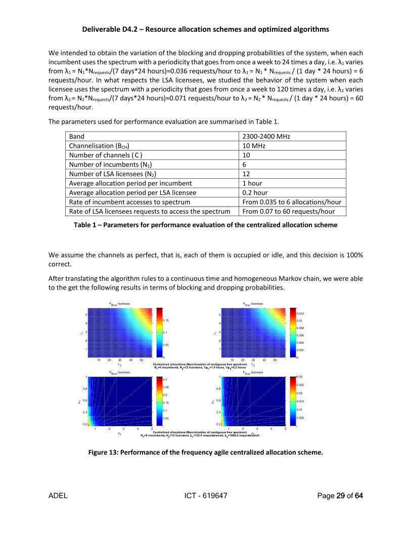
We intended to obtain the variation of the blocking and dropping probabilities of the system, when each incumbent uses the spectrum with a periodicity that goes from once a week to 24 times a day, i.e. λ1 varies from λ1 = N1*Nrequests/(7 days*24 hours)≈0.036 requests/hour to λ1 = N1 * Nrequests / (1 day * 24 hours) = 6 requests/hour. In what respects the LSA licensees, we studied the behavior of the system when each licensee uses the spectrum with a periodicity that goes from once a week to 120 times a day, i.e. λ2 varies from λ2 = N2*Nrequests/(7 days*24 hours)≈0.071 requests/hour to λ2 = N2 * Nrequests / (1 day * 24 hours) = 60 requests/hour.
The parameters used for performance evaluation are summarised in Table 1.
Band 2300-2400 MHz
Channelisation (BCH) 10 MHz
Number of channels ( C ) 10
Number of incumbents (N1) 6
Number of LSA licensees (N2) 12
Average allocation period per incumbent 1 hour
Average allocation period per LSA licensee 0.2 hour
Rate of incumbent accesses to spectrum From 0.035 to 6 allocations/hour
Rate of LSA licensees requests to access the spectrum From 0.07 to 60 requests/hour
Table 1 – Parameters for performance evaluation of the centralized allocation scheme
We assume the channels as perfect, that is, each of them is occupied or idle, and this decision is 100% correct.
After translating the algorithm rules to a continuous time and homogeneous Markov chain, we were able to the get the following results in terms of blocking and dropping probabilities.
Figure 13: Performance of the frequency agile centralized allocation scheme.
1
2
3
4
5
10 20 30 40 50
2
PBlock
licensees
1
0
0.05
0.1
0.15
1
2
3
4
5
10 20 30 40 50
2
PDrop
licensees
1
0
0.002
0.004
0.006
0.008
0.01
0.012
0.2
0.4
0.6
0.8
1
1 2 3 4 5
2
PBlock
licensees
1
0.05
0.1
0.15
0.2
0.25
0.3
0.2
0.4
0.6
0.8
1
1 2 3 4 5
2
PDrop
licensees
1
0.005
0.01
0.015
0.02
0.025
0.03
Centralized allocations (Maximization of contiguous free spectrum)N
1=6 incumbents, N
2=12 licensees, 1/
1=1.0 hours, 1/
2=0.2 hours
Centralized allocations (Maximization of contiguous free spectrum)N
1=6 incumbents, N
2=12 licensees,
1=132.0 requests/week,
2=1608.0 requests/week
Deliverable D4.2 – Resource allocation schemes and optimized algorithms
ADEL ICT - 619647 Page 30 of 64
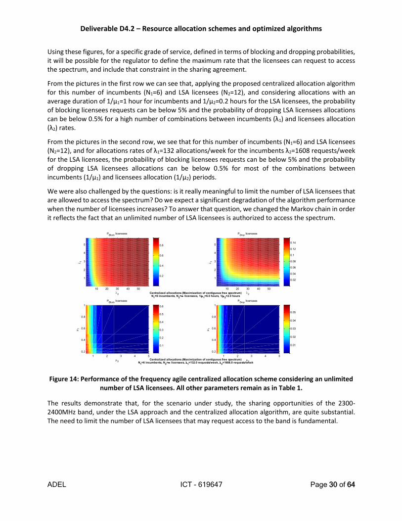
Using these figures, for a specific grade of service, defined in terms of blocking and dropping probabilities, it will be possible for the regulator to define the maximum rate that the licensees can request to access the spectrum, and include that constraint in the sharing agreement.
From the pictures in the first row we can see that, applying the proposed centralized allocation algorithm for this number of incumbents (N1=6) and LSA licensees (N2=12), and considering allocations with an average duration of 1/µ1=1 hour for incumbents and 1/µ2=0.2 hours for the LSA licensees, the probability of blocking licensees requests can be below 5% and the probability of dropping LSA licensees allocations can be below 0.5% for a high number of combinations between incumbents (λ1) and licensees allocation (λ2) rates.
From the pictures in the second row, we see that for this number of incumbents (N1=6) and LSA licensees (N2=12), and for allocations rates of λ1=132 allocations/week for the incumbents λ2=1608 requests/week for the LSA licensees, the probability of blocking licensees requests can be below 5% and the probability of dropping LSA licensees allocations can be below 0.5% for most of the combinations between incumbents (1/µ1) and licensees allocation (1/µ2) periods.
We were also challenged by the questions: is it really meaningful to limit the number of LSA licensees that are allowed to access the spectrum? Do we expect a significant degradation of the algorithm performance when the number of licensees increases? To answer that question, we changed the Markov chain in order it reflects the fact that an unlimited number of LSA licensees is authorized to access the spectrum.
Figure 14: Performance of the frequency agile centralized allocation scheme considering an unlimited number of LSA licensees. All other parameters remain as in Table 1.
The results demonstrate that, for the scenario under study, the sharing opportunities of the 2300-2400MHz band, under the LSA approach and the centralized allocation algorithm, are quite substantial. The need to limit the number of LSA licensees that may request access to the band is fundamental.
1
2
3
4
5
10 20 30 40 50
2
PBlock
licensees
1
0.2
0.4
0.6
0.8
1
2
3
4
5
10 20 30 40 50
2
PDrop
licensees
1
0.02
0.04
0.06
0.08
0.1
0.12
0.14
0.2
0.4
0.6
0.8
1
1 2 3 4 5
2
PBlock
licensees
1
0.1
0.2
0.3
0.4
0.5
0.6
0.2
0.4
0.6
0.8
1
1 2 3 4 5
2
PDrop
licensees
1
0.01
0.02
0.03
0.04
0.05
Centralized allocations (Maximization of contiguous free spectrum)N
1=6 incumbents, N
2= licensees, 1/
1=6.0 hours, 1/
2=2.0 hours
Centralized allocations (Maximization of contiguous free spectrum)N
1=6 incumbents, N
2= licensees,
1=132.0 requests/week,
2=1608.0 requests/week

Deliverable D4.2 – Resource allocation schemes and optimized algorithms
ADEL ICT - 619647 Page 31 of 64
1.5 Fair Opportunistic scheduler for real time traffic with reduced feedback size
We consider the small cells scenario where different eNBs share one or multiple LSA channels under the control of a central macro base station (BS), (Figure 15).
Macro BS
Small Cell Small
Cell
Small Cell
Small Cell
Small Cell
Small Cell
Small Cell
Small Cell
Figure 15: LSA centrally controlled small cell scenario
The feedback from the different eNBs to the BS is supposed to be fast enough, yet limited, to allow scheduling of end users (UEs) attached to the eNBs on the LSA channels to be performed by the BS.
Opportunistic scheduling algorithms are known to achieve good performance in term of achieved throughput for best effort traffics (delay unlimited) by exploiting the multiuser diversity. Indeed, for delay tolerant traffics, it has been shown that scheduling at each slot the user undergoing the best radio conditions in fading environment maximizes the overall system throughput in the saturated regime, this is known as the multiuser diversity scheduling (MUDS) [10] . Multiuser diversity comes from the fact that in a wireless communication system, the fading channels between the base station and each user undergo independent variations, and then it is more likely to always find a user with channel in good radio state. However, the maximization of throughput in MUDS comes at the expense of poor fairness in the offered throughput as strong users are more served than weaker ones.
The proportional fair scheduling (PFS) algorithm has been introduced as an attractive solution to the problem since it provides a good compromise between throughput maximization and service fairness [11] . The idea behind PFS is to ensure more fairness to the scheduling by normalizing the instantaneous achievable radio rate by the past average throughput in the cost function of each user. The algorithm is widely used in current cellular systems and also exhibits low implementation complexity which increases its attractiveness, and tends to achieve perfect temporal fairness as the network size increases.
Scheduling algorithms based on the cumulative distribution function of users' rates have been introduced

Deliverable D4.2 – Resource allocation schemes and optimized algorithms
ADEL ICT - 619647 Page 32 of 64
in [12] to better benefit from multiuser diversity while offering perfect temporal fairness even for reduced number of users. Unlike PFS, in cumulative distribution function fair scheduling, the decision is based on the knowledge of the CDF of users' rates in order to grant channel access to users when they are near their own peaks. These algorithms exhibit good performance in terms of throughput and fairness, their main drawback however is their requirement to have knowledge of the CDF of the users' rates.
Most of studies on scheduling algorithms consider the saturated regime case in order to measure the performance limits of these algorithms. In real scenarios however, saturated regimes appear only in extreme and temporary situations regarding the quasi-systematic presence of admission control mechanisms that prevent them. The queue maximum proportional fair scheduling (QMPFS) algorithm has been introduced in [13] to exploit multiuser diversity in terms of both radio condition and traffic characteristics. The main idea of this algorithm is to schedule a user when it experiences radio condition near the maximum observed over a window time and when its buffer occupation is near the maximum observed over a window time.
In this work, we consider opportunistic scheduling of heterogeneous real time traffic. As for fairness constraint, delay constraint will reduce the achieved throughput, as the scheduler will have to exploit the multiuser diversity observed only within the delay limit.
The best known scheduler for delay constrained traffic is the Modified Largest Weighted Delay First (M-LWDF) algorithm [14] . It relies however on the delay information of each packet, which is not feasible in practical system where the feedback size is limited. We introduce the delay constrained maximum proportional fair scheduler (DC-MPFS), a modified version of the QMPFS algorithms that relies only on reduced information on the delay. The performance of the new algorithm is compared to those of the PFS and the MLWDF ones.
1.5.1 Setting
We consider a wireless communication system consisting in one base station controlling 𝐾 eNBs. We without loss of generality, we suppose that each eNB is communicating with 1 users over a block fading channel of width 𝑊 in a time-slotted manner (time division multiple access). We assume that the channel gains are independent but not necessarily identically distributed across the users. We further assume that the channel gains remain constant during each slot but change from one slot to another, and we assume that the scheduler has perfect information of the fading processes of each user. Let ℎ𝑘,𝑛 denotes the
channel state of user 𝑘 (attached to eNB 𝑘) at slot 𝑛 and 𝑟𝑘,𝑛 = 𝑙𝑜𝑔2(1 + 𝛽𝑃ℎ𝑘,𝑛
𝑁0) the system rate if user
𝑤 is scheduled at slot 𝑛, where 𝑃 is the transmit power, 𝑁0 the thermal noise power, and 0 < 𝛽 < 1 the SNR gap between the considered transmission system and its Shannon capacity limit.
In case where ℎ𝑘 are Rayleigh distributed with parameter 𝜎𝑘, the probability density function (PDF) of ℎ𝑘 is given as
𝑃(ℎ𝑘 = 𝑥) =1
𝜎𝑘𝑒
−𝑥
𝜎𝑘
We consider homogeneous real time traffic where packets arrive independently at each user's queue according to a discrete time Markov process of intensity ‘𝜆’ and each packet's length is exponentially distributed with mean ‘ 𝜇 ’. Delay constraints on each user traffic are however heterogeneous and expressed as
𝑃(𝐷𝑘 > 𝐷𝑚𝑎𝑥𝑘) ≤ 𝜀

Deliverable D4.2 – Resource allocation schemes and optimized algorithms
ADEL ICT - 619647 Page 33 of 64
Where 𝐷𝑘 is the delay experienced by user 𝑘 and 𝐷𝑚𝑎𝑥𝑘 is the de maximum delay tolerated by user 𝑘.
1.5.2 Opportunistic schedulers
1.5.2.1 Proportional Fair Scheduler
The Proportional Fair Scheduling was aims to take advantage of multiuser diversity while providing good fairness level of channel access among users. The idea behind it is to normalize the score function of each user, i.e. user rate, by its average. Hence, the scheme selects to schedule the user who is experiencing the best fading realization compared to its own past conditions, and not the user with the absolute best instantaneous rate.
The algorithm works as follows:
𝑤 = 𝑎𝑟𝑔𝑚𝑎𝑥𝑘=1,.,𝐾 𝑟𝑘,𝑛
𝑅𝑘,𝑛
𝑊ℎ𝑒𝑟𝑒 𝑅𝑘,𝑛 = {(1 −
1
𝑇𝑐) 𝑅𝑘,𝑛−1 +
1
𝑇𝑐𝑟𝑘,𝑛 𝑖𝑓 𝑘 𝑖𝑠 𝑠𝑐ℎ𝑒𝑑𝑢𝑙𝑒𝑑
(1 −1
𝑇𝑐) 𝑅𝑘,𝑛−1 𝑜𝑡ℎ𝑒𝑟𝑤𝑖𝑠𝑒
‘Tc’ (Tc >1) is the length of the moving average window. The PFS algorithm is not suited for real time traffics as it doesn’t take into account the delay in its scheduling decision
1.5.2.2 Modified Largest Weighted Delay First Scheduler
The M-LWDF algorithm uses both the delay and the channel information to make its scheduling decision. The algorithm works as follows:
𝑤 = 𝑎𝑟𝑔𝑚𝑎𝑥𝑘=1,.,𝐾 − log (𝜀
𝐷𝑚𝑎𝑥𝑘)
𝑟𝑘,𝑛
𝐸[𝑟𝑘,𝑛]𝐷𝑘,𝑛
Where 𝐷𝑘,𝑛 is the delay of the head-of-line packet of user 𝑘at slot 𝑛.
The role of the ′log′ term is to differentiate the users depending on their QoS constraint.
1.5.2.3 Delay Constrained Maximum Proportional Fair Scheduler
In order to reduce the feedback information size, we introduce the DC-MPFS which is a modification of the QMPFS algorithm that take into account the delay constraints.
The algorithm works as follows:
𝑤 = 𝑎𝑟𝑔𝑚𝑎𝑥𝑘=1,.,𝐾
𝑟𝑘,𝑛
𝑅𝑚𝑎𝑥𝑘,𝑛𝑁𝐷𝑘,𝑛
Where 𝑅𝑚𝑎𝑥𝑘,𝑛 = 𝑎𝑟𝑔𝑚𝑎𝑥𝑚=0…𝑀−1 𝑟𝑘,𝑛−𝑚

Deliverable D4.2 – Resource allocation schemes and optimized algorithms
ADEL ICT - 619647 Page 34 of 64
𝑁𝐷𝑘,𝑛 =∑ 𝑆𝑘,𝑛
𝑖 𝐷𝑘,𝑛𝑖
𝑖
𝐷𝑚𝑎𝑥𝑘 ∑ 𝑆𝑘,𝑛𝑖
𝑖
‘𝑅𝑚𝑎𝑥𝑘,𝑛’ is a dynamic threshold value around which the user's channel is considered as in its peak region.
𝑁𝐷𝑘,𝑛 is a weighted average of the delay distance to the maximum delay of the user 𝑘 packets at slot 𝑛.
1.5.3 Simulation results
For our simulation we consider that users are divided in two groups, K/2 weak users have their Rayleigh fading factor ‘𝜎𝑘’ equally separated in the interval [0.05 1] and K/2 strong users in the interval [2 4]. We consider ‘𝛽=1’ and SNR=0dB.
We consider homogenous network traffic (heterogeneity of radio conditions and QoS constraint is sufficient to differentiate users) where packets arrive independently at each user's queue according to a discrete time Markov process of intensity ‘𝜆 = 1’ and each packet's length is exponentially distributed with mean ‘𝜇=1’.
We define the normalized traffic bandwidth (NTB) ‘Wn’ as
𝑊𝑛 =𝑊
∑𝐴𝑘̅̅̅̅
𝑟�̅�
𝐾𝑘=1
where 𝐴𝑘̅̅̅̅ ’ and 𝑟�̅� are respectively the mean arrival rate and the mean radio channel rate of user 𝑘. NTB
is indeed the ratio of the available bandwidth over an upper bound on the bandwidth required to serve the traffic of all users. The upper bound is calculated as if each user is alone in the network and served separately from the others, so there is no scheduling and hence no multiuser diversity gain.
QoS constraints are heterogeneous, the maximum delays of users are random permutations of the set {10, 10+1/(K-1), 10+2/(K-1),…,20} .
We vary the NTB between 0.6 and 1 and we plot in Figure 16 the performance of the 3 schedulers vs. NTB for 𝐾 = 30 and 𝜀 = 10−4. The performance is expressed in term of the number of users for which the QoS constraint is satisfied.
Figure 16: QoS satisfaction Vs. Normalized traffic bandwidth

Deliverable D4.2 – Resource allocation schemes and optimized algorithms
ADEL ICT - 619647 Page 35 of 64
We observe then that the performance of our reduced feedback scheduler CD-MPFS approaches the performance of the M-LWDF scheduler and succeed to satisfies all users with NTB=0.95, which mean that it was able to exploit the multiuser diversity within the delay constraints.
1.6 Opportunistic beamforming for secondary users in Licensed Shared Access networks
In this section we consider that a Licensee system (LS) employing an opportunistic beamforming technique with user scheduling coexists with an Incumbent system (IS). The proposed technique exploits the availability of IS information to LS offered by LSA, to serve the preferred LS user subject to the quality of service of the preferred IS user. In particular, for each generated beam per time slot, the multi-antenna LS base station decides whether to send data to the LS user with the maximum time-averaged rate request, depending on the quality of service requirement of the preferred IS user available in the LSA repository. Simulation performance results for a cellular channel model have shown that the proposed technique is capable of boosting the performance of the overall network.
Multi-antenna techniques play an important role in current mobile broadband systems [23] since they are capable of considerably increasing the capacity of wireless links and improving their reliability. Opportunistic beamforming (OBF) [24] has been proposed as a low feedback technique for the downlink of cellular systems with multi-antenna base stations (BSs). It exploits the inherent multi-user diversity of cellular systems to schedule the mobile user with the most favourable instantaneous channel quality. This technique was later tied up with the waiting times of the active mobile users to reduce the probability of excessive packet delay and improve cell throughput [25] .
In this Section, we present a joint OBF and scheduling technique for the downlink of a secondary (Licensee) wireless system that coexists with a primary (Incumbent) one under the ADEL architectural setup. In particular, both Incumbent and Licensee BSs are equipped with multiple antennas and wish to communicate with a single-antenna IS user and a single-antenna LS user, respectively. Each BS is assumed to utilise, in common control phases, a beam chosen in a pseudo-random way from a fixed predetermined set of beams in order to collect the instantaneous signal-to-interference-plus-noise ratios (SINRs) of its mobile users. In every transmission phase, the primary BS schedules its preferred IS users whereas, the secondary BS serves its preferred LS users only when this potential transmission does not degrade the channel quality of the IS below a certain level. To accomplish this, both BSs are assumed to be perfectly synchronised and the secondary BS is assumed to obtain the PU’s QoS requirement instantaneously from the LSA repository. Computer simulation results have shown that the proposed technique exploits multi-user diversity to boost the sum-rate performance of the coexisting systems, especially for large numbers of mobile users.
1.6.1 System and channel model
A primary and a secondary multi-antenna BSs are assumed to coexist under a LSA framework and both wish to communicate with their respective single-antenna mobile users. In particular, the 𝑁𝑝-antenna
primary BS adopts OBF with proportional fair scheduling (PF) [24] to schedule the IS user with the maximum time-averaged rate request. The 𝑁𝑠-antenna secondary BS is assumed perfectly synchronised with the primary BS and utilises OBF with PF only when this operation does not degrade the channel quality of IS user below a certain threshold. Different sets of pseudo-random beams are used by both BSs and for the selected couple of beams per time slot, all IS and LS users report their instantaneous SINRs back to their corresponding BS during a common control phase. If the channel quality of the preferred IS user satisfies a certain level, both BSs are active in the common transmission phase, otherwise, the

Deliverable D4.2 – Resource allocation schemes and optimized algorithms
ADEL ICT - 619647 Page 36 of 64
secondary BS is not allowed to transmit data to its preferred user. This information is assumed to be instantaneously available to the LSA repository and to the secondary BS in order for the latter to send or not data to the preferred user.
Let h𝑘,1 ∈ ℂ1×𝑁𝑝 and h𝑘,2 ∈ ℂ1×𝑁𝑠, with 𝑘 = 1,2, … , 2𝐾 and ℂ representing the complex number set, denote the channel gain vectors between the 𝑘-th mobile user and the primary and secondary BSs, respectively. A block fading channel model is assumed where h𝑘,𝑙 ’s, with 𝑙 = 1 (primary BS) and 2 (secondary BS), remain constant over time slots of length 𝑇 samples. When both BSs send data to their respective users, the baseband time-slotted received signal at the 𝑘 -th user can be mathematically expressed as
𝑦𝑘(𝑡) = ∑ √𝑃𝑙𝒉𝑘,𝑙(𝑡)𝑥𝑙(𝑡) + 𝑛𝑘(𝑡)
2
𝑙=1
(13)
where 𝑥1(𝑡) ∈ ℂ𝑁𝑝×𝑇 and 𝑥2(𝑡) ∈ ℂ𝑁𝑠×𝑇 are matrices with 𝑇 transmitted symbols in time slot 𝑡 from the primary and secondary BS, respectively. Primary BS transmits each symbol with power 𝑃1 and secondary BS with power 𝑃2. In addition, 𝑛𝑘 ∈ ℂ1×𝑇 in (12) denotes the zero-mean additive white Gaussian noise
vector with covariance matrix 𝜎𝑘2𝑰𝑇, where 𝑰𝑇 is the 𝑇 × 𝑇 identity matrix. For cases where the secondary
BS is not allowed to transmit data, the received signal at the 𝑘-th PU is obtained from (13) by setting 𝑃2 =0 . The elements of each 𝒉𝑘,𝑙 are assumed to be independent zero-mean complex normal random
variables (RVs) with variance 𝛼𝑘,𝑙2 given by [26] , eq. (5,5)]
𝛼𝑘,𝑙2 = 𝛽 (
𝑑𝑘,𝑙
𝑑𝑟𝑒𝑓)
−Γ
𝑠𝑘,𝑙𝑔𝑘,𝑙 (14)
In (14), 𝛽 is the median of the path gain at a reference distance 𝑑𝑟𝑒𝑓 with respect to which the path-loss
is measured, 𝑑𝑘,𝑙 is the distance between the 𝑘-th mobile user and the 𝑙-th BS and Γ is the path-loss
exponent such that Γ = 2 for 30m ≤ 𝑑𝑘,𝑙 ≤ 100m and Γ = 3.7 otherwise. Moreover, 𝑠𝑘,𝑙 = 10𝑆/10 is a
log-normal RV with 𝑆 being a zero-mean normal RV with variance 82, and 𝑔𝑘,𝑙 is the normalised direction-based antenna response of the 𝑙-th BS. For example, for the parabolic response model [27] 𝑔𝑘,𝑙 in dB is
given by
𝑔𝑘,𝑙(𝜃𝑘,𝑙 − 𝜔𝑙) = max {−12 (𝜃𝑘,𝑙 − 𝜔𝑙
𝛩)
2
, 𝐴𝑠} (15)
where 𝜃𝑘,𝑙 is the direction of the 𝑘-th user with respect to the location of the 𝑙-th BS, 𝜔𝑙 is the beam direction of the 𝑙-th BS, Θ is the 3 dB beamwidth of the response, and 𝐴𝑠 < 0 is the sidelobe level of the response measured in dB.
1.6.2 Joint OBF and scheduling for LSA networks
During each common control phase of each time slot 𝑡, both primary and secondary BSs transmit their own pilot signal from each of their multiple antennas. The beamforming of pilot signals is chosen for every BS in a pseudo-random way from a fixed predefined set of beams and a BS’s beamforming is assumed to be unknown to the other BS. Then, each mobile user is assumed to perfectly estimate the channel coefficients h𝑘,𝑙 and feed back to its corresponding BS through an error-free link the maximum rate at which it is capable of receiving data during the transmission phase of time slot 𝑡. The maximum requested

Deliverable D4.2 – Resource allocation schemes and optimized algorithms
ADEL ICT - 619647 Page 37 of 64
data rate of the 𝑘-th mobile user, with 𝑘 = 1, 2, . . . , 2𝐾, at the time slot 𝑡 is derived from the Shannon’s capacity formula:
𝑅𝑘(𝑡) = log2[1 + 𝛾𝑘(𝑡)] (16)
where 𝛾𝑘(𝑡) denotes the estimated SINR at the 𝑘-th user at time slot 𝑡. By using (13), the SINR at the 𝑛-th PU, with 𝑛 = 1, 2, . . . , 𝐾, at time slot 𝑡, needed in (16) for the computation of the maximum requested data rate of the 𝑛-th IS user, is obtained as
𝛾𝑛𝐼𝑆(𝑡) =
𝑃1‖h𝑛,1(𝑡)‖2
𝑃2‖h𝑛,2(𝑡)‖2
+ 𝜎𝑛2
(17)
and similarly, the SINR at the 𝑛-th LS user at time slot 𝑡 as
𝛾𝑛𝐿𝑆(𝑡) =
𝑃2‖h𝑛,2(𝑡)‖2
𝑃1‖h𝑛,1(𝑡)‖2
+ 𝜎𝑛2
(18)
According to the single-cell OBF technique with PF [24] , at each time slot 𝑡 the BS schedules the mobile user 𝑘𝑠 with the largest ratio 𝑅𝑘(𝑡)/𝑇𝑘(𝑡), where 𝑇𝑘(𝑡) is the weighted average throughput of the 𝑘-th user at the beginning of time slot 𝑡. This requires that the BS scheduler keeps track of the average throughputs of all its active users and updates them at every time slot using the following formula
𝑇𝑘(𝑡 + 1) = {(1 −
1
𝑊) 𝑇𝑘(𝑡) +
𝑅𝑘(𝑡)
𝑊, 𝑘 = 𝑘𝑠
(1 −1
𝑊) 𝑇𝑘(𝑡), 𝑘 ≠ 𝑘𝑠
(19)
In (19), parameter 𝑊 determines the effective memory of the throughput averaging window and is tied to the latency time scale of the QoS requirement of the network.
1.6.2.1 OBF with PF for LSA LSs
After the control phase of time slot 𝑡 , depending on the fulfillment of the QoS requirement of the preferred IS user 𝑛𝑠 , the secondary BS proceeds to data transmission or remains idle. The QoS requirement to be met is represented by a SINR threshold 𝛾𝑡ℎ(𝑡) and the information related to threshold violation is assumed to become instantaneously available in the LSA repository and hence, to the secondary BS. In particular, among the 𝐾 active IS users, the IS user 𝑛𝑠 at time slot 𝑡 is obtained as
𝑛𝑠 : max𝑛=1,2,…,𝐾
𝑇𝑛−1(𝑡) log2[1 + 𝛾𝑛
𝐼𝑆(𝑡)] (20)
where 𝑇𝑛(𝑡) is given by (19) using (16) and (17), and let its SINR be denoted by 𝛾𝑛𝑠𝐼𝑆(𝑡). If 𝛾𝑛𝑠
𝐼𝑆(𝑡) ≥ 𝛾𝑡ℎ(𝑡),
at the transmission phase of the time slot 𝑡 the primary BS will send data to the IS user 𝑛𝑠 and the secondary BS will transmit to its preferred LS user 𝜈𝑠. The latter user is selected from the 𝐾 active SUs as
𝜈𝑠 : max𝑛=1,2,…,𝐾
𝑇𝑛−1(𝑡) log2[1 + 𝛾𝑛
𝐿𝑆(𝑡)] (21)

Deliverable D4.2 – Resource allocation schemes and optimized algorithms
ADEL ICT - 619647 Page 38 of 64
with 𝑇𝑛(𝑡) obtained from (19) using (16) and (18).
For the cases where it holds 𝛾𝑛𝑠𝐼𝑆(𝑡) < 𝛾𝑡ℎ(𝑡) in the control phase at the time slot 𝑡, the secondary BS
decides to remain idle for the transmission phase of the time slot and only the primary BS transmits to the PU 𝑛𝑠 obtained from (20). It is noted, however, that the threshold of the preferred IS user 𝑛𝑠 might still not be met. Since (20) is based on the SINRs of the IS users and in the transmission phase of the time slot 𝑡 the secondary BS will be inactive, an additional control phase can be utilised to search for the preferred PU based on their signal-to-noise ratio (SNR) values. To this end, the preferred IS user 𝑛𝑠 is obtained from (20) by setting 𝑃2 = 0 in (17).
1.6.3 Performance results
In this section, computer simulation results for the performance of the proposed LSA system are presented. The considered performance metrics are:
i) average system throughput 𝑅𝑠; ii) average time 𝑇 that the secondary BS is idle; and, iii) average violations 𝑉 of the threshold (SINR or SNR) of the preferred IS user.
Both versions of LSA presented, namely LSA with one and two control phases, are compared when the number of mobile users 2𝐾 increases.
A cellular system comprising of a 4-antenna primary BS and a 4-antenna secondary BS has been simulated where BSs are assumed to lay at the opposite corners of a rhombus-shaped sector. More specifically, the primary BS is placed in the centre of a hexagonal cell and the secondary BS lays on one of the cell’s corners. In total, 2𝐾 randomly distributed mobile users are present in the LSA system and each BS is assumed to be associated with 𝐾 of them (the system consists of 𝐾 IS users and 𝐾 LS users). For the channel model presented in Section 1.6.1, we have assumed that 𝑃1 = 𝑃2 = 𝑃 and in (15) the values 𝛩 = 70𝜋/180 and 𝐴𝑠 = −20 dB have been used. In addition, a common threshold 𝛾𝑡ℎ(𝑡) = 𝛾𝑡ℎ ∀ 𝑡 was considered for the primary network and each BS is assumed to utilize a set of 11 predefined beams. Finally, the exponentially decaying window 𝑊 needed in (19) was set to 50 time slots for both coexisting systems.

Deliverable D4.2 – Resource allocation schemes and optimized algorithms
ADEL ICT - 619647 Page 39 of 64
Figure 17: Average system throughput, 𝑹𝒔, versus the number of mobile users, 𝑲, for 𝑷 = 𝟏𝟓𝐝𝐁 and different 𝜸𝒕𝒉 values.
Figure 17 depicts 𝑅𝑠 as a function of 𝐾 for both proposed LSA versions. The transmit power for both BSs is 𝑃 = 15dB and 𝛾𝑡ℎ is set to 5, 10 and 15 dB. Within this figure, and for comparison purposes, the average throughput of the interference channel resulting from the concurrent BSs’ transmissions is included. Also, the average throughput of the primary system when the secondary BS is always inactive is demonstrated. As shown, 𝑅𝑠 increases for all cases with increasing 𝐾 reaching a maximum value for large 𝐾, and 𝑅𝑠 of the proposed LSA system improves with decreasing 𝛾𝑡ℎ. For low values of 𝛾𝑡ℎ, 𝑅𝑠 of both LSA versions approaches the performance of the interference channel whereas, for high values of 𝛾𝑡ℎ, 𝑅𝑠 of LSA approaches the performance of the primary network when the secondary BS is inactive. Clearly, the higher the QoS requirement of the primary network is, the lower 𝑅𝑠 is. Finally, as shown in Figur, the LSA version with the extra control phase slightly improves 𝑅𝑠.
In Figure 18 and Figure 19, 𝑉 ’s percentage and 𝑇 are plotted, respectively, versus 𝐾 for the same system parameters as in Figur. It is evident from Figure that 𝑉’s percentage for both proposed LSA versions decreases when 𝐾 increases and reaches a minimum value for large 𝐾. The same trend holds for 𝑇 as depicted inFigure. As also shown in Figure, there is a 2% to 5% improvement in the preferred IS user’s threshold violations when the LSA version with the extra control phase is used and this improvement seems to slightly depend on 𝛾𝑡ℎ. It is noted that 𝑉 is not only affected by the presence of the secondary system, but it also depends on the geometry of the primary system. As illustrated in Figure 19, for small 𝐾, the idle time of the secondary BS takes large values which strongly depend on 𝛾𝑡ℎ. For such cases, the probability to find an IS user with concurrently good channel conditions and weak interference is low. On

Deliverable D4.2 – Resource allocation schemes and optimized algorithms
ADEL ICT - 619647 Page 40 of 64
the contrary, when 𝐾 is large enough, this probability significantly increases and becomes less depend to 𝛾𝑡ℎ.
Figure 18: Average percentage of IS user threshold violations, 𝑽, versus the number of mobile users, 𝑲, for 𝑷 = 𝟏𝟓dB and different 𝜸𝒕𝒉 values.
Figure 19: Average idle time, 𝑻, of secondary BS versus the number of mobile users, 𝑲, for 𝑷 = 𝟏𝟓𝐝𝐁 and different 𝜸𝒕𝒉 values.

Deliverable D4.2 – Resource allocation schemes and optimized algorithms
ADEL ICT - 619647 Page 41 of 64
1.6.4 Extension of OBF using the DC-MPF scheduler
We have presented the gains achieved using Opportunistic Beamforming with proportional fair scheduling algorithm, in an LSA context. However, OBF can be applied to more advanced network setups and with better scheduling algorithms. As an extension to the basic flavor described in this section, we have applied the ADEL-proposed DS-MPF scheduler, described in section 1.5.2.3, to the OBF paradigm, in a multi-cell topology where cooperation exists between neighbouring cells. This work has components that fall under both cooperative communication and resource allocation. To avoid duplication, the adoption of the DS-MPF scheduler to the OBF cooperative framework will be reported in D5.3.
1.6.5 Conclusions
In this section, a LSA system comprising of a primary and a secondary BS is presented. Both BSs are assumed to be connected with the LSA repository and both utilize OBF with PF to serve their preferred mobile user. The secondary BS has instantaneous access in the LSA repository and when its transmission degrades the performance of the preferred PU below a certain level, it remains idle. Computer simulation results have shown that the performance of the proposed LSA system improves when the number of PUs and SUs increases.
2 Distributed Resource Allocation 2.1 Stochastic parallel successive convex approximation-based
algorithmic framework Wireless networks are composed of users that may have different objectives and generate interference when no multiplexing scheme is imposed to regulate the transmissions; examples are peer-to-peer networks, cognitive radio systems, and ad-hoc networks. A usual and convenient way of designing such multi-user systems is by optimizing the ``social function'', i.e., the (weighted) sum of the users' objective functions. This formulation however requires the knowledge of the system parameters, which in practice is either difficult to acquire (e.g., when the parameters are rapidly changing) or imperfect due to estimation errors. In such scenarios, it is convenient to focus on the optimization of long-term performance of the system, measured as the expected value of the social function parametrized by the random system parameters. In this paper, we consider the frequent and difficult case wherein (the expected value of) the social function is nonconvex and the expectation cannot be computed (either numerically or in closed form). Such a system design naturally falls into the class of stochastic optimization. The stochastic social optimization problem is formulated as:
(2)
where being the number of functions; each cost function
depends on the joint strategy vector x and a random vector , whose probability
distribution is defined ona set ; and the expectation is taken with respect to (w.r.t.) . Note that the optimization variables can be complex-valued; in such a case, all the gradients of real-valued functions are intended to be conjugate gradients [18] [17] .

Deliverable D4.2 – Resource allocation schemes and optimized algorithms
ADEL ICT - 619647 Page 42 of 64
Assumptions: We make the following blanket assumptions:
(a) Each is compact and convex; (b) Each is continuously differentiable on , for any given , and the gradient is Lipschitz
continuous with constant . Furthermore, the gradient of is Lipschitz continuous
with constant . These assumptions are quite standard and are satisfied by a large class of problems. Note that the existence of a solution to (1) is guaranteed by Assumption (a). Since is not assumed to be jointly
convex in x, (1) is generally nonconvex. Some instances of (1) satisfying the above assumptions are briefly listed next. Example #1: Consider the maximization of the ergodic sum-rate over frequency-selective ICs:
(2)
where with being the transmit power of user i on subchannel (subcarrier) n, N is the
number of parallel subchannels, is the total power budget, is the channel coefficient from
transmitter j to receiver i on subchannel n, and is the variance of the thermal noise over subchannel
n at the receiver i. The expectation is over channel coefficients .
Example #2: The following maximization of the ergodic sum-rate over MIMO ICs also falls into the class of problem (1):
(3)
where is the covariance matrix of the thermal noise
(assumed to be full rank) plus the multi-user interference, is the total power budget, and the
expectation in (3) is taken over the channels .
Example #3: Another application of interest is the maximization of the ergodic sum-rate over MIMO MACs:
(4)
This is a special case of (1) where the utility function is concave in , , and
the expectation in (4) is taken over the channels .
The social problem (1) faces two main issues: i) the nonconvexity of the objective functions; and ii) the impossibility to estimate accurately the expected value. To deal with these difficulties, we propose a decomposition scheme that consists in solving a sequence of parallel strongly convex subproblems (one for each user), where the objective function of user $i$ is obtained from by replacing the expected
value with a suitably chosen incremental estimate of it and linearizing the nonconvex part. More formally, at iteration t+1, user i solves the following problem: given and ,

Deliverable D4.2 – Resource allocation schemes and optimized algorithms
ADEL ICT - 619647 Page 43 of 64
(5)
with the approximation function defined as
(6)
where the pricing vector is given by
(7)
and is an accumulation vector updated recursively according to
(8)
with being a sequence to be properly chosen . The other symbols in (5)-(8) are defined
as follows:
In (6): is any subset of ; that is the set of indices of
functions that are convex in , given and ;
In (7): denotes the complement of ; it contains (at least) the indices of functions that are
nonconvex in , given and ;
In (6)-(8): is the gradient of w.r.t. (the complex conjugate of ). Since
is real-valued, . Given , x is updated according to
(9)
where . It turns our that is a random vector depending on , the past history of the algorithm
up to iteration t:
therefore depends on as well (we omit this dependence for notational simplicity).
Given (5), we define the “best-response” mapping as
Note that is well-defined for any given because the objective function in (6) is strongly convex
with constant :
Our decomposition scheme is formally described below: Data: , ; set t=0.
Step 1: If $\mathbf{x}^{t}$ satisfies a suitable termination criterion: STOP. Step 2: For all , compute [cf. (6)].
Step 3: For all , update according to

Deliverable D4.2 – Resource allocation schemes and optimized algorithms
ADEL ICT - 619647 Page 44 of 64
Step 4: For all , update according to (8).
Step 5: , and go to Step 1. Example #1: Sum-rate maximization over frequency-selective ICs Consider the sum-rate maximization problem over frequency-selective ICs, as introduced in (2). Since the instantaneous rate of each user i,
(10)
is uniformly strongly concave in , a natural choice for the approximation function is the one wherein is not touched while is linearized. This leads to the following
best-response functions
(11)
where with
(12)
Then the variable is updated according to Note that the
optimization problem in (11) has a closed-form expression [6] :
where
and is the Lagrange multiplier such that , and it can be found by
standard bisection method.
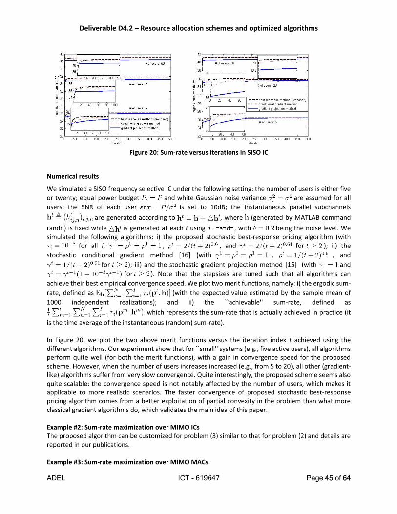
Deliverable D4.2 – Resource allocation schemes and optimized algorithms
ADEL ICT - 619647 Page 45 of 64
Figure 20: Sum-rate versus iterations in SISO IC
Numerical results
We simulated a SISO frequency selective IC under the following setting: the number of users is either five or twenty; equal power budget and white Gaussian noise variance are assumed for all
users; the SNR of each user is set to 10dB; the instantaneous parallel subchannels
are generated according to , where (generated by MATLAB command
randn) is fixed while is generated at each t using , with being the noise level. We simulated the following algorithms: i) the proposed stochastic best-response pricing algorithm (with
for all i, , , and for ); ii) the
stochastic conditional gradient method [16] (with , , and
for ); iii) and the stochastic gradient projection method [15] (with and
for ). Note that the stepsizes are tuned such that all algorithms can
achieve their best empirical convergence speed. We plot two merit functions, namely: i) the ergodic sum-
rate, defined as (with the expected value estimated by the sample mean of
1000 independent realizations); and ii) the ``achievable'' sum-rate, defined as
which represents the sum-rate that is actually achieved in practice (it
is the time average of the instantaneous (random) sum-rate). In Figure 20, we plot the two above merit functions versus the iteration index t achieved using the different algorithms. Our experiment show that for ``small'' systems (e.g., five active users), all algorithms perform quite well (for both the merit functions), with a gain in convergence speed for the proposed scheme. However, when the number of users increases increased (e.g., from 5 to 20), all other (gradient-like) algorithms suffer from very slow convergence. Quite interestingly, the proposed scheme seems also quite scalable: the convergence speed is not notably affected by the number of users, which makes it applicable to more realistic scenarios. The faster convergence of proposed stochastic best-response pricing algorithm comes from a better exploitation of partial convexity in the problem than what more classical gradient algorithms do, which validates the main idea of this paper. Example #2: Sum-rate maximization over MIMO ICs The proposed algorithm can be customized for problem (3) similar to that for problem (2) and details are reported in our publications. Example #3: Sum-rate maximization over MIMO MACs

Deliverable D4.2 – Resource allocation schemes and optimized algorithms
ADEL ICT - 619647 Page 46 of 64
We consider now the sum-rate maximization problem over MIMO MACs, as defined in (4). Define
A natural choice for the best-response of each user i is:
(13)
and is updated as while
.
Note that since the instantaneous sum-rate function is jointly concave in
for any , the ergodic sum-rate function is concave in 's, and thus the proposed algorithm will converge to the global optimal solution of (4). To the best of our knowledge, this is the first example of stochastic approximation algorithm based on best-response dynamics rather than gradient responses.
Figure 21: Sum-rate versus iterations in MIMO MAC
Numerical results. We compare the proposed best-response method (13) with the stochastic conditional gradient method [16] , and the stochastic gradient projection method [19] . In Figure 21 we plot both the ergodic sum-rate and the achievable sum-rate versus the iteration index. The figure clearly shows that the proposed algorithm outperforms the conditional gradient method and the gradient projection method in terms of convergence speed, and the performance gap is increasing as the number of users increases. This is because the proposed algorithm is a best-response type scheme, which thus explores the concavity of each users' rate function better than what gradient methods do. Note also the good scalability of the proposed best-response method.
2.2 Baseline distributed resource allocation algorithm
We compared, using the scenario defined in Table 1, the performance of the frequency agile centralized scheme with a distributed algorithm, proposed under the Task T4.2.
In the distributed algorithm, we assume the incumbents occupy channels they know are not in use by the other incumbents, while the LSA licensees are allocated the available frequencies randomly, i.e. they sense the channels randomly, and choose the first channel that they determine that is available. Under these circumstances, it may happen that a LSA licensee is using a frequency and may have to stop transmitting because the incumbent suddenly appeared on that frequency, although frequencies are still available.

Deliverable D4.2 – Resource allocation schemes and optimized algorithms
ADEL ICT - 619647 Page 47 of 64
Once again, we assume the channels as perfect, that is, each of them is occupied or idle, and this decision is 100% correct.
After translating the algorithm rules to a continuous time and homogeneous Markov chain, we were able to the get the following results in terms of blocking and dropping probabilities.
Figure 22: Random allocation (fixed and/or distributed)
From the pictures above, we extract the following conclusions: in the considered scenario, the distributed frequency allocation algorithm also exhibit some opportunities to share the band under the LSA approach that result in a probability of refusing a licensee request lower than 5% and a probability of dropping a licensee allocation lower than 0.5%.
More importantly, when comparing the distributed algorithm performance, with the performance of the centralized algorithm, we saw that in terms of dropping probabilities, as expected, the centralized algorithm is better than the distributed one. Though, one unexpected observation also arised: the blocking probability of the distributed algorithm is better than the blocking probability of the centralized algorithm. This is explained by the fact, that by having more LSA licensees that are dropped, the average occupation of the band will be lower, and by that fact, when more licensees try to get spectrum, there will be less chances of it being entirely occupied.
We stress the fact that this behavior was observed when we consider incumbent and licensees using the same channel bandwidth. In the future, we intend to compare the behavior of both algorithms for different incumbent and licensees bandwidths. In addition, we intend to extend the algorithms to include spatial dimension.
Future Work
In the future we intend to compare the behavior of the centralized and distributed algorithms for different incumbent and licensees’ bandwidth combinations. In addition, we intend to extend the algorithms to include spatial dimension.
1
2
3
4
5
10 20 30 40 50
2
PBlock
licensees
1
0
0.05
0.1
0.15
1
2
3
4
5
10 20 30 40 50
2
PDrop
licensees
1
0.01
0.02
0.03
0.04
0.05
0.06
0.07
0.2
0.4
0.6
0.8
1
1 2 3 4 5
2
PBlock
licensees
1
0.05
0.1
0.15
0.2
0.25
0.3
0.2
0.4
0.6
0.8
1
1 2 3 4 5
2
PDrop
licensees
1
0.02
0.04
0.06
0.08
Random allocation (fixed and/or distributed)N
1=6 incumbents, N
2=12 licensees, 1/
1=1.0 hours, 1/
2=0.2 hours
Random allocation (fixed and/or distributed)N
1=6 incumbents, N
2=12 licensees,
1=132.0 requests/week,
2=1608.0 requests/week

Deliverable D4.2 – Resource allocation schemes and optimized algorithms
ADEL ICT - 619647 Page 48 of 64
2.3 LSA Distributed MAC Protocol
We consider the small cells scenario where different eNBs share one or multiple LSA channels under the control of a central macro base station (BS). UEs are attached to the eNBs. The BS is responsible of only dictating to eNBs which LSA channels are available while access decisions are made in a distributed manner by eNBs.
In a classical frequency allocation scheme, multiple cells may use the same channel only if all UEs of each cell do not interfere with any UEs of the other ones, reducing hence the spatial reuse possibilities of the spectrum. Moreover, dedicating a LSA band to each small cell is less efficient than sharing all available bands among all cells as it’s more robust against changes of LSA bands availabilities. A distributed channel access scheme, on UE level, is then more preferable as per node based frequency reuse is less constrained than per cell based frequency reuse. This solution is also in line with the objective of having D2D communications capability within the coming 5G standard.
The IEEE802.11 DCF protocol is the most popular distributed access scheme but it operates only on single channel. More importantly, it suffers from severe performance degradation in multihop network topologies.
2.3.1 Inefficiency of the IEEE802.11 DCF Function in multihop networks
2.3.1.1 The Masked Node Problem
The RTS/CTS mechanism can prevent DATA packet collisions when every node in the vicinity of the sender and the receiver hears at least one control packet and defers transmission appropriately. In ad hoc networks, this assumption does not hold in general. Neighboring nodes are often unable to receive the control packets because they are masked by ongoing transmissions from other nodes near them. This means that the RTS/CTS mechanism does not generally prevent DATA packet collisions, even if the RTS/CTS handshake is performed successfully between a sender and a receiver [20] . Since DATA packet collisions reduce throughput and increase delay, masked nodes may significantly affect network performance.
Figure 23: The masked node problem of IEEE802.11 DCF protocol

Deliverable D4.2 – Resource allocation schemes and optimized algorithms
ADEL ICT - 619647 Page 49 of 64
In Figure 23, node C is masked from node B as it cannot receive its CTS message because node D is already transmitting in its range. Indeed, if some node in the neighboring of the sender does not correctly receive the RTS message due to collision, it must delay its future transmission attempt for EIFS time. The EIFS duration is larger than the time needed by the sender to, eventually, receive the CTS massage, and to start the data transmission. After EIFS, the masked node performs carrier sensing. In case of data transmission, it will delay its channel access; otherwise, it is free to initiate its handshaking.
At the receiver side, unless the use of busy tone to prevent masked node for accessing the channel, we need to improve the protocol in order to ensure reliable transmission of the CTS message.
In order to limit the impact of the masked node problem, The CSR is made in general much higher than the transmitting range. Hence, even if a CTS message is not correctly received by some masked nodes, the probability that they may sense the DATA packet transmission, and so delay their transmissions, is higher. This may reduce the impact of the masked node problem but at the expense of lower channel spatial reuse.
2.3.1.2 Impact of the masked node problem on the performances of IEEE 802.111 DCF
The inter-node visibility in multihop network impacts greatly the performance of distributed channel access schemes. We define then as input parameter the mean node visibility ratio that we define as
𝑀𝑁𝑉𝑅 =∑ |𝑁𝑖|𝑁
𝑖=1
𝑁(𝑁 − 1)
Where 𝑁𝑖 is the set of nodes in the range of node I and |𝑁𝑖| its cardinal.
We consider network size of N=50 and random topology realizations. We vary the 𝑀𝑁𝑉𝑅 between 0.2 and 1 and we consider the IEEE 802.11 DCF protocol with RTS/CTS handshaking and binary exponential backoff (BEB) scheme with different values of initial contention window W0 and maximal contention window Wmax.
Figure depicts the achieved network channel use rate Vs. MNVR. We observe that the DCF protocol performs relatively well when the networks is weakly or strongly connected but undergoes severe performance degradation in intermediate connectivity situations. Indeed, in weakly connected situations, channel reuse is still possible as nodes are widely separated in space even with the masked node problem. In strongly connected situations, the masked problem is avoided as almost all nodes can receive either RTS or CTS messages so that there is no channel reuse. The masked node problem appears clearly in intermediate connectivity situations however, as channel reuse is possible but the protocol fails to achieve it successfully.

Deliverable D4.2 – Resource allocation schemes and optimized algorithms
ADEL ICT - 619647 Page 50 of 64
Figure 24: Channel use rate vs. MNVR for IEEE802.11 DCF
Figure 24 shows the network channel use rate Vs. network size N. Many topology realizations of each network size are made with MNVR varying from 0.1 and 1. We observe then that the performance of the DCF protocol decreases with N. Indeed, with increasing network size, channel reuse possibility increases but the protocol fails dramatically to benefit from it.
Figure 25: Channel use rate vs. network size for IEEE802.11 DCF
2.3.2 Synchronized Acknowledgment Random Access MAC Protocol
We introduce a new distributed MAC protocol named Synchronized Acknowledgment Random Access MAC (SA-RA MAC) that solves, in its single channel version, efficiently the hidden node problem without introducing the masked node problem. In its multichannel version, the protocol solves also the exposed node problem and allows a complete channel reuse.
2.3.2.1 Protocol description
We consider a synchronous network with TDMA access. Each frame is composed of (L+2) slots, and each slot is composed of 2 mini-slots (Figure 26)
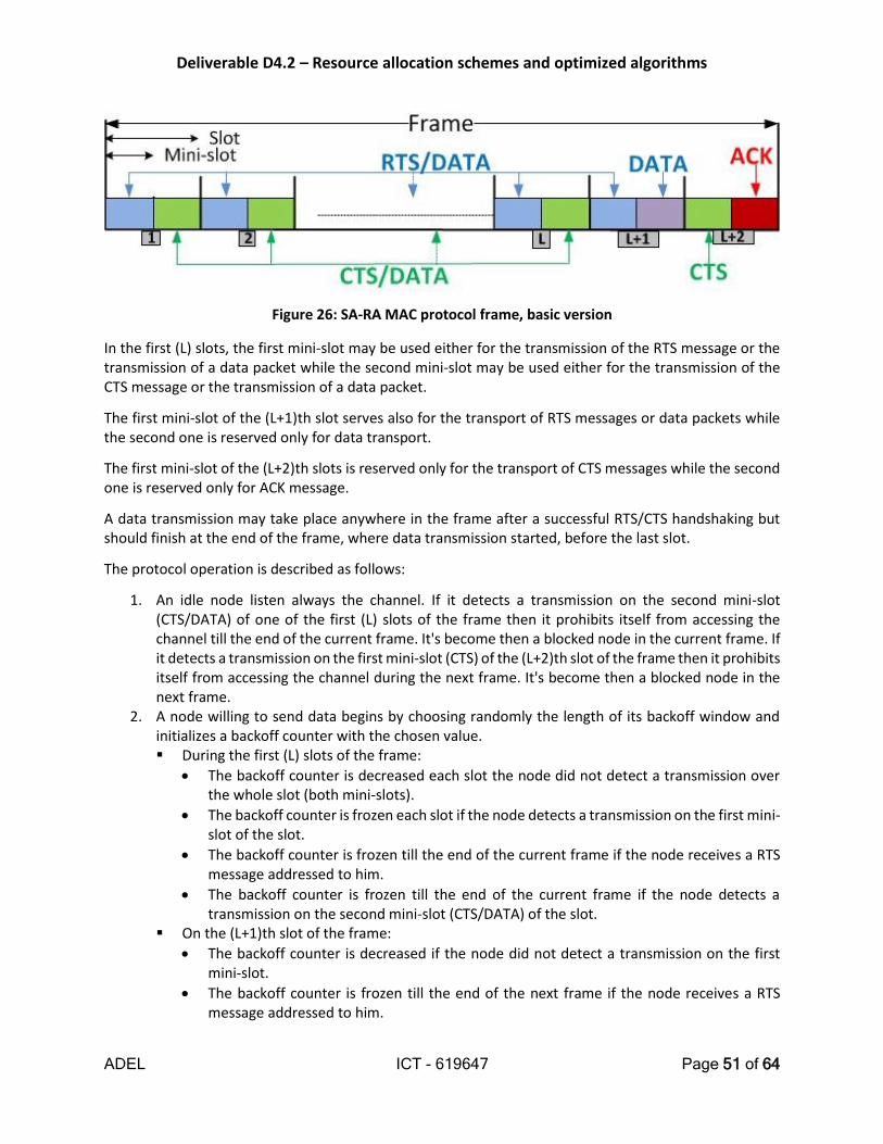
Deliverable D4.2 – Resource allocation schemes and optimized algorithms
ADEL ICT - 619647 Page 51 of 64
Figure 26: SA-RA MAC protocol frame, basic version
In the first (L) slots, the first mini-slot may be used either for the transmission of the RTS message or the transmission of a data packet while the second mini-slot may be used either for the transmission of the CTS message or the transmission of a data packet.
The first mini-slot of the (L+1)th slot serves also for the transport of RTS messages or data packets while the second one is reserved only for data transport.
The first mini-slot of the (L+2)th slots is reserved only for the transport of CTS messages while the second one is reserved only for ACK message.
A data transmission may take place anywhere in the frame after a successful RTS/CTS handshaking but should finish at the end of the frame, where data transmission started, before the last slot.
The protocol operation is described as follows:
1. An idle node listen always the channel. If it detects a transmission on the second mini-slot (CTS/DATA) of one of the first (L) slots of the frame then it prohibits itself from accessing the channel till the end of the current frame. It's become then a blocked node in the current frame. If it detects a transmission on the first mini-slot (CTS) of the (L+2)th slot of the frame then it prohibits itself from accessing the channel during the next frame. It's become then a blocked node in the next frame.
2. A node willing to send data begins by choosing randomly the length of its backoff window and initializes a backoff counter with the chosen value. During the first (L) slots of the frame:
The backoff counter is decreased each slot the node did not detect a transmission over the whole slot (both mini-slots).
The backoff counter is frozen each slot if the node detects a transmission on the first mini-slot of the slot.
The backoff counter is frozen till the end of the current frame if the node receives a RTS message addressed to him.
The backoff counter is frozen till the end of the current frame if the node detects a transmission on the second mini-slot (CTS/DATA) of the slot.
On the (L+1)th slot of the frame:
The backoff counter is decreased if the node did not detect a transmission on the first mini-slot.
The backoff counter is frozen till the end of the next frame if the node receives a RTS message addressed to him.
Deliverable D4.2 – Resource allocation schemes and optimized algorithms
ADEL ICT - 619647 Page 52 of 64
On the (L+2)th slot of the frame:
The backoff counter is decreased if the node did not detect a transmission on the first mini-slot.
The backoff counter is frozen till the end of the next frame if the node detects a transmission on the first mini-slot, otherwise it's frozen only during the slot.
3. The source node sends a RTS message to its destination when the backoff counter expires. This transmission take place on: The first mini-slot of the slot following the expiration of the backoff counter if the expiration
occurs during the first (L) slots of the frame. The first mini-slot of the next frame if the backoff counter expires in the (L+1)th slot of the
current frame. 4. If the destination node is not blocked and receives correctly the RTS message then it sends back
a CTS message to the source node to indicate its availability for data reception. This transmission take place on: The second mini-slot of the slot where the RTS was sent if the slot is among the first $L$ slots
of the frame. The first mini-slot of the slot (L+2) if the RTS was sent in the (L+1)th slot.
5. If the source node receive correctly the CTS message then the data transmission starts in: The slot following the RTS/CTS handshaking in case the handshaking took place in one of the
first (L) slots of the frame. The first slot of the next frame if the handshaking took place in the (L+1)th and the (L+2)th
slots of the current frame.
Thus, the data transmissions may start in any of the first (L+1) slots of the frame after a successful RTS/CTS handshaking but should terminate all at the end of frame before the last slot.
If the source node did not receive the CTS message then it may either abort or retry again the channel acquisition by repeating steps 2 to 5 for some predefined number of attempts.
6. The destination node sends an ACK message at the end of data transmission in the last mini-slot of the frame where data transmission (not necessarily the same frame as for the RTS/CTS handshaking) starts.
Figure 27 illustrates the operation of the SA-RA MAC protocol in the masked node scenario depicted in Figure. We can see that synchronizing the end of data transmissions from nodes A and D avoids collision of node C's RTS with node A data transmission. The SA-RA MAC protocol succeeds then to resolve efficiently the hidden terminal problem without the side effect of masked node problem, it allows then safe channel reuse.
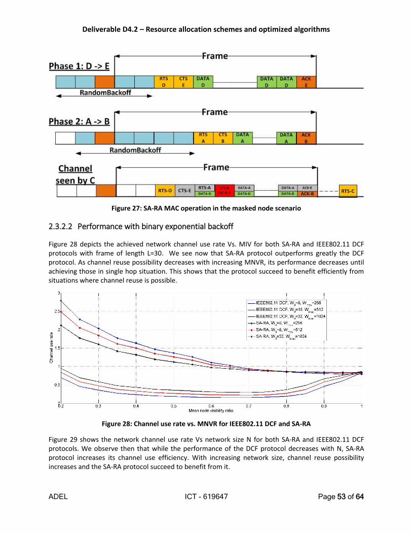
Deliverable D4.2 – Resource allocation schemes and optimized algorithms
ADEL ICT - 619647 Page 53 of 64
Figure 27: SA-RA MAC operation in the masked node scenario
2.3.2.2 Performance with binary exponential backoff
Figure 28 depicts the achieved network channel use rate Vs. MIV for both SA-RA and IEEE802.11 DCF protocols with frame of length L=30. We see now that SA-RA protocol outperforms greatly the DCF protocol. As channel reuse possibility decreases with increasing MNVR, its performance decreases until achieving those in single hop situation. This shows that the protocol succeed to benefit efficiently from situations where channel reuse is possible.
Figure 28: Channel use rate vs. MNVR for IEEE802.11 DCF and SA-RA
Figure 29 shows the network channel use rate Vs network size N for both SA-RA and IEEE802.11 DCF protocols. We observe then that while the performance of the DCF protocol decreases with N, SA-RA protocol increases its channel use efficiency. With increasing network size, channel reuse possibility increases and the SA-RA protocol succeed to benefit from it.
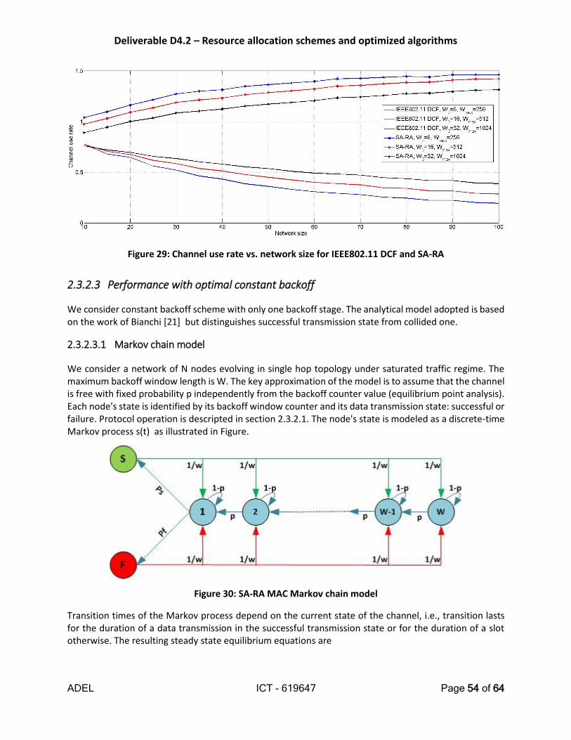
Deliverable D4.2 – Resource allocation schemes and optimized algorithms
ADEL ICT - 619647 Page 54 of 64
Figure 29: Channel use rate vs. network size for IEEE802.11 DCF and SA-RA
2.3.2.3 Performance with optimal constant backoff
We consider constant backoff scheme with only one backoff stage. The analytical model adopted is based on the work of Bianchi [21] but distinguishes successful transmission state from collided one.
2.3.2.3.1 Markov chain model
We consider a network of N nodes evolving in single hop topology under saturated traffic regime. The maximum backoff window length is W. The key approximation of the model is to assume that the channel is free with fixed probability p independently from the backoff counter value (equilibrium point analysis). Each node's state is identified by its backoff window counter and its data transmission state: successful or failure. Protocol operation is descripted in section 2.3.2.1. The node's state is modeled as a discrete-time Markov process s(t) as illustrated in Figure.
Figure 30: SA-RA MAC Markov chain model
Transition times of the Markov process depend on the current state of the channel, i.e., transition lasts for the duration of a data transmission in the successful transmission state or for the duration of a slot otherwise. The resulting steady state equilibrium equations are

Deliverable D4.2 – Resource allocation schemes and optimized algorithms
ADEL ICT - 619647 Page 55 of 64
1. 𝜋𝑊 =𝜋𝑠+𝜋𝑓
𝑊
2. 𝜋𝑖 = 𝜋𝑠+𝜋𝑓
𝑊+ 𝜋𝑖+1𝑃 ; 𝑖 = 1, … , 𝑊 − 1
3. 𝜋𝑠 = 𝜋1𝑃[1 − 𝜋1]𝑁−1
4. 𝜋𝑓 = 𝜋1𝑃(1 − [1 − 𝜋1]𝑁−1)
Where
𝑃 = [1 − 𝜋𝑠 − 𝜋𝑓]𝑁−1
From Equations 1 and 2 and the normalizing equation 𝜋𝑠 + 𝜋𝑓 + ∑ 𝜋𝑖𝑊𝑖=1 = 1 we get
[1 − 𝜋𝑠 − 𝜋𝑓]𝑁
=𝑊 + 1
2(𝜋𝑠 + 𝜋𝑓)
From Equations 3 and 4 we get
𝜋𝑠 + 𝜋𝑓 = 𝜋1[1 − 𝜋𝑠 − 𝜋𝑓]𝑁−1
≈ 𝜋1𝑒−(𝑁−1)(𝜋𝑠+𝜋𝑓)
≈𝐿𝑤0((𝑁 − 1)𝜋1)
𝑁 − 1
Where 𝐿𝑤0 is the principal branch of the Lambert W function.
We get then
𝜋𝑠 ≈ 𝐿𝑤0((𝑁−1)𝜋1)
𝑁−1𝑒−(𝑁−1)𝜋1
The network channel use is given as
𝐶𝑢 =𝑁𝜋𝑠𝑇𝑠
𝑁𝜋𝑠(𝑇𝑠 + 1) + 1
𝑇𝑠 is the average duration of successful data transmission without taking into account the 2 slots used for the RTS/CTS/ACK handshaking.
Taking into account that a successful data transmission may take place anywhere in a frame, 𝑇𝑠 is given as
𝑇𝑠 =(𝐿 + 1)𝑃𝑠𝑠(𝐿 + 1) + ∑ 𝑃𝑠𝑠(𝑘)(𝐿 + 1 − 𝑘)𝐿
𝑘=1
𝑃𝑓𝑠
Where 𝑃𝑠𝑠(𝑘) is the probability that data transmission starts at the (k+1)th slot(k=1,…,L), or at the 1st slot( k=L+1).
𝑃𝑠𝑠(𝐿 + 1) =𝑁𝜋𝑠(1−𝑁𝜋𝑠)𝐿
1+𝑁𝜋𝑠(1−𝑁𝜋𝑠)𝐿

Deliverable D4.2 – Resource allocation schemes and optimized algorithms
ADEL ICT - 619647 Page 56 of 64
𝑃𝑠𝑠(𝑘) = [1 − 𝑃𝑠𝑠(𝐿 + 1)]𝑁𝜋𝑠(1 − 𝑁𝜋𝑠)𝑘−1 ; 𝑘 = 1, … , 𝐿 𝑃𝑓𝑠 = ∑ 𝑃𝑠𝑠(𝑘)𝐿+1
𝑘=1
The protocol efficiency is monotonically increasing with the increase in data transmission duration. We define the frame acquisition efficiency (FAE) as the ratio of the average data transmission duration 𝑇𝑠 over the frame length (L+2). Figure depicts the FAE vs. the network probability of data transmission N𝜋𝑠 for L=30. We observe then that for low data transmission probability, the average 𝑇𝑠 is half the frame length meaning that only half of the frame is used. This occurs in situations when the access collision probability is very high or when the traffic load is very low.
Figure 31: Frame acquisition efficiency Vs. Probability of success
Indeed, the optimization of the backoff window aims to avoid the first situations by reducing the channel access collision probability.
It has been shown in [22] that BEB window schemes suffers from unfairness and that optimal constant window backoff scheme outperforms BEB ones in terms of both efficiency and fairness.
The channel use Cu is maximal when 𝜋𝑠 is maximal. Making the change of variable 𝑧 = (𝑁 − 1)𝜋𝑠 we get
𝜑𝜋𝑠
𝜑𝑧= 0 → 𝑧𝐿𝑤0(𝑧) + 𝑧 = 1
By definition of the Lambert W function we have that 𝐿𝑤0(𝑧) = 𝑡 ↔ 𝑡𝑒𝑡 = 𝑧, which implies
𝜑𝜋𝑠
𝜑𝑧= 0 → 𝑡2𝑒𝑡 + 𝑡𝑒𝑡 = 1 → 𝑡𝑜𝑝 ≈ 0.44413
The optimal values of 𝜋1 and W are then
𝜋1𝑜𝑝 =𝑡𝑜𝑝𝑒𝑡𝑜𝑝
𝑁−1

Deliverable D4.2 – Resource allocation schemes and optimized algorithms
ADEL ICT - 619647 Page 57 of 64
𝑊𝑜𝑝 =2(𝑁−1)(1−
𝑡𝑜𝑝
𝑁−1)
𝑁
𝑡𝑜𝑝− 1
We plot in Figure 32 the FAE vs. the frame length in saturated traffic regime with the employment of the optimal backoff window. We observe then that the achieved frame acquisition efficiency is high and increases naturally with the increase of the frame length.
Figure 32: Frame acquisition efficiency Vs. frame length
In Figure 33 we compare the performance of the optimal backoff scheme to the BEB one in term of efficiency and we observe that the optimal backoff scheme shows better results as it adapts to the network size.
Figure 33: Optimal constant backoff scheme VS. BEB scheme

Deliverable D4.2 – Resource allocation schemes and optimized algorithms
ADEL ICT - 619647 Page 58 of 64
2.3.2.4 Performance in non-saturated regimes
The SA-RA protocol, as defined earlier, offers to each node that succeeded the RTS/CTS handshaking to access the channel till the end of the frame. In saturated regime this is not problematic as nodes always have enough data to fill the frame. In real scenarios however, saturated regimes appear only in extreme and temporary situations regarding the quasi systematic presence of admission control mechanisms that prevent and resolve them.
We consider the performance of SA-RA MAC protocol for finite load homogeneous traffics. Packet arrival for node k follows a Poisson distribution of mean intensity 𝜇𝑘 of length geometrically distributed with mean 𝜎𝑘 slots. We simulate multiple runs of the protocle with parameters 𝜎𝑘 =L/2 Slots and 𝜇𝑘 varying between {0.1, … ,1}2/(𝐿𝑁) making the overall network arrival rate varying between 0.1 and 1.
We plot in Figure 34 the loss rate in term of unused data slot per when varying the traffic arrival rate for frame of length L=30 and network of size N=30. We observe that the protocol exhibits high wasting of granted data slot for weak to moderate traffic intensity.
Figure 34: Unused slot rate in SA-RA MAC Vs. packet arrival rate
To overcome this problem, we introduce in the next section a mini-frame version of the protocol that allows it to adapt better to traffic load intensity.
2.3.2.4.1 Mini-frame version In this version, the frame of the SA-RA MAC protocol is divided into (M+1) mini frames. The first M mini frames are optional while the last one is mandatory and has the same structure as the frame of basic version of the protocol. Each mini frame is composed of (L+2) slots, and each slot is composed of 2 mini slots. As in the basic version, in the first L slots, the first mini slot may be used either for the transmission of the RTS message or the transmission of a data packet while the second mini-slot may be used either for the transmission of the CTS message or the transmission of a data packet.
The first mini-slot of the (L+1)th slot serves for the transport of RTS messages or data packets while the second one is reserved only for data packets transport.
The use of the last slot is as follows:
In the first M mini frames, the first mini slot may transport either CTS message or P-ACK (Partial ACK) messages. The second one is reserved only for ACK messages.

Deliverable D4.2 – Resource allocation schemes and optimized algorithms
ADEL ICT - 619647 Page 59 of 64
In the last mini frame, the first mini-slot is reserved only for the transport of CTS messages while the second one is reserved only for ACK messages.
Hence, a data transmission may take place over one or multiple mini frames but should mandatory stop at the end of one of the mini frames belonging to the frame where data transmission started.
Figure 35 shows the frame structure of the mini-frames version of the protocol.
Figure 35: SA-RA MAC protocol, mini-frames version
The protocol operation is described as follows:
1. An idle node listen always the channel. If it detects a transmission on the second mini-slot (CTS/DATA) of one of the first L slots of a mini frame then it prohibits itself from accessing the channel till the end of the mini frame. It's become then a blocked node in the current mini frame. If it detects a transmission on the first mini-slot (CTS) of the (L+2)th slot of the mini frame then it prohibits itself from accessing the channel during the next mini frame. It's become then a blocked node in the next mini frame.
2. A node willing to send data begins by choosing randomly the length of its backoff window and initializes a backoff counter with the chosen backoff window value.
During the first L slots of the mini frame:
The backoff counter is decreased each slot the node did not detect a transmission over the whole slot (both mini-slots).
The backoff counter is frozen each slot if the node detects a transmission on the first mini-slot of the slot.
The backoff counter is frozen till the end of the data transmission if the node receives a RTS message destinated to him. The end of the data transmission is indicated in the RTS message.
The backoff counter is frozen till the end of the mini frame if the node detects a transmission on the second mini-slot (CTS/DATA) of the slot.
On the (L+1)th slot of the mini frame:
The backoff counter is decreased if the node did not detect a transmission on the first mini-slot.
The backoff counter is frozen each slot if the node detects a transmission on the first mini-slot of the slot.
The backoff counter is frozen till the end of the data transmission if the node receives a RTS message destinated to him.
On the (L+2)th slot of the mini frame:

Deliverable D4.2 – Resource allocation schemes and optimized algorithms
ADEL ICT - 619647 Page 60 of 64
The backoff counter is frozen till the end of the next mini frame if the node detects a transmission on the first mini-slot, otherwise it's frozen only during the slot.
3. The source node sends a RTS message to its destination when the backoff counter expires. This transmission take place on:
The first mini slot of the slot following the expiration of the backoff counter if the expiration occurs during the first $L$ slots of the mini frame.
The first mini slot of the next mini frame if the backoff counter expires in the (L+1)th slot of the mini frame.
4. If the destination node is not blocked and receives correctly the RTS message then it sends back a CTS message to the source node to indicate its availability for data reception. This transmission takes place on:
The second mini slot of the slot where the RTS was sent if the slot is among the first L slots of the mini frame.
The first mini slot of the slot (L+2) if the RTS was sent in the (L+1)th slot of the mini frame 5. If the source node receive correctly the CTS message then the data transmission starts in:
The slot following the RTS/CTS handshaking if the handshaking has took place in one of the first L slots of the mini frame.
The first slot of the next mini frame if the handshaking took place in the (L+1)th and the (L+2)th slots of the mini frame.
Thus, the data transmissions may start in any of the first (L+1) slots of the mini frames after a successful RTS/CTS handshaking but should mandatory terminate all at the end of one of the mini frames belonging to the frame where the data transmission started.
If the source node did not receive the CTS message then it may either abort or retry again the channel acquisition by repeating steps 2 to 5 for some predefined number of attempts.
6. The destination node sends an ACK message at the end of data transmission in the last mini-slot of the last mini frame and P-ACK messages on all other intermediate mini frames.
We plot in Figure 36 the loss rate in term of unused data slot for both version of SA-RA MAC protocol with the same parameters as in the previous section. We observe now that the mini-frame version exhibit far less waste the use of the channel even for low traffic load.
Figure 36: Unused slot rate of SA-RA MAC mono-frame and multi-frame Vs. packet arrival rate

Deliverable D4.2 – Resource allocation schemes and optimized algorithms
ADEL ICT - 619647 Page 61 of 64
2.4 Frequency ALOHA for Small Cells: Throughput vs. Coverage Trade-Off
We assume that 𝑀 Small-Cell Base Station (SCBS) can access a given spectrum BW, which is divided in 𝑁 sub-bands. Each SCBS can assess only one of the 𝑁 sub-bands, chosen independently of the other SCBSs. This has a two-fold effect. On the one hand, it reduces the interference from the neighbouring cells, on the other hand it reduces the reuse of spectrum. This frequency allocation scheme is also known as Frequency ALOHA [30].
In this context, our contribution consists in evaluating the area spectral efficiency vs coverage trade-off as a function of the cell-density and of the number of bands 𝑁 that can be obtained in a small-cell network by means of frequency ALOHA. Moreover, we investigate the effect of the path-loss model on the performance of the dense small-cell network.
We assume the SCBSs are distributed according to a Spatial Poisson Point Process and each cell has at least one users to serve. The users are uniformly distributed and are served with full-buffer traffic.
In the problem formulation, we assume the path-loss can be either single-slope (i.e., it is in the form 𝑃𝐿(𝑑) = 𝐴𝑆𝐿 + 𝐵𝑆𝐿 log10 𝑑 in the logarithm domain) or dual-slope with probability of Line-of-Sight (LOS) or Non-Line-of-Sight (NLOS). The dual-slope path-loss model is given below:
𝑃𝐿(𝑑)(𝑑) = {𝑃𝐿(𝑑) = 𝐴𝐿𝑂𝑆 + 𝐵𝐿𝑂𝑆 log10 𝑑 with probability pLOS(d)
𝑃𝐿(𝑑) = 𝐴𝑁𝐿𝑂𝑆 + 𝐵𝑁𝐿𝑂𝑆 log10 𝑑 with probability 1 − pLOS(d)
Where
pLOS(d) = 0.5 − min (0.5, 5exp [−−𝑑0
𝑑]) + min (0.5, 5exp [−
−𝑑
𝑑1]).
The values of 𝐴𝐿𝑂𝑆, 𝐴𝑁𝐿𝑂𝑆, 𝐵𝐿𝑂𝑆, 𝐵𝑁𝐿𝑂𝑆, 𝑑0 and 𝑑1 for this model are given in the standard 3GPP [28]. The small-scale fading has Rayleigh distribution.
The frequency allocation scheme given above is apt to be used in small-cell networks, as it does not required any coordination among base stations. Frequency ALOHA is a frequency allocation scheme that runs in a distributed manner. It achieves interference mitigation on a probabilistic manner and, therefore, has little implementation complexity involved. In case a network operator had the need to change the frequency reuse factor of its network, this could be achieved by broadcasting the information regarding the number of bands each cell is allowed to use. The area spectral efficiency and the coverage of the network can be computed using a mathematical tool based on stochastic geometry. The detail of this formulation can be found in [29]. The parameters values for the channel model are reported in
Table 2. We assume the network to be in the interference limited regime, i.e., the transmit power is high enough so that the thermal noise power can be discarded.

Deliverable D4.2 – Resource allocation schemes and optimized algorithms
ADEL ICT - 619647 Page 62 of 64
Table 2: Channel model parameters.
Parameter Value
𝐴𝐿𝑂𝑆 103.8
𝐴𝑁𝐿𝑂𝑆 145.4
𝐵𝐿𝑂𝑆 2.09
𝐵𝑁𝐿𝑂𝑆 3.75
𝑑0 0.156 km
𝑑1 0.3 km
𝐴𝑆𝐿 140.7
𝐵𝑆𝐿 36.7
The results of this trade-off are shown in Figure 37, where we plotted the network coverage against the ASE for different frequency reuse factors and base station densities.
Figure 37: ASE vs coverage trade-off for frequency reuse. The trade-off curves have been plotted for BS density equal to 10, 20, 50, 100, 200, 500, 1000, 2000, 5000, 10000 BSs/km2, and compare the combined LOS/NLOS model with the single-slope (SL) one.
Firstly, we focus on the LOS/NLOS propagation; we can notice from this plot that, if we fix the SCBS density, higher frequency reuse factors enhance the network coverage but, on the other hand, determine a drop of the ASE. This is in line with what one would expect from frequency reuse. Nonetheless, if we have no constraint in the choice of the BS density, the ASE vs coverage trade-off improves as the frequency reuse

Deliverable D4.2 – Resource allocation schemes and optimized algorithms
ADEL ICT - 619647 Page 63 of 64
factor 𝑁 increases. In fact, the trade-off curve we obtain for a given reuse factor 𝑁 lies on the top-right hand side with respect to the curve for reuse factor 𝑁 − 1. This means that, by increasing the reuse factor and the base station density at the same time, it is possible to achieve better performance than with a lower frequency reuse factors; note, though, that this is true when there is no constraint in terms of BS density. This is actually a surprising results, as one might think that increasing the frequency reuse factor leads to a drastic drop of the area spectral efficiency, due to the usage of only one 𝑁-th of the available bandwidth. However, it turns out that the interference reduction obtained by limiting each cell spectrum usage counterbalances the spectral efficiency decrease due to this spectrum limitation and, thus, provides an overall gain in the ASE vs. coverage trade-off, as the density increases. From the plot in Fig. 1 we can conclude that frequency ALOHA turns to be a simple but effective resource management technique for dense networks, which would otherwise face serious coverage issues due to the effect of LOS/NLOS propagation.
By looking at the single slope path-loss curve in Figure, it appears that higher frequency reuse factors should still be preferred in order to improve the ASE vs coverage trade-off. However, unlike with the LOS/NLOS path loss, increasing the SCBS density enhances the ASE with no loss in terms of network coverage. Yet, modelling the signal propagation with the combined LOS/NLOS path loss yields different results than with the single-slope path-loss.
Conclusions
In this deliverable, we have developed various centralised and distributed resorce allocation schemes and optimized algorithms in ADEL scenarios with performance comparison, both analytically and numerically. The proposed resource allocation schemes have one or several of the notable advantages in terms of efficiency, delay, overhead and QoS guarantees. The proposed techniques can successfully carry out the dynamic and optimal resource allocation, which aligns with ADEL’s vision.
References
[1] H. Ahmadi et. al., “Substitutability of spectrum and cloud-based antennas in virtualised wireless networks,”IEEE Wireless Communications Magazine,2016 (to appear)
[2] D. P. Bertsekas, Nonlinear programming, Athena Scientific, 1999. [3] S. Boyd and L. Vandenberghe, Convex optimization, Cambridge Univ Pr, 2004. [4] N. Jindal, W. Rhee, S. Vishwanath, S. Jafar, and A. Goldsmith, “Sum Power Iterative Water-Filling for
Multi-Antenna Gaussian Broadcast Channels},'' IEEE Transactions on Information Theory, vol. 51, no. 4, pp. 1570--1580, Apr. 2005.
[5] D. P. Palomar and M. Chiang, “A tutorial on decomposition methods for network utility maximization,” IEEE Journal on Selected Areas in Communications, vol. 24, no. 8, pp. 1439--1451, Aug. 2006.
[6] G. Scutari, F. Facchinei, P. Song, D. P. Palomar, and J.-S. Pang, “Decomposition by Partial Linearization: Parallel Optimization of Multi-Agent Systems,” IEEE Transactions on Signal Processing, vol. 62, no. 3, pp. 641--656, Feb. 2014.
[7] G. Scutari, F. Facchinei, L. Lampariello, , and P. Song, “Distributed Methods for Constrained Nonconvex Multi-Agent Optimization-Part I: Theory,” Oct. 2014, submitted to IEEE Transactions on Signal Processing. [Online]. Available: http://arxiv.org/abs/1410.4754
[8] Y. Yang, G. Scutari, P. Song, and D. P. Palomar, “Robust MIMO Cognitive Radio Systems Under Interference Temperature Constraints”, IEEE Journal on Selected Areas in Communications, vol. 31, no. 11, pp. 2465--2482, Nov. 2013.
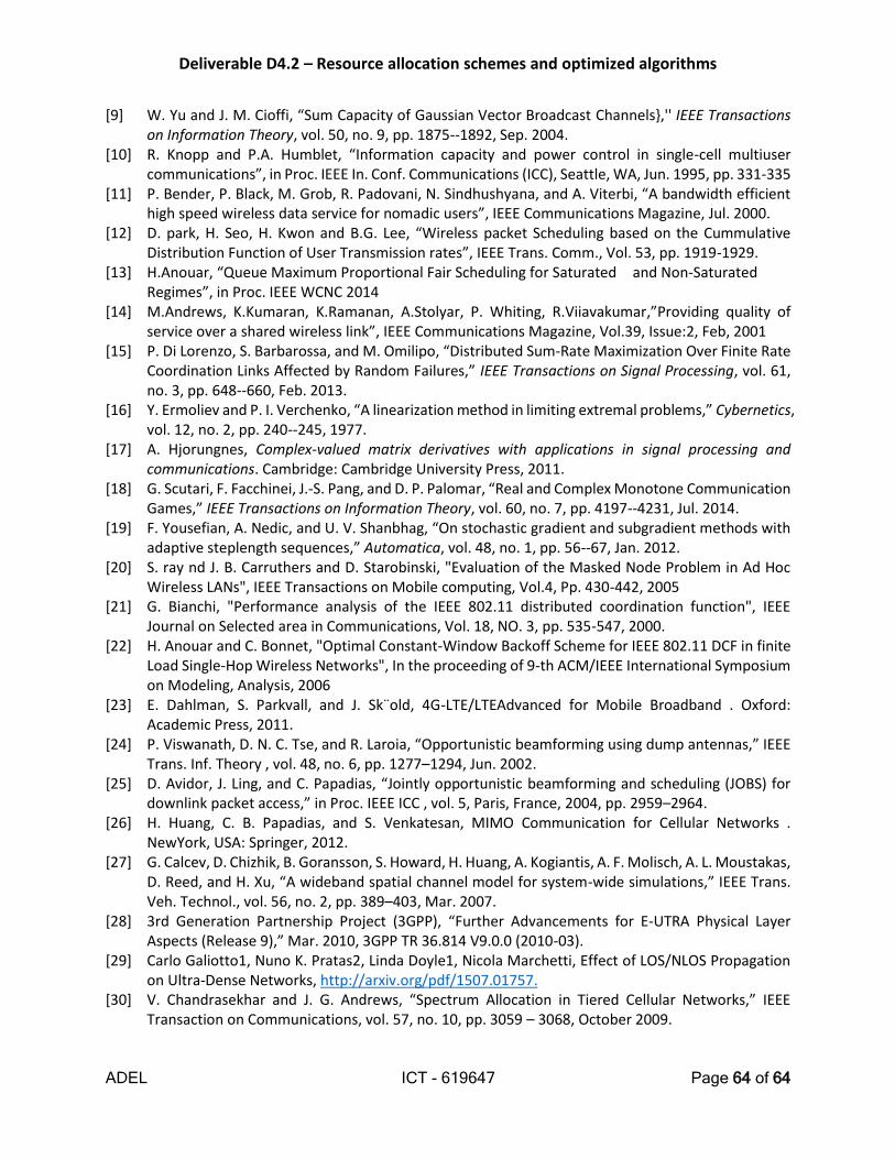
Deliverable D4.2 – Resource allocation schemes and optimized algorithms
ADEL ICT - 619647 Page 64 of 64
[9] W. Yu and J. M. Cioffi, “Sum Capacity of Gaussian Vector Broadcast Channels},'' IEEE Transactions on Information Theory, vol. 50, no. 9, pp. 1875--1892, Sep. 2004.
[10] R. Knopp and P.A. Humblet, “Information capacity and power control in single-cell multiuser communications”, in Proc. IEEE In. Conf. Communications (ICC), Seattle, WA, Jun. 1995, pp. 331-335
[11] P. Bender, P. Black, M. Grob, R. Padovani, N. Sindhushyana, and A. Viterbi, “A bandwidth efficient high speed wireless data service for nomadic users”, IEEE Communications Magazine, Jul. 2000.
[12] D. park, H. Seo, H. Kwon and B.G. Lee, “Wireless packet Scheduling based on the Cummulative Distribution Function of User Transmission rates”, IEEE Trans. Comm., Vol. 53, pp. 1919-1929.
[13] H.Anouar, “Queue Maximum Proportional Fair Scheduling for Saturated and Non-Saturated Regimes”, in Proc. IEEE WCNC 2014
[14] M.Andrews, K.Kumaran, K.Ramanan, A.Stolyar, P. Whiting, R.Viiavakumar,”Providing quality of service over a shared wireless link”, IEEE Communications Magazine, Vol.39, Issue:2, Feb, 2001
[15] P. Di Lorenzo, S. Barbarossa, and M. Omilipo, “Distributed Sum-Rate Maximization Over Finite Rate Coordination Links Affected by Random Failures,” IEEE Transactions on Signal Processing, vol. 61, no. 3, pp. 648--660, Feb. 2013.
[16] Y. Ermoliev and P. I. Verchenko, “A linearization method in limiting extremal problems,” Cybernetics, vol. 12, no. 2, pp. 240--245, 1977.
[17] A. Hjorungnes, Complex-valued matrix derivatives with applications in signal processing and communications. Cambridge: Cambridge University Press, 2011.
[18] G. Scutari, F. Facchinei, J.-S. Pang, and D. P. Palomar, “Real and Complex Monotone Communication Games,” IEEE Transactions on Information Theory, vol. 60, no. 7, pp. 4197--4231, Jul. 2014.
[19] F. Yousefian, A. Nedic, and U. V. Shanbhag, “On stochastic gradient and subgradient methods with adaptive steplength sequences,” Automatica, vol. 48, no. 1, pp. 56--67, Jan. 2012.
[20] S. ray nd J. B. Carruthers and D. Starobinski, "Evaluation of the Masked Node Problem in Ad Hoc Wireless LANs", IEEE Transactions on Mobile computing, Vol.4, Pp. 430-442, 2005
[21] G. Bianchi, "Performance analysis of the IEEE 802.11 distributed coordination function", IEEE Journal on Selected area in Communications, Vol. 18, NO. 3, pp. 535-547, 2000.
[22] H. Anouar and C. Bonnet, "Optimal Constant-Window Backoff Scheme for IEEE 802.11 DCF in finite Load Single-Hop Wireless Networks", In the proceeding of 9-th ACM/IEEE International Symposium on Modeling, Analysis, 2006
[23] E. Dahlman, S. Parkvall, and J. Sk¨old, 4G-LTE/LTEAdvanced for Mobile Broadband . Oxford: Academic Press, 2011.
[24] P. Viswanath, D. N. C. Tse, and R. Laroia, “Opportunistic beamforming using dump antennas,” IEEE Trans. Inf. Theory , vol. 48, no. 6, pp. 1277–1294, Jun. 2002.
[25] D. Avidor, J. Ling, and C. Papadias, “Jointly opportunistic beamforming and scheduling (JOBS) for downlink packet access,” in Proc. IEEE ICC , vol. 5, Paris, France, 2004, pp. 2959–2964.
[26] H. Huang, C. B. Papadias, and S. Venkatesan, MIMO Communication for Cellular Networks . NewYork, USA: Springer, 2012.
[27] G. Calcev, D. Chizhik, B. Goransson, S. Howard, H. Huang, A. Kogiantis, A. F. Molisch, A. L. Moustakas, D. Reed, and H. Xu, “A wideband spatial channel model for system-wide simulations,” IEEE Trans. Veh. Technol., vol. 56, no. 2, pp. 389–403, Mar. 2007.
[28] 3rd Generation Partnership Project (3GPP), “Further Advancements for E-UTRA Physical Layer Aspects (Release 9),” Mar. 2010, 3GPP TR 36.814 V9.0.0 (2010-03).
[29] Carlo Galiotto1, Nuno K. Pratas2, Linda Doyle1, Nicola Marchetti, Effect of LOS/NLOS Propagation on Ultra-Dense Networks, http://arxiv.org/pdf/1507.01757.
[30] V. Chandrasekhar and J. G. Andrews, “Spectrum Allocation in Tiered Cellular Networks,” IEEE Transaction on Communications, vol. 57, no. 10, pp. 3059 – 3068, October 2009.