advanced engineering computations

155

6

AdvancedEngineeringComputations

E

lectrical engineers

use filters extensively in radios, telephones, televisions, computers,

power supplies, and many other practical devices. A specific example is

the low-pass filter used in the design of a direct current (DC) power supply.

An

ideal low-pass filter

is a device that completely transmits a signal

unattenuated at all frequencies below a certain cutoff frequency and

completely blocks those frequency components of the input signal above

this cutoff frequency. The application in this chapter uses

complex phasors

(a common method used to describe a time-periodic quantity in terms of

a single complex number) and

nodal analysis

(a circuit analysis technique

described later in this chapter) to analyze an approximation to an ideal

low-pass filter. This technique is very general, and is a powerful tool for

circuit analysis. Maple’s ability to find complex-valued solutions to alge-

braic equations forms the foundation upon which the remainder of the

analysis can be completed. You will also learn Maple commands and

techniques for use with more sophisticated mathematics concepts,

including calculus and differential equations.

Low-Pass Electrical Filter

156

MAPLE V FOR ENGINEERS

aple can be used in many different branches of mathematicsincluding algebra, calculus, combinatorics, financial mathematics,graph theory, linear algebra, logic, number theory, and optimiza-

tion. The first five chapters of this module showed you how to use Mapleto solve problems requiring mainly algebra and trigonometry. In thischapter, you will see some of the ways Maple can be used to solve prob-lems that involve complex analysis, calculus, and (briefly) differentialequations. The application in this chapter shows how an electrical engi-neer uses nodal analysis to investigate some of the characteristics of alow-pass electrical filter. Recall that the bandwidth application in Chapter 3also involved the analysis of a filter. Even though there are similarities inhow engineers discuss both types of filters, the discussion in this chapteris quite different from the one presented in Chapter 3.

Although you will learn many useful techniques for solving mathemati-cal problems in this chapter, it is not comprehensive in its presentation ofMaple’s mathematical capabilities. Some of the examples and Try It! exer-cises refer to problems encountered earlier in the module. For example,the solution to the Streeter–Phelps equation that was provided in Chapter 5will now be found and verified using Maple. References to the earlier dis-cussions are provided; if you do not recall the details of a problem, pleasetake a few minutes to refresh your memory.

Several dozen packages contain collections of additional Maple com-mands. The

plots

and

student

packages have been introduced previ-ously. The

student

package will be used in the discussion of calculus(Section 6-2) and the

DEtools

package will be used to produce plots relat-ing to differential equations (Section 6-3). Other packages likely to be ofinterest to many engineers include the

linalg

package for linear algebra,the

numtheory

package for number theory, and the

inttrans

package forintegral transformation such as the Laplace and Fourier transform. Thefull list of Maple packages can be found on the online help worksheet withkeyword

index,package

.

6-1 COMPLEX NUMBERS

Maple functions and variables are, by default, assumed to be complex valued.This may seem to be an unnecessary feature for most standard computa-tions, but it is actually one of the underlying characteristics that gives Mapleits power and broad applicability. There are times, however, when thisincreased functionality interferes with some seemingly simple operations.

Basic arithmetic operations (addition, subtraction, multiplication, anddivision) are performed exactly as they would be for real-valued quanti-ties. The only difference is the use of

I

to represent the square root of

−

1,that is, . For example, the sum and product of

z

=

2

+

3

i

and

w

=

6

−

4

i

can be computed using

>

z

:=

2+3*I;

z

:= 2

+

3

I

MINTRODUCTION

I= −1

CHAPTER 6 ADVANCED ENGINEERING COMPUTATIONS

157

>

w

:=

6-4*I;

w

:= 6

−

4

I

>

SUMzw

:=

z+w;

SUMzw

:= 8

−

I

>

QUOTzw

:=

z/w;

Common commands specifically designed for use with complex-valuedobjects include

abs

,

conjugate

,

Re

, and

Im

. For expressions involvingsymbolic names, the

evalc

command is used to force the evaluation ofcomplex-valued expressions in the standard form:

x

+

I y

.

Arithmetic of Complex Numbers

Let

z

denote a complex number with real part

Rez

and imaginary part

Imz

.Similarly, let

w

=

Rew

+

i

Imw

. Find, in standard form, the

conjugate

of

z

,

z

, and the real and imaginary parts of the product

zw

.

SOLUTION

The two complex numbers are

>

z

:=

Rez

+

I*Imz;

z

:=

Rez

+

I Imz

>

w := Rew + I*Imw;

w := Rew + I Imw

The complex conjugate of z, z, simply changes the sign of the imaginarypart:

> zC := conjugate(z);

zC := Rez + I Imz

> zC := evalc( zC );

zC := Rez – I Imz

Note how evalc is used to reduce the expression into standard form.The product of z and w is

> PRODzw := z * w;

PRODzw := (Rez + I Imz) (Rew + I Imw)

QUOTzw I : = 12

EXAMPLE 6-1

158 MAPLE V FOR ENGINEERS

The real and imaginary parts of the product are

> REzw := Re( PRODzw );

REzw := ℜ ((Rez + I Imz) (Rew + I Imw))

> IMzw := Im( PRODzw );

IMzw := ℑ ((Rez + I Imz) (Rew + I Imw))

Or, in standard form,

> REzw = evalc( REzw );

ℜ ((Rez + I Imz) (Rew + I Imw)) = Rez Rew − Imz Imw

> IMzw = evalc( IMzw );

ℑ ((Rez + I Imz) (Rew + I Imw)) = Rez Imw + Imz Rew

Of course, the same information can be obtained by directly convertingthe product into standard form:

> PRODzw = evalc( PRODzw );

(Rez + I Imz) (Rew + I Imw) = Rez Rew − Imz Imw + I (Rez Imw + Imz Rew)

Other operations work in a similar manner. One point that should beemphasized is that it is important to use built-in Maple commands forstandard operations whenever possible. This is the point of the next Try It!exercise.

The modulus, or magnitude, of a complex number is the square root of the product of the number and its conjugate. Compute the modulus of the complex numbers z and z w both from the definition and using Maple’s abs command. Explain and resolve any differences in the appearance of the results.

You may have noticed that expressions returned by evalc (in standardform) are valid only when the real and imaginary parts of z and w (that is,Rez, Imz, Rew, Imw) are real–valued. In fact, the fundamental assumptionmade by evalc is that unassigned variables represent real-valued quantities.For example, when neither a nor b is assigned a value, evalc( Re( a+I*b ) )evaluates to a. Furthermore, evalc assumes that an unknown function ofa real variable is real–valued. For additional explanation and examples, seethe online help document for evalc.

Try It

!

CHAPTER 6 ADVANCED ENGINEERING COMPUTATIONS 159

Complex-valued quantities arise in any number of situations. One of themore common situations is when finding the roots of a polynomial. Recallthat the Fundamental Theorem of Algebra states that any polynomial ofdegree n has exactly n roots. In addition to the quadratic formula, thereare explicit formulae for all roots of any polynomial whose degree doesnot exceed four. Even though it has been proved that there is no generalformula in terms of radicals for the root of general polynomials of degreehigher than four, there are numerous special cases where Maple is stillable to find some or all of the roots.

Use Maple to find the formulae for the roots of a general quadratic, cubic, and quartic polynomial. Verify that Maple returns the appropriate number of roots. Note that the allvalues command can be used to force evaluation of results that involve RootOf.

Many mathematical functions have a natural extension to complex-valuedarguments. For example, the definition of the exponential of a complexnumber is based on Euler’s formula:

e(r + iθ) = er(cos(θ) + i sin(θ))

(In fact, many of the special functions, for example, exp, ln, sin, cos, tan,actually arise more naturally in this setting.)

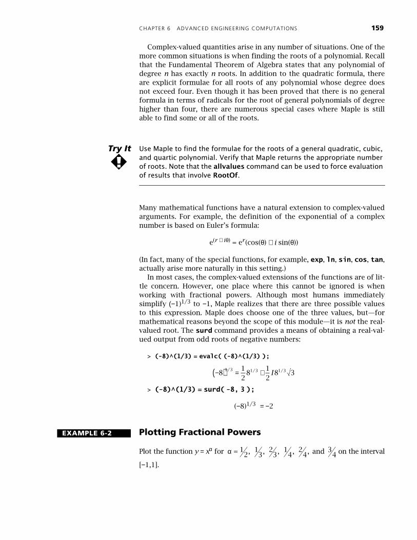
In most cases, the complex-valued extensions of the functions are of lit-tle concern. However, one place where this cannot be ignored is whenworking with fractional powers. Although most humans immediatelysimplify (−1)1/3 to −1, Maple realizes that there are three possible valuesto this expression. Maple does choose one of the three values, but—formathematical reasons beyond the scope of this module—it is not the real-valued root. The surd command provides a means of obtaining a real-val-ued output from odd roots of negative numbers:

> (-8)^(1/3) = evalc( (-8)^(1/3) );

> (-8)^(1/3) = surd( -8, 3 );

(−8)1/3 = −2

Plotting Fractional Powers

Plot the function y = xα for on the interval

[−1,1].

Try It

!

−( ) = +812

812

8 31 3 1 3 1 3/ / /I

EXAMPLE 6-2

α = 1

2, 13, 2

3, 14, 2

4, and 34


SOLUTION

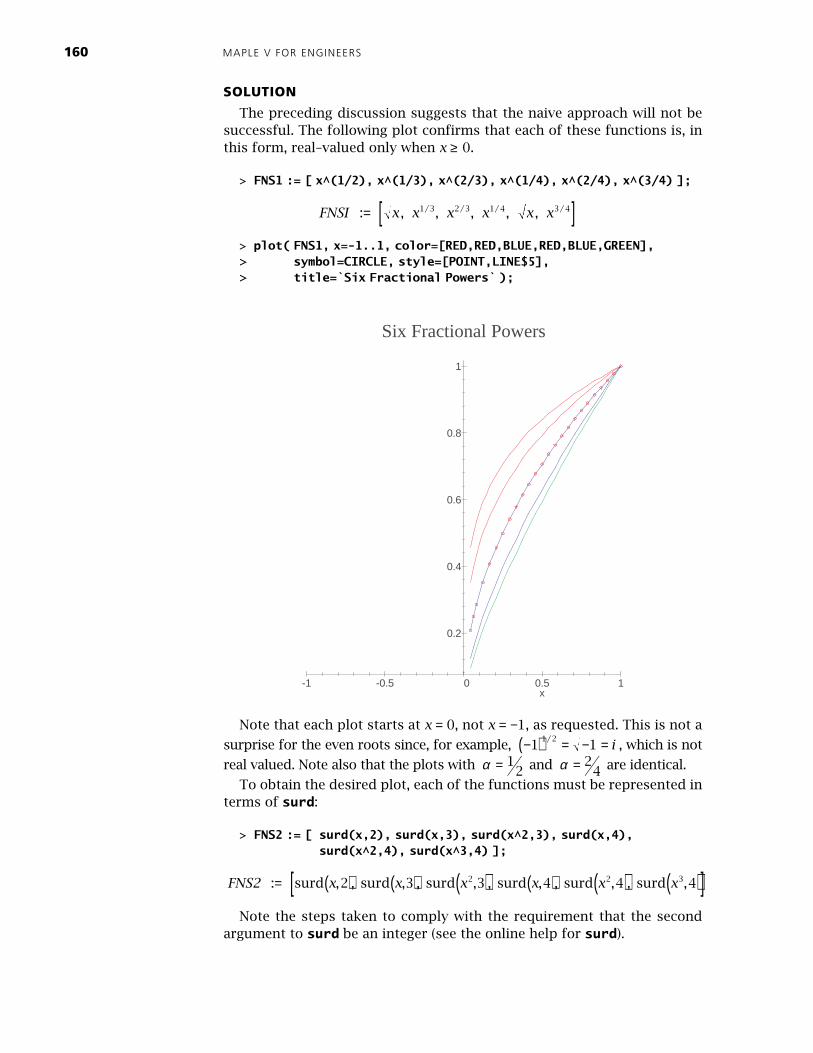
The preceding discussion suggests that the naive approach will not besuccessful. The following plot confirms that each of these functions is, inthis form, real–valued only when x ≥ 0.

> FNS1 := [ x^(1/2), x^(1/3), x^(2/3), x^(1/4), x^(2/4), x^(3/4) ];

> plot( FNS1, x=-1..1, color=[RED,RED,BLUE,RED,BLUE,GREEN],> symbol=CIRCLE, style=[POINT,LINE$5],> title=`Six Fractional Powers` );

Note that each plot starts at x = 0, not x = −1, as requested. This is not a

surprise for the even roots since, for example, , which is not

real valued. Note also that the plots with and are identical.

To obtain the desired plot, each of the functions must be represented interms of surd:

> FNS2 := [ surd(x,2), surd(x,3), surd(x^2,3), surd(x,4),surd(x^2,4), surd(x^3,4) ];

Note the steps taken to comply with the requirement that the secondargument to surd be an integer (see the online help for surd).

FNSI x x x x x x : , , , , , / / / /= [ ]1 3 2 3 1 4 3 4

x10.50-0.5-1

1

0.8

0.6

0.4

0.2

Six Fractional Powers

−( ) = − =1 11 2/

i

α = 12 α = 2

4

FNS2 x x x x x x : surd , , surd , , surd , , surd , , surd , , surd ,= ( ) ( ) ( ) ( ) ( ) ( )[ ]2 3 3 4 4 42 2 3


> plot( FNS2, x=-1..1, color=[RED,RED,BLUE,RED,BLUE,GREEN],> symbol=CIRCLE, style=[POINT,LINE$5],> title=`Six Fractional Powers -- using surd` );

From the second plot, you can see that using surd allowed three of the

plots to be extended to the negative real line.

Identify the three functions that were able to be extended to the negative real line in the final plot in Example 6-2.

Use convert and simplify (and, if necessary, assume) to verify that the surd-based representations are equivalent to the original power represen-

tation. (Pay particular attention to .)

To conclude this brief introduction to complex analysis, it should be men-tioned that the plots package contains commands for creating 2D and 3Dplots of complex-valued functions: complexplot and complexplot3d.

x10.5-0.5-1

1

0.5

0

-0.5

-1

Six Fractional Powers -- using surd

Try It

!

Try It

!α = 2

4


Complex–Valued Solutions of an Equation

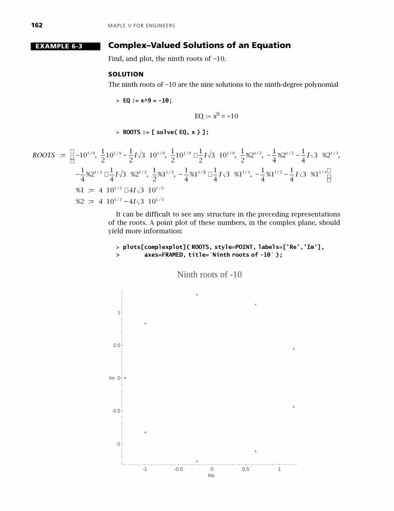
Find, and plot, the ninth roots of −10.

SOLUTION

The ninth roots of −10 are the nine solutions to the ninth-degree polynomial

> EQ := x^9 = -10;

EQ := x9 = −10

> ROOTS := [ solve( EQ, x ) ];

It can be difficult to see any structure in the preceding representationsof the roots. A point plot of these numbers, in the complex plane, shouldyield more information:

> plots[complexplot]( ROOTS, style=POINT, labels=['Re','Im'],> axes=FRAMED, title=`Ninth roots of -10` );

EXAMPLE 6-3

I% % , % , %/ / / /− + −4

24

3 22

14

11 3 1 3 1 3 1 33 1 3 1 3 1 3

1 3 1 3

43 1

41

43 1

1 4 10 4 3 10

+ − −

I I

I

% , % %

%

/ / /

/ /

ROOTS I I I

I

: , , , % , % % ,

% % , % , %

/ / / / / / / /

/ / / /

= − − + − −

− + −

1012

1012

3 1012

1012

3 1012

214

214

3 2

14

214

3 212

114

1

1 9 1 9 1 9 1 9 1 9 1 3 1 3 1 3

1 3 1 3 1 3 1 33 1 3 1 3 1 3

1 3 1 3

1 3 1 3

14

3 114

114

3 1

1 4 10 4 3 10

2 4 10 4 3 10

+ − −

= +

= −

I I

I

I

% , % %

% :

% :

/ / /

/ /

/ /

10.50-0.5-1

Im

1

0.5

0

-0.5

-1

Ninth roots of -10

Re


Note that there is only one real-valued root, and none of the roots arepurely complex. Moreover, the roots appear to be regularly spaced on the

circle centered at the origin with radius a little larger than 1.25.

NODAL ANALYSIS OF AN ELECTRICAL CIRCUIT

Electrical engineers have, as one of their tasks, the analysis and synthe-sis of a variety of circuits. In this application, you will use Maple to con-duct an analysis of a low-pass (LP) electrical filter. An ideal LP filtertransmits an input electrical signal to the output with no attenuationand no phase shift. However, above some cutoff frequency, ωc , the elec-trical signal is completely blocked and usually undergoes some phaseshift as well. The cutoff frequency can be controlled by the properchoice of component values.

No practical filter behaves in such an ideal fashion, but this situationcan be approximated as closely as cost and need dictate. Your analysisof a passive low-pass filter consisting of two inductors and one capaci-tor will show that this filter exhibits resonant (sharp peak) behavior inthe vicinity of the cut-off frequency, which detracts from the ideal uni-form behavior. Nevertheless, its rejection of frequencies beyond thecutoff frequency is a factor of 100 higher than for a simpler (one induc-tor or one capacitor) circuit. Stated in terms of decibels, this improve-ment by a factor of 100 corresponds to 20 log10 (100) = 40 decibels(dB). In practice, an LP filter would likely be constructed from resistors(modeling loss of power) and active circuit elements such as opera-tional amplifiers.

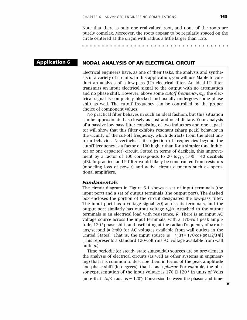
FundamentalsThe circuit diagram in Figure 6-1 shows a set of input terminals (theinput port) and a set of output terminals (the output port). The dashedbox encloses the portion of the circuit designated the low-pass filter.The input port has a voltage signal vi(t) across its terminals, and theoutput port similarly has output voltage vo(t). Attached to the outputterminals is an electrical load with resistance, R. There is an input ACvoltage source across the input terminals, with a 170-volt peak ampli-tude, 120 ° phase shift, and oscillating at the radian frequency of ω radi-ans/second (= 2π60 for AC voltages available from wall outlets in theUnited States). That is, the input source is .(This represents a standard 120-volt rms AC voltage available from walloutlets.)

Time-periodic (or steady-state sinusoidal) sources are so prevalent inthe analysis of electrical circuits (as well as other systems in engineer-ing) that it is common to describe them in terms of the peak amplitudeand phase shift (in degrees), that is, as a phasor. For example, the pha-sor representation of the input voltage is 170 ∠ 120 °, in units of Volts

(note that radians = 120°). Conversion between the phasor and time-

Application 6

v t ti ( ) cos= +( )170 2 3ω π

2 3π

164


periodic representations is based on Euler’s formula, ,

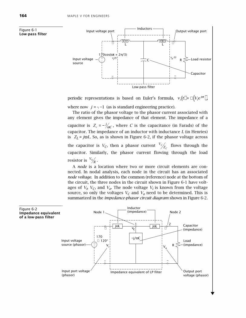
where now (as is standard engineering practice).The ratio of the phasor voltage to the phasor current associated with

any element gives the impedance of that element. The impedance of a

capacitor is , where

C

is the capacitance (in Farads) of the

capacitor. The impedance of an inductor with inductance

L

(in Henries)

is

Z

L

=

j

ω

L

. So, as is shown in Figure 6-2, if the phasor voltage across

the capacitor is

V

C

, then a phasor current flows through the

capacitor. Similarly, the phasor current flowing through the load

resistor is .

A

node

is a location where two or more circuit elements are con-nected. In nodal analysis, each node in the circuit has an associated

node voltage

. In addition to the common (reference) node at the bottom ofthe circuit, the three nodes in the circuit shown in Figure 6-1 have volt-ages of

V

i

,

V

C

, and

V

o

. The node voltage

V

i

is known from the voltagesource, so only the voltages

V

C

and

V

o

need to be determined. This issummarized in the

impedance-phasor circuit diagram

shown in Figure 6-2.

Figure 6-1

Low-pass filter

C R

L L

+

+ +

− −

170cos(ωt + 2π/3)vi(t)

vo (t)

Low-pass filter

Capacitor

Load resistor

Output voltage portInductors

Input voltage port

Input voltage source

−

v t Vi ij t( ) = ℜ( )e ω

j = −1

Zcj

C= − ω

VZ

C

C

VR

0

Figure 6-2

Impedance equivalentof a low-pass filter

R+

+ +

− −

170 ∠ 120°

Vi

vc

Vo

Impedance equivalent of LP filter

Load(impedance)

Node 2Node 1

Input voltage source (phasor)

Capacitor(impedance)

−j/ωC

1 2jωL jωL

Output portvoltage (phasor)

Input port voltage(phasor)

−

Inductor(impedance)


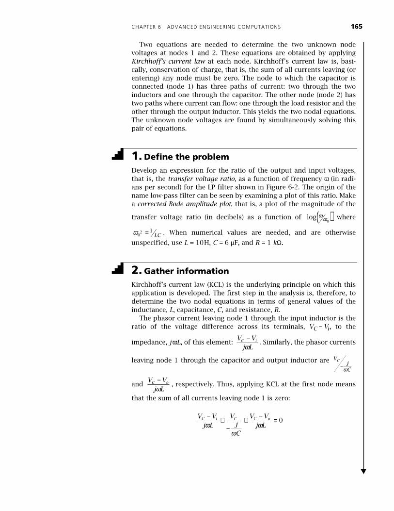
Two equations are needed to determine the two unknown nodevoltages at nodes 1 and 2. These equations are obtained by applyingKirchhoff’s current law at each node. Kirchhoff’s current law is, basi-cally, conservation of charge, that is, the sum of all currents leaving (orentering) any node must be zero. The node to which the capacitor isconnected (node 1) has three paths of current: two through the twoinductors and one through the capacitor. The other node (node 2) hastwo paths where current can flow: one through the load resistor and theother through the output inductor. This yields the two nodal equations.The unknown node voltages are found by simultaneously solving thispair of equations.

1. Define the problem

Develop an expression for the ratio of the output and input voltages,that is, the transfer voltage ratio, as a function of frequency ω (in radi-ans per second) for the LP filter shown in Figure 6-2. The origin of thename low-pass filter can be seen by examining a plot of this ratio. Makea corrected Bode amplitude plot, that is, a plot of the magnitude of the

transfer voltage ratio (in decibels) as a function of where

. When numerical values are needed, and are otherwise

unspecified, use L = 10H, C = 6 µF, and R = 1 kΩ.

2. Gather information

Kirchhoff’s current law (KCL) is the underlying principle on which thisapplication is developed. The first step in the analysis is, therefore, todetermine the two nodal equations in terms of general values of theinductance, L, capacitance, C, and resistance, R.

The phasor current leaving node 1 through the input inductor is theratio of the voltage difference across its terminals, VC − Vi , to the

impedance, j ωL, of this element: . Similarly, the phasor currents

leaving node 1 through the capacitor and output inductor are

and , respectively. Thus, applying KCL at the first node means

that the sum of all currents leaving node 1 is zero:

log ωω0( )

ω02 = 1

LC

V Vj L

C i−ω

VjC

C

−ω

V Vj L

C o−ω

V Vj L

VjC

V Vj L

C i C C o− +−

+ − =ω

ωω

0


The second node connects only two elements. The current phasorleaving the output inductor is the negative of the current entering that

element: ; the current phasor through the resistor is . The

equation obtained from applying KCL at node 2 is

3. Generate and evaluate potential solutions

In order to be faithful to engineering notation, it is preferable to over-ride Maple’s use of I to represent . The online help for I tells youthat I is simply an alias for . Then, following the hyperlink to thehelp worksheet for alias, you quickly learn that the following com-mand both removes the alias for I and adds a new alias for j.

> restart;> alias( I=I, j = sqrt(-1) );

j

The equations representing KCL at the two nodes are

> EQ1 := (V[C]-V[i])/j/omega/L + V[C]/(-j/omega/C) +> (V[C]-V[o])/j/omega/L = 0;

> EQ2 := (V[o]-V[C])/(j*omega*L) + V[o]/R = 0;

The voltage transfer ratio as a function of frequency (or, simply, thefrequency response) for this circuit is the ratio of the output and input

voltage phasors: . This expression is easily constructed once VC and

Vo are known.

> SOLN := solve( EQ1, EQ2 , V[C], V[o] );

V Vj L

o C−ω

V

R0

V V

j L

V

Ro C− + =

ω0 0

−1−1

EQ1j V V

LjV C

j V V

LC i

CC : = −

−( )+ −

−( )=

ωω

ω0 0

EQ2j V V

LVR

o C : = −−( )

+ =ω

0 0

VV

o

i

SOLN VV jR L

jR jR CL L L CV

jRV

jR jR CL L L CC

i

oi : , = = −

−( )− + + −

= −− + + −

ω

ω ω ω ω ω ω2 3 2 2 3 22 2


Although these solutions are complicated functions of frequency, itis not difficult to see that these voltages respond linearly to a change inthe input voltage. The ratio of the output and input voltages is, there-fore, independent of the input voltage, Vi :

> RESPONSE := subs( SOLN, V[o]/V[i] );

Note that the frequency response is, for most frequencies, a complex

number. If it is written in polar form, = M e j θ, the magnitude M is

commonly called the gain, and θ is called the relative phase shift (relativeto the phase of the input source). The gain is found to be

> M := evalc( abs( RESPONSE ) );

which can be simplified, with normal (because of the rational functionsthat appear in M) and collect (to show the structure relative to ω) tothe somewhat more manageable form

> M := map( collect, normal( M ), omega );

(The map command is needed to force the collection with respect to ωin the numerator and denominator of this expression. Compare thisresult with that obtained from collect( normal( M ), omega );.)

The phase angle is the argument of a complex-valued frequencyresponse function. Maple’s argument is used in the same manner asabs, Re, and Im:

> theta := argument( RESPONSE );

The argument is, essentially, the arctangent of the ratio of the imagi-nary and real parts of the expression. (Exceptions occur when the realpart is zero; furthermore, the signs of the real and imaginary partsmust be used to determine the correct quadrant for the argument; seethe online help for argument and invtrig for further details.)

RESPONSEjR

jR jR CL L L C : =

− + + −ω ω ω2 3 22

VV

o

i

MR L L C

L L C R R CL

R R R CL

L L C R R CL : =

−( )−( ) + − +( )

+− +( )

−( ) + − +( )

2 3 2 2

3 2 2 2 2 2

2 2 2

3 2 2 2 2 2

2

2 2

ω ω

ω ω ω

ω

ω ω ω

MR

L C L C R C L L R CL R : =

+ − +( ) + −( ) +

2

6 4 2 3 2 2 2 4 2 2 2 24 4 2ω ω ω

θω ω ω

: argument=− + + −

jR

jR jR CL L L C2 3 22


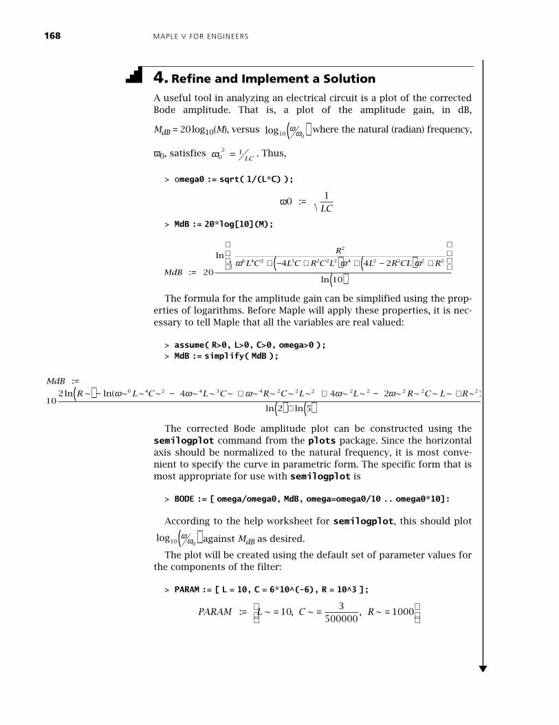
4. Refine and Implement a Solution

A useful tool in analyzing an electrical circuit is a plot of the correctedBode amplitude. That is, a plot of the amplitude gain, in dB,

MdB = 20log10(M), versus where the natural (radian) frequency,

ω0, satisfies . Thus,

> omega0 := sqrt( 1/(L*C) );

> MdB := 20*log[10](M);

The formula for the amplitude gain can be simplified using the prop-erties of logarithms. Before Maple will apply these properties, it is nec-essary to tell Maple that all the variables are real valued:

> assume( R>0, L>0, C>0, omega>0 );> MdB := simplify( MdB );

The corrected Bode amplitude plot can be constructed using thesemilogplot command from the plots package. Since the horizontalaxis should be normalized to the natural frequency, it is most conve-nient to specify the curve in parametric form. The specific form that ismost appropriate for use with semilogplot is

> BODE := [ omega/omega0, MdB, omega=omega0/10 .. omega0*10]:

According to the help worksheet for semilogplot, this should plot

against MdB as desired.

The plot will be created using the default set of parameter values forthe components of the filter:

> PARAM := [ L = 10, C = 6*10^(-6), R = 10^3 ];

log10 0ω

ω( )ω0

2 1=LC

ω01

: =LC

MdB

R

L C L C R C L L R CL R :

ln

ln=

+ − +( ) + −( ) +

( )204 4 2

10

2

6 4 2 3 2 2 2 4 2 2 2 2ω ω ω

MdB

R L C L C R C L L R C L R

:

ln ~ ln( ~ ~ ~ ~ ~ ~ ~ ~ ~ ~ ~ ~ ~ ~ ~ ~ ~ )

ln ln

=

( ) − − + + − +

( ) + ( )102 4 4 2

2 5

6 4 2 4 3 4 2 2 2 2 2 2 2 2ω ω ω ω ω

log10 0ω

ω( )

PARAM L C R : ~ , ~ , ~= = = =

103

5000001000

CHAPTER 6 ADVANCED ENGINEERING COMPUTATIONS

169

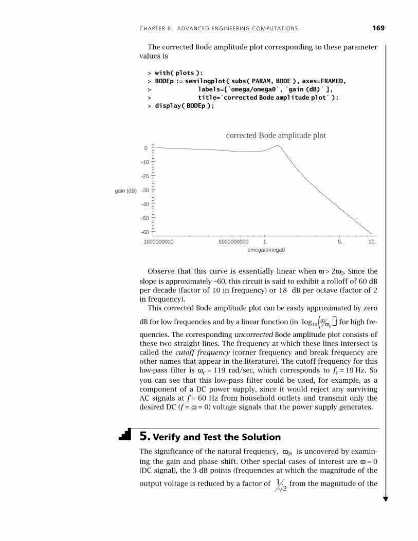
The corrected Bode amplitude plot corresponding to these parametervalues is

>

with(

plots

):

>

BODEp

:=

semilogplot(

subs(

PARAM,

BODE

),

axes=FRAMED,

>

labels=[`omega/omega0`,

`gain

(dB)`

],

>

title=`corrected

Bode

amplitude

plot`

):

>

display(

BODEp

);

Observe that this curve is essentially linear when

ω

> 2

ω

0

. Since the

slope is approximately

−

60, this circuit is said to exhibit a rolloff of 60 dBper decade (factor of 10 in frequency) or 18 dB per octave (factor of 2in frequency).

This corrected Bode amplitude plot can be easily approximated by zero

dB for low frequencies and by a linear function (in ) for high fre-

quencies. The corresponding

uncorrected

Bode amplitude plot consists ofthese two straight lines. The frequency at which these lines intersect iscalled the

cutoff frequency

(corner frequency and break frequency areother names that appear in the literature). The cutoff frequency for thislow-pass filter is

ω

c

= 119 rad/sec, which corresponds to

f

c

=

19 Hz. So

you can see that this low-pass filter could be used, for example, as acomponent of a DC power supply, since it would reject any survivingAC signals at

f

= 60 Hz from household outlets and transmit only thedesired DC (

f

=

ω

= 0) voltage signals that the power supply generates.

5.

Verify and Test the Solution

The significance of the natural frequency,

ω

0

, is uncovered by examin-

ing the gain and phase shift. Other special cases of interest are

ω

= 0(DC signal), the 3 dB points (frequencies at which the magnitude of the

output voltage is reduced by a factor of from the magnitude of the

omega/omega0

10.5.1..5000000000.1000000000

gain (dB)

0

-10

-20

-30

-40

-50

-60

corrected Bode amplitude plot

log10 0ω

ω( )

12


input source), and the asymptotic behavior for large frequencies (seeProblem 9). The consideration of each of these special cases both addsto our understanding of this problem and confirms the utility of thegeneral expressions obtained in Step 4.

Special Case 1: Direct Current (ω = 0)

The frequency of a DC source is ω = 0 so the impedance is zero for eachinductor and is infinite for the capacitor. Thus, referring to Figure 6-2,the low-pass filter is seen to simply transmit the input unchangedthrough to the output port since the inductors become short-circuitedwires and the capacitor becomes an open-circuit at DC. Thus, this filtershould exhibit a gain of 1 and no phase shift.

Recall that the gain and phase shift are, in general, given by

> M;

> theta;

In this case it is clear that the gain is M = 1 and the phase shift isθ = arctan(0) = 0. The same results are obtained by Maple:

> gain = simplify( subs( omega=0, M ) );

gain = 1

> phaseshift = simplify( subs( omega=0, theta ) );

phaseshift = 0

Special Case 2: Natural Frequency (ω = ω0 )

The natural frequency of the circuit occurs when ω = ω0 . The gain andphase shift in this case are

> gain = simplify( subs( omega=omega0, M ) );

> phaseshift = simplify( subs( omega=omega0, theta ) );

Observe that though the gain of a low-pass filter at the natural fre-quency depends on the specific values of the circuit parameters, thephase shift is always −90 °.

R

L C L C R C L L R CL R

2

6 4 2 3 2 2 2 4 2 2 2 24 4 2ω ω ω+ − +( ) + −( ) +

argument −− + + −

jRjR jR CL L L Cω ω ω2 3 22

gain RCL

= ~~~

phaseshift = − 12

π


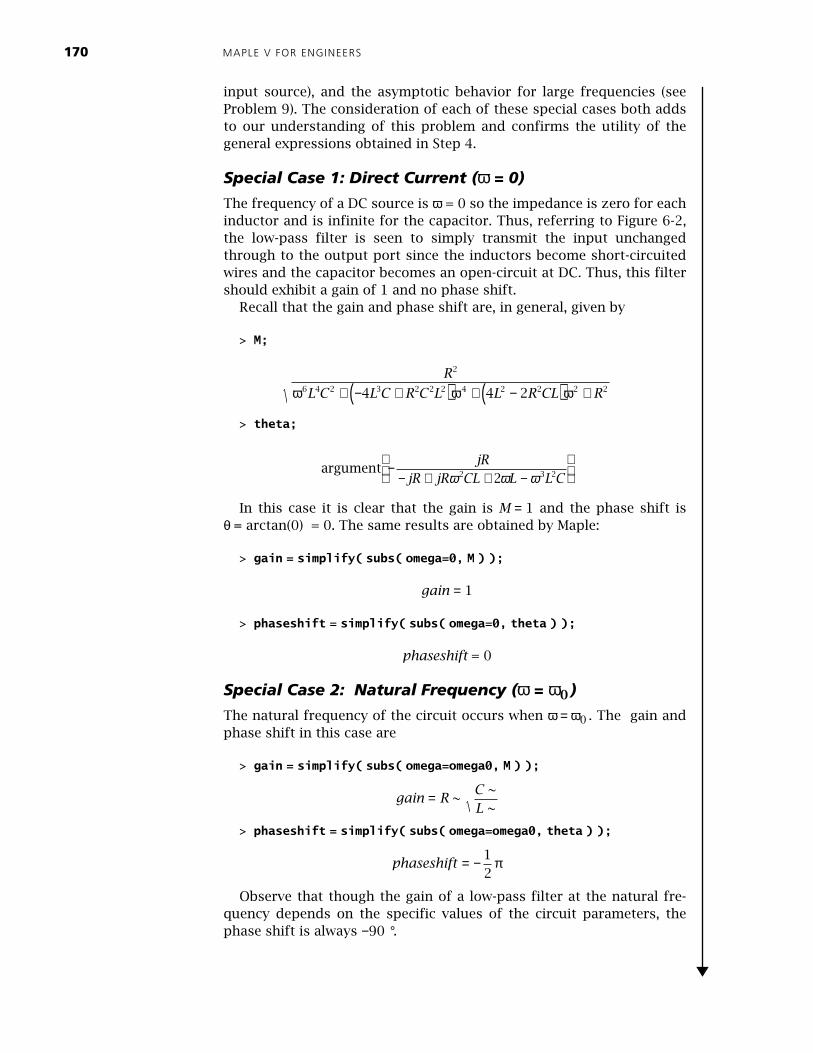
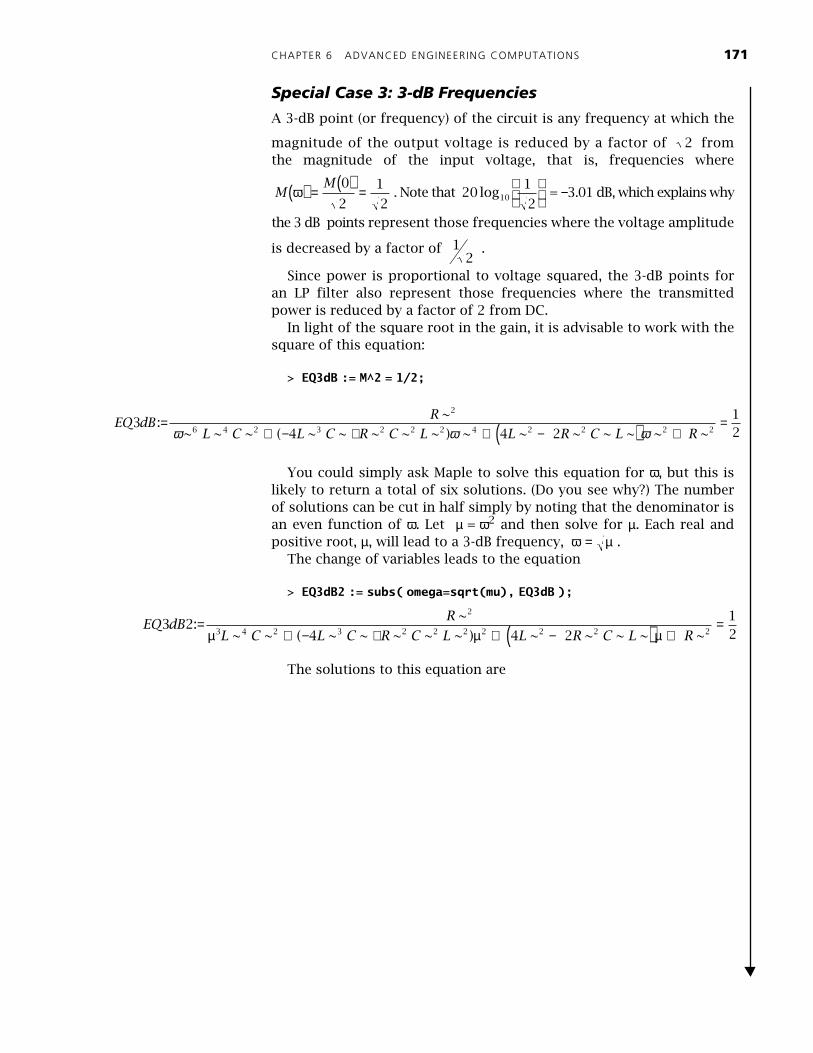
Special Case 3: 3-dB Frequencies

A 3-dB point (or frequency) of the circuit is any frequency at which the

magnitude of the output voltage is reduced by a factor of fromthe magnitude of the input voltage, that is, frequencies where

. Note that = −3.01 dB, which explains why

the 3 dB points represent those frequencies where the voltage amplitude

is decreased by a factor of .

Since power is proportional to voltage squared, the 3-dB points foran LP filter also represent those frequencies where the transmittedpower is reduced by a factor of 2 from DC.

In light of the square root in the gain, it is advisable to work with thesquare of this equation:

> EQ3dB := M^2 = 1/2;

You could simply ask Maple to solve this equation for ω, but this islikely to return a total of six solutions. (Do you see why?) The numberof solutions can be cut in half simply by noting that the denominator isan even function of ω. Let µ = ω2 and then solve for µ. Each real andpositive root, µ, will lead to a 3-dB frequency, .

The change of variables leads to the equation

> EQ3dB2 := subs( omega=sqrt(mu), EQ3dB );

The solutions to this equation are

2

MM

ω( ) = ( ) =0

2

1

220

1

210log

12

EQ dBR

L C L C R C L L R C L R3

4 4 2

12

2

6 4 2 3 2 2 2 4 2 2 2 2:

~

~ ~ ~ ( ~ ~ ~ ~ ~ ) ~ ~ ~ ~ ~ ~ ~=

+ − + + −( ) +=

ω ω ω

ω µ=

EQ dBR

L C L C R C L L R C L R3 2

4 4 2

12

2

3 4 2 3 2 2 2 2 2 2 2:

~

~ ~ ( ~ ~ ~ ~ ~ ) ~ ~ ~ ~ ~=

+ − + + −( ) +=

µ µ µ


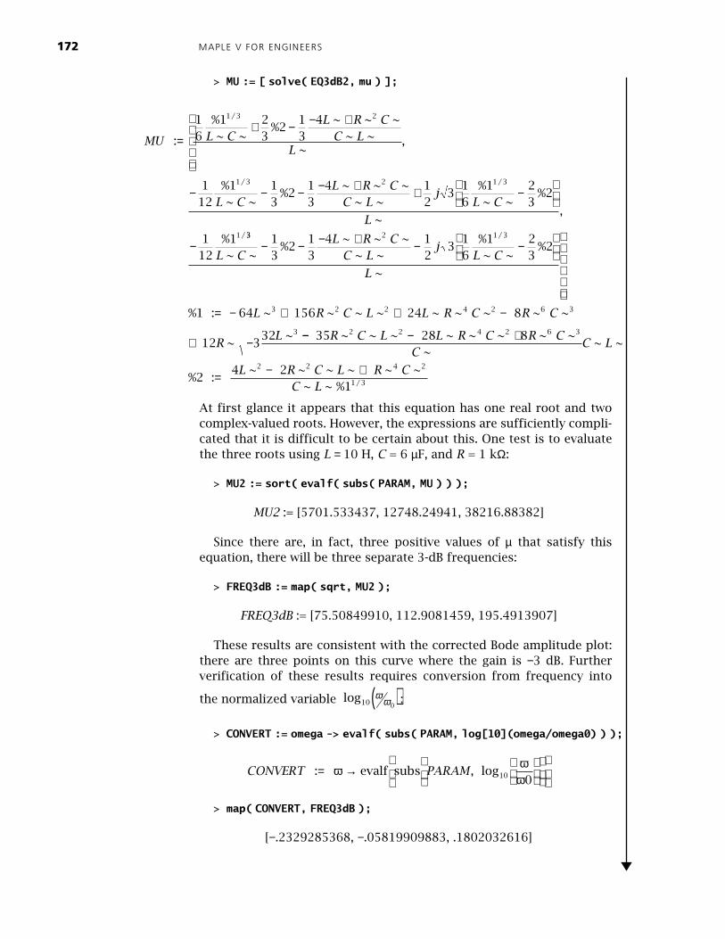
> MU := [ solve( EQ3dB2, mu ) ];

At first glance it appears that this equation has one real root and twocomplex-valued roots. However, the expressions are sufficiently compli-cated that it is difficult to be certain about this. One test is to evaluatethe three roots using L = 10 H, C = 6 µF, and R = 1 kΩ:

> MU2 := sort( evalf( subs( PARAM, MU ) ) );

MU2 := [5701.533437, 12748.24941, 38216.88382]

Since there are, in fact, three positive values of µ that satisfy thisequation, there will be three separate 3-dB frequencies:

> FREQ3dB := map( sqrt, MU2 );

FREQ3dB := [75.50849910, 112.9081459, 195.4913907]

These results are consistent with the corrected Bode amplitude plot:there are three points on this curve where the gain is −3 dB. Furtherverification of these results requires conversion from frequency into

the normalized variable :

> CONVERT := omega -> evalf( subs( PARAM, log[10](omega/omega0) ) );

> map( CONVERT, FREQ3dB );

[−.2329285368, −.05819909883, .1802032616]

MU L CL R C

C LL

L CL R C

C Lj

L C

L

:

%~ ~

%~ ~ ~

~ ~~

,

%~ ~

%~ ~ ~

~ ~%~ ~

%

~,

%

/

/ /

/

=+ − − +

− − − − + + −

−

16

1 23

213

4

112

1 13

213

4 12

316

1 23

2

112

1

1 3 2

1 3 2 1 3

1 33 2 1 3

3 2 2 4 2 6 3

3

13

213

4 12

316

1 23

2

1 64 156 24 8

12 332

L CL R C

C Lj

L C

L

L R C L L R C R C

RL

~ ~%

~ ~ ~~ ~

%~ ~

%

~

% : ~ ~ ~ ~ ~ ~ ~ ~ ~

~~

/

− − − + − −

= − + + −

+ − −− − +

= − +

~ ~ ~ ~ ~ ~ ~ ~~

~ ~

% : ~ ~ ~ ~ ~ ~

~ ~ % /

35 28 8

24 2

1

2 2 4 2 6 3

2 2 4 2

1 3

R C L L R C R CC

C L

L R C L R CC L

log10 0ω

ω( )

CONVERT PARAM : evalf subs , log= →

ω ω

ω10 0


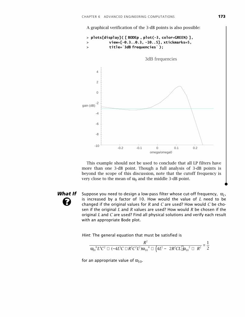
A graphical verification of the 3-dB points is also possible:

> plots[display]( [ BODEp , plot(-3, color=GREEN) ],> view=[-0.3..0.3, -10..5], xtickmarks=5,> title=`3dB frequencies` );

This example should not be used to conclude that all LP filters havemore than one 3-dB point. Though a full analysis of 3-dB points isbeyond the scope of this discussion, note that the cutoff frequency isvery close to the mean of ω0 and the middle 3-dB point.

Suppose you need to design a low-pass filter whose cut-off frequency, ωc,is increased by a factor of 10. How would the value of L need to bechanged if the original values for R and C are used? How would C be cho-sen if the original L and R values are used? How would R be chosen if theoriginal L and C are used? Find all physical solutions and verify each resultwith an appropriate Bode plot.

Hint: The general equation that must be satisfied is

for an appropriate value of ω10.

omega/omega00.20.10-0.1-0.2

gain (dB)

4

2

0

-2

-4

-6

-8

-10

3dB frequencies

What If

?

R

L C L C R C L L R CL R

2

106 4 2 3 2 2 2

104 2 2

102 24 4 2

12ω ω ω+ − + + −( ) +

= ( )


6-2 CALCULUSLimits are the fundamental concept behind the two principal componentsof calculus: the derivative and the integral. The corresponding Maple com-mands are limit, diff, and int and their inert forms Limit, Diff, andInt. This brief introduction discusses only these fundamental concepts;the student package contains a large collection of additional calculus-basedtools, including integration by parts, line integrals, and triple integrals.

The limit of an expression f(x) as x approaches a, , is translated

to Maple as limit( f(x), x=a ); . An optional third argument can be usedto specify one-sided limits.

Limits

Use Maple to evaluate each of the following limits:

(a)

(b)

(c)

(d)

(e)

(f)

SOLUTION

Each limit can be directly translated into Maple. The only special consider-ation is in (c), where the one-sided limit from the left is specified byincluding left as the third argument of the limit command

> restart;

(a) > limit( (x^3+8)/(x+2), x=-2 );

12

(b) > limit( tan(theta/2), theta=Pi );

undefined

(c) > limit( tan(theta/2), theta=Pi, left );

∞

lim fx a

x→

( )

EXAMPLE 6-4

limx

xx→ −

++2

3 82

lim tanθ π

θ→

2

lim tanθ π

θ→ −

2

limsin

x

x

x x→

−( )− + +3

2

3 2

3 27

2 45

lim sinx x→

0

1

limsin sin

y x

y x

y x→

( ) − ( )−


(d) > limit( sin(3*x^2-27)/(x^2-2*x^3+45), x=3 );

(e) > limit( sin(1/x), x=0 );

−1 .. 1

(f) > limit( (sin(y)-sin(x))/(y-x), y=x );

cos(x)

The results from parts (b) and (c) illustrate the way Maple responds tolimits that do not exist or are unbounded. The result in (e) should be inter-

preted to mean that the limit is not defined because the value of

oscillates within the interval [−1,1] infinitely often near x = 0. The limit in(f) is recognized as the definition of the derivative of sin(x); in light of this

observation, the result is exactly what you should expect.

The Limit command is the inert, or unevaluated, form of limit. Exceptthat the inert form of a function is not evaluated, it is identical to the reg-ular form of the command. Two common usages of the inert form of acommand are to verify that the correct quantity has been entered and tohave more control over the evaluation of the expression. The value com-mand forces evaluation of the inert form with the corresponding normalversion of the command (for example, replace Limit with limit and thencall value); the evalf command can be used if a purely numeric evalua-tion is desired.

Euler’s constant, e

Euler’s constant, e, can be defined as . Use the inert form

of limit to evaluate this limit both symbolically and numerically using20 significant digits.

SOLUTION

The definition of e, as an unevaluated limit, is

> eLIM := Limit( (1+1/n)^n, n=infinity );

eLIM :=

The normal evaluation of this inert expression is forced using thevalue command.

> eLIM = value( eLIM );

= e

−38

sin1x

EXAMPLE 6-5

limn

n

n→∞+( )1 1

limn

n

n→∞+

11

limn

n

n→∞+

11


The floating-point evaluation of the same limit, using 20 digits in thecomputations, can be obtained using evalf:

> eLIM = evalf( eLIM, 20 );

= 2.7182818284590452354

Note how the presentation of the limit and its value in Example 6-5 is more informative than the format used in Example 6-4. Redo each of the problems in Example 6-4 using a style similar to that introduced inExample 6-5.

Asymptotes of a Rational Function

Find all asymptotes (vertical, horizontal, and oblique) for the function

. Create a plot that clearly shows all interesting features

of f.

SOLUTION

The function could be entered as a Maple expression or, using the arrowoperator, as a function. For a change of pace, and in preparation of laterexamples in this chapter, the arrow operator will be used here:

> f := x -> (2*x^2-7*x+1)/(3-x);

The singularity in the denominator when x = 3 suggests the probableexistence of a vertical asymptote at x = 3. To confirm this, it is necessaryto check that at least one of the left and right one-sided limits isunbounded at x = 3:

> limR := Limit( f(x), x=3, right ):> limR = value( limR );

> limL := Limit( f(x), x=3, left ):> limL = value( limL );

Thus, x = 3 is a vertical asymptote for f.

limn

n

n→∞+

11

Try It

!

EXAMPLE 6-6

f xx x

x( ) = − +

−2 7 1

3

2

f xx x

x:= → − +

−2 7 1

3

2

x

x xx→ +

− +−

= ∞3

22 7 13

lim

x

x xx→ −

− +−

= −∞3

22 7 13

lim


Since the degree of the numerator exceeds the degree of the denominator,there are no horizontal asymptotes to this function. But there should bean oblique asymptote. Long division is the usual technique used to manu-ally compute an oblique asymptote. The Maple commands quo and remcan be used to obtain this information. The oblique asymptote can be ob-tained from the quotient of the numerator and denominator of f as follows:

> NN := numer( f(x) );> DD := denom( f(x) );

NN := −2x2 + 7x − 1DD := −3 + x

> obliq_asymp := quo( NN, DD, x, 'rest' );

obliq_asymp := −2x + 1

Observe how the optional fourth argument to quo is used to obtainboth the remainder and quotient simultaneously. Thus, an equivalent rep-resentation of the function should be

> fEQUIV := obliq_asymp + rest/DD;

One way to check this result is to normalize the difference between thetwo representations of the function:

> simplify( fEQUIV - f(x) );

0

Since this difference is zero, the two representations are equivalent.All that remains is to verify that y = −2x + 1 is an oblique asymptote for f:> obliqLIM1 := Limit( f(x)-obliq_asymp, x=infinity ):> obliqLIM1 = value( obliqLIM1 );

> obliqLIM2 := Limit( f(x)-obliq_asymp, x=-infinity ):> obliqLIM2 = value( obliqLIM1 );

Of course, these results can be seen by inspection from the fact that

. (Three alternative methods for finding the oblique

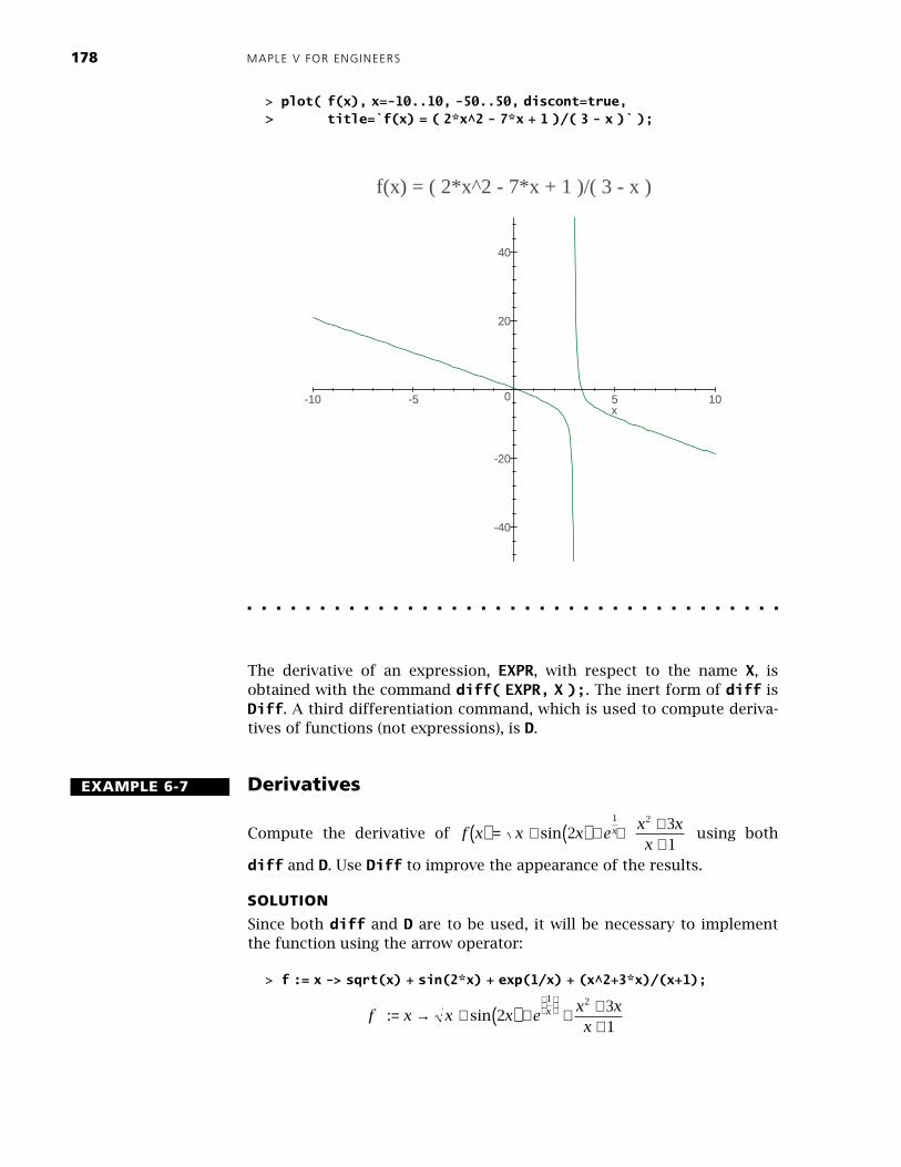
asymptote are presented in Problem 3 in this chapter.)The last step is to create a plot of the function f. Since f is discontinu-

ous, you know that it is necessary to use the discont=true option and toprovide an appropriate vertical range:

fEQUIV xx

: = − + +− +

2 12

3

x

x xx

x→∞

− +−

+ − =lim2 7 1

32 1 0

2

x

x xx

x→ −∞( )

− +−

+ − =lim2 7 1

32 1 0

2

f x xx

( ) − − +( ) =−

2 12

3


> plot( f(x), x=-10..10, -50..50, discont=true,> title=`f(x) = ( 2*x^2 - 7*x + 1 )/( 3 - x )` );

The derivative of an expression, EXPR, with respect to the name X, isobtained with the command diff( EXPR, X );. The inert form of diff isDiff. A third differentiation command, which is used to compute deriva-tives of functions (not expressions), is D.

Derivatives

Compute the derivative of using both

diff and D. Use Diff to improve the appearance of the results.

SOLUTION

Since both diff and D are to be used, it will be necessary to implementthe function using the arrow operator:

> f := x -> sqrt(x) + sin(2*x) + exp(1/x) + (x^2+3*x)/(x+1);

x105-5-10

40

20

0

-20

-40

f(x) = ( 2*x^2 - 7*x + 1 )/( 3 - x )

EXAMPLE 6-7

f x x x ex xx

x( ) = + ( ) + + ++

sin 231

1 2

f x x x ex xx

x : sin= → + ( ) + + ++

2

31

1 2


The unevaluated derivative is obtained using Diff with the expressionf(x); evaluation is forced using the value command.

> df := Diff( f(x), x );

> df = value( df );

To produce the same result using D, it is necessary to first compute thefunction (not expression) that is the derivative of the function f.

> Df := D(f);

Since Df is a function, the value of this function is obtained by supply-ing an argument. Thus, another way to present the derivative is

> df = Df(x);

Note that Maple displays all derivatives using the standard notation forpartial derivatives. This is something that you need to accept; it cannot bechanged.

Second- and higher-order derivatives can be found by specifying addi-tional arguments to diff or Diff. For example, the second and fifth deriv-atives of EXPR with respect to X can be obtained with diff( EXPR, X, X )and diff( EXPR, X $ 5 ), respectively. The corresponding second andfifth derivative functions obtained with D would be D( D( f ) ) and, usingthe repeated composition operator @@, ( D @@ 5 )( f ).

Compute the first three derivatives of the function using both diff and D. (See also Problem 4 in this chapter).

Note the close correspondence between Maple syntax and mathematicalnotation and terminology. This connection is particularly strong for the

dfx

x x ex xx

x : sin= + ( ) + + ++

∂

∂2

31

1 2

∂∂x

x x ex xx x

xex

xx

x x

xx

x

+ ( ) + + ++

= + ( ) − + +

+− +

+( )

sin cos231

12

12 2

2 31

3

1

1 21

2

2

2

Df xx

xex

xx

x x

x

x

: cos= → + ( ) − + ++

− ++( )

1

21

2 22 3

13

1

1

2

2

2

∂∂x

x x ex xx x

xex

xx

x x

xx

x

+ ( ) + + ++

= + ( ) − + +

+− +

+( )

sin cos231

12

12 2

2 31

3

1

1 21

2

2

2

Try It

!f x x( ) =

−e

12


integration commands, int and Int. Example 6-8 provides illustrations ofindefinite integrals. Proper and improper definite integrals are examinedin Example 6-9. Integrals of piecewise-defined functions are discussed inExamples 6-10 and 6-11. The Strength and Toughness application fromChapter 2 is revisited in Examples 6-10 and 6-11. Example 6-12, involvingnumerical integration, illustrates the increased efficiency that can resultfrom the intelligent use of the inert form of a command.

A Trigonometric Integral

Evaluate the indefinite integral for all real numbers b.

SOLUTION

The inert integration command is used here to, once again, improve theclarity of the results.

> indefINT := Int( sin(x)*cos(b*x), x ):> indefINT = value( indefINT );

Observe that Maple does not include the constant of integration. Thus,it is your responsibility to include an appropriate constant of integration,using a name selected by the user, whenever it is needed. This will beillustrated in all subsequent examples.

Note that this result cannot be applied when b = 1 or b = −1. Sincecos(−x) = cos(x), cosine is an even function, and the results for the two spe-cial cases should be the same. The indefinite integrals when b = 1 andb = −1 are found to be

> indefINT1 := subs( b=1, indefINT ):> indefINT1 = value( indefINT1 ) + C;

> indefINT2 := subs( b=-1, indefINT ):> indefINT2 = value( indefINT2 ) + C;

The indefinite integrals when b = 1 are easily found using the substitution u = sin(x). The integrals could also be found by using the substitution

v = cos(x) or by noting that . Compute the indefinite

integral . Does this yield the same result as in Example 6-8?

Are the results equivalent? Explain.

EXAMPLE 6-8

sin cosx bx dx( ) ( )∫

sin coscos cos

x bx dxb x

b

b x

b( ) ( ) = −

+( )( )+

+− +( )( )

− +∫ 12

1

112

1

1

sin cos sinx x dx x C( ) ( ) = ( ) +∫ 12

2

sin cos sinx x dx x C( ) ( ) = ( ) +∫ 12

2

Try It

!sin cos

sinx x

x( ) ( ) = ( )2

2

sin 2

2

xdx

( )∫


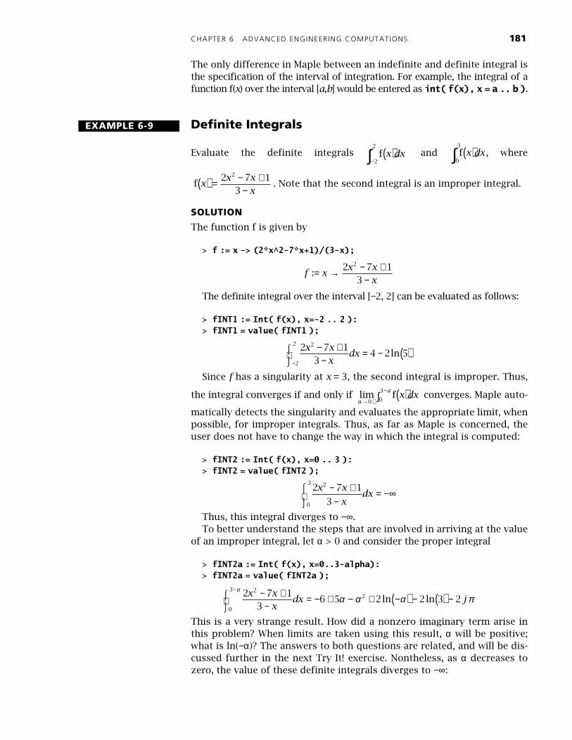
The only difference in Maple between an indefinite and definite integral isthe specification of the interval of integration. For example, the integral of afunction f(x) over the interval [a,b] would be entered as int( f(x), x = a .. b ).

Definite Integrals

Evaluate the definite integrals and , where

. Note that the second integral is an improper integral.

SOLUTION

The function f is given by

> f := x -> (2*x^2-7*x+1)/(3-x);

The definite integral over the interval [−2, 2] can be evaluated as follows:

> fINT1 := Int( f(x), x=-2 .. 2 ):> fINT1 = value( fINT1 );

Since f has a singularity at x = 3, the second integral is improper. Thus,

the integral converges if and only if converges. Maple auto-

matically detects the singularity and evaluates the appropriate limit, whenpossible, for improper integrals. Thus, as far as Maple is concerned, theuser does not have to change the way in which the integral is computed:

> fINT2 := Int( f(x), x=0 .. 3 ):> fINT2 = value( fINT2 );

Thus, this integral diverges to −∞.To better understand the steps that are involved in arriving at the value

of an improper integral, let α > 0 and consider the proper integral

> fINT2a := Int( f(x), x=0..3-alpha):> fINT2a = value( fINT2a );

This is a very strange result. How did a nonzero imaginary term arise inthis problem? When limits are taken using this result, α will be positive;what is ln(−α)? The answers to both questions are related, and will be dis-cussed further in the next Try It! exercise. Nontheless, as α decreases tozero, the value of these definite integrals diverges to −∞:

EXAMPLE 6-9

f x dx( )−∫ 2

2f x dx( )∫0

3

f xx x

x( ) = − +

−2 7 1

3

2

f xx x

x:= → − +

−2 7 1

3

2

2 7 13

4 2 52

2

2 x xx

dx− +−

⌠⌡

= − ( )−

ln

lim fα→ +

− ( )∫0 0

3x dx

a

2 7 1

3

2

0

3x x

xdx

− +−

⌠⌡

= −∞

2 7 13

6 5 2 2 3 22

0

32x x

xdx j

− +−

⌠⌡

= − + − + −( ) − ( ) −−α

α α α πln ln

182


>

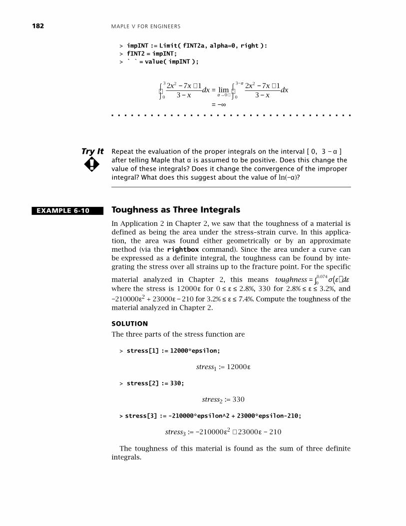
impINT

:=

Limit(

fINT2a,

alpha=0,

right

):

>

fINT2

=

impINT;

>

` `

=

value(

impINT

);

Repeat the evaluation of the proper integrals on the interval [ 0, 3

− α

] after telling Maple that

α

is assumed to be positive. Does this change the value of these integrals? Does it change the convergence of the improper

integral? What does this suggest about the value of

ln(

−α

)

?

Toughness as Three Integrals

In Application 2 in Chapter 2, we saw that the toughness of a material isdefined as being the area under the stress–strain curve. In this applica-tion, the area was found either geometrically or by an approximatemethod (via the

rightbox

command). Since the area under a curve canbe expressed as a definite integral, the toughness can be found by inte-grating the stress over all strains up to the fracture point. For the specific

material analyzed in Chapter 2, this means where the stress is 12000

ε

for 0

≤

ε

≤

2.8%, 330 for 2.8%

≤

ε

≤

3.2%, and

−

210000

ε

2

+ 23000

ε −

210 for 3.2%

≤

ε

≤

7.4%. Compute the toughness of thematerial analyzed in Chapter 2.

SOLUTION

The three parts of the stress function are

>

stress[1]

:=

12000*epsilon;

stress

1

:= 12000

ε

>

stress[2]

:=

330;

stress

2

:= 330

>

stress[3]

:=

-210000*epsilon^2

+

23000*epsilon-210;

stress

3

:=

−

210000

ε

2

+

23000

ε

−

210

The toughness of this material is found as the sum of three definiteintegrals.

2 7 13

2 7 13

2

0

3

0

2

0

3x xx

dxx x

xdx

− +−

⌠⌡

= − +−

⌠⌡

= −∞→ +

−

limα

α

Try It

!

EXAMPLE 6-10

toughness d= ( )∫ σ ε ε0

0 074.


> toughness := Int( stress[1], epsilon=0..0.028 )> + Int( stress[2], epsilon=0.028..0.032 )> + Int( stress[3], epsilon=0.032..0.074 ):> toughness = value( toughness );

To two significant digits, the toughness of this material is 22. Observethat this is well within the range found at the end of Step 3 of the analysis

in Chapter 2.

The specification of the stress–strain curve in three separate parts is anatural part of this problem. This did not impede the determination of thetoughness, but it does complicate the generation of a plot of the stress–strain curve.

The piecewise command can be used to specify, in a single Maple object,all the different pieces of the function. The arguments to piecewise comein pairs of expressions where the first expression in each pair is Boolean(evaluates to either true or false). For example, the piecewise definitionof the stress-strain curve is

> stressPW := piecewise( epsilon<0.028, stress[1],> epsilon<0.032, stress[2],> epsilon<0.074, stress[3] );

Note the convenient printed format—exactly what would be found inany standard mathematical discussion.

If ε has a value, the value returned by piecewise is the expression cor-responding to the first Boolean expression that evaluates to true. (See theonline help worksheet for piecewise for an explanation of the returnvalue when none of the Boolean expressions are true.) Do not despair.This sounds more confusing than it is. To be sure you understand howthis works, consider the following examples:

> eval( subs( epsilon = 0, stressPW ) );

0

> eval( subs( epsilon = 0.01, stressPW ) );

120.00


310.960000

12000 330 210000 23000 210 22 330080000

028

028

0322

032

074

ε ε ε ε ε εd d d.

.

.

.

.

.∫ ∫ ∫+ + − + − =

stressPW :

.

.

.

=<<

− + − <

12000 028

330 032

210000 23000 210 0742

ε εε

ε ε ε



0

The last result is zero because this is the default value returned from apiecewise-defined function when none of the Boolean expressions evalu-ates to true.

Use the piecewise definition of stress and strain to create a plot of the stress-strain curve for the material analyzed in Chapter 2.

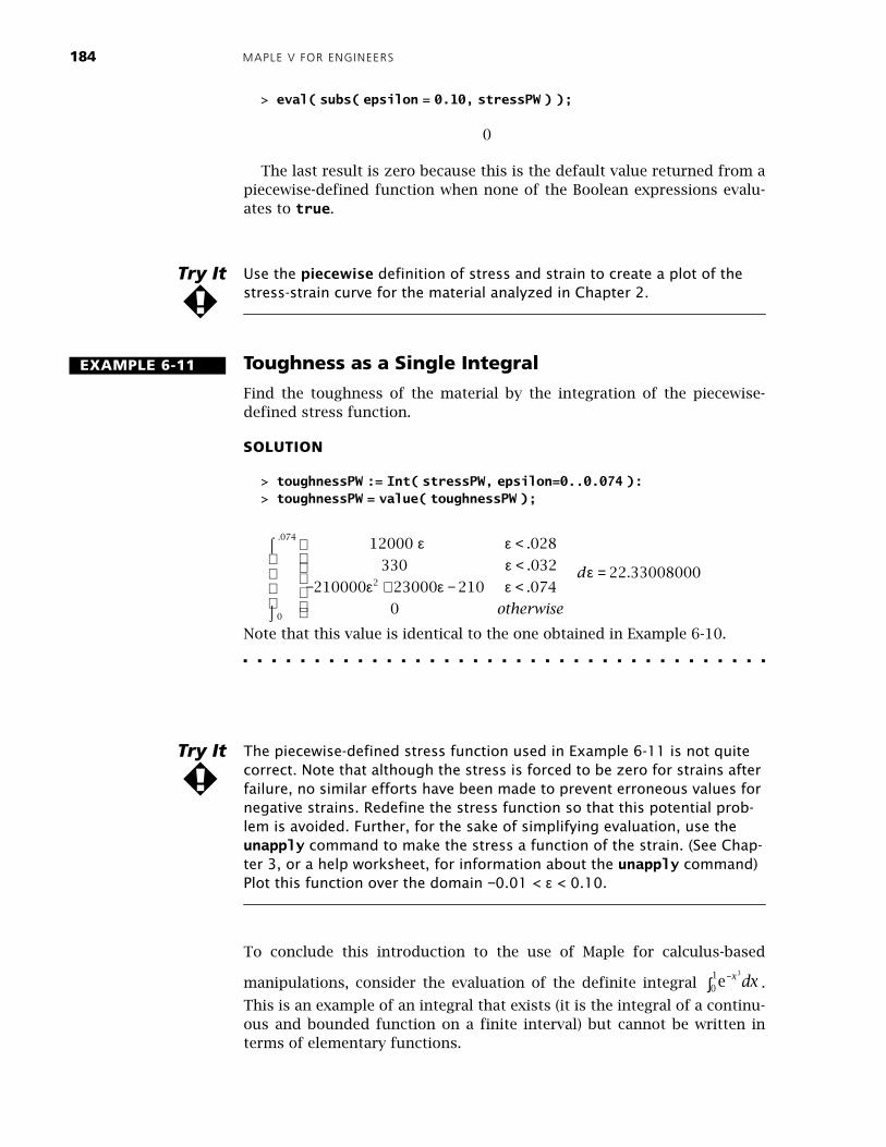
Toughness as a Single Integral

Find the toughness of the material by the integration of the piecewise-defined stress function.

SOLUTION

> toughnessPW := Int( stressPW, epsilon=0..0.074 ):> toughnessPW = value( toughnessPW );

Note that this value is identical to the one obtained in Example 6-10.

The piecewise-defined stress function used in Example 6-11 is not quite correct. Note that although the stress is forced to be zero for strains after failure, no similar efforts have been made to prevent erroneous values for negative strains. Redefine the stress function so that this potential prob-lem is avoided. Further, for the sake of simplifying evaluation, use the unapply command to make the stress a function of the strain. (See Chap-ter 3, or a help worksheet, for information about the unapply command) Plot this function over the domain −0.01 < ε < 0.10.

To conclude this introduction to the use of Maple for calculus-based

manipulations, consider the evaluation of the definite integral .

This is an example of an integral that exists (it is the integral of a continu-ous and bounded function on a finite interval) but cannot be written interms of elementary functions.

Try It

!

EXAMPLE 6-11

12000

330 032 22 33008000210000 23000 210 074

0

2

0

074 ε εε ε

ε ε ε

< < =

− + − <

⌠

⌡

.028

. .

.

.

d

otherwise

Try It

!

e−∫ x dx3

01


The first objective is to understand that the mathematical theory guarantees that the existence of this integral is independent of our ability to express

the value in terms of elementary functions. First, plot y = e−x3 on an

appropriate interval and identify as the area of a plane region.

Then, use the plot to estimate the value of .

Once Maple determines that it is unable to evaluate an expression, theexpression is generally returned unevaluated. A floating-point approxima-tion can be forced with the use of evalf.

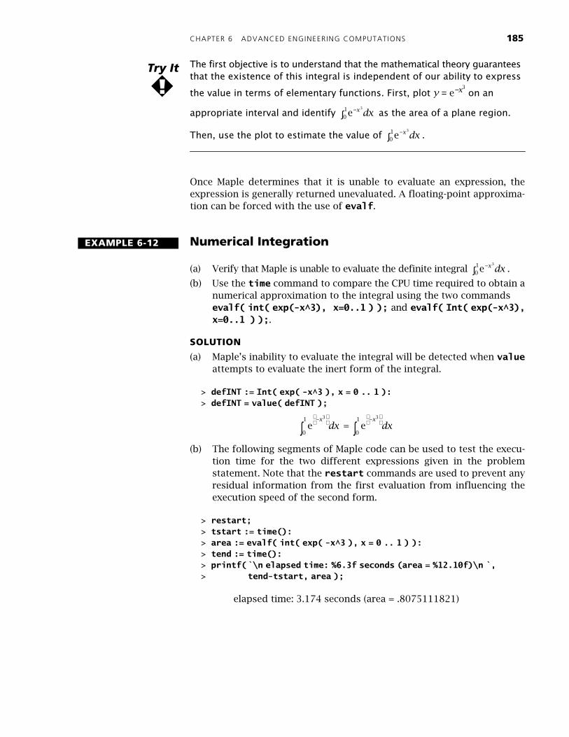
Numerical Integration

(a) Verify that Maple is unable to evaluate the definite integral .

(b) Use the time command to compare the CPU time required to obtain anumerical approximation to the integral using the two commandsevalf( int( exp(-x^3), x=0..1 ) ); and evalf( Int( exp(-x^3),x=0..1 ) );.

SOLUTION

(a) Maple’s inability to evaluate the integral will be detected when valueattempts to evaluate the inert form of the integral.

> defINT := Int( exp( -x^3 ), x = 0 .. 1 ):> defINT = value( defINT );

=

(b) The following segments of Maple code can be used to test the execu-tion time for the two different expressions given in the problemstatement. Note that the restart commands are used to prevent anyresidual information from the first evaluation from influencing theexecution speed of the second form.

> restart;> tstart := time():> area := evalf( int( exp( -x^3 ), x = 0 .. 1 ) ):> tend := time():> printf(`\n elapsed time: %6.3f seconds (area = %12.10f)\n `,> tend-tstart, area );

elapsed time: 3.174 seconds (area = .8075111821)

Try It

!e−∫ x dx

3

01

e−∫ x dx3

01

EXAMPLE 6-12

e−∫ x dx3

01

e−

∫

xdx

3

0

1e

−

∫

xdx

3

0

1


> restart;> tstart := time():> area := evalf( Int( exp( -x^3 ), x = 0 .. 1 ) ):> tend := time():> printf( `\n elapsed time: %6.3f seconds (area = %12.10f)\n `,> tend-tstart, area );

elapsed time: .731 seconds (area = .8075111821)

Note that the values of the integrals are the same up to (at least) 10decimal digits, but that the form that used Int was more than four timesas fast as the evaluation that used int. The difference in execution time isa result of the fact that Maple attempted to evaluate the int commandbefore it realized that a numerical integration was necessary.

The appearance of the output has been improved with the use of the

printf command (see the online help for printf).

You should note that if the integral can be evaluated, then evalf( int( ... ) )returns a floating-point approximation to the evaluated expression; nonumerical integration is performed. To ensure the numerical evaluation ofan integral, evalf( Int( ... ) ) should be used.

6-3 DIFFERENTIAL EQUATIONSThe applications in Chapters 3 and 5 have used differential equations tomodel different aspects of an engineering problem. As these applicationsillustrate, an ability to work with differential equations is essential formany engineers. For these reasons, differential equations are the finalmathematical topic to be discussed in this chapter. Since knowledge ofdifferential equations is not typically a prerequisite for courses thatwould use this module, this introduction will be brief. You are encouragedto revisit this section of the text when you take a course in differentialequations.

A differential equation is an equation that includes the derivative of one ormore unknown functions. The typical objective is to solve the differentialequation—that is, to find the unknown functions that satisfy the differen-tial equation (and any associated initial or boundary conditions). In manycases, it is not possible to find the solution to a differential equation. Inthese instances, the objective may be to use the differential equation toprovide a qualitative description of the solution.

In terms of Maple, the derivatives in a differential equation are enteredusing diff, Diff, or D ; the dsolve command is used to find exact (sym-bolic) and approximate (numeric) solutions to a differential equation; andthe DEtools package, in particular the DEplot command, provides a vari-ety of options for obtaining graphical information about a solution to adifferential equation.

The water quality application in Chapter 5 is based on two differentialequations. The BOD and Streeter–Phelps equations are


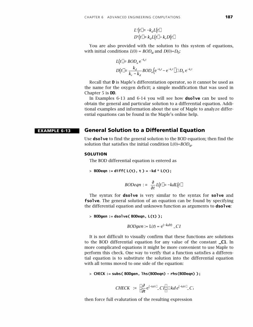
You are also provided with the solution to this system of equations,with initial conditions L(0) = BODu and D(0)=D0:

Recall that D is Maple’s differentiation operator, so it cannot be used asthe name for the oxygen deficit; a simple modification that was used inChapter 5 is DD.

In Examples 6-13 and 6-14 you will see how dsolve can be used toobtain the general and particular solution to a differential equation. Addi-tional examples and information about the use of Maple to analyze differ-ential equations can be found in the Maple’s online help.

General Solution to a Differential Equation

Use dsolve to find the general solution to the BOD equation; then find thesolution that satisfies the initial condition L(0)=BODu.

SOLUTION

The BOD differential equation is entered as

> BODeqn := diff( L(t), t ) = -kd * L(t);

The syntax for dsolve is very similar to the syntax for solve andfsolve. The general solution of an equation can be found by specifyingthe differential equation and unknown function as arguments to dsolve:

> BODgen := dsolve( BODeqn, L(t) );

BODgen := L(t) = e(−kdt) _C1

It is not difficult to visually confirm that these functions are solutionsto the BOD differential equation for any value of the constant _C1. Inmore complicated equations it might be more convenient to use Maple toperform this check. One way to verify that a function satisfies a differen-tial equation is to substitute the solution into the differential equationwith all terms moved to one side of the equation:

> CHECK := subs( BODgen, lhs(BODeqn) - rhs(BODeqn) );

then force full evalutation of the resulting expression

′( ) = − ( )′( ) = ( ) − ( )

L t k L t

D t k L t k D td

d r

L t BOD

D tk

k kBOD D

uk t

d

r du

k t k t k t

d

d r r

( ) =

( ) =−

−( ) +

−

− − −

e

e e e0

EXAMPLE 6-13

BODeqnt

L t kdL t : = ( ) = − ( )∂∂

CHECKt

C1 kd e C1kdt kdt : e _ _=

+−( ) −( )∂∂


> eval( CHECK );

0

Since the result is zero, or an expression that reduces to zero, the equa-tion is satisfied and the function is a solution.

The particular function that also satisfies the initial condition,L(0) = BODu, can be found by substituting the initial condition (and initialtime) into the equation for the general solution, then solving for the con-stant(s). For example, for the BOD problem:

> BODic := L(0) = BODu;

BODic := L(0) = BODu

> BODinit := subs( t=0, BODic, BODgen );

BODinit := BODu = e0 _C1

> solve( BODinit, _C1 );

_C1 = BODu

Thus, the initial condition is satisfied if and only if _C1 = BODu, and theonly function that satisfies the BOD differential equation and the initialcondition is

> BODsoln := subs( ", BODgen );

BODsoln := L(t) = e(−kdt) BODu

A simpler means of obtaining the solution to an initial value problem is tocall dsolve with a first argument that is a set containing both the differ-ential equation and the initial condition.

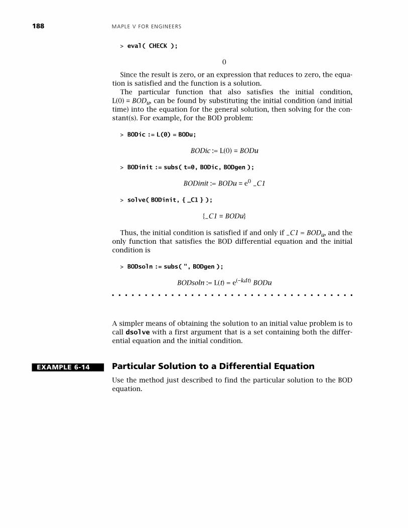
Particular Solution to a Differential Equation

Use the method just described to find the particular solution to the BODequation.

EXAMPLE 6-14


SOLUTION

Using the assignments made in Example 6-13, the set containing the dif-ferential equation and initial condition is

> BODivp := BODeqn, BODic ;

Then, the particular solution can be found with the single command

> dsolve( BODivp, L(t) );

L(t) = e(−kdt) BODu

This solution is, by inspection, the same as the one found in Example 6-13.

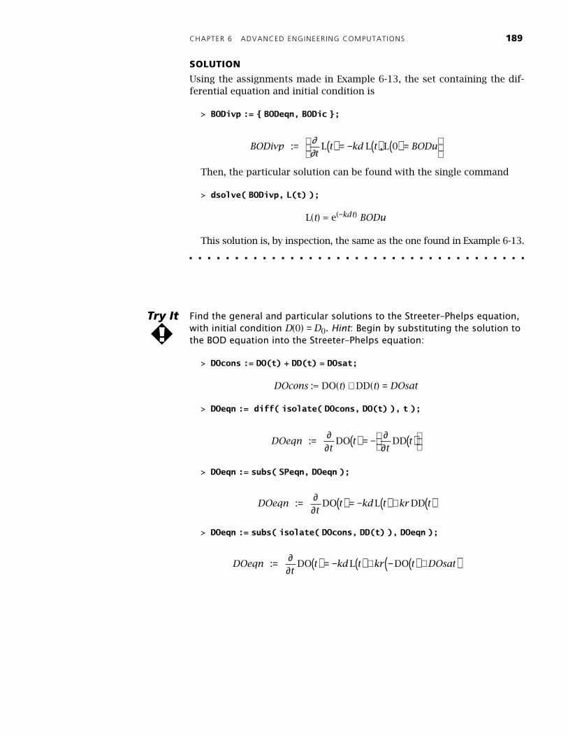
Find the general and particular solutions to the Streeter–Phelps equation, with initial condition D(0) = D0. Hint: Begin by substituting the solution to the BOD equation into the Streeter–Phelps equation:

> DOcons := DO(t) + DD(t) = DOsat;

DOcons := DO(t) + DD(t) = DOsat

> DOeqn := diff( isolate( DOcons, DO(t) ), t );

> DOeqn := subs( SPeqn, DOeqn );

> DOeqn := subs( isolate( DOcons, DD(t) ), DOeqn );

BODivpt

t kd t BODu : L L ,L= ( ) = − ( ) ( ) =

∂∂

0

Try It

!

DOeqnt

tt

t : DO DD= ( ) = − ( )

∂∂

∂∂

DOeqnt

t kd t kr t : DO L DD= ( ) = − ( ) + ( )∂∂

DOeqnt

t kd t kr t DOsat : DO L DO= ( ) = − ( ) + − ( ) +( )∂∂


SUMMARY This chapter demonstrated how Maple can be used in problems thatinvolve complex numbers, calculus, and differential equations. The appli-cation used nodal analysis to investigate a low-pass electrical filter,including the determination of the circuit’s frequency response. Expres-sions for the voltage transfer ratio amplitude and phase were calculatedand plotted. The calculus section focused on problems that involve limits,derivatives, and integrals. Several ways that inert commands can be usedto improve both appearance and efficiency were introduced and demon-strated. Some of the examples revisited applications introduced in earlierchapters. In particular, the toughness of a material was computed bydirect integration after the stress-strain curve was defined as a piecewise-defined function and the biochemical oxygen demand (BOD) and oxygendeficit levels in the water quality application were obtained by solving theBOD and Streeter–Phelps equations.

Keywords

Maple Commands

argumentasymptotic expansioncalculusconjugatedefinite integralderivativedifferential equationdifferentiationgeneral solutionimproper integralindefinite integralinert (unevaluated) form

initial conditioninitial value problemlimitmagnitude (modulus)numerical integration (quadrature)one-sided limitpartial fraction decompositionparticular solution.piecewise-defined functionqualitative analysisseries expansion

@@ (repeated composition operator)abs, conjugate, Re, Imaliasallvalues, RootOfargumentasympt, series, convert,parfraccomplexplot, complexplot3d

(from plots package)DEplot (from the DEtools

package)diff, Diff, Ddsolveevalc,I

int, Intintparts (from the student

package)isolatelimit, Limitmappiecewiseprintfquo, remsemilogplot (from the plots

package)surdtime


References

1. Lopez, R., Maple via Calculus: A Tutorial Approach, New York: Birkhauser, 1994.2. Crawford, R.S. Jr., Waves, New York: McGraw-Hill, 1968, pp. 128–130.3. Johnson, D.E., Hilburn, J.L, Johnson, J.R., and Scott, P.D., Basic Electric Circuit

Analysis, 5th ed. Englewood Cliffs, N.J.: Prentice-Hall, 1995, pp. 284–308, 322–327.

Problems

1. (a) Find the eighth roots of 10. Use nops to verify that the correct number of roots have been found.

(b) Create separate lists containing the real-valued roots and the com-plex-valued roots. Hint: The select and remove commands are recommended for creating subsets of lists or sets as requested in this problem. Further, a common method for testing if an object is complex valued is to use the Boolean function has to check if the object contains I. For example, has( f, I ); returns true if f con-tains I and otherwise returns false.

2. The modulus and argument of a complex number can be used to spec-ify a complex number in polar coordinates. This conversion can be accomplished using Maple’s polar command, whereas conversion from polar to standard form is obtained using evalc. (For additional details, see the help worksheet for polar.)

Let a be a positive number. Find the polar representations of the square, cube, and fourth roots of a. Without using solve, what are the fifth roots of a?

3. Let f be the function introduced in Example 6-6, that is,

.

(a) Use asympt to find the asymptotic expansion of f.

(b) Use series to find the series expansion of f about both x = 0 and x = 3.

(c) Use convert,parfrac to find the partial fraction decomposition of f.

(d) Compare the results found in parts (a), (b), and (c). How hard is it to identify the oblique asymptote in each case? What other infor-mation is contained in these results?

Consult the appropriate help worksheets for information about the syntax and interpretation of results from each of these commands.

4. Note that the function is not defined at x = 0. (See also the

Try It! exercise immediatedly following Example 6-7.)

(a) Plot f and its first three derivatives on the interval [−1, 1].

(b) Is it possible to define f(0) so that f is continuous at x = 0?

(c) Use part (b), and the definition of the derivative, to compute f′(0). Are any derivatives of f continuous at x = 0?

f xx x

x( ) = − +

−2 7 1

3

2

f x x( ) =−

e1

2


5. (a) Compute the definite integral of and

. Cross-check your results using a graph and

interpreting the integral as a (signed) area.

(b) For what values of p does converge?

6. Use the intparts command from the student package to evaluate—

step-by-step—the indefinite integrals (a) and

b) . Does it matter which term in the integrand is chosen

for “u”?

7. The integral was found to be approximately 0.80751118 in

Example 6-12. Another approach to this problem is to expand the inte-grand in a power series (see Problem 3 in this chapter), then integrating the resulting polynomial.

(a) How many terms in the power series expansion of , centered at x = 0, are needed to approximate the value of this integral to five (5) decimal places?

(b) How many terms are needed when the power series is based at x = 1? at x = 1/2?

Hints: The Maple command for computing power series is series (see also Problem 3 in this chapter). Use convert,polynom to convert the result returned by series to a polynomial before integrating.

8. Determine which of the following expressions satisfy the differential

equation :

v1(t) = etsin(2t), v2(t) = e−tsin(t), v3(t) = e−t, v4(t) = cos(t).

9. (a) Another interesting frequency in the analysis of the low-pass filter

is . Find the gain and phase shift for this frequency.

(b) Determine the behavior of both the gain and phase shift as ω increases without bound.

(c) Show that MdB ~ −60log10(ω) + 20(log10(ω′) + 2log10(ω0) ) for

“large” frequencies. (In this context, high-frequency means

>> 1 and >> 1.)

(d) Use the result from part (c) to show that the cut-off frequency, ωc,

satisfies ωc3 = ω′ ω0

2.

(Hint : Use a combination of limit, series, and/or asympt.)

10. a) Produce corrected Bode amplitude plots, and compute the cut-off frequencies when the load resistance is R = 10Ω, R = 1kΩ, R = 500kΩ, R = 1MΩ, R = 10MΩ,and R = 100MΩ. How does changing the load resistance value affect the operation of the low-pass filter?

g xx x

x( ) = − +

−2 7 1

3

2

h xx x

x( ) = − +

−( )2 7 1

3

2

2

2 7 1

3

2

0

3x x

xdxp

− +−( )

⌠

⌡

x x dx2 ln( )∫e cosax bx dx( )∫

e−∫ x dx3

01

e−x3

′′( ) + ′( ) + ( ) =u u ut t t2 2 0

′ =ω RL

ωω0

ωω′


b) The corrected Bode phase plot is a plot of θ (in degrees) vs.

. Create the corrected Bode phase plot for the original

problem and for each of the resistances in part (a).

c) Present the plots in parts (a) and (b) as an animated sequence of plots with increasing values of resistance.

11. Suppose two identical low-pass filters are “cascaded.” Determine the

frequency response function, , for this new composite component.

Does this new component better approximate an “ideal” low-pass filter? (Hint: The output voltage from the first low-pass filter becomes the input voltage to the second low-pass filter.)

12. Note that the solution to the Streeter–Phelps equation is not defined when kd = kr. One possible way to define the solution when kd = kr is

with limits. What function is defined by ? Verify that this

function satisfies the Streeter–Phelps equation when kd = kr.

13. In Chapter 3, Problem 6, you were told that an airplane’s range (s), lift (L), drag (D), thrust-specific fuel consumption (TSFC), take-off mass (m0), and landing mass (m) satisfy the relationship

This relationship is obtained from Breguet’s equation

with initial condition m(0) = m0.

(a) Use Maple to find the particular solution to Breguet’s equation that satisfies the given initial condition.

(b) Note that Breguet’s equation gives the landing mass in terms of the other quantities. Use Maple to rewrite the solution to Breguet’s equation as s = F(m,m0,L,D,V,TSFC,g). Do you obtain the result

stated above (and in Chapter 3)? (Explain any differences.)

(c) The specific form in which the relationship is given depends largely on the way in which it will be used. Give examples of situa-tions in which each of the two forms of the relationship discussed in this problem might be used.

log10 0ω

ω( )

VV

o

i

lim Dkd kr

t→

( )

s

Vmm

L

D gTSFC=

ln0

′( ) = − ( )m

ms

g D s

V L TSFC

advanced engineering computations

Documents