advanced fortran 90/95 programming - university of york · pdf fileguide 47 version 1.0...
TRANSCRIPT
Guide 47 Version 1.0
Advanced Fortran 90/95 Programming
This guide provides an introduction to features of the Fortran 90/95 programming language that are not in its predecessor, Fortran 77. It assumes knowledge at the level of ITS Guide 138, An introduction to programming in Fortran 90, and familiarity with a Fortran 90 or Fortran 95 compiler.
Document code: Guide 47
Title: Advanced Fortran 90/95 Programming
Version: 1.0
Date: 15/05/2008
Produced by: University of Durham Information Technology Service
Copyright © 2008 University of Durham Information Technology Service
Conventions:
In this document, the following conventions are used: A bold typewriter font is used to represent the actual characters you type at the
keyboard.
A slanted typewriter font is used for items such as filenames which you should replace
with particular instances.
A typewriter font is used for what you see on the screen.
A bold font is used to indicate named keys on the keyboard, for example, Esc and
Enter, represent the keys marked Esc and Enter, respectively.
Where two keys are separated by a forward slash (as in Ctrl/B, for example), press
and hold down the first key (Ctrl), tap the second (B), and then release the first key.
A bold font is also used where a technical term or command name is used in the text.
Guide 47: Advanced Fortran 90/95 Programming i
1. Introduction ...................................................................................................................1
2. The KIND Parameter for Intrinsic Data Types .......................................................1
2.1 Selecting precision with the KIND parameter ......................................................1
2.1.1 Making precision portable ...............................................................................1
2.1.2 The KIND number of a variable or constant .................................................2
2.2 Exercises ...................................................................................................................2
3. Derived Data Types and Pointers ............................................................................3
3.1 Derived data types ...................................................................................................3
3.1.1 The component selector ..................................................................................3
3.1.2 Constructors ......................................................................................................4
3.2 Pointers ......................................................................................................................4
3.2.1 The pointer attribute .........................................................................................4
3.2.2 The target attribute ...........................................................................................5 3.2.3 The pointer assignment operator (=>) ...........................................................5
3.2.4 The NULLIFY statement ..................................................................................5
3.2.5 Association status of a pointer........................................................................5
4. Array Features and Operations ................................................................................8
4.1 Arrays of intrinsic type .............................................................................................8
4.2 Array Elements and array subscripts ....................................................................8
4.3 Array Sections ...........................................................................................................8 4.3.1 Subscript triplet .................................................................................................9
4.3.2 Vector subscript ................................................................................................9
4.4 Intrinsic Inquiry Functions for Arrays .....................................................................9
4.5 Array constructors ..................................................................................................10
4.6 Array Initialization and array constants ...............................................................11
4.7 Whole Array Operations ........................................................................................11
4.8 Arrays as subscripts of other arrays ....................................................................12
4.9 Array expressions, elemental array operations and assignment ....................12
4.10 Elemental Intrinsic Functions ................................................................................13
4.11 Mask arrays .............................................................................................................13
4.12 Transformational Intrinsic Functions for numeric arrays ..................................14 4.13 The WHERE construct ..........................................................................................16
4.14 Exercices .................................................................................................................16
5. Dynamic Storage Allocation ....................................................................................17
5.1 About Dynamic memory ........................................................................................17
5.1.1 Dynamic Storage for Arrays ..........................................................................17
5.1.2 The ALLOCATABLE attribute and statement ............................................17
5.1.3 The ALLOCATE statement ...........................................................................17 5.1.4 The allocation status of an array and the ALLOCATED function ............18
5.1.5 De-allocating storage of an array .................................................................18
5.1.6 Variable-sized arrays as component of a structure ...................................18
5.1.7 Dynamic Storage Allocation for Pointers ....................................................18
5.2 Mixing pointers and arrays ....................................................................................19
5.3 Exercises .................................................................................................................19
6. Program Units, Subprograms and Modules ........................................................21
6.1 Fortran Procedures: Functions and Subroutines ...............................................21
6.1.1 The INTENT attribute of procedure arguments .........................................21
Guide 47: Advanced Fortran 90/95 Programming ii
6.2 A comparison of the structure of the three kinds of program units. ............... 22
6.3 Modules ................................................................................................................... 22
6.3.1 Definition of a module.................................................................................... 23
6.3.2 USE of a module ............................................................................................ 23 6.4 Overloading the build-in operators ...................................................................... 24
6.5 Generic Procedures............................................................................................... 25
6.6 Summary ................................................................................................................. 25
6.7 An extended example ........................................................................................... 25
6.8 Exercises ................................................................................................................. 27
Guide 47: Advanced Fortran 90/95 Programming 1
1. Introduction
2. The KIND Parameter for Intrinsic Data Types
Fortran 90/95 introduced a mechanism to specify the precsion of the intrinsic data types with the KIND parameter.
2.1 Selecting precision with the KIND parameter
The terms single and double precision floating point numbers are not precisely defined and depend on the computer. Usually double precision values have approximately twice the precision of single precision values. On many computers single precision floating point numbers are stored in 4 bytes (32 bits) with typically 24 bits for the mantissa and 8 bits for the exponent. This is sufficient for about 7 significant decimal digits and an exponent approximately in the range 10^-38 to 10^38. Double precision has then 64 bits with 53 bits usually devoted to the mantissa and 11 bits to the exponent. This is sufficient to give a precision of approximately 16 significant decimal digits and an exponent in the range 10^-308 to 10^308. However on some computer architectures single and double precision values are represented by 64 and 128 bits respectively. Therefore a program that runs properly in single precision on such a computer may need double precision when run on a 32 bit computer.
To make Fortran programs more portable between different computer systems the KIND parameter for intrinsic data types was introduced. Single and double precision real numbers are different kinds of the real data type, specified with a different KIND number. On some systems it indicates the number of bytes of storage for the type, however the standard does not require this. Therefore the KIND number itself is not portable between computer architectures but is used to distinguish between different kind of literal constants by appending it to the value separated by an underscore. For example
INTEGER, PARAMETER :: single = 4
REAL ( KIND = single ) :: a , b
a = 1.2_single , b = 34.56E7_4
If the KIND number for a variable or constant is not specified then it is of the default kind and its value depends on the computer platform.
2.1.1 Making precision portable
Since the KIND number is not portable, Fortran provides functions to specify the required precision across platforms. The compiler will then select the smallest value of the KIND parameter that still can represent the requested precision, or otherwise it will fail to compile. In the case of integers the number of digits can be specified with the SELECED_INT_KIND function which has as argument the number of digits (ignoring the sign) and returns a default integer with the minimum KIND number.
Example
To specify an integer type with up to 9 decimal digits the following declarations can be used:
INTEGER, PARAMETER :: long = SELECED_INT_KIND ( 9 ) INTEGER ( KIND = long ) :: n , m
n = 1_long , m = -10_long.
Guide 47: Advanced Fortran 90/95 Programming 2
The range of values for n and m is thus between -999999999 and +999999999.
The corresponding intrinsic function for real numbers is
SELECTED_REAL_KIND ( p , r )
which returns the minimum KIND number necessary to store real numbers with a precision of p decimal digits and an exponent in the range 10^-r to 10^r.
Example INTEGER, PARAMETER :: dble = SELECTED_REAL_KIND ( 15, 300 ) REAL ( KIND = dble ) :: planck_constant = 6.631 * 10 ** -31_dble PRINT *, 'Planck's constant is ', planck_constant
2.1.2 The KIND number of a variable or constant
Fortran 90/95 also provides an intrinsic function to determine the kind number of any variable or constant.
WRITE ( *, „( „‟The KIND number for default integer is „‟ , I2) „ ) KIND ( 0 )
WRITE ( *, „( „‟The KIND number for default single precision is‟„ , I2) „ ) KIND ( 0.0 )
WRITE ( *, „( „‟The KIND number for default double precision is „„ , I2) „ ) KIND ( 0.0D0 )
On most systems this will return the values 4, 4 and 8 respectively which could, but not have to be, the number of bytes used for storage.
2.2 Exercises
1. Write a program that prints the KIND value for default integers, real and double precision numbers on your computer.
2. Write a program to find the largest possible value of the KIND number for integers that your computer allows.
Guide 47: Advanced Fortran 90/95 Programming 3
3. Derived Data Types and Pointers
3.1 Derived data types
It is possible to create new data types in Fortran 90/95, alongside the intrinsic data types. These are called derived data types and are build from any number of components. The components can be intrinsic data types and any other derived data types. This is an example of an object oriented feature, sometimes called abstract data types.
TYPE [ :: ] type-name component-definitions END TYPE [ type-name ]
Example
TYPE :: Person
CHARACTER ( LEN = 10 ) :: name
REAL :: age
INTEGER :: id
END TYPE Person
Declaration of a variable (or object) of the type type-name is as follows TYPE ( type-name ) :: var1, var2, ... Example
TYPE ( Person ) :: john , mary
Each instance of a derived data type is called a structure. Arrays of derived data types can be defined as well, TYPE ( type-name ) , DIMENSION ( dimensions ) :: array-name Example
TYPE ( Person ), DIMENSION ( 10 ) :: people
3.1.1 The component selector
The components of a structure can be accessed with the component selector. This consists of the name of the variable (structure) followed by a percentage sign and the component name var % component
and in the case of an array of a derived type
array-name ( subscripts ) % component
Example
PRINT*, „John‟‟s age is „, john%age
PRINT*, „The name of person number 2 is „, people(2)%name
Guide 47: Advanced Fortran 90/95 Programming 4
3.1.2 Constructors
These can be used to initialise a structure, that is, its components.
When struct-name is of derived type type then
struct-name = type ( component-1 , ... , component-n )
Note
All components of type must be present with a value in the argument list.
The order of the arguments has to be the same as the order in which the components are defined in the derived type definition.
Example
john = Person ( „Jones‟, 21, 7 ) ; mary = Person ( „Famous‟, 18, 9 )
people ( 5 ) = Person ( „Bloggs‟, 45, 3045 )
people ( 6 ) = john
3.2 Pointers
3.2.1 The pointer attribute
Pointers are special kinds of variables (objects) that can be made to refer to other variables (of the same type) or other pointers (of the same type). Storage for pointers is defined by assignment to a target or with the ALLOCATE statement (Sect ).
assignin
p => t where t is a target attribute makes p an alias of t
provide information where an object can be found. They are used to allocate unnamed storage and to pass arrays by reference in subprograms.
Pointers can be considered as variables that have certain variables as values. This requires the declaration of the pointer and the target attribute. The type of the objects that can a pointer can point at has to be stated in its declaration. Pointer objects are declared with the POINTER attribute type , POINTER :: ptr [, ptr ] type , DIMENSION ( : [, ; ] ) , POINTER :: ptr [, ptr ] where ptr is a pointer to scalars and arrays respectively.
Alternatively, a POINTER statement can be used, after the object has been declared:
type :: ptr [, ptr ] POINTER :: ptr [, ptr ] Note:
type can be a structure (derived type).
If the pointer is an array then only the rank has to be declared and the bounds are taken from the array that it points at.
Guide 47: Advanced Fortran 90/95 Programming 5
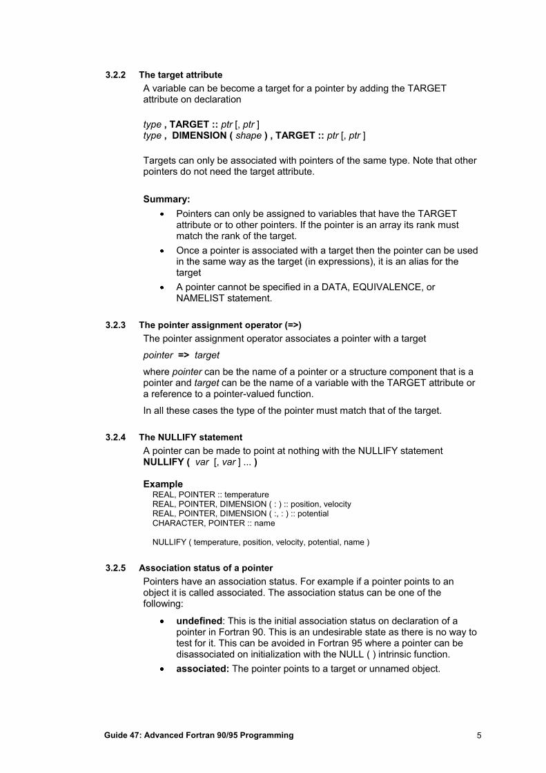
3.2.2 The target attribute
A variable can be become a target for a pointer by adding the TARGET attribute on declaration
type , TARGET :: ptr [, ptr ] type , DIMENSION ( shape ) , TARGET :: ptr [, ptr ]
Targets can only be associated with pointers of the same type. Note that other pointers do not need the target attribute.
Summary:
Pointers can only be assigned to variables that have the TARGET attribute or to other pointers. If the pointer is an array its rank must match the rank of the target.
Once a pointer is associated with a target then the pointer can be used in the same way as the target (in expressions), it is an alias for the target
A pointer cannot be specified in a DATA, EQUIVALENCE, or NAMELIST statement.
3.2.3 The pointer assignment operator (=>)
The pointer assignment operator associates a pointer with a target
pointer => target
where pointer can be the name of a pointer or a structure component that is a pointer and target can be the name of a variable with the TARGET attribute or a reference to a pointer-valued function.
In all these cases the type of the pointer must match that of the target.
3.2.4 The NULLIFY statement
A pointer can be made to point at nothing with the NULLIFY statement NULLIFY ( var [, var ] ... ) Example REAL, POINTER :: temperature REAL, POINTER, DIMENSION ( : ) :: position, velocity REAL, POINTER, DIMENSION ( :, : ) :: potential CHARACTER, POINTER :: name NULLIFY ( temperature, position, velocity, potential, name )
3.2.5 Association status of a pointer
Pointers have an association status. For example if a pointer points to an object it is called associated. The association status can be one of the following:
undefined: This is the initial association status on declaration of a pointer in Fortran 90. This is an undesirable state as there is no way to test for it. This can be avoided in Fortran 95 where a pointer can be disassociated on initialization with the NULL ( ) intrinsic function.
associated: The pointer points to a target or unnamed object.
Guide 47: Advanced Fortran 90/95 Programming 6
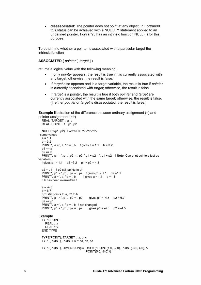
disassociated: The pointer does not point at any object. In Fortran90 this status can be achieved with a NULLIFY statement applied to an undefined pointer. Fortran95 has an intrinsic function NULL ( ) for this purpose.
To determine whether a pointer is associated with a particular target the intrinsic function ASSOCIATED ( pointer [, target ] ) returns a logical value with the following meaning:
If only pointer appears, the result is true if it is currently associated with any target; otherwise, the result is false.
If target also appears and is a target variable, the result is true if pointer is currently associated with target; otherwise, the result is false.
If target is a pointer, the result is true if both pointer and target are currently associated with the same target; otherwise, the result is false. (If either pointer or target is disassociated, the result is false.)
Example Illustration of the difference between ordinary assignment (=) and pointer assignment (=>) REAL, TARGET :: a, b REAL, POINTER :: p1, p2 NULLIFY(p1, p2) ! Fortran 90 ????????? ! some values a = 1.1 b = 3.2 PRINT*, 'a = ', a, ' b = ', b ! gives a = 1.1 b = 3.2 p1 => a p2 => b PRINT*, 'p1 = ', p1, ' p2 = ', p2, ' p1 + p2 = ', p1 + p2 ! Note: Can print pointers just as
variables! ! gives p1 = 1.1 p2 =3.2 p1 + p2 = 4.3 p2 = p1 ! p2 still points to b! PRINT*, 'p1 = ', p1, ' p2 = ', p2 ! gives p1 = 1.1 p2 =1.1 PRINT*, 'a = ', a, ' b = ', b ! gives a = 1.1 b =1.1 ! b has been overwritten ! a = -4.5 b = 6.7 ! p1 still points to a, p2 to b PRINT*, 'p1 = ', p1, ' p2 = ', p2 ! gives p1 = -4.5 p2 = 6.7 p2 => p1 PRINT*, 'a = ', a, ' b = ', b ! not changed PRINT*, 'p1 = ', p1, ' p2 = ', p2 ! gives p1 = -4.5 p2 = -4.5
Example TYPE POINT REAL :: x REAL :: y END TYPE TYPE(POINT), TARGET :: a, b, c TYPE(POINT), POINTER :: pa, pb, pc TYPE(POINT), DIMENSION(3) :: tri1 = (/ POINT(1.0, -2.0), POINT(-3.0, 4.0), & POINT(5.0, -6.0) /)
Guide 47: Advanced Fortran 90/95 Programming 7
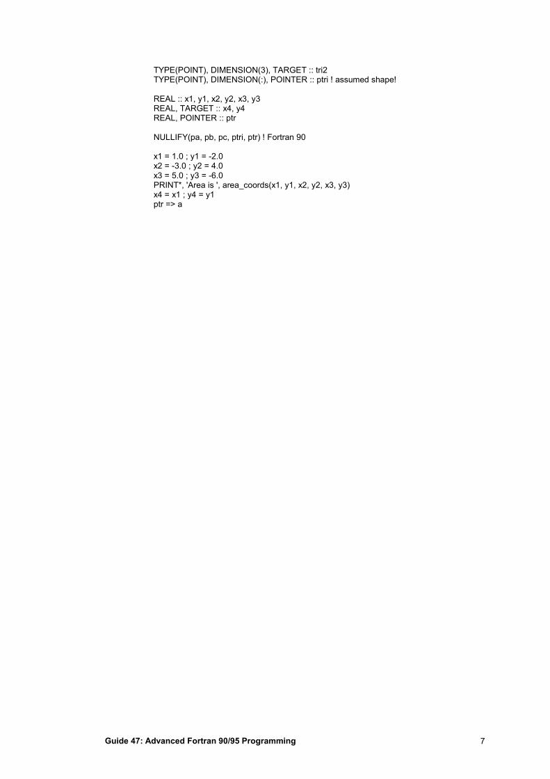
TYPE(POINT), DIMENSION(3), TARGET :: tri2 TYPE(POINT), DIMENSION(:), POINTER :: ptri ! assumed shape! REAL :: x1, y1, x2, y2, x3, y3 REAL, TARGET :: x4, y4 REAL, POINTER :: ptr NULLIFY(pa, pb, pc, ptri, ptr) ! Fortran 90 x1 = 1.0 ; y1 = -2.0 x2 = -3.0 ; y2 = 4.0 x3 = 5.0 ; y3 = -6.0 PRINT*, 'Area is ', area_coords(x1, y1, x2, y2, x3, y3) x4 = x1 ; y4 = y1 ptr => a
Guide 47: Advanced Fortran 90/95 Programming 8
4. Array Features and Operations
4.1 Arrays of intrinsic type
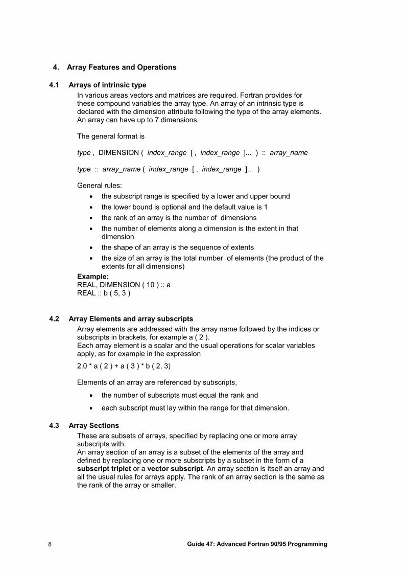
In various areas vectors and matrices are required. Fortran provides for these compound variables the array type. An array of an intrinsic type is declared with the dimension attribute following the type of the array elements. An array can have up to 7 dimensions. The general format is type , DIMENSION ( index_range [ , index_range ]... ) :: array_name type :: array_name ( index_range [ , index_range ]... ) General rules:
the subscript range is specified by a lower and upper bound
the lower bound is optional and the default value is 1
the rank of an array is the number of dimensions
the number of elements along a dimension is the extent in that dimension
the shape of an array is the sequence of extents
the size of an array is the total number of elements (the product of the extents for all dimensions)
Example: REAL, DIMENSION ( 10 ) :: a REAL :: b ( 5, 3 )
4.2 Array Elements and array subscripts
Array elements are addressed with the array name followed by the indices or subscripts in brackets, for example a ( 2 ). Each array element is a scalar and the usual operations for scalar variables apply, as for example in the expression
2.0 * a ( 2 ) + a ( 3 ) * b ( 2, 3) Elements of an array are referenced by subscripts,
the number of subscripts must equal the rank and
each subscript must lay within the range for that dimension.
4.3 Array Sections
These are subsets of arrays, specified by replacing one or more array subscripts with. An array section of an array is a subset of the elements of the array and defined by replacing one or more subscripts by a subset in the form of a subscript triplet or a vector subscript. An array section is itself an array and all the usual rules for arrays apply. The rank of an array section is the same as the rank of the array or smaller.
Guide 47: Advanced Fortran 90/95 Programming 9
4.3.1 Subscript triplet
These have the form
subscript-1 : subscript-2 : stride
This works much like an implied DO loop.
Example REAL :: a ( 3, 5 ), b ( 2, 2 ) , c ( 5 ) The array a has the structure a(1,1) a(1,2) a(1,3) a(1,4) a(1,5) a(2,1) a(2,2) a(2,3) a(2,4) a(2,5) a(3,1) a(3,2) a(3,3) a(3,4) a(3,5) Then the array section a ( 1 : 2, 2 : 4 : 2 ) can be assigned to array b which is conformable b = a ( 1 : 2, 2 : 4 : 2 ) The array b has the elements a(1,2) a(1,4) a(2,2) a(2,4)
An array section with rank one is
c = a ( 2 , : ) Example INTEGER :: i REAL :: a ( 10) = (/ ( REAL( i ) , i = 1, 10 ) /) PRINT*, a a ( 2 : 10 : 2 ) = a ( 1 : 9 : 2 ) PRINT*, a
4.3.2 Vector subscript
A vector subscript is a rank one integer array where the elements are the subscripts that specify the array section. For example to access the elements a(1, 2) , a(2, 2) , a(1, 4) and a( 2, 4) you can use
INTEGER :: p = (/ 2 , 4 /) and set
B = a ( (/ 1 , 2 /) , p )
4.4 Intrinsic Inquiry Functions for Arrays
There are number of intrinsic functions that can be used to inquire about the general properties of a given array, namely its rank, extents etc. SIZE ( array-name [ , dim ] )
This function returns a default integer which is the number of elements (the size) of the array if the dimension number dim is absent, or, the extent of the array along dimension dim if it is present.
Returns a default INTEGER
dim is an optional integer, if it is absent its values is assumed to be one
If dim is present it must be a valid dimension of array.
Information about the shape of an array can be found with some intrinsic functions.
Example SIZE ( a ) returns 10, SIZE ( b ) returns 15 whereas SIZE ( b, 2 ) returns 3.
Guide 47: Advanced Fortran 90/95 Programming 10
SHAPE ( array-name )
returns a one dimensional array of default integers with extent ( = size) equal to the rank of array-name and the elements give the extent of array-name in each dimension Example REAL :: s1( 1 ) , s2( 2 ) s1 ( 1 ) = SHAPE ( a ) ! gives the array s1 with one element and value s1( 1 ) equal to 10. s_2 = SHAPE( b ) returns the rank-one array s2 with elements 5 and 3. LBOUND ( array-name [ , dim ] ) when the dimension dim is absent returns a rank-one default integer array holding the lower bound for the dimensions when dim is present returns a default integer with as value the lower bound for the dimension UBOUND ( array--name [ , dim ]) as for LBOUND except it returns upper bounds.
UBOUND ( array-name , dimension ) type , DIMNSION ( range ) :: array INTEGER, OPTIONAL :: dim
RESHAPE ( array , shape , pad , order )
Elements of an array are specified by subscripts the number of subscripts must equal the rank each subscript must lay within the range for that dimension
4.5 Array constructors
Array constructors can be used to initialize or assign values to a whole array or array section. The values are given as a list between the delimiter pair (/ and /) as
(/ value-list /)
where value in value-list is either an expression or an implied DO loop. The values in the list are used in array element order and define a rank one array. The implied DO loops may be nested.
Example REAL :: a ( 5 ) , b ( 3 )
a = (/ 1.0, 2.0, 3.0, 4.0, 5.0 /)
PRINT*, a
b = (/ ( REAL( i ), i = 1, 3 ) /)
PRINT*, b
An array of rank greater than one can be constructed with the intrinsic function RESHAPE.
Example REAL :: a ( 3, 5 )
INTEGER :: i, j a = RESHAPE ( (/ ( REAL( i ), i = 1, 15 ) /) , (/ 3, 5 /) )
PRINT*, ( ( a( i , j ) , j = 1, SIZE( a, 2) ), i = 1, SIZE( a , 1 )
Guide 47: Advanced Fortran 90/95 Programming 11
The first argument of the RESHAPE function is the array that has to be reshaped; the second argument specifies that the set of 15 real numbers are stored as an array with 3 rows and 5 columns.
Array constructors can also be used with constant objects of derived type in the value list.
4.6 Array Initialization and array constants
Just as with scalar variables it is possible to initialize arrays during declaration and to define constant arrays. This can be done with an array constructor or with a whole array assignment. Fortran 77 has the DATA statement for initialization of
arrays
Example INTEGER, PARAMETER :: three = 3
INTEGER :: I , j REAL :: b ( three ) = (/ ( REAL( i ), i = 1, three ) /) REAL, PARAMETER :: a ( 5 ) = (/ 1.0, 2.0, 3.0, 4.0, 5.0 /)
REAL, PARAMETER :: c( 5, 6 ) = 1.0 ! all elements initialized to 1.0
REAL :: d ( -3 : 3 , 10 )
DATA ( (d ( i , j ) , I = -3 , 3 ), j = 1, 10 ) / 70 * 1.0 /
4.7 Whole Array Operations
In order to simplify code arithmetic operations on arrays can be written symbolically in the same fashion as mathematical expressions. This also reduces the risk of coding errors but a more important reason is that the compiler can optimize the order in which the underlying scalar operations on the array elements are executed on the target computer architecture. Array expressions and assignment An array expression may be assigned to an array of the same shape. Such an assignment is done on an element by element basis. To be able to operate on an array element by element the two arrays must have the same shape. Two arrays are called conformable if they have the same shape. A scalar is conformable with any array.
Note: The correspondence is by position in the extent of each dimension, not by subscript value. For example, the two arrays declared as
REAL, DIMENSION :: a( -2 : 2 , 3 ), b( 5 , 3 )
are conformable. Example: A system of N point particles in 3D space is described by position and velocity vectors and interact through a mutual potential field. The data declarations to describe this are INTEGER :: N = 100 ! Initialised here to some value. REAL, DIMENSION :: r ( 3, N ), v ( 3, N ), F ( 3, N, N ) INTEGER :: i, j ! some operations: ! add postion of particle 1 and 2: SUM = R(:, 1) + R(:, 2)
Guide 47: Advanced Fortran 90/95 Programming 12
The distance between particles i and j is
d (:) = r (:, i) - r (:, j) d = SQRT ( ( r (:, i) - r (:, j) ) ** 2 )
Often the velocity of a particle is approximated by a finite difference. If r_old ( : , i ) and r_new ( : , i ) are the position vectors of particle i at times t1 and t2 respectively then its average velocity vector may be approximated by the expression v_average ( : , i ) = ( r_new ( : , i ) - r_old ( : , i ) ) / ( t2 - t1 )
In fact this can be written as a whole array operations for all particles: v_average ( : , : ) = ( r_new ( : , : ) - r_old ( : , : ) ) / ( t2 - t1 )
However whole array multiplication is not what might be expected.
Example The Inner product of two vectors. REAL :: x ( 3 ), y (3 ), prod( 3 ) REAL :: sum prod = x * y
sum = SUM ( x * y )
The product of the arrays x and y is evaluated on an element by element basis and assigned to prod with elements prod ( i ) = x (i ) * y ( i ). The intrinsic SUM function returns the sum of the elements of prod.
4.8 Arrays as subscripts of other arrays
The range of an array can also be defined with a rank-one integer array INTEGER, DIMENSION :: odd ( 5 ) = (/ ( i, i= 1, 9, 2 ) /), even ( 5 ) = (/ ( i, i= 2, 10, 2 ) /) ! same as odd = (/ 1, 3, 5, 7, 9 /) ; even = (/ 2, 4, 6, 8, 10 /) REAL :: a ( 10 ) a ( odd ) = 1.0 a ( even ) = - 1.0 PRINT*, a
The range of an array can also be defined with a rank-one integer array
INTEGER, DIMENSION :: odd ( 5 ) = (/ ( i, i= 1, 9, 2 ) /), even ( 5 ) = (/ ( i, i= 2, 10, 2 ) /) ! same as odd = (/ 1, 3, 5, 7, 9 /) ; even = (/ 2, 4, 6, 8, 10 /) REAL, DIMENSION :: a ( 10 ), b ( 10, 10 ) a ( odd ) = 1.0 a ( even ) = - 1.0 ! this creates a 'checker board' pattern of one and zeros b ( odd, even ) = 1.0 b ( even, odd ) = 0.0 ! also a = b ( 1, even ) b ( even, odd ) = 1.0 - b ( odd, even)
4.9 Array expressions, elemental array operations and assignment
Arithmetic operations on arrays can be written symbolically in the same fashion as mathematically. This also reduces the risk of coding errors but more importantly reason is that the compiler can optimize the order in which the scalar operations are executed as it sees fit for the target computer architecture. This includes addition, subtraction, multiplication, division and exponentiation
Guide 47: Advanced Fortran 90/95 Programming 13
An array expression may be assigned to an array of the same shape. Such an assignment is done on an element by element basis.
The scalar arithmetic operations of addition, subtraction, multiplication, division and exponentiation can be generalized to arrays. These are called elemental operations because they work on an element by element basis. For example REAL :: a ( 3, 5), b ( 3, 5 )
a + b
The sum is an array expression with elements a ( i, j ) + b ( i, j ) with 1 <= i <= 3 and 1 <= j <= 5. To be able to operate on two arrays on an element by element basis they both must have the same shape. Two arrays are called conformable if they have the same shape. A scalar is conformable with any array. Note: The correspondence is by position in the extent in each dimension, not by subscript value. For example the two arrays a ( 5, 6 ) and b ( -2 : 2 , 0 : 5) have the same shape although their lower and upper bound values differ. Note: Whole array multiplication and division are not what might be expected. For example the multiplication of two square matrices a and b ( rank 2 arrays with same extent in each dimension ) would not form a product with the usual rule of matrix multiplication. Instead the result would be a square matrix with elements a ( i, j ) * b ( i, j ).
4.10 Elemental Intrinsic Functions
Most intrinsic functions for scalars can also be applied to arrays. The intrinsic function will be applied on an element by element basis. Usually the same result could be obtained by applying the intrinsic functions inside a series of nested DO loops. Example: b = SIN ( a ) c = ABS ( a + SQRT ( b ) ) This requires a , b and c all having the same shape.
elemental, each element is operated on in the same way
singel operation to the whole array, e.g. the sum of all elements
operations on indvidual elements
match certain conditions
4.11 Mask arrays
These are arrays of LOGICAL type and are used to select a subset of array elements for which the correponding mask array element is true. This is usefull in whole array operations when an operation should only be applied array elements that satisfy some condition. For example INTEGER :: i REAL :: a ( 5 ) = (/ ( (-1.0 ) ** i , i = 0, 4 ) /) LOGICAL :: lg ( SIZE ( a ) ) PRINT*, a lg = a > 0.0 PRINT*, lg
Guide 47: Advanced Fortran 90/95 Programming 14
4.12 Transformational Intrinsic Functions for numeric arrays
The following intrinsic functions have an array of numeric type as argument and some optional arguments to control the behaviour of the function.
They all return a scalar result of the same type as the array.
If the dimension dim is present then the function will be applied only to the elements in that dimension.
If the LOGICAL array mask is present then it must be conformable to array and the function will be applied only to those elements for which the corresponding element of the mask array is true.
SUM ( array [ , DIM = dim ] ) returns the sum of the elements of a numeric type array and zero if its size is zero PRODUCT ( array [ , DIM = dim ] ) returns the sum of the elements of a numeric type array and zero if its size is zero MAXVAL ( array [ , DIM = dim ] ) returns the maximum value MINVAL ( array [ , DIM = dim ] [ , MASK = mask ] ) returns the minimum value MAXLOC ( array [ , MASK = mask ] ) returns a rank-one with the rank of array as size and the subscripts of the maximum value as elements MINLOC( array [ , MASK = mask ] ) as MAXLOC except for the minimum value DOT_PRODUCT gives the sum of all products of corresponding elements as in a ( i, j ) * b ( i, j ) with 1 <= i <= 10, 1 <= j < = 20 Example REAL, DIMENSION ( 5 ) :: a = (/ 1.2, -0.3, 0.0, 1E-5, 1.6E3 /) REAL :: min INTEGER :: loc ( SIZE ( SHAPE ( a ) ) ) ! find the smallest positive number in this array and its index PRINT*, a > 0.0 min = MINVAL ( a, a > 0.0 ) loc = MINLOC ( a , a > 0.0 ) PRINT*, min, loc, a ( loc ( 1 ) )
single argument case have an array as argument and some optional arguments to control the behaviour of the function return a scalr result ALL ( mask [ , dim ] ) ANY ( mask [ , dim ] )
in the following mask is of type logical, it can also be an expression ALL(mask, dim) ANY(mask, dim)
Guide 47: Advanced Fortran 90/95 Programming 15
Returns a logical array
Example: If A(1:10, -4:4) is a REAL array then ANY(A(:,:) < 0.0) will return .TRUE. if any array elements are negative, otherwise .FALSE. If a set of 10 files have to be opened and the STATUS value returned for each file is stored in a vector IOSVECTOR(10) then ANY(IOSVECTOR(:) /= 0) will return .TRUE. if there was an error for at least one file.
COUNT ( mask [ , DIM = dim ] ) default integer the number of elements of mask that are .TRUE. mask a LOGICAL array SUM ( array [ , DIM = dim ] ) returns the sum of the elements of a numeric type array and zero if its size is zero PRODUCT ( array [ , DIM = dim ] ) returns the sum of the elements of a numeric type array and zero if its size is zero MAXVAL ( array [ , DIM = dim ] ) returns MINVAL ( array [ , DIM = dim ] [ , MASK = mask ] ) returns
CEILING(array) integer elemental fnx array of type real, returns scalar of type integer, which is the least integer greater than or equal to array FLOOR(array) returns the greatest default??? integer less than or equal to array
Arithmetic operations on elements of a single matrix
SUM(array, dim, mask) type[, DIMENSION(:[,:])] :: array INTEGER, OPTIONAL :: dim PRODUCT(
Operations on multiple arrays
MERGE(truearray,falsearray,maskarray) All arguments must have the same shape, the return type is of that shape. maskArray is logical
MERGE(true, false, mask) elemental function true and false are of same type and shape return type is same type and shape as parameters true and false mask is type logical and same shape as true and false Example: INTEGER, DIMENSION :: A(10) = / 0,1, 2, 3,4, 5, 6,7 ,8 ,9/ A(:) = MERGE(0, A(:), A(:) > 5) ! sets all array values greater than 5 to zero: matrix transpose
Guide 47: Advanced Fortran 90/95 Programming 16
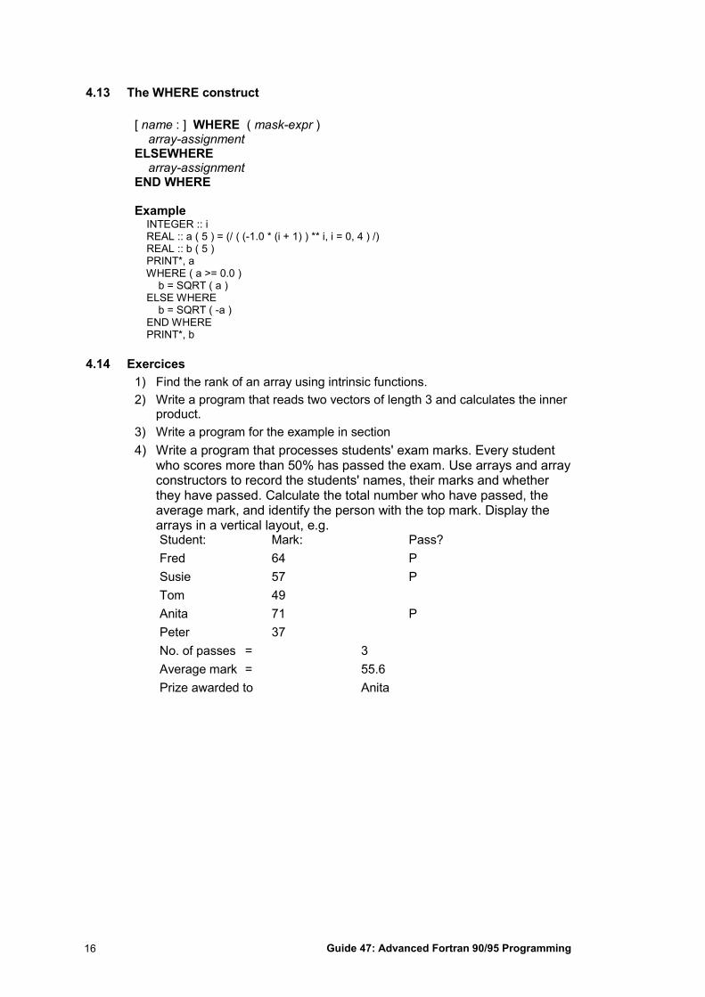
4.13 The WHERE construct
[ name : ] WHERE ( mask-expr ) array-assignment ELSEWHERE array-assignment END WHERE Example INTEGER :: i REAL :: a ( 5 ) = (/ ( (-1.0 * (i + 1) ) ** i, i = 0, 4 ) /) REAL :: b ( 5 ) PRINT*, a WHERE ( a >= 0.0 ) b = SQRT ( a ) ELSE WHERE b = SQRT ( -a ) END WHERE PRINT*, b
4.14 Exercices
1) Find the rank of an array using intrinsic functions.
2) Write a program that reads two vectors of length 3 and calculates the inner product.
3) Write a program for the example in section
4) Write a program that processes students' exam marks. Every student who scores more than 50% has passed the exam. Use arrays and array constructors to record the students' names, their marks and whether they have passed. Calculate the total number who have passed, the average mark, and identify the person with the top mark. Display the arrays in a vertical layout, e.g. Student: Mark: Pass?
Fred 64 P
Susie 57 P
Tom 49
Anita 71 P
Peter 37
No. of passes = 3
Average mark = 55.6
Prize awarded to Anita
Guide 47: Advanced Fortran 90/95 Programming 17
5. Dynamic Storage Allocation
5.1 About Dynamic memory
The rules for allocating storage are very similar for array variables and pointer variables. The main differences are in the fact that pointers are associated with unnamed storage (that is storage not assigned to an allocatable variable) and the allocation status intermixes with the association status.
Also, all pointers are implicitly ALLOCATABLE whereas variables need that attribute.
5.1.1 Dynamic Storage for Arrays
Often the size of an array is only known after data has been read or as the result of some calculation.
Allocatable arrays are arrays whose rank is declared but the extent (bounds) in each dimension is determined at runtime (dynamically). An array that is not a dummy argument of a procedure or the return value of an array valued function. (later)
5.1.2 The ALLOCATABLE attribute and statement
Use of the ALLOCATABLE attribute in the declaration of an array specifies the array as allocatable. The formal notation is: type , DIMENSION( shape ), ALLOCATABLE, [ SAVE ] :: array_name , [ array_name ] ... type , ALLOCATABLE, [ SAVE ] :: array_name ( shape ) , [ array_name ( shape ) ] ... This is an example of a deferred-shape array as the actual shape will be defined until storage is allocated. The initial allocation status of such an array is “not currently allocated”. Allocatable arrays are useful to save large arrays between procedure calls.
5.1.3 The ALLOCATE statement
This is defined with the ALLOCATE statement and keyword ALLOCATE ( array-name ( shape ) [ array_name ( shape )] ... [ , STAT = status ] ) array-name is the name of an array, but which cannot be a structure component.
INTEGER status
must not be allocated in the same ALLOCATE statement as where it is used.
If the STAT = statement is absent and the ALLOCATE produces an error then the program will terminate with an error.
The STAT return values are: 0 indicates success. > 0 indicates a system dependent runtime error.
Guide 47: Advanced Fortran 90/95 Programming 18
Example REAL, ALLOCATABLE :: a(:), b(:) INTEGER :: err ALLOCATE(a(1:10), b(1:10), STAT=err)
! should test for err /= 0 here
If more than one array, dimensions cannot depend on each other: ALLOCATE(a(1:10), b(SIZE(a)), STAT=err)
Note: It is not allowed to allocate an array that is already in the allocated state and this will generate a run time error. (See )
5.1.4 The allocation status of an array and the ALLOCATED function
It is always possible to use the intrinsic logical function ALLOCATED to check the allocation status of an array. ALLOCATED ( array_name ) This function will return true if the array is allocated, otherwise false.
5.1.5 De-allocating storage of an array
Once an allocatable array is no longer required the allocated memory should be released to the heap. This is to ensure that no unused memory will be held by the program. This is called de-allocating the array and the DEALLOCATE statement is the counterpart of the ALLOCATE statement. Once the array has been deallocated any data in it is no longer accessible
DEALLOCATE ( array_name ( shape ) [ array_name ( shape )] ... [ , STAT = status ] ) Again the STAT = clause is optional.
5.1.6 Variable-sized arrays as component of a structure
It is not allowed to declare an array allocatable if it is a component of a structure. In this case an array pointer must be used, see Section .
5.1.7 Dynamic Storage Allocation for Pointers
As was explained in the beginning of this chapter, pointers are by default allocatable and this applies to any type of pointer. A number of examples are given below. This reflects the various structures of the storage allocated.
REAL, POINTER :: temperature REAL, POINTER, DIMENSION ( : ) :: position, velocity REAL, POINTER, DIMENSION ( : , : ) :: potential CHARACTER, POINTER :: name Example NULLIFY ( temperature, position, velocity, potential, name )
An object pointer can be allocated storage with the ALLOCATE statement ALLOCATE ( pointer [ ( shape ) ] , [ pointer ( shape ) ] ... [ , STAT = status ] )
In the case of the above declarations one could have
Guide 47: Advanced Fortran 90/95 Programming 19
ALLOCATE ( temperature, position (3), velocity (3), potential (2, 3), name (8) ) temperature = 18.0 position = ( 1.5, -0.2, 1.4E8 ) velocity =
De-allocation is done similar to allocatable arrays DEALLOCATE ( pointer [ , pointer ] ... [ , STAT = status ] ) An error will be flagged if a pointer is deallocated in the following situations
if the pointer has undefined association status.
a pointer whose target was not created by allocation.
if it is associated with an allocatable array.
it the pointer is associated with a component of an object.
The usefulness of the STAT clause is to prevent trying to deallocate a pointer which is associated with a not allocated target. Example REAL, TARGET :: x = 10 REAL, POINTER :: p NULLIFY ( p ) p => x PRINT*, p DEALLOCATE ( p ) ! This will cause a run time error!
The absence of the STAT parameter will cause a runtime error.
Allocating and de-allocating storage for a pointer also affects the association status.
If the pointer is de-allocated, the association status of any other pointer associated with the same target (or component of the target) becomes undefined.
Example integer, parameter :: dimensions = 3 integer status real, pointer :: ptr_vector(:) ... allocate(ptr_vector(dimensions), status) ! use ptr_vector deallocate()
5.2 Mixing pointers and arrays
The allocate and de-allocate statements can contain both pointers and arrays as arguments.
5.3 Exercises
1) Write a procedure where the user can enter an integer to allocate an array. Use the UNIX/Linux time command to plot the time required to allocate increasing amount of memory. 2) Are the following statements valid? ALLOCATE ( a ( SIZE ( B ), ) ALLOCATE ( a ( n ), b ( SIZE ( a ) )

Guide 47: Advanced Fortran 90/95 Programming 20
Guide 47: Advanced Fortran 90/95 Programming 21
6. Program Units, Subprograms and Modules
A program unit is contained in a program source file that can be compiled separately. They are self contained and in principle the compiler does not need any further information to compile the file as an independent unit. There are three kinds of program units:
main program can contain internal subprograms
external subprogram can contain internal subprograms
module can contain module and internal subprograms
Functionality that is internal to the module can be "hidden" and therefore be changed without need to alter any program that uses the module.
6.1 Fortran Procedures: Functions and Subroutines
Fortran 90/95 introduced a new concept of subroutines and functions as compared to Fortran 77. To distinguish these from the old version a distinction is now made between external and internal subprograms. The internal subprograms correspond to the Fortran 77 subroutines and functions whereas the external subprograms act as container of multiple internal subprograms. A subprogram defines one or more procedures. A procedure is either a function, which returns a value, or a subroutine which does not return a value but can return values through its argument list. Functions have the advantage that they can be used in expressions. An external subprogram is neither part of the main program nor part of a module. Internal subprograms are defined inside the main program, any external subprogram or any module. In this case its definition is placed inside a CONTAINS section of the program unit. An internal subprogram can only be invoked from within the program unit where it is defined. Internal subprograms are convenient because they allow to break up a large (external) subprogram into smaller logical units (the internal subprograms) without the need of introducing additional (external) subprograms that would be accessible by other external subprograms. This is in line with exposing functionality to other units only when they need it.
Note: External procedures require an interface, see the section on modules (Section ).
6.1.1 The INTENT attribute of procedure arguments
Procedure arguments have an INTENT attribute INTENT ( intent ) This can only be used for dummy arguments and helps to improve correctness and aids in maintaining the code as incorrect use will give a compilation error. Values of intent are: IN a dummy argument with this attribute cannot be changed in the procedure. The actual argument has to be defined OUT the dummy argument returns information from the procedure and must be given a value in the procedure. The actual argument does not have to be defined. INOUT both IN and OUT values apply. The actual variable has to be defined
Guide 47: Advanced Fortran 90/95 Programming 22
on entry and has to be modified by the procedure. Note: The dummy arguments of a function should always be given the INTENT(IN) attribute as the function returns a result .
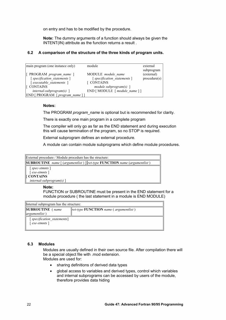
6.2 A comparison of the structure of the three kinds of program units.
main program (one instance only) module external
subprogram [ PROGRAM program_name ]
[ specification_statements ]
[ executable_statements ]
[ CONTAINS
internal-subprogram(s) ]
END [ PROGRAM [ program_name ] ]
MODULE module_name
[ specification_statements ]
[ CONTAINS
module subprogram(s) ]
END [ MODULE [ module_name ] ]
(external)
procedure(s)
Notes:
The PROGRAM program_name is optional but is recommended for clarity.
There is exactly one main program in a complete program
The compiler will only go as far as the END statement and during execution this will cause termination of the program, so no STOP is required.
External subprogram defines an external procedure.
A module can contain module subprograms which define module procedures.
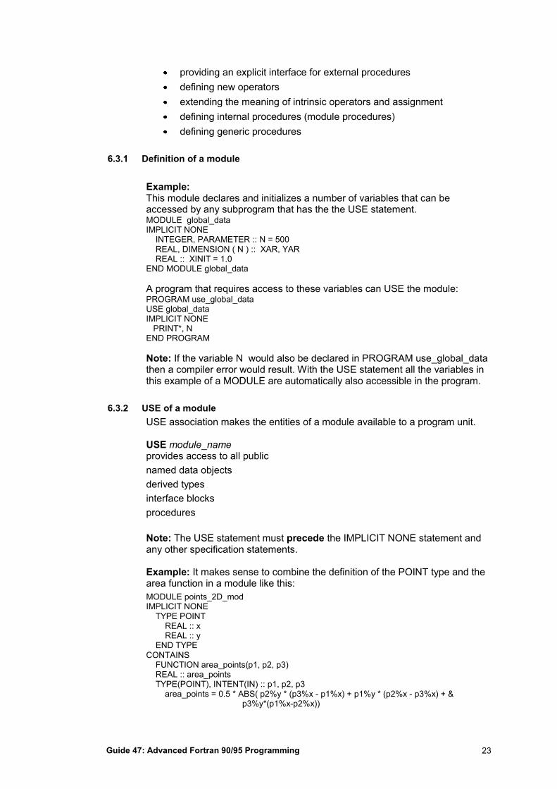
External procedure / Module procedure has the structure:
SUBROUTINE name [ (argumentlist ) ] ret-type FUNCTION name (argumentlist )
[ spec-stmnts ]
[ exe-stmnts ]
[ CONTAINS
internal-subprogram(s) ]
Note: FUNCTION or SUBROUTINE must be present in the END statement for a module procedure ( the last statement in a module is END MODULE)
Internal subprogram has the structure:
SUBROUTINE ( name
argumentlist ) ret-type FUNCTION name ( argumentlist )
[ specification_statements]
[ exe-stmnts ]
6.3 Modules
Modules are usually defined in their own source file. After compilation there will be a special object file with .mod extension. Modules are used for:
sharing definitions of derived data types
global access to variables and derived types, control which variables and internal subprograms can be accessed by users of the module, therefore provides data hiding
Guide 47: Advanced Fortran 90/95 Programming 23
providing an explicit interface for external procedures
defining new operators
extending the meaning of intrinsic operators and assignment
defining internal procedures (module procedures)
defining generic procedures
6.3.1 Definition of a module
Example: This module declares and initializes a number of variables that can be accessed by any subprogram that has the the USE statement. MODULE global_data IMPLICIT NONE INTEGER, PARAMETER :: N = 500 REAL, DIMENSION ( N ) :: XAR, YAR REAL :: XINIT = 1.0 END MODULE global_data
A program that requires access to these variables can USE the module: PROGRAM use_global_data USE global_data IMPLICIT NONE PRINT*, N END PROGRAM
Note: If the variable N would also be declared in PROGRAM use_global_data then a compiler error would result. With the USE statement all the variables in this example of a MODULE are automatically also accessible in the program.
6.3.2 USE of a module
USE association makes the entities of a module available to a program unit. USE module_name provides access to all public
named data objects
derived types
interface blocks
procedures
Note: The USE statement must precede the IMPLICIT NONE statement and any other specification statements. Example: It makes sense to combine the definition of the POINT type and the area function in a module like this:
MODULE points_2D_mod IMPLICIT NONE TYPE POINT REAL :: x REAL :: y END TYPE CONTAINS FUNCTION area_points(p1, p2, p3) REAL :: area_points TYPE(POINT), INTENT(IN) :: p1, p2, p3 area_points = 0.5 * ABS( p2%y * (p3%x - p1%x) + p1%y * (p2%x - p3%x) + & p3%y*(p1%x-p2%x))
Guide 47: Advanced Fortran 90/95 Programming 24
END FUNCTION area_points END MODULE ! To use this module one could write a program like PROGRAM points_2D USE points_2D_mod IMPLICIT NONE TYPE(POINT) :: a, b, c a = POINT(1.0, -2.0) b = POINT(-3.0, 4.0) c = POINT(5.0, -6.0) PRINT*, 'Area is ', area_points(a, b, c) END PROGRAM
6.4 Overloading the build-in operators
Similar to whole array operators where the usual arithmetic operator have been extended to work on arrays, it is possible to extend these operators also to arbitrary data types. For example, it is possible to extend the addition operator ( + ) to variables of the TYPE POINT that were defined in a previous example. Each point in the plane can be considered the endpoint of a vector with begin point in the origin. In that case the + operator for two POINTs could mean the usual vector addition, giving the endpoint of the sum vector. The assignment operator ( = ) can also be extended to arbitrary types, which would be useful in the POINT example to assign the endpoint of the vector sum to another POINT. This mechanism of giving a different meaning to the intrinsic operators is called operator overloading. The compiler can decide from the type of the operands (the context) what definition of the operator is intended. Overloading is done with specific interface blocks. Example: MODULE points_2D_mod IMPLICIT NONE TYPE POINT REAL :: x REAL :: y END TYPE ! overloaded assignment operator (=) INTERFACE ASSIGNMENT (=) ! interface ASSIGNMENT block MODULE PROCEDURE assign END INTERFACE ! overloaded operator (+) INTERFACE OPERATOR (+) ! interface OPERATOR block MODULE PROCEDURE add END INTERFACE CONTAINS SUBROUTINE assign(lhs, rhs) TYPE(POINT), INTENT(OUT) :: lhs TYPE(POINT), INTENT(IN) :: rhs ! here you have to fill in what you want this procedure to do END SUBROUTINE ! overloaded + operator TYPE(POINT) FUNCTION add(pt1, pt2) TYPE(POINT), INTENT(IN) :: pt1, pt2 ! here you have to fill in what you want this procedure to do END FUNCTION END MODULE
Exercise: Copy the above example in a file and fill in the bodies of the assignment and addition operators. The write a main program that declares some points and does some addition and assignment operators. Also add
Guide 47: Advanced Fortran 90/95 Programming 25
some more overloaded operators, e.g. subtraction of two vectors. With what would functionality could you overload the * operator for two POINTs?
6.5 Generic Procedures
Previously it was shown that a generic intrinsic function like SIN can be applied to both scalar and array arguments of any intrinsic type. It is also possible to apply this to user defined procedures, and make them into a single generic name but allowing different types of arguments.
Example: Returning to the example of calculating the area of a triangle in 2D, there were a number of functions available for this purpose but each had a different name, e.g. area_coords(x1, y1, x2, y2, x3, y3), area_points(a, b, c) and area_triangle(triangle) depending on the argument types. In the next example a generic interface block is used to define the generic function area which covers all the different types of arguments, including the derived types. Example: (Continued from previous) MODULE points_2D_mod IMPLICIT NONE TYPE POINT REAL :: x, y
END TYPE ! interface blocks for overloaded assignment and addition operators here ! generic interface for the area function INTERFACE area MODULE PROCEDURE area_coords MODULE PROCEDURE area_points MODULE PROCEDURE area_triangle END INTERFACE CONTAINS ! overloaded functions for assignment and addition operators here REAL FUNCTION area_coords(x1, y1, x2, y2, x3, y3) RESULT(area) REAL, INTENT(IN) :: x1, y1, x2, y2, x3, y3 area = 0.5 * ABS( y2 * (x3 - x1) + y1 * (x2 - x3) + y3*(x1-x2)) END FUNCTION area_coords ! and similar for area_points and area_triangle here END MODULE
6.6 Summary
A module may contain USE statements itself to access other modules.
A module but must not access itself directy or indicrectly through a chain of USE statements.
The standard does not require ordering of modules for compilation. However many compilers require this. Eg if the file mod_a.f90 defines MODULE mod_a and USEs MODULE mod_b, which is defined in mod_b.f90 then often mod_b.f90 has to be compiled before mod_a.f90.
6.7 An extended example
Example 1 PROGRAM points ! in the plane described by x and y coordinates IMPLICIT NONE REAL,EXTERNAL :: area_coords ! a function to calculate the area of a triangle
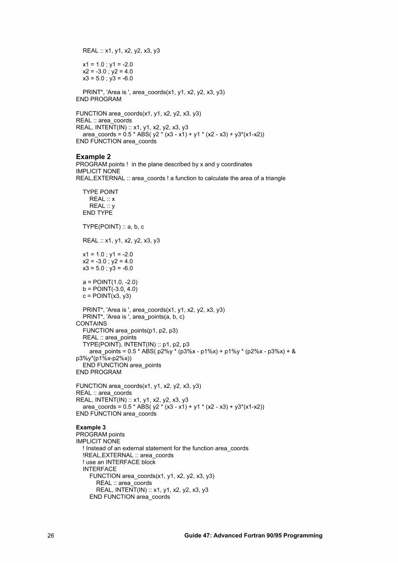
Guide 47: Advanced Fortran 90/95 Programming 26
REAL :: x1, y1, x2, y2, x3, y3 x1 = 1.0 ; y1 = -2.0 x2 = -3.0 ; y2 = 4.0 x3 = 5.0 ; y3 = -6.0 PRINT*, 'Area is ', area_coords(x1, y1, x2, y2, x3, y3) END PROGRAM
FUNCTION area_coords(x1, y1, x2, y2, x3, y3) REAL :: area_coords REAL, INTENT(IN) :: x1, y1, x2, y2, x3, y3 area_coords = 0.5 * ABS( y2 * (x3 - x1) + y1 * (x2 - x3) + y3*(x1-x2)) END FUNCTION area_coords
Example 2 PROGRAM points ! in the plane described by x and y coordinates IMPLICIT NONE REAL,EXTERNAL :: area_coords ! a function to calculate the area of a triangle TYPE POINT REAL :: x REAL :: y END TYPE TYPE(POINT) :: a, b, c REAL :: x1, y1, x2, y2, x3, y3 x1 = 1.0 ; y1 = -2.0 x2 = -3.0 ; y2 = 4.0 x3 = 5.0 ; y3 = -6.0 a = POINT(1.0, -2.0) b = POINT(-3.0, 4.0) c = POINT(x3, y3) PRINT*, 'Area is ', area_coords(x1, y1, x2, y2, x3, y3) PRINT*, 'Area is ', area_points(a, b, c) CONTAINS FUNCTION area_points(p1, p2, p3) REAL :: area_points TYPE(POINT), INTENT(IN) :: p1, p2, p3 area_points = 0.5 * ABS( p2%y * (p3%x - p1%x) + p1%y * (p2%x - p3%x) + & p3%y*(p1%x-p2%x)) END FUNCTION area_points END PROGRAM FUNCTION area_coords(x1, y1, x2, y2, x3, y3) REAL :: area_coords REAL, INTENT(IN) :: x1, y1, x2, y2, x3, y3 area_coords = 0.5 * ABS( y2 * (x3 - x1) + y1 * (x2 - x3) + y3*(x1-x2)) END FUNCTION area_coords Example 3
PROGRAM points IMPLICIT NONE ! Instead of an external statement for the function area_coords !REAL,EXTERNAL :: area_coords ! use an INTERFACE block INTERFACE FUNCTION area_coords(x1, y1, x2, y2, x3, y3) REAL :: area_coords REAL, INTENT(IN) :: x1, y1, x2, y2, x3, y3 END FUNCTION area_coords
Guide 47: Advanced Fortran 90/95 Programming 27
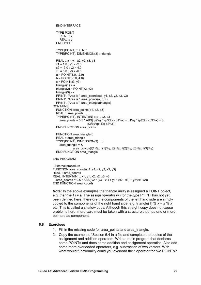
END INTERFACE TYPE POINT REAL :: x REAL :: y END TYPE TYPE(POINT) :: a, b, c TYPE(POINT), DIMENSION(3) :: triangle REAL :: x1, y1, x2, y2, x3, y3 x1 = 1.0 ; y1 = -2.0 x2 = -3.0 ; y2 = 4.0 x3 = 5.0 ; y3 = -6.0 a = POINT(1.0, -2.0) b = POINT(-3.0, 4.0) c = POINT(x3, y3) triangle(1) = a triangle(2) = POINT(x2, y2) triangle(3) = c PRINT*, 'Area is ', area_coords(x1, y1, x2, y2, x3, y3) PRINT*, 'Area is ', area_points(a, b, c) PRINT*, 'Area is ', area_triangle(triangle) CONTAINS FUNCTION area_points(p1, p2, p3) REAL :: area_points TYPE(POINT), INTENT(IN) :: p1, p2, p3 area_points = 0.5 * ABS( p2%y * (p3%x - p1%x) + p1%y * (p2%x - p3%x) + & p3%y*(p1%x-p2%x)) END FUNCTION area_points FUNCTION area_triangle(t) REAL :: area_triangle TYPE(POINT), DIMENSION(3) :: t area_triangle = & area_coords(t(1)%x, t(1)%y, t(2)%x, t(2)%y, t(3)%x, t(3)%y) END FUNCTION area_triangle END PROGRAM ! External procedure FUNCTION area_coords(x1, y1, x2, y2, x3, y3) REAL :: area_coords REAL, INTENT(IN) :: x1, y1, x2, y2, x3, y3 area_coords = 0.5 * ABS( y2 * (x3 - x1) + y1 * (x2 - x3) + y3*(x1-x2)) END FUNCTION area_coords
Note: In the above examples the triangle array is assigned a POINT object, e.g. triangle(1) = a. The assign operator (=) for the type POINT has not yet been defined here, therefore the components of the left hand side are simply copied to the components of the right hand side, e.g. triangle(1) % x = a % x etc. This is called a shallow copy. Although this straight copy does not cause problems here, more care must be taken with a structure that has one or more pointers as component.
6.8 Exercises
1. Fill in the missing code for area_points and area_triangle.
2. Copy the example of Section 6.4 in a file and complete the bodies of the assignment and addition operators. Write a main program that declares some POINTs and does some addition and assignment operatins. Also add some more overloaded operators, e.g. subtraction of two vectors. With what would functionality could you overload the * operator for two POINTs?