advanced foundation engineering prof. kousik deb ...textofvideo.nptel.ac.in/105105039/lec1.pdf ·...

Advanced Foundation Engineering Prof. Kousik Deb

Department of Civil Engineering Indian Institute of Technology, Kharagpur

Lecture - 1

Introduction

Hello. So, today I will start the first lecture on advanced foundation engineering. So, in

this lecture I will be covering different design aspects of various geotechnical structures

like shallow foundation, deep foundation, the retaining wall reinforced retaining wall,

then what would be the soil structure interaction, then how we will design the different

reinforced structure in geotechnical aspect. So, these things will be discussed in this

lecture, and before we discuss about the various design aspects of foundation and the

geotechnical structure foundation of geotechnical structures, then we will start about our

different modules. So, what are the different modules that we will discuss?

(Refer Slide Time: 01:20)

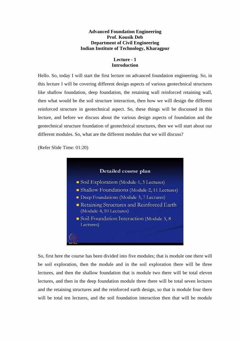
So, first here the course has been divided into five modules; that is module one there will

be soil exploration, then the module and in the soil exploration there will be three

lectures, and then the shallow foundation that is module two there will be total eleven

lectures, and then in the deep foundation module three there will be total seven lectures

and the retaining structures and the reinforced earth design, so that is module four there

will be total ten lectures, and the soil foundation interaction then that will be module

five; there will be total eight lectures. So, including the introduction today’s lecture there

will be total forty lectures in this course.


Now the books that will be that is the reference books and this will be followed in the

lectures. Those are the Arora 2003 which is soil mechanics and foundation engineering

that is the Standard Publishers Distributors. Then Bowles in 1997, then B. M. Das 1983,

then one is Foundation of Soil Dynamics, another is B. M. Das 1999 Principles of

Foundation Engineering, then Hetenyi books that is Beams on Elastic Foundation 1979,

then Koerners books for the Design with Geosynthetics that is 1986.

Then the Kramer books for the Geotechnical Earthquake engineering part because some

part of the earthquake engineering design or design of the retaining wall under

earthquake seismic condition that will also be discussed in this course. So, that part the

reference book is Kramer 2003, then Ranjan and Rao on Basic and Applied Soil

Mechanics 2000 and then Selvadurai that is the Elastic Analysis of Soil Foundation

Interaction 1979 that is the reference books for the soil foundation interaction part, then

N. N. Som and Das 2003 the Theory and Practice of Foundation Design. So, these are

the reference books which will be followed in these lectures.



Now the acknowledgment is given to the professor N.Sivakugan, Associate Professor

and Head, Engineering College, James Cook University, Australia, and Professor B. D.

Manna, Assistant Professor, Department of Civil Engineering, IIT Delhi, and they have

also given some lectures note which will help me to prepare these lectures.


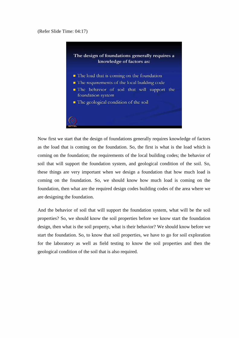
Now first we start that the design of foundations generally requires knowledge of factors

as the load that is coming on the foundation. So, the first is what is the load which is

coming on the foundation; the requirements of the local building codes; the behavior of

soil that will support the foundation system, and geological condition of the soil. So,

these things are very important when we design a foundation that how much load is

coming on the foundation. So, we should know how much load is coming on the

foundation, then what are the required design codes building codes of the area where we

are designing the foundation.

And the behavior of soil that will support the foundation system, what will be the soil

properties? So, we should know the soil properties before we know start the foundation

design, then what is the soil property, what is their behavior? We should know before we

start the foundation. So, to know that soil properties, we have to go for soil exploration

for the laboratory as well as field testing to know the soil properties and then the

geological condition of the soil that is also required.


Next part is if you start the geotechnical properties of the soil, so before we go for the

foundation aspect part, so in the introduction lecture basically I will discuss about some

geotechnical properties and soil properties also that will be required for our design

purpose. So, those are the very important properties. Those things I will discuss in the

introductory lecture, and for the next lecture, lecture two I will start about the different

components of this course of the foundation advanced foundation engineering.

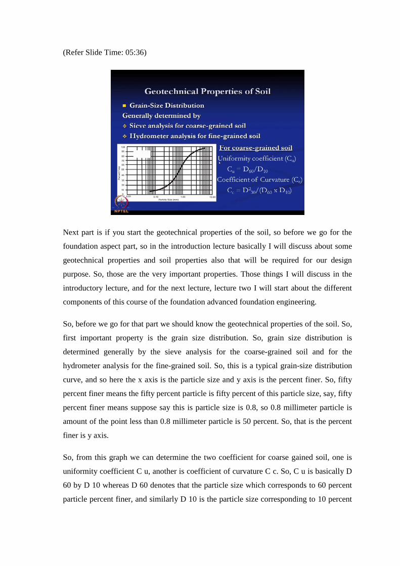
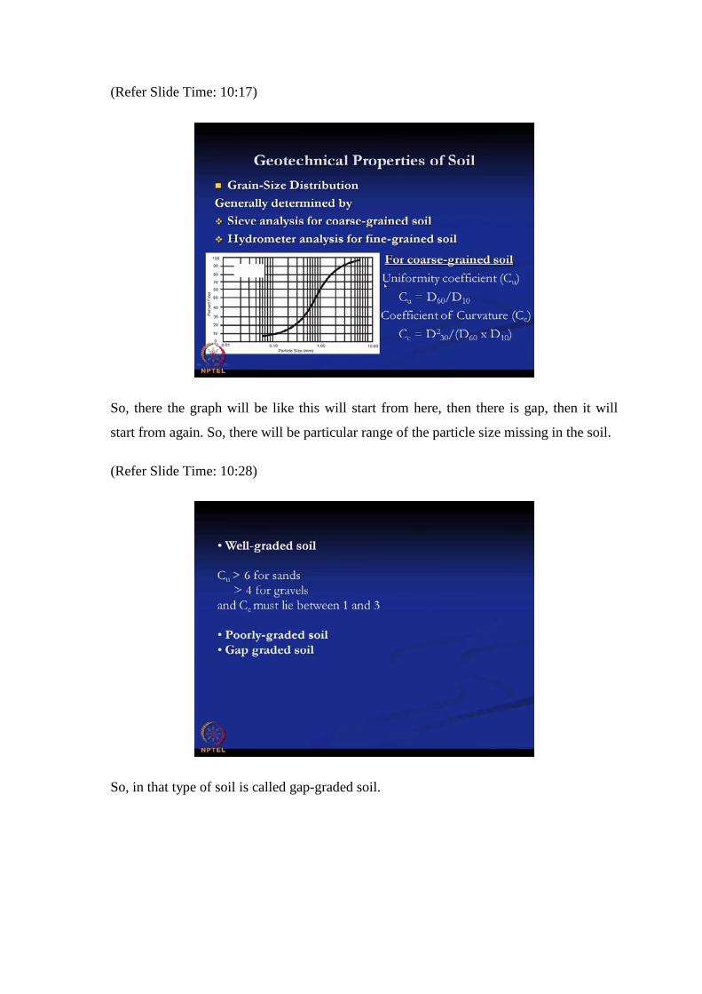
So, before we go for that part we should know the geotechnical properties of the soil. So,

first important property is the grain size distribution. So, grain size distribution is

determined generally by the sieve analysis for the coarse-grained soil and for the

hydrometer analysis for the fine-grained soil. So, this is a typical grain-size distribution

curve, and so here the x axis is the particle size and y axis is the percent finer. So, fifty

percent finer means the fifty percent particle is fifty percent of this particle size, say, fifty

percent finer means suppose say this is particle size is 0.8, so 0.8 millimeter particle is

amount of the point less than 0.8 millimeter particle is 50 percent. So, that is the percent

finer is y axis.

So, from this graph we can determine the two coefficient for coarse gained soil, one is

uniformity coefficient C u, another is coefficient of curvature C c. So, C u is basically D

60 by D 10 whereas D 60 denotes that the particle size which corresponds to 60 percent

particle percent finer, and similarly D 10 is the particle size corresponding to 10 percent

finer. So, from this curve we can determine what is the particle size for 60 percent

particle finer, and what is the particle size for 10 percent finer. So, if we know these two

values from this graph then you will get the uniformity coefficient of the soil. Similarly,

the coefficient of curvatures defined by the D 30 square divided by D 60 into D 10 so

from here you also get the two coefficient.

(Refer Slide Time: 08:24).

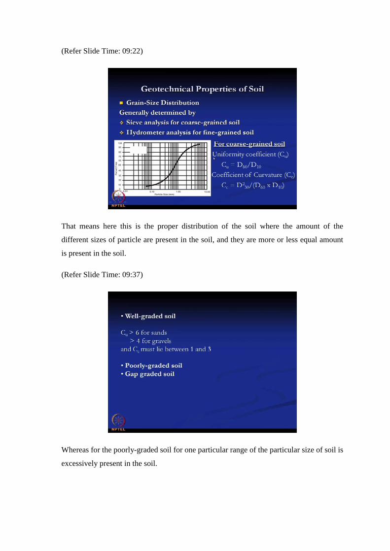
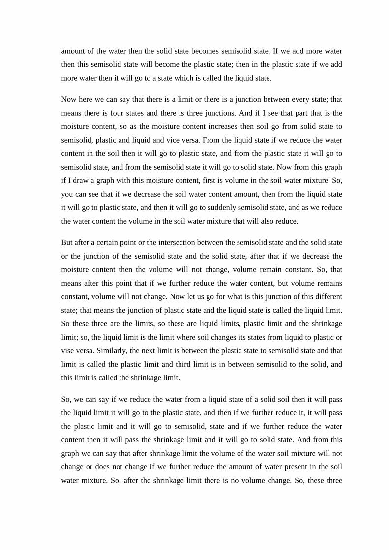
Now the purpose of this two coefficient, so from this two coefficients we can identify

whether this soil is the well-graded soil or soil is the poorly-graded soil. So, well graded

soil if C u is greater than 6 for the sands and is greater than 4 for the gravels and C c

must lie between 1 to 3, then that type of soil is called a well-graded soil. And if it is not

satisfying this condition then that soil is called poorly-graded soil, and third type of soil

is gap graded soil. Now what is well-graded soil, what is poorly-graded soil, what is gap

graded soil. Now well-graded soil that the soil where the different particle size is present

in the soil in almost the equal amount, so that there is proper distribution of the soil.


That means here this is the proper distribution of the soil where the amount of the

different sizes of particle are present in the soil, and they are more or less equal amount

is present in the soil.


Whereas for the poorly-graded soil for one particular range of the particular size of soil is

excessively present in the soil.


So, that means there will be this curve will not be a flat one; it will be a straight one if it

is a poorly-graded soil because one particular range for a particular particle size is

excessively present in the soil; that type of soil is called the poorly-graded soil.


And in gap-graded soil means one particular range of the particles size is missing in the

soil.


So, there the graph will be like this will start from here, then there is gap, then it will

start from again. So, there will be particular range of the particle size missing in the soil.


So, in that type of soil is called gap-graded soil.


Now next one is the weight-volume relationship of the soil. So, as we know that soil is a

three pair system that is air, water and solid. So, from these three pair system we can

determine different soil properties and those properties are very important for the

foundation design. So, if we consider the V a is the volume of the air and V w is the

volume of the water and V s is the volume of the solid. Now here this water and this air

they are present in the voids in between the solids. So, that gives the volume of the water

and volume of the air if we sum these two volume that will give us the volume of the

voids. So, that is V v will be V w plus V a and total volume is v.

Similarly, we can total weight of this soil is considered w, then W s is the weight of the

solid, then W w is the weight of the water and W a is weight of the air generally it is

taken as zero. So, we can neglect the air weight in the soil during the calculation. So,

from this graph we can say that if it is a totally saturated soil that means all the voids are

filled with water then this system become a two phase system; that means the solid and

the water only because that is the fully saturated soil, there will be no air. Now similarly

if the soil is a dry soil completely dry soil then this total void will be filled by the air, so

that means that will also become a two phase system, because all the voids will be filled

by air, there will be no water. So, in that case we have to consider the weight and the

volume accordingly.

Now then the different definition of this one is the void ratio e; void ratio is defined by

volume of void divided by volume of solid. Similarly, porosity is defined as volume of

void divided by total volume. So, we can say here that the void ratio e is the volume of

void divided by volume of solid. So, e value can be greater than 1, but porosity if you

look at the definition of the porosity that is volume of void divided by total volume. So,

the volume of void cannot be greater than the total volume, so the porosity cannot be

greater than one. Now similarly, degree of saturation s which is expressed in percentage

is defined as volume of water divided by volume of voids into 100 because it is

expressed in percentage. Similarly, moisture content w in percentage is weight of water

divided by weight of solid expressed in percentage.


Now the unit weight soil at any water content or any degree of saturation can be written

as because what as I have mentioned that soil can be in the different stage; this can be in

the completely dry stage, it can be in the completely saturated stage, or it can be in some

normal stage, it is not it is partially saturated, this is not completely saturated. So, at

different condition how we will determine the unit weight of the soil, then if we denote

unit weight of the soil is gamma then for gamma bulk or the unit weight at any condition

is given by G s plus S e divided by one plus e into gamma w. So, gamma w is the unit

weight of water; it can be taken as equal to 10 kilo Newton per meter cube. G s is the

specific gravity of the soil and S is the degree of saturation, e is the void ratio.

Now if the soil is completely dry; that means the s is equal to zero, that means saturation

is zero then degree of saturation then the equation of gamma dry will be G s into gamma

w by 1 plus e. So, that is because here s is equal to zero, so this equation becomes this

one for the gamma dry. And then we can write that gamma dry is equal to gamma bulk

divided by 1 plus w; w is the water content of the soil. Bulk density means bulk unit

weight means the unit weight at any condition with any water content, so that is gamma

bulk, gamma bulk is equal to this one. Similarly, gamma sat if I put for the gamma

saturation if it the soil is completely saturated then S value will be equal to 1. So, if in

that case S value is equal to 1 then this equation become this one if it is a completely

saturated soil. So, for the saturated soil this equation become G s plus e gamma w

divided by 1 plus e because in that case S is equal to 1.


The next one is the relative density of the soil. In a granular soil the degree of

compaction in the field can be measured by relative density r d in percentage. So, relative

density can be expressed is e max minus e natural divided by e max minus e min into

100, because it is expressed in terms of percentage where e max is the void ratio of the

soil in the loosest state, and e min is the void ratio in the densest state, and e is the in situ

void ratio on the natural void ratio. So, if we know the e max, e min and e at any

condition then we can determine what is the degree of relative density of the soil at that

situation.


Now next important properties are the Atterberg limits. So, first we will define what are

the Atterberg limits?


So, previous the properties that we have discussed that are the well-graded soil, poorly-

graded soil, gap graded soil, these properties are basically properties for the coarse

grained soil that is for the sand, mille sand, and this is the common thing.


And again relative density is also very important properties for the granular soil or the

course grained soil.


Similarly, the Atterberg limits these limits are very important properties for basically for

the fine grain soil or the clayey soil. So, that means here we can say from this curve the

soil has four different state; that is the solid state, semisolid state, plastic state and liquid

state. Now we can say in this way that if we take a completely dry soil soil-soil that

means that is soil solid soil in the solid state. Now if we add some percentage over some

amount of the water then the solid state becomes semisolid state. If we add more water

then this semisolid state will become the plastic state; then in the plastic state if we add

more water then it will go to a state which is called the liquid state.

Now here we can say that there is a limit or there is a junction between every state; that

means there is four states and there is three junctions. And if I see that part that is the

moisture content, so as the moisture content increases then soil go from solid state to

semisolid, plastic and liquid and vice versa. From the liquid state if we reduce the water

content in the soil then it will go to plastic state, and from the plastic state it will go to

semisolid state, and from the semisolid state it will go to solid state. Now from this graph

if I draw a graph with this moisture content, first is volume in the soil water mixture. So,

you can see that if we decrease the soil water content amount, then from the liquid state

it will go to plastic state, and then it will go to suddenly semisolid state, and as we reduce

the water content the volume in the soil water mixture that will also reduce.

But after a certain point or the intersection between the semisolid state and the solid state

or the junction of the semisolid state and the solid state, after that if we decrease the

moisture content then the volume will not change, volume remain constant. So, that

means after this point that if we further reduce the water content, but volume remains

constant, volume will not change. Now let us go for what is this junction of this different

state; that means the junction of plastic state and the liquid state is called the liquid limit.

So these three are the limits, so these are liquid limits, plastic limit and the shrinkage

limit; so, the liquid limit is the limit where soil changes its states from liquid to plastic or

vise versa. Similarly, the next limit is between the plastic state to semisolid state and that

limit is called the plastic limit and third limit is in between semisolid to the solid, and

this limit is called the shrinkage limit.

So, we can say if we reduce the water from a liquid state of a solid soil then it will pass

the liquid limit it will go to the plastic state, and then if we further reduce it, it will pass

the plastic limit and it will go to semisolid, state and if we further reduce the water

content then it will pass the shrinkage limit and it will go to solid state. And from this

graph we can say that after shrinkage limit the volume of the water soil mixture will not

change or does not change if we further reduce the amount of water present in the soil

water mixture. So, after the shrinkage limit there is no volume change. So, these three

limits are called the Atterberg limits, and these are very important properties for the fine

grain soil.


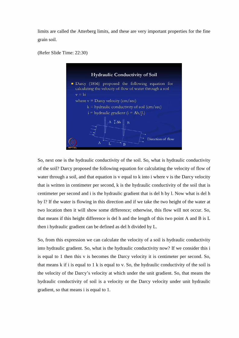
So, next one is the hydraulic conductivity of the soil. So, what is hydraulic conductivity

of the soil? Darcy proposed the following equation for calculating the velocity of flow of

water through a soil, and that equation is v equal to k into i where v is the Darcy velocity

that is written in centimeter per second, k is the hydraulic conductivity of the soil that is

centimeter per second and i is the hydraulic gradient that is del h by l. Now what is del h

by l? If the water is flowing in this direction and if we take the two height of the water at

two location then it will show some difference; otherwise, this flow will not occur. So,

that means if this height difference is del h and the length of this two point A and B is L

then i hydraulic gradient can be defined as del h divided by L.

So, from this expression we can calculate the velocity of a soil is hydraulic conductivity

into hydraulic gradient. So, what is the hydraulic conductivity now? If we consider this i

is equal to 1 then this v is becomes the Darcy velocity it is centimeter per second. So,

that means k if i is equal to 1 k is equal to v. So, the hydraulic conductivity of the soil is

the velocity of the Darcy’s velocity at which under the unit gradient. So, that means the

hydraulic conductivity of soil is a velocity or the Darcy velocity under unit hydraulic

gradient, so that means i is equal to 1.


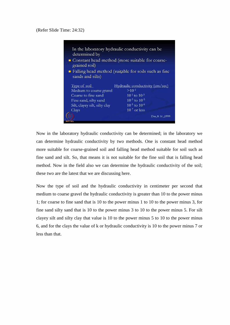
Now in the laboratory hydraulic conductivity can be determined; in the laboratory we

can determine hydraulic conductivity by two methods. One is constant head method

more suitable for coarse-grained soil and falling head method suitable for soil such as

fine sand and silt. So, that means it is not suitable for the fine soil that is falling head

method. Now in the field also we can determine the hydraulic conductivity of the soil;

these two are the latest that we are discussing here.

Now the type of soil and the hydraulic conductivity in centimeter per second that

medium to coarse gravel the hydraulic conductivity is greater than 10 to the power minus

1; for coarse to fine sand that is 10 to the power minus 1 to 10 to the power minus 3, for

fine sand silty sand that is 10 to the power minus 3 to 10 to the power minus 5. For silt

clayey silt and silty clay that value is 10 to the power minus 5 to 10 to the power minus

6, and for the clays the value of k or hydraulic conductivity is 10 to the power minus 7 or

less than that.


So, next concept or the next thing is the effective stress concept. Now what is effective

stress? Now effective stress can be defined as the total stress minus the pore water

pressure. Now where sigma dash is the vertical effective stress and sigma is the vertical

total stress, u is the pore water pressure. So, that means when we apply weight or the

load on a soil stress on a soil, initially that stress this stress is taken by the initial time is

taken by the water. And now if we do not permit any flow of the water that means this

stresses will be taken by the water initial stresses. Now if we permit the water to flow

then gradually this water will flow, and the stress which was taken by the water initially

will be transferred to the soil skeleton.

So, now as time progresses this water goes out then this stresses will be transferred to the

soil skeleton. Now soil will take the stress in that fashion. So, that means when the soil is

totally dry; that means there is more water. Now if we apply the stress on a soil water

system then the stress will be taken by the water if we apply the stress on this condition;

that means this water pore water pressure will be developed. Now if the soil is totally dry

that mean no pore water pressure will be developed in that case u is zero, in that

condition the effective stress will be equal to the total stress. So, that means if u is the

dry condition u is zero that means the sigma dash is equal to sigma and that means dry

means there is no water present in the soil.


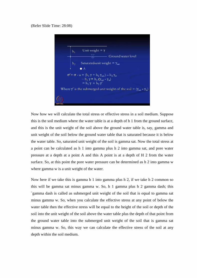
Now how we will calculate the total stress or effective stress in a soil medium. Suppose

this is the soil medium where the water table is at a depth of h 1 from the ground surface,

and this is the unit weight of the soil above the ground water table is, say, gamma and

unit weight of the soil below the ground water table that is saturated because it is below

the water table. So, saturated unit weight of the soil is gamma sat. Now the total stress at

a point can be calculated as h 1 into gamma plus h 2 into gamma sat, and pore water

pressure at a depth at a point A and this A point is at a depth of H 2 from the water

surface. So, at this point the pore water pressure can be determined as h 2 into gamma w

where gamma w is a unit weight of the water.

Now here if we take this is gamma h 1 into gamma plus h 2, if we take h 2 common so

this will be gamma sat minus gamma w. So, h 1 gamma plus h 2 gamma dash; this

`gamma dash is called as submerged unit weight of the soil that is equal to gamma sat

minus gamma w. So, when you calculate the effective stress at any point of below the

water table then the effective stress will be equal to the height of the soil or depth of the

soil into the unit weight of the soil above the water table plus the depth of that point from

the ground water table into the submerged unit weight of the soil that is gamma sat

minus gamma w. So, this way we can calculate the effective stress of the soil at any

depth within the soil medium.


The next thing that I will discuss about the consolidation, consolidation is also very

important properties for the fine grained soil. Now as I have mentioned that soil voids

are filled by either air or water or both. So, if we want to remove this voids, there are

basically two methods by which we can remove this voids; one is compaction another is

consolidation. So, the major difference between these two methods that by compaction

we can remove the air voids but by consolidation we can remove the water voids; so

there are other differences also there based on this two methods, but this is the major

difference. So, here consolidation means we can remove the water voids or water present

with in the soil pores.

So, now this consolidation once we have done the consolidation, this consolidation can

be done in the laboratory and there are some properties which are very important for our

foundation design basically for the settlement because consolidation is very important

properties for the fine grained soil or the clayey soil, because in the sand grained soil

permeability of the soil is very high. So, once we apply the load all the soil or the water

can dissipate within very short duration of the time. So, long term settlement all the

settlement that we will get for the coarse grained soil is the immediate settlement. The

long time settlement is very negligible in case of coarse grained soil, but for the fine

grained soil likely where the permeability is very low.

So, once we apply the load there will be very negligible amount of the immediate

settlement all that depending upon the type of clay, but the most of the settlement will

come because of the consolidation because as time progresses the water will dissipate

from the clayey soil slowly slowly, and then the settlement will occur. So, that is the time

dependent phenomenon and it will take the long time to complete the total settlement.

So, that is why consolidation and that settlement is called the consolidation settlement,

and that consolidation settlement is very important properties for a fine grained soil

during the foundation design.

So, in the consolidation after what we can do we can apply the load on a soil sample or

apply the pressure on a soil sample, and we can determine what is the amount of void in

the soil or we can determine the void ratio. So, it is expected as we apply the more

pressure the void ratio will decrease. So, here a typical consolidation I mean void ratio

versus log p, p means the pressure graph is presented. Now this pressure is plotted in the

logarithm scale and void ratio in the normal scale. So, this is log p. So, here we can see

as we apply the more pressure the void ratio decreases. This is the loading curve and this

is the unloading curve, so once we remove the pressure so there will be some rebound of

the soil voids. So, it will further go up.

Now here the slope we can determine the compression index that is the slope of this

loading curve. So, this slope of loading curve so the compression index C c is equal to e

1 minus e 2 divided by log p 2 minus log p 1. Now e 1 is the void ratio corresponding to

pressure p 1, and e 2 is the void ratio corresponding to pressure p 2. So, this is basically

C c is the slope of this loading path. Now according to Skempton we can determine the C

c also that is 0.009, LL is the liquid limit minus 10; in this way also we can determine

what is the value of C c.


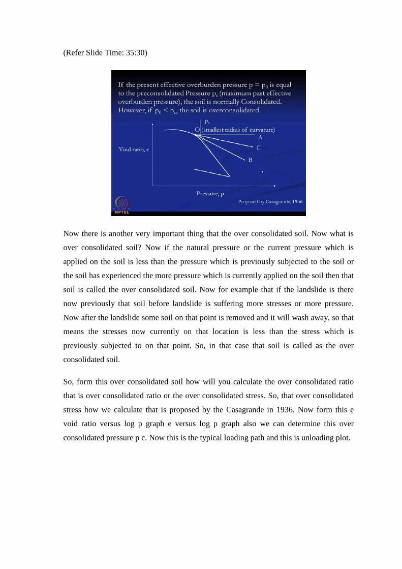
Now there is another very important thing that the over consolidated soil. Now what is

over consolidated soil? Now if the natural pressure or the current pressure which is

applied on the soil is less than the pressure which is previously subjected to the soil or

the soil has experienced the more pressure which is currently applied on the soil then that

soil is called the over consolidated soil. Now for example that if the landslide is there

now previously that soil before landslide is suffering more stresses or more pressure.

Now after the landslide some soil on that point is removed and it will wash away, so that

means the stresses now currently on that location is less than the stress which is

previously subjected to on that point. So, in that case that soil is called as the over

consolidated soil.

So, form this over consolidated soil how will you calculate the over consolidated ratio

that is over consolidated ratio or the over consolidated stress. So, that over consolidated

stress how we calculate that is proposed by the Casagrande in 1936. Now form this e

void ratio versus log p graph e versus log p graph also we can determine this over

consolidated pressure p c. Now this is the typical loading path and this is unloading plot.


Similar to this graph is loading and unloading path.


Now form this loading path you have to identify a point to which as the smallest radius

of curvature. Now form here, here we can get the different curvature and we will get a

point O here which has the smallest radius of curvature. Now once you select the point O

then we can draw a line OA which is parallel to x axis. Now from first select the point to

which has the smallest radius of curvature. Now from point O draw a line OA which is

parallel to pressure p x axis.

Now form this point A draw a line OB such that this OB is a tangent at O. So, draw a

line OB such that OB is a tangent at O; then draw another line OC such that it bisects this

angle AOB, and once we get the OC line the next step is to extend this straight portion of

the loading curve. Now extend this state portion of the loading curve, and identify the

point where the straight portion of the loading curve and this bisection curve intersects.

Now identify that point and pressure corresponding to that point is called the over

consolidated pressure or maximum past effective overburden pressure.

So, that the present if the present, so this way we can determine the P c which is

maximum past effective overburden pressure; now if present effective overburden

pressure p 0 is equal to preconsolidated pressure P c then the soil is called normally

consolidated soil; that means the present effective overburden pressure is equal to this

preconsolidated maximum past effective overburden pressure p c, then that soil is called

normally consolidated soil. Now if this p 0 that means the present effective overburden

pressure is less than the P c or the past effective overburden pressure as I have mentioned

then that soil is called over consolidated soil. So, this way from this log e versus log p

curve also we can determine the p c value.


Now how we will calculate the consolidation settlement of a soil, because as I have

mention that the foundation design this settlement calculation is very important issue for

the clayey soil. Now here how we will calculate the settlement for the consolidation

settlement? So, there is two type of soil we have considered; one is normally

consolidated clay, another is over consolidated clay. So, now in the normally

consolidated clay this is the typical loading path that we will consider that is the straight

portion we can consider for the normally consolidated clay. And here that slope of this

curve will give us the C c as I have mentioned the slope of this curve the composition

index, so that means this is the difference between stress is del p p 0 and p 0 plus del p

that is the difference between stress, and because of this stress difference this is the

difference between the void ratio del E, and as expected as we increase the pressure I the

void ratio will decrease.

So, similarly then similar curve we can draw for the over consolidated clay, for the over

consolidated clay so this is the typical curve log e versus log p curve. And here this is the

point where we got the p c value, and then we will locate this point, how we will get this

P c value we have already explained, and then there is two parts. One is this one whose

slope will give us the C c composition index and another is this part this above this P c

value portion that is the C s, and here also P 0 plus del p there will be the del e and here

also p 0 plus del p that portion there also we will get that. So, that means here we will get

the del p del E i and del E 2. So, there basically we have two different portions.


Now for the normally consolidated clay how we will calculate that for the settlement S is

C c 1 plus e 0 into H log p 0 plus del p divided by p 0.


So, this is the settlement calculation for typical this portion.


Now where C c is the compression index, e 0 is the initial void ratio, H is the thickness

of the soil layer for which we are determining the settlement, and p 0 is the initial applied

stress and del p is the stress or additional stress; that means for example, the p 0 is equal

to effective overburden pressure, and del p is the additional stress due to the applied

external load on the foundation. So, later on when you talk about the foundation

settlement calculation, you will show how this p 0 and del p 0 can be calculated. So, that

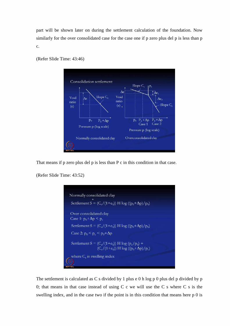
part will be shown later on during the settlement calculation of the foundation. Now

similarly for the over consolidated case for the case one if p zero plus del p is less than p

c.


That means if p zero plus del p is less than P c in this condition in that case.


The settlement is calculated as C s divided by 1 plus e 0 h log p 0 plus del p divided by p

0; that means in that case instead of using C c we will use the C s where C s is the

swelling index, and in the case two if the point is in this condition that means here p 0 is

less than p c, p 0 plus del p is greater than p c. In that condition settlement we can

calculate the c s plus 1 plus e 0 into h log p c divided by p 0 plus C c divided by 1 plus e

0 into h log p 0 plus del p divided by p c. So, in these two conditions how we can

determine the consolidation settlement? So, one is normally consolidated soil, this is the

expression. If it is over consolidated soil if case one this is the expression; if it is case

two this is the expression.


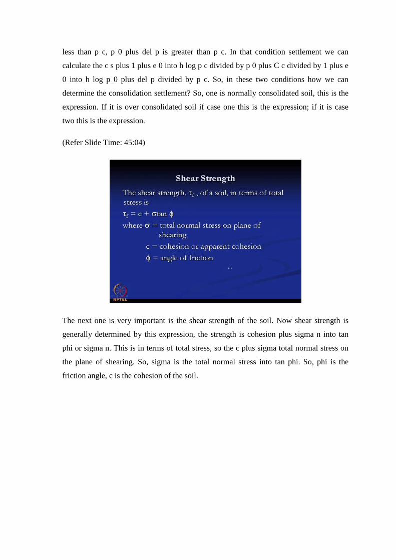
The next one is very important is the shear strength of the soil. Now shear strength is

generally determined by this expression, the strength is cohesion plus sigma n into tan

phi or sigma n. This is in terms of total stress, so the c plus sigma total normal stress on

the plane of shearing. So, sigma is the total normal stress into tan phi. So, phi is the

friction angle, c is the cohesion of the soil.


Now these things we can draw which is the Mohr-Coulomb failure criteria or Mohr-

Coulomb failure envelope is there. So, this is the envelope, and this is the sigma axis

normal stress axis and this is the shear stress axis. Now if any Mohr-Coulomb touches a

Mohr circle touches this envelope; that means that failure will occur and anything so that

means here this expression shear strength expression is c plus sigma into tan phi, phi we

can determine by tan phi is the slope of this angle. So, if we know the slope of this angle

we can determine the slope of this line; if we know the slope of this line you can

determine the angle phi here also.

So, tau f is the maximum shear stress in soil that can take without any failure under

normal stress sigma. Now this is the same expression we can write in terms of effective

stress. So, in terms of effective stress this will be c bar effective coefficient then the

sigma dash or tau phi dash. So, sigma dash will be sigma minus u, u is the pore water

pressure and similar envelope you can determine but only this in terms of effective

stress. So, tau f is the maximum shear stress the soil can take without failure under

normal effective stress of sigma bar.


Now these properties, so that means here we can see the c and phi these are the strength

properties of the soil. So, those are very important things for the and this c and phi these

two parameters very important for the foundation design for the foundation bearing

capacity design; that means how much amount of load foundation can carry this, we can

determine this based on these two parameters. So, these two parameters we have to

determine; in the laboratory we can determine these two parameters in different by this

different test. One is direct shear test generally for the sand then triaxial test conducted

on sands and clay both, and these are three types of test depending upon the drainage

condition, depending that is the consolidated-drained test CD, consolidated-undrained

test, unconsolidated-undrained test UU.

So, depending upon whether it is a consolidated or unconsolidated drained or undrained

these are three types of triaxial test. Another test which is conducted is unconfined

compression strength. This is suitable for the soil whose saturated clay; that means phi

value is equal to zero; that means the shear strength of the saturated clay can be

calculated for this type of test tau f equal to CU. CU is the undrained coefficient of the

soil and here if the unconfined compression strength is q u then if you divide it by 2; that

means there you will get the CU. So, half of the QU will give you the CU. So, that is the

unconfined compressive stress divided by 2 that will give us the CU for unconfined

compressive strength test.


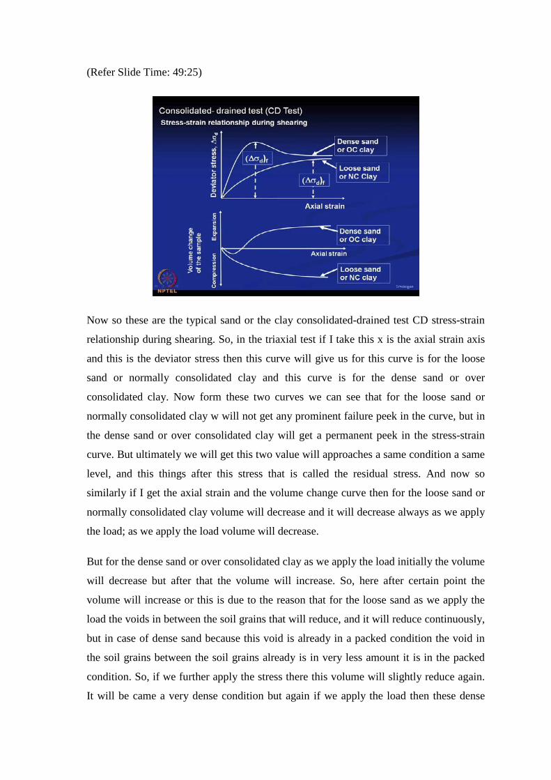
Now so these are the typical sand or the clay consolidated-drained test CD stress-strain

relationship during shearing. So, in the triaxial test if I take this x is the axial strain axis

and this is the deviator stress then this curve will give us for this curve is for the loose

sand or normally consolidated clay and this curve is for the dense sand or over

consolidated clay. Now form these two curves we can see that for the loose sand or

normally consolidated clay w will not get any prominent failure peek in the curve, but in

the dense sand or over consolidated clay will get a permanent peek in the stress-strain

curve. But ultimately we will get this two value will approaches a same condition a same

level, and this things after this stress that is called the residual stress. And now so

similarly if I get the axial strain and the volume change curve then for the loose sand or

normally consolidated clay volume will decrease and it will decrease always as we apply

the load; as we apply the load volume will decrease.

But for the dense sand or over consolidated clay as we apply the load initially the volume

will decrease but after that the volume will increase. So, here after certain point the

volume will increase or this is due to the reason that for the loose sand as we apply the

load the voids in between the soil grains that will reduce, and it will reduce continuously,

but in case of dense sand because this void is already in a packed condition the void in

the soil grains between the soil grains already is in very less amount it is in the packed

condition. So, if we further apply the stress there this volume will slightly reduce again.

It will be came a very dense condition but again if we apply the load then these dense

conditions will become a loose condition; that means the loose means the void in

between the soil particles that will increase. So, once it becomes very dense then after

that if we apply the stress it is become again the force volume will increase. So, that is

why this volume will change for the dense sand.



For similar curve we will get for the direct shear stress also this is for the dense sand and

this is for the loose sand. Hence we will have volume versus shear strength. So, this is

the shear displacement and shear stress and previous curve was axial stress and deviatory

stress axial strain and deviatory stress but the similar nature of the curve we will get.

Now so this in the successive lectures you will get some corrections required so that in

the different lectures. So, this is the additional slide that is put here. So, in the lecture 3 in

this time 57.16 minutes it is recorded the soil as soil rather that it should be in-situ test

replaced this reference by this difference. So, in lecture 4 at this 19.20 minute replace

refracted by refracted rays, lecture nine 52.40 minute it is foundation on layered soil

instead of raft foundation. In lecture 15 unit of unit weight is kilo Newton per meter cube

not kilo Newton per meter square, lecture 29 it tells to discuss about the braced cut but

not discussed there; at two minute it is reinforced found instead of RCC foundation as

said. In lecture 30 modulus of subgrade reaction is stress per unit deflection and not

stress per unit per area.


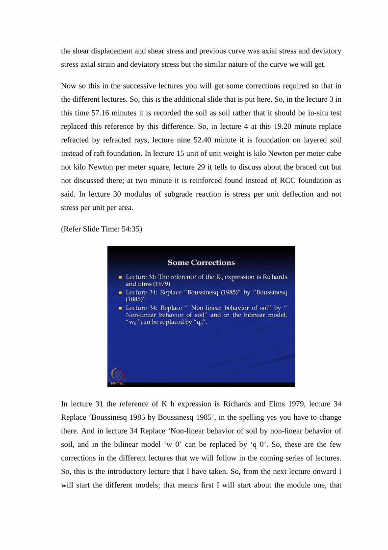
In lecture 31 the reference of K h expression is Richards and Elms 1979, lecture 34

Replace ‘Boussinesq 1985 by Boussinesq 1985’, in the spelling yes you have to change

there. And in lecture 34 Replace ‘Non-linear behavior of soil by non-linear behavior of

soil, and in the bilinear model ‘w 0’ can be replaced by ‘q 0’. So, these are the few

corrections in the different lectures that we will follow in the coming series of lectures.

So, this is the introductory lecture that I have taken. So, from the next lecture onward I

will start the different models; that means first I will start about the module one, that

means the soil exploration, then we will start module two, three, four and five. So, in the

next class I will start about the soil exploration.

Thank you.

advanced foundation engineering prof. kousik deb ...textofvideo.nptel.ac.in/105105039/lec1.pdf ·...

Documents