Advanced Heat Integration Tool for

Simulation-based Optimization Framework

Yang Chen a,b, John Eslick a,b, Ignacio Grossmann a, David Miller b

a. Dept. of Chemical Engineering, Carnegie Mellon University

b. National Energy Technology Laboratory

November 18, 2014

2

+ Treats simulation as black box (does not require mathematical

details of model)

+ Does not require simplification of the process model

+ Readily adapted for parallel computing

− Not well suited for problems with many variables such as heat

integration, and superstructure optimization

Simulation-Based Optimization

Easy to implement

Goal: Develop a simulation-based optimization

framework with heat integration for large-scale high-

fidelity process models.

High-fidelity models applied

Computational time reduced

Heat integration is a separate module linked to

simulation-based optimization algorithm

3

Simulation-Based Optimization with Heat Integration

heater

cold stream

hot stream

cooler

Process Simulator(s)

hot stream

cold stream

heat exchanger

heater (with utility)

cooler (with utility)

Heat Integration Tool

Optimization Solver

0x

xx

)( s.t.

)( min

g

f

Optimal values for

Decision Variables Process Results

Initial Inputs

Optimal Outputs

Hot/Cold Stream

Information

e.g., Flow rates,

Temperatures, Enthalpy, …

Heat Integration Results:

Minimum utility cost (or consumption)

Minimum heat exchanger area

Simultaneous

process optimization

and heat integration

based on rigorous

process simulations

are achieved in this

framework

Parameters

Physical

Properties

Aspen Plus,

ACM,

gPROMS

GAMS

LP Models

DFO

4

• LP Transshipment Model

Minimum Utility Cost (Consumption)

Wn

W

nn

Sm

S

mm QcQcZ min

k

H

ik

Wn

ink

Cj

ijkkiik HiQQQRRkk

s.t. 1,

k

S

m

Cj

mjkkmmk SmQQRRk

01,

k

C

jk

Sm

mjk

Hi

ijk CjQQQkk

KkWnQQ k

W

n

Hi

ink

k

,...,1 0

0 , , , , , , W

n

S

minkmjkijkmkik QQQQQRR 00 iKi RR

QS heat load of hot utility

QW heat load of cold utility

QH heat load of hot process stream

QC heat load of cold process stream

Q exchange of heat

R heat residual

c unit cost of utility

k temperature interval

i hot process stream

j cold process stream

m hot utility

n cold utility

‒ Heat loads of the streams are calculated directly from the total change of

enthalpy from the simulation results.

‒ Assumption: Constant heat capacity flowrates (FCps) for streams.

Papoulias SA, Grossmann IE. Comput. & Chem. Eng. 1983;7(6):707-721.

5

• A process stream with phase change

Stream with Variable FCp

A mixture stream of CO2 and H2O (CO2: 40%, H2O: 60%; 1kmol/hr; 1 bar)

20

40

60

80

100

120

140

160

0 5 10 15 20 25 30 35

Tem

pera

ture

(C

)

Heat Load (MJ/hr)

6

Problems with Constant FCps

20

40

60

80

100

120

140

160

0 5 10 15 20 25 30 35

Tem

pera

ture

(C

)

Heat Load (MJ/hr)

• Overestimate the heat recovery

• Infeasible heat exchanger network design

7

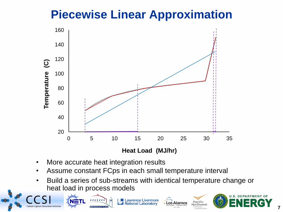
Piecewise Linear Approximation

20

40

60

80

100

120

140

160

0 5 10 15 20 25 30 35

Tem

pera

ture

(C

)

Heat Load (MJ/hr)

• More accurate heat integration results

• Assume constant FCps in each small temperature interval

• Build a series of sub-streams with identical temperature change or heat load in process models

8

• LP Area Targeting Model (Modified from LP

Transportation Model)

Minimum Heat Exchanger Area

k lHi Cj ji

jlikK

k

K

l k,l hh

q ,

1 1

LMTD

1

Ft

1 min

KkHiQq k

K

kl

H

ik

Cj

jlik

l

,...,1 s.t. ,

QH heat load of hot stream

QC heat load of cold stream

q exchange of heat

Ft correction factor for a

non-countercurrent flow

h stream film heat transfer

coefficient

LMTD logarithmic-mean

temperature difference

k temperature interval

l temperature interval

i hot stream

j cold stream

KlCjQq l

l

k

C

jl

Hi

jlik

k

,...,1 1

,

‒ Temperature interval should be smaller than the minimum utility problem for

accurate area targets.

‒ Number of temperature intervals: accurate results vs. CPU times.

‒ Double-temperature approach: HRAT & EMAT.

Jezowski JM, Shethna HK, Castillo FJL. Ind. Eng. Chem. Res. 2003;42(8):1723-1730.

9

Implementation - Graphical User Interface

Framework for Optimization and Quantification of Uncertainty and Sensitivity (FOQUS)

Run a Simulation

Add a Edge

Add a Node

Stop a Simulation

Select a Node/Edge

Delete a Node/Edge

Load Default Inputs

Determine Tear Streams

Flowsheet Settings

Center Flowsheet View

Home Screen

(load/save

problems)

Flowsheet Editor

Uncertainty Quantification Tool

Optimization Tool Surrogate Model Tool

Help Documents

Node (a model run on

process simulators or

Python code)

Edge (information

transfer between

models)

Heat Integration Node (where

heat integration is performed)

10

Simulation Model (1)

Input Variables

ACM Simulation Model

11

Simulation Model (2)

Output Variables

12

Heat Integration Tool (1)

Heat Integration Inputs

Heat Integration Model (GAMS)

EMAT (Exchanger Minimum

Approach Temperature)

HRAT (Heat Recovery

Approach Temperature)

13

Heat Integration Tool (2)

Utility Consumptions

Heat Integration Outputs

Minimum Utility Cost

Minimum Heat Exchanger Area

14

Optimization Solver

Solver Selection

Description of Current Solver

Solver Option Settings

15

Optimization Problem Setting

Run Optimization

Select Decision Variables

Inequality Constraint (Python expression enforced with penalty)

Objective Function (Python expression)

Variable Scaling Method

(Input variables are scaled to be 0 at min and 10 at max)

Min/Max Bounds

Current Value (Initial Guess)

16

Case Study – A Power Plant with CO2 Capture

17

Problem Statement

Objective Function: Maximizing Net efficiency

Constraint: CO2 removal ratio ≥ 90%

Flowsheet evaluation (via process simulators)

Minimum utility and area target (via heat integration tool)

Decision Variables (23): Bed length, diameter, sorbent and steam feed

rates, temperatures

Heat Integration Node

(GAMS)

BFB Adsorber and

Regenerator Model (ACM)

Compressor Model

(ACM)

Total Electricity

Consumption Calculation

(Python)

Steam Cycle Model and

Net Efficiency Calculation

(Python)

18

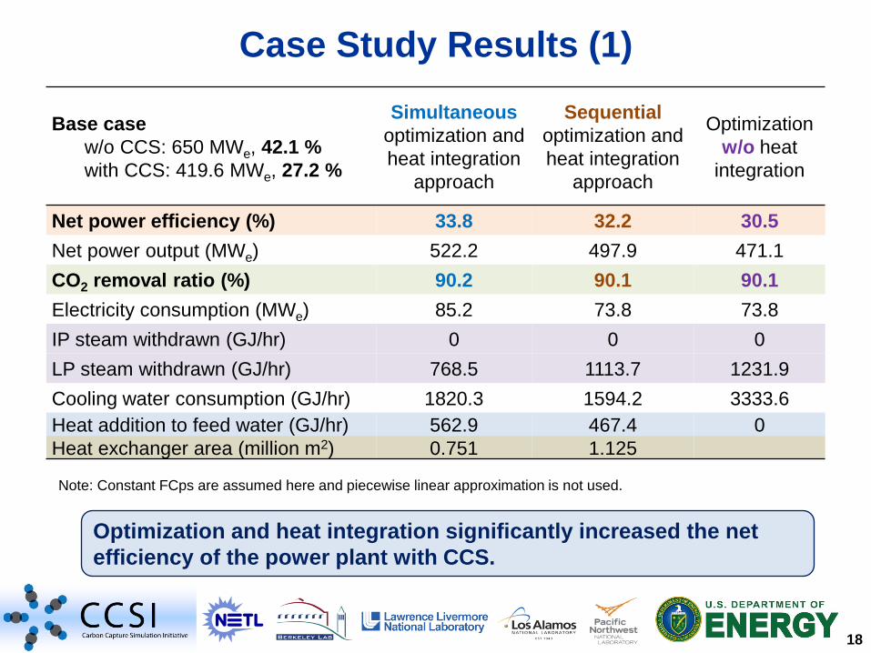
Case Study Results (1)

Optimization and heat integration significantly increased the net

efficiency of the power plant with CCS.

Base case

w/o CCS: 650 MWe, 42.1 %

with CCS: 419.6 MWe, 27.2 %

Simultaneous

optimization and

heat integration

approach

Sequential

optimization and

heat integration

approach

Optimization

w/o heat

integration

Net power efficiency (%) 33.8 32.2 30.5

Net power output (MWe) 522.2 497.9 471.1

CO2 removal ratio (%) 90.2 90.1 90.1

Electricity consumption (MWe) 85.2 73.8 73.8

IP steam withdrawn (GJ/hr) 0 0 0

LP steam withdrawn (GJ/hr) 768.5 1113.7 1231.9

Cooling water consumption (GJ/hr) 1820.3 1594.2 3333.6

Heat addition to feed water (GJ/hr) 562.9 467.4 0

Heat exchanger area (million m2) 0.751 1.125

Note: Constant FCps are assumed here and piecewise linear approximation is not used.

19

Case Study Results (2)

Base case

w/o CCS: 650 MWe, 42.1 %

with CCS: 419.6 MWe, 27.2 %

Heat integration

with constant

FCps

Heat integration

with variable

FCps

(5 segments)

w/o heat

integration

Net power efficiency (%) 33.8 31.9 30.5

Net power output (MWe) 522.2 493.4 471.1

CO2 removal ratio (%) 90.2 90.0 90.1

Electricity consumption (MWe) 85.2 72.0 73.8

IP steam withdrawn (GJ/hr) 0 0 0

LP steam withdrawn (GJ/hr) 768.5 1089.7 1231.9

Cooling water consumption (GJ/hr) 1820.3 1700.8 3333.6

Heat addition to feed water (MWth) 562.9 313.9 0

Heat exchanger area (million m2) 0.751 0.923

After considering variable FCps and using piecewise linear approximation of

the composite curve, the net efficiency is somewhat decreased but the

obtained results become much more realistic.

20

• Simulation-based optimization framework with heat

integration is a suitable tool for optimization of large-scale

high-fidelity process models.

• This framework can be easily implemented in the

software FOQUS.

• Performance of power plant with CCS can be significantly

increased by simultaneous optimization and heat

integration.

• More accurate heat integration results are obtained by

using piecewise linear approximation for the composite

curve of process streams.

Conclusions

21

Jim Leek (LLNL)

Josh Boverhof (LBNL)

Juan Morinelly, Melissa Daly (CMU)

DOE: Carbon Capture Simulation Initiative (CCSI)

Acknowledgement

Disclaimer

This presentation was prepared as an account of work sponsored by an agency of the United

States Government under the Department of Energy. Neither the United States Government

nor any agency thereof, nor any of their employees, makes any warranty, express or implied,

or assumes any legal liability or responsibility for the accuracy, completeness, or usefulness of

any information, apparatus, product, or process disclosed, or represents that its use would not

infringe privately owned rights. Reference herein to any specific commercial product, process,

or service by trade name, trademark, manufacturer, or otherwise does not necessarily

constitute or imply its endorsement, recommendation, or favoring by the United States

Government or any agency thereof. The views and opinions of authors expressed herein do

not necessarily state or reflect those of the United States Government or any agency thereof.