advanced machine learning lecture 20 - computer vision · restricted boltzmann machines (rbm)...
TRANSCRIPT
Perc
eptu
al
and S
enso
ry A
ugm
ente
d C
om
puti
ng
Ad
van
ced
Mach
ine L
earn
ing
Winter’15
Advanced Machine Learning
Lecture 20
Restricted Boltzmann Machines
01.02.2016
Bastian Leibe
RWTH Aachen
http://www.vision.rwth-aachen.de/
TexPoint fonts used in EMF.
Read the TexPoint manual before you delete this box.: AAAAAAAAAAAAAAAAAAAAAAAAAAAAAAAA
Perc
eptu
al
and S
enso
ry A
ugm
ente
d C
om
puti
ng
Ad
van
ced
Mach
ine L
earn
ing
Winter’15
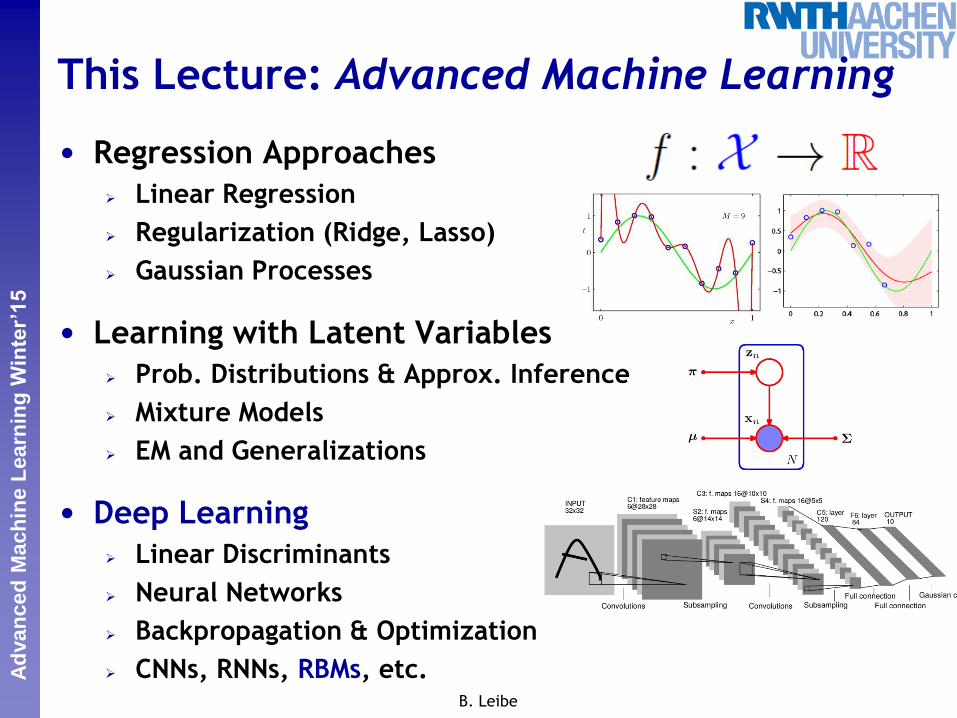
This Lecture: Advanced Machine Learning
• Regression Approaches
Linear Regression
Regularization (Ridge, Lasso)
Gaussian Processes
• Learning with Latent Variables
Prob. Distributions & Approx. Inference
Mixture Models
EM and Generalizations
• Deep Learning
Linear Discriminants
Neural Networks
Backpropagation & Optimization
CNNs, RNNs, RBMs, etc. B. Leibe
Perc
eptu
al
and S
enso
ry A
ugm
ente
d C
om
puti
ng
Ad
van
ced
Mach
ine L
earn
ing
Winter’15
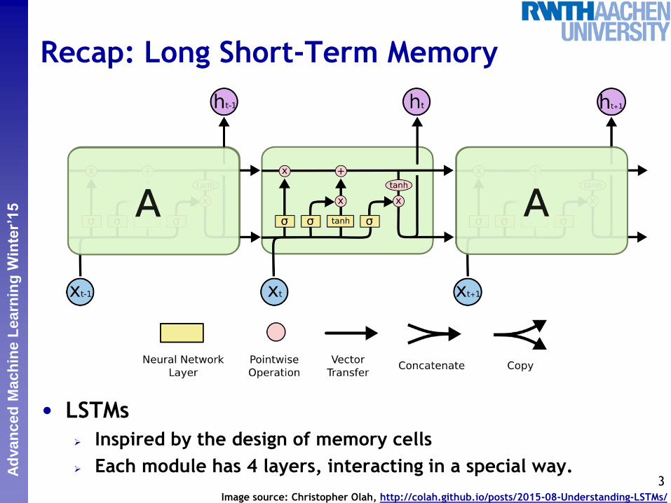
Recap: Long Short-Term Memory
• LSTMs
Inspired by the design of memory cells
Each module has 4 layers, interacting in a special way. 3
Image source: Christopher Olah, http://colah.github.io/posts/2015-08-Understanding-LSTMs/
Perc
eptu
al
and S
enso
ry A
ugm
ente
d C
om
puti
ng
Ad
van
ced
Mach
ine L
earn
ing
Winter’15
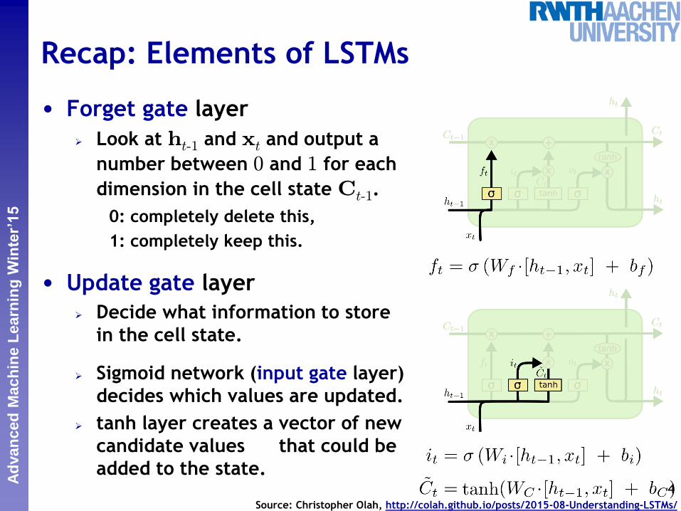
Recap: Elements of LSTMs
• Forget gate layer
Look at ht-1 and xt and output a
number between 0 and 1 for each
dimension in the cell state Ct-1.
0: completely delete this,
1: completely keep this.
• Update gate layer
Decide what information to store
in the cell state.
Sigmoid network (input gate layer)
decides which values are updated.
tanh layer creates a vector of new
candidate values that could be
added to the state.
4 Source: Christopher Olah, http://colah.github.io/posts/2015-08-Understanding-LSTMs/
Perc
eptu
al
and S
enso
ry A
ugm
ente
d C
om
puti
ng
Ad
van
ced
Mach
ine L
earn
ing
Winter’15
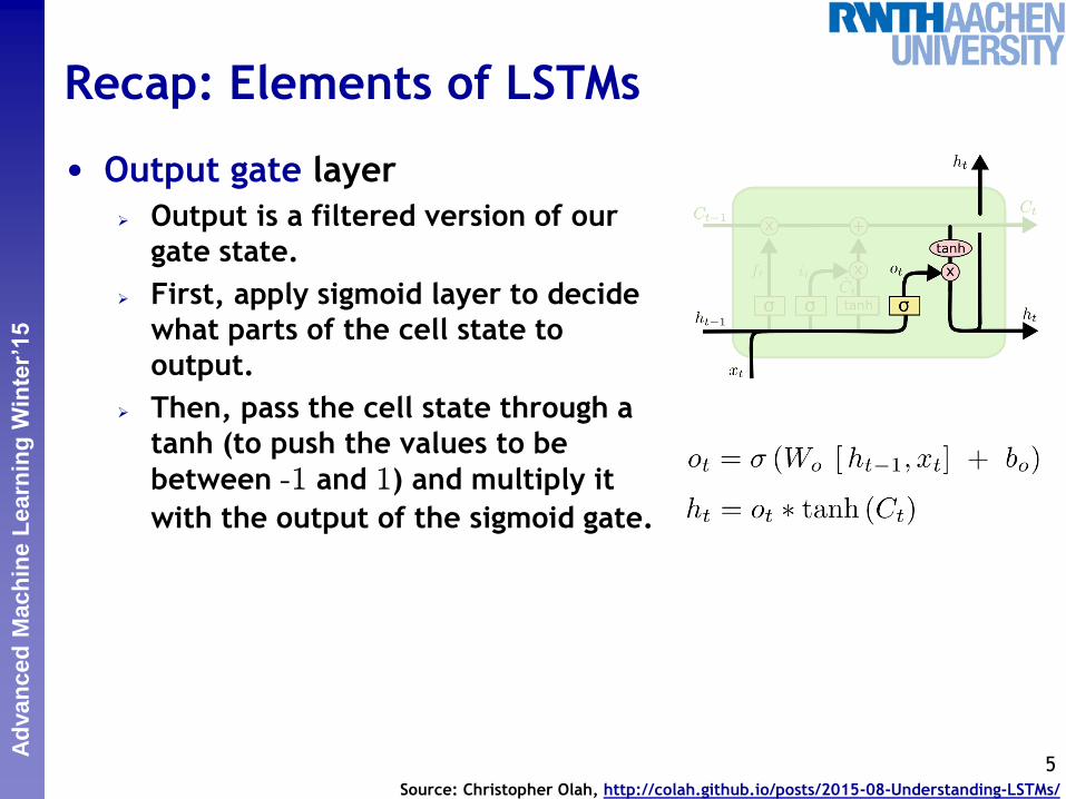
Recap: Elements of LSTMs
• Output gate layer
Output is a filtered version of our
gate state.
First, apply sigmoid layer to decide
what parts of the cell state to
output.
Then, pass the cell state through a
tanh (to push the values to be
between -1 and 1) and multiply it
with the output of the sigmoid gate.
5 Source: Christopher Olah, http://colah.github.io/posts/2015-08-Understanding-LSTMs/
Perc
eptu
al
and S
enso
ry A
ugm
ente
d C
om
puti
ng
Ad
van
ced
Mach
ine L
earn
ing
Winter’15
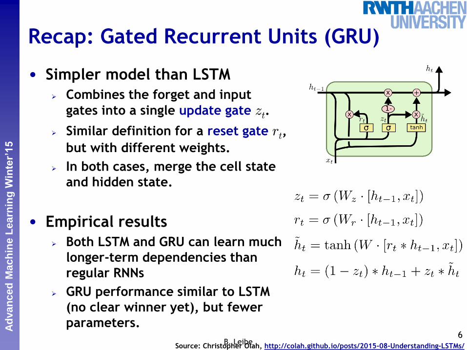
Recap: Gated Recurrent Units (GRU)
• Simpler model than LSTM
Combines the forget and input
gates into a single update gate zt.
Similar definition for a reset gate rt,
but with different weights.
In both cases, merge the cell state
and hidden state.
• Empirical results
Both LSTM and GRU can learn much
longer-term dependencies than
regular RNNs
GRU performance similar to LSTM
(no clear winner yet), but fewer
parameters. 6
B. Leibe Source: Christopher Olah, http://colah.github.io/posts/2015-08-Understanding-LSTMs/
Perc
eptu
al
and S
enso
ry A
ugm
ente
d C
om
puti
ng
Ad
van
ced
Mach
ine L
earn
ing
Winter’15
Topics of This Lecture
• Unsupervised Learning Motivation
• Energy based Models Definition
EBMs with Hidden Units
Learning EBMs
• Restricted Boltzmann Machines Definition
RBMs with Binary Units
RBM Learning
Contrastive Divergence
7 B. Leibe
Perc
eptu
al
and S
enso
ry A
ugm
ente
d C
om
puti
ng
Ad
van
ced
Mach
ine L
earn
ing
Winter’15
Looking Back...
• We have seen very powerful deep learning methods.
Deep MLPs
CNNs
RNNs (+LSTM, GRU)
(When used properly) they work very well and have achieved
great successes in the last few years.
• But...
All of those models have many parameters.
They need A LOT of training data to work well.
Labeled training data is very expensive.
How can we reduce the need for labeled data?
8 B. Leibe

Perc
eptu
al
and S
enso
ry A
ugm
ente
d C
om
puti
ng
Ad
van
ced
Mach
ine L
earn
ing
Winter’15
Reducing the Need for Labeled Data
• Reducing Model Complexity
E.g., GoogLeNet: big reduction in the number of parameters
compared to AlexNet (60M 5M).
More efficient use of the available training data.
• Transfer Learning
Idea: Pre-train a model on a large data corpus (e.g., ILSVRC),
then just fine-tune it on the available task data.
This is what is currently done in Computer Vision.
Benefit from generic representation properties of the pre-
trained model.
• Unsupervised / Semi-supervised Learning
Idea: Try to learn a generic representation from unlabeled data
and then just adapt it for the supervised classification task.
9 B. Leibe
Perc
eptu
al
and S
enso
ry A
ugm
ente
d C
om
puti
ng
Ad
van
ced
Mach
ine L
earn
ing
Winter’15
Topics of This Lecture
• Unsupervised Learning Motivation
• Energy based Models Definition
EBMs with Hidden Units
Learning EBMs
• Restricted Boltzmann Machines Definition
RBMs with Binary Units
RBM Learning
Contrastive Divergence
10 B. Leibe
Perc
eptu
al
and S
enso
ry A
ugm
ente
d C
om
puti
ng
Ad
van
ced
Mach
ine L
earn
ing
Winter’15
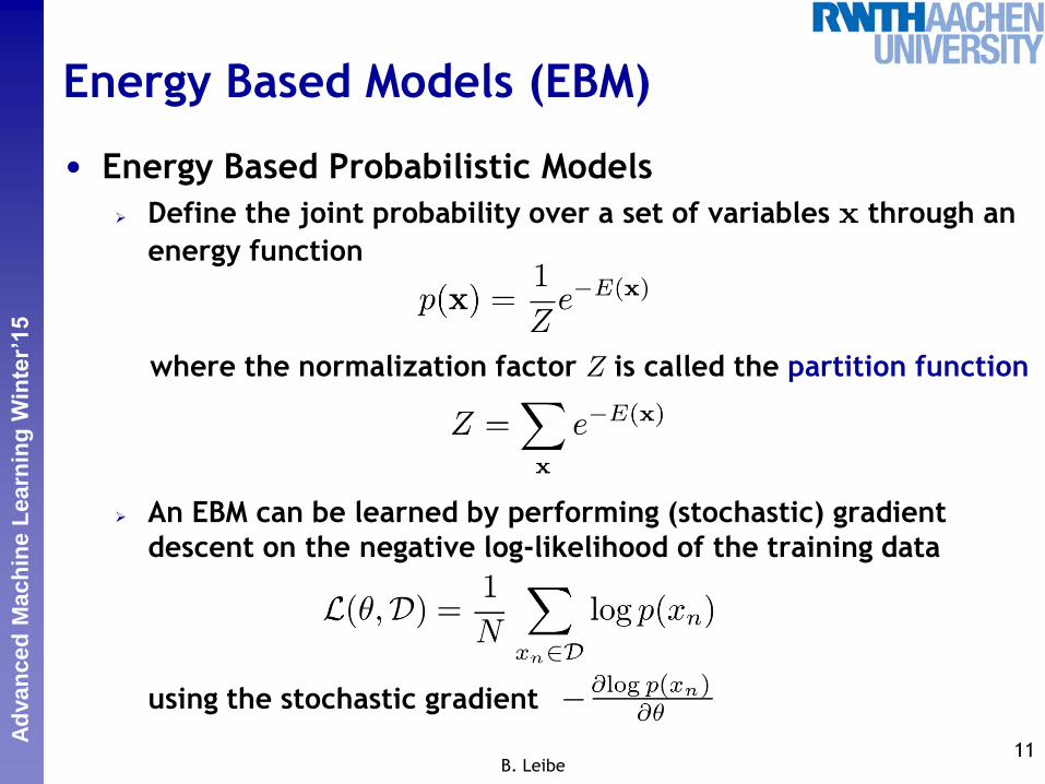
Energy Based Models (EBM)
• Energy Based Probabilistic Models
Define the joint probability over a set of variables x through an
energy function
where the normalization factor Z is called the partition function
An EBM can be learned by performing (stochastic) gradient
descent on the negative log-likelihood of the training data
using the stochastic gradient
11 B. Leibe
Perc
eptu
al
and S
enso
ry A
ugm
ente
d C
om
puti
ng
Ad
van
ced
Mach
ine L
earn
ing
Winter’15
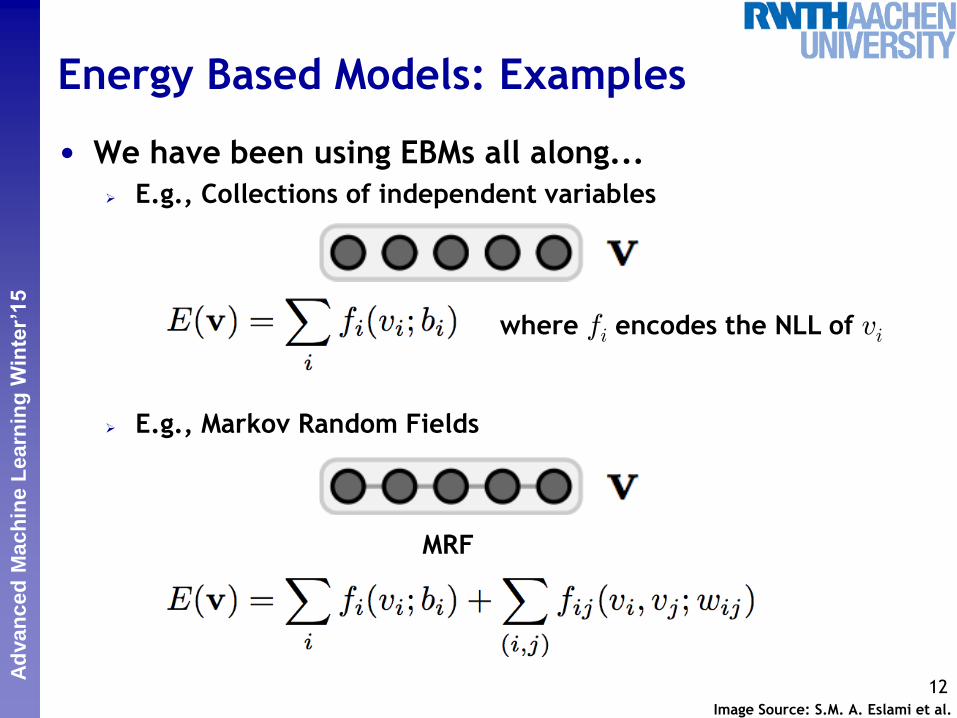
Energy Based Models: Examples
• We have been using EBMs all along...
E.g., Collections of independent variables
E.g., Markov Random Fields
12 Image Source: S.M. A. Eslami et al.
MRF
where fi encodes the NLL of vi
Perc
eptu
al
and S
enso
ry A
ugm
ente
d C
om
puti
ng
Ad
van
ced
Mach
ine L
earn
ing
Winter’15
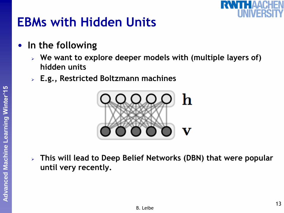
• In the following
We want to explore deeper models with (multiple layers of)
hidden units
E.g., Restricted Boltzmann machines
This will lead to Deep Belief Networks (DBN) that were popular
until very recently.
EBMs with Hidden Units
13 B. Leibe
Perc
eptu
al
and S
enso
ry A
ugm
ente
d C
om
puti
ng
Ad
van
ced
Mach
ine L
earn
ing
Winter’15
EBMs with Hidden Units
14 B. Leibe
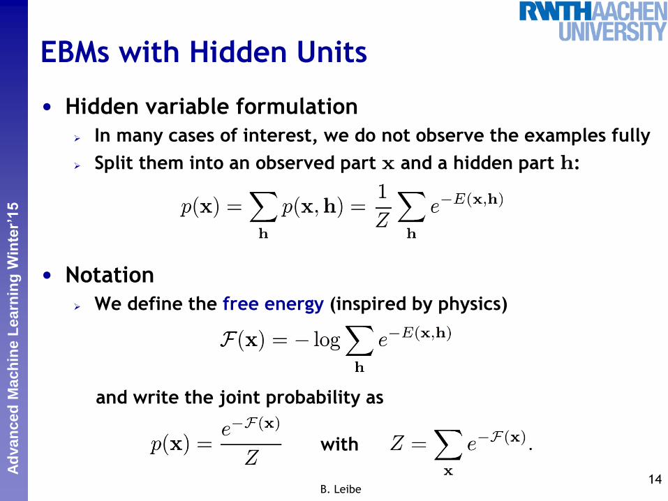
• Hidden variable formulation
In many cases of interest, we do not observe the examples fully
Split them into an observed part x and a hidden part h:
• Notation
We define the free energy (inspired by physics)
and write the joint probability as
with
Perc
eptu
al
and S
enso
ry A
ugm
ente
d C
om
puti
ng
Ad
van
ced
Mach
ine L
earn
ing
Winter’15
EBMs with Hidden Units
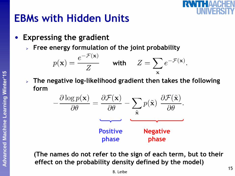
• Expressing the gradient
Free energy formulation of the joint probability
The negative log-likelihood gradient then takes the following
form
(The names do not refer to the sign of each term, but to their
effect on the probability density defined by the model) 15
B. Leibe
with
Positive
phase
Negative
phase

Perc
eptu
al
and S
enso
ry A
ugm
ente
d C
om
puti
ng
Ad
van
ced
Mach
ine L
earn
ing
Winter’15
Challenge for Learning
16 B. Leibe
• Problem
Difficult to determine this gradient analytically.
Computing it would involve evaluating
i.e., the expectation over all possible configurations of the input
x under the distribution p formed by the model!
Often infeasible.
Ep
·@F(x)
@µ
¸
Perc
eptu
al
and S
enso
ry A
ugm
ente
d C
om
puti
ng
Ad
van
ced
Mach
ine L
earn
ing
Winter’15
Steps Towards a Solution...
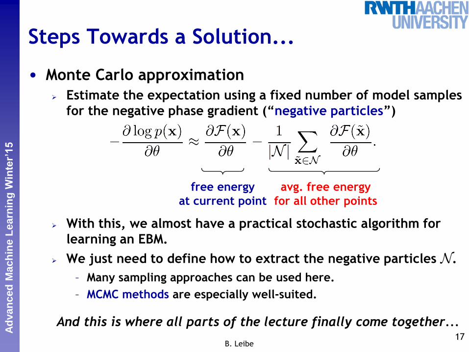
• Monte Carlo approximation
Estimate the expectation using a fixed number of model samples
for the negative phase gradient (“negative particles”)
With this, we almost have a practical stochastic algorithm for
learning an EBM.
We just need to define how to extract the negative particles N.
– Many sampling approaches can be used here.
– MCMC methods are especially well-suited.
And this is where all parts of the lecture finally come together... 17
B. Leibe
free energy
at current point
avg. free energy
for all other points
Perc
eptu
al
and S
enso
ry A
ugm
ente
d C
om
puti
ng
Ad
van
ced
Mach
ine L
earn
ing
Winter’15
Topics of This Lecture
• Unsupervised Learning Motivation
• Energy based Models Definition
EBMs with Hidden Units
Learning EBMs
• Restricted Boltzmann Machines Definition
RBMs with Binary Units
RBM Learning
Contrastive Divergence
18 B. Leibe
Perc
eptu
al
and S
enso
ry A
ugm
ente
d C
om
puti
ng
Ad
van
ced
Mach
ine L
earn
ing
Winter’15
Restricted Boltzmann Machines (RBM)
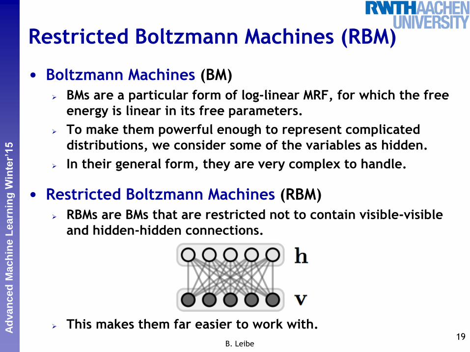
• Boltzmann Machines (BM)
BMs are a particular form of log-linear MRF, for which the free
energy is linear in its free parameters.
To make them powerful enough to represent complicated
distributions, we consider some of the variables as hidden.
In their general form, they are very complex to handle.
• Restricted Boltzmann Machines (RBM)
RBMs are BMs that are restricted not to contain visible-visible
and hidden-hidden connections.
This makes them far easier to work with.
19
B. Leibe
Perc
eptu
al
and S
enso
ry A
ugm
ente
d C
om
puti
ng
Ad
van
ced
Mach
ine L
earn
ing
Winter’15
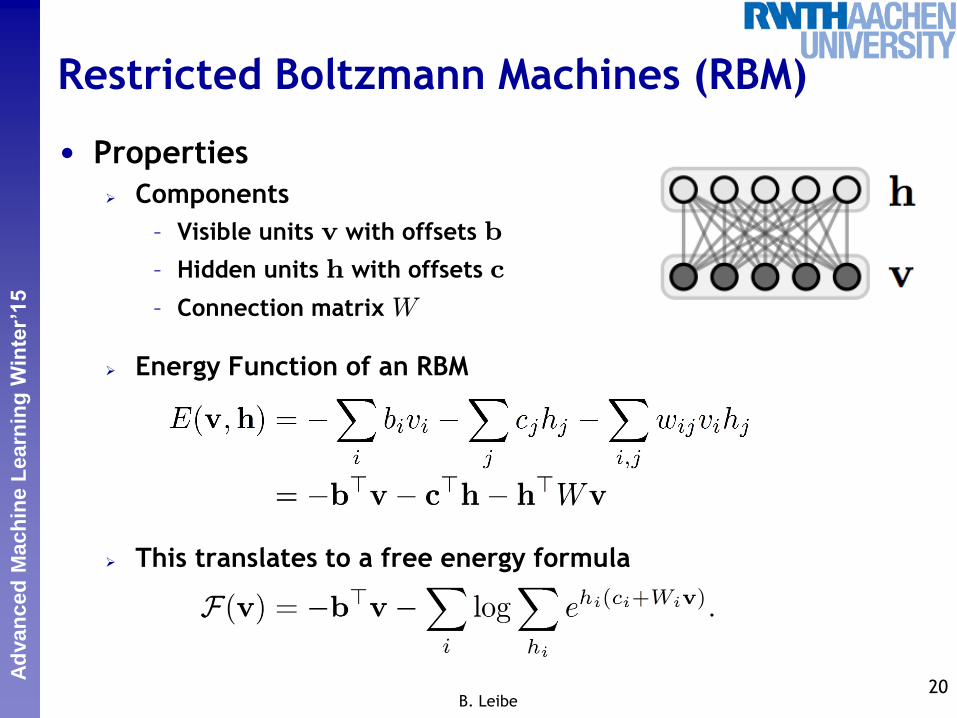
• Properties
Components
– Visible units v with offsets b
– Hidden units h with offsets c
– Connection matrix W
Energy Function of an RBM
This translates to a free energy formula
Restricted Boltzmann Machines (RBM)
20 B. Leibe
Perc
eptu
al
and S
enso
ry A
ugm
ente
d C
om
puti
ng
Ad
van
ced
Mach
ine L
earn
ing
Winter’15
Restricted Boltzmann Machines (RBM)
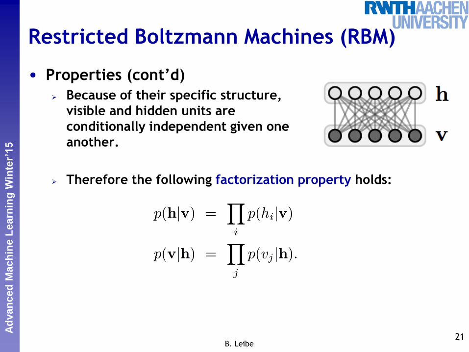
• Properties (cont’d)
Because of their specific structure,
visible and hidden units are
conditionally independent given one
another.
Therefore the following factorization property holds:
21 B. Leibe

Perc
eptu
al
and S
enso
ry A
ugm
ente
d C
om
puti
ng
Ad
van
ced
Mach
ine L
earn
ing
Winter’15
Restricted Boltzmann Machines (RBM)
• Interpretation of RBMs
Factorization property
RBMs can be seen as a product of experts specializing on
different areas.
Experts detect negative constraints, if one of them returns
zero, the entire product is zero.
22 B. Leibe
Perc
eptu
al
and S
enso
ry A
ugm
ente
d C
om
puti
ng
Ad
van
ced
Mach
ine L
earn
ing
Winter’15
RBMs with Binary Units
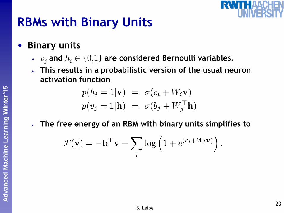
• Binary units
vj and hi 2 {0,1} are considered Bernoulli variables.
This results in a probabilistic version of the usual neuron
activation function
The free energy of an RBM with binary units simplifies to
23 B. Leibe
Perc
eptu
al
and S
enso
ry A
ugm
ente
d C
om
puti
ng
Ad
van
ced
Mach
ine L
earn
ing
Winter’15
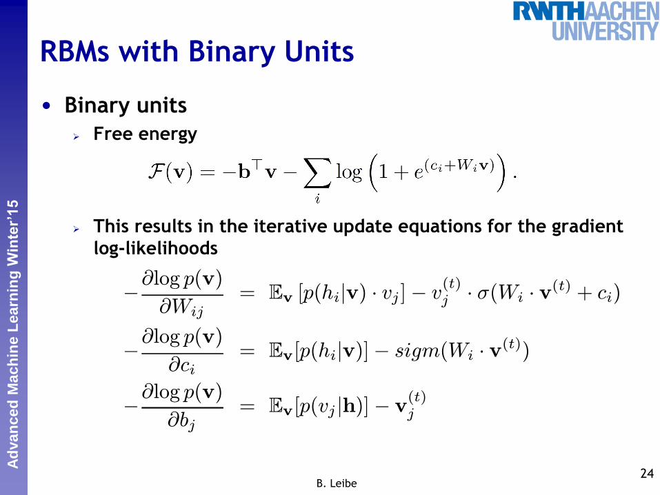
RBMs with Binary Units
• Binary units
Free energy
This results in the iterative update equations for the gradient
log-likelihoods
24
B. Leibe
¡@log p(v)
@Wij
= Ev [p(hijv) ¢ vj ]¡ v(t)
j ¢ ¾(Wi ¢ v(t) + ci)
¡@log p(v)
@ci= Ev[p(hijv)]¡ sigm(Wi ¢ v(t))
¡@log p(v)
@bj= Ev[p(vj jh)]¡ v
(t)
j
Perc
eptu
al
and S
enso
ry A
ugm
ente
d C
om
puti
ng
Ad
van
ced
Mach
ine L
earn
ing
Winter’15
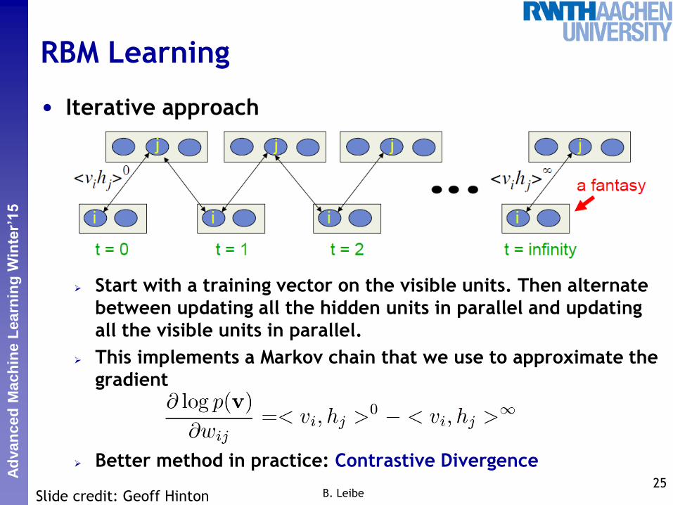
RBM Learning
• Iterative approach
Start with a training vector on the visible units. Then alternate
between updating all the hidden units in parallel and updating
all the visible units in parallel.
This implements a Markov chain that we use to approximate the
gradient
Better method in practice: Contrastive Divergence 25
B. Leibe Slide credit: Geoff Hinton
Perc
eptu
al
and S
enso
ry A
ugm
ente
d C
om
puti
ng
Ad
van
ced
Mach
ine L
earn
ing
Winter’15
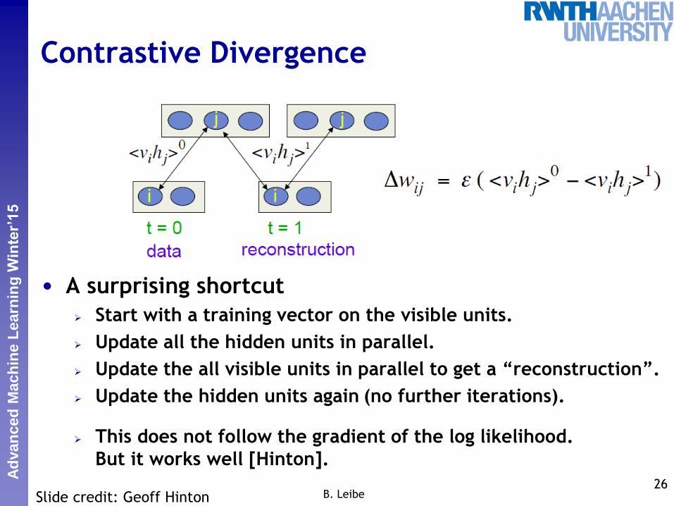
Contrastive Divergence
• A surprising shortcut
Start with a training vector on the visible units.
Update all the hidden units in parallel.
Update the all visible units in parallel to get a “reconstruction”.
Update the hidden units again (no further iterations).
This does not follow the gradient of the log likelihood.
But it works well [Hinton].
26 B. Leibe Slide credit: Geoff Hinton
Perc
eptu
al
and S
enso
ry A
ugm
ente
d C
om
puti
ng
Ad
van
ced
Mach
ine L
earn
ing
Winter’15
Example
• RBM training on MNIST
Persistent Contrastive Divergence with chain length 15 27
B. Leibe
Perc
eptu
al
and S
enso
ry A
ugm
ente
d C
om
puti
ng
Ad
van
ced
Mach
ine L
earn
ing
Winter’15
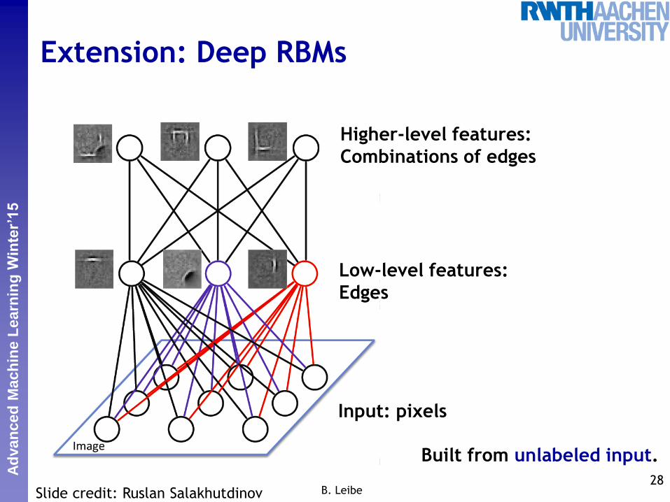
Extension: Deep RBMs
28 B. Leibe
Input: pixels
Low-level features:
Edges
Higher-level features:
Combinations of edges
Built from unlabeled input.
Slide credit: Ruslan Salakhutdinov