Advanced Machine Learning Techniques for Temporal,

Multimedia, and Relational Data

Vibhav Gogate

The University of Texas at Dallas

1 Vibhav Gogate

Many slides courtesy of Kevin Murphy

Multimedia Data • Text

o Ascii documents o HTML documents o Databases (Structured documents) o Annotations

• Images o JPG, PNG, BMP, TIFF, etc.

• Audio o MP3, WAV files

• Video o Sequence of frames

Size and Complexity of processing the data increases as we go from top to bottom

2 Vibhav Gogate

Temporal Data

• Time Series data generated by a dynamic system

o A user’s GPS locations recorded by his Cell-phone

o Loop Sensors counting cars on a freeway

o Load monitoring devices capturing power consumed in a household

o Video as a sequence of frames

Vibhav Gogate 3

Relational Data

• Data resides in multiple tables

Vibhav Gogate 4

Example Borrowed from Luc De Raedt’s textbook, “Logical and Relational Learning”

Machine Learning

• Study of systems that improve their performance over time with experience

• Experience= Data (or examples or observations or evidence)

• Learning = Search for patterns, regularities or rules that provide insights into the data

Vibhav Gogate 5

What we will cover?

• Probabilistic Machine Learning

o Build a model that describes the distribution that generated the data

o Representation, Inference and Learning

• Dynamic Probabilistic Networks

o Temporal Data

• Markov Logic Networks

o Relational Data

Vibhav Gogate 6

Probabilistic Graphical Models • “PGMs have revolutionized AI and machine

learning over the last two decades” – Eric Horvitz, Director, Microsoft Research

• Basic Idea: Compactly represent a joint probability distribution over a large number of variables by taking advantage of conditional independence. o Graph describes the conditional independence

assumptions

Vibhav Gogate 7

Bayesian networks

• Directed or Causal Networks

Vibhav Gogate 8

Product of several poly-sized conditional probability tables

Each table is variable given its parents in the graph

Bayesian networks

Vibhav Gogate 9

Joint distribution

…………………………………….. ……………………………………..

0.2 × 0.05 × .6 × .8 × .3 = .00144

31 vs 17 entries Exponential vs Poly entries

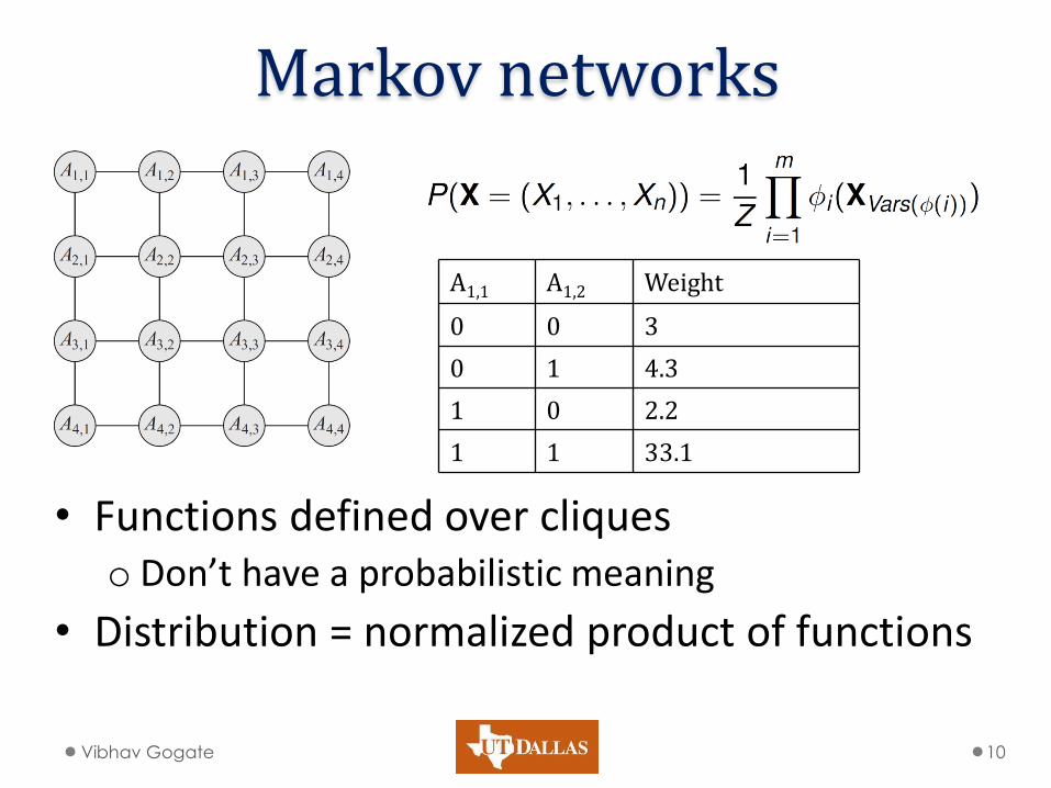
Markov networks

• Functions defined over cliques o Don’t have a probabilistic meaning

• Distribution = normalized product of functions

Vibhav Gogate 10

A1,1 A1,2 Weight

0 0 3

0 1 4.3

1 0 2.2

1 1 33.1

Log-Linear models

• PGM = A set of weighted formulas (features) in propositional logic

• Alternative Representation of a PGM

• Distribution

Vibhav Gogate 11

Inference Problems • Probability of Evidence (PR)

o Find the probability of an assignment to a subset of variables

• Conditional Marginal Estimation (MAR) o Find the marginal probability distribution at a variable

given evidence

• Maximum a Posteriori (MAP) o Find an assignment with the maximum probability given

evidence

• All of them are at least NP-hard

Vibhav Gogate 12

Learning problems

• Structure Learning

o Learn the structure of the graph from data

• Weight Learning

o Learn the parameters (CPTs, weights of features)

• Structure Learning is often much harder than weight learning

• In practice, we often assume a structure

Vibhav Gogate 13

Inference algorithms

• Exact algorithms

o Exponential in treewidth (a graph parameter)

• Message-passing algorithms

o Belief propagation, Expectation propagation, etc.

• Sampling algorithms

o Importance sampling

oMarkov chain Monte Carlo sampling

• Gibbs sampling

Vibhav Gogate 14

Dynamic Bayesian networks

• PGMs are static; don’t have a concept of time

• Dynamic Bayesian networks are temporal PGMs

• Three assumptions

o Stationary

o Time is discrete

o K-Markov assumption

Vibhav Gogate 15

Dynamic Bayesian networks

Vibhav Gogate 16

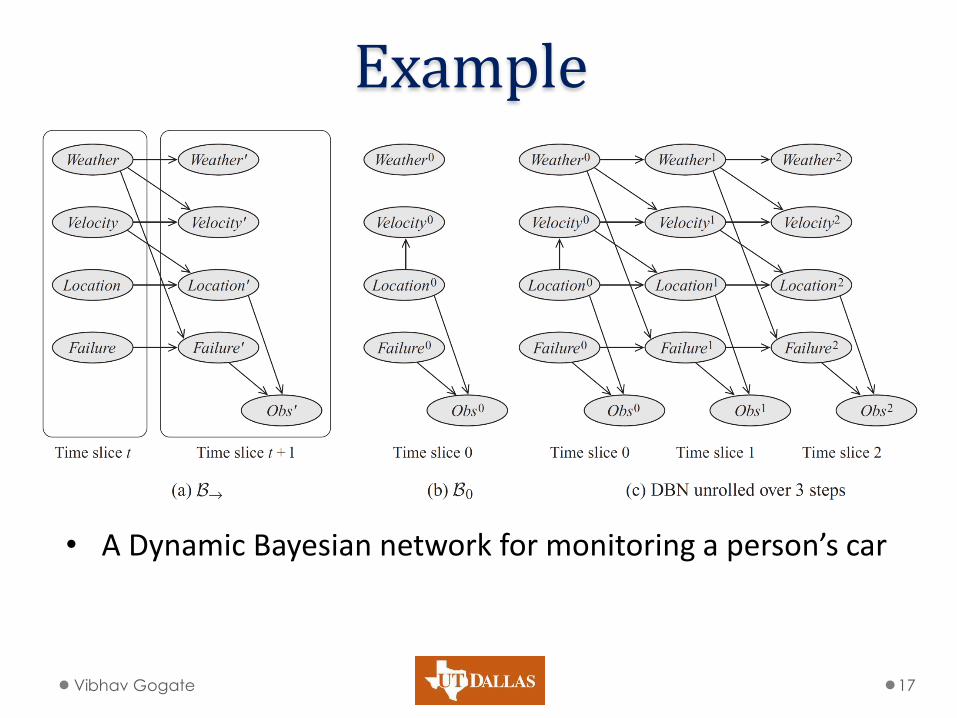
Example

• A Dynamic Bayesian network for monitoring a person’s car

Vibhav Gogate 17

A DBN as a HMM

• Hidden Markov models (HMMs)

o Each time slice has one cluster each for observed and unobserved variables

Vibhav Gogate 18

Vibhav Gogate 19

Factorial HMMs as DBNs

• Example: Several sources of sound from a single microphone

Vibhav Gogate 20

Factorial HMM

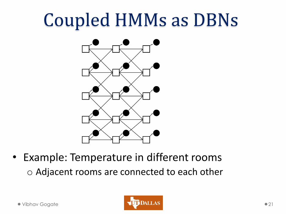
Coupled HMMs as DBNs

• Example: Temperature in different rooms o Adjacent rooms are connected to each other

Vibhav Gogate 21

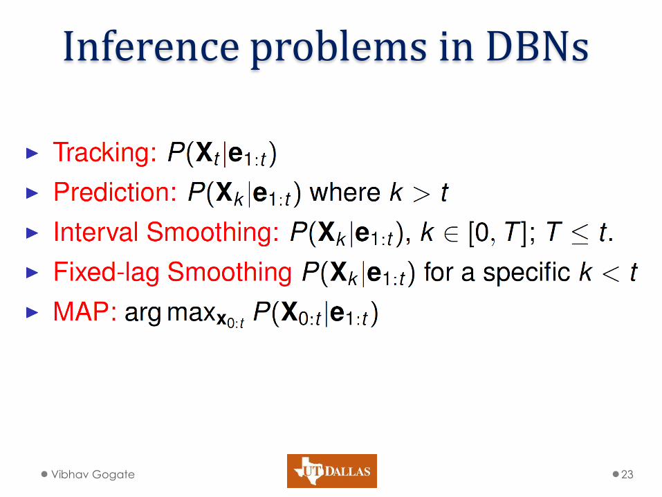
Inference problems in DBNs • Tracking or Filtering

o Find the probability distribution over all variables or the marginal distribution at a variable at time slice “t” given evidence up to slice “t”

• Prediction o Find the probability distribution at time slice “k” given

evidence up to slice “t” where k>t.

• Smoothing o Find the probability distribution at time slice “k” given

evidence up to slice “t” where k<t.

• MAP inference o Find the most likely trajectory of the system.

Vibhav Gogate 22

Inference problems in DBNs

Vibhav Gogate 23

Application Designer

• Select the variables at each time-slice

• Select the edges by following sound probabilistic principles

o The networks should be a directed acyclic graph (DAG)

o Each variable should be independent of its non-descendants given its parents

o Sparesity: Limit the number of parents at each variable

Vibhav Gogate 24

Application Designer

• Remember as you increase the number of variables:

o The model looks realistic

o However, the complexity of inference and learning increases and the accuracy goes down because we have to use approximate inference methods

o Tradeoff between the two is rarely explored in practice

• Don’t think of the technology as a black-box

o We are not there yet!

Vibhav Gogate 25

Tracking/Filtering Algorithms

• Exact Inference

• Approximate Message passing algorithms

• Sampling Algorithms

o Particle Filtering

o Rao-Blackwellised Particle Filtering

Vibhav Gogate 26

Exact Inference on HMMs

Vibhav Gogate 27

Exact Inference in HMMs

• Procedural view o Cluster (X0) stores P(X0) o Each cluster (Xt,Xt+1) stores P(Xt+1|Xt) and P(Et+1|Xt+1)

• Multiply incoming message with the functions • Sum-out Xt and send the resulting function to the

next cluster

Vibhav Gogate 28

X0 X1 X2

E1 E2

X0X1 X1X2 X0

Unrolled HMM

Message-passing algorithm

Exact Inference in DBNs

• Clusters are Factored!

Vibhav Gogate 29

At

Ct

Bt

Dt

At+1

Ct+1

Bt+1

Dt+1

Et Et+1

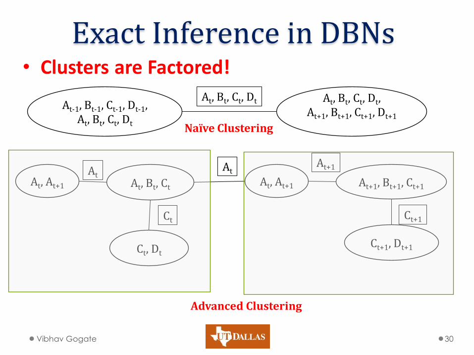
Exact Inference in DBNs • Clusters are Factored!

Vibhav Gogate 30

At, Bt, Ct, Dt, At+1, Bt+1, Ct+1, Dt+1

At-1, Bt-1, Ct-1, Dt-1, At, Bt, Ct, Dt

At, Bt, Ct, Dt

Naïve Clustering

At+1, Bt+1, Ct+1

Ct+1, Dt+1

Ct+1

At, Bt, Ct

Ct, Dt

At

Ct

Advanced Clustering

At, At+1 At, At+1 At

At+1

Smaller Clusters • Complexity: exponential in the number of variables

in the cluster o Smaller clusters are desirable

• How to construct the clusters? o At each time slice, find which nodes are connected to

the next time slice and create a clique over them • Interface nodes

o At each time slice, create a junction tree out of • Moralized graph over nodes in the time slice • Interface cliques over the time slice and previous one

o Paste the junction trees together.

Vibhav Gogate 31

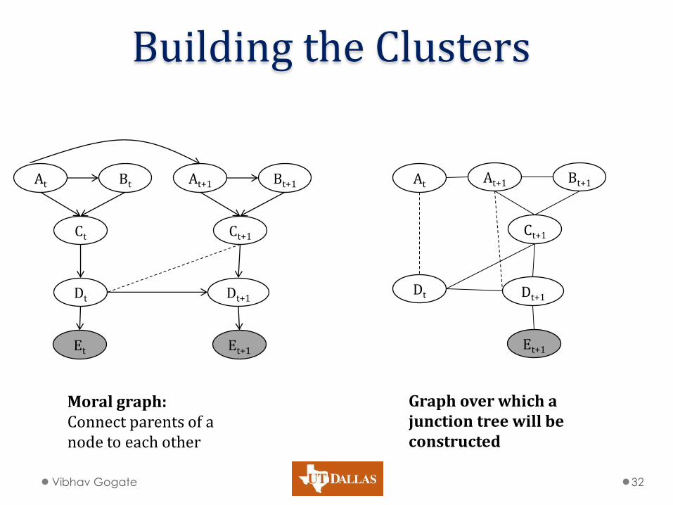
Building the Clusters

Vibhav Gogate 32

At

Ct

Bt

Dt

At+1

Ct+1

Bt+1

Dt+1

Et Et+1

Moral graph: Connect parents of a node to each other

At+1

Ct+1

Bt+1

Dt+1

Et+1

At

Dt

Graph over which a junction tree will be constructed

Building the Clusters

• Make Graph Chordal

• Process nodes in order o Create a clique out of all nodes

ordered below the node (its children) and having an edge with the node

E

D

F

B

C

A

A

B

C

D

E

F

Chordal Graph Junction Tree

E

D

F

B

C

A ABC

EFC

DBCF

FBC

BC

C

BC FC

FBC

BC

C

At each node: Construct a cluster out of the variable and its children

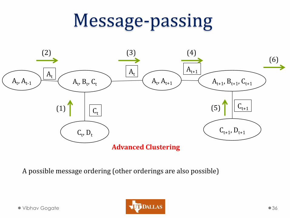
Message-passing • At each slice

o Put each function in a cluster that contains all variables mentioned in the function

o Order messages such that the outgoing interface message is the last one computed

o Perform message passing • Multiply all incoming messages with the functions in the

cluster

• Sum-out all variables that are mentioned in the cluster but not mentioned in the receiving cluster.

Vibhav Gogate 35

Message-passing

Vibhav Gogate 36

At+1, Bt+1, Ct+1

Ct+1, Dt+1

Ct+1

At, Bt, Ct

Ct, Dt

At

Ct

Advanced Clustering

At, At+1 At, At-1 At

At+1

(1)

(2) (3) (4)

(5)

(6)

A possible message ordering (other orderings are also possible)

Why it works? • Laws of probability theory

• It turns out that o P(Xt|X1:t-1,e1:t-1,et)=P(Xt|It-1,et)

o Namely, Xt is conditionally independent of the past given the interface nodes It-1at time slice t-1.

• The message passing algorithm is an instance of the variable elimination algorithm o Eliminate all variables except the ones required by

the next time slice

Vibhav Gogate 37

Approximate Inference

• Sometimes the cluster size is just too large to allow exact inference

• Resort to approximate inference

oMessage Passing

o Sampling-based

Vibhav Gogate 38

Approximate Message Passing

Vibhav Gogate 39

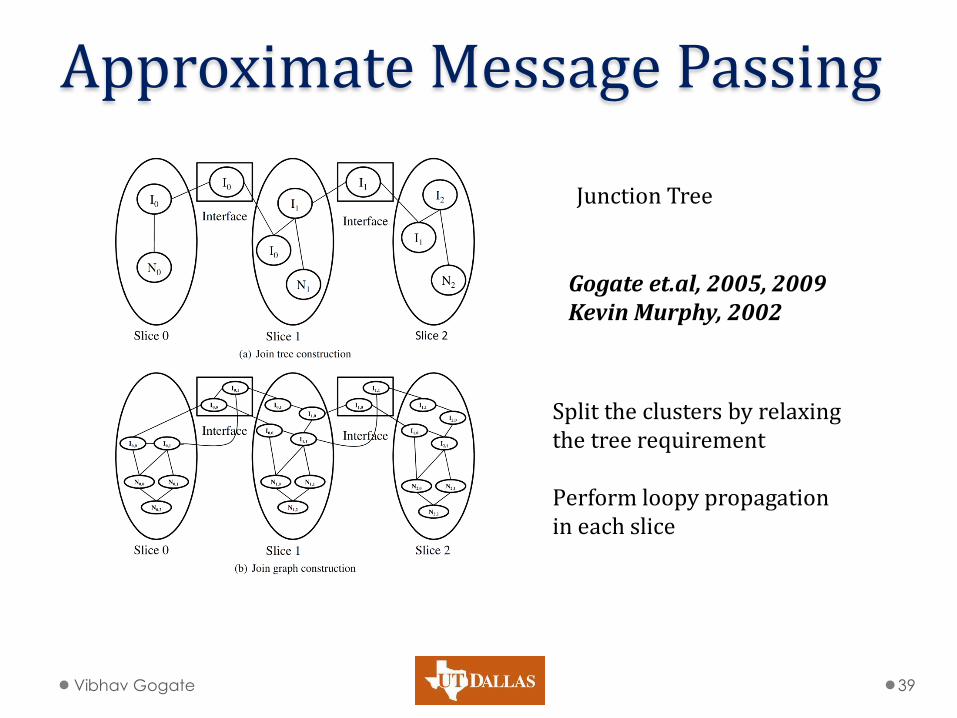
Junction Tree

Split the clusters by relaxing the tree requirement Perform loopy propagation in each slice

Gogate et.al, 2005, 2009 Kevin Murphy, 2002

Iterative Join Graph Propagation

G

E

F

C D

B

A

a) schematic mini-bucket(i), i=3 b) arc-labeled join-graph decomposition

CDB

CAB

BA

A

CB P(D|B)

P(C|A,B)

P(A)

BA

P(B|A)

FCD

P(F|C,D)

GFE

EBF

BF

EF P(E|B,F)

P(G|F,E)

B

CD

BF

A

F

G: (GFE)

E: (EBF) (EF)

F: (FCD) (BF)

D: (DB) (CD)

C: (CAB) (CB)

B: (BA) (AB) (B)

A: (A)

Message passing Equations

• Multiply all received messages except from R

• Multiply all functions

• Sum-out all variables except the separator

S

R

𝑚 𝑆 → 𝑅 = 𝑓 𝑚(

𝐺∈𝑁𝑒𝑖𝑔𝑕𝑏𝑜𝑟𝑠 𝑆 −𝑅𝑓∈𝑓𝑢𝑛𝑐𝑡𝑖𝑜𝑛𝑠(𝑆)𝑉𝑎𝑟𝑠 𝑆 −𝑆𝑒𝑝(𝑆,𝑅)

G → R)

Particle Filtering

• At each time slice

o Generate N particles from a distribution Q

• It is difficult to sample from P

o Compute the weight of each particle

• Correct for the fact that you are sampling from Q and not the target distribution P

o Represent the belief state using the weighted particles

Vibhav Gogate 42

Particle Filtering

Vibhav Gogate 43

Particle Filtering: Picture

Vibhav Gogate 44

Impact of the Resampling Step

Vibhav Gogate 45

Rao-Blackwellised Particle Filtering

Vibhav Gogate 46

Rao-Blackwellised Particle Filtering

Vibhav Gogate 47

At+1, Bt+1, Ct+1

Ct+1, Dt+1

Ct+1

At, Bt, Ct

Ct, Dt

At

Ct

At, At+1 At, At-1 At

At+1

(1)

(2) (3) (4)

(5)

(6)

• Suppose we have enough computational resources to do inference with two variables in each cluster!

• Sample Bt at each time slice, Exactly infer others!

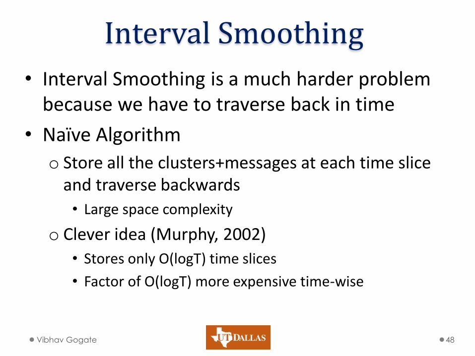
Interval Smoothing

• Interval Smoothing is a much harder problem because we have to traverse back in time

• Naïve Algorithm

o Store all the clusters+messages at each time slice and traverse backwards

• Large space complexity

o Clever idea (Murphy, 2002)

• Stores only O(logT) time slices

• Factor of O(logT) more expensive time-wise

Vibhav Gogate 48

MAP estimation

• Instead of using sum-out operation we use a max-out operation.

Vibhav Gogate 49

Parameter Learning: FOD

• FOD: fully observable data

Vibhav Gogate 50

Parameter Learning: POD

• POD: Partially observable data

Vibhav Gogate 51

Handling Continuous variables

• Dependencies are often modeled as linear Gaussian

• Example: Current position (X) and Velocity (V)

o P(Xt|Xt-1,Vt)=Xt-1+Vt+N(0;2X); : length of slice

o P(Vt|Vt-1)=Vt-1+N(0;2V)

• Conditional linear Gaussian

o Continuous variables have discrete parents

• Hybrid Particle Filtering and GBP algorithms

Vibhav Gogate 52

Applications

• Recognizing activities and transportation routines

• Robotics

• Object tracking

• Bio-informatics

• Speech recognition

• Event detection in Videos

Vibhav Gogate 53

Recognizing travel routines D: Time-of-day (discrete)

W: Day of week (discrete)

Goal: collection of locations where the

person spends significant amount of

time. (discrete)

Route: A hidden variable that just

predicts what path the person takes

(discrete)

Location: A pair (e,d) e is the edge on

which the person is and d is the

distance of the person from one of the

end-points of the edge (continuous)

Velocity: Continuous

GPS reading: (lat,lon,spd,utc).

yt

gt-1

rt-1

lt-1

yt-1

vt-1

gt

rt

lt

vt

dt-1 wt-1

dt wt

Example Queries

• Where the person will be 10 minutes from now?

o P(lT|d1:t,w1:t,y1:t) where T=t+10 minutes

• What is the person’s next goal?

o P(gT|d1:t,w1:t,y1:t)

Example of Goals

Example of Route

Route Seen

Route Predicted

Grocery

store

Experimental Results: Data Collection

• GPS data was collected by one of the authors for a period of 6 months. o Latitude and longitude pairs

• 3 months data was used for training and 3 months for testing.

• Data divided into segments o A segment is a series of GPS readings such that two

consecutive readings are less than 15 minutes apart.

Experimental Results: Models and algorithms

• Test if adding new variables improves prediction accuracy. o Model-1: Model as described before

o Model-2: Remove variables dt and wt

o Model-3: Remove variables dt, wt,ft,rt,gt from each time slice.

• Algorithms: o IJGP-RBPF(1,2), IJGP-RBPF(2,1), IJGP-S(1) and IJGP-S(2)

Learning the models from data • EM algorithm used for learning the models

• Takes about 3 to 5 days to learn data that is distributed over 3 months.

• Since EM uses inference as a sub-step, we have 4 EM algorithms corresponding to the 4 algorithms used for inference

o IJGP-RBPF(1,2), IJGP-RBPF(2,1), IJGP-S(1) and IJGP-S(2)

Predicting Goals (MODEL-1)

• Compute P(gt|e1:t) and compare it with the actual goal.

• Accuracy = percentage of goals predicted correctly.

• N = number of particles

• Column: learning algorithm

• Row: inference algorithm

Model-1 (20% of the trip seen)

N Inference\Learning IJGP-RBPF(1,1) IJGP-RBPF(1,2) IJGP(1) IJGP(2)

Time Accuracy Accuracy Accuracy Accuracy

100 IJGP-RBPF(1,1) 12.3 78 80 79 80

100 IJGP-RBPF(1,2) 15.8 81 84 78 81

200 IJGP-RBPF(1,1) 33.2 80 84 77 82

200 IJGP-RBPF(1,2) 60.3 80 84 76 82

500 IJGP-RBPF(1,1) 123.4 81 84 80 82

500 IJGP-RBPF(1,2) 200.12 84 84 81 82

IJGP(1) 9 79 79 77 79

IJGP(2) 34.3 74 84 78 82

Predicting Goals (Model-2)

IJGP-RBPF(1,1) IJGP-RBPF(1,2) IJGP(1) IJGP(2)

N Inference\Learning Time Accuracy Accuracy Accuracy Accuracy

100 IJGP-RBPF(1,1) 8.3 73 73 71 73

100 IJGP-RBPF(1,2) 14.5 76 76 71 75

200 IJGP-RBPF(1,1) 23.4 76 77 71 75

200 IJGP-RBPF(1,2) 31.4 76 77 71 76

500 IJGP-RBPF(1,1) 40.08 76 77 71 76

500 IJGP-RBPF(1,2) 51.87 76 77 71 76

IJGP(1) 6.34 71 73 71 74

IJGP(2) 10.78 76 76 72 76

•Compute P(gt|e1:t) and compare it with the actual goal. •Accuracy = percentage of goals predicted correctly. •N = number of particles •Column: learning algorithm •Row: inference algorithm

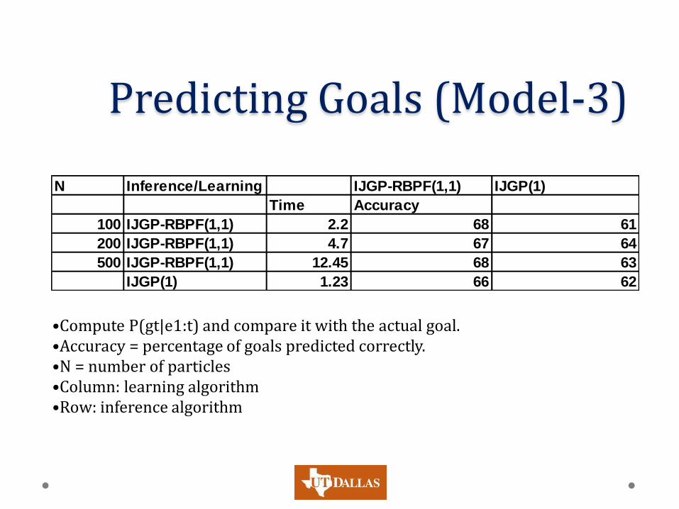
Predicting Goals (Model-3)

N Inference/Learning IJGP-RBPF(1,1) IJGP(1)

Time Accuracy

100 IJGP-RBPF(1,1) 2.2 68 61

200 IJGP-RBPF(1,1) 4.7 67 64

500 IJGP-RBPF(1,1) 12.45 68 63

IJGP(1) 1.23 66 62

•Compute P(gt|e1:t) and compare it with the actual goal. •Accuracy = percentage of goals predicted correctly. •N = number of particles •Column: learning algorithm •Row: inference algorithm

Predicting Routes • Compare the path of the person predicted by the

model with the actual path.

• False positives (FP)

o count the number of roads that were not taken by the person but were in the predicted path.

• False Negatives (FN)

o count the number of roads that were taken by the person but were not in the predicted path.

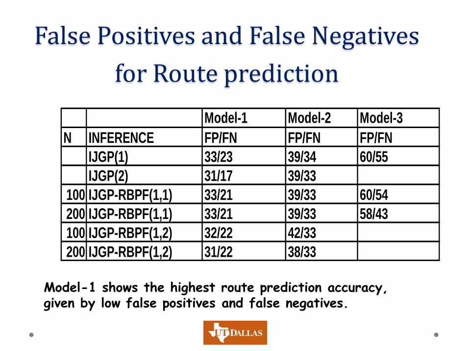
False Positives and False Negatives

for Route prediction

Model-1 Model-2 Model-3

N INFERENCE FP/FN FP/FN FP/FN

IJGP(1) 33/23 39/34 60/55

IJGP(2) 31/17 39/33

100 IJGP-RBPF(1,1) 33/21 39/33 60/54

200 IJGP-RBPF(1,1) 33/21 39/33 58/43

100 IJGP-RBPF(1,2) 32/22 42/33

200 IJGP-RBPF(1,2) 31/22 38/33

Model-1 shows the highest route prediction accuracy, given by low false positives and false negatives.

Software

• BNT toolkit by Kevin Murphy

• GMTK toolkit by Jeff Bilmes

Vibhav Gogate 66