advanced manufacturing processes prof. apurbba …textofvideo.nptel.ac.in/112107078/lec29.pdf ·...
TRANSCRIPT

Advanced Manufacturing Processes
Prof. Apurbba Kumar Sharma
Department of Mechanical and Industrial Engineering
Indian Institute of Technology, Roorkee
Module - 3
Advanced Machining Processes
Lecture - 18
Electron Beam, Plasma Beam and Ion Beam Machining
Welcome to this session on design of tools in electrochemical machining under the
course advanced manufacturing processes. In the previous sessions on electrochemical
machining we have seen the principles, its applications, the components in ECM process
and so on. In this session let us discuss few things on design of tools on used for
electrochemical machining process. Generally, designing of a tool means determining
the shape of a tool. Why shape is important in electrochemical machining tool is that the
tool creates a replica on the work surface that means in turn the object to be prepared or
the profile to be machined on a work surface, work free surface should be replicated on
the tool which will in turn while put in action will produce the same replica on the work
free surface.
Therefore, once we know the profile to be produced the work profile or the surface to be
produced say a particular surface can be expressed in terms of some mathematical
equation, then what will be the corresponding surface or the profile of the tool to be used
for particular machine. So, this this is an important aspect in electrochemical machining
and little bit of mathematics is involved in this. So, we will try to derive out or the see
the mechanism how this can be arrived at the derivations and the final tool equation with
the help of some mathematical formulations.
(Refer Slide Time: 03:04)
Before moving into the derivation of the tool, let us briefly refresh our self with the
principles of working of ECM, kinematics and dynamics of ECM. The basic principles
that go on the ECM are the Faraday’s laws as we know. These laws are described like
this.
(Refer Slide Time: 03:35)
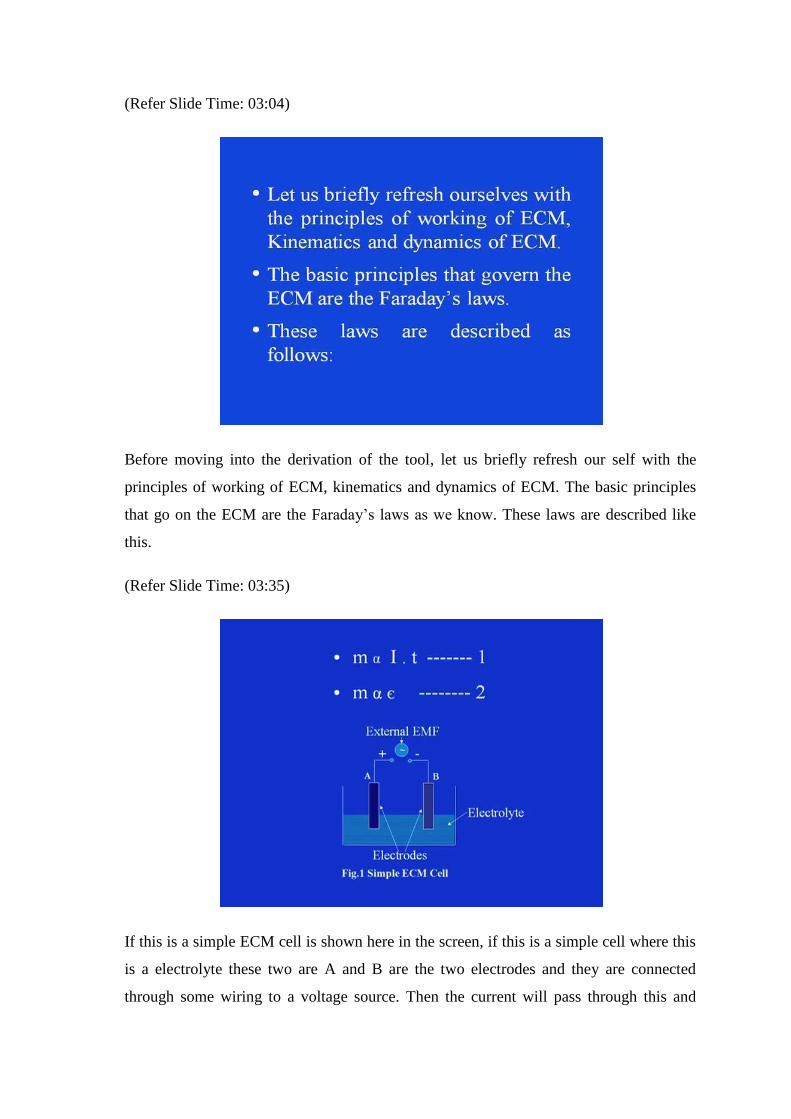
If this is a simple ECM cell is shown here in the screen, if this is a simple cell where this
is a electrolyte these two are A and B are the two electrodes and they are connected
through some wiring to a voltage source. Then the current will pass through this and

electrical, electrochemical action will start here, dissolution of the material will take
place and this will be, this dynamics will be or the chemical reactions will be governed
by these two Faraday’s laws that is m is proportional to the current and the time where m
is the mass of the material dissolved and also m is proportional to epsilon. So, this can
also be explained like this.
(Refer Slide Time: 04:41)
m is proportional to current and also proportional to time that is t. So, combining we can
write m is proportional to I times t, this we can say equation number one and this can be
schematically represented in terms of one simple cell like this which will be connected to
a voltage source. This is applied voltage and this will be connected to the two terminals
like this. This is nothing but the electrolyte. So, this is electrolyte and these two are the
electrodes.
So, this is a simple ECM cell. Here the second law says mass is proportional to epsilon
where m is the mass of the material dissolved or deposited. Then I is the current and
epsilon is the gram equivalent, gram equivalent weight of the material and this can also
be explained as A by Z where A is the atomic weight of the material and Z is the valency
of the ions produced.

(Refer Slide Time: 08:13)
Now, combining both one and two, equation one and equation two we can write, we
obtain m is equal to I t E by F where F is the, is known as the Faraday’s constant. This is
equivalent to 9 96,500 coulombs. Now, from equation three we may write m by t is equal
to A I by Z F. Since, already we know epsilon is equivalent to A by Z. Therefore, this
epsilon is being replaced here by A by Z while t is being transformed. Here this term this
m by t is nothing but the rate of change of or rate of removal of material per unit time.
(Refer Slide Time: 10:14)

That means this is nothing but m dot and this is equivalent to A times I by Z times F. If
this is expressed as four this can be expressed as five, equation five where this m dot can
be represent m dot represents rate of material removal or in terms of mechanical
engineering we can say this is material removal rate that will be of course, in gram per
unit time. The same thing, same material removal rate can be calculated in terms of
volume also. This is, this can be expressed like this.
(Refer Slide Time: 11:33)
In other words volume material removal rate can be expressed as Q is divided by the
density of the material or by substituting the other terms Q can be arrived at A I by rho Z
F. This we can consider as the material removal rate in ECM in general, where rho is the
density of the anode material, this is in terms of grams per centimeter square and Z is the
valency of the cations. Now, if the cell described earlier is configured like this.
(Refer Slide Time: 13:33)
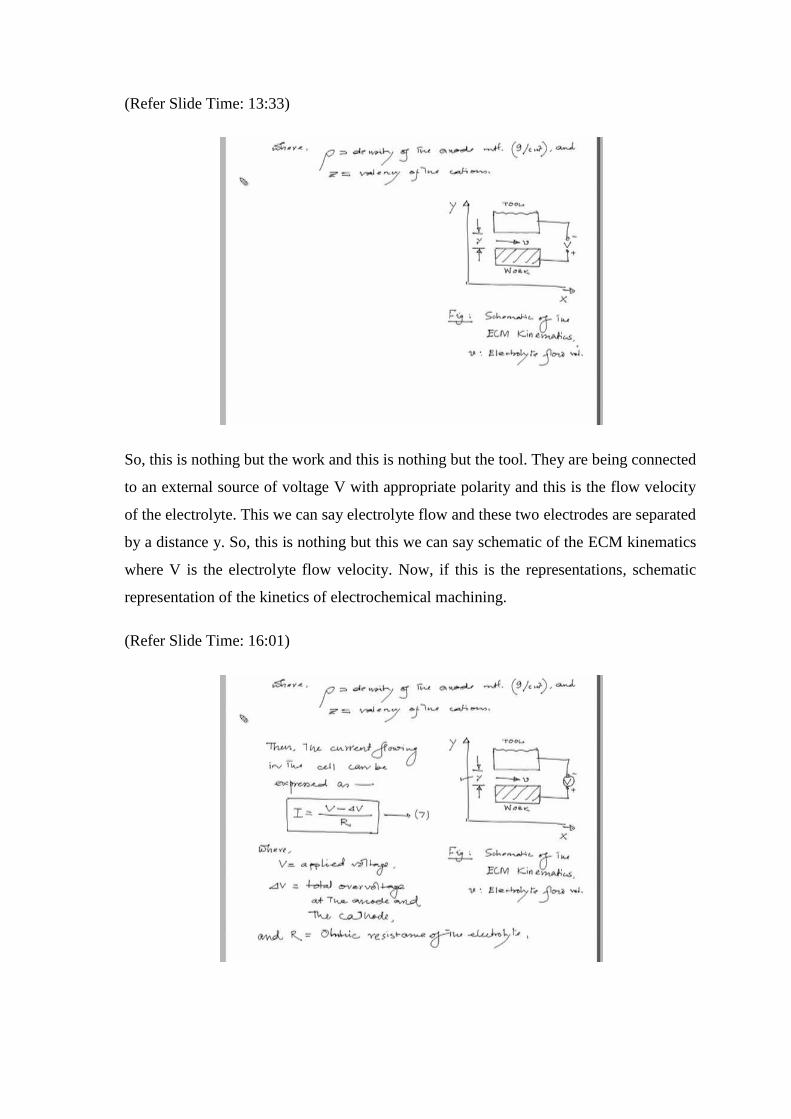
So, this is nothing but the work and this is nothing but the tool. They are being connected
to an external source of voltage V with appropriate polarity and this is the flow velocity
of the electrolyte. This we can say electrolyte flow and these two electrodes are separated
by a distance y. So, this is nothing but this we can say schematic of the ECM kinematics
where V is the electrolyte flow velocity. Now, if this is the representations, schematic
representation of the kinetics of electrochemical machining.
(Refer Slide Time: 16:01)

Then the current flowing in the cell, then the current flowing in the cell can be expressed
as I is V minus del V by R where this equation can be expressed or numbered as seven
keeping the continuation where V is nothing but our applied voltage. This we have
shown here, V is applied voltage and then del V is total over voltage at the anode and the
cathode and R is the ohmic resistance. Now, if the electrolytes are separated by a
distance y as as shown here this y then the current density.
(Refer Slide Time: 18:25)
Now, the current density which is conventionally expressed by the symbol J through the
electrolyte can be expressed as J is equal to kappa V minus del V divided by y. Let us
call this as equation eight where y is the distance between the electrodes and kappa is the
conductivity of the electrolyte.
(Refer Slide Time: 19:59)
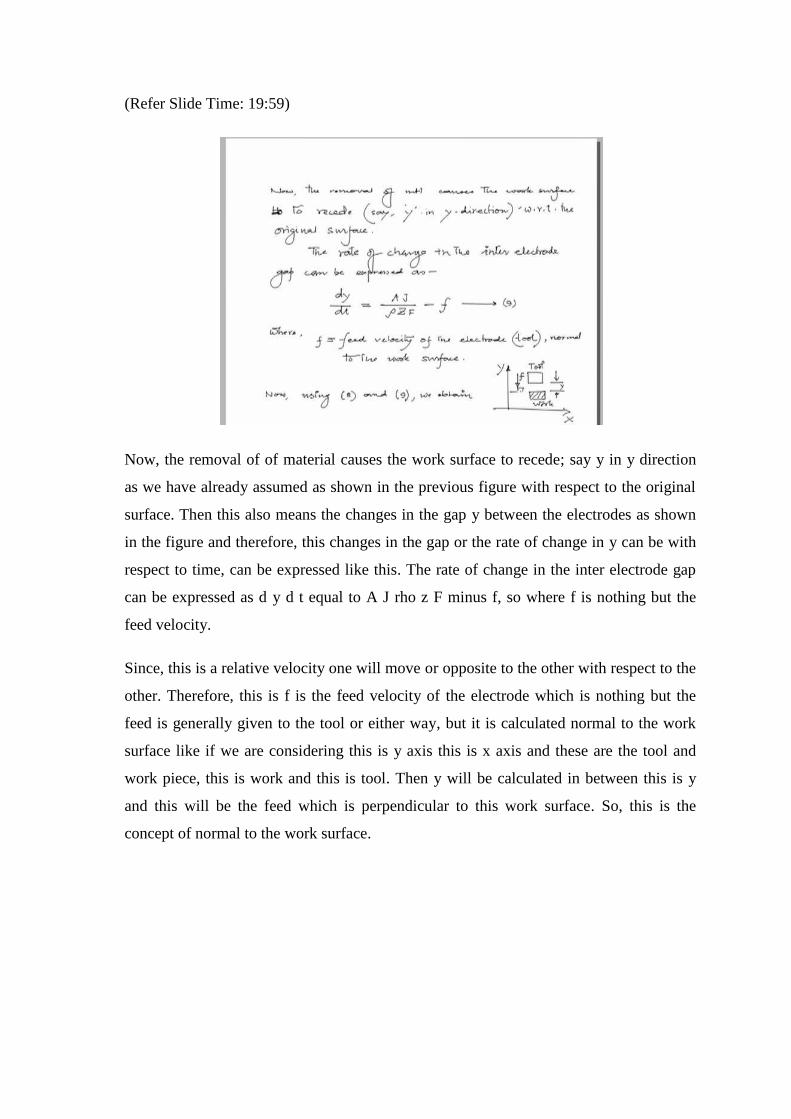
Now, the removal of of material causes the work surface to recede; say y in y direction
as we have already assumed as shown in the previous figure with respect to the original
surface. Then this also means the changes in the gap y between the electrodes as shown
in the figure and therefore, this changes in the gap or the rate of change in y can be with
respect to time, can be expressed like this. The rate of change in the inter electrode gap
can be expressed as d y d t equal to A J rho z F minus f, so where f is nothing but the
feed velocity.
Since, this is a relative velocity one will move or opposite to the other with respect to the
other. Therefore, this is f is the feed velocity of the electrode which is nothing but the
feed is generally given to the tool or either way, but it is calculated normal to the work
surface like if we are considering this is y axis this is x axis and these are the tool and
work piece, this is work and this is tool. Then y will be calculated in between this is y
and this will be the feed which is perpendicular to this work surface. So, this is the
concept of normal to the work surface.

(Refer Slide Time: 24:21)
Now, using the previous equation that is eight and this recent equation that is nine we
obtain that d y d t is kappa times A V minus del V rho Z F, this is 1 upon y minus f. On
simplification we can write d y d t is equal to sigma by y minus f. This is the simplified
form say let us say this is equation ten in which where we have represented or brought in
one new term that is sigma and sigma can is expressed as kappa times A into V minus
del V divided by rho Z and F. V minus del V as we have already indicated V is the
applied voltage and del V is the over voltage therefore, difference between this voltage
and over voltage will be the net voltage or effective voltage that will be responsible for
the current flowing in the circuit, that is I and corresponding current density will be Z,
with this background, this we can say as our background study.

(Refer Slide Time: 26:10)
Now, we will move into the tool design aspect. Generally, there are two aspects in ECM
tool design, one is the determination of the tool shape or the equation of the tool and
other aspect is the, given the work surface, work profile designing of the other things like
gap etcetera. There are two aspects, we can say tool design, one we can say determining
the tool shape in order to achieve the required job profile.
The other aspect is determining the tool for other conditions. This other conditions may
be say flow of electrolyte, say flow of electrolyte, strength etcetera. Now, here let us
consider the primary task of determining the tool shape. We will mostly consider the
determination of the tools that is in terms of a mathematical equation. Let us consider the
cos theta method.(Refer Slide Time: 28:58)

Say this is our tool and this is our work piece. This is the cathode or also known as tool
and this is the anode also known as the work. Now, distance between them let us call this
as the inter electrode gap height as h e. Now, this can be, the distance between them can
be mathematically derived like this. If this is angle theta then this is also theta,
mathematically you can say. Then this distance can be expressed as h e by cos theta, this
is on the work surface as we have seen, this is the work surface.
Therefore, the distance between this can be at any instant during machining can be
expressed as h e by cos theta. Now, let us consider in this way. We are operating inside a
frame of x and y and as usual this is the cathode which is the tool itself and this is the
anode which is nothing but the work. Now, as I already indicated this is, let us consider
this as the feed direction which is along the y axis and this is relative to the tool and work
piece. Therefore, this is the feed direction and let us consider two points on the surfaces
say this is point B and this is point A. A is having the coordinate let us consider as x w
that is for w for work and y w.
Similarly, for the point B on the tool let us consider the coordinate of this point given by
x t, t stands for the tool and y t, that means during machining this tool is either coming
towards this work or the work is being fed towards the tool which constitutes the feed.
That means this we can consider as theta and let us consider this work profile is given by
the function y equal to phi of x. Now, the equilibrium gap between the anode and the
cathode surface that is as we have already shown in the figure that is nothing but this h e
can be expressed mathematically as…

(Refer Slide Time: 35:23)
h e is nothing but kappa A then the effective voltage between the electrodes divided by
the density, then valency, then the Faraday’s constant, then f of cos theta. Let us consider
this as equation number eleven where as I have already explained V is nothing but the
applied voltage, del V is the over voltage, f is the feed rate and theta is the inclination of
the of the feed direction to the surface normal.
(Refer Slide Time: 37:15)
Here it is to be noted that the feed direction is considered parallel to the y axis. This in
the pictorial representation also in the scheme also we have shown, this is feed is parallel
to the y direction. Let us consider the following for the analysis.
(Refer Slide Time: 38:15)
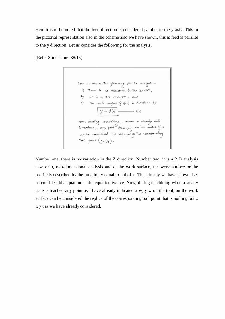
Number one, there is no variation in the Z direction. Number two, it is a 2 D analysis
case or b, two-dimensional analysis and c, the work surface, the work surface or the
profile is described by the function y equal to phi of x. This already we have shown. Let
us consider this equation as the equation twelve. Now, during machining when a steady
state is reached any point as I have already indicated x w, y w on the tool, on the work
surface can be considered the replica of the corresponding tool point that is nothing but x
t, y t as we have already considered.
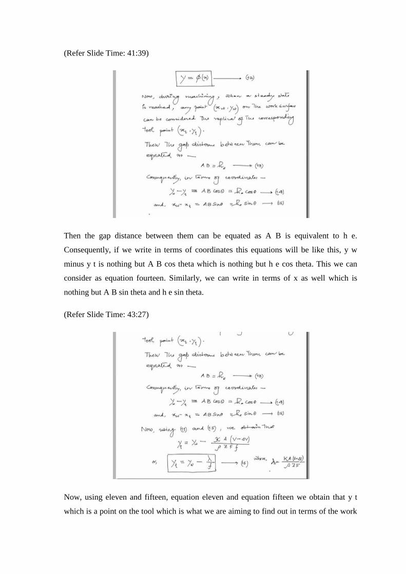
(Refer Slide Time: 41:39)
Then the gap distance between them can be equated as A B is equivalent to h e.
Consequently, if we write in terms of coordinates this equations will be like this, y w
minus y t is nothing but A B cos theta which is nothing but h e cos theta. This we can
consider as equation fourteen. Similarly, we can write in terms of x as well which is
nothing but A B sin theta and h e sin theta.
(Refer Slide Time: 43:27)
Now, using eleven and fifteen, equation eleven and equation fifteen we obtain that y t
which is a point on the tool which is what we are aiming to find out in terms of the work
piece coordinate and kappa times A, this is what we are replacing this divided by rho Z F
and small f or this can be written as y t equal to y w minus sigma by small f. This we can
consider as equation sixteen which will be an important relationship in future. So, here
we have replaced this term K kappa into V minus del V divided by rho Z and capital f by
the term sigma.
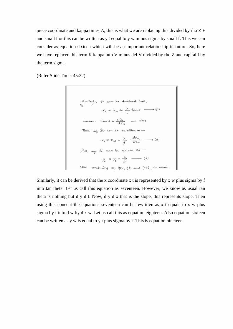
(Refer Slide Time: 45:22)
Similarly, it can be derived that the x coordinate x t is represented by x w plus sigma by f
into tan theta. Let us call this equation as seventeen. However, we know as usual tan
theta is nothing but d y d t. Now, d y d x that is the slope, this represents slope. Then
using this concept the equations seventeen can be rewritten as x t equals to x w plus
sigma by f into d w by d x w. Let us call this as equation eighteen. Also equation sixteen
can be written as y w is equal to y t plus sigma by f. This is equation nineteen.

(Refer Slide Time: 48:11)
Now, combining equation twelve, eighteen and nineteen we obtained y t plus sigma by f
equal to y w. This is in terms of phi x t minus sigma by f into d phi x w, d x w. On
simplification this will yield y t equal to phi of x t minus sigma by small f psi of x t y t
minus the other term sigma by f. Let us consider this as equation twenty. However, here
we have brought in a new term that is psi of x t y t, this is nothing but d phi x w by d x w
is expressed in terms of tool coordinates as a function psi of x t y t.
(Refer Slide Time: 50:26)

Hence, the tool surface geometry can be expressed using equation twenty as y equal to
phi of x minus lambda by small f, then psi of x y minus lambda by small f, this is
generalized equation. So, this equation will describe in general the tool profile that is y is
equal to; y is nothing but the coordinate in the tool profile. And then it is a function of
phi of x minus sigma by f function of x and y that is psi of x and y minus sigma by small
f, that is in terms of feed, small f is nothing but feed. This describes the tool equation in
case of ECM tool design.
Thus, in this session we have discussed about the designing of ECM tool. We have
freshened ourselves with the basics of electrochemical machining, the governing laws,
that is Faraday’s laws of electrochemical dissociation and which are used in
electrochemical machining and then we have seen the simple kinematics that is involved
in electrochemical machining and then we have derived a tool equation which represents
the tool for the corresponding profile and work and can be used for designing the tool.
That describes the tool shape in terms of the work piece function. We hope the session
was informative and interesting.
Thank you.