advanced search - university of...
TRANSCRIPT
slide 1
Advanced Search Hill climbing, simulated annealing,
genetic algorithm
Xiaojin Zhu
Computer Sciences Department
University of Wisconsin, Madison
[Based on slides from Andrew Moore http://www.cs.cmu.edu/~awm/tutorials ]

slide 2
Optimization problems
• Previously we want a path from start to goal
Uninformed search: g(s): Iterative Deepening
Informed search: g(s)+h(s): A*
• Now a different setting:
Each state s has a score f(s) that we can compute
The goal is to find the state with the highest score, or
a reasonably high score
Do not care about the path
This is an optimization problem
Enumerating the states is intractable
Even previous search algorithms are too expensive
slide 3
Examples
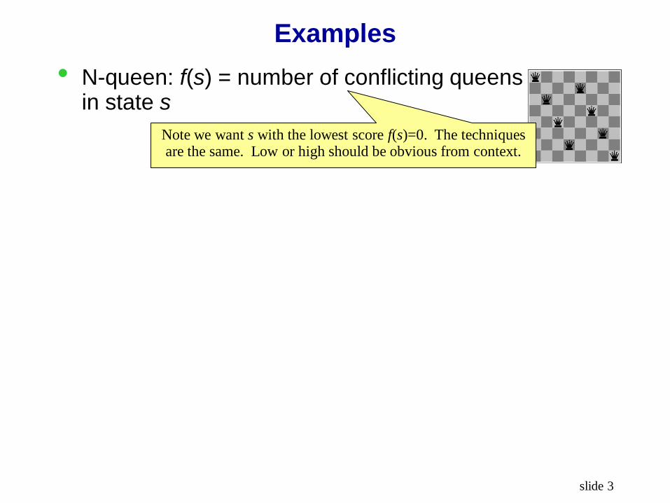
• N-queen: f(s) = number of conflicting queens in state s
Note we want s with the lowest score f(s)=0. The techniques are the same. Low or high should be obvious from context.
slide 4
Examples
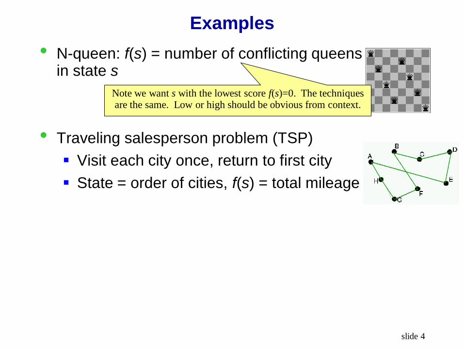
• N-queen: f(s) = number of conflicting queens in state s
• Traveling salesperson problem (TSP)
Visit each city once, return to first city
State = order of cities, f(s) = total mileage
Note we want s with the lowest score f(s)=0. The techniques are the same. Low or high should be obvious from context.

slide 5
Examples
• N-queen: f(s) = number of conflicting queens in state s
• Traveling salesperson problem (TSP)
Visit each city once, return to first city
State = order of cities, f(s) = total mileage
• Boolean satisfiability (e.g., 3-SAT)
State = assignment to variables
f(s) = # satisfied clauses
Note we want s with the lowest score f(s)=0. The techniques are the same. Low or high should be obvious from context.
A B C
A C D
B D E
C D E
A C E

slide 6
1. HILL CLIMBING
slide 7
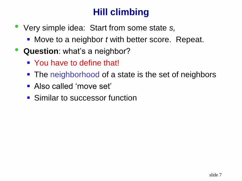
Hill climbing
• Very simple idea: Start from some state s,
Move to a neighbor t with better score. Repeat.
• Question: what’s a neighbor?
You have to define that!
The neighborhood of a state is the set of neighbors
Also called ‘move set’
Similar to successor function
slide 8
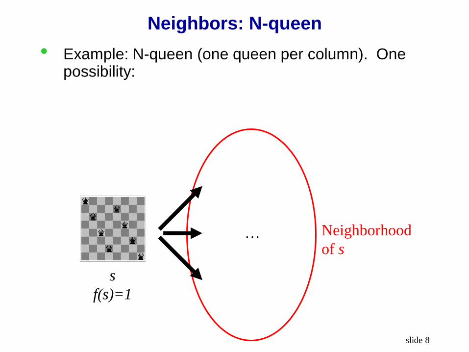
Neighbors: N-queen
• Example: N-queen (one queen per column). One possibility:
…
s
f(s)=1
Neighborhood
of s
slide 9
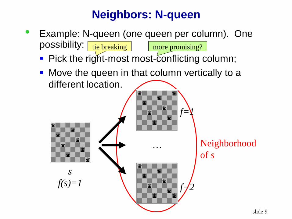
Neighbors: N-queen
• Example: N-queen (one queen per column). One possibility:
Pick the right-most most-conflicting column;
Move the queen in that column vertically to a
different location.
…
s
f(s)=1
Neighborhood
of s
f=1
f=2
tie breaking more promising?

slide 10
Neighbors: TSP
• state: A-B-C-D-E-F-G-H-A
• f = length of tour

slide 11
Neighbors: TSP
• state: A-B-C-D-E-F-G-H-A
• f = length of tour
• One possibility: 2-change
A-B-C-D-E-F-G-H-A
A-E-D-C-B-F-G-H-A
flip
slide 12
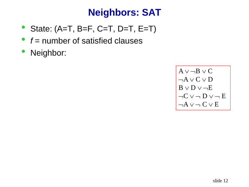
Neighbors: SAT
• State: (A=T, B=F, C=T, D=T, E=T)
• f = number of satisfied clauses
• Neighbor:
A B C
A C D
B D E
C D E
A C E
slide 13
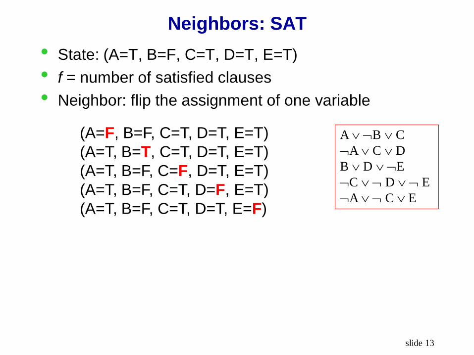
Neighbors: SAT
• State: (A=T, B=F, C=T, D=T, E=T)
• f = number of satisfied clauses
• Neighbor: flip the assignment of one variable
A B C
A C D
B D E
C D E
A C E
(A=F, B=F, C=T, D=T, E=T)
(A=T, B=T, C=T, D=T, E=T)
(A=T, B=F, C=F, D=T, E=T)
(A=T, B=F, C=T, D=F, E=T)
(A=T, B=F, C=T, D=T, E=F)

slide 14
Hill climbing
• Question: What’s a neighbor?
(vaguely) Problems tend to have structures. A small
change produces a neighboring state.
The neighborhood must be small enough for
efficiency
Designing the neighborhood is critical. This is the
real ingenuity – not the decision to use hill climbing.
• Question: Pick which neighbor?
• Question: What if no neighbor is better than the
current state?

slide 15
Hill climbing
• Question: What’s a neighbor?
(vaguely) Problems tend to have structures. A small
change produces a neighboring state.
The neighborhood must be small enough for
efficiency
Designing the neighborhood is critical. This is the
real ingenuity – not the decision to use hill climbing.
• Question: Pick which neighbor? The best one (greedy)
• Question: What if no neighbor is better than the
current state? Stop. (Doh!)
slide 16
Hill climbing algorithm
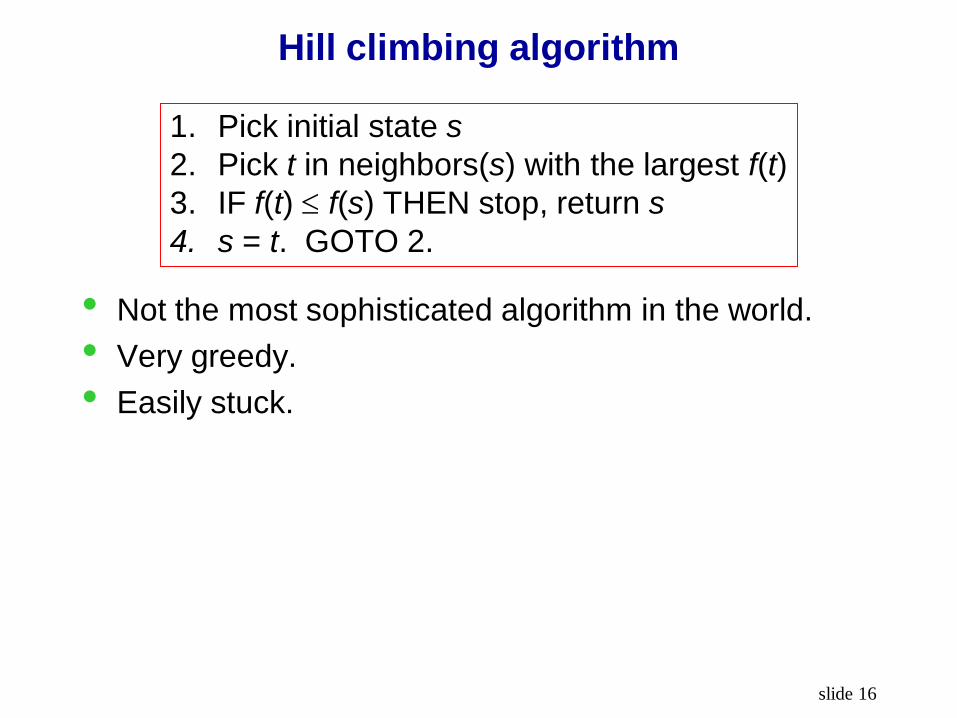
1. Pick initial state s
2. Pick t in neighbors(s) with the largest f(t)
3. IF f(t) f(s) THEN stop, return s
4. s = t. GOTO 2.
• Not the most sophisticated algorithm in the world.
• Very greedy.
• Easily stuck.
slide 17
Hill climbing algorithm
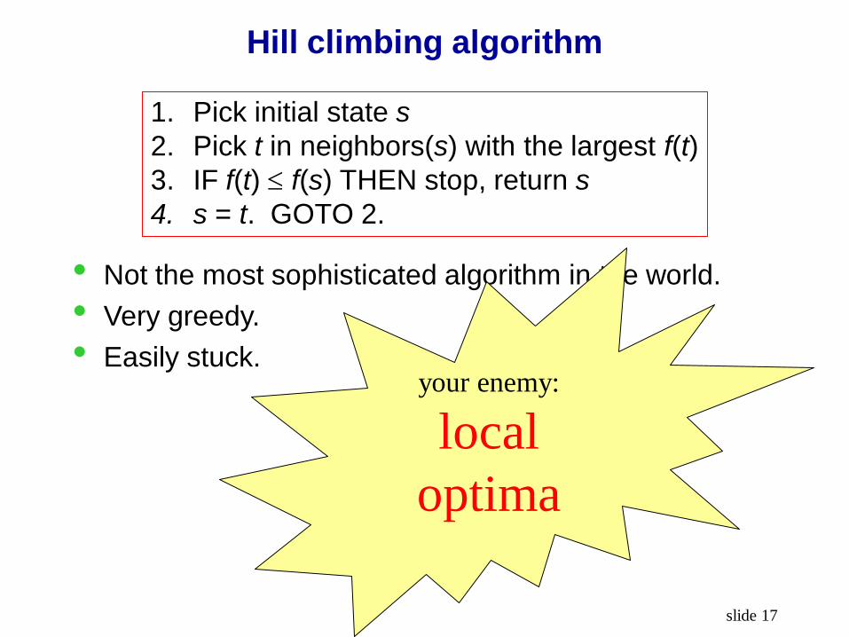
1. Pick initial state s
2. Pick t in neighbors(s) with the largest f(t)
3. IF f(t) f(s) THEN stop, return s
4. s = t. GOTO 2.
• Not the most sophisticated algorithm in the world.
• Very greedy.
• Easily stuck.
your enemy:
local
optima
slide 18
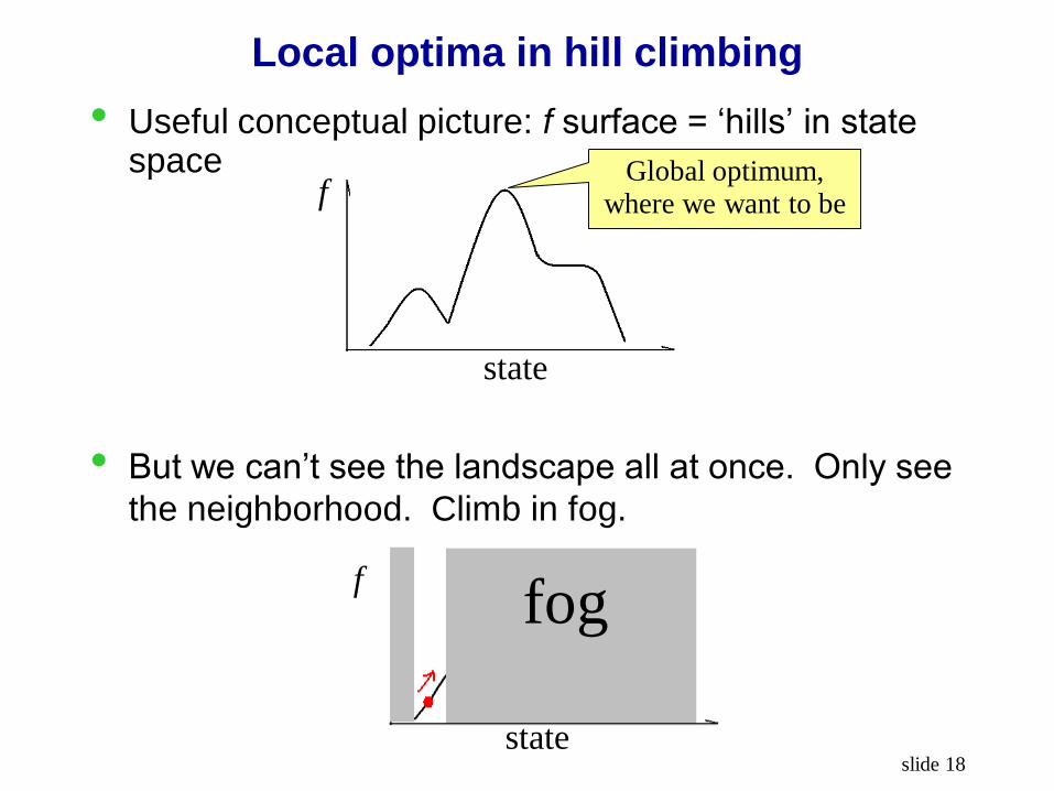
Local optima in hill climbing
• Useful conceptual picture: f surface = ‘hills’ in state space
• But we can’t see the landscape all at once. Only see
the neighborhood. Climb in fog.
state
f Global optimum,
where we want to be
state
f fog

slide 19
Local optima in hill climbing
• Local optima (there can be many!)
• Plateaux
Declare top-of-the-world?
state
f
state
f Where shall I go?

slide 20
Local optima in hill climbing
• Local optima (there can be many!)
• Plateaus
fog Declare top of
the world?
state
f
state
f
fog
Where shall I go?
The rest of the lecture is about
Escaping
local optima

slide 21
Not every local minimum should be escaped

slide 22
Repeated hill climbing with random restarts
• Very simple modification
1. When stuck, pick a random new start, run basic
hill climbing from there.
2. Repeat this k times.
3. Return the best of the k local optima.
• Can be very effective
• Should be tried whenever hill climbing is used

slide 23
Variations of hill climbing
• Question: How do we make hill climbing less greedy?
slide 24
Variations of hill climbing
• Question: How do we make hill climbing less greedy?
Stochastic hill climbing
• Randomly select among better neighbors
• The better, the more likely
• Pros / cons compared with basic hill climbing?

slide 25
Variations of hill climbing
• Question: How do we make hill climbing less greedy?
Stochastic hill climbing
• Randomly select among better neighbors
• The better, the more likely
• Pros / cons compared with basic hill climbing?
• Question: What if the neighborhood is too large to enumerate? (e.g. N-queen if we need to pick both the column and the move within it)
slide 26
Variations of hill climbing
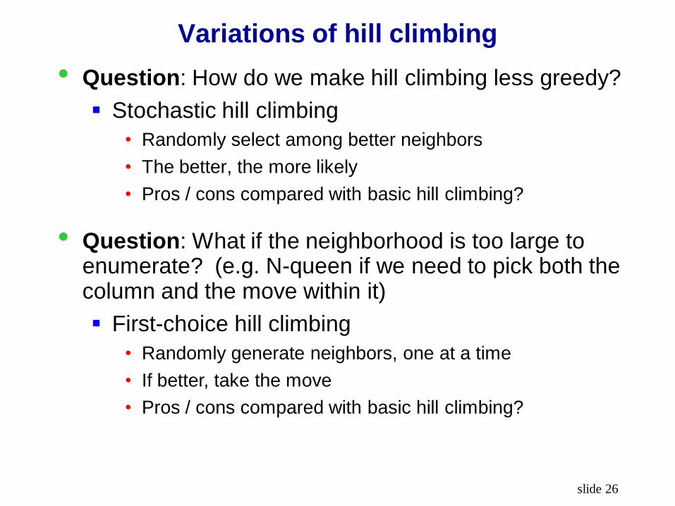
• Question: How do we make hill climbing less greedy?
Stochastic hill climbing
• Randomly select among better neighbors
• The better, the more likely
• Pros / cons compared with basic hill climbing?
• Question: What if the neighborhood is too large to enumerate? (e.g. N-queen if we need to pick both the column and the move within it)
First-choice hill climbing
• Randomly generate neighbors, one at a time
• If better, take the move
• Pros / cons compared with basic hill climbing?
slide 27
Variations of hill climbing
• We are still greedy! Only willing to move upwards.
• Important observation in life:
Sometimes one needs to temporarily step back in order to move forward.
Sometimes one needs to move to an inferior neighbor in order to escape a local optimum.
=
slide 28
Variations of hill climbing
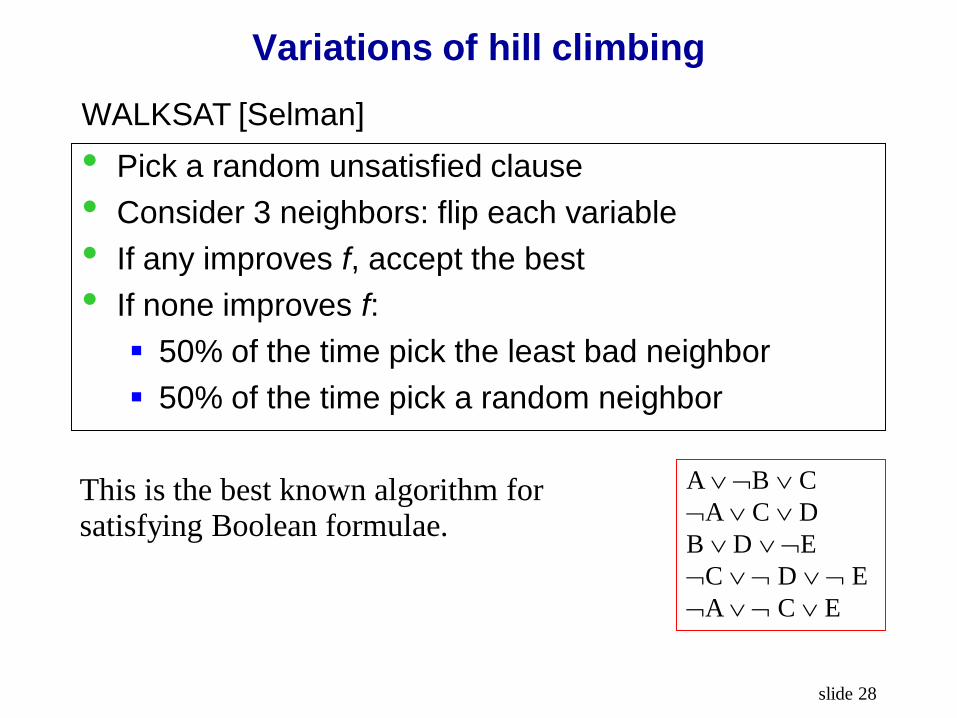
• Pick a random unsatisfied clause
• Consider 3 neighbors: flip each variable
• If any improves f, accept the best
• If none improves f:
50% of the time pick the least bad neighbor
50% of the time pick a random neighbor
A B C
A C D
B D E
C D E
A C E
WALKSAT [Selman]
This is the best known algorithm for satisfying Boolean formulae.
slide 29
2. SIMULATED ANNEALING

slide 30
Simulated Annealing
anneal
• To subject (glass or metal) to a process of heating
and slow cooling in order to toughen and reduce
brittleness.

slide 31
Simulated Annealing
1. Pick initial state s
2. Randomly pick t in neighbors(s)
3. IF f(t) better THEN accept st.
4. ELSE /* t is worse than s */
5. accept st with a small probability
6. GOTO 2 until bored.

slide 32
Simulated Annealing
1. Pick initial state s
2. Randomly pick t in neighbors(s)
3. IF f(t) better THEN accept st.
4. ELSE /* t is worse than s */
5. accept st with a small probability
6. GOTO 2 until bored.
How to choose the small probability?
idea 1: p = 0.1

slide 33
Simulated Annealing
1. Pick initial state s
2. Randomly pick t in neighbors(s)
3. IF f(t) better THEN accept st.
4. ELSE /* t is worse than s */
5. accept st with a small probability
6. GOTO 2 until bored.
How to choose the small probability?
idea 1: p = 0.1
idea 2: p decreases with time

slide 34
Simulated Annealing
1. Pick initial state s
2. Randomly pick t in neighbors(s)
3. IF f(t) better THEN accept st.
4. ELSE /* t is worse than s */
5. accept st with a small probability
6. GOTO 2 until bored.
How to choose the small probability?
idea 1: p = 0.1
idea 2: p decreases with time
idea 3: p decreases with time, also as the ‘badness’
|f(s)-f(t)| increases
slide 35
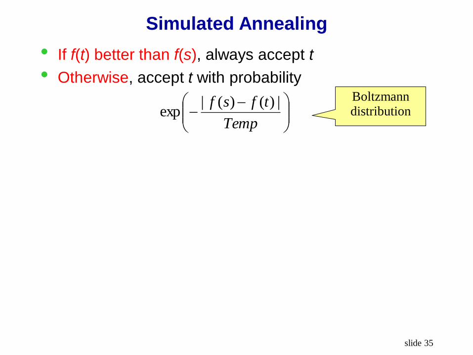
Simulated Annealing
• If f(t) better than f(s), always accept t
• Otherwise, accept t with probability
Boltzmann distribution
Temp
tfsf |)()(|exp

slide 36
Simulated Annealing
• If f(t) better than f(s), always accept t
• Otherwise, accept t with probability
• Temp is a temperature parameter that ‘cools’
(anneals) over time, e.g. TempTemp*0.9 which
gives Temp=(T0)#iteration
High temperature: almost always accept any t
Low temperature: first-choice hill climbing
• If the ‘badness’ (formally known as energy difference)
|f(s)-f(t)| is large, the probability is small.
Boltzmann distribution
Temp
tfsf |)()(|exp
slide 37
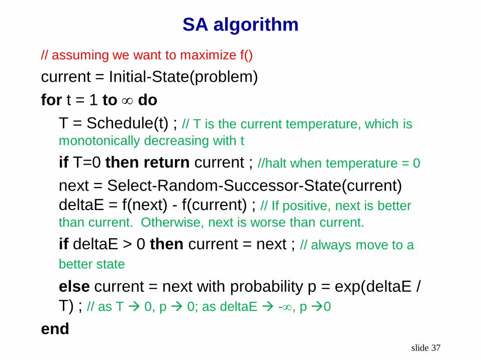
SA algorithm
// assuming we want to maximize f()
current = Initial-State(problem)
for t = 1 to do
T = Schedule(t) ; // T is the current temperature, which is
monotonically decreasing with t
if T=0 then return current ; //halt when temperature = 0
next = Select-Random-Successor-State(current)
deltaE = f(next) - f(current) ; // If positive, next is better
than current. Otherwise, next is worse than current.
if deltaE > 0 then current = next ; // always move to a
better state
else current = next with probability p = exp(deltaE /
T) ; // as T 0, p 0; as deltaE -, p 0
end
slide 38
Simulated Annealing issues
• Cooling scheme important
• Neighborhood design is the real ingenuity, not the
decision to use simulated annealing.
• Not much to say theoretically
With infinitely slow cooling rate, finds global
optimum with probability 1.
• Proposed by Metropolis in 1953 based on the
analogy that alloys manage to find a near global
minimum energy state, when annealed slowly.
• Easy to implement.
• Try hill-climbing with random restarts first!

slide 39
GENETIC ALGORITHM
http://www.genetic-programming.org/

slide 40
Evolution
• Survival of the fittest, a.k.a. natural selection
• Genes encoded as DNA (deoxyribonucleic acid), sequence of
bases: A (Adenine), C (Cytosine), T (Thymine) and G (Guanine)
• The chromosomes from the parents exchange randomly by a
process called crossover. Therefore, the offspring exhibit some
traits of the father and some traits of the mother.
Requires genetic diversity among the parents to ensure
sufficiently varied offspring
• A rarer process called mutation also changes the genes (e.g.
from cosmic ray).
Nonsensical/deadly mutated organisms die.
Beneficial mutations produce “stronger” organisms
Neither: organisms aren’t improved.

slide 41
Natural selection
• Individuals compete for resources
• Individuals with better genes have a larger chance to
produce offspring, and vice versa
• After many generations, the population consists of
lots of genes from the superior individuals, and less
from the inferior individuals
• Superiority defined by fitness to the environment
• Popularized by Darwin
• Mistake of Lamarck: environment does not force an
individual to change its genes

slide 42
Genetic algorithm
• Yet another AI algorithm based on real-world analogy
• Yet another heuristic stochastic search algorithm
• Each state s is called an individual. Often (carefully)
coded up as a string.
• The score f(s) is called the fitness of s. Our goal is to
find the global optimum (fittest) state.
• At any time we keep a fixed number of states. They
are called the population. Similar to beam search.
(3 2 7 5 2 4 1 1)

slide 43
Individual encoding
• The “DNA”
• Satisfiability problem
(A B C D E) = (T F T T T)
• TSP
A B C
A C D
B D E
C D E
A C E A-E-D-C-B-F-G-H-A
slide 44
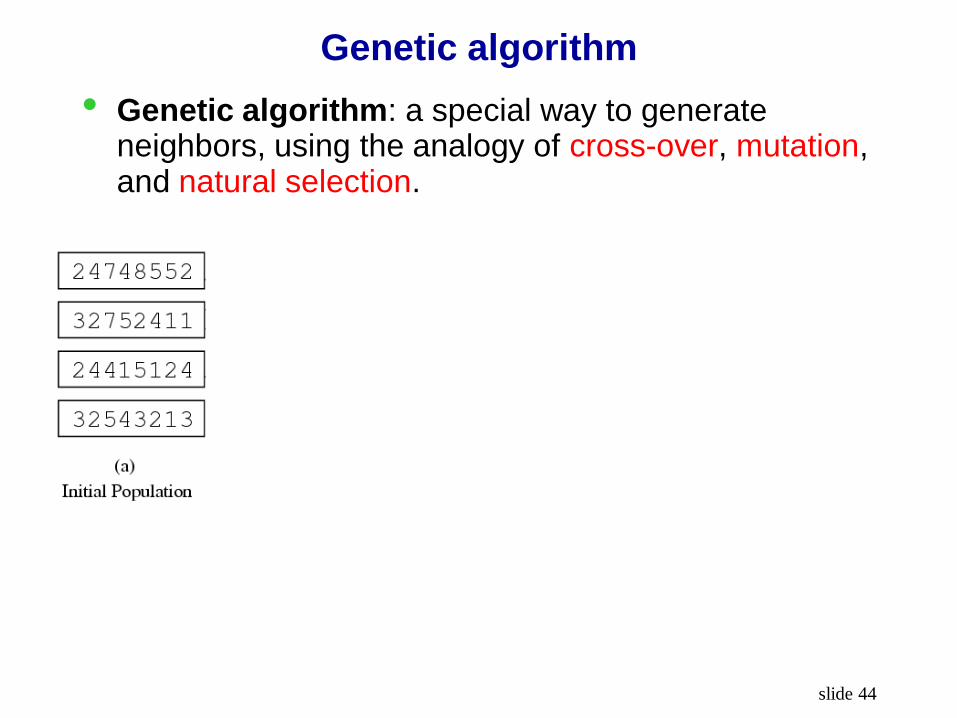
Genetic algorithm
• Genetic algorithm: a special way to generate neighbors, using the analogy of cross-over, mutation, and natural selection.
slide 45
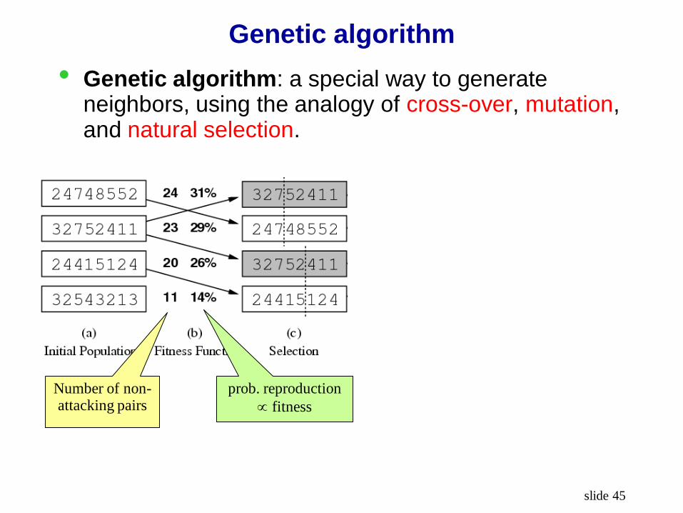
Genetic algorithm
• Genetic algorithm: a special way to generate neighbors, using the analogy of cross-over, mutation, and natural selection.
Number of non-attacking pairs
prob. reproduction
fitness

slide 46
Genetic algorithm
• Genetic algorithm: a special way to generate neighbors, using the analogy of cross-over, mutation, and natural selection.
Number of non-attacking pairs
prob. reproduction
fitness
Next generation

slide 47
Genetic algorithm
• Genetic algorithm: a special way to generate neighbors, using the analogy of cross-over, mutation, and natural selection.
Number of non-attacking pairs
prob. reproduction
fitness
Next generation

slide 48
Genetic algorithm (one variety)
1. Let s1, …, sN be the current population
2. Let pi = f(si) / j f(sj) be the reproduction probability
3. FOR k = 1; k<N; k+=2
• parent1 = randomly pick according to p
• parent2 = randomly pick another
• randomly select a crossover point, swap strings
of parents 1, 2 to generate children t[k], t[k+1]
4. FOR k = 1; k<=N; k++
• Randomly mutate each position in t[k] with a
small probability (mutation rate)
5. The new generation replaces the old: { s }{ t }.
Repeat.

slide 49
Proportional selection
• pi = f(si) / j f(sj)
• j f(sj) = 5+20+11+8+6=50
• p1=5/50=10%

slide 50
Variations of genetic algorithm
• Parents may survive into the next generation
• Use ranking instead of f(s) in computing the
reproduction probabilities.
• Cross over random bits instead of chunks.
• Optimize over sentences from a programming
language. Genetic programming.
• …
slide 51
Genetic algorithm issues
• State encoding is the real ingenuity, not the decision to use genetic algorithm.
• Lack of diversity can lead to premature convergence and non-optimal solution
• Not much to say theoretically
Cross over (sexual reproduction) much more
efficient than mutation (asexual reproduction).
• Easy to implement.
• Try hill-climbing with random restarts first!