advanced techniques to increase the lifetime of smart...
TRANSCRIPT

Deliverable D4.2
Advanced techniques to increase the lifetime of smart objects and ensure low power network operation
Editor: George Oikonomou, UNIVBRIS
Deliverable nature: Report (R)
Dissemination level: (Confidentiality)
Public (PU)
Contractual delivery date: 31 Aug 2015
Actual delivery date: 4 September 2015
Suggested readers: Researchers, IERC, application developers, system administrators
Version: 1.0
Total number of pages: 119
Keywords: Internet of Things, Reliability, Availability, Compressive Sensing, Heterogeneous Networks, Matrix Completion, Congestion-Aware Radio Duty Cycling, Energy-Aware Relays, 6LoWPAN Multicast Forwarding, Multi-Radio Selection, Security / Power Consumption Trade-Offs, Low-Power Hardware
Abstract
This document presents the results of the work undertaken as part of Task 4.3 “Energy efficient operation”. The algorithms and mechanisms developed and investigated here aim to increase the lifetime of a RERUM Device deployment and to improve system availability. Most of the research is applicable on RDs, but some research results for gateways are also included in this deliverable. Energy consumption has been analysed and optimised from multiple different angles, namely: i) Data gathering and transmission using Compressive Sensing is used in order to reduce the frequency of data transmission and reduce the need for retransmissions in case of lost packets. ii) Sleep and Wake-Up techniques are used to reduce idle radio listening, a major cause of battery drain, to reduce network congestion and to improve gateway energy-awareness. iii) Novel networking algorithms and protocols are proposed to improve the performance of IPv6 multicast forwarding and to optimise multi-radio selection mechanisms. iv) The trade-off between security and energy-efficiency is analysed for authorisation and digital signature mechanisms. v) We analyse hardware and software-related design decisions influencing the energy consumption of the RERUM-developed RE-Mote sensor platform. With the exception of the discussion on the RE-Mote platform, most of the mechanisms presented in this deliverable have been investigated analytically or through simulations. Some of those mechanisms will be further evaluated in a lab environment and RERUM’s field trials as part of WP5.
Ref. Ares(2015)3669911 - 07/09/2015

RERUM FP7-ICT-609094 Deliverable D4.2
Disclaimer
This document contains material, which is the copyright of certain RERUM consortium parties, and may not be reproduced or copied without permission.
All RERUM consortium parties have agreed to full publication of this document.
The commercial use of any information contained in this document may require a license from the proprietor of that information.
Neither the RERUM consortium as a whole, nor a certain part of the RERUM consortium, warrant that the information contained in this document is capable of use, nor that use of the information is free from risk, accepting no liability for loss or damage suffered by any person using this information.
The research leading to these results has received funding from the European Union's Seventh Framework Programme (FP7/2007-2013) under grant agreement n° 609094.
Page 2 of (119) © RERUM consortium members 2015

Deliverable D4.2 RERUM FP7-ICT-609094
Impressum
Full project title Reliable, resilient and secure IoT for smart city applications
Short project title RERUM
Number and title of work-package WP4 - Reliability, availability, robustness and scalability
Number and title of task T4.3 – Energy efficient operation
Document title Advanced techniques to increase the lifetime of smart objects and ensure low power network operation
Editor: Name, company George Oikonomou, UNIVBRIS
Work-package leader: Name, company Elias Tragos, FORTH
Estimation of person months (PMs) spent on the Deliverable
Copyright notice
2015 Participants in project RERUM
This work is licensed under the Creative Commons Attribution-NonCommercial-NoDerivs 3.0 Unported License. To view a copy of this license, visit http://creativecommons.org/licenses/by-nc-nd/3.0
© RERUM consortium members 2015 Page 3 of (119)

RERUM FP7-ICT-609094 Deliverable D4.2
Executive summary This deliverable presents techniques developed within the RERUM project for increasing the lifetime of a RERUM use-case deployment by optimising the energy consumption of REDUM Devices and gateways. Some of the techniques presented here also improve network performance and availability by decreasing message transmission delays and packet losses. This deliverable (D4.2) is the output of the activities of Task 4.3 “Energy-Efficient Operation” within Work Package 4 (WP4) “Reliability, availability, robustness and scalability”.
Some of the techniques discussed have been developed as part of previous RERUM Tasks (T3.2, T4.1, T4.2), whereas some of them are entirely novel. RERUM’s requirements in terms of RD energy consumption were first presented in D2.2, and the content of this deliverable informed the progress of Task 4.3 that is documented here.
In this respect, the following techniques are analysed in this deliverable:
Energy-Efficient Data Gathering and Transmission Using Compressive Sensing: Analysis of RERUM-developed techniques that can extend the battery lifetime of constrained devices by minimising the frequency of data sampling and their transmissions, both of which are energy-consuming tasks.
Sleep and Wake-Up Techniques: We discuss two methods. The first one focuses on duty-cycled radio operation with congestion-awareness. The second method explores novel techniques to improve the energy awareness of RERUM gateways that act as relays between a number of RDs and a destination.
Networking algorithms and protocols: We present an analysis of the energy consumption properties of a multicast forwarding algorithm for IPv6-based low-power wireless networks. We also evaluate an energy-efficient multi-radio selection mechanism based on a scheme named “threshold-based selection diversity”.
Trade-offs between Security and Energy-Efficiency: We investigate security and energy consumption trade-offs for a RERUM-developed privacy-preserving authorization mechanism and for the JSON Signatures Scheme (JSS) that was developed by RERUM and was first presented in D3.1.
Hardware design and component selection, alongside accompanying software: We present real power consumption measurements in a lab environment using the first and second prototypes of the RERUM-manufactured RE-Mote platform. The discussion includes hardware design decisions and software optimisations.
The techniques presented here have been published in academic conferences [APA15, CFT15, FCT14, FTPC14, LM14, MOPG14]. The RERUM-developed privacy-preserving authorization mechanism was recently resented at the IETF’s Authentication and Authorization for Constrained Environments (ACE) working group.
The purely technical nature and scientific of this deliverable may create difficulties to non-expert readers; thus, an introductory part is included at the beginning of each section describing briefly (i) the motivation for developing each technique, (ii) the relation with the RERUM Use Cases and the practical problem the technique tries to solve.
Page 4 of (119) © RERUM consortium members 2015

Deliverable D4.2 RERUM FP7-ICT-609094
List of Authors Company Author Contribution
SAG Jorge Cuellar Power consumption evaluation of authorization mechanisms
UNIVBRIS George Oikonomou
Congestion Aware Duty Cycling RDs in 6LoWPANs
Energy consumption of multicast forwarding with BMFA
Contiki’s Low-Power Module
LiU Vangelis Angelakis, Ioannis Avgouleas, Anthony Ephremides
Energy-aware relay properties of gateways
Zolertia Antonio Liñán Low-Power Hardware Design Characteristics
RE-Mote Contiki power consumption measurements
FORTH
Alexandros Fragkiadakis Elias Tragos Pavlos Charalampidis George Stamatakis
Minimization of Data Sampling and Transmission using Compressive Sensing
CYTA Athanasios Lioumpas
Adaptive and energy-efficient multi-radio selection mechanisms
Energy consumption of the JSON Signature Scheme
© RERUM consortium members 2015 Page 5 of (119)

RERUM FP7-ICT-609094 Deliverable D4.2
Table of Contents Executive summary ................................................................................................................................. 4
Table of Contents .................................................................................................................................... 6
List of Figures ........................................................................................................................................... 9
List of Tables .......................................................................................................................................... 12
List of Snippets ...................................................................................................................................... 13
Abbreviations ........................................................................................................................................ 14
Definitions ............................................................................................................................................. 16
1 Introduction ................................................................................................................................... 20
1.1 Intended audience ................................................................................................................. 21
1.2 Position within the project .................................................................................................... 21
1.2.1 Relation with other tasks and WPs ............................................................................... 21
1.2.2 Relation with the use cases ........................................................................................... 21
1.3 Document Structure .............................................................................................................. 22
2 Minimization of Data Sampling and Transmission using Compressive Sensing ............................ 24
2.1 Motivation and state of the art ............................................................................................. 24
2.1.1 State of the art .............................................................................................................. 25
2.1.2 Relation to the use cases ............................................................................................... 26
2.2 Compressive sensing theory .................................................................................................. 26
2.2.1 Background .................................................................................................................... 26
2.2.2 Measurement matrix and sparsifying basis .................................................................. 27
2.2.3 Lightweight compression and encryption ..................................................................... 28
2.2.4 Change point method based on KS statistic .................................................................. 29
2.3 Adaptive CS framework ......................................................................................................... 29
2.3.1 Network model .............................................................................................................. 30
2.3.2 Proposed framework ..................................................................................................... 30
2.3.3 Rate-adaptive CS under a CPM framework ................................................................... 32
2.3.4 CS compression and decompression ............................................................................. 33
2.3.5 Measurement matrix design ......................................................................................... 34
2.3.6 Sparsity change detection and estimation .................................................................... 35
2.3.7 Theoretical evaluation ................................................................................................... 35
2.4 Data gathering using Compressive Sensing jointly with Matrix Completion ........................ 40
2.4.1 Background .................................................................................................................... 40
2.4.2 Packet loss recovery in a real testbed ........................................................................... 41
2.5 Compressive Sensing-based Routing ..................................................................................... 42
2.5.1 Related work ................................................................................................................. 43
Page 6 of (119) © RERUM consortium members 2015

Deliverable D4.2 RERUM FP7-ICT-609094
2.5.2 Joint CS and routing ....................................................................................................... 46
2.5.3 Conclusion ..................................................................................................................... 49
3 Sleep and Wakeup Techniques for Energy Saving ........................................................................ 51
3.1 Congestion Aware Duty Cycling RDs in 6LoWPANs ............................................................... 51
3.1.1 Motivation and relation to use cases ............................................................................ 51
3.1.2 A brief introduction to Radio Duty Cycling with Contiki ............................................... 52
3.1.3 Related work on Radio Duty Cycling for Wireless Sensor Networks ............................. 53
3.1.4 CADC implementation ................................................................................................... 53
3.1.5 Evaluation of CADC’s energy consumption ................................................................... 57
3.2 Energy-aware relay properties of RERUM gateways ............................................................ 59
3.2.1 System model ................................................................................................................ 59
3.2.2 Analysis .......................................................................................................................... 60
3.2.3 Simulation results .......................................................................................................... 63
3.2.4 Conclusion ..................................................................................................................... 65
4 Network Lifetime of Smart Object Deployments .......................................................................... 67
4.1 Energy consumption of multicast forwarding with BMFA .................................................... 67
4.1.1 Network configuration parameters ............................................................................... 68
4.1.2 Experiment environment and results ............................................................................ 71
4.2 Adaptive and energy-efficient multi-radio selection mechanisms ....................................... 73
4.2.1 Introduction ................................................................................................................... 73
4.2.2 Mode of operation ........................................................................................................ 73
4.2.3 Performance .................................................................................................................. 76
4.2.4 Complexity ..................................................................................................................... 78
4.2.5 Results ........................................................................................................................... 78
5 Energy Consumption and Security Trade-offs ............................................................................... 81
5.1 Power consumption evaluation of authorization mechanisms ............................................ 81
5.1.1 State of the art authorization mechanisms ................................................................... 81
5.1.2 Energy consumption estimation of cryptographic algorithms on Class 1 devices ........ 81
5.1.3 Proposed privacy enhancing authentication mechanism, comparison and next steps 84
5.1.4 Comparisons and next steps ......................................................................................... 84
5.1.5 Next steps ...................................................................................................................... 85
5.2 Energy consumption of the JSON Signature Scheme ............................................................ 86
5.2.1 Introduction ................................................................................................................... 86
5.2.2 Simulation results .......................................................................................................... 87
6 Low-Power Hardware .................................................................................................................... 93
6.1 Low-Power Hardware Design Characteristics ....................................................................... 94
© RERUM consortium members 2015 Page 7 of (119)

RERUM FP7-ICT-609094 Deliverable D4.2
6.1.1 Critical component selection ......................................................................................... 94
6.2 Contiki’s Low-Power Module .............................................................................................. 101
6.2.1 LPM logic ..................................................................................................................... 102
6.3 RE-Mote Contiki power consumption measurements ........................................................ 103
6.3.1 RE-Mote current consumption benchmark with RIME ............................................... 103
6.3.2 RE-Mote current consumption benchmark with IPv6 and HTTP posts to Ubidots ..... 106
6.3.3 Comparison with the Zolertia Z1 ................................................................................. 109
7 Conclusions .................................................................................................................................. 111
References ........................................................................................................................................... 113
Page 8 of (119) © RERUM consortium members 2015

Deliverable D4.2 RERUM FP7-ICT-609094
List of Figures Figure 1: Position of T4.3 / D4.2 within RERUM. ................................................................................... 22
Figure 2: Network model. ...................................................................................................................... 30
Figure 3: Adaptive CS-based framework. .............................................................................................. 31
Figure 4: Data transmission per phase. ................................................................................................. 32
Figure 5: Block diagram of the proposed adaptive scheme. ................................................................. 32
Figure 6: Reconstruction error and OMP residual for light data. .......................................................... 33
Figure 7: Phase diagram for SRM. ......................................................................................................... 34
Figure 8: Mean learned reconstruction error as a function of compression rate. ............................... 36
Figure 9: CDF of reconstruction error for synthetic data. ..................................................................... 38
Figure 10: CDF of reconstruction error for Intel Berkeley light data. ................................................... 39
Figure 11: CDF of reconstr. error for Intel Berkeley temperature data. ............................................... 39
Figure 12: Real time packet loss recovery using matrix completion. .................................................... 41
Figure 13: Reconstruction error for the ambient temperature measurements for an increasing packet loss. ........................................................................................................................................................ 42
Figure 14: Reconstruction error for the ambient light measurements for an increasing packet loss. . 42
Figure 15: An example of a multi-hop WSN. ......................................................................................... 44
Figure 16: Example of network topology. ............................................................................................. 49
Figure 17: Performance of heuristic algorithms for temperature data. ............................................... 49
Figure 18: Performance of heuristic algorithms for humidity data. ..................................................... 50
Figure 19: Broadcast frame transmission with ContikiMAC (Source [OPT13]). .................................... 52
Figure 20: CADC state transition diagram. ............................................................................................ 56
Figure 21: CADC traffic flow scenarios. ................................................................................................. 56
Figure 22: Network wide energy consumption per node in an idle network. ...................................... 58
Figure 23: Energy consumption per successful packet reception for different hop counts. ................ 58
Figure 24: Overall energy consumption per successful packet reception under different TX intervals. ............................................................................................................................................................... 59
Figure 25: A topology with two RD nodes transmitting packets to one destination node (D) with the assistance of one gateway node (R). Arrows are used to indicate the transmission paths. ................. 59
Figure 26: The DTMC which models the gateway’s queue size ...................................................... 61
Figure 27: Aggregate Throughput vs # of RDs for different on-probability of the Gateways (top: full-duplex, bottom: half-duplex). ............................................................................................................... 64
Figure 28: Average Queue Size vs #of RDs for different Gateway on-probability values (two left: Full-Duplex, two right: Half-Duplex mode). ................................................................................................. 65
Figure 29: Delay in timeslots vs #of RDs for different Gateway on-probability values (two left: Full-Duplex, two right: Half-Duplex mode). ................................................................................................. 65
Figure 30: Simulated topologies. ........................................................................................................... 69
tQ
© RERUM consortium members 2015 Page 9 of (119)

RERUM FP7-ICT-609094 Deliverable D4.2
Figure 31: Simulated topology and transmission range within Cooja. ................................................. 71
Figure 32: BMFA vs TM average node energy consumptions. .............................................................. 72
Figure 33: Mode of operation of the dynamic multi-link selection mechanism. .................................. 74
Figure 34: Performance in terms of OP, SP and Path estimations. ....................................................... 79
Figure 35: ASNR and average number of path estimations of SD and t-SD. ......................................... 80
Figure 36: ABER performance and complexity trade off analysis. ........................................................ 80
Figure 37: Measurement settings. ........................................................................................................ 82
Figure 38: Measurement data for SHA2, AES and 3DES. ...................................................................... 83
Figure 39: Measurement data for ECC sign and verify. ......................................................................... 83
Figure 40: Abstract ACE protocol (as presented by RERUM at the IETF93-ACE Meeting). ................... 84
Figure 41: Comparison of energy consumption. ................................................................................... 85
Figure 42: The Cooja Simulation environment and the PowerTrace energy consumption tracking. ... 86
Figure 43: Approximate Current Consumption of Z1 circuits (Source [ZD10]). .................................... 87
Figure 44: Absolute Maximum Ratings (Source [ZD10]). ...................................................................... 87
Figure 45: Signing process CPU energy consumption (Joule). .............................................................. 88
Figure 46: Signing process LPM energy consumption (Joule). .............................................................. 88
Figure 47: Signing process Tx energy consumption (Joule)................................................................... 89
Figure 48: Signing process Rx energy consumption (Joule). ................................................................. 89
Figure 49: Signing process Total energy consumption (Joule). ............................................................. 90
Figure 50: No-signing (left) vs signing (right) CPU energy consumption (Joule). .................................. 90
Figure 51: No-signing (left) vs signing (right) LPM energy consumption (Joule)................................... 91
Figure 52: No-signing (left) vs signing (right) Tx energy consumption (Joule). ..................................... 91
Figure 53: No-signing (left) vs signing (right) Rx energy consumption (Joule). ..................................... 91
Figure 54: No-signing (left) vs signing (right) Total energy consumption (Joule). ................................ 92
Figure 55: CC2538 power consumption characteristics (Source: [TI13a]). ........................................... 94
Figure 56: Power mode transitions (Source: [TI13b]). .......................................................................... 96
Figure 57: SanDisk Micro-SD power requirements (averaged per second) (Source [SMSD]). .............. 97
Figure 58: Micron M25P16 external flash memory (Source [MIFM]). .................................................. 97
Figure 59: SD/MMC card schematic RE-Mote prototype B. .................................................................. 98
Figure 60: PIC12F635 Shutdown enable MCU. ................................................................................... 100
Figure 61: Nano Timer implementation. ............................................................................................. 100
Figure 62: RE-Mote test code example. .............................................................................................. 104
Figure 63: Radio Duty cycle settings from RE-Mote’s contiki-conf.h header. ..................................... 104
Figure 64: RE-Mote current consumption (2.4 GHz and Sub-Ghz) with different MAC settings. ....... 105
Figure 65: RE-Mote current consumption in shutdown mode with remote-demo. ........................... 105
Figure 66: RE-Mote current consumption in shutdown mode (close-up). ......................................... 106
Page 10 of (119) © RERUM consortium members 2015

Deliverable D4.2 RERUM FP7-ICT-609094
Figure 67: RE-Mote Prototype B shutdown mode current draw (piled) ............................................. 106
Figure 68: RE-Motes current draw posting to Ubidots (IPv6/HTTP). .................................................. 107
Figure 69: RE-Mote’s Ubidots application’s timing. ............................................................................ 107
Figure 70: Wireshark captures of IPv6 traffic in RE-Mote’s Ubidots application. ............................... 108
Figure 71. RE-Mote temperature readings posted to Ubidots. .......................................................... 108
© RERUM consortium members 2015 Page 11 of (119)

RERUM FP7-ICT-609094 Deliverable D4.2
List of Tables Table 1: Mean reconstruction error for Ther1=0.1. ................................................................................ 37
Table 2: Mean reconstruction error for Ther2=0.01 ............................................................................... 37
Table 3: Configuration of CADC evaluation simulations. ...................................................................... 57
Table 4: Simulation parameters. ........................................................................................................... 63
Table 5: Configuration of BMFA / TM simulations. ............................................................................... 71
Table 6: Typical exp5438 current draw with an operating voltage of 3.0V at 25oC. ............................. 72
Table 7: Message sizes and processing energy of the different alternatives. ...................................... 84
Table 8: Memory footprints of the different alternatives. ................................................................... 85
Table 9: CC2538 power states (Source [TI13b]). ................................................................................... 95
Table 10: CC1120/CC1200 power consumption (Source [CC1120] [CC1200]). ..................................... 96
Table 11: Battery charger current draw (Source [BQ24]). .................................................................... 98
Table 12: Prototype A and B power management consumption (overall). .......................................... 99
Table 13: CP2104 [CP2104] vs FTDI [FT22] current draw. ................................................................... 100
Table 14: Discharge times for different RE-Mote’s scenarios. ............................................................ 108
Table 15. Zolertia’s Z1 mote and RE-Mote overall comparison .......................................................... 109
Table 16: Zolertia’s Z1 mote and RE-Mote back-to-back current consumption comparison. ............ 110
Page 12 of (119) © RERUM consortium members 2015

Deliverable D4.2 RERUM FP7-ICT-609094
List of Snippets Snippet 1: Default LPM Configuration. ................................................................................................ 102
Snippet 2: Contiki's Port for the RE-Mote: The Main Loop. ................................................................ 102
© RERUM consortium members 2015 Page 13 of (119)

RERUM FP7-ICT-609094 Deliverable D4.2
Abbreviations 6LoWPAN IPv6 over Low power Wireless Personal Area Networks ABER Average Bit Error Rate ACE Authentication and Authorization for Constrained
Environments (IETF WG) AES Advanced Encryption Standard ANPE Average Number of Path Estimations ASNR Average Path Signal-to-Noise Ratio AWGN Additive White Gaussian Noise API Application Programming Interface BMFA Bi-Directional Multicast Forwarding Algorithm CADC Congestion-Aware Duty Cycling CBR Constant Bit-Rate CCI Channel Check Interval CCR Channel Check Rate CDF Cumulative Distribution Function CoAP Constrained Application Protocol CPM Change Point Method CR Compression Rate CS Compressive Sensing (or Compressed Sensing) CSI Channel State Information CSMA Carrier Sense Multiple Access DAG Directed Acyclic Graph DBPSK Differential Binary Phase Shift Keying DES Data Encryption Standard DODAG Destination-Oriented Directed Acyclic Graph DTLS Datagram TLS DTMC Discrete Time Markov Chain ECDSA Elliptic Curve Digital Signature Algorithm EtED End-to-End Delay (EtED) ETX Expected Transmission Count FWHT Fast Walsh-Hadamard Transform GPIO General-Purpose Input Output HBHO Hop-By-Hop Option I2C Inter-Integrated Circuit ICMPv6 Internet Control Message Protocol version 6 IEEE Institute of Electrical and Electronics Engineers IERC Internet of Things European Research Cluster IETF Internet Engineering Task Force IoT Internet of Things ISM Industrial Scientific Medical JSON JavaScript Object Notation JSS JSON Signature Scheme KS Kolmogorov-Smirnov LiPo Lithium Polymer Batteries LPM Low-Power Mode
Page 14 of (119) © RERUM consortium members 2015

Deliverable D4.2 RERUM FP7-ICT-609094
MAC Medium Access Control MC Matrix Completion MGF Moment Generating Function MOFSET Metal-Oxide Transistor MPL Multicast Protocol for Low power and Lossy Networks MPR Multiple Packet Reception ND Network Density OF Objective Function OMP Orthogonal Matching Pursuit OP Outage Probability OS Operating System OSC Oscillator PDF Probability Density Function PDR Packet Delivery Ratio PLL Phase-Locked Loop PM Power Mode QoS Quality of Service RD RERUM Device RDC Radio Duty Cycling RFC Request For Comments RIP Restricted Isometry Property RPL IPv6 Routing Protocol for Low Power and Lossy Networks RX Reception SD Selection Diversity SEC Switch and Examine Combining SHA Secure Hash Algorithm SINR Signal to Interference-plus-Noise Ratio SMRF Stateless Multicast RPL Forwarding SNR Signal to Noise Ratio SP Switching Probability SPI Serial Peripheral Interface SRM Structurally Random Matrix SSC Switch and Stay Combining TLS Transport Layer Security TM Trickle Multicast TX Transmission UART Universal Asynchronous Receiver Transmitter UDGM Unit Disk Graph Medium VBR Variable Bit Rate WDT Watchdog Timer WFI Wait For Interrupt WG Work Group WSN Wireless Sensor Network XOSC Crystal Oscillator
© RERUM consortium members 2015 Page 15 of (119)

RERUM FP7-ICT-609094 Deliverable D4.2
Definitions Term Definition Source
Acting element
An (embedded) device that has the capability to affect the condition of a Physical Entity, (like changing its state or moving it) by acting upon an electrical signal
RERUM/
IoT-A part of actuator [IOTA]
Actuator A smart device that includes one or several acting elements and receives (IT-based) commands translating them to electrical signals for the acting elements. An actuator can also include a sensor so that there is knowledge on the Physical Entity it acts upon, in order to translate correctly the command into the electrical signal.
RERUM/
IoT-A
Application server
The point responsible for the end-user services (e.g., automation services, energy management, etc.). The Application server may reside either in the internet or in the RERUM domain and is responsible for accepting dynamic resource requests, executing the appropriate actions, and returning the results to the user.
RERUM/
IoT-A
Context Context is any information that can be used to characterize the situation of an entity. An entity is a person, place, or object that is considered relevant to the interaction between a user and an application, including the user and applications themselves.
[AG99]
Cluster A group of wireless (mainly sensor) nodes that work together for a more efficient and scalable organisation and management of the network.
RERUM, based on [AY07]
Cluster Head (CH)
The RERUM Device that plays the role of the Head of a Cluster within the RERUM network. The CH is responsible for routing the data from the members of the cluster to the rest of the network, as well as to take centralized networking decisions. The CH is either pre-assigned or can be selected by the RERUM Devices.
RERUM, based on [AY07]
Clustering The process of splitting the network in clusters and electing CHs. RERUM, based on [AY07]
Consent Within RERUM the user consent is used for privacy purposes, when the system will ask the user if he allows to send his data to an application that requests them.
RERUM
Device It can be a single or a combination of the following elements: • Sensors, which provide information about a Physical
Entity • Tags, which are used to identify Physical Entities
IoT-A
Page 16 of (119) © RERUM consortium members 2015

Deliverable D4.2 RERUM FP7-ICT-609094
• Actuators, which can modify the physical state of a Physical Entity
Federation Head (FH)
A functional component that executes the process of the Federation of VRDs. It can be assigned to any powerful RD, the GW or a centralized server.
RERUM
Federation of Virtual RERUM Devices
Several Virtual RERUM Devices are forming a Federation if they cooperate to offer a joint service for a Virtual Entity (VE). The logic necessary to orchestrate the service is associated to the Virtual Entity that offers the service.
RERUM
Gateway (GW)
Network node equipped for interfacing with another network that uses different protocols.
Federal Standard 1037C [SF96]
Generic Virtual RERUM Object (GVO)
This is a software artefact that groups both virtualisations found in RERUM, namely the Virtual Entities and Virtual RERUM Devices that share properties like, that
• they allow to be discovered, • they allow to be addressed, and they allow to be
interacted with in a standardized manner.
RERUM
Internet Resources
• These are sources of data/measurements that originate from outside of the RERUM domain and can be used as input for the applications.
RERUM
RERUM Middleware (MW)
• Within RERUM, the Middleware is assumed to be a software layer or a group of functionalities that allows heterogeneous devices to be discovered, addressed and accessed by the applications in a seamless and unified way. The Middleware includes the virtualisation of devices to hide their heterogeneity.
RERUM
Physical Entity (PE)
• A discrete, identifiable part of the physical environment which is of interest to the user for the completion of his goal. Physical Entities can be almost any object or environment.
Merriam-Webster dictionary1/
IOT-A
RERUM Aggregator
A RERUM Device can play the role of an Aggregator, when it collects, processes (aggregates, encrypts, filters, etc.) data/measurements from many other RERUM Devices and forwards them to the GW/Middleware/Application Server. A RERUM aggregator can be considered as an RD playing the role of a Federation Head and could be very helpful in terms of privacy, because this aggregation will avoid the leaking of
RERUM
1 Merriam-Webster Online: Dictionary and Thesaurus www.merriam-webster.com
© RERUM consortium members 2015 Page 17 of (119)

RERUM FP7-ICT-609094 Deliverable D4.2
personal information that may be contained in the data that are aggregated.
RERUM Device (RD) or RERUM Smart Object
A RERUM Device (RD) is a piece of hardware and software (incl. the Operating System) that is equipped with intelligence. It has one or more Resources that the RERUM Device is able to either fill with interpreted and pre-processed sensory data or able to read and interpret the commands that are given. The RERUM Device has some Sensing, Tag or Acting elements directly attached to it.
RERUM
RERUM Deployment
The specific topology of software components on the physical layer, as well as the physical connections between these components.
IoT-A / RERUM
RERUM Gateway
A RERUM Gateway is a physical device that plays the role of a network gateway interconnecting different RERUM networks. Furthermore, the RERUM Gateway is responsible for managing the RDs that are connected to it. In this respect it can also include various Middleware functionalities.
RERUM
Resources Resources are software components that provide some functionality. When associated with a Physical Entity, they either provide some information about or allow changing some aspects in the digital or physical world pertaining to one or more Physical Entities. In general, they are typically sensor Resources that provide sensing data or actuator Resources, e.g. a machine controller that effects some actuation in the physical world.
IOT-A On-device Resources
Sensing element
An (embedded) device that perceives certain characteristics of the real-world environment (Physical Entities), translating a change into an electrical signal.
RERUM
Sensor • A smart device that includes one or several sensing elements and is able to translate the electrical signal of the sensing elements to some type of information (digital representation) with specific value and semantic.
IoT-A
(IoT/RERUM) Service
• Software component enabling interaction with resources through a well-defined interface, often via the Internet.
IoT-A, RERUM
Smart Object
See RERUM Device RERUM
Virtual Entity (VE)
The digital synchronized representation of a Physical Entity. IoT-A
Virtual RERUM
A Virtual RERUM Device (RD) is a digital representation of a RERUM Device. The same one physical RERUM Device at one time is represented by one Virtual RERUM Device. This is a
RERUM
Page 18 of (119) © RERUM consortium members 2015

Deliverable D4.2 RERUM FP7-ICT-609094
Device (VRD)
software artefact, like a Virtual Entity (VE), but represents a RERUM Device (RD).
User A Human or a software that interacts with a system for transferring information.
Based on IoT-A
© RERUM consortium members 2015 Page 19 of (119)

RERUM FP7-ICT-609094 Deliverable D4.2
1 Introduction This document presents the results of the EU-FP7-SMARTCITIES-2013 project RERUM [RERUM] with regards to technologies for enhancing the “Reliability, availability, robustness and scalability” of the system. More specifically, this document is the output of a task that ran for a period of 15 months: Task 4.3 “Energy efficient operation”.
As discussed in D4.1 [RD4.1], up until now, the IoT world focused mostly on enabling device interconnectivity through the virtualisation of physical devices and objects and the centralized management of their virtual counter-parts. However, developing only IoT platform-side mechanisms without any focus on the devices themselves does not solve availability and reliability issues, because it does not solve efficiently the problems arising due to the resource-constrained nature of IoT devices and networks formed among them. Within RERUM, the devices have a very important role in the system architecture and the goal is to embed intelligence on them so as to improve overall system reliability and to increase overall device availability. In doing so, device resources can be delivered on-time whenever they are requested by the RERUM Middleware.
Task 4.3 focused on developing techniques with very low program and data memory requirements, in order to ensure the low-power operation of RERUM Devices and increase their lifetime towards improving overall system availability. Our use-case scenarios call for several RDs and gateways to be deployed within the city running on batteries. Their energy consumption characteristics were analysed from several angles, including:
Data gathering and transmission: Analysis of RERUM-developed techniques that can extend the battery lifetime of constrained devices by minimising the frequency of data sampling and their transmissions, both of which are energy-consuming tasks. The methods investigated here are based on Compressive (or Compressed) Sensing theory, allowing us to compress and encrypt data in a single step. Matrix completion theory (Section 2.4) is used in order to recover lost packets, further preserving energy by reducing the number of required transmissions. Furthermore, the use of CS techniques for routing is also discussed in Section 2.5 as a solution for achieving not only security and energy efficiency, but privacy of the transmitted data as well.
Sleep and Wake-Up Techniques: We discuss two methods. The first one focuses on duty-cycled radio operation with congestion awareness. By reducing congestion on a low-power wireless network we decrease packet re-transmissions and also we reduce the amount of time a node has to spend awake before it can exit its congested state. Those two improvements ultimately lead to reduced overall energy consumption on a per-node basis as well as network-wide. The second method explores novel techniques to improve the energy awareness of RERUM gateways acting as relays between a number of RDs and a destination.
Networking algorithms and protocols: We present an analysis of the energy consumption properties of a multicast forwarding algorithm for IPv6-based low-power wireless networks. The mechanism, developed by RERUM and first presented in D4.1, achieves very low energy efficiency by reducing the amount of required control messages. We also evaluate an energy-efficient multi-radio selection mechanism based on a scheme named “threshold-based selection diversity”. This scheme improves receiver performance compared to alternative approaches. The immediate result is reduced outage probability and reduced Bit Error Rates, both of which indirectly improve energy consumption.
Security mechanisms: We investigate security and energy consumption trade-offs for a RERUM-developed privacy-preserving authorization mechanism and for the JSON Signatures Scheme (JSS) that was developed by RERUM and was first presented in D3.1.
Hardware design and component selection, alongside accompanying software: This deliverable, apart from analytical and simulated evaluation of the proposed techniques, also includes real power consumption measurements in a lab environment using the first prototype of the RERUM-manufactured RE-Mote platform. The discussion includes hardware design decisions, such as the
Page 20 of (119) © RERUM consortium members 2015

Deliverable D4.2 RERUM FP7-ICT-609094
selection of low-power components. It also discusses some of the low-power characteristics of the Contiki Operating System’s RE-Mote port.
1.1 Intended audience This document presents pure technical solutions for reducing the energy consumption and therefore increasing lifetime of Smart City application deployments. Increasing network security and decreasing device energy consumption are conflicting goals and the trade-offs between the two are also discussed here. The deliverable has a very narrow target audience: It aims mainly for researchers that are working in the areas of Compressive Sensing, network routing, IPv6 networking for constrained devices and the link layer of the network stack for wireless embedded devices. The solutions presented in the document are explained in detail so that the respective readers can easily implement them and test them on their systems. The document also aims at other IoT related projects and the Internet of Things European Research Cluster (IERC) members to provide them with the RERUM solutions on improving the lifetime of their network deployments. In this respect, a dialogue with other projects for integrating the RERUM device-oriented solutions with the middleware-oriented solutions of other projects can start, in order to develop jointly an optimised IoT framework with emphasis (but not exclusively focused) on smart city applications.
1.2 Position within the project
1.2.1 Relation with other tasks and WPs
This deliverable (D4.2) is the output of the activities of Task 4.3 within Work Package 4 (WP4). Figure 1 illustrates the relation of WP4 tasks with the remaining WPs and tasks of the project.
D4.2 uses as input the results of the following tasks:
• T2.2 and T2.3, documented in D2.2 [RD2.2] • T2.4, documented in D2.3 [RD2.3] • T3.1, documented in D3.1 [RD3.1]
Input from D2.2 relates to requirements on RERUM Device energy consumption and its minimisation. Those requirements were used as basis for the design and development of the respective technologies within Tasks 4.1 and 4.2 (documented in D4.1 [RD4.1]). The energy consumption characteristics of some of those technologies are investigated here. From Task 2.4, the input to this deliverable (and the rest of WP4) is related to the specific modules of the system architecture that are developed within WP4. Lastly, this deliverable received input from D3.1 [RD3.1] and examined the power consumption of some of the mechanisms presented therein.
The outputs of D4.2 are used within Task 4.4 (D4.3) for optimizing the developed mechanisms in terms of scalability and performance. Furthermore, D4.2 provides output to Task 5.2 for the implementation of the mechanisms for running the use cases within experiments and trials in Tasks 5.3, 5.4 and 5.5. The early results from the experiments and trials will be used for refining and optimizing the developed mechanisms within WP4 that would provide results for the optimization of the implemented mechanisms within WP5 (as it is depicted in the feedback loop shown with the red lines in the figure).
1.2.2 Relation with the use cases
The results of this deliverable will be used for the implementation of the use cases. The efficient networking of the devices is of paramount importance for the performance of any sensing device in order to increase device lifetime in the overall system. No matter how effective, useful and advanced an application is, in a typical IoT scenario it cannot provide any actual benefit if the devices are only able to operate for a number of days. For outdoor deployments, dispatching field engineers to replace device batteries frequently is costly and impractical, especially so for large deployments of devices
© RERUM consortium members 2015 Page 21 of (119)

RERUM FP7-ICT-609094 Deliverable D4.2
installed in hard-to-reach locations. For indoor deployments, asking users to replace device batteries very frequently is costly as well as frustrating and therefore reduces application usability. For this reason, techniques for extending battery life are very important and the respective requirements have been raised within RERUM and documented in Deliverable D2.2 [RD2.2]. The results described in this deliverable are mostly applicable to three of the four use cases of RERUM: UC-O2: Environmental Monitoring; UC-I1: Home energy management; UC-I2: Comfort quality monitoring [RD4.1]. With the exception of the smart transportation use case, all other use cases are dealing with RDs that are basically fixed devices connected through their wireless interfaces, which in most occasions are compliant with the IEEE 802.15.4 [IEEE06] standard. Thus, all solutions presented in this deliverable can be applied to these three use cases. The smart transportation use case considered within RERUM, basically utilizes mobile phones carried by citizens. The results presented here on multi-radio selection can also be adapted to this use case in the future. More details for the implementation of the described mechanisms in the use cases and their testing in experiments and trials are presented in deliverables D5.1, D5.2 and D5.3, therefore, the reader is advised to refer to them for further information.
Figure 1: Position of T4.3 / D4.2 within RERUM.
1.3 Document Structure This deliverable is structured as follows:
• Section 2 presents RERUM-developed techniques that can extend the battery lifetime of constrained devices by minimising the frequency of data sampling and their transmissions using Compressive Sensing.
• Subsequently, in Section 3, we explore methods to increase energy efficiency through enhanced sleep and wakeup techniques. We discuss two methods: The first one focuses on RDs and discusses duty-cycled radio operation with congestion awareness (Section 3.1). The
Page 22 of (119) © RERUM consortium members 2015

Deliverable D4.2 RERUM FP7-ICT-609094
second one explores novel techniques to improve the energy awareness of RERUM gateways acting as relays between a number of RDs and a destination (Section 3.2).
• Section 4 shifts focus to the network layer of IPv6-based low-power, lossy networks and presents an analysis of the energy consumption properties of an IPv6 multicast forwarding algorithm that was developed by RERUM and was first presented in D4.1 (Section 0). In the following sub-section (Section 4.2), we evaluate an energy-efficient multi-radio selection mechanism based on a scheme named “threshold-based selection diversity”.
• The cost of some of the RERUM-developed security mechanisms is put under scrutiny in Section 5. We first investigate security and energy consumption trade-offs for authorization mechanisms (Section 5.1). Subsequently, in Section 5.2, we examine the energy consumption of the JSON Signatures Scheme (JSS) that was developed by RERUM and was first presented in D3.1.
• Section 6 presents the low-energy features of the newly developed RE-Mote platform. This discussion includes a hardware design and component selection perspective, but it also discusses the low-power characteristics of the Contiki Operating System’s RE-Mote port.
• Section 7 concludes the deliverable with an overview of the key results.
© RERUM consortium members 2015 Page 23 of (119)

RERUM FP7-ICT-609094 Deliverable D4.2
2 Minimization of Data Sampling and Transmission using Compressive Sensing
2.1 Motivation and state of the art Wireless Sensor Networks (WSNs) comprise the fundamental blocks of IoT (Internet-of-Things) architectures and are used to gather a diverse range of measurements, such as ambient temperature, light, humidity and barometric pressure [YMG08]. Current technology advances in the electro-mechanical systems’ area have enabled the design of off-the-shelf miniature devices with relatively enhanced communication and processing capabilities, like the recently produced Zolertia Re-Mote2. This along with the proliferation of energy-efficient communication protocols (e.g. IEEE 802.15.4 [IEEE06]) have given a considerable boost to WSN deployment for serving a large number of applications.
From a technical point of view, smart devices used for the realization of the Smart Cities concept, are usually severely resource constrained devices in terms of processing, memory and battery lifetime, like the Zolertia Z13 or the or the TelosB platform4. Many IoT applications are supported by battery-operated devices, hence there is always the risk of operation disruption when one or more devices fail to properly function due to energy shortage. This may not consist a major issue for several applications (e.g. [HTK08]) but for other mission-critical implementations and in possible life-threatening situations (e.g [BRR08], [JKSK+13]), prolonging devices lifetimes is of major importance. For this reason, energy-efficient mechanisms are a top priority in WSN research domain with a number of significant contributions.
In general, devices consume energy for performing three main tasks:
• Data sampling that mainly involves sensing from the environment (e.g. ambient temperature) • Data processing that follows sampling and involves operations like storage, de-noising, etc. • Communication that includes all necessary networking tasks like packet transmissions and
receptions, protocol overheads due to control traffic, etc.
Among all tasks, the communication task consumes the highest amount of energy as packet transmissions and receptions use the radio circuitry of the device, a hardware component that requires a high amount of energy [SHC++04]. As devices usually operate on the Industrial, Scientific, Medical (ISM) band that is overcrowded and interference is present, further energy is consumed as packet collisions and retransmissions often take place. In this work, we use the Compressive Sensing (CS) [D06] theory as it allows compression and encryption in a single step and the Matrix Completion (MC) [CP10] theory for recovering the lost packets.
Compressive (or Compressed) Sensing (CS) is a recently proposed signal processing technique for efficiently acquiring and reconstructing a signal, taking into account signal’s sparseness or compressibility in some domain, allowing the entire signal to be determined (reconstructed) from relatively few measurements [D06]. Recently, CS has been used as an optimization technique in sensor networks for both data sampling and routing. The basic goal of CS-based data sampling is to minimize the number of signal samples gathered by sensors in a way that the original signal can be efficiently reconstructed at the destination with a minimum reconstruction error [LWSC09]. Energy efficiency is a major target for using CS for data sampling and gathering in wireless sensor networks [CRH09]. The minimum amount of measurements that are needed to be transmitted minimizes also the energy
2 http://zolertia.io/products 3 http://zolertia.io/z1 4 http://www.memsic.com/wireless-sensor-networks/TPR2420
Page 24 of (119) © RERUM consortium members 2015

Deliverable D4.2 RERUM FP7-ICT-609094
spent to transmissions, thus extending the lifetime of the devices [WZXZ11]. The matrix completion (MC) theory is applied for recovery of packets that are lost in a WSN due to e.g. collisions or interference by taking advantage of the often inter-spatial correlation of the data smart devices (sensors) collect from an area.
Except the energy efficiency in IoT, another issue that is of high priority for its acceptance by IoT stakeholders is security and privacy [PASF10]. This is because IoT systems often convey sensitive and private information [FAT13a]. Security in constrained IoT devices is difficult to achieve for two main reasons: (i) robust and energy-efficient encryption algorithms are still in their infancy, and (ii) devices are often placed in unattended areas; hence, can be easily compromised. In this work, we use CS for lightweight encryption of the data that devices transmit to a central node (cluster head). Although there are several works that define clustering with semantic criteria (i.e. using social relationships as in [K+07]), here we assume that clustering is being done using geographical criteria and the location of the nodes that can be easily identified using in band signalling as proposed in [M+07].
2.1.1 State of the art
Related work contains several important contributions. The authors in [CW11] also consider adaptive CS, computing the signal’s sparsity. Our work has two main differences: (i) we consider Gaussian and Toeplitz measurement matrices [BHRW+07] that provide higher secrecy, and (ii) we adapt the feedback sent to RDs based on the QoS requirements of the specific applications. In [WTYL12], a data gathering CS scheme using Gaussian measurements and exploiting linear spatial correlation between sensor data is proposed. Differently to this approach, we assume compression across temporal dimension and consider also a Toeplitz measurement matrix, which is more suitable for limited-resource systems. The algorithm described in [CRH09] is based on the adaptive CS theory, and jointly optimizes compression and routing steps to obtain optimal, in the information gain sense, measurements. Although improving the accuracy of the reconstruction, this framework substantially increases complexity.
There is a number of prior works that investigates the application of compressive sensing for the energy efficiency of WSNs. In [HBRN08] the task of joint data acquisition and aggregation in a multihop WSN is performed through a distributed spatial compressive sampling procedure. The work in [M+09] presents a scheme for data acquisition though joint CS and principal component analysis (PCA) finding an appropriate sparsifying transformation for CS to recover the compressed signal through the reception of a small number of samples.
Adaptation of CS framework to signals of dynamic, time-varying nature is a topic that has been also discussed under different perspectives, namely (i) adaptive encoding/compression, (ii) adaptive decoding/decompression and (iii) adaptive rate selection, which includes also our scheme. The authors of [MSW10] and [B++11] propose adaptive-rate decoders with stopping criteria based on consistency and cross validation metrics, respectively. The problem of energy efficient CS signal acquisition in WSNs is studied in [CW11] where a sampling rate indicator feedback is sent by the fusion centre to the sensor so that a trade-off between reconstruction accuracy and energy consumption is satisfied. Our work is different in two aspects: 1) we use structurally random matrices instead of random sampling for signal encoding, exploiting in such way the weak encryption property of CS [BE15], and 2) we do not send additional cross-validation measurements for each data block but only when a sparsity-change is detected, reducing the total transmission cost at the encoder. In [W++12] the linear spatial correlation between sensor data is exploited to adaptively decompress CS gathered measured signals. In addition, the number of measurements is adapted by evaluating the consistency of decompression error between successive reconstructions. In [SH12], an adaptive CS scheme is proposed but the focus is mainly on designing efficient dictionaries. Adaptivity of compressive measurement rate based on the heterogeneity of resource consumption in the nodes of a WSN is studied in [SHRC11]. In our work, however, we are based on the sparsity of the sampled signal in order to adjust measurement rate, taking into consideration the time-varying nature of the signals. Furthermore, none of these contributions consider CS adaptation based on specific QoS requirements.
© RERUM consortium members 2015 Page 25 of (119)

RERUM FP7-ICT-609094 Deliverable D4.2
2.1.2 Relation to the use cases
The technique that we propose in this section is not application or use-case specific considering the fact that it aims to achieve lower energy consumption on the devices and secure data transmission, requirements that are relevant to all RERUM use cases. However, what is important to note is that due to the adaptive nature of the scheme, and the fact that it uses the Quality of Service requirements of the applications it supports, it can indeed be used for almost all use cases. Of course, the performance of the scheme to each use case depends on the restrictions regarding the reconstruction error and on the sparsity of the signal.
For the environmental monitoring use case the devices are deployed in outdoor locations and many will operate using batteries, so their energy consumption has to be minimized. Thus, the proposed scheme perfectly fits the requirement for prolonging the network lifetime. Furthermore, the signals for temperature, humidity, CO2, etc. are slowly changing, so a very small number of measurements are needed in order to accurately reconstruct the signal on the gateway. That way, the compression can be quite high, thus the energy consumption for transmissions can be minimized.
For the smart transportation use case this scheme cannot really work well, since the user location is a signal that is changing very rapidly and thus CS can’t provide accurate reconstruction. However, if other measurements are utilized, i.e. relative changes in the average speed on a road and quantization of the signal then in this case CS can probably provide good results. However, this analysis was out of the scope of this project, so it remains an open research item for future work.
For the indoor use cases, the devices can be plugged in the power outlets, so energy efficiency may not be so critical. However, lightweight secure data transmissions are very important to avoid the wireless transmissions being intercepted by malicious users stealing users’ private data. Thus, CS can really become a simple and lightweight solution for very constrained devices in the indoor use cases. Energy consumption if quantized can also be a signal that changes slowly (or rapidly when the device is turned on/off) and CS can provide very good reconstruction results. For the comfort quality monitoring, the signals are similar to those for the environmental monitoring, so the adaptive CS scheme can be quite useful too.
2.2 Compressive sensing theory Before describing the technical details of the proposed adaptive CS scheme, we will give a brief introduction to the basics of the Compressive Sensing theory that are necessary for the reader to follow the flow of the section.
2.2.1 Background
CS [CW08] is a relatively recent theory that has attracted a lot of interest for WSNs and the IoT, as it enables the simultaneous encryption and compression of data. CS has been used in many research areas, like in wireless intrusion detection [FNT12], energy-efficiency [FAT13b], indoor localization [NSLT13], etc. In the context of an IoT application, suppose that a sensing device collects measurements symbolized by N∈x . According to CS theory, if x is sparse in some domain, then it can be accurately reconstructed, with high probability using M linear projections of signal x to a measurement matrix NM×∈Φ , where NM . Signal x is said to be K -sparse in domain
RN×∈Ψ if it can written as Ψbx = , and K=0 b . Therefore, a signal is K -sparse if only K
of its elements in basis Ψ are non-zero.
The general CS measurement model is expressed as follows:
ΘbΦΨbΦxy === (1)
Page 26 of (119) © RERUM consortium members 2015

Deliverable D4.2 RERUM FP7-ICT-609094
where ΨΦΘ = . The original vector b and consequently the sparse signal x is estimated by solving the following 1 -norm constrained optimization problem:
.=..argmin=ˆ1 Θbybb ts (2)
Finally, the reconstructed signal is given by
bΨx ˆ=ˆ . (3)
If matrix Θ satisfies the so-called Restricted Isometry Property (RIP) [CW08], the signal reconstruction is possible through a large variety of algorithms based on linear programming, convex relaxation, or greedy pursuits. In particular, the last category has received special attention due to algorithmic simplicity and low complexity, so, in the following, we decide to use a main representative of them, namely the orthogonal matching pursuit (OMP) algorithm [TG07]. OMP solves the constrained minimization problem
...,minarg=ˆ0
22 Kts ≤− bΘbyb
b (4)
CS performance is evaluated using the reconstruction error ( e ) defined as 2
2
||||||ˆ||=
xxx −e . Error e
essentially expresses how much signals x and x differ. The smaller e is, the higher the fidelity of x to x is and, therefore, the better the CS performance is. The number of projected measurements
M or equivalently, the compression rate NMCR −1= affects error e , as a large M (low Compression
Rate – CR) provides a lower compression to the original signal that further leads to a smaller error during reconstruction. In general, a K -sparse signal x can be reconstructed exactly with high probability if )/(log KNCKM ≥ , where +∈RC [CW08].
2.2.2 Measurement matrix and sparsifying basis
According to the CS theory, the reconstruction of a compressed signal is possible when the following conditions are met: (i) the matrix ΦΨΘ = satisfies the so-called Restricted Isometry Property (RIP), and (ii) signal x is sparse (or compressible) in a specific domain defined by the basis Ψ .
Regarding the first condition, it is proven that if the elements of measurement matrix Φ are drawn independently from certain distributions then Θ satisfies RIP with overwhelming probability for any Ψ . One such choice is the Gaussian distribution that is used in the rest of this work.
With regards to the second condition, common choices for natural signals lie on the Discrete Cosine Transform (DCT), Fast Fourrier Transform (FFT) or Discrete Wavelet Transform (DWT) domain. However, abnormal values of internal or external nature, which are of high prevalence in WSNs, can significantly increase the sparsity of the sensed signal in the aforementioned domains, and cause severe degradation of the reconstruction accuracy [LWSC09]. Thus, under a combinational sparsity assumption, we use an overcomplete sparsifying basis to recover the sensed data. More specifically, x can be expressed as follows:
[ ] nn a n
a
= + =
bx x x Ψ I
x (5)
© RERUM consortium members 2015 Page 27 of (119)

RERUM FP7-ICT-609094 Deliverable D4.2
where nx holds the normal values, and ax holds the difference between the abnormal values and the
respective normal ones. nb admits a sparse representation in some of the aforementioned domains
nΨ , while ax is sparse in the temporal domain due to the sporadic appearance of the abnormal
readings in the real data. Eventually, x can be sparsely expressed in the combinational domain under
the overcomplete basis NN
n2][= ×∈IΨΨ .
2.2.3 Lightweight compression and encryption
As Equation (1) shows, signal N∈x is multiplied by the measurement matrix NM×∈Φ , producing
signal M∈y . As NM , y is a compressed version of the original signal x and error e depends on the number of projections M , it is now clear that CS enables a lightweight and lossy compression of the original data.
Except the lossy compression capability of CS, referring again to Equation (1), observe that Φ can play the role of an encryption matrix in a symmetric-key cipher. Similar ciphers like [KD13] employ a multiplication of the plaintext with a matrix similar to Φ that produces the ciphertext. Assuming x is the plaintext, Φ the encryption matrix, and y the ciphertext, we conclude that CS, except for compression, it also enables encryption, in a single step. The difference of CS with the traditional symmetric-key ciphers is that it forms an under-determined system (more unknowns than equations) that is solved using Equation (2). The authors in [RB08] show that although CS-based encryption does not achieve Shannon’s definition for perfect secrecy, it can however provide a computational guarantee of secrecy. Furthermore, Orsdemir et al. [OASB08], by studying brute force and structured attacks against CS-based encryption, show that the computational complexity for launching these attacks make them infeasible in practice.
As mentioned before, CS performs compression and encryption simultaneously. The size of matrix NM×∈Φ determines the compression rate of the original data. The higher M is, the less the data
are compressed. At the same time, as Φ is used for encryption, its size determines the complexity of guessing it. Hence, here there is clear trade-off: the higher M gets, the less data are compressed and the more secure encryption is. Smaller data compression can save energy but at the same time makes CS-based encryption weaker. Furthermore, the more data are compressed, the higher error e gets.
The reconstruction quality and the encryption strength are not only affected by the size ofΦ , but also by its type. Related works have shown that when considering measurement matrices built using values selected independently from certain distributions, exact signal recovery can be achieved with high probability. Measurement matrices built from Gaussian distributions have been widely used. However, the generation of a Gaussian distribution may not be easily achieved in practical implementations due to hardware limitations. In [BHRW+07], the authors show that Toeplitz matrices with entries drawn from the same distributions (e.g. Gaussian) are also sufficient to reconstruct a signal with high probability. In these matrices, all elements belonging to the same diagonal have a common value. Compared to the Gaussian matrices, the Toeplitz have a number of advantages: (i) they require the generation of O(N) random variables instead of O(MN) for the Gaussian case, (ii) the multiplication with a Toeplitz matrix can be performed using FFT and requires only ))(( 2 NNlogO operations instead of O(MN) for the Gaussian matrices. On the other hand, Toeplitz matrices usually have a higher reconstruction error, and CS-based encryption is weaker as the elements on the same diagonals take a common value; hence, it is easier for an attacker to derive the encryption key.
Page 28 of (119) © RERUM consortium members 2015

Deliverable D4.2 RERUM FP7-ICT-609094
2.2.4 Change point method based on KS statistic
Change point methods (CPMs) are statistical tests that are adopted to detect abrupt changes in independent, identically distributed (i.i.d.) sequences of observations. Although commonly used in batch mode for fixed length sequences, they have been extended to monitor data streams with bounded computational and memory requirements. In general, CPMs fall into two categories, namely parametric and non-parametric. Parametric CPMs require that the observations’ stationary distribution is known in advance. On the contrary, non-parametric CPMs can detect changes even when this distribution is unknown. In the following, we present a non-parametric CPM based on Kolmogorov-Smirnov (KS) [HM01] statistic that is able to detect arbitrary changes in an unknown scalar distribution, and it will be further used in this work. We call this method in brief as KS-CPM.
Assume initially a fixed-length sequence 𝑆𝑆 = 𝑟𝑟1, … , 𝑟𝑟𝑡𝑡. Then, we can test for a change point immediately after 𝑟𝑟𝑘𝑘 with 𝑘𝑘 ∈ (0,t) by partitioning 𝑆𝑆 into two contiguous non-overlapping sequences 𝑆𝑆1 = 𝑟𝑟1, … , 𝑟𝑟𝑘𝑘 and 𝑆𝑆2 = 𝑟𝑟𝑘𝑘+1, … , 𝑟𝑟𝑡𝑡 and comparing the empirical distribution functions of the two subsequences, defined as
)(1=)(ˆ1=
1rrI
krF i
k
iS ≤∑ (6)
).(1=)(ˆ1=
2rrI
ktrF i
t
kiS ≤
− ∑+
(7)
where )( rrI i ≤ is the indicator function:
≤
≤otherwise0,
1,=)(
rrrrI i
i (8)
We declare a change if tktk hD ,, > , where tkD , is the KS statistic define as
|)(ˆ)(ˆ|sup=21, rFrFD SS
rtk − , and tkh , an appropriate threshold that depends on the desired
Average Run Length (𝐴𝐴𝐴𝐴𝐴𝐴0) value, namely the average number of observations between two false-positive detections, and is estimated by numerical simulations. The test is repeated for any )(1, tk∈ and, as far as a change is declared, the change point location τ is defined as:
tkk
D ,maxarg=τ (9)
In a streaming setup and immediately after a new residual 1+tr is available we can treat 11 ,, +trr as a fixed-length sequence and apply the aforementioned methodology. The new empirical distribution functions in Equation (6) and Equation (7) can be computed recursively, resulting in a decreased
computational cost for the estimation of the new KS statistic 1, +tkD [RA12].
2.3 Adaptive CS framework In this section, we present a novel framework that is developed within the RERUM project and is based on adaptive CS. Its goal is to minimize the energy consumption for data gathering and compression, based on higher layer constraints in order to support QoS, performing also at the same time lightweight encryption. The ultimate target is to enable simultaneous compression and encryption of the data the
© RERUM consortium members 2015 Page 29 of (119)

RERUM FP7-ICT-609094 Deliverable D4.2
RDs collect, taking into account the sparsity of the observed data. In this way, each RD transmits the compressed and encrypted information with parameters defined by the Cluster Head (CH) or a Gateway (GW) so as certain QoS constraints are met.
The work presented in this chapter has been published in two conference papers in Wireless Vitae 2014 [FCT14] and in VTC Spring 2015 [CFT15].
2.3.1 Network model
Figure 2: Network model.
The network model on which we deploy our framework is depicted in Figure 2. We assume that there is a number of RDs located at a specific area. The RDs have formed a cluster and are connected with a device that plays the role of the cluster head (CH) or the Gateway (GW). The mechanism to select CH is out of the scope of this work, so we will assume from now on that the GW is the main node that gathers the measurements and forwards them to the RERUM Middleware (MW). We assume that the GW/CH is a more powerful device (in terms of processing, memory, and energy) that performs the highly computational task of CS reconstruction (decryption). As shown in this figure, the RDs send their measurements to the GW. The latter after receiving these measurements, and for each RD, it computes the optimal compression rate so as certain QoS constraints are met. The optimal compression rate is then sent to the corresponding RD that it further adjusts CS operation based on the received feedback.
2.3.2 Proposed framework
The proposed framework for simultaneous compression and encryption in IoT applications based on adaptive CS is shown in Figure 3. This framework is partially based on the idea proposed in [CW11], however in that work, the complete initial signal is required in order to compute its sparsity and further derive the optimal compression ratio. In this work, we assume having no knowledge of the complete initial signal; rather we transmit parts of this information. Moreover, we employ Gaussian and Toeplitz measurement matrices that offer enhanced CS-based encryption, compared to [CW11] where a binary matrix is used; hence, it is more vulnerable to attackers.
Page 30 of (119) © RERUM consortium members 2015

Deliverable D4.2 RERUM FP7-ICT-609094
Figure 3: Adaptive CS-based framework.
The basic goal of our work is to identify a framework for privacy-preserving and energy-efficient data transmission in IoT applications. Assume that the compression rate is CR for N packets, resulting in M compressed packets. Suppose the energy consumed by the SO for transmission of a single packet
is pE , the reconstruction error (computed at CH) is symbolized by e , and the threshold for the
reconstruction error is erTh , the problem can be formulated as follows:
oSforagivenQ)(
<),*(subjectto
)(maximize
EncryptionmaxThe
EMminNCR
er
p
N
(10)
Actually, the compression rate computed as N
MN − for a given N , and as the encryption strength is
inversely proportional to the compression rate, the previous problem can be transformed to the following simpler problem:
oSforagivenQ<suchthat
minimize
er
NThe
M (11)
Figure 3 shows our proposed framework. Initially, an RD transmits part of its sensed data to the GW without using CS; hence, data are transmitted un-compressed and in an un-encrypted fashion. After GW receives this data portion, it computes its sparsity. Then, it enters a learning phase where it continuously compresses and decompresses the specific data for different compression rates, computing error e for each rate. Essentially, GW builds a profile where it associates sparsity and error e . This process repeats each time a different sparsity level is detected, and only once for each level. This process can also be seen in Figure 4.
A wide range of applications execute in IoT architectures with varying QoS characteristics. Mission-critical applications usually require a very small error e that is directly affected by the data sparsity in this CS-based scheme. The proposed algorithm, after building the profile for each different sparsity level and based on application requirements, it sends a feedback to the RDs so as to adjust their CS parameter. Actually, RDs modify the number of projections M (Equation (1)) that directly affects the compression rate and error e . Our scheme is flexible enough to cope with sudden changes in sparsity, and to provide the appropriate feedback to the RDs. A sudden sparsity change can happen when for example a fire occurs and temperature abruptly increases.
© RERUM consortium members 2015 Page 31 of (119)
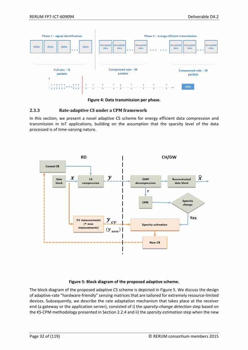
RERUM FP7-ICT-609094 Deliverable D4.2
Figure 4: Data transmission per phase.
2.3.3 Rate-adaptive CS under a CPM framework
In this section, we present a novel adaptive CS scheme for energy efficient data compression and transmission in IoT applications, building on the assumption that the sparsity level of the data processed is of time-varying nature.
Figure 5: Block diagram of the proposed adaptive scheme.
The block diagram of the proposed adaptive CS scheme is depicted in Figure 5. We discuss the design of adaptive-rate “hardware-friendly” sensing matrices that are tailored for extremely resource-limited devices. Subsequently, we describe the rate adaptation mechanism that takes place at the receiver end (a gateway or the application server), consisted of i) the sparsity-change detection step based on the KS-CPM methodology presented in Section 2.2.4 and ii) the sparsity estimation step when the new
Page 32 of (119) © RERUM consortium members 2015

Deliverable D4.2 RERUM FP7-ICT-609094
sparsity level along with the corresponding compression rate (that is fed back to the device) is estimated by utilizing a set of linear cross-validation (CV) measurements. The device/transmitter sends measurements to the receiver, which can identify a sparsity change and estimate the appropriate compression rate, which is communicated to the device through the feedback channel. The device further adapts the CS operation based on the feedback received.
2.3.4 CS compression and decompression
After the device collects a data block N∈x , we obtain the CS measurements curM∈y by
projecting x on the measurement matrix Φ . The number of measurements curM is chosen based
on the current compression rate NMCR curcur /1= − as it was determined by the receiver after the last sparsity-change detection. It is noted that at the initialization of the algorithm the device sends a compressed block at full rate ( 0=CR ) so that the receiver can make an accurate reconstruction and compute reliably the initial sparsity. Then, an appropriate compression rate based on computed sparsity is selected for the next block.
The received CS measurements are reconstructed at the receiver by using the OMP algorithm:
curKts ≤− 022 ..,minarg=ˆ
bΦΨbybb
(12)
where curK stands for the current sparsity level, as it was computed during the last sparsity estimation
step. The final estimate of the block is given by bΨx ˆ=ˆ .
Figure 6: Reconstruction error and OMP residual for light data.
To quantitatively assess the extend to which the reconstructed signal x can be sparsely represented
using curK elements of Ψ we propose to use the 2 norm of the residual error of OMP defined as
© RERUM consortium members 2015 Page 33 of (119)

RERUM FP7-ICT-609094 Deliverable D4.2
.ˆ= 2 xΦΨy −r (13)
We claim that the residual error r can be used as a metric of the reconstruction accuracy, based on the fact that according to the RIP imposed in the theory of CS, the low-dimensional projections y preserve with high-probability the distances in the original signal space. This idea is further supported by Figure 6, where the reconstruction error e of 500 consecutive blocks of compressively sampled light data from the Intel Berkeley Lab dataset5 is illustrated along with the corresponding value of r . All
blocks where compressed with 0.5=CR and reconstructed assuming 20=curK . It can be seen that
there is a clear resemblance in the pattern of reconstruction error e and OMP residual error r , motivating the use of the latter for detecting a sparsity change in the data collected by the device.
2.3.5 Measurement matrix design
In most CS systems the design of the measurement matrix Φ involves drawing each entry independently from a specific distribution (e.g. Gaussian, Bernoulli). Recently, a class of matrices, the so called structurally random matrices (SRMs), have been introduced [DGNT12] implementing the compression process in a structured three-step highly sparse process with nearly optimal performance in terms of the required number of measurements for accurate decompression.
Figure 7: Phase diagram for SRM.
Given a specific measurement matrix construction technique we can compute a phase diagram, namely a numerical representation of successful reconstruction probability over the space
2[0,1])/,/( ∈NMNK , as in [D10]. We discretize this space and perform multiple compression/decompression experiments at each grid point. The phase diagram is finally approximated by the percentage of trials that result in successful reconstruction, declared when
ethe ≤ , with eth an appropriately selected threshold. Afterwards, a logistic regression is fitted on
5 http://db.csail.mit.edu/labdata/labdata.html.
Page 34 of (119) © RERUM consortium members 2015

Deliverable D4.2 RERUM FP7-ICT-609094
the probability of correct reconstruction for each value of NK/ for creating a phase transition curve for a specific success probability. In Figure 7, the phase diagram for an SRM, constructed with a local pre-randomizer and Fast Walsh-Hadamard Transform (FWHT) of block size 16, is depicted along with 90% success phase transition curve.
We note that we construct the phase transition curve in an one-time, offline analysis. On computing the sparsity level, the receiver uses the phase transition curve as a lookup table to find the optimal measurement rate, or equivalently compression rate that feeds back to the device.
2.3.6 Sparsity change detection and estimation
After the reconstruction of the compressed block Φxy = at the receiver based on the current sparsity
level curK the new residual is fed as input to the KS-CPM algorithm that declares or not a change in sparsity level. In case of a sparsity-change alarm is raised, the receiver needs a mechanism for estimating the new sparsity level, thus an accurate decompression of the current block in terms of reconstruction error e .
Since we cannot calculate e explicitly, following the framework of [W09] we propose that the receiver
acquires an extra set of CS cross validation measurements xΦy cvcv = from the device, where cvΦ is a matrix whose entries are drawn from an i.i.d. Bernoulli distribution with zero mean and variance
r1/ . Then, for a given accuracy ε and confidence level ρ , we need ρ
ε21log2CM cv ≥ cross-
validation measurements for an estimate x in order to bound e as follows
.ˆ
)(11ˆ
))(1(131
2
22
2
22 PP
PPPP
PPcv
cvcv
cv
cvcv ey
xΦyy
xΦy −−
≤≤−
−+−
εεεε
(14)
with probability exceeding ρ−1 .
Subsequently, the device sends additional CS measurements to the receiver until the required error bound according to Equation (14) is satisfied. In order to avoid excessive computational burden due to a lot of reconstructions, the receiver performs decompression after every m additional measurements. In the current work, we fix 5=m . Finally, the sparsity of the accurately reconstructed signal is calculated and the appropriate number of measurements based on the phase transition curve technique described above is updated.
2.3.7 Theoretical evaluation
The performance evaluation of the proposed CS-based data gathering and transmission scheme was performed in both theoretical and experimental scenarios. The main metric used of the evaluation was the reconstruction error at the receiver, which clearly shows the impact of the scheme. The tests were done for (i) different measurement matrices, on order to show which category of matrices better fits the scheme, (ii) the adaptive scheme compared with a non-adaptive scheme to see what are the gains of the proposed adaptive scheme, and (iii) real experimental data.
2.3.7.1 Performance comparison of the CS-scheme against different measurement matrices
First, we evaluate the performance of the proposed CS-based scheme for two different types of matrices: the Gaussian and the Toeplitz. The performance is measured by means of reconstruction error ( e ) of synthetically generated signals. In particular, we generate blocks of 𝑁𝑁 = 100 samples with increasing sparsity levels 10% - 50%, i.e. 𝑘𝑘 = 10,20,30,40,50 non-zero DCT coefficients
© RERUM consortium members 2015 Page 35 of (119)

RERUM FP7-ICT-609094 Deliverable D4.2
independently drawn from a normal distribution 𝑁𝑁(0,1). We create 50 blocks for each sparsity level resulting in a total of 25000 samples. The first block of each sparsity level is used for the learning phase of the reconstruction error by the CH/GE where 100 independent trials of compression-decompression pairs are executed with compression rate that varies in [0.1,0.9]. The remaining 49 blocks are sent compressed based on the feedback received by the CH and are used for evaluation of the scheme.
Figure 8: Mean learned reconstruction error as a function of compression rate.
Figure 8 shows the learned reconstruction error trend (averaged over the 100 trials) against the compression rate for the Gaussian and a Toeplitz measurement matricesΦ , and for the sparsity levels 10%, 30% and 50%, respectively. As shown, the compressed signal can be accurately reconstructed up to a critical value of compression rate, for which the reconstruction error begins to increase. This critical value decreases with the sparsity level of the signal, clearly following the CS theory.
Regarding the performance of the two types of measurement matrices, it can be seen that sampling using a Gaussian measurement matrix generally leads in slightly lower reconstruction error. However, in the case of 30% sparsity, the signals sampled through a Toeplitz matrix are more accurately reconstructed in lower compression rates.
Having estimated the simulated reconstruction error per compression rate for a specific sparsity level, the GW evaluates the minimum number of measurements dictated by the QoS requirements. After incremented by a small safety fraction, which in the following is fixed in 5%, this number 𝑀𝑀𝑚𝑚𝑚𝑚𝑚𝑚 is sent back to the RD. Tables 1 and 2 present the mean reconstruction error averaged over the 49 per sparsity level evaluation blocks, for two different error thresholds, namely 𝑇𝑇ℎ𝑒𝑒𝑒𝑒1 = 0.1 and 𝑇𝑇ℎ𝑒𝑒𝑒𝑒2 = 0.01. From these results we make two basic observations. Firstly, our scheme is able to reach the QoS requirements for all sparsity levels and for both measurement matrices. Secondly, using a Gaussian
Page 36 of (119) © RERUM consortium members 2015

Deliverable D4.2 RERUM FP7-ICT-609094
matrix is clearly more efficient than a Toeplitz matrix by means of 𝑀𝑀𝑚𝑚𝑚𝑚𝑚𝑚 irrelevantly of sparsity level and reconstruction error threshold. This means that using a Gaussian matrix we can achieve the same reconstruction error using much less measurements, thus reducing significantly the transmission energy required by the devices to transmit the compressed signal.
Table 1: Mean reconstruction error for Ther1=0.1.
Sparsity level
Gaussian Toeplitz
minM Reconstruction error minM Reconstruction
error
10 % 37 0.0160 43 0.0597
20 % 53 0.0099 63 0.0365
30 % 69 0.0026 74 0.0171
40 % 79 0.0013 84 0.0092
50 % 90 0.0002 90 0.0005
Table 2: Mean reconstruction error for Ther2=0.01
Sparsity level
Gaussian Toeplitz
minM Reconstruction error minM Reconstruction
error
10 % 48 0.0114 310−× 53 0.0081
20 % 63 0.1675 310−× 74 0.0043
30 % 74 0.0331 310−× 85 0.0116 310−×
40 % 90 0.0005 310−× 90 0.0178 310−×
50 % 95 0.0004 310−× 95 0.0004 310−×
2.3.7.2 Performance comparison of the adaptive CS-scheme against a non-adaptive scheme
Here, we evaluate the proposed adaptive scheme in terms of reconstruction error “ e ” against a non-adaptive scheme that uses a fixed number of measurements to be transmitted and which cannot mitigate any changes in the signal sparsity. First, we show the performance on a synthetically generated dataset of signals with varying sparsity in the DCT domain. Then, we examine the behavior of the scheme on real data from an indoor sensor network deployment monitoring environmental variables (temperature, light illuminance). In both cases the data are compressed by using an SRM constructed through a local pre-randomizer and FWHT of block size 16.
A. Synthetic data
We generate blocks of 128=N samples with sparsity levels varying in 5%, 10%, 15% and non-zero DCT coefficients independently drawn from a normal distribution (0,1) . Each sparsity level is
© RERUM consortium members 2015 Page 37 of (119)

RERUM FP7-ICT-609094 Deliverable D4.2
chosen uniformly at random while the interval (in number of blocks) between two successive sparsity changes is also uniformly at random chosen in [50,200]. We change the sensitivity of the KS-CPM by varying the values of 𝐴𝐴𝐴𝐴𝐴𝐴0 in 100,200,500,1000 and repeat each experiment 50 times. We compare our scheme with a baseline non-adaptive strategy where all blocks are compressed using the mean compression rate of the corresponding adaptive scheme.
Figure 9: CDF of reconstruction error for synthetic data.
In Figure 9 the cumulative density function (CDF) of e is depicted for all different values of 𝐴𝐴𝐴𝐴𝐴𝐴0 and two different approaches. The solid curves correspond to the proposed adaptive scheme while the dashed lines correspond to the non-adaptive strategy. It is clear that the adaptive scheme substantially outperforms the non-adaptive one across all values of 𝐴𝐴𝐴𝐴𝐴𝐴0. It is further observed that the more sensitive the KS-CPM algorithm is, the less erratic the signal decompression is. This happens because of the decreased delay in the sparsity-change detection phase of the CPM that enables a fast adaptation of the compression rate. As a result, almost 95% of the blocks have a mean reconstruction error of 0.01 for 𝐴𝐴𝐴𝐴𝐴𝐴0 = 100.
B. Real experimental data
We further apply our scheme to real data from the Intel Berkeley Lab dataset6. In particular, we use light and temperature data captured once every 31 seconds form a subset of 20 sensors. We use 410 samples of each type (light and temperature) from each sensor that add up to a total of 5102× samples per type. As previously, we vary the sensitivity of KS-CPM in 100,200,500,1000 and repeat each experiment 50 times, choosing a different measurement matrix Φ each time.
6 http://db.csail.mit.edu/labdata/labdata.html
Page 38 of (119) © RERUM consortium members 2015
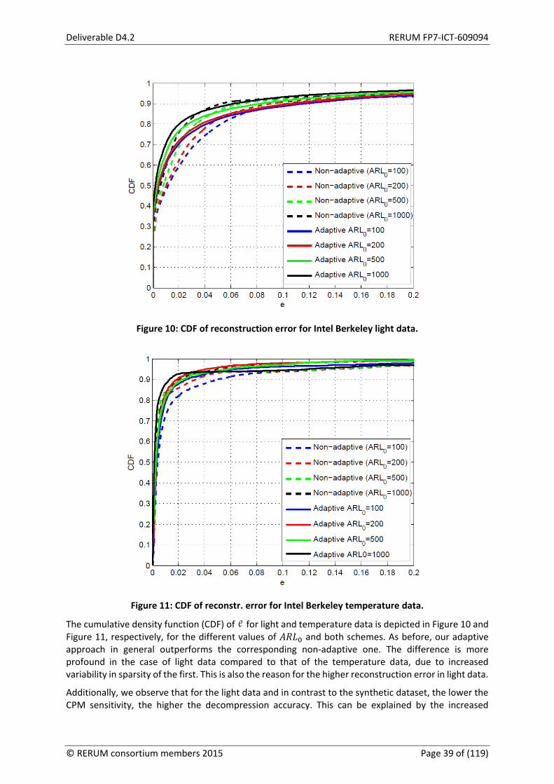
Deliverable D4.2 RERUM FP7-ICT-609094
Figure 10: CDF of reconstruction error for Intel Berkeley light data.
Figure 11: CDF of reconstr. error for Intel Berkeley temperature data.
The cumulative density function (CDF) of e for light and temperature data is depicted in Figure 10 and Figure 11, respectively, for the different values of 𝐴𝐴𝐴𝐴𝐴𝐴0 and both schemes. As before, our adaptive approach in general outperforms the corresponding non-adaptive one. The difference is more profound in the case of light data compared to that of the temperature data, due to increased variability in sparsity of the first. This is also the reason for the higher reconstruction error in light data.
Additionally, we observe that for the light data and in contrast to the synthetic dataset, the lower the CPM sensitivity, the higher the decompression accuracy. This can be explained by the increased
© RERUM consortium members 2015 Page 39 of (119)

RERUM FP7-ICT-609094 Deliverable D4.2
variability of the sparsity in the light data. If the CPM algorithm is highly sensitive a sparsity change is declared even for an abrupt and instantaneous variation in sparsity that can compromise the compression rate for several subsequent blocks. On the other hand, for a higher value of 𝐴𝐴𝐴𝐴𝐴𝐴0 the decreased sensitivity of the CPM prevents an unnecessary change is compression rate that will degrade performance. Thus, by using the adaptive scheme with 𝐴𝐴𝐴𝐴𝐴𝐴0 = 1000 almost 80% of the blocks has a reconstruction error lower than 0.02.
Similar observations can be also made for the case of temperature data, where, however, the adaptive scheme offers small performance improvement. In particular, we can see that by using the adaptive scheme with 𝐴𝐴𝐴𝐴𝐴𝐴0 = 1000 over 90% of the blocks has a reconstruction error lower than 0.01.
2.4 Data gathering using Compressive Sensing jointly with Matrix Completion
2.4.1 Background
IoT applications are mainly based on wireless infrastructures and often resource constrained devices like smart phones and sensor devices. Especially, when WSNs are used for information exchange between IoT devices, significant packet loss may arise. This is due to hardware limitations, buffer overflows, network protocol inefficiencies, etc. In this deliverable, we use the relatively new theory of matrix completion [CP10] for packet loss recovery by taking advantage of the often inter-spatial correlation between the collected data in a WSN.
Now, suppose there is a WSN consisting of n sensor devices that periodically sense the environment. After each measurement is taken, the related information is transmitted to a server called as sink. Based on the information transmitted by all sensors, the sink maintains a matrix where the measurements are stored. When packet loss occurs, this matrix has incomplete fields that correspond to the lost packets. MC allows us to recover this loss based on the remaining information that the sink has successfully received.
Suppose knM ×∈ is the unknown matrix we want to recover. As packet loss occurs in the network, the only information available about M is a set of entries jiM ×∈ , Ω∈),( ji , where Ω is the full set of entries kn× . At the sink, the available information can be summarized using )(MPΩ , where the sampling operator (due to packet loss) is defined by:
Ω∈
Ω otherwisejiifX
XP ijij 0,
),(,=)]([ (15)
We try to recover matrix M using information )(MPΩ . If knM ×∈ is a low rank matrix, one could recover it by solving
minimize rank(X)
subject to PΩ(Χ)=PΩ(M) (16)
as described in [CP10].
However, Equation (16) is both unstable and NP-hard, hence it cannot be easily used in practice. A widely used alternative is the convex relaxation:
minimize ‖𝑋𝑋‖∗
subject to PΩ(Χ)=PΩ(M) (17)
Page 40 of (119) © RERUM consortium members 2015
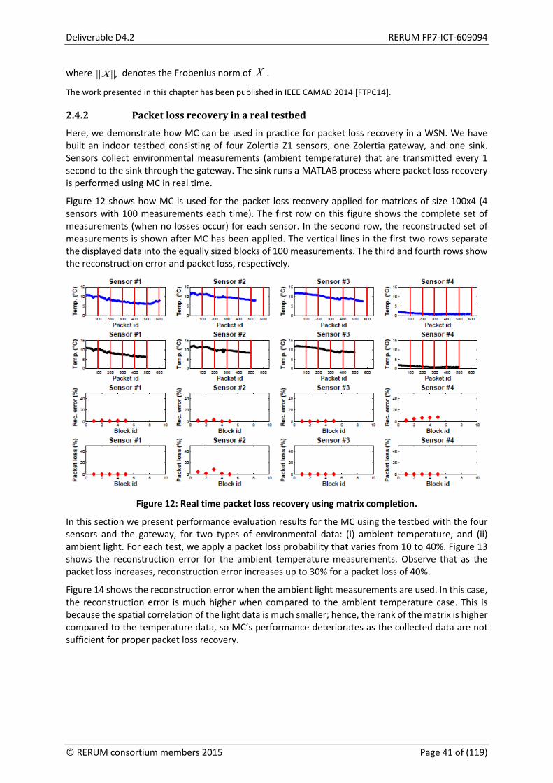
Deliverable D4.2 RERUM FP7-ICT-609094
where * X denotes the Frobenius norm of X .
The work presented in this chapter has been published in IEEE CAMAD 2014 [FTPC14].
2.4.2 Packet loss recovery in a real testbed
Here, we demonstrate how MC can be used in practice for packet loss recovery in a WSN. We have built an indoor testbed consisting of four Zolertia Z1 sensors, one Zolertia gateway, and one sink. Sensors collect environmental measurements (ambient temperature) that are transmitted every 1 second to the sink through the gateway. The sink runs a MATLAB process where packet loss recovery is performed using MC in real time.
Figure 12 shows how MC is used for the packet loss recovery applied for matrices of size 100x4 (4 sensors with 100 measurements each time). The first row on this figure shows the complete set of measurements (when no losses occur) for each sensor. In the second row, the reconstructed set of measurements is shown after MC has been applied. The vertical lines in the first two rows separate the displayed data into the equally sized blocks of 100 measurements. The third and fourth rows show the reconstruction error and packet loss, respectively.
Figure 12: Real time packet loss recovery using matrix completion.
In this section we present performance evaluation results for the MC using the testbed with the four sensors and the gateway, for two types of environmental data: (i) ambient temperature, and (ii) ambient light. For each test, we apply a packet loss probability that varies from 10 to 40%. Figure 13 shows the reconstruction error for the ambient temperature measurements. Observe that as the packet loss increases, reconstruction error increases up to 30% for a packet loss of 40%.
Figure 14 shows the reconstruction error when the ambient light measurements are used. In this case, the reconstruction error is much higher when compared to the ambient temperature case. This is because the spatial correlation of the light data is much smaller; hence, the rank of the matrix is higher compared to the temperature data, so MC’s performance deteriorates as the collected data are not sufficient for proper packet loss recovery.
© RERUM consortium members 2015 Page 41 of (119)

RERUM FP7-ICT-609094 Deliverable D4.2
Figure 13: Reconstruction error for the ambient temperature measurements for an increasing
packet loss.
Figure 14: Reconstruction error for the ambient light measurements for an increasing packet loss.
2.5 Compressive Sensing-based Routing The routing in WSNs is challenging due to the energy, transmission power, processing capacity and storage constrained nature of sensors. Furthermore, the global addressing and IP based routing in a large-scale WSN, as well as the significant redundancy of sensor data (often sensors record similar events) make routing a non-trivial task [AKK05]. In general, the choice of the optimum routing algorithm depends on a number of system architecture and design issues:
• Network mobility: mobile or stationary sensor nodes. • Node deployment: deterministic (sensors placed at known locations) or random (sensors
scattered randomly).
Page 42 of (119) © RERUM consortium members 2015

Deliverable D4.2 RERUM FP7-ICT-609094
• Multi-hop or single-hop considerations. • Energy considerations: multi-hop routing can consume less energy but introduces significant
overhead (e.g. delay). On the other hand, direct (single-hop) routing can perform well if the sensors and the sink are very close.
• Data delivery models: periodic-based, event-driven, query-driven, and hybrid. • Node capabilities: homogeneous or heterogeneous sensors in terms of processing capacity
and storage. For example, heterogeneous sensors may include more powerful sensors that can act as gateways.
• Data aggregation/fusion: data can be aggregated based on some statistical methods (e.g., for estimating values such as min, max, average, correlation, periodicities, and trends, or even for applying some advanced techniques, such as compressed sensing).
• Network topology/architecture (e.g., cluster based, ad-hoc vs. infrastructure/gateway/controller presence).
• Metrics for route selection. • Objectives (maximizing lifetime, maximizing throughput, minimizing delay, avoiding loops,
reliability, fault-tolerance, etc). The objectives of the related contributions found in the literature can be broadly classified into the following categories:
o Maximizing lifetime, where lifetime is defined as the worst-case time until a node becomes inoperable,
o Increase the performance in terms of several network-related parameters such as minimizing delay, maximizing throughput, etc.,
o Enhance the robustness of routing against path breakage and node mobility, o Delivery of real-time data.
2.5.1 Related work
Building on the fact that the readings of the sensors monitoring the same spatial region are highly correlated, the use of CS with routing schemes can reduce the number of the required sensor samples and the communication cost in WSNs. Assume a WSN consisting of N sensors where sensor readings of each time instant are generally represented by one dimensional vector N∈x that is assumed to be sparse in a basis N N×∈Ψ , such that =x Ψs , where N∈s is the corresponding sparse representation. The gathering and compression of x is realised though the linear process =y Φx . In the context of the CS-based routing M N∈ ×Φ represents the routing matrix, since each row corresponds to a routing path on which the packet sent is being mixed before arriving to the sink.
In the following, we use a simple example in order to demonstrate the CS-based routing principle in multi-hop WSNs. A WSN with four sensor nodes and one sink node is shown in Figure 1. If the projection vector is [ ]0.2,0.1,0.3,0.4i =φ then the projected value is
1 2 3 40.2 0.1 0.3 0.4i i x x x x= = + + +y φ x . The sink node can obtain this projected value by passing a message along the route S-1-2-4-3-S using source routing in the WSN.
The related work on CS-based routing contains a number of significant contributions. The authors in [QMM+09] consider joint routing and compressive sensing in a wireless sensor network. They use two types of signals: (i) synthetic signals using DCT and considering a frequency mask and a function transformation, and (ii) real signals like WiFi strength, ambient temperature, solar radiation, etc. For the real signals they consider four transformations: (i) discrete cosine transform (DCT), (ii) Haar wavelet (HV), (iii) Horz-diff (HD), and (iv) HorzVer-diff (HVF). Initially, they show that DCT and HV have a low sparsity degree, while HD and HVF have the highest (~=60, 70%). For the experiments they simulate a
© RERUM consortium members 2015 Page 43 of (119)
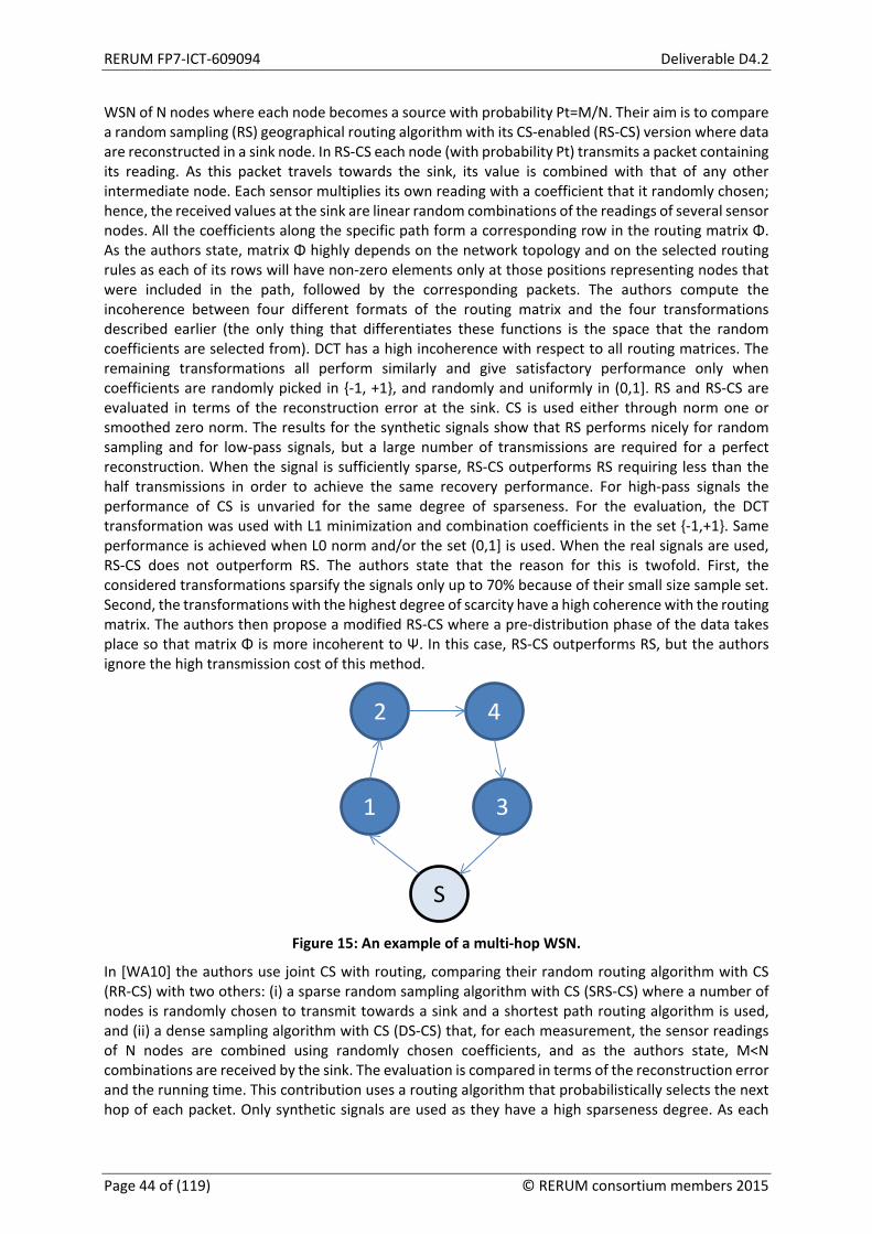
RERUM FP7-ICT-609094 Deliverable D4.2
WSN of N nodes where each node becomes a source with probability Pt=M/N. Their aim is to compare a random sampling (RS) geographical routing algorithm with its CS-enabled (RS-CS) version where data are reconstructed in a sink node. In RS-CS each node (with probability Pt) transmits a packet containing its reading. As this packet travels towards the sink, its value is combined with that of any other intermediate node. Each sensor multiplies its own reading with a coefficient that it randomly chosen; hence, the received values at the sink are linear random combinations of the readings of several sensor nodes. All the coefficients along the specific path form a corresponding row in the routing matrix Φ. As the authors state, matrix Φ highly depends on the network topology and on the selected routing rules as each of its rows will have non-zero elements only at those positions representing nodes that were included in the path, followed by the corresponding packets. The authors compute the incoherence between four different formats of the routing matrix and the four transformations described earlier (the only thing that differentiates these functions is the space that the random coefficients are selected from). DCT has a high incoherence with respect to all routing matrices. The remaining transformations all perform similarly and give satisfactory performance only when coefficients are randomly picked in -1, +1, and randomly and uniformly in (0,1]. RS and RS-CS are evaluated in terms of the reconstruction error at the sink. CS is used either through norm one or smoothed zero norm. The results for the synthetic signals show that RS performs nicely for random sampling and for low-pass signals, but a large number of transmissions are required for a perfect reconstruction. When the signal is sufficiently sparse, RS-CS outperforms RS requiring less than the half transmissions in order to achieve the same recovery performance. For high-pass signals the performance of CS is unvaried for the same degree of sparseness. For the evaluation, the DCT transformation was used with L1 minimization and combination coefficients in the set -1,+1. Same performance is achieved when L0 norm and/or the set (0,1] is used. When the real signals are used, RS-CS does not outperform RS. The authors state that the reason for this is twofold. First, the considered transformations sparsify the signals only up to 70% because of their small size sample set. Second, the transformations with the highest degree of scarcity have a high coherence with the routing matrix. The authors then propose a modified RS-CS where a pre-distribution phase of the data takes place so that matrix Φ is more incoherent to Ψ. In this case, RS-CS outperforms RS, but the authors ignore the high transmission cost of this method.
Figure 15: An example of a multi-hop WSN.
In [WA10] the authors use joint CS with routing, comparing their random routing algorithm with CS (RR-CS) with two others: (i) a sparse random sampling algorithm with CS (SRS-CS) where a number of nodes is randomly chosen to transmit towards a sink and a shortest path routing algorithm is used, and (ii) a dense sampling algorithm with CS (DS-CS) that, for each measurement, the sensor readings of N nodes are combined using randomly chosen coefficients, and as the authors state, M<N combinations are received by the sink. The evaluation is compared in terms of the reconstruction error and the running time. This contribution uses a routing algorithm that probabilistically selects the next hop of each packet. Only synthetic signals are used as they have a high sparseness degree. As each
2 4
1 3
S
Page 44 of (119) © RERUM consortium members 2015

Deliverable D4.2 RERUM FP7-ICT-609094
packet travels towards the sink, each intermediate node adds each measurement that has been multiplied with a random number in advance. However, the authors do not give any information regarding the selection of the random numbers. At the sink, the basis pursuit (BP) method is used for the reconstruction (this is a method for decomposing a signal into an “optimal” superposition of dictionary elements, where optimal means having the smallest L1 norm of coefficients among all such decompositions). The evaluation shows that the reconstruction error when RR-CS is used decreases as the number of the nodes that send data to the sink increases. Furthermore, RR-CS outperforms the other two algorithms in terms of the reconstruction error and the required running time (the authors assume that smaller running time leads to lower energy consumption).
The same concepts are used in [WA+10] where three CS-based routing algorithms are evaluated: (i) a weighted random routing algorithm (WRR-CS) where a node selection depends on its distance from the sink, (ii) a location-aware random routing algorithm (LRR-CS) where the network is divided into distinct parts and node selection is performed depending on node’s location in a specific part, and (iii) an annular routing algorithm (ARR-CS) where the network is divided into annular regions. For signal reconstruction (in the sink), the BP method is used. Algorithms’ evaluation is compared with SRS-CS and DS-CS, using synthetic signals in terms of the reconstruction error and the energy consumption. The results show that as the number of the sparsity level increases, the reconstruction error decreases. Furthermore, SRS-CS has the worst performance in terms of the reconstruction error, and then WRR-CS, ARR-CS and LRR-CS follow. DR-CS has the minimum reconstruction error. Regarding the energy consumption, DS-CS has the maximum (as expected) and then WRR-CS, LRR-CS, ARR-CS and SRS-CS follow.
In [LP++09] the authors study the performance of a joint routing and CS algorithm in terms of the achievable SNR at the sink and the energy cost. A randomly chosen node makes greedy choices for its next node on the path, by identifying another node within its communication range that will minimize the coherence of the transformation matrix with the (partially) updated routing matrix. Signals are reconstructed in the sink using the orthogonal matching pursuit algorithm. The proposed algorithm (LCPR) is compared to four other algorithms: (i) sparse random projection via shortest path, with opportunistic projection computations/compression (SRP), (ii) randomized down-sampling routed via shortest path (DS), (iii) projection augmented down-sampling via shortest path where nodes on the path contribute their data to the projection with some probability (ADS), and (iv) 2D wavelet based scheme shortest path routing. The signals are generated using two basis functions: (i) DCT, and (ii) multi-resolution 2D Haar basis. Furthermore, the signals are generated with three different levels of compressibility. The evaluation shows that when DCT is used, SRP’s performance is slightly better than the other schemes. For Haar, SRP outperforms the other schemes. Performance (SNR) increases as the number of the measurements increases. Regarding the SNR versus the energy ratio, LCRP, DS and ADS outperform SRP for both basis functions.
The paper in [LPS+09] uses joint routing and CS, considering two clustering approaches: (i) square clustering, and (ii) shortest-path tree clustering (SPT). Furthermore, two types of reconstruction are used: (i) independent, and (ii) joint. The signals are generated using DCT and Haar. Reconstruction is performed using the gradient pursuit for sparse reconstruction method. Performance evaluation is performed in terms of the SNR and the cost. The simulation results show that joint reconstruction outperforms independent reconstruction (square clustering and Haar were used). Furthermore, the performance (SNR versus cost ratio) of the SPT is higher than that of the square clustering, for different number of clusters.
Finally, in [LLQ10] the authors propose an algorithm working as follows: initially, a few projections are performed (using Bayesian compressed sensing-BCS) assisting the sink node to determine a node i that has the least coefficient power (LCP). LCP is a metric that indicates the strength of the contribution of a node’s data to the projections. Then, from node i to sink, a greedy algorithm is used to find two paths that maximize the so-called differential entropy. A new projection is produced and reconstruction takes place. Evaluation is performed in terms of the reconstruction error, communication cost, and
© RERUM consortium members 2015 Page 45 of (119)

RERUM FP7-ICT-609094 Deliverable D4.2
computation complexity. The proposed algorithm is compared to: (i) BCS, (ii) adaptive BCS, and (iii) adaptive CS. The results show that the proposed algorithm has nearly the same good performance (in terms of the reconstruction error) as the BCS. Adaptive BS has the worst performance. Regarding the communication cost: it is fixed for BCS and adaptive BCS, while the cost for the adaptive algorithms varies for different experiments. Adaptive CS has the least communication cost, while the proposed algorithm consumes about 2% more. The proposed algorithm consumes less CPU time than the adaptive CS but more than the adaptive BCS.
2.5.2 Joint CS and routing
In this section we describe how CS-based routing can be used in a WSN, and the performance of two heuristic algorithms: (i) a shortest path with largest information gain per energy, and (ii) a greedy path. We assume a WSN modelled as a graph ( ),G V E= where V is a set of N sensor nodes and E is the
set of edges between nodes that are within the communication range of each other. The sensors are assumed to be synchronized. Each time t the readings of the sensors form a snapshot of the measured
field denoted as [ ]1,...,T
Nx x=x . Additionally, we assume that the energy consumed for sensing and
computation is negligible, as energy consumption is dominated by the radio communications. In the following, energy consumption will be estimated using the total number of transmissions necessary to collect the information of the data field.
Assume a signal Ν×Ν∈x that is K -sparse in a given basis Ν×Ν∈Ψ , such that =x Ψs , 1N×∈s with
0K=s and K N . According to CS acquisition model, we can acquire x from a set of
( )logM O K N= ( M N< ) projections ( )= +y Φ x ε , where Μ×Ν∈Φ is the measurement matrix
and 1N×∈ε is the sensor noise. If Φ is incoherent to basis Ψ we can reconstruct x by solving the following regularized 1 optimization problem:
2
2 1ˆ arg min ρ= − +
ss y ΦΨs s , (18)
where the scalar ρ controls the relative importance applied to the Euclidian error and the sparseness. Then, the original signal is restored as ˆˆ =x Ψs . CS performance is evaluated using the
normalized reconstruction error defined as 2
2
ˆe
−=
x xx
. Error e essentially expresses how much
signals x and x differ. The smaller e is, the higher the fidelity of x to x , therefore, the higher CS performance is.
A large number of algorithms have been proposed to solve Equation (26) including convex relaxation, linear programming and greedy approaches. However, most of these algorithms can only compute a point solution s providing no sense of confidence in the estimated elements of s . Bayesian compressive sensing (BCS) [SYC08] provides an efficient way to solve this problem by providing a full posterior density function of s and, thus, a posterior density function of x . In particular, if μ and Σ are the mean and covariance matrix of posterior density function of s , as calculated by the BCS algorithm, then the posterior density function of x is Gaussian with mean and covariance:
( )( )
E
Cov Τ
=
=
x Ψμ
x Ψ ΣΨ (19)
Most of the compressive sensing algorithms proposed are non-adaptive which means that projection vectors are not chosen according to information collected so far. However, BCS algorithm providing
Page 46 of (119) © RERUM consortium members 2015

Deliverable D4.2 RERUM FP7-ICT-609094
point estimation of reconstructed signal along with associated error bars can be leveraged to adapt projections and reduce uncertainty in the estimation of x . In order to maximize reduction in uncertainty of estimation (as expressed by the differential entropy reduction H∆ the new projection vector 1M +r is calculated as the solution to the following maximization problem:
( )1 arg max TM + =
rr r Σr (20)
CS uses projections to gather information. For a snapshot of the noisy data field noisy = +x x ε , a
projection on the projection vector [ ]1,...,T
Nr r=r is defined as 1
NT noisy noisy
i ii
r x=
=∑r x . The sink can
obtain this projected value without the sensors sending their readings directly to the sink. Instead, a message passes along the nodes corresponding to the non-zero elements of projection vector (which practically defines a routing path). As the message travels through the path, each sensor computes its contribution to the projected value and adds it to the intermediate result. Then the sensor writes the new intermediate value to the message and forwards the message to the next hop, until sink is reached.
Although Equation (28) provides an optimal projection in terms of differential entropy reduction, this solution is usually dense and the energy required to acquire a projection is not taken into consideration. The energy required to acquire a projection depends on the length of the tour to obtain the projection, in other words, on the locations of the non-zero coefficients in the projection vector. As a result, the choice of the coefficients of a projection vector should consider both information content and energy expenses.
Following the analysis in [CRH09] we describe the derivation of the expected information gain of a projection vector. We assume that we have already measured k projections over the data field denoted as:
( ) ( )k k k= + = +y Φ x ε Φ Ψs ε (21)
As a first step we de-correlate the noise in the projected values, since a noisy sensor reading can appear in multiple projections. For this reason, we compute the Cholesky factorization of T T=ΦΦ R R and multiply from left Equation (21) with T−R to obtain the new equation:
T T Tk k k
− − −= +R y R Φ Ψs R Φ ε (22)
By inputting Tk k
−=y R y and Tk k
−=Φ R Φ Ψ to BCS algorithm we get an estimate of unknown
vector, s , and estimated unknown noise variance, 2σ , along with an estimate of the posterior density distribution of data field x , which is Gaussian distributed with mean Ψμ and covariance TΨ ΣΨ . Then, the reduction in differential entropy H∆ in the estimate of the unknown data field by using an additional projection vector 1
1 1: 0N Tk k
×+ +∈ ≠r V r , with 1 2
1k+ =r is given by:
( ) 1 11 2
1 1
1 1log 1ˆ2
T T T Tk k
k T Tk k
Hσ
+ ++
+ +
∆ = +
r VV ΨΣΨ VV rrr VV r
, (23)
where V is the orthonormal basis of the null space of Φ .
© RERUM consortium members 2015 Page 47 of (119)

RERUM FP7-ICT-609094 Deliverable D4.2
In order to achieve a balance between information gain and energy consumption in the i-th iteration the projection vector r is chosen to maximize the ratio:
( ) ( )( )
HQ
E∆
=r
rr
, (24)
where ( )E r is the minimum energy (in terms of number of transmissions) needed to acquire the
projection ( )T +r x ε at the sink. Maximization of ( )Q r is proved to be NP-hard, so two heuristics are
used in order to determine good projection vectors, which is equivalent to finding (i) the locations of non-zero coefficients of the projection vector and (ii) the values of non-zero coefficients.
2.5.2.1 Heuristic algorithms
2.5.2.1.1 Shortest path (Heuristic Algorithm 1)
Assume a sensor node i V∈ and let iP denote the set of sensor nodes along the shortest path from i
to the sink, excluding sink. Abusing the notation we can write iP∈r if non-zero elements of r
correspond to only to sensors in iP . Then, the optimal projection is:
( )1,...,
maxarg max
2iP
opt i Ni
HP
∈
∈
∆= r r
r (25)
Although simple and straightforward, this path calculation doesn’t take into consideration entropy reduction.
2.5.2.1.2 Greedy path (Heuristic Algorithm 2)
In attempting to find a path with good ratio of entropy reduction to path length this algorithm iterates N times, beginning each time from node i V∈ . In each iteration, a path iP from node i to the sink is
greedily determined. Specifically, if node j is the last selected node included in iP , node j+1 will be the closer-to-the-sink neighbour of node j that maximally reduces differential entropy of the so far determined projection. Finally, the optimal projection in given again by Equation (25), where iP are now the greedily created paths.
2.5.2.2 Performance evaluation
In order to evaluate the performance of the heuristic algorithms presented we consider a WSN of 54 nodes randomly deployed in square cells formed by a grid on a square area with side 200m. Each node can have up to 8 neighbours, while the sink is located at the centre of the area. We assume that a shortest path tree has already been built in the network. An example of network topology along with the corresponding shortest path tree is depicted in Figure 16. We use 2000 snapshots of temperature and humidity sensor readings, provided by a deployment of 54 Mica2Dot sensors at Intel Berkeley lab employed with weather boards. We use DCT as the sparsifying basisΨ , as it is able to express sparsely smooth signals, like temperature and humidity. We assume that initially 13 random sensors return their readings to the sink and then 41 more adaptive projections are performed, using the heuristics presented.
We measure the performance based both on accuracy and energy consumption. As regards accuracy, normalized reconstruction error e is used, while for energy consumption we count the total number of transmissions used in up to each adaptive projection. Let T represent the number of transmissions
Page 48 of (119) © RERUM consortium members 2015

Deliverable D4.2 RERUM FP7-ICT-609094
then we express the results with relative energy consumption / refJ J , where refJ is the total number
of transmissions if all sensors send their data to the sink.
Figure 16: Example of network topology.
Figure 17 and Figure 18 depict the performance of the two heuristic algorithms for the temperature data and the humidity data, respectively. The results are averaged over all 2000 snapshots. Obviously, Heuristic algorithm 2 outperforms Heuristic algorithm 1 for both cases, since it is able to achieve lower reconstruction error for the same energy consumption. For example, in case relative energy consumption is 0.7, we can achieve 5%-6% reduction in reconstruction error, for both signal types. This is normal because Heuristic algorithm 2 makes use of a better chosen path in order to balance accuracy and energy consumption.
Figure 17: Performance of heuristic algorithms for temperature data.
2.5.3 Conclusion
In this chapter we described how CS can be used in order to minimise the sampling and transmission costs within a WSN. We proposed an adaptive CS scheme where the compression rate used for CS is decided by a central node (sink) based on the required QoS. We proposed to use structurally random matrices in order to compress efficiently the captured data at device and associate sparsity estimates to minimum compression rate through a pre-computed phase transition curve as a lookup table. A possible sparsity change is detected at the receiver by applying a CPM algorithm. The sparsity estimation mechanism involves the collection side information in the form of extra cross-validation
0.3 0.4 0.5 0.6 0.7 0.8 0.90.055
0.06
0.065
0.07
0.075
0.08
0.085
0.09
0.095
relative energy consumption J/Jref
Nor
mal
ized
rec.
erro
r e
Heuristic algorithm 1Heuristic algorithm 2
© RERUM consortium members 2015 Page 49 of (119)

RERUM FP7-ICT-609094 Deliverable D4.2
measurements. The updated minimum compression rate is sent from the receiver to the device through a feedback mechanism. Our results show that the proposed mechanism improves performance of non-adaptive CS both on synthetic and real experimental data.
Figure 18: Performance of heuristic algorithms for humidity data.
As it is well known, severe packet loss can occur in a WSN because of the interference, protocol inefficiencies and other reasons. We demonstrated how CS combined with MC can recover the missing information due to packet loss. The evaluation results show that CS jointly with MC, give a small reconstruction error for fairly high compression ratios, and for a significant packet loss. Missing information is sufficiently recovered, and the total energy consumption of the sensors substantially reduces.
Finally, we demonstrated how CS can be jointly used with routing for energy efficiency. We evaluated two heuristic algorithms using ambient temperature and humidity data, in terms of the reconstruction error. The heuristic algorithm that chooses routing paths in a greedy fashion achieves a lower reconstruction error, as it balances energy consumption more efficiently among the routing paths.
0.3 0.4 0.5 0.6 0.7 0.8 0.90.045
0.05
0.055
0.06
0.065
0.07
0.075
0.08
0.085
0.09
relative energy consumption J/Jref
norm
aliz
ed re
c. e
rror e
Heuristic algorithm 1Heuristic algorithm 2
Page 50 of (119) © RERUM consortium members 2015

Deliverable D4.2 RERUM FP7-ICT-609094
3 Sleep and Wakeup Techniques for Energy Saving This entire section focuses on techniques that reduce overall device energy consumption by regularly putting RDs and Gateways to sleep mode, while at the same time still enabling end-to-end communications in a reliable manner. For RDs in particular, radio operation and especially idle radio listening is a major factor of energy drain and therefore should be kept to a minimum.
The first technique discussed here (Section 3.1) focuses on duty-cycled radio operation with congestion awareness. By reducing congestion on a low-power wireless network we decrease packet re-transmissions and also we reduce the amount of time a node has to spend awake before it can exit its congested state. Congestion is likely to occur on event-based deployments, whereby changes to an observable parameter (e.g. ambient temperature) can lead to multiple devices attempting to transmit data simultaneously.
The second technique (Section 3.2) focuses on energy-aware relay properties of gateways. The contributions of this work offer insights into the possible performance gains by randomly activating or deactivating Full- or Half-Duplex gateway nodes and the impact of the number of RD and gateways that are served by such network configurations.
Those two improvements ultimately lead to the reduction of energy consumption on a per-node basis as well as network-wide.
3.1 Congestion Aware Duty Cycling RDs in 6LoWPANs Sensor deployments aim for many years of isolated operation with no servicing to change energy sources. This is of immediate relevance to RERUM’s UC-O2: Environmental Monitoring. Energy consumption is therefore a significant consideration. Idle radio listening is a major energy consumer [MGOP12] and to prolong the lifetime of a sensor deployment many efforts have been made in the development of Radio Duty Cycling (RDC) algorithms. With these RDCs, nodes keep their receivers off in order to minimise idle listening energy consumption. On the other hand, RDCs typically have a negative impact on network resource utilisation (e.g. bandwidth) and significantly increase congestion [MGOP11]. An RDC algorithm that uses a fixed sleep/wake-up cycle period is henceforth called a “Fixed RDC”, whereas an RDC algorithm that allows period adaptation is called “dynamic”. CADC [MOPG14] is a congestion-aware, dynamic duty cycling mechanism tailor-made for 6LoWPANs [MKHC07].
The work discussed in this sub-section is joint work with Loughborough University, Computer Science and has been published in [MOPG14].
3.1.1 Motivation and relation to use cases
In scenarios involving event-based deployments, network traffic is of a very bursty nature: The network is idle for most of the time with the only traffic being occasional network control packets. When an event occurs to a parameter under observation, multiple RDs may attempt to transmit simultaneously. An example of this is the simultaneous transmission of ambient temperature readings when the measured temperature exceeds a high threshold. Congestion leads to packet losses, which in turn lead to re-transmissions thus causing energy consumption that could have been avoided by proactively preventing the network congestion. Furthermore, while the network is in a congested state, RDs will stay awake for a period of time in order to resolve it, and this leads to additional energy consumption.
The scheme proposed here is relevant to UC-O2 - Environmental monitoring, whereby deployments will be formed by a large number of devices. Topologies are potentially going to be very dense and this makes them particularly susceptible to congestion due to a large number of devices occupying the wireless medium in the small geographic area. In cases of battery-powered RDs, it is impractical or outright untenable to replace batteries very frequently due to high management cost and possibly hard-to-reach installation locations. Thus, long battery life is important and the proposed scheme perfectly fits the requirement for prolonging the network lifetime. For devices powered from mains,
© RERUM consortium members 2015 Page 51 of (119)

RERUM FP7-ICT-609094 Deliverable D4.2
low energy consumption is also important in order to reduce financial cost, but also in order to comply with national and international regulations where applicable.
For the indoor use cases, the devices can be plugged in the power outlets, so energy efficiency may not be so critical. However, frequent battery replacement is a costly nuisance for the end user, while regulations also need to be adhered to.
The scheme is not relevant to the smart transportation use-case.
3.1.2 A brief introduction to Radio Duty Cycling with Contiki
The Radio Duty Cycling (RDC) layer sits in the Contki network stack between the Medium Access Control (MAC) layer and radio drivers. The MAC layer handles Carrier Sense Medium Access (CSMA) and retransmissions with exponential backoff when applicable. The RDC layer’s purpose is to turn the radio on/off (duty-cycle) in order to reduce energy consumption, while at the same time maintaining network connectivity. Contiki offers two choices for the RDC layer: ContikiMAC [D11] and NullRDC, the latter not really being a duty-cycling algorithm since it simply keeps the radio always on.
With ContikiMAC, a node wakes up every few milliseconds and checks the channel for traffic. This interval is called Channel Check Interval (CCI) or Channel Sampling Period. If no traffic is present, the radio transceiver is turned back off. If traffic is detected, the node stays on until complete reception. To send a frame, a node will transmit it repeatedly (strobes) for slightly longer than CCI, waiting for a brief time interval between two strobes for a potential acknowledgement frame (ACK). This repeated transmission, often called a “packet train”, lasts long enough for intended recipients to wake up, detect the packet and receive it, irrespective of exactly when they last went to sleep. This removes the complexity of maintaining synchronisation between neighbours. In the case of unicast packets, the receiver will send an ACK frame, causing the sender to terminate its chain of strobes and thus conserve energy. However, broadcast frames must be received by all neighbours and there are no ACKs; the sender always has to go through the entire packet train, as illustrated in Figure 19. Thus, broadcast transmissions are fundamentally more costly. The actual implementation of the ContikiMAC algorithm is more sophisticated and optimised by supporting features such as phase locks and support for burst traffic, but the concept remains the same.
Figure 19: Broadcast frame transmission with ContikiMAC (Source [OPT13]).
Page 52 of (119) © RERUM consortium members 2015

Deliverable D4.2 RERUM FP7-ICT-609094
3.1.3 Related work on Radio Duty Cycling for Wireless Sensor Networks
S-MAC [YHE02] is an early and pioneering RDC MAC for sensor networks. With this mechanism, nodes must have their clocks synchronised. In order to address the low bandwidth and latency issues, S-MAC can transmit multiple packets in a single transaction. T-MAC [DL03] improves upon S-MAC by implementing new techniques such as future- RTS. These techniques reduced latency but are limited to 3-hops distance from the originator. X-MAC [BYAH06] attempts to minimise the active listening time by transmitting short preambles with the destination address. Receiver nodes will check if the preamble’s destination address belongs to them. If it does, and acknowledgement is send and the receiver waits for the data packet. In ContikiMAC [D11], nodes wake up every few milliseconds and check the channel for traffic, as described in detail in Section 3.1.2.
Fixed RDC MACs must be tuned to a specific achievable throughput and thus there is a need to manage the trade-off between energy use and throughput. This in turn may lead in low bandwidth configurations with high percentage of packet losses or very high energy usage [D11].
A number of dynamic RDC MAC protocols have been proposed to balance the trade-off between energy use and available throughput. In TA-MAC [CYL08], all nodes must be synchronised. This is achieved through the transmission of frequent, broadcast SYNC packets. In TA-MAC the RDC is not altered under any network conditions; instead under heavy network load, two or more packets may be transmitted in a single cycle. In DCLA [PP10], one node will operate as the coordinator and assigns the wake up frequency to the rest of the network based on the traffic requirements. To achieve this, the coordinator gathers information embedded in the MAC header of the frame by the end-devices. When a coordinator node has no gathered information, wake up frequency is calculated by the DCLA agent using a technique known as Q-Learning. BEAM [AWBD10] is designed as an improvement upon X-MAC. BEAM comprises two operational (basic and short- preamble) modes in order to optimise receiver sleep time. In basic mode, transmitted preambles include the payload. Therefore, receiver nodes receive and acknowledge the data upon the reception of the preamble. In short-preamble mode, preambles do not include any payload. Therefore, transmitter nodes will not send any data before the acknowledgement of the preamble. BEAM switches between the two modes based on the packets payload (basic mode > 40 bytes). In ADCC [BY13] a method that controls the duty cycle through queue management is proposed. A feedback controller is used in order to determine a node’s sleep time based on the local information. Additionally, a synchronisation scheme using an active pattern is put in place. It represents the active time slot schedule for synchronisation among sensor nodes, without affecting neighbouring schedules.
Many dynamic RDC schemes have been proposed and designed for IEEE 802.11 networks. It has been demonstrated that an IEEE 802.11b network cannot capture the RDC aspects of modern WSNs, nor the low-power, lossy nature of IEEE 802.15.4-compliant radio hardware [CH10].
3.1.4 CADC implementation
CADC is designed as an extension to ContikiMAC aiming to provide an improvement in the areas where traffic patterns vary, such as when supporting multiple applications on a single WSN. ContikiMAC is based on periodic Channel Checks and can achieve up to 99 % sleep durations [D11]. Additionally, high wake up frequency configurations can achieve very high goodput and low delay on the cost of energy. Combining the above observations with the various, multiple and unpredictable traffic patterns generated in 6LoWPANs, configuring a deployment with the appropriate RDC can prove to be a challenging task. Therefore, a dynamic RDC protocol for 6LoWPAN sensor networks should be tailored to the “low-power and lossy” requirements of IEEE 802.15.4 and be Topology independent and capable of incorporating of multiple sinks. It should also support for bidirectional traffic with varying traffic load. Fundamentally it should be capable of local decision making in adjusting the Channel Check Rate (CCR) rather than reconfiguring the whole network. For the remainder of this deliverable, RDC in WSN will be expressed through the CCR: 𝐶𝐶𝐶𝐶𝐴𝐴 = 1/𝑃𝑃, where P is the period of the duty cycle in seconds.
© RERUM consortium members 2015 Page 53 of (119)

RERUM FP7-ICT-609094 Deliverable D4.2
3.1.4.1 General characteristics and rules
In order to achieve fast adaptation, CADC operates as follows: Every N packet transmissions each node measures its congestion levels. If a node has no inbound traffic at the MAC layer within a period of time P, it is considered idle. Idle nodes reset their CCR to the default value. P is related to the node’s CCR, with higher CCRs corresponding to smaller periods, as nodes can transmit a greater number of packets per second and thus the probability of congestion increases.
Every CADC node follows these rules:
• A CADC node must always have the same or lower CCR than its parent nodes (for bi-directional traffic, a node must have the same CCR as its parent and children).
• Information about a node’s CCR must frequently be forwarded to parents (the receivers of the node’s traffic).
• When a node becomes idle, its CCR will return to the default configuration, the minimum CCR.
CADC’s operation transitions among 5 possible states based on a node’s measured congestion levels.
3.1.4.2 Congestion levels and rate adaptation
Queue occupancy is considered a sufficient method for congestion detection when traffic patterns are many-to-one, which is the predominant case for 6LoWPANs. However, in cases with arbitrary communication traffic patterns and varying duty cycles this may be insufficient. Nodes require a higher degree of knowledge in order to adjust their duty cycles efficiently. Every N transmissions CADC measures 5 parameters and calculates the optimal CCR:
i. Packet-queue occupancy. CADC uses two queue thresholds 𝑄𝑄ℎ and 𝑄𝑄𝑙𝑙 in order to estimate the probability of a packet loss due to queue-overflow (𝐴𝐴 ≈ 𝑄𝑄ℎ: high probability, while 𝐴𝐴 ≈ 𝑄𝑄𝑙𝑙: low probability, with 𝐴𝐴 being the current queue length).
ii. Ratio of successful transmissions to the failed transmission threshold:
𝐴𝐴𝑠𝑠𝑠𝑠𝑠𝑠𝑠𝑠 =𝑇𝑇𝑠𝑠𝑠𝑠𝑠𝑠𝑠𝑠
𝐹𝐹𝑡𝑡 (26)
where 𝑇𝑇𝑠𝑠𝑠𝑠𝑠𝑠𝑠𝑠 is the number of successfully transmitted packets and 𝐹𝐹𝑡𝑡 is a transmission threshold for non acknowledged packets (collisions and other losses are not calculated in this).
iii. Ratio of failed transmissions to transmission threshold:
𝐴𝐴𝑓𝑓𝑓𝑓𝑚𝑚𝑓𝑓 =𝑇𝑇𝑓𝑓𝑓𝑓𝑚𝑚𝑓𝑓
𝐹𝐹𝑡𝑡 (27)
where 𝑇𝑇𝑓𝑓𝑓𝑓𝑚𝑚𝑓𝑓 is the number of transmissions failed due to un acknowledged packets. If 𝐴𝐴𝑓𝑓𝑓𝑓𝑚𝑚𝑓𝑓 > 1 it is highly possible that there is a CCR misconfiguration between a child and a parent node. This can also be due to a bad link, but this is handled by the routing protocol and cannot be addressed at the MAC layer.
iv. Ratio of successful transmissions to the sum failed transmissions and incoming traffic:
𝐴𝐴𝑠𝑠𝑒𝑒𝑒𝑒𝑠𝑠𝑚𝑚𝑠𝑠𝑒𝑒 =𝑇𝑇𝑠𝑠𝑠𝑠𝑠𝑠𝑠𝑠
𝑇𝑇𝑓𝑓𝑓𝑓𝑚𝑚𝑓𝑓 + 𝐼𝐼𝑁𝑁𝑡𝑡 (28)
Page 54 of (119) © RERUM consortium members 2015

Deliverable D4.2 RERUM FP7-ICT-609094
where 𝐼𝐼𝑁𝑁𝑡𝑡 is the incoming traffic at the MAC layer. When 𝐴𝐴𝑠𝑠𝑒𝑒𝑒𝑒𝑠𝑠𝑚𝑚𝑠𝑠𝑒𝑒 > 1 packet queues are draining. If 𝑇𝑇𝑓𝑓𝑓𝑓𝑚𝑚𝑓𝑓 = 0, 𝐴𝐴𝑅𝑅𝑅𝑅𝑟𝑟𝑣𝑣𝑣𝑣𝑣𝑣𝑅𝑅 is considered > 1.
v. The highest CCR announced by a node’s children (CCRannounced).
CADC changes its state based on the above values. Figure 20 shows a detailed state transition diagram while their detailed description follows:
• Congestion collapse: A node is or it is about to become heavily congested. A node will enter this state if its packet queue levels are above the high threshold 𝑄𝑄ℎ, 𝐴𝐴 𝑠𝑠𝑠𝑠𝑠𝑠𝑠𝑠 < 1 and its current 𝐶𝐶𝐶𝐶𝐴𝐴 < 𝑚𝑚𝑓𝑓𝑚𝑚𝐶𝐶𝐶𝐶𝐶𝐶
4. This indicates that there is a high probability for packets loss and thus CCR
must be rapidly increased. • Congested: A node is lightly congested. A node will enter this state if its packet queue level is
above the lower threshold 𝑄𝑄𝑓𝑓, 𝐴𝐴 𝑠𝑠𝑒𝑒𝑒𝑒𝑠𝑠𝑚𝑚𝑠𝑠𝑒𝑒 ≤ 1, and it entered the congestion collapse state, but its CCR increase cannot fulfill congestion collapse requirements.
• Over duty cycle: A node is operating with a higher CCR than necessary. A node will enter this state when packet queue level is below the lower threshold 𝑄𝑄𝑓𝑓, the CCR in the node is higher than CCRannounced (rule i), 𝐴𝐴𝑠𝑠𝑒𝑒𝑒𝑒𝑠𝑠𝑚𝑚𝑠𝑠𝑒𝑒 ≤ 1 and 𝐴𝐴𝑓𝑓𝑓𝑓𝑚𝑚𝑓𝑓 < 1 and the node’s CCR is higher than 𝑚𝑚𝑣𝑣𝑚𝑚𝐶𝐶𝐶𝐶𝐶𝐶. When a node successfully enters this state, its CCR will be halved.
• Normal operation: The default state (no congestion), nodes will maintain their current CCR. • Forwarding: This is an intermediate state for the purpose of informing receiver nodes about
imminent CCR changes. Before a CCR increase, a node will enter the forwarding state and remain there for a Guard Period related to the min CCR. In this state, the duration of packet transmissions is related to 𝑚𝑚𝑣𝑣𝑚𝑚𝐶𝐶𝐶𝐶𝐶𝐶 and thus it is ensured that CCR adaptation information is propagated to the appropriate nodes. When this period is over, the node switches to the new CCR.
3.1.4.3 Information sharing among nodes
In order to achieve optimal network performance, nodes share their CCR as it changes with their parent nodes using the 3 reserved bits of the Frame Control Field (FCF) in the 802.15.4 frame header. If the sender’s CCR frame is higher than the receiver’s current rate, nodes will adjust their CCR and send the new value (Figure 21).
3.1.4.4 Frame retransmission scheme
In a 6LoWPAN, tasks such as neighbour discovery and routing use a combination of layer 3 unicast and link-local multicast datagrams. At layer 2, these get transmitted as unicast and broadcast frames respectively. ContikiMAC repeatedly transmits a frame for a period of time related to its CCR, with parameters set so the node is guaranteed to wake up during the packet train. When nodes operate with different CCRs, broadcast frames are rendered unreliable since both packet train durations and node sleep times will be different between the nodes. In order to prevent this, CADC sets the duration of broadcast packet trains to a fixed value regardless of CCR. This modification can in turn cause continuous collisions to nodes with a high CCR as the duration of unicast packet-trains will be much shorter. CADC confronts this by improving the traditional CSMA back-off algorithm through the application of multiple packet retransmission windows for the different cases of collisions. When a collision is caused by a unicast frame, the back-off time will be based on the node’s current CCR. When collisions are caused by broadcasts, the back-off time will be based on the fixed duration related to 𝑚𝑚𝑣𝑣𝑚𝑚𝐶𝐶𝐶𝐶𝐶𝐶.
© RERUM consortium members 2015 Page 55 of (119)

RERUM FP7-ICT-609094 Deliverable D4.2
Figure 20: CADC state transition diagram.
Figure 21: CADC traffic flow scenarios.
Page 56 of (119) © RERUM consortium members 2015

Deliverable D4.2 RERUM FP7-ICT-609094
3.1.5 Evaluation of CADC’s energy consumption
For our evaluation we use Cooja [O06], the wireless network simulator distributed with the Contiki OS. It allows the emulation of real hardware platforms in a simulated IEEE 802.15.4 wireless network. ContikiMAC serves as a base line for our comparisons. Additionally, we compare with X-MAC because of its popularity and with BEAM as its dynamic RDC approach makes it very relevant to this work. For our tests we use CBR traffic with a 24 byte application-layer payload 1-8 hops distance between the source and the destination. Outgoing MAC-layer packet queues were set to 10 packets. In Contiki, the default configuration of CCR is 8. We conducted comparisons with multiple different static CCR configurations to get more representative results.
The packet transmission intervals used during the simulations were: 500 ms, 250 ms, 125 ms and 62.5 ms. This range of CCR values is sufficient for understanding how a static RDC would behave in each case and consequently how CCR can affect the performance of static RDCs. A more detailed representation of the configurations used during the experiments can be seen in Table 3. Each experiment was run 20 times with a new random seed per iteration. Each iteration simulated 10 minutes of network operation. We recorded the following metrics: Goodput: the total number of unique application-layer packets received by the sink, packet loss (which can be derived from goodput) and delay (from source to sink), and energy consumption (MCU-active energy, MCU- sleep mode, TX energy, RX and idle listen energy).
Through the facilities provided by Contiki’s energy consumption estimation module (energest) [DOTH07a, DOTH07b], we measured the time each node spent in each of the following three states over the duration of each experiment: i) MCU active, ii) RF listening / receiving, iii) RF transmitting. Since we are simulating the exp5438 (Texas Instruments (TI) MSP430F5438 experimenter board) [TI14, TI07], we then converted these time values to estimated energy consumption based on typical datasheet power levels at an operating voltage of 3.0V. This includes the consumption of the Micro-Controller Unit (MCU), a Texas Instruments (TI) MSP430F5438 [TI14], as well as the consumption of the TI CC2520 radio transceiver [TI07].
Table 3: Configuration of CADC evaluation simulations.
ContikiMAC CADC X-MAC BEAM MAC Layer CSMA CADC CSMA BEAM
CCR (Hz) 4, 8, 16, 32, 64 Dynamic Dynamic 4, 8, 16, 32, 64 𝑚𝑚𝑣𝑣𝑚𝑚𝐶𝐶𝐶𝐶𝐶𝐶 (Hz) * 4 * 4 𝑚𝑚𝑚𝑚𝑚𝑚𝐶𝐶𝐶𝐶𝐶𝐶 (Hz) * 64 * 64
𝑁𝑁 N/A 10 N/A N/A 𝑄𝑄ℎ N/A 90% N/A 100% 𝑄𝑄𝑓𝑓 N/A 60% N/A 60%
𝐹𝐹𝑡𝑡𝑇𝑇 N/A 20% N/A N/A * configuration-dependent
3.1.5.1 Energy consumption
Figure 22 demonstrates the per second energy consumption for each node when the network is idle. When idle, energy consumption approximately doubles for each increase in the value of CCR. With ContikiMAC and X-MAC, the CCR is pre-configured (default is 8). In order to increase the bandwidth, a WSN must be configured with a higher CCR and thus in major increase of idle energy consumption. The majority of time wireless sensor nodes are idle and thus a CCR increase will dramatically affect the networks lifetime.
Figure 23 illustrates how the distance in hops affect the network’s energy consumption while Figure 24 illustrates the overall energy consumption.
© RERUM consortium members 2015 Page 57 of (119)

RERUM FP7-ICT-609094 Deliverable D4.2
In contrast to observations under the idle network state, ContikiMAC demonstrated varied energy consumption across its CCR configurations. This is mainly attributable to energy consumption being measured over successfully received packets. It is noticeable that CADC and ContikiMAC significantly outperformed BEAM and X-MAC while CADC and BEAM outperformed most configurations of their static CCR equivalents. ContikiMAC and X-MAC that can achieve similar goodput to CADC and BEAM, it is visible that BEAM consumed 30% to50 % of energy of X-MAC, while CADC consumed approximately half that of ContikiMAC.
Figure 22: Network wide energy consumption per node in an idle network.
Figure 23: Energy consumption per successful packet reception for different hop counts.
Page 58 of (119) © RERUM consortium members 2015
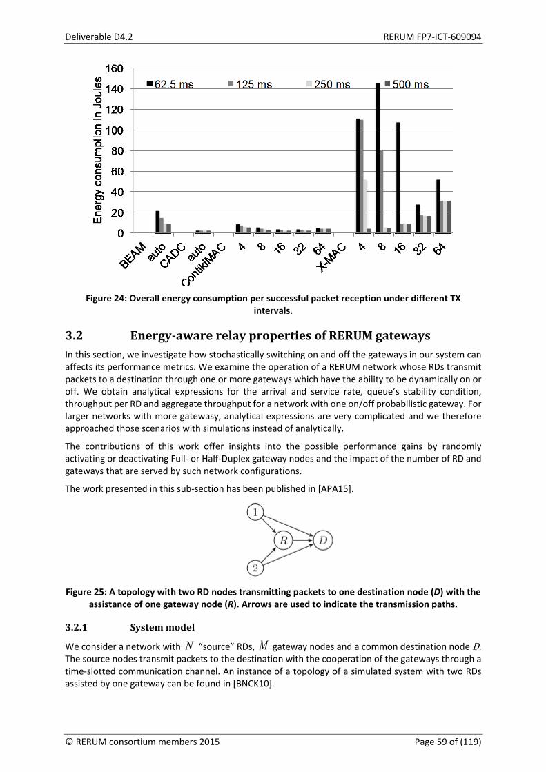
Deliverable D4.2 RERUM FP7-ICT-609094
Figure 24: Overall energy consumption per successful packet reception under different TX
intervals.
3.2 Energy-aware relay properties of RERUM gateways In this section, we investigate how stochastically switching on and off the gateways in our system can affects its performance metrics. We examine the operation of a RERUM network whose RDs transmit packets to a destination through one or more gateways which have the ability to be dynamically on or off. We obtain analytical expressions for the arrival and service rate, queue’s stability condition, throughput per RD and aggregate throughput for a network with one on/off probabilistic gateway. For larger networks with more gatewasy, analytical expressions are very complicated and we therefore approached those scenarios with simulations instead of analytically.
The contributions of this work offer insights into the possible performance gains by randomly activating or deactivating Full- or Half-Duplex gateway nodes and the impact of the number of RD and gateways that are served by such network configurations.
The work presented in this sub-section has been published in [APA15].
Figure 25: A topology with two RD nodes transmitting packets to one destination node (D) with the
assistance of one gateway node (R). Arrows are used to indicate the transmission paths.
3.2.1 System model
We consider a network with N “source” RDs, M gateway nodes and a common destination node D. The source nodes transmit packets to the destination with the cooperation of the gateways through a time-slotted communication channel. An instance of a topology of a simulated system with two RDs assisted by one gateway can be found in [BNCK10].
© RERUM consortium members 2015 Page 59 of (119)

RERUM FP7-ICT-609094 Deliverable D4.2
If a RD’s transmission to the destination fails, the gateways store the missed packet into the gateway’s queue which holds the less number of packets and try to forward it to the destination later. Transmitters have random access to the medium with no coordination among them and RDs’ queues are saturated with unlimited amount of traffic. A packet is transmitted in exactly one time-slot. Acknowledgements of successful transmissions are assumed instantaneous and error-free.
To simplify our analysis, we consider that the gateways do not generate packets by themselves and can transmit either in in-band Full- or Half-Duplex mode i.e. they can transmit and receive over the same frequency band either at the same time-slot or not respectively. We assume Multiple Packet Reception (MPR) for every receiver, the gateways, and the destination node; i.e. more than one transmitters can successfully send packets to the same destination in the same time-slot.
The wireless channel is modelled as Rayleigh flat-fading channel with additive white Gaussian noise. A RD’s transmission is successful if the received signal to interference plus noise ratio (SINR) is above a certain threshold γ . Small γ values are more likely to produce more successful simultaneous transmissions comparing to larger ones. For 1<γ the probability for two or more nodes transmitting successfully concurrently is higher than the same probability when 1>γ , which tends to zero [PET14].
Specifically, if there exists a set of T nodes transmitting at the same time-slot and ),( jiPrx is the signal power received from the transmitting node i at the receiver node j , then the ),( jiSINR
determined by node j is given by: ),(
),(=),(\
jkPnjiPjiSINR
rxiTkj
rx
∑ ∈+
, where jn is the receiver
noise power at j . Additionally, we assume that a packet transmitted by i is successfully received by
j if and only if 𝑆𝑆𝐼𝐼𝑁𝑁𝐴𝐴(𝑣𝑣, 𝑗𝑗) ≥ 𝛾𝛾𝑗𝑗 , where jγ is a threshold reflecting the transmission rate
requirements for node j .
Let )(iPtx be the transmitting power of node i and ),( jir be the distance between i and j . Then,
the power received by j when i transmits is ),(),(=),( jigjiAjiPrx , where ),( jiA is a unit-mean exponentially distributed random variable representing channel fading. The receiver power
factor ),( jig is given by α−)),()((=),( jiriPjig tx , where α is the path loss exponent with typical
values between two and four.
We consider the MPR case only with simulations since analytical expressions even for the case of one gateway are not at all tractable, see for example [PAT11].
3.2.2 Analysis
To facilitate the analysis of the model we simplified the system model and considered a network with N source RDs, one gateway node and a common destination node d . The link is modeled as a collision channel with erasures. Since simultaneous transmissions will result in collisions, the transmission probabilities can be tuned to reduce the number of collisions. In this section we consider the Half-Duplex case for the gateway.
The analysis we conduct here is based on [PTE10]. Let Niqi ,1,=, , be the probabilities with which every RD node attempts to transmit at every time-slot to avoid collisions. The gateway has an unsaturated queue and attempts to transmit with probability Rq , if its queue is not empty.
Let tiA be the event that the i -th’s RD node attempts transmission at time-slot t with probability
NiqAP iti ,1,=,=)( and
tRA denote the event that the gateway node attempts to transmit at time-
Page 60 of (119) © RERUM consortium members 2015

Deliverable D4.2 RERUM FP7-ICT-609094
slot t with probability: 0),>(=)( tonR
tR QPqqAP where
onq denotes the probability that the
gateway is enabled and tQ is the gateway’s queue size at time slot t , which is calculated as:
.,0)(=1 tttt XYQmaxQ +−+
Let ijO be the outage event between nodes i and j . When the signal to noise ratio, ijSNR , is below
a threshold γ , the link ij is in outage. Since the fading is assumed Rayleigh, the success transmission probability in link ij is:
)).(/),((=)(= 0 iPjirnexpOPp txijijαγ−
Note that events that are marked with bars are the complementary (not) events of the original. Let tX be a random variable which is equal to one, when there is addition of a packet into the gateway’s
queue at time slot t , or zero otherwise. Similarly, let tY be a random variable which is equal to one, when there is a packet removal from the gateway’s queue at time slot t , or zero otherwise. Therefore:
],)(1[=1=1=
tiR
tid
tj
N
ijj
tR
ti
N
i
t OOAAAX
≠
],)(1[=1=
tRd
ti
N
i
tR
t OAAY
where Ni ,1,= denotes the RD node, R the gateway node and d the destination. The evolution
of this infinite-state Discrete Time Markov Chain (DTMC) is depicted in Figure 26.
Figure 26: The DTMC which models the gateway’s queue size .
3.2.2.1 Arrival and service rate
The probability that the gateway holds at least one packet is 0)>( tQP . Let 0λ denote the arrival rate when the queue is empty and 1λ otherwise. The average arrival rate is
10 0)>(0)=(= λλλ tt QPQP + .
If the queue is empty, the arrival rate 0λ is:
).(1)(1=1=1=
0 j
N
ijj
iRidi
N
i
on qppqq −− ∏∑≠
λ (29)
tQ
© RERUM consortium members 2015 Page 61 of (119)

RERUM FP7-ICT-609094 Deliverable D4.2
If the queue is not empty, the arrival rate 1λ is 01 )(1= λλ Rq− . The average service rate seen by the gateway is:
).(1=1=
i
N
iRd
onR qpqq −∏µ (30)
To compute the probability of the gateway’s queue being empty, we need to solve the balance equations of the resulting DTMC in order to obtain the stationary distribution π 7.
The probability that the gateway’s queue is empty is:
.=0)=(01
1<1
λλµλµµλ
−−−tQP (31)
Thus, the average arrival rate is given by:
.)](1)(1[)(1
)](1)(1)[(1
=
1=1=1=
1=1=1=
j
N
ijj
iRidi
N
ii
N
iRd
j
N
ijj
iRidi
N
i
oni
N
iRd
qppqqp
qppqqqp
−−+−
−−−
∏∑∏
∏∑∏
≠
≠λ (32)
3.2.2.2 Gateway’s queue stability
If the queue is stable the departure rate is equal to the arrival rate. According to Loynes’ criterion [L62], the queue is stable if and only if the mean arrival rate is strictly less than the mean service rate, µλ <. Therefore we obtain:
,<)(1
1=0
0R
i
N
iRd
onq
qpq −+ ∏λ
λ (33)
which means that the queue is stable if Rq satisfies the inequality 1<< RRmin qq where:
.)(1)(1)(1
)(1)(1
=
1=1=1=
1=1=(1)
i
N
iRdj
N
ijj
iRidi
N
i
j
N
ijj
iRidi
N
i
Rmin
qpqppq
qppq
q−+−−
−−
∏∏∑
∏∑
≠
≠
3.2.2.3 Throughput per RD and aggregate throughput
Assuming the gateway’s queue is stable, the arrival rate from each RD node to the gateway is the
contributed throughput from it. Hence, the throughput rate iµ for the i -th RD when the gateway transmits in Half-Duplex is:
].)(1)[(10))>((1=1=
iRididj
N
ijj
tonRii pppqQPqqq −+−− ∏
≠
µ (34)
7 More details on calculating the stationary distribution can be found in [PTE10] and [PMET13].
Page 62 of (119) © RERUM consortium members 2015

Deliverable D4.2 RERUM FP7-ICT-609094
The aggregate throughput is defined as the sum of each RD’s throughput.
3.2.3 Simulation results
We performed a set of simulations in Matlab to assess the performance of different network topologies. We considered up to 30 RDs having the same link characteristics to gateways and destination and transmission attempt probabilities. With the intention of modeling the same link reliability among the different types of links, we used the same path loss exponents for each different link. Additionally, the transmission power of the gateways is five times the RDs’ one, while the value for the transmission probability of a gateway was chosen high enough to enforce the stability of each gateway’s queue. Every gateway attempts to transmit with the same probability and the same SINR threshold γ .
We simulated both the Full- and the Half-Duplex gateway modes. RDs were distributed randomly in a radius of m120 around the destination but not closer than m30 from the destination and m5 from each of the gateways. The presented results are averaged over 10000 time-slots. The values of the simulation parameters are listed in Table 4.
Table 4: Simulation parameters.
Symbol Explanation Value
Rdr gateway-destination distance m60
da RD-destination path loss exponent α 4
ra RD-gateway path loss exponent α 2
rra gateway-gateway path loss exponent α 4
rda gateway-destination path loss exponent α 2
)(iPtx transmit power of RD Ni ≤≤1 mW1
)( jtx RP transmit power of gateway Mj ≤≤1 mW5
iq RD transmission attempt probability 0.25
jRq gateway transmission attempt probability 0.85
The impact of the gateways’ on-probability parameter to several key performance metrics of the described network is discussed in the following sections.
3.2.3.1 Half-Duplex aggregate throughput
It is nearly always beneficial gateways to be always on 1)=( onq to maximize the aggregate throughput, which is the sum of the delivered packets to the destination, for the Half-Duplex relaying (Fig. 3). When RDs exceed five, switching gateways’ on-probability to 0.5 produces nearly half the aggregate throughput in comparison to the always on policy. Switching off the gateways completely
© RERUM consortium members 2015 Page 63 of (119)

RERUM FP7-ICT-609094 Deliverable D4.2
0)=( onq yields rather clos`e to always on performance, when five to 10 RDs are served by four gateways when the SINR threshold is 2.4=γ .
Another notable observation is that there are cases that keeping gateways switched off is far more beneficial than having them switched on with probability of one half. For instance, this is the case when four gateways serve four to 20 RDs with 2.4=γ or more than four RDs are served and 1.2=γ .
Figure 27: Aggregate Throughput vs # of RDs for different on-probability of the Gateways (top: full-
duplex, bottom: half-duplex).
3.2.3.2 Full-Duplex aggregate throughput
When two gateways assist RDs’ transmissions, it is better to operate always on. Having them operate with half the on-probability yields almost a 20% decrease to the delivered aggregate throughput, whereas a steep decrease in performance occurs when they are switched off.
When four gateways are operating, there are cases where setting the gateways’ on-probability at 0.5 results in a great increase in terms of the aggregate throughput in comparison to the alway-on policy, when RDs exceed seven. Moreover, in this case, the aggregate throughput remains constant when the number of RDs increase and the on-probability is one half. This is because links characterized by high γ values allow less concurrent successful transmissions to happen. Hence, it can be beneficial to switch off the gateways in such cases. As an example, observe the case where four gateways serve three to 20 RDs with the SINR threshold equal to 2.4 in Figure 27.
3.2.3.3 Average queue size
Average Queue Size vs RDs for different gateway on-probability values (two left: gateways transmitting in Full-Duplex mode, two right: gateways transmitting in Half-Duplex mode).
Delay vs RDs for different gateway on-probability values (two left: gateways transmitting in Full-Duplex mode, two right: gateways transmitting in Half-Duplex mode).
In the Full-Duplex mode, there exists a significant probability that the gateways attempt to transmit at every time-slot (Table 4). There is a substantial increase to the average queue size when the served RDs are increased for a low SINR threshold (Figure 28). This can be attributed to the high number of transmission attempts that happen along with the high success probability and the fact that the on-probability is equal to 0.5, which means that the packets remain to a gateway’s queue until it is
Page 64 of (119) © RERUM consortium members 2015

Deliverable D4.2 RERUM FP7-ICT-609094
switched on (at most half of the times in this case). Since the probability of success in a transmission is increasing with SINR, when 1.2=γ less concurrent successful transmissions happen in comparison to the 0.2=γ case, so the average queue size of the system is lower.
In the Half-Duplex mode, the average queue size remains under one when the SINR threshold is low (1.2<γ ), since gateways in Half-Duplex either receive or transmit simultaneously. Such a low value
can be justified by the fact that the gateways attempt to transmit with probability jRq (Table 4) and
hence they act as receivers with probability jRq−1 at each time-slot.
Figure 28: Average Queue Size vs #of RDs for different Gateway on-probability values (two left:
Full-Duplex, two right: Half-Duplex mode).
3.2.3.4 Delay
In Figure 5 we show delay, in number of time-slots it takes on average for a packet to be delivered to the destination, per packet versus the number of RDs.
Full-Duplex gateways exhibit a rapid increase to the delay per packet when the served RDs are increased. When the on-probability is equal to 0.5 and the SINR threshold is 1.2 the delay per packet is highly increased to the number of RDs, whereas when the gateways work in always on mode, the delay is greatly decreased. This fact is attributed to the fact that the gateways remain switched on (and transmitting with probability
jRq ) half of the time.
When the communication link is weak ( 2.4=γ ), then the two cases (always on vs 0.5=onq ) are comparable since in such a channel a few successful transmissions can occur. On the other hand, Half-Duplex gateways demonstrate a behaviour similar to that of the average queue size: the delay per packet increases to the number of RDs. The rate by which Half-Duplex gateways transmit compared to their receive rate justifies why there is no excess delay in such systems.
Figure 29: Delay in timeslots vs #of RDs for different Gateway on-probability values (two left: Full-
Duplex, two right: Half-Duplex mode).
3.2.4 Conclusion
In this sub-section, we presented the operation of energy efficient nodes relaying packets from a number of RDs to a destination node. We obtained analytical expressions regarding one gateway’s queue characteristics such as arrival and service rate, queue’s stability condition and per RD and aggregate throughput.
© RERUM consortium members 2015 Page 65 of (119)

RERUM FP7-ICT-609094 Deliverable D4.2
We simulated systems with one up to four gateways serving up to 30 RDs to gain insight the aggregate throughput, average queue size and packet delay of the system, since analytical expressions are not yet available. The results reveal that having Full-Duplex gateways switched on half of the time is beneficial when the communication channel is poor.
Page 66 of (119) © RERUM consortium members 2015

Deliverable D4.2 RERUM FP7-ICT-609094
4 Network Lifetime of Smart Object Deployments This section focuses on techniques that increase overall network lifetime by improving protocols at the network layer and by optimising multi-radio selection mechanisms.
More specifically, we firstly present an analysis of the energy consumption properties of a multicast forwarding algorithm for IPv6-based low-power wireless networks. The mechanism, developed by RERUM and first presented in D4.1 [RD4.1], achieves very low energy efficiency by reducing the amount of required network control messages. As we will see in further detail in Section 4.1, this method is particularly applicable to scenarios involving point-to-multipoint traffic.
Subsequently, in Section 4.2, we evaluate an energy-efficient multi-radio selection mechanism based on a scheme named “threshold-based selection diversity”. This scheme improves receiver performance compared to alternative approaches. The immediate result is reduced outage probability and reduced Bit Error Rates, both of which indirectly improve energy consumption.
4.1 Energy consumption of multicast forwarding with BMFA In scenarios involving point-to-multipoint network traffic, transmitting to each destination individually with unicast leads to (i) poor utilization of network bandwidth, (ii) excessive energy consumption caused by the high number of packets and (iii) suffers from low scalability as the number of destinations increases.
For UC-O2 - Environmental monitoring in particular, it is expected that networks will be formed by a potentially very high number of RDs and therefore scalability is a requirement. In cases when RDs are powered by batteries, it is impractical or outright untenable to replace batteries very frequently due to high management cost and possibly hard-to-reach installation locations. Thus, long battery life is important. For devices powered from mains, low energy consumption is also important in order to reduce financial cost, but also in order to comply with national and international regulations where applicable.
For those reasons, RERUM has designed and implemented the Bi-Directional Multicast Forwarding Algorithm (BMFA) for 6LoWPANs. BMFA addresses the needs of RERUM use-cases by achieving very low energy consumption. This section presents a thorough performance and energy consumption evaluation of the BMFA multicast forwarding algorithm, which was developed during Task 4.2 and introduced in RERUM deliverable D4.1 [RD4.1].
Through the phase of the experiments we are targeting not only showing comparative results between our algorithm BMFA and its rival Trickle Multicast / Multicast Protocol for Low power and Lossy Networks (TM / MPL), but also to identify their overall behaviour when they are subjected under different configurations. In [OP12, OPT13], the authors discuss Stateless Multicast RPL Forwarding (SMRF)’s primary limitation, which is that it can only forward traffic “downwards” the RPL tree. A corollary of this limitation is that if the multicast traffic source is not the root of the tree, then traffic would never be able to reach nodes belonging to specific sub-trees. From one point of view we want to keep the structure of the experiments similar to the one in [OP12, OPT13], in order to be able to maintain comparability. On the other hand, by making some modifications we can see the overall behaviour of the two algorithms regardless of the source's positions and the number of sinks in the network.
With those in mind, this section is structured as follows: We start with a description of the parameters used for our simulations in Section 4.1.1. Subsequently, in Section 4.1.2, we document the environment used for our simulations, we present results and we discuss our findings.
© RERUM consortium members 2015 Page 67 of (119)

RERUM FP7-ICT-609094 Deliverable D4.2
4.1.1 Network configuration parameters
As we have seen in [OP12, OPT13], the performance of the algorithms strongly depends on a number of parameters whose values can vary based on the sub-network properties. In this section we are about to discuss the different parameters and their meaning in the experiments.
4.1.1.1 Network density
In a network of statically-deployed nodes and without mobility support, the term Network Density (ND) is defined in the same way as the density of an undirected graph with edge set E and vertex set
V. Thus: )1(
2−
=VV
END . ND = 0 for an edgeless graph and ND = 1 for a complete graph. In this
context, we consider symmetric graphs where an edge between two nodes exists if and only if they can hear each other; in other words they are single-hop neighbours.
Network Density is a link layer metric: an edge between nodes A and B exists if and only if the two nodes are single-hop neighbours (can directly hear each other). This definition only makes sense if radio links are symmetric, which is true for Cooja's Unit Disk Graph Medium (UDGM) environment, but not always the case for real deployments. In case of non-symmetric links (e.g. when A can hear B, but B cannot hear A due to e.g. different transmission powers), the link layer topology would have to be modelled as a directed graph. Investigating the behaviour and performance of multicast algorithms in an environment with non-symmetric links is part of our future plans.
In the context of BMFA, the network is created based on an Objective Function (OF) [VKPD+12], which defines how RPL [WTBH+12] nodes select and optimize routes. In a nutshell, a node (A) selects its preferred parent between candidates B and C based on the perceived quality of the links between A and B / A and C respectively. Different OFs use different metrics to estimate link quality, such as Expected Transmission (TX) Count (ETX) or latency. When ND increases, so does the number of candidate parents a node can select among, while end-to-end hop count also decreases. Consequently, this is expected to lead to higher Packet Delivery Ratio (PDR) and lower End-to-End Delay (EtED).
Due to its per-packet storing nature, TM is a path-redundancy aware algorithm and its efficiency increases as the Network Density gets higher. Neighbouring nodes exchange information about their cache contents through control messages, governed by t [LCHG11, LPCS04] timers, in order to decide whether they share the same information. If not, the packets that cause the disagreement are forwarded almost immediately. By increasing the Network Density, the probability of a specific packet not reaching a specific node decreases since more neighbouring nodes are in range to forward that packet. However, a drawback is that wireless collisions can occur when multiple nodes are transmitting simultaneously. Even though some randomness is added to the forwarding delay so that such situations can be avoided, it is very likely that the receiver node is going to be hearing noise, leading to packet loss.
For our experiments, we have randomly selected networks of three different densities; 0.14 (low), 0.35 (intermediate) and 0.72 (high). Figure 30 depicts the signal coverage for the three densities (dark blue; light blue; dotted circles respectively). Nodes with a solid black fill act as multicast sources.
4.1.1.2 Forwarding delay
In the context of ContikiMAC [D11], SMRF [OP12, OPT13] introduced a cross-layer optimization so as to improve its overall performance. When a node receives a multicast frame, instead of forwarding it directly, it introduces a short delay D = (Fmin, CCI), where Fmin is a configuration parameter. Setting this parameter to a positive value is especially useful, for example, in the case where the underlying duty cycling algorithm never turns its radio off. If a node attempts to forward the packet before the sender has gone through the entire packet train (section 3.1.2), then a collision would occur and the outgoing packet would be dropped. In order to ensure that such a collision would not exist, the packet
Page 68 of (119) © RERUM consortium members 2015

Deliverable D4.2 RERUM FP7-ICT-609094
transmission should be delayed by at least CCI ms. This holds because if the receiver has waken up just on time when the first packet of the chain arrived, then he has to wait for exactly CCI ms, the time the sender needs to go through the entire packet train. Since ContikiMAC's default CCI is set to 125ms, we can arbitrarily set Fmin to a value <=125ms. Furthermore, SMRF can optionally delay the packet forwarding by a random factor in order to mitigate the hidden terminal effect. The final delay is a random value in [D, Spread*D] where Spread is a positive integer. Note that by increasing the Spread, the End-to-End delay is expected to be higher. BMFA inherits both of these methods.
Figure 30: Simulated topologies.
On the other hand, TM [HK14] is governed by trickle timers [LCHG11, LPCS04], in order to efficiently propagate state information with control messages without flooding the network. Upon a control message reception, if an inconsistency is found, the timer interval I is reset to Imin and the packets causing it are transmitted within a short delay. In order to mitigate signal collisions and the hidden terminal effect, the final delay is a random value in [I/2, I]. As Imin increases it is expected that the End-to- End delay is going to be higher. On the opposite direction, where Imin is too low, signal collisions are more likely to happen causing higher packet loss. This holds since the interval [I/2, I] that provides the randomness shrinks as the value of I is reduced.
For our experiments we have selected two and three different forwarding delays for BMFA and TM respectively. For BMFA, two different spreads are used (2 and 4) in combination with an initial delay of 125ms; the one used by ContikiMAC. For TM, the three forwarding delays are 125ms, 500ms and 700ms.
4.1.1.3 Transmission bit rates
In the context of 6LoWPANs where the resources are limited, the transmitting bit rate can reveal the constraints a node faces in the network. One of the main problems is the limitation of the storage each node has and by increasing the bit rate we can check at what point the cache overflows leading to packet drop.
Since TM does not maintain any network topology information, in order to support IPv6 multicasting, every node maintains a cache of recently seen packets uniquely identified with the help of a Hob-by-Hop Option (HBHO) extension header. Upon a packet reception, if its HBHO indicates that it does not already exist in the cache, it gets added. To avoid flooding the network with unnecessary transmissions, after their reception, packets are not forwarded directly. Nodes wait to exchange Internet Control Message Protocol v6 (ICMPv6) control messages and, if they disagree on their contents, they forward
1
9
10
© RERUM consortium members 2015 Page 69 of (119)

RERUM FP7-ICT-609094 Deliverable D4.2
the packets causing the disagreement. If the frequency of transmission rate is relatively high to the frequency that the control messages are exchanged then the cache is very likely to overflow. Existing packets will be overwritten by newly arrived ones and will never get forwarded to the next node. Thus, assuming a constant frequency of control messages exchange, the Packet Delivery Ratio is expected to decrease as the transmitting bit rate increases.
Despite the fact that BMFA does not make use of such a cache, we can examine how Bit Rate can affect the network's efficiency from another perspective. In [AFRA+13] the authors proposed a method for retaining low packet loss when a member node moves at the limit of the signal coverage boundaries. To put it in another way, when the quality of signal between two nodes is poor, the transmission rate must be lowered in order to achieve higher Packet Delivery Ratio. In 6LoWPANs where the links are lossy, experimenting with different values of bit rate will expose the limitations the two algorithms face in such networks.
The values used as inter-packet delay for our experiments are 250ms, 500ms, 750ms and Variable Bit Rate (VBR), which represents a random choice between 1s and 2s.
4.1.1.4 Source positions
In [OP12, OPT13] we have seen that the node acting as multicast source was positioned at the top node of the network, the one which was acting as the RPL root. As we mentioned above, this was obligatory in order all nodes to be able to participate as sinks. While BMFA omits this constraint, we can see how different positions of the source node can affect metrics such as Packet Delivery Ratio, End-to-end Delay and Energy Consumption.
In the case of BMFA where a packet is forwarded only once by a node, it is expected that the lower position of the source in the tree, the more effort is required overall by the network in order the packet to reach all destinations. When the source is at the RPL root, the distance a packet must cover to reach all subscribed destinations is equal the depth of the tree. On the other hand, a source positioned at a lower level has no knowledge whether multicast members exist above it. Thus a packet must be forwarded upwards until it reaches a node that is aware of membership existence in its other sub-trees. Then the packet is forwarded downwards to reach all subscribed nodes. In this case, the packet has to travel, at maximum, twice the distance of the tree’s depth resulting to higher End-to-end Delay and Energy Consumption. In addition, the Packet Delivery Radio is expected to decrease since it is more likely for a packet to be dropped at an intermediate node due to cache overflow or bad quality of link.
Since TM does not rely on the RPL structure and any multicast datagram is treated as a network- wide broadcast, moving the source node towards the “middle” of the network is expected to yield improvement to all metrics. This holds based on the fact that less hop-by-hop transmissions are needed so that a packet can arrive to all destinations.
For our experiments nodes 1, 9 and 18 (Figure 30) were selected to act as multicast sources (one of them per experiment).
4.1.1.5 Sink node count
Another factor that can potentially influence the efficiency of the two algorithms is the number of sinks that exist in the network. We have already mentioned that TM treads every multicast datagram as a network-wide broadcast, meaning that the datagram will eventually reach across all the network regardless if it is needed or not. Thus, the number of subscribed nodes will not play any role in TM's efficiency. For BMFA this is not the case. As the number of sinks gets higher it is more likely that they are going to be scattered in a larger range. This means that the probability of having a sink in each sub-tree of the Destination-Oriented Directed Acyclic Graph (DODAG) increases and consequently more effort will be required by the network to deliver a packet to all subscribed nodes. Similarly to the case of the Source Positions, this is expected to lead to higher End-to-End Delay, Energy Consumption and Packet Loss.
Page 70 of (119) © RERUM consortium members 2015

Deliverable D4.2 RERUM FP7-ICT-609094
For our experiments three randomly-selected sets of 5, 9 and 15 nodes out of 21 were chosen to act as sinks. The specific nodes composing each set were randomly selected once and used throughout all the experiments.
4.1.2 Experiment environment and results
For our evaluation we use the Cooja simulator [O06]. It allows the emulation of real hardware platforms in a simulated IEEE 802.15.4 wireless network. Our setup consists a number of nodes as discussed previously, with each one of them running either BMFA or TM as multicast forwarding algorithm. On a higher level, each node was also assigned a role in the network such as being a sink node, a source node or a simple traffic forwarder; the latter is a node that is not subscribed to any multicast groups but that is capable of interpreting and forwarding multicast traffic. Moreover, we simulated our network to run with the Unit Disk Graph Medium (UDGM) which models wireless losses based on distance. We configured UDGM so that each node had a TX range of 50m and an interference range of 60m Figure 31.
Figure 31: Simulated topology and transmission range within Cooja.
Throughout all experiments we measured the following metrics:
• End-to-End Delay • Energy Consumption
In this deliverable we discuss results related with energy consumption. End-to-End delay and other metrics are discussed in D4.3. Table 5 summarises the simulation parameters selected, as discussed throughout the previous section.
Table 5: Configuration of BMFA / TM simulations.
Node Count 21 motes (1 traffic source, 20 sinks) Radio Medium Unit Disk Graph Medium (UDGM)
Ranges TX: 50m, Interference: 60m PHY and MAC IEEE 802.15.4 with CSMA Duty Cycling ContikiMAC (CCI 125ms) & NullRDC
Random Seeds New seed each iteration Traffic Pattern CBR and VBR (rates discussed in text)
TM Imin in 125, 500, 700 ms BMFA Spread in 2, 4
Through the facilities provided by Contiki’s energy consumption estimation module (energest) [DOTH07a, DOTH07b], we measured the time each node spent in each of the following three states over the duration of each experiment: i) MCU active, ii) RF listening / receiving, iii) RF transmitting. Since we are simulating the exp5438 (Texas Instruments (TI) MSP430F5438 experimenter board) [TI14, TI07], we then converted these time values to estimated energy consumption based on typical datasheet power levels at an operating voltage of 3.0V. This includes the consumption of the Micro-
© RERUM consortium members 2015 Page 71 of (119)

RERUM FP7-ICT-609094 Deliverable D4.2
Controller Unit (MCU), a Texas Instruments (TI) MSP430F5438 [TI14], as well as the consumption of the TI CC2520 radio transceiver [TI07]. The values are summarised in Table 6.
Table 6: Typical exp5438 current draw with an operating voltage of 3.0V at 25oC.
Mode Current Consumption MCU active @ 8MHz, Code execution from Flash 2.50mA
MCU in Deep Sleep (LPM3, XT1LF TI14) 2.60μA CC2520 Frame Reception at an input level of -50dBm 18.5mA
CC2520 Frame Transmission, 0dBm output power 25.8mA
NullRDC keeps radio transceivers always on (no duty cycling). As a result, the majority of energy is consumed during idle listening or packet reception, with other components contributing insignificantly. For this reason, we only consider ContikiMAC for the evaluation of the two algorithms in terms of energy consumption. Generally for TM it can be observed (Figure 32) that for higher densities less energy is consumed due to the fact that agreement between all nodes can be achieved with fewer ICMPv6 control message exchanges; in other words inconsistencies can be solved with fewer hop-by-hop transmissions. This can be also observed by the fact that as the density increases less energy is required for transmitting than for listening.
Figure 32: BMFA vs TM average node energy consumptions.
For BMFA, irrespective of network density, as the inter-packet delay between the transmitted packets increases, the energy consumption decreases since fewer packets are forwarded during the experiment. In the case of the highest density (0.71) and for high bit rate we can see that the energy consumption of BMFA approaches the one of TM's. This happens because nodes are consuming too much energy by keeping the radio on as a result of picking up transmissions from their large number of neighbours, despite the fact that they only forward packets received only from their children or preferred parent. By comparing the two algorithms we can see that BMFA is more energy efficient than TM since it forwards each packet only once and there is no ICMPv6 message exchange. Moreover, we must highlight that the energy consumption for CPU indicates the complexity of the two algorithms and it becomes noteworthy that TM's complexity is much higher than BMFA's. Generally, BMFA can outperform TM in energy efficiency especially in low density networks where TM consumes four times
Page 72 of (119) © RERUM consortium members 2015

Deliverable D4.2 RERUM FP7-ICT-609094
more energy; and assuming that TM can be configured to achieve higher PDR, its energy consumption is expected to be even higher.
4.2 Adaptive and energy-efficient multi-radio selection mechanisms
4.2.1 Introduction
The energy consumption of telecommunications systems highly depends on the radio-access technology (e.g., WiFi, Zigbee) that is employed. At the same time the radio-access technology determines the bit-rate and also the bit-error rate. In this sense, the option to switch dynamically between different radio-access technologies results in systems that can optimize their operation mode in order to achieve the desired trade-off between energy consumption and bit rate (or bit error rate). In this way the benefits of different technologies can be combined towards an improved Quality-of-Service (QoS) and more efficient resources utilization. However, multi radio-access systems require the monitoring of the different radio-links/diversity-paths (e.g., periodic measurement of the signal-to-noise ratio (SNR))
In many practical situations, though, the continuous monitoring of all the available diversity paths, leads to unnecessary resources consumption, such as control channels. A common practice, which compromises between resources consumption and performance improvement, is to employ adaptive diversity mechanisms. One such attractive solution for various wireless communication scenarios is the selection diversity (SD), which offers relatively low complexity and improved performance. In the context of low complexity diversity methods, several approaches have been proposed, which, apart from the SD receiver, they include the switch-and-stay combining (SSC) and switch-and-examine combining (SEC) schemes [SA05]. SEC has been designed to bridge the gap between SD, which provides the best performance, and the least complicated SSC, which however gives the poorer performance. Nevertheless, since SEC does not take full advantage of the available path estimates, its performance is closer to the SSC one. However, despite the fact that diversity reception improves the QoS, it also increases the complexity as well as the data overhead. The latter one significantly increases with the number information that must be shared among the network elements for performing various operations, e.g., channel state information (CSI) estimation [ALH12, LBA13].
Recently, a new diversity reception technique, which enables efficient and effective communications among the wireless networks elements, was proposed [BR14]. In that scheme, named threshold-based selection diversity (t-SD), the receiver uses the current path as long as its SNR is above a predefined threshold. Whenever the SNR of the selected path falls below the threshold, it switches to (selects) the diversity path that provides the largest instantaneous SNR. As a consequence, the receiver’s performance clearly improves, as compared to SEC, and thus approximates more closely the corresponding one of SD. In addition, it is shown that the induced system complexity, in terms of the average number of path estimations (ANPE) as well as the switching probability (SP), are kept relatively low. Therefore, in many cases t-SD outperforms the conventional receivers in terms of performance, complexity and energy/cost efficiency trade-off. Based on this new diversity scheme, we investigate its performance under more realistic wireless environments modelled in our case using the Nakagami-m fading model [SA05].
The work discussed in this sub-section has been published in [LM14].
4.2.2 Mode of operation
Let us consider the downlink of a communication system with one transmit and L receiving antennas. In the scheme under consideration, the receiver examines periodically, whether the received SNR of the path that was selected in the previous time slot (e.g., γi with I ∈ 1,2,…,L) exceeds a predefined
threshold γth. If that path exceeds the threshold, the receiver continues using this path, otherwise it
© RERUM consortium members 2015 Page 73 of (119)
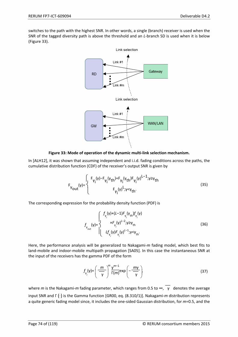
RERUM FP7-ICT-609094 Deliverable D4.2
switches to the path with the highest SNR. In other words, a single (branch) receiver is used when the SNR of the tagged diversity path is above the threshold and an L-branch SD is used when it is below (Figure 33).
Figure 33: Mode of operation of the dynamic multi-link selection mechanism.
In [ALH12], it was shown that assuming independent and i.i.d. fading conditions across the paths, the cumulative distribution function (CDF) of the receiver’s output SNR is given by
Fγout(γ)=
Fγi
(γ)−Fγi(γth)+Fγi
(γth)Fγi(γ)L−1;γ≥γth
Fγi(γ)L;γ<γth.
(35)
The corresponding expression for the probability density function (PDF) is
fγout(γ)=
fγi(γ)+(L−1)Fγi
(γth)fγi(γ)
×Fγi(γ)L−2;γ≥γth
Lfγi(γ)Fγi
(γ)L−1;γ<γth.
(36)
Here, the performance analysis will be generalized to Nakagami-m fading model, which best fits to land-mobile and indoor-mobile multipath propagation [SA05]. In this case the instantaneous SNR at the input of the receivers has the gamma PDF of the form
fγi(γ)=
m
γ
m
γm−1
Γ(m)exp
−
mγ
γ , (37)
where m is the Nakagami-m fading parameter, which ranges from 0.5 to ∞, γ denotes the average
input SNR and Γ ( )⋅ is the Gamma function [GR00, eq. (8.310/1)]. Nakagami-m distribution represents a quite generic fading model since, it includes the one-sided Gaussian distribution, for m=0.5, and the
Page 74 of (119) © RERUM consortium members 2015

Deliverable D4.2 RERUM FP7-ICT-609094
Rayleigh distribution, for m=1, as special cases. In the limit as m→∞, the Nakagami-m fading channel converges to a non fading additive white Gaussian noise (AWGN) channel. The corresponding expression for the CDF of γi is given by
Fγi(γ)=1−
Γ ( )m,mγ/ γ
Γ(m) , (38)
where Γ(⋅,⋅) is the upper incomplete Gamma function [GR00, eq. (8.350/2)]. Therefore, substituting (38) in (35) yields the following closed-form expression for the CDF of γout
Fγout(γ)=
Γ
m;
mγth
γ −Γ
m;
mγ
γ
Γ(m) +
1−
Γ
m;
mγth
γ
Γ(m)
×
1−
Γ
m;
mγ
γ
Γ ( )m
L−1
;γ≥γth
1−
Γ
m;
mγ
γ
Γ ( )m
L
;γ<γth.
(39)
Assuming integer values for m, based on [GR00, eq. (8.352/2)] and using the binomial and multinomial identities, [GR00, eq. (1.111)] and [AS72, eq. (24.1.2)], respectively, the corresponding PDF expression can be expressed as
© RERUM consortium members 2015 Page 75 of (119)

RERUM FP7-ICT-609094 Deliverable D4.2
fγ
out
(γ)=
exp
−
mγ
γ ( )m/ γ
m
Γ(m) γm−1
+
1−exp
−
mγth
γ ∑
i=0
m−1 ( )mγ
th/ γ
i
i!
× ∑i=1
L−1 L−1i(−1)i ∑
n0;…;n
m−1
i ∏
k=1
m−1
(m/ γ )k
k!
nk
×
∑k=1
m−1 kn
kγ ∑
k=1
m−1 kn
k−1exp
−
mi
γ γ
−
mi
γ γ ∑
k=1
m−1 kn
kexp
−
mi
γ γ ;γ≥γ
th
∑i=0
L Li(−1)i ∑
n0;…;n
m−1
i ∏
k=1
m−1
(m/ γ )k
k!
nk
×
∑k=1
m−1 kn
kγ ∑
k=1
m−1 kn
k−1exp
−
mi
γ γ
−
mi
γ γ ∑
k=1
m−1 kn
kexp
−
mi
γ γ ;γ<γ
th
. (40)
Substituting (40) in the definition of the Moment-Generating Function (MGF), i.e., Mγout
(s)=E⟨exp(−sγout)⟩, with E < >⋅ denoting expectation, and using [GR00, eqs. (3.351/1 and 3.351/2)]
yields the MGF of γout given in (41). In that equation, γ(⋅,⋅) denotes the lower incomplete gamma
function [GR00, eq. (8.350/1)].
(41)
4.2.3 Performance
In this section, using the previously derived expressions for the PDF, CDF, MGF and moments of the output SNR, various performance evaluation criteria will be presented, such as the Outage Probability (OP), ABER and ASNR, complemented by a complexity analysis.
Page 76 of (119) © RERUM consortium members 2015

Deliverable D4.2 RERUM FP7-ICT-609094
4.2.3.1 Outage probability
OP is defined as the probability that the SNR falls below a predetermined threshold γT and is given by
Pout=Fγout(γT).
High SNR approximation: In order to clearly understand important system-design parameters, we focus here on the high SNR regime. This approach helps us to quantify the amount of performance variations, which are due to the fading effects as well as to the receiver’s architecture. At high SNR regime, the upper incomplete gamma function can be approximated as Γ(m,x)≈Γ(m)−xm/m , as 0x→ [AS05]. Based on this approximated expression, the CDF of γout, in the high SNR regime, can be written
as follows:
Fγ
out
(γ)≈
( )m/ γ
m
mΓ(m) ( )γm−γmth
+γmth
( )m/ γ
m
mΓ(m)
L
γm(L−1);γ≥γth
( )m/ γ
m
mΓ(m)
L
γmL;γ<γth
.
(42)
4.2.3.2 Average Bit Error Rate (ABER)
Using the previously derived MGF expression in (41) and following the MGF-based approach, the ABER can be readily evaluated for a variety of modulation schemes]. More specifically, the ABER can be calculated: i) directly for non-coherent differential binary phase shift keying (DBPSK), that
is PDBPSKbe =0.5Mγout
(1); and ii) via numerical integration for Gray encoded M-PSK, that
is PM−PSKbe =
1πlog2M ⌡⌠
0
π−π/M Mγout
log2Msin2 ( )π/M
sin2φ dφ.
High SNR approximation: Considering higher values of the average input SNR and based on (42), yields the following simplified expression for the PDF of the output SNR
fγ
out
(γ)≈
( )m/ γ
m
Γ(m) γm−1+γmth
( )m/ γ
m
mΓ(m)
L
×[m(L−1)]γm(L−1)−1;γ≥γth
( )m/ γ
m
mΓ(m)
L
mLγmL−1;γ<γth
.
(43)
For γth≈ γ , the diversity gain is mL, since the sum terms with the upper incomplete gamma functions
have negligible effect on the performance. On the other hand, for γth≪ γ , the diversity gain is m,
since the sum term with the lower incomplete gamma function has negligible effect on the performance. This means that, depending on the switching threshold, the hybrid receiver under investigation switches between a pure SD and a single receiver, respectively.
© RERUM consortium members 2015 Page 77 of (119)

RERUM FP7-ICT-609094 Deliverable D4.2
4.2.3.3 Average Output Signal-to-Noise Ratio
The ASNR is an important performance indicator that is tightly related to the performance metrics of a system, such as the ABER and the asymptotic spectral efficiency. ASNR can be directly evaluated by setting n=1 in (44):
(44)
4.2.4 Complexity
The complexity of the scheme under consideration will be investigated by employing the Average Number of Path Estimations (ANPE) and the SP in a guard period as a quantification of the power savings [LKT08, YA06].
4.2.4.1 Average Number of Path Estimations
The system complexity increases as the ANPE increases, due to the important amount of information that must be exchanged for performing various operations, e.g., channel estimations. In [BR14], it was shown that the Average Number of Path Estimations (ANPE), Nout, is given by
Nout=1+(L−1)Fγi(γth). (45)
4.2.4.2 Switching Probability (SP)
SP is an important performance measure that is very useful in practical scenarios. In particular switching between branches not only consumes power, but also reduces the data throughput in a transmit-switched diversity configuration as well as leads to inaccurate phase estimates. Also in [BR14]
it was shown that the SP, Psout, can be expressed as
Psout=Fγi
(γth)
1−
1LFγi
(γth)L−1 . (46)
4.2.5 Results
Based on the previous derived analysis, various numerical performance evaluation results will be presented. In Figure 34, the OPs of dual-branch SD and t-SD receivers are plotted as a function of the
switching threshold, γth, assuming normalized outage threshold, γT/ γ =−5dB. In the same figure, the
SP, Psout, and the ANPE, Nout, are also included. It is depicted that for higher values of γth, the OP of t-
SD becomes almost equal to the corresponding one of SD. However, for these high values of γth, Nout
as well as Psout of t-SD are considerably lower as compared with the corresponding ones of SD.
Therefore, based on the proposed receiver, non-negligible energy savings are expected without any important loss in performance.
Page 78 of (119) © RERUM consortium members 2015

Deliverable D4.2 RERUM FP7-ICT-609094
Figure 34: Performance in terms of OP, SP and Path estimations.
In Figure 35 considering L=3 diversity branches, the ASNRs of SD and t-SD are plotted as a function of
the average input SNR, γ , and for various values of the Nakagami shaping parameter m. It is depicted
that for lower values of γ , the ASNR performance is equal, while a performance gap appears when
γ >γth, with SD having always the best performance. In this figure, it is interesting to note that the
ASNR decreases as the severity of fading decreases (i.e., m increases), which seems to be surprising at first sight. However, the main reason for this behavior is that as m increases, the distribution becomes more skewed, which reduces the effective area of integration and therefore explains this dependence of the average SNR on the fading parameter. In the same figure, for the same values of L and γth, a
table containing Nout of the previously tested diversity schemes, is also included. In this table, it is
shown that t-SD requires quite lower values for the ANPE, especially for γ >γth. More specifically, for
γ ≈γth, t-SD seems to constitute the optimal solution for the trade-off between performance and
complexity.
In order to highlight the above mentioned trade-off, in Figure 36, the minimum ABER, Pbe, is evaluated
for SD and t-SD, assuming that a constraint, Nc, on the ANPE exists.
Setting constraints on the number of path estimations is expected to considerable decrease the system complexity as well as increase the effective throughput, since lower feedback information will be
exchanged between source and destination. Thus, in this figure, assuming DBPSK, γ =6dB, the
minimum Pbe is illustrated as a function of Nc, for various values of γth. In all cases, it is shown that the
performance improves as the constraint on ANPE is relaxed. However, the selection of γth is off critical
importance, since for γth> γ , the minimum Pbe, satisfying the constraints, is provided with t-SD. In
© RERUM consortium members 2015 Page 79 of (119)

RERUM FP7-ICT-609094 Deliverable D4.2
the same figure, assuming γth=6dB, a table containing the SPs of t-SD and SD is also included. In this
table, it is shown that t-SD provides always the smallest SP. Lastly, computer simulation performance results are also included in all figures, verifying the validity of the proposed theoretical approach.
Figure 35: ASNR and average number of path estimations of SD and t-SD.
Figure 36: ABER performance and complexity trade off analysis.
Page 80 of (119) © RERUM consortium members 2015

Deliverable D4.2 RERUM FP7-ICT-609094
5 Energy Consumption and Security Trade-offs Among RERUM’s key contributions are a number of lightweight, energy-efficient security mechanisms suitable for execution on constrained environments and devices such as RDs. Security mechanisms impose computational and communication overhead, and this has a negative impact on overall lifetime of a battery-powered device. This section focuses on evaluating the trade-offs between energy efficiency and security for some of the RERUM-developed mechanisms.
More specifically, we start with the power consumption evaluation of a RERUM-developed privacy-preserving authorization mechanism (Section 5.1). The evaluation focuses on Class 1 Devices (about 10 KB RAM and around 100 KB Flash). This mechanism was recently presented at the IETF’s Authentication and Authorization for Constrained Environments (ACE) working group.
Subsequently, we conduct energy consumption evaluation of JSS, the JSON Signatures Scheme developed as part of RERUM’s T3.1 and documented in D3.1 [RD3.1]. This scheme has been implemented with the Contiki OS in a platform-independent fashion. We undertake this evaluation with simulations and present our results in Section 5.2.
5.1 Power consumption evaluation of authorization mechanisms
5.1.1 State of the art authorization mechanisms
The problem of authorizing (constrained or unconstrained) clients to access directly resources provided by constrained servers in an end-to-end IP-based fashion over standard protocols like CoAP [SHB14] (and in particular, without the support of an application gateway) is not a trivial topic.
As many chip manufacturers claim, it is indeed probably true that many current solutions based on complex key agreement protocols and cryptographic mechanisms (DES, Elliptic Curves, AES [FIPS01], 3DES, and Kerberos − possibly via the creation of a secure DTLS [RM12] channel) are viable in the sense that there are appearing many chips designed for IoT use that do support the methods.
Nevertheless, as also discussed at the IETF meeting in Prague in July 2015, some of those solutions do consume energy resources at the constrained device. Our point of view is that it is indeed a great difference if user has to change the batteries of his devices every day, every week or every month. In particular, the low-budget, low-effort IoT application areas will still strongly profit from a major reduction in power consumption.
There is no real consensus on the question which protocols/methods consume how much energy on which hardware (the ACE WG will probably maintain an open document containing different measurements).
5.1.2 Energy consumption estimation of cryptographic algorithms on Class 1 devices
We measure the energy consumption of cryptographic algorithms (SHA256, AES, 3DES and ECDSA (Sign and Verify) on resource-constrained devices, which own limited memory and CPU, considering mainly the class 1 devices with about 10 KB RAM and around 100 KB FLASH. We have used for this purpose a MSP430 LauchPad with a MSP430F5529 microcontroller, which has 8KB RAM and 128KB Flash. The microcontroller has no hardware accelerator for any cryptographic algorithms. The used cryptographic functions come from the cryptographic system library of an open source project RIOT8. It provides a friendly operating system for the Internet of Things.
8 https://github.com/RIOT-OS/RIOT
© RERUM consortium members 2015 Page 81 of (119)

RERUM FP7-ICT-609094 Deliverable D4.2
The used measurement tool is an oscilloscope, which can be used to observe constantly varying voltage signals over time. To calculate the energy consumption E, voltage V, current I and duration t need to be known. The working voltage V of the microcontroller can be simply measured by connecting its VCC to the oscilloscope with its GND as reference. The current I can be measured with the help of a 10 ohm resistor R: I = V10R / 10. An output pin of the microcontroller is used as signal to mark the duration t of an operation. The power supply of the microcontroller is 3 AA batteries. The whole measurement setting can be found in the next Figure.
Figure 37: Measurement settings.
The measurement data, over time, for the four cryptographic algorithms are plotted in the next two Figures (Figure 38 and Figure 39). The purple lines show the electric current, the green lines the voltage on the microcontroller VCC and the blue lines the voltage of the trigger signals. During a cryptographic operation, the trigger signal is about 0 V. When an operation is finished, the trigger signal gives the same voltage as the VCC. The unit of the X-axis is seconds The Y-axis is in Milliampere for electric current, and in Volt for the VCC and trigger signals.
Using Gnu Octave, the whole data are processed to calculate the energy consumption using the following form:
(47)
where
E: Energy consumption
t: Duration of an operation
n: Number of simples
Vi: VCC voltage value of i-th sample
Ii: Current value of i-th sample
Page 82 of (119) © RERUM consortium members 2015
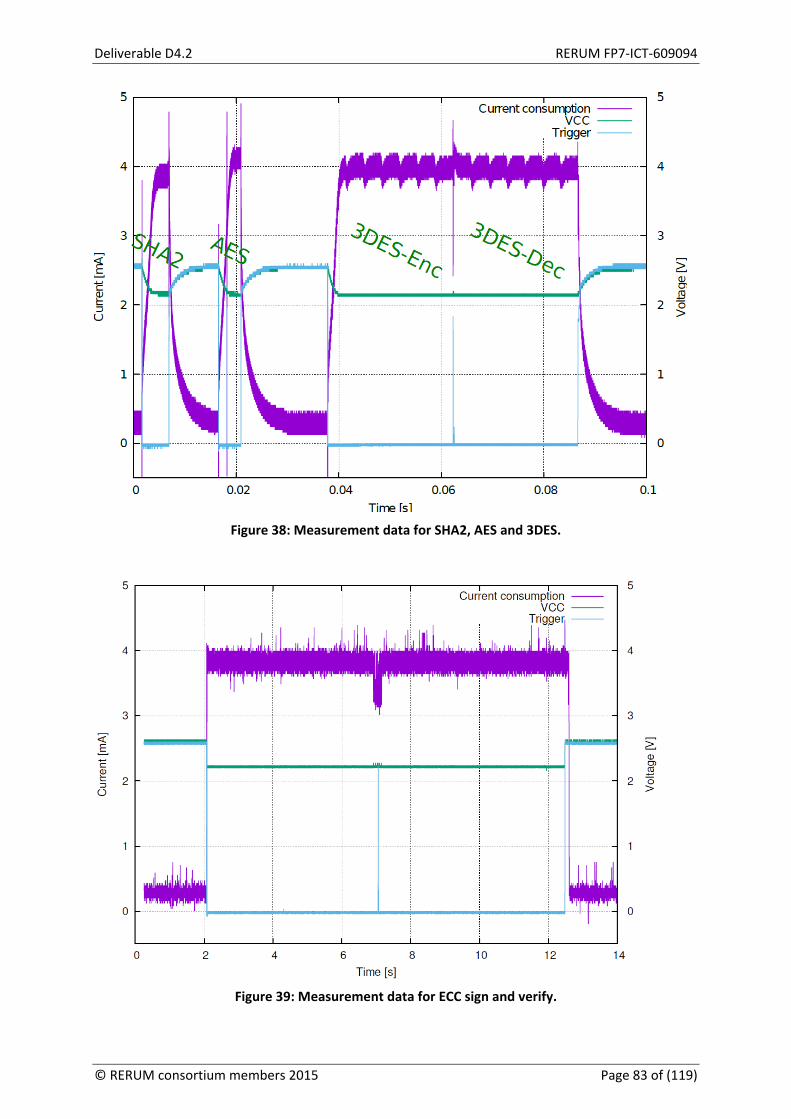
Deliverable D4.2 RERUM FP7-ICT-609094
Figure 38: Measurement data for SHA2, AES and 3DES.
Figure 39: Measurement data for ECC sign and verify.
© RERUM consortium members 2015 Page 83 of (119)

RERUM FP7-ICT-609094 Deliverable D4.2
5.1.3 Proposed privacy enhancing authentication mechanism, comparison and next steps
The currently proposed privacy enhancing authentication mechanism for the IETF ACE WG is purely based on hashes, say SHA265, which has clear advantages over signatures based on asymmetric-cryptography (and also require the calculation of hashes, besides performing the encryption of the hash).
The abstract protocol is presented in Figure 40.
Figure 40: Abstract ACE protocol (as presented by RERUM at the IETF93-ACE Meeting).
The Server Authentication Manager sends Key material to both the client and the server, which they use to create Tokens, verify them and to generate further keys.
The three entities and the main message flows in the Figure are:
Server Authorization Manager (SAM): An entity that prepares and endorses authentication and authorization data for a Server, acting on behalf of a Resource Owner (RO). The SAM distributes some Key material to the Client and the Server.
Client (C): An endpoint that attempts to access a CoAP resource on the Server. When reviving the Key Material, the Client is able to compute, on the one hand, a set of Tokens , T1, T2, T3, ..., Tn which will be presented to the Server S in the so-called Resource Request Message, demonstrating the authorization status of C, and on the other hand a set of keys K1, K2, K3, ..., Kn that will be shared with S.
Server (S): An endpoint that hosts and represents a CoAP resource. Using its Key Material, the Server is able to verify the authenticity of the Tokens T1, T2, T3, ..., Tn and the keys K1, K2, K3, ..., Kn.
5.1.4 Comparisons and next steps
In the next table (Table 7) we compare the different approaches regarding the message size and the processing energy required for processing the message sent from the Client to the Server (the so called Resource Request Message, mentioned above). Here, the Hash Token proposal of RERUM has the lowest message size and uses less energy for the computations:
Table 7: Message sizes and processing energy of the different alternatives.
Approach Message Size Bytes
Processing Energy mWs
Impl. Certificate 40 + 114 47.92 Kerberos (AES) 40 + 48 0.56 Hash Token 40 + 32 0.53
The memory footprint is more favourable to the current RERUM ACE proposal, as can be seen in Table 8:
Page 84 of (119) © RERUM consortium members 2015

Deliverable D4.2 RERUM FP7-ICT-609094
Table 8: Memory footprints of the different alternatives.
Approach Flash Byte
State (n Active Clients) Byte
Impl. Certificate > 6858 56 * n Kerberos (AES) > 43262 32 * n Hash Token (SHA2) > 1450 32 + n
The results of energy consumption of different cryptographic algorithms are depicted in the purple boxes of the bar chart in Figure 41. The values shown are relative values, relative to the amount of data exchanged, in unit mWs/Byte (1 mWs = 1 mJ). Because the required inputs of cryptographic algorithms are different, the energy consumption results are divided by the number of the operated bytes to achieve a fair comparison. Note that SHA256 hashes always require 32-Bytes block of data. AES is used to encrypt/decrypt 16-Bytes block of data. 3DES is for 8-Bytes data block. ECC with secp160r1 (a 160-bits curve) can be used to sign/verify 20 Byte data.
Figure 41: Comparison of energy consumption.
As reference, the energy consumptions of the data transmission are also plotted in the bar chart using blue boxes. The source of the statistics is the paper [SHNN12]. The corresponding measurements were done using a CC2530 network processor for low power and lossy network (2.4 GHz IEEE 802.15.4). Sending and receiving a 70B 802.15.4 raw frame takes 0.13 mWs more because of processing overheads.
5.1.5 Next steps
During the IETF93 meeting it was impossible to find consensus on which protocol has a better performance. Indeed, this also depends on the types of chips and HW used and the HW support provided.
© RERUM consortium members 2015 Page 85 of (119)

RERUM FP7-ICT-609094 Deliverable D4.2
At any rate protocols that use efficient hash constructions or efficient CBCs will most likely be better than the others. This is why RERUM will be proposing new protocols for the ACE WG as part of their standardization proposals.
5.2 Energy consumption of the JSON Signature Scheme
5.2.1 Introduction
In this section the energy consumption of the JSS signature scheme [RERUMD31] is investigated via simulations. The simulation is based on the Cooja tool of the Contiki OS (Figure 42) and the setup involves two Z1 Motes, one acting as the server and the other as the client (details about the mechanism can be found in [RERUMD31]. The exactly same setup in terms of geographical topology and communication settings were employed in order to test two cases; the case where no signature mechanism is used and the case where data where verified via signatures.
The energy consumption of the signature mechanism was tracked using the PowerTrace Tool [DEFT11], which is a system for network-level power profiling for low-power wireless networks. Powertrace attributes network-level power consumption to the activities that cause the power to be spent, using power state tracking to estimate the power consumption of the local node. Using this tool the energy consumption of the following processes were tracked:
• CPU active mode operation • Low Power Mode (LPM) operation • RF transmissions circuits energy consumption • RF reception circuits energy consumption
The PowerTrace records the time that each operation is active and in order to translate these measurements to energy consumption, the real energy consumption of the Motes’ modules is required. These data have been obtained by the Zolertia Z1 Datasheet [ZD10] and are given in Figure 43 and Figure 44.
Figure 42: The Cooja Simulation environment and the PowerTrace energy consumption tracking.
Page 86 of (119) © RERUM consortium members 2015

Deliverable D4.2 RERUM FP7-ICT-609094
5.2.2 Simulation results
The PowerTrace tool utilizes the Energest [DEFT11] routines, which uses macros to count the number of rtimer ticks in each state (e.g., high and low power cpu, radio rx and tx, etc.). The routines store the time that is spent in each of those states. Then, this time is multiplied by the energy consumption of each in order to calculate the overall energy consumed by each state. Finally, the average power consumption equals with the overall energy consumption divided by the number of seconds since boot. All line drawings in this section display time on the x-axis. In the section 5.2.2.1, the experiments correspond to the energy consumption of the individual signing process, while in section 5.2.2.2 the experiments correspond to the total power consumption of the nodes, which run for one minute (i.e., the x axis values are the simulation ticks for one minute time). The reference base for any comparisons with any other state-of-the-art signing processes is the energy consumption of the Z1 nodes when no signing process is available. In other words, the scope of this Section is to measure the absolute power consumption that the signing process adds to a Z1 node.
Figure 43: Approximate Current Consumption of Z1 circuits (Source [ZD10]).
Figure 44: Absolute Maximum Ratings (Source [ZD10]).
5.2.2.1 Energy consumption of the Signing Process
In this section the energy consumption of the signing g process is investigated, by taking a snapshot of the PowerTrace output after the signing process starts and until it ends. The figures that follow (Figure 45 - Figure 49) depict the energy consumption (in Joules) of the CPU, LPM, TX and Rx processes.
© RERUM consortium members 2015 Page 87 of (119)

RERUM FP7-ICT-609094 Deliverable D4.2
As observed, the highest power is consumed by the node’s receiver (Figure 48) and the CPU (Figure 45). The receiver’s power is almost six times higher than the CPU’s power. In that respect, it becomes clear that the signing process should focus on minimizing the required transmissions between the server and the client. On the other hand, the LPM power (Figure 46) is negligible, while the transmit power (Figure 47) is almost 100 times lower that the receiver’s power consumption. As a result, the total power consumption (Figure 49) is driven by the receiver’s power consumption.
Figure 45: Signing process CPU energy consumption (Joule).
Figure 46: Signing process LPM energy consumption (Joule).
Page 88 of (119) © RERUM consortium members 2015

Deliverable D4.2 RERUM FP7-ICT-609094
Figure 47: Signing process Tx energy consumption (Joule).
Figure 48: Signing process Rx energy consumption (Joule).
© RERUM consortium members 2015 Page 89 of (119)

RERUM FP7-ICT-609094 Deliverable D4.2
Figure 49: Signing process Total energy consumption (Joule).
5.2.2.2 Signature energy consumption overheads
In this section we compare the energy consumption of the client/server scenario when we employ or not the signing process. The results regarding the consumption of the CPU, LPM, Tx and Rx processes are depicted in the figures that follow (Figure 50 - Figure 54). As observed, the highest power is consumed by the node’s receiver processes (Figure 53), which is almost three times higher, compared to the case where no signing process is employed. Furthermore, this power consumption increases during the signing-process in each signal reception, in contrast to the no-signing case, where the Rx power consumption decreases with time in every signal reception. The LPM (Figure 51) and Tx power (Figure 52) consumption remains almost unaffected by the signing-process, while the CPU power (Figure 50) consumption is three times greater.
Figure 50: No-signing (left) vs signing (right) CPU energy consumption (Joule).
Page 90 of (119) © RERUM consortium members 2015
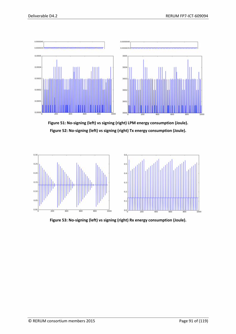
Deliverable D4.2 RERUM FP7-ICT-609094
Figure 51: No-signing (left) vs signing (right) LPM energy consumption (Joule).
Figure 52: No-signing (left) vs signing (right) Tx energy consumption (Joule).
Figure 53: No-signing (left) vs signing (right) Rx energy consumption (Joule).
© RERUM consortium members 2015 Page 91 of (119)

RERUM FP7-ICT-609094 Deliverable D4.2
Figure 54: No-signing (left) vs signing (right) Total energy consumption (Joule).
From the simulation results it becomes clear that the signing process results in extra energy consumption, which may be even five times higher than in the case where no signing is employed. Hence, the trade-off between security and battery lifetime is something that must be considered. For example, it may be required to optimize battery lifetime by adjusting the level of required protection through adequate security policies.
Page 92 of (119) © RERUM consortium members 2015

Deliverable D4.2 RERUM FP7-ICT-609094
6 Low-Power Hardware The RE-Mote design has been broken down into two hardware releases: an earlier one, namely prototype A, with the purpose of gathering an early feedback from involved partners and validate the design towards a more definitive one to be used in the upcoming Use Cases trials, and the release candidate prototype B, which comprises the lessons learned from the previous design, in both hardware implementation and user experience.
The design criteria for the RE-Mote can be summarized into the following:
• Low-Power design, • Support for 2.4 GHz and 868 MHz bands, IEEE 802.15.4 compliant, • Easy to use and integrate into existing products and Smart City applications
The possibility to enable a dual-band operation, featuring a sub-1Ghz transceiver on board, allows to further extend the network coverage and effectively reduce the number of required RD required to cover the same area, thus also minimizing the implementation and installation costs of future Smart City deployments, making the distributed sensor model more appealing to both integrators and city managers.
Many Smart City applications (such as energy metering, lighting control, etc.) nowadays require a low power consumption footprint. Even if the devices are meant to be powered by mains, keeping the energy consumption low ensures a minimum impact on fixed and variable costs, like electricity, making affordable Smart City solutions.
The Low Power design approach has been broken down into two single factors:
• Component selection. • Minimization of current consumption due to design flaws. • Hardware low-power mechanisms.
The component selection seems the most obvious factor upon selecting a component, but it has to be understood as a complete analysis on its current consumption on all possible operation states, such as active mode, idle mode, operation frequency and other characteristics such as the quiescent current draw and the voltage drop-out.
Ignoring the above results into design flaws, in which for example a given component would not work because the required input voltage level doesn’t reach the minimum due to a voltage drop-out. Understanding how the components will interact within an operating block (basically components grouped to provide a feature), and early prototyping these blocks is also part of the low-power design and minimization of design flaws, providing early milestones of current consumption and minimum operation requirements, to allow further iterations to optimize the design. A good example of this is are the RGB LEDs used in the prototype A: when measuring in a bright room the current consumption was 50uA higher than in a dark room, thus indicating the LEDs were actually acting as input photodiodes, then requiring to implement a MOSFET (metal-oxide transistor) to prevent this.
After validating a feature provided by a component block, the design is validated with multiple use cases, to also test the component block interactions with other blocks, for such cases as powering the RD over different power channels, RD operation while the devices are in idle mode, etc.
The following section comprises the above process, from component selection to the test benchmark used to validate the RE-Mote design.
© RERUM consortium members 2015 Page 93 of (119)

RERUM FP7-ICT-609094 Deliverable D4.2
6.1 Low-Power Hardware Design Characteristics
6.1.1 Critical component selection
The components chosen for the design and its criteria selection are summarized below. A more detailed description of the components and its implementation is available in RERUM deliverable D5.2 [RD5.2].
6.1.1.1 Texas Instruments CC2538 system on chip (SoC)
The 32MHz CC2538SF53 ARM Cortex-M3 has been chosen due to its trade-off between processing power and low-power consumption.
The CC2538 has different power operation modes, depending on the available clock sources and peripherals available in each mode. Figure 55 provides a profile of the device operation states at any given time.
Figure 55: CC2538 power consumption characteristics (Source: [TI13a]).
The power management on the CC2538 enables operational power modes, governed by three power saving actions:
• Clock gating of unused or not required peripheral clocks, • Power down of clock sources, • Power supply control
Depending on the configuration register values and the operational mode initiator (the Wait For Interrupt instruction, or WFI), these actions define the following operational power modes (PM) and its limitations as listed in Table 9.
Page 94 of (119) © RERUM consortium members 2015

Deliverable D4.2 RERUM FP7-ICT-609094
Table 9: CC2538 power states (Source [TI13b]).
State Register setting Action I [mA] Limitation
Active WFI clear. Power supply and 32kHz clock source powered on 7-13 None
Sleep WFI asserted, DEEPSLEEP bit in SYSCTRL set.
Power supply and 32kHz clock source powered on. May wake up from any enabled interrupt source
- CPU in sleep
PM0 WFI asserted, DEEPSLEEP bit in SYSCTRL set. PMCTL = 00.
Power supply and 32kHz clock source powered on. May wake up from any enabled interrupt source
- CPU in deep sleep
PM1 WFI asserted, DEEPSLEEP bit in SYSCTRL set. PMCTL = 01
System clock sources powered down, power supply powered on. 32kHz clock source powered on. May wake up from - Pin interrupts - Sleep Mode timer - USB resume
0.6 CPU in deep sleep, all peripherals inactive
PM2 WFI asserted, DEEPSLEEP bit in SYSCTRL set. PMCTL = 10
System clock sources and powered down. 32kHz clock source powered on. May wake up from - Pin interrupts - Sleep Mode timer
0.0013 CPU in deep sleep (inactive), all peripherals inactive
PM3 WFI asserted, DEEPSLEEP bit in SYSCTRL set. PMCTL = 11
System clock sources, power supply and 32kHz clock source powered down. Wake up from pin interrupts only.
0.0004 CPU in deep sleep (inactive), all peripherals and sleep timer inactive
The low-power modes with retention enable quick start-up from sleep and minimum energy spent to perform periodic tasks, however for PM3 it is required to reconfigure previously used peripherals, which should be taken into account for both the sequencing routine as the exit time from that state (136us approx.).
The WFI instruction can be asserted in order to enter PM1, PM2 or PM3 at any point in time and the chip will eventually enter the requested power mode, however as noted in [Figure 56], the transition from Active mode to PM1, PM2 or PM3 should be done on the 16 MHz system clock source. Switching to 16MHz is automatically done by the chip when WDI is asserted, but to better handle the transition timing from states it is recommended to assert WFI while running on 16MHz clock source.
6.1.1.2 Texas Instruments CC1120/CC1200 sub-1Ghz radio frequency transceiver
To enable support for the 868 MHz frequency band (CEPT regulated), the Texas Instruments CC1200 RF transceiver was ultimately chosen over the CC1120 used for the RE-Mote prototype A. Although the differences are obvious regarding the CC1200 performance and features (wideband application support with data rates up to 1MBps, 3dB extra link budget, etc.), regarding power consumption and current draw are not so obvious. [Table 10] compares the transceiver power states.
The first noticeable difference is the radio transmission in High-performance mode (HPM), which is higher for the CC1120, but even if working in the Low Power Mode (LPM) on the CC1120, the limitation of the 200kbps data rate vs the 1Mbps (HPM) and 600kbps (LPM) available in the CC1200 is there, and
© RERUM consortium members 2015 Page 95 of (119)

RERUM FP7-ICT-609094 Deliverable D4.2
making a rule of thumb for which having to spend three times less time transmitting a packet at 33mA in overall would be more efficient.
Figure 56: Power mode transitions (Source: [TI13b]).
Table 10: CC1120/CC1200 power consumption (Source [CC1120] [CC1200]).
State CC1120 CC1200
Power down (with retention) 0.5uA 0.12uA
XOFF 170uA 180uA
IDLE 1.3mA 1.5mA
TX current consumption +10dBm (HPM/LPM) 45/32mA 36/33.6mA
RX Wait for sync (at 38.4kbps) 13.4mA (4-byte preamble)
3.4mA (12-byte preamble)
RX peak current (HPM/LPM) 22/17mA 23.25/19mA
One criterion worth mentioning is the RX current draw upon sniffing for incoming packets, even for a 12-byte preamble length the consumption of the CC1200 is smaller than the CC1120 waiting 4-bytes preambles. As the objective ultimately is to drive the radio stack with a duty-cycling mechanism to save power, this key point makes the CC1200 selection an obvious choice.
In the first Prototype A iteration, the CC1120 was powered ON/OFF by an external co-processor managing the peripherals, requiring an Inter-Integrated Circuit (I2C) command to enable the CC1120 and Micro-SD, but this has been deprecated for the CC1200 in the new Prototype B, and now the CC1200 has an independent input power pin, so the user can decide to power the CC1200 or not if not using the Sub-1Ghz interface. More details about this in the upcoming sections.
Page 96 of (119) © RERUM consortium members 2015

Deliverable D4.2 RERUM FP7-ICT-609094
6.1.1.3 Micro-SD support
The external storage decision was pondered upon 2 choices: on-board flash storage chip or support for external micro-SD cards, both over Serial Parallel Interface (SPI).
As pointed out in the Figure 55, SPI operations takes up to 300uA plus the consumption on Active mode, so the only factors left to ponder are the writing/reading speed and operation, current draw, and features.
As expected the power consumption of the Micro-SD cards is higher than the flash modules (see Figure 55 and Figure 57), however note that typically Micro-SD cards tend to draw 30mA/second approx., but still consumes more power than the flash modules.
Figure 57: SanDisk Micro-SD power requirements (averaged per second) (Source [SMSD]).
Figure 58: Micron M25P16 external flash memory (Source [MIFM]).
As the CC2538 runs on 32 MHz tops and even if there are Micro-SD card models with higher speed modes, as a reference a 25 MHz speed is used as reference. The current draw in overall scales down 2-5 times for the Flash modules, closer to the value of writing to the CC2538 internal flash (see Figure 58).
However from the implementation and the features point-of-view, having support for micro-SD cards is highly desirable. A micro-SD will allow users and deployments an easy way to provision logging and configuration information. One example is to retrieve an application log or to provide the configuration information upon boot for a given device.
As in average the current consumption of the erase/write/read operations of the flash modules are close to the CC2538 built-in flash, and the available flash space for the CC2538 is 512 KB (more than
© RERUM consortium members 2015 Page 97 of (119)

RERUM FP7-ICT-609094 Deliverable D4.2
enough for actual applications), generally speaking the cost of providing 12Mbit (2 MB) extra flash storage is not attractive.
As the sleep/standby current is over 100nA for both options and likely the read/write operations are not expected to happen often, the key goal is to minimize this draw source, then focus on optimizing the Micro-SD operation (storing bulks of data instead of writing constantly, etc.). The Micro-SD slot has a switch (SW1 in Figure 59) that upon inserting a micro-SD it powers on the device, providing also over a second switch (SW2) a readable pin wired to the CC2538, to detect whether the Micro-SD card is present or not. The SW2 switch also allows to power on/off the micro-SD programmatically from the CC2538, by configuring the pin as output and clearing its state. The 1MOhm series resistor limits the current drawn when not used to 33nA.
Figure 59: SD/MMC card schematic RE-Mote prototype B.
As with the CC1120 in the Prototype A, the Micro-SD module was alternatively powered on/off by an external co-processor, but this was deprecated to simplify the RE-Mote operation and design, as noted above the current draw has been greatly minimized.
6.1.1.4 Power management block
To control the power operation of the RE-Mote when powered over USB or external power supply (LiPo battery, solar cell or VDC power supply up to 16V), a battery management module is present in both early through prototype A and now validated in the Prototype B. The BQ24072 [BQ24] allows the RE-Mote to be powered over different power supplies options, charging when powered a connected LiPo battery, suitable for most Smart City applications running on a low-power budget or over solar panels. Table 11 summarizes the battery charger current draw.
Table 11: Battery charger current draw (Source [BQ24]).
Quiescent current Battery 6.5 μA
Quiescent current Sleep 0.2 μA
Quiescent current Active 1.5 mA
The battery manager allows to completely shut down the RE-Mote power supply, being only powered at the time: the Nano Timer [TP5110] (programmable timer with ultra-low power consumption), an I2C-based RTC (real-time clock), and an auxiliary MCU, this serves a double purpose:
Page 98 of (119) © RERUM consortium members 2015

Deliverable D4.2 RERUM FP7-ICT-609094
• Reduce the power consumption of the RE-Mote by powering down the CC2538 and all on-board components, such as the CC1200, Micro-SD, attached sensors and actuators powered by the RE-Mote,
• Allow the RE-Mote to be periodically woken up, either via the Nano Timer (with a configurable time selectable by a resistor value), or by the RTC via an interrupt pin to the auxiliary MCU.
There is a pin wired from the RTC to the CC2538, to allow exiting PM3 mode, effectively providing another power optimization method, one able to retain RAM.
The auxiliary MCU in the Power management block is the 8-bit PIC 12F635 [PIC12F], chosen due its ultra-low power implementation with 8.5uA in active mode (32 kHz operation frequency) and 1nA in standby mode. The Nano Timer is a power gating module with current consumption of 35nA, and allows periodic shutdown periods of 100ms up to two hours (depending on the resistor value connected). In conjunction with the battery manager, the low-power RTC and the CC2538, the Nano Timer can allow overall power savings by periodically wake-up the application, execute and go back to shutdown mode. This differs from a regular sleep mode as practically all on-board components are off.
The former RE-Mote prototype A featured an ATtiny 1634 [AT1634] driven over I2C by the CC2538, exposing an Application Programming Interface (API) to power on/off connected peripherals, the Micro-SD module and the CC1120. The ATtiny was also able to act as a Timer and gate down the battery manager, enter sleep mode and resume the operation after being woke up by its internal watchdog timer (WDT).
This implementation however proved to be cumbersome and only got the current consumption down to 5uA (ATtiny1643 plus others), which is more than the current goal of a few hundred nA’s, as shown in Table 12.
Table 12: Prototype A and B power management consumption (overall).
State ATtiny1634 [AT1634]
(1MHz)
Battery manager [BQ24]
Nano Timer [TP5110]
MCU (1MHz) [PIC12F]
Active Mode 400uA
6.5uA 35nA
140uA
Idle Mode 80uA 200nA
Power Down (WDT On) 2uA 1.5uA
We cut the dependency of the Battery manager in shutdown mode for the Prototype B and power directly from the Nano Timer, saving 4.5-6.5uA in average due to the battery manager quiescent current, running our wake-up timer to exit shutdown mode off the Nano Timer, reducing this feature to 35nA instead of the 2uA average of the ATtiny1634 with the WDT enabled.
In practice the CC2538 interfaces to the MCU consumption manager via 1-Wire interface (routed also externally to a non-mounted button to manually drive the command sequences), indicating the power manager block to enable or disable the Nano Timer. From this point the Nano Timer is then in charge of the power control sequence and states.
The MCU [PIC12F] can also be awaken once in Idle Mode by an interrupt from the RTC module, effectively allowing the entire system to be clocked off the WDT. The Nano Timer once enabled will periodically put the system in shutdown mode, depending on the value of R47 (DELAY input pin), the shutdown period may vary between 100ms and 2 hours. The CC2538 over the DONE pin can choose to enter shutdown mode before the expiration of the shutdown timer by sending a 100ns pulse to the Nano Timer. The Nano Timer implementation is shown in Figure 61.
© RERUM consortium members 2015 Page 99 of (119)

RERUM FP7-ICT-609094 Deliverable D4.2
Figure 60: PIC12F635 Shutdown enable MCU.
Figure 61: Nano Timer implementation.
6.1.1.5 Programming block
Besides programming the CC2538 over JTAG, the internal bootloader allows the device to be programmed over serial, but only if the flash memory is blank or the bootloader backdoor is enabled (CCA are in flash), requiring to pull a PAx pin low during boot.
In the Prototype A, an FTDI [FT22] chip was using to convert from serial to USB and provide a micro-USB port to connect over cable, this provided 2 Universal Asynchronous Receiver Transmitter (UART) channels [0-1] to the host, from which channel 1 was used for programming and debugging (printing console output to the host). Upon programming, the TX/RX lines activity were detected and routed to the CC2538 PA3 pin to manually enable the sequence that unlocks the bootloader. The PA3 pin was also routed as the user button along with a user button, to enable entering the bootloader sequence manually upon programming the device.
Table 13: CP2104 [CP2104] vs FTDI [FT22] current draw.
State FTDI [FT22] CP2104 [CP2104] PIC12F519 [PICBL]
Active Mode 70 mA 17mA 0.25mA
Page 100 of (119) © RERUM consortium members 2015

Deliverable D4.2 RERUM FP7-ICT-609094
Idle Mode 500uA 100uA 9uA
For the Prototype B, the bootloader sequence is now executed by an auxiliary PIC12F519 MCU [PICBL] and the CP2104 [CP2104], as the FTDI was discarded due to the following reasons:
• Bigger footprint than the CP2104 (4x bigger), • Over-heated when connected over USB, • More expensive than the CP2104, • Having 2 channels on-board was not required as one channel for programming and debugging
was enough
Even if the Prototype A was capable of unlocking its bootloader and be programmed over USB without having to manually input the bootloader sequence, due to the RESET/PA3 commute, the CC2538 was being restarted when connecting over the USB to debug, which was cumbersome depending on the application you are currently debugging. Using an additional MCU [PICBL] allowed to trigger the BSL sequence and to log the console output without interrupting of affecting the CC2538 operation.
The current consumption for the programming module is not under consideration, as it is assumed the block will be powered over USB. While connected over USB, the current should be less than 500mA, as the maximum allowed by USB 2.0 compliant devices [USBP]. To enforce this current limitation, we have selected the CP2104 and its auxiliary MCU with low-power design in mind (see Table 13 for comparison).
6.2 Contiki’s Low-Power Module The Contiki CC2538 low-power mode (LPM) module takes advantage of the chip’s low power characteristics. The LPM module supports automatic switching between active, sleep and PM0, PM1 and PM2 depending on combined information about the state of the operating system, the device and all relevant peripherals.
The LPM module can be configured at compile time with the following configuration options:
• LPM_CONF_ENABLE: Can be used to disable the module altogether, • LPM_CONF_MAX_PM: Can set the maximum supported PM. In this context, maximum
corresponds to the PM number. Therefore a high PM means lower power consumption, • LPM_CONF_STATS: Can be used to enabled/disable LPM-related statistics.
The LPM module currently does not support PM3, which puts the device in a state whereby it can only be woken up by a GPIO event (e.g. button press). Conceptually, this corresponds to a full device shutdown.
The default configuration for the RE-Mote Contiki platform is listed in the snippet (Snippet 1). We can see that default configuration enables the module, allows the maximum possible PM and disables stats in order to reduce RAM overhead.
© RERUM consortium members 2015 Page 101 of (119)

RERUM FP7-ICT-609094 Deliverable D4.2
Snippet 1: Default LPM Configuration.
6.2.1 LPM logic
As part of Contiki’s port for the RE-Mote platform, after the device boots it enters a very simple while loop that runs forever. This is listed in Snippet 2 and is identical to the one used by Contiki’s CC2538DK port that also uses the same chip.
Snippet 2: Contiki's Port for the RE-Mote: The Main Loop.
This main loop first handles all operating system events, refreshing the watchdog timer (WDT) between events to prevent a WDT trigger. Once all events have been handled, the LPM module is invoked in order to enter a low-power state. The lpm_enter() routine automatically selects the most suitable power state based on a set of criteria:
• User configuration, • Chip and peripheral state, • Anticipated sleep duration
/** * \name LPM configuration * @ */ #ifndef LPM_CONF_ENABLE #define LPM_CONF_ENABLE 1 #endif /** * \brief Maximum PM * * The SoC will never drop to a Power Mode deeper than the one specified here. * 0 for PM0, 1 for PM1 and 2 for PM2 */ #ifndef LPM_CONF_MAX_PM #define LPM_CONF_MAX_PM 2 #endif #ifndef LPM_CONF_STATS #define LPM_CONF_STATS 0 #endif /** @ */
while(1) uint8_t r; do /* Reset watchdog and handle polls and events */ watchdog_periodic(); r = process_run(); while(r > 0); /* We have serviced pending events. Enter a Low-Power mode. */ lpm_enter();
Page 102 of (119) © RERUM consortium members 2015

Deliverable D4.2 RERUM FP7-ICT-609094
User configuration always takes precedence: For instance, the LPM module will never select PM2 if the user has specified that the maximum allowed PM is PM1.
Code modules that are affected by LPM operation (e.g. peripheral drivers) can register themselves with the LPM module by calling the lpm_register_peripheral() function. Within lpm_enter(), the LPM module will query all registered modules in order to ask for permission to drop to PM1 or PM2. If any of the modules disallows PM1+, the chip will drop to PM0 instead. A typical reason why a module would want to disallow PM1+ is because entering this PM would disrupt the peripheral’s operation. For example, if the SPI or UART were busy, entering PM1 or PM2 would interrupt the operation abruptly.
In a nutshell, the LPM module will select PM1 or PM2 if:
• All registered modules allow it and, • The Sleep Timer is scheduled to fire an interrupt in the future (this guarantees that the chip
can wake up from deep sleep) and, • The radio is off and, • The USB Phase-Locked Loop (PLL) is off (therefore the USB controller is not active) and, • The anticipated sleep duration is sufficiently long to justify the temporal overhead incurred by
entering deep sleep and waking up.
If any of the above does not hold true, the chip will either simply sleep or enter PM0 instead. In both cases, any interrupt will bring the chip out of sleep / deep sleep respectively. In the best-case scenario, the chip will sleep or deep-sleep for a maximum of 7.8125ms, which is the interval between two consecutive interrupt-generating clock ticks.
The lpm_enter() routine will also switch the system clock source to the 16MHz oscillator, turning off the more energy-hungry 32MHz Crystal Oscillator (XOSC). When the chip wakes up, the LPM module will automatically power the 32MHz XOSC, which is required for radio operation.
6.3 RE-Mote Contiki power consumption measurements
6.3.1 RE-Mote current consumption benchmark with RIME
To measure the RE-Mote current consumption the remote-demo and cc1120-demo at the examples folder were used. Both example applications basically open a broadcast channel and initialize a periodic event timer, at each expiration reading the sensor values and sending a broadcast message at a given rate. A resumed example is shown in Figure 62.
Upon receiving a broadcast the RE-Mote blinks a LED and prints the message content. In the prototype A the TMP102 [TMP102] temperature sensor is also tested.
Typically the highest current draw in any radio-dependant device is the radio itself, in the case of the RE-Mote (as shown in sections before) the 2.4 GHz and Sub-Ghz RF transceivers are the main power consumption devices. As of the date of writing this document, there is no support in Contiki to use two RF interfaces at the same time, so only one can be used at a given time, both governed by ContikiMAC [D11] or with no duty-cycle mechanism (NullRDC), leaving the radio on for the remainder of the application. Figure 63 shows the default RDC settings.
A first benchmark of the RE-Mote Prototype A power consumption is shown in Figure 64.
When using NullRDC the radio is permanently on (unless powered off by the application, but no mechanism is used to further manage it), so even if the CC2538 goes to sleep the main contributor to the current draw is the RF module. As shown in Figure 64, the CC1120 has a higher current consumption as expected due to adding its own consumption to the CC2538, while the graph showing
© RERUM consortium members 2015 Page 103 of (119)

RERUM FP7-ICT-609094 Deliverable D4.2
the CC2538 operating with the 2.4GH RF interface (namely remote-demo) had the CC1120 shutdown via the co-processor.
Figure 62: RE-Mote test code example.
Figure 63: Radio Duty cycle settings from RE-Mote’s contiki-conf.h header.
From Figure 64 is clear the power savings due to ContikiMAC operation (8 Hz channel check), namely more than 50% reduction while also highly available to others devices in the network, as expected for cases such as a sleepy router or forwarder node in a mesh network. However 15mA average still scales quite high for most applications.
Using the shutdown mode, as explained in the Power management section earlier in this chapter, significantly dropped the current draw to few mill amperes, as the RE-Mote was kept powered off and the only devices operating were the co-processor and the battery charger (as depicted in Table 11), only awakening the CC2538 and CC1120 after a given period (for this test up to a minute period).
The shutdown mode test results are shown in Figure 65.
Comparing back to back the results of Figure 64 for the remote-demo running with ContikiMAC, the average current consumption of 61 scenario for a broadcasting period of 1 minute is approximately 10 mA, assuming the radio is ON for just 35ms while it senses the channel and transmits, and the remainder of the time the radio is duty-cycling drawing approximately 10 mA, which is however higher than the 190uA featured in Figure 65.
Page 104 of (119) © RERUM consortium members 2015

Deliverable D4.2 RERUM FP7-ICT-609094
Figure 64: RE-Mote current consumption (2.4 GHz and Sub-Ghz) with different MAC settings.
Figure 65: RE-Mote current consumption in shutdown mode with remote-demo.
A close-up look at the shutdown mode current consumption is taken at Figure 66, the average is 4.47 uA, which relatively close to the 6.7 uA expected from the battery manager [BQ24] and the ATtiny [AT1634] with the WDT running as pointed out in Table 12. From the values in Figure 66 the ticking WDT of the ATtiny is shown as an oscillating current draw that could be further minimized if using a different MCU running in tick-less mode.
However upon testing the RE-Mote’s Prototype B shutdown mode, with the RTC and Nano Timer running, and the PIC [PIC12F] in sleep mode, there is an improvement of 13x, being the average current draw 327nA as shown in Figure 67, from which 34.3nA are from the Nano Timer, 66.6nA from the RTC, and 226.7nA from the PIC.
One caveat of the shutdown mode however is the RE-Mote having to boot again each time is powered back on by the ATtiny (prototype A) or the Nano-Timer (prototype B), but for applications that doesn’t require to retain a given state or information, this operation mode is suitable to keep the power
© RERUM consortium members 2015 Page 105 of (119)

RERUM FP7-ICT-609094 Deliverable D4.2
footprint low. Alternatively there is also the option of storing variables and information (such as routing if the deployment is a rather static one) in the internal flash memory or the Micro-SD before going into shutdown mode.
Figure 66: RE-Mote current consumption in shutdown mode (close-up).
Figure 67: RE-Mote Prototype B shutdown mode current draw (piled)
The CC2538 is able to retain 16KB of RAM memory of its 32 KB RAM total while in PM2 and PM3, alternatively one could use the RTC and put the device to sleep, using the RTC interrupt pin to awake the CC2538 out of PM3 state. As the RE-Mote is aware of time and date due to the on-board RTC, schemes like having coordinate wake-up times to rebuild certain mesh routes towards the Border Router are enabled by the RE-Mote.
6.3.2 RE-Mote current consumption benchmark with IPv6 and HTTP posts to Ubidots
A real-life example was used to measure the RE-Mote power consumption, while posting HTTP messages over IPv6. This the most critical case scenario as HTTP/TCP transactions require a higher packet exchange, than non-connection-oriented protocols such as CoAP.
Page 106 of (119) © RERUM consortium members 2015

Deliverable D4.2 RERUM FP7-ICT-609094
Ubidots [UBIDT] is an IoT platform to capture and display data in real time and over a wide variety of widgets and options, featuring a RESTful API with IPv4 and IPv6 endpoints to connect devices to the platform. The tests were done using the Ubidots example and application from [GUBI], ContikiMAC as MAC driver with a channel check period of 8 Hz, and a publishing period of 1 minute, that is, the RE-Mote exits shutdown mode every minute, establish a TCP connection and posts to Ubidots. The results are shown in Figure 68, for which the peak current was up to 40 mA approx. and while awake the drawn current oscillates around 10 mA (as also shown in Figure 64) with the lowest values close to 4 mA. In average this scenario yields an average of 2.6 mA which is still significantly lower than the ones depicted in Figure 64, with a real-case example on a Smart Object posting to an IoT platform over IPv6.
As the shutdown current is around 4.47 uA as shown in Figure 66, the Nano Timer and power management block improvements done for the RE-Mote’s Prototype B would greatly decrease this as shown in Figure 67.
Figure 68: RE-Motes current draw posting to Ubidots (IPv6/HTTP).
In Figure 69 and Figure 70 the timings and frames exchanged during a single posting operation are shown, which helped to understand and verify the example. Further optimizations were possible to perform for this scenario, to improve the timings and reduce the radio activity to decrease power, but we favoured the worst-case scenario implementation, as our aim was to establish a benchmark to validate the design, and provide an overview of the example with metrics to improve in future works.
Figure 69: RE-Mote’s Ubidots application’s timing.
© RERUM consortium members 2015 Page 107 of (119)

RERUM FP7-ICT-609094 Deliverable D4.2
Figure 70: Wireshark captures of IPv6 traffic in RE-Mote’s Ubidots application.
The results of posting to Ubidots are shown below in Figure 71, validating the end-to-end IPv6 energy consumption test.
Figure 71. RE-Mote temperature readings posted to Ubidots.
To better understand these results, let us assume using a LiPo battery of 2500 mAh capacity to have a rough approximation to battery life, without taking into consideration the battery life and using the 100% of its capacity. Without assuming a periodic power supply source to recharge the batteries while operating (like a solar panel), the discharge times are shown in Table 14. These results should not be taken as the best results, but merely as references, as the test scenarios were not optimized to provide an ultra-low power application but rather to validate the shutdown mode design, as extra measures can be taken to reduce the power consumption, like reducing the transmission power (all scenarios are using the highest available), increasing the posting period, etc.
Table 14: Discharge times for different RE-Mote’s scenarios.
Test scenario (1 minute)
NullRDC ContikiMAC With Shutdown (Prototype A)
With Shutdown (Prototype B)
Ubidots example
3.3 days (31.47mA avg)
10.41 days (10mA avg)
39.9 days (2.61mA avg)
48.22 days (2.16mA avg)
RIME scenario 3.3 days (31.47mA avg)
10.41 days (10mA avg)
548 days (0.19mA avg)
3927 days (26.57uA avg)
The calculations (following [TIEB]) to approximate the Shutdown mode values of Prototype B into the Prototype A benchmarks assumed: timing and current draw while in active mode (Radio sending and
Page 108 of (119) © RERUM consortium members 2015

Deliverable D4.2 RERUM FP7-ICT-609094
receiving) to be the same for both, replacing shutdown mode values and period accordingly. This yields for the RIME scenario a 99.94% time in which the RE-Mote is in shutdown mode, being the remainder (approx. 35ms) the time the RE-Mote is broadcasting data, running at 45mA (worst case scenario with no ContikiMAC).
For the Ubidots scenario we approximate the calculations by taking the timing from Figure 69, being the RE-Mote in shutdown mode approx. 72.4% every 1 minute period, being the remainder drawing 10mA in average as ContikiMAC is used.
6.3.3 Comparison with the Zolertia Z1
As a closing note in this section, we present a brief comparison between the RE-Mote and Zolertia’s older platform, the Z1. Table 15 presents an overall comparison between the two platforms. This is further detailed on a per-component basis in Table 16.
Table 15. Zolertia’s Z1 mote and RE-Mote overall comparison
Feature Z1 mote RE-Mote
Minimum operation mode 18 µA (MCU LPM3, others in sleep/off)
350 nA (shutdown mode)
Performance vs consumption 0.625 mA/MHz 0.406 mA/MHz
Size 55 x 33 mm 73.77 x 40.30 mm
Component density 5.5 per cm2 6.84 per cm2
© RERUM consortium members 2015 Page 109 of (119)
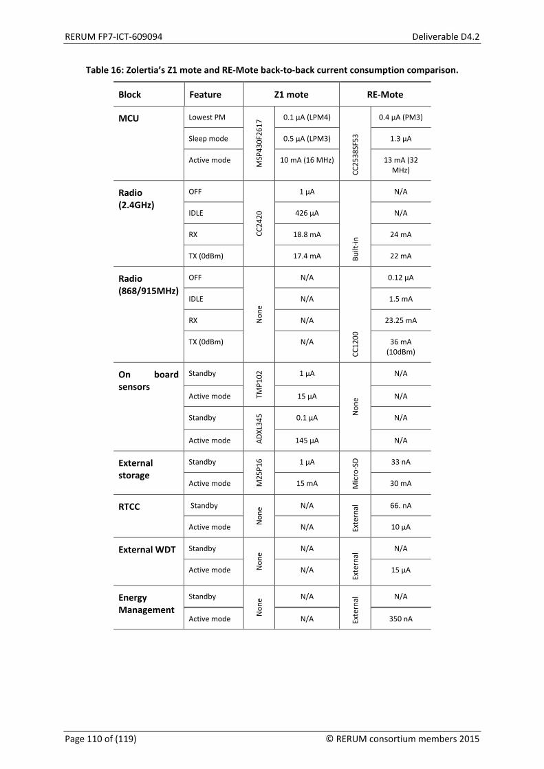
RERUM FP7-ICT-609094 Deliverable D4.2
Table 16: Zolertia’s Z1 mote and RE-Mote back-to-back current consumption comparison.
Block Feature Z1 mote RE-Mote
MCU Lowest PM
MSP
430F
2617
0.1 µA (LPM4)
CC25
38SF
53
0.4 µA (PM3)
Sleep mode 0.5 µA (LPM3) 1.3 µA
Active mode 10 mA (16 MHz) 13 mA (32 MHz)
Radio (2.4GHz)
OFF
CC24
20
1 µA
Built
-in
N/A
IDLE 426 µA N/A
RX 18.8 mA 24 mA
TX (0dBm) 17.4 mA 22 mA
Radio (868/915MHz)
OFF
Non
e
N/A
CC12
00
0.12 µA
IDLE N/A 1.5 mA
RX N/A 23.25 mA
TX (0dBm) N/A 36 mA (10dBm)
On board sensors
Standby
TMP1
02
1 µA
Non
e
N/A
Active mode 15 µA N/A
Standby
ADXL
345 0.1 µA N/A
Active mode 145 µA N/A
External storage
Standby
M25
P16 1 µA
Mic
ro-S
D 33 nA
Active mode 15 mA 30 mA
RTCC Standby
Non
e N/A
Exte
rnal
66. nA
Active mode N/A 10 µA
External WDT Standby
Non
e
N/A
Exte
rnal
N/A
Active mode N/A 15 µA
Energy Management
Standby
Non
e N/A
Exte
rnal
N/A
Active mode N/A 350 nA
Page 110 of (119) © RERUM consortium members 2015

Deliverable D4.2 RERUM FP7-ICT-609094
7 Conclusions This document presented a series of mechanisms aiming to reduce energy consumption of RDs and gateways, aiming to increase the overall lifetime of RERUM deployments. The evaluations undertaken as part of this Task were conducted using analytical methods or simulations. Evaluations on real hardware in a lab environment will be undertaken as part of Task 5.3 and will be documented in a subsequent deliverable.
The key findings of our analysis are summarised as follows:
Minimization of Data Sampling and Transmission using Compressive Sensing: within RERUM the CS techniques has been heavily utilized aiming to exploit its benefits of providing simultaneously encryption and compression, thus achieving security and energy efficiency in one single step. Here, we extended the state of the art by introducing an adaptive scheme aiming to mitigate the problem of unpredicted changes in the sparsity of the signal that result in increase of the reconstruction error. With the approach presented here and tested in extended simulations, we are able to quickly identify signal sparsity changes, and maintain a very low reconstruction error. Finally, with the use of the Matrix Completion technique together with the CS technique we have shown that we can mitigate packet losses, which are very frequent in the wireless sensor network environments.
Congestion-Aware Duty Cycling RDs in 6LoWPANs: Simulation results presented in Section 3.1 show that CADC outperforms other mechanisms in terms of energy usage. Experiments also demonstrated that dynamic MACs maintain lower energy consumption than static MAC configurations. Compared to the default RDC configuration of ContikiMAC, CADC achieved over 50% lower energy consumption in both idle and active network states.
Energy-aware relay properties of RERUM gateways: The results presented in Section 3.2 provide insight about systems of between one and four gateways serving up to 30 RDs in terms of aggregate throughput, average queue size and packet delay. The results reveal that having Full-Duplex gateways switched on half of the time is beneficial when the communication channel is poor.
Energy consumption of multicast forwarding with BMFA: Simulation results show that BMFA decreases the energy consumption of multicast forwarding by 50% or more, depending on configuration. This is due to the total lack of control messages, the lack of retransmissions and also the lower algorithmic complexity.
Adaptive and energy-efficient multi-radio selection mechanisms: Results presented in Section 4.2 indicate that the new adaptive threshold-based SD (t-SD) receiver is adopted as the optimal solution for the trade-off between performance and complexity. Based on the new scheme, it is proved that the complexity of the conventional diversity receivers is reduced, without considerable affecting the performance. Also, based on the versatility of the Nakagami-m fading distribution to model heterogeneity environments, the performance of the t-SD is studied under more realistic wireless environments. It is shown that in many cases t-SD, outperforms SD in terms of the performance and complexity trade-off.
Power consumption evaluation of authorization mechanisms: The Hash Token mechanism developed as part of RERUM outperforms other schemes in terms of processing energy, as well as in terms of code size by a large margin. Compared to Kerberos (AES), the energy efficiency decrease is marginal (from 0.56mWs to 0.53mWs), but code size decreases by approximately 30 times.
Energy consumption of the JSON Signature Scheme: From the simulation results presented in Section 5.2 it becomes clear that the signing process used by JSS results in extra energy consumption, which may be even five times higher than in the case where no signing is employed. Hence, the trade-off between security and battery lifetime is something that must be considered. For example, it may be required to optimize battery lifetime by adjusting the level of required protection through adequate security policies.
© RERUM consortium members 2015 Page 111 of (119)

RERUM FP7-ICT-609094 Deliverable D4.2
Low-Power Hardware: Measurements indicate that, when using a firmware that minimises the transmission of control and data packets, the power consumption of the RE-Mote’s second prototype is approximately five times lower than that exhibited by the first prototype. The average consumption when the device’s shutdown capability is in use has dropped from approximately 200uAs to less than 30uAs. This decrease is attributed to intelligent software, but more importantly on the big design improvements between the two versions, with the second one using ultra low-power hardware components.
Page 112 of (119) © RERUM consortium members 2015

Deliverable D4.2 RERUM FP7-ICT-609094
References [AFRA+13] M. Abbas, H. Fazirulhisyam, S. Raja, A. Azmir Raja, A. Borhanuddin Mohd, O. Mohamed,
K. Sabira, “Multicast-Unicast Data Delivery Method in Wireless IPv6 Networks”, Journal of Network and Systems Management, February 2013
[AKK05] K. Akkaya et al., “A survey on routing protocols for wireless sensor networks”, Elsevier Ad Hoc Networks, pp. 325-349, 2005.
[ALH12] O. El Ayach, A. Lozano, and R. W. Heath, “On the overhead of interference alignment: Training, feedback, and cooperation,” IEEE Trans. Wireless Commun., vol. 11, no. 11, pp. 4192–4203, Nov. 2012.
[APA15] I. Avgouleas, N. Pappas, and V. Angelakis. “Cooperative Wireless Networking with Probabilistic On/Off Relaying,” IEEE Vehicular Telecommunications Conference 2015 – Spring (VTC2015-Spring), Workshop on Heterogeneous Networking for the Internet of Things, Glasgow, UK, May 2015.
[AS72] M. Abramowitz and I. A. Stegun, Handbook of Mathematical Functions, with Formulas, Graphs, and Mathematical Tables, 9th ed. New York: Dover, 1972.
[AT1634] ATMEL ATtiny 1634 “8-bit Atmel tinyAVR Microcontroller with 16K Bytes In-System Programmable Flash”, Atmel-8303H-AVR-ATtiny1634-Datasheet, 2014.
[AWBD10] M. Anwander, G. Wagenknecht, T. Braun, and K. Dolfus, “BEAM: A burst-aware energy-efficient adaptive mac protocol for wireless sensor networks,” in Networked Sensing Systems (INSS), 2010 Seventh International Conference on Network Sensing Systems, June 2010, pp. 195 –202.
[B++11] P. Boufounos et al., “Sparse signal reconstruction from noisy compressive measurements using cross validation,” in IEEE/SP SSP’07. IEEE, 2007, pp. 299–303.
[BHRW+07] W. Bajwa, J. Haupt, G. Raz, S. Wright, and R. Nowak, “Toeplitz structured compressed sensing matrices,” in Proc. of SSP, 2007, pp. 295–298.
[BLMS+14] A. Lioumpas, T. Mouroutis, “Hybrid Threshold-Based Selection Diversity Receivers for Efficient Resources Utilization”, International Workshop on Computer-Aided Modeling Analysis and Design of Communication Links and Networks (CAMAD), 2014
[BNCK10] G. J. Bhaumik S., Narlikar, S. Chattopadhyay, and S. Kanugovi, “Breathe to stay cool: adjusting cell sizes to reduce energy consumption,” in 1st ACM SIGCOMM Workshop on Green Networking, pp. 41–46, 2010.
[BR14] P. S. Bithas and A. A. Rontogiannis, “Analysis of threshold-based selection diversity receivers,” in IEEE Vehicular Technology Conference, Sep. 2014.
[BRR08] E. Basha, S. Ravela, and D. Rus, “Model-based monitoring for early warning flood detection,” in Proc. of SenSys, 2008, pp. 295–308.
[BQ24] Texas Instruments, “bq2407x 1.5-A USB-Friendly Li-Ion Battery Charger and Power-Path Management IC”, SLUS810K, 2015.
[BY13] H. Byun and J. Yu, “Adaptive duty cycle control with queue management in wireless sensor networks,” IEEE Transactions on Mobile Computing, June 2013.
[BYAH06] M. Buettner, G. Yee, E. Anderson, and R. Han, “X-MAC: a short preamble mac protocol for duty-cycled wireless sensor networks,” in Proceedings of the 4th international conference on Embedded networked sensor systems, ser. SenSys ’06. New York, NY, USA, ACM, 2006, pp. 307–320.
© RERUM consortium members 2015 Page 113 of (119)
RERUM FP7-ICT-609094 Deliverable D4.2
[CC1120] Texas Instruments, “High Performance RF Transceiver for Narrowband Systems", SWRS112H, 2015.
[CC1200] Texas Instruments, “CC1200 Low-Power, High Performance RF Transceiver", SWRS123D, 2014.
[CFT15] P. Charalampidis, A. Fragkiadakis, E. Tragos, "Rate-adaptive compressive sensing for IoT applications", VTC2015-Spring, May 2015, Glasgow, UK.
[CH10] T. Clausen and U. Herberg, “Intelligent sensors, sensor networks and information processing (ISSNIP), 2010 sixth international conference on,” 2010, pp. 7–12.
[CP10] E. Candes and Y. Plan, “Matrix completion with noise,” Proceedings of the IEEE, vol. 98, no. 6, pp. 925–936, 2010
[CRH09] C. T. Chou, R. Rana, W. Hu, “Energy efficient information collection in wireless sensor networks using adaptive compressive sensing,” Local Computer Networks, 2009. LCN 2009. IEEE 34th Conference on, 2009.
[CW08] E. Candes and M. Wakin, “An introduction to compressive sampling,” IEEE Signal Processing Magazine, vol. 25, no. 2, pp. 21–30, 2008.
[CW11] W. Chen and I. Wassell, “Energy efficient signal acquisition via compressive sensing in wireless sensor networks,” in Proc. of ISWPC, 2011.
[CYL08] H. Chen, G. Yao, and H. Liu, “Traffic adaptive duty cycle mac protocol for wireless sensor networks,” in Wireless Communications, Networking and Mobile Computing, 2008. WiCOM ’08. 4th International Conference on, Oct. 2008, pp. 1 –4.
[D06] D. Donoho, “Compressed sensing,” IEEE Transactions on Information Theory, vol. 52, pp. 1289–1306, 2006.
[D10] D. Donoho and J. Tanner, “Precise undersampling theorems,” Proceedings of the IEEE, vol. 98, no. 6, pp. 913–924, June 2010.
[D11] A. Dunkels, “The ContikiMAC Radio Duty Cycling Protocol”, Tech. Rep. T2011:13, Swedish Institute of Computer Science, 2011
[DEFT11] A, Dunkels, J. Eriksson, N. Finne, and N. Tsiftes. Powertrace: Network-level power profiling for low-power wireless networks, 2011
[DGNT12] T. Do, L. Gan, N. Nguyen, and T. Tran, “Fast and efficient compressive sensing using structurally random matrices,” Signal Processing, IEEE Transactions on, vol. 60, no. 1, pp. 139–154, Jan 2012.
[DL03] T. van Damand, K. Langendoen, “An adaptive energy-efficient MAC protocol for wireless sensor networks,” in Proceedings of the 1st international conference on Embedded networked sensorsystems,ser.SenSys’03. New York, NY, USA, ACM, 2003, pp. 171–180.
[DOTH07a] A. Dunkels, F. Österlind, N. Tsiftes, Z. He, Z. “Demo abstract: Software-based sensor node energy estimation”, In: Proc. Fifth ACM Conference on Networked Embedded Sensor Systems (SenSys 2007), Sydney, Australia, 2007
[DOTH07b] A. Dunkels, F. Österlind, N. Tsiftes, Z. He, Z “Software-based on-line energy estimation for sensor nodes”, In: Proc. Fourth Workshop on Embedded Networked Sensors (Emnets IV). Cork, Ireland, 2007
[FAT13a] A. Fragkiadakis, I. Askoxylakis, and E. Tragos, “Secure and energy efficient life-logging in wireless pervasive environments,” in Proc. of the 1st International Conference on Human Aspects of Information Security, Privacy and Trust, 2013.
Page 114 of (119) © RERUM consortium members 2015

Deliverable D4.2 RERUM FP7-ICT-609094
[FAT13b] A. Fragkiadakis, I. Askoxylakis, and E. Tragos, “Joint compressed sensing and matrix-completion for efficient data collection in wsns,” in Proc. of Camad, 2013, pp. 84–88.
[FCT14] A. Fragkiadakis, P. Charalampidis, E. Tragos, "Adaptive compressive sensing for energy efficient smart objects in IoT applications", IEEE Wireless Vitae 2014, Aalborg, Denmark, May 2014.
[FTPC14] A. Fragkiadakis, E. Tragos, S. Papadakis, P. Charalampidis, "Experiences with deploying Compressive Sensing and Matrix Completion techniques in IoT devices", IEEE CAMAD 2014, Athens, Dec. 2014
[FIPS01] National Institute of Standards and Technology (NIST). Advanced Encryption Standard (AES). FIPS Publication 197,2001.
[FNT12] A. Fragkiadakis, S. Nikitaki, and P. Tsakalides, “Physical-layer intrusion detection for wireless networks using compressed sensing,” in Proc. Of WiMob, 2012, pp. 845–852. [GR00] I. S. Gradshteyn and I. M. Ryzhik, Table of Integrals, Series, and Products, 6th ed. New York: Academic Press, 2000.
[HBRN08] J. Haupt, W. Bajwa, M. Rabbat, and R. Nowak, “Compressed sensing for networked data,” Signal Processing Magazine, IEEE, vol. 25, no. 2, pp. 92–101, March 2008.
[HK14] J. Hui, R. Kelsey, “Multicast Protocol for Low power and Lossy Networks (MPL)”, draft-ietf-roll-trickle-mcast-11, Nov. 2014
[HM01] Hazewinkel, Michiel, ed. (2001), "Kolmogorov–Smirnov test", Encyclopedia of Mathematics, Springer, ISBN 978-1-55608-010-4
[HTK08] I. Hakala, M. Tikkakoski, and I. Kivela, “Wireless sensor network in environmental monitoring - case foxhouse,” in Proc. of SENSORCOMM,2008, pp. 202–208.
[IEEE06] Institute of Electrical and Electronics Engineers: "Wireless Medium Access Control (MAC) and Physical Layer (PHY) Specifications for Low-Rate Wireless Personal Area Networks (WPANs)", IEEE Std 802.15.4-2006, 2006
[JKSK+13] N. Javaid, N. Khan, M. Shakir, M. Khan, S. Bouk, and Z. Khan, “Ubiquitous healthcare in wireless body area networks - a survey,” CoRR, vol. abs/1303.2062, 2013.
[JLHK07] J. Jeon, J. W. Lee, J. Y. Ha, and W. H. Kwon, “DCA: Duty-cycle adaptation algorithm for IEEE 802.15.4 beacon-enabled networks,” in Vehicular Technology Conference, 2007. VTC2007-Spring. IEEE 65th, April 2007, pp. 110 –113.
[K+07] P. Karamolegkos et al., “User - profile based communities assessment using clustering methods,” in 18th IEEE PIMRC 2007, Sept 2007, pp. 1–6.
[KD13] L. Keliher and A. Delaney, “Cryptanalysis of the toorani-falahati hill ciphers,” IACR Cryptology ePrint Archive, 2013.
[L62] R. Loynes, “The stability of a queue with non-independent inter-arrival and service times,” Proc. Camb. Philos.Soc, vol. 58, no. 3, pp. 497–520, 1962.
[LBA13] A. Lioumpas, P. Bithas, and A. Alexiou, “Partitioning of distributed MIMO systems based on overhead considerations,” IEEE Wireless Commun. Lett., vol. 2, no. 6, pp. 579–582, Dec. 2013.
[LCHG11] P. Levis, T. Clausen, J. Hui, O. Gnawali, J. Ko, J, “The trickle algorithm”, RFC 6206, March 2011.
[LKT08] A. S. Lioumpas, G. K. Karagiannidis, and T. A. Tsiftsis, “Adaptive generalized selection combining (A-GSC) receivers,” IEEE Trans. Wireless Commun., vol. 7, no. 12, pp. 5214–5219, Dec. 2008.
© RERUM consortium members 2015 Page 115 of (119)

RERUM FP7-ICT-609094 Deliverable D4.2
[LLQ10] Liu et al., “A New Adaptive Compressed Sensing Algorithm for Wireless Sensor Networks”, in Proc. of ICSP, pp. 2452-2455, 2010.
[LP++09] S. Lee et al., “Compressed Sensing and Routing in Multi-Hop Networks”, Technical Report, University of Southern California, 2009.
[LPCS04] P. Levis, N. Patel, D. Culler, S. Shenker, “Trickle: A self-regulating algorithm for code propagation and maintenance in wireless sensor networks”, In Proceedings of the first USENIX/ACM sym posium on 15–28), 2004.
[LPS+09] S. Lee et al., “Spatially-localized compressed sensing and routing in multi-hop sensor networks”, in Proc. of GSN, 2009.
[LWSC09] C. Luo, F. Wu, J. Sun, C.W. Chen “Compressive data gathering for large-scale wireless sensor networks.” ACM MOBICOM, 2009.
[M+07] C. Mensing et al., “Location determination using in-band signaling formobility management in future networks,” in 18th IEEE PIMRC 2007, Sept 2007, pp. 1–5.
[M+09] R. Masiero et al., “Data acquisition through joint compressive sensing and principal component analysis,” in IEEE GLOBECOM, 2009.
[MGOP11] V. Michopoulos, L. Guan, G. Oikonomou, and I. Phillips, “A Comparative Study of Congestion Control Algo- rithms in IPv6 Wireless Sensor Networks,” in Proc. 2011 International Conference on Distributed Computing in Sensor Systems and Workshops (DCOSS), Barcelona, Spain, Jun. 2011.
[MGOP12] V. Michopoulos, L. Guan, G. Oikonomou, and I. Phillips, “DCCC6: Duty Cycle-Aware Congestion Control for 6LoW- PAN Networks,” in Proc. 8th IEEE International Workshop on Sensor Networks and Systems for Pervasive Computing (PerSeNS 2012). Lugano, Switzerland: ieee, March 2012.
[MIFM] Micron: “Micron M25P16 Serial Flash Embedded Memory” [Online] Available: http://www.micron.com
[MKHC07] G. Montenegro, N. Kushalnagar, J. W. Hui, and D. E. Culler: “Transmission of IPv6 packets over IEEE 802.15.4 networks,” RFC 4944, Sep. 2007.
[MOPG14] V. Michopoulos, G. Oikonomou, I. Phillips, L. Guan, "CADC: Congestion Aware Duty Cycle Mechanism A Simulation Evaluation", in Proc. 19th International Workshop on Computer Aided Modeling and Design of Communication Links and Networks (CAMAD), 2014
[MSW10] D. M. Malioutov, S. R. Sanghavi, and A. S. Willsky, “Sequential compressed sensing,” Selected Topics in Signal Processing, IEEE Journal of, vol. 4, no. 2, pp. 435–444, 2010.
[NSLT13] S. Nikitaki, P. Scholl, K. Laerhoven, and P. Tsakalides, “Localization in wireless networks via laser scanning and bayesian compressed sensing,” in Proc. of SPAWC, 2013, pp. 739–743
[O06] F. Österlind, “A Sensor Network Simulator for the Contiki OS”, SICS technical report. Swedish Institute of Computer Science, 2006.
[OASB08] A. Orsdemir, H. Altun, G. Sharma, M.F. Bocko, “On the security and robustness of encryption via compressed sensing,” in Proc. of MILCOM, 2008, pp. 1–7.
[OP12] Oikonomou G, Philips I: Stateless Multicast Forwarding with RPL in 6LoWPAN Sensor Networks. In: Proc.2012 IEEE International Conference on Pervasive Computing and Communications Workshops (PERCOM Workshops). Lugano, Switzerland (2012). 2012; 272-277
Page 116 of (119) © RERUM consortium members 2015
Deliverable D4.2 RERUM FP7-ICT-609094
[OPT13] Oikonomou G, Philips I, Tryfonas T: IPv6 Multicast Forwarding in RPL-Based Wireless Sensor Networks. Wireless Personal Communications. 2013; 73(3): 1089-1116
[PASF10] H. Pohls et al., “Rerum: Building a reliable iot upon privacy- and security- enabled smart objects,” in Proc. of WCNC, 2014.
[PET14] N. Pappas, A. Ephremides, and A. Traganitis, “Stability and performance issues of a gateway assisted multiple access scheme with mpr capabilities,” Computer Communications, vol. 42, no. 0, pp. 70 – 76, 2014.
[PICBL] Microchip PIC12F519 “8-Pin, 8-Bit Flash Microcontroller”, DS41319B, 2008.
[PIC12F] Microchip Technology “8/14-Pin, Flash-Based 8-Bit CMOS Microcontrollers with nanoWatt Technology”, DS41232D, 2007.
[PMET13] N. Pappas, M. Kountouris, A. Ephremides, and A. Traganitis, “Gateway-assisted multiple access with full-duplex multi-packet reception,” in arXiv:1310.2773 [cs.IT], 2013.
[PP10] R. de Paz and D. Pesch, “DCLA: A duty-cycle learning algorithm for IEEE 802.15.4 beacon-enabled WSNs,” in AD- HOCNETS’10, 2010, pp. 217–232.
[PTE10] N. Pappas, A. Traganitis, and A. Ephremides, “Stability and performance issues of a gateway assisted multiple access scheme,” in IEEE Global Telecommunications Conference (GLOBECOM), pp. 1–5, Dec. 2010.
[QMM+09] G. Quer et al., “On the interplay between routing and signal representation for Compressive Sensing in wireless sensor networks”, in Proc. of the Information Theory and Applications Workshop, pp. 206-215, 2009.
[RA12] G. J. Ross and N. M. Adams, “Two nonparametric control charts for detecting arbitrary distribution changes,” Journal of Quality Technology, vol. 44, no. 2, p. 102, 2012.
[RB08] Y. Rachlin and D. Baron, “The secrecy of compressed sensing measurements,” in Proc. of the Annual Allerton Conference on Communication, Control and Computing, 2008, pp. 813–817.
[RD2.1] T. Mouroutis, A. Lioumpas (Eds.), “Use-cases definition and threat analysis”, Dec 2014.
[RD2.2] J. Cuellar (Ed.) et al., “System Requirements and Smart Objects Model”, RERUM Deliverable D2.2, May 2014.
[RD2.3] E. Tragos (Ed.) et al., “System Architecture”, RERUM Deliverable D2.3, August 2014.
[RD3.1] D. Ruiz Lopez (Ed.) et al., “Enhancing the autonomous smart objects and the overall system security of IoT based Smart Cities”, RERUM Deliverable D3.1, March 2015.
[RD4.1] E. Tragos (Ed.) et al., “Introducing CR elements into smart objects towards enhanced interconnectivity for Smart City applications”, RERUM Deliverable D4.1, March 2015.
[RD5.2] M. Fabregas, A Liñán (Eds.), “Smart object and application Implementation”, Sept 2015.
[RERUM] EU FP7 ICT2013-SMARTCITIES-RERUM. Resilient, Robust and Secure IoT for smart city applications, http://www.ict-rerum.eu
[RM12] E. Rescorla, N. Modadugu, “Datagram Transport Layer Security Version 1.2”, RFC 6347 Jan 2012
[SA05] M. K. Simon and M.-S. Alouini, “Digital Communication over Fading Channels”, 2nd ed. New York: Wiley, 2005.
[SH12] A. Soni and J. Haupt, “Learning sparse representations for adaptive compressing sensing,” in Proc. of ICASSP, 2012, pp. 2097–2100.
© RERUM consortium members 2015 Page 117 of (119)
RERUM FP7-ICT-609094 Deliverable D4.2
[SHB14] Z. Shelby, K. Hartke, C. Bormann, “The Constrained Application Protocol (CoAP)”, RFC 7252, June 2014
[SHRC11] Y. Shen, W. Hu, R. Rana, and C. Chou, “Non-uniform compressive sensing in wireless sensor networks: Feasibility and application,” in Proc. of ISSNIP, 2011, pp. 271–276.
[SMSD] SanDisk Corporation: “SanDisk SD card product Family OEM Product Manual”, Version 2.2, 2007.
[SYC08] Shihao et al., “Bayesian Compressive Sensing”, IEEE Transactions on Signal Processing, 2008, pp. 2346–2356.
[TG07] J. Tropp and A. Gilbert, “Signal recovery from random measurements via orthogonal matching pursuit”, Transactions in Information Theory, 53(2), 2007
[TI07] Texas Instruments, “CC2520 Datasheet - 2.4 GHZ IEEE 802.15.4/ZIGBEE® RF Transceiver”, CC2520 Datasheet, SWRS068, December, 2007
[TI13a] Texas Instruments, “A Powerful System-On-Chip for 2.4-GHz IEEE 802.15.4, 6LoWPAN and ZigBee® Applications”, CC2538 Datasheet, SWRS096A, 2013
[TI13b] Texas Instruments, “CC2538 System-on-Chip Solution for 2.4-GHz IEEE 802.15.4 and ZigBee®/ZigBee IP® Applications", Version C, SWRU319C, 2013
[TI14] Texas Instruments, “MSP430F543x and MSP430F541x Mixed-Signal Microcontrollers”, Datasheet, SLAS612E, August 2014
[TIEB] Texas Instruments, “Benchmarking MCU power consumption for ultra-low-power applications”, White Paper, SLAY023, 2012.
[VKPD+12] J.P. Vasseur, M. Kim, K. Pister, N. Dejean, D. Barthel, “Routing Metrics Used for Path Calculation in Low-Power and Lossy Networks” . RFC 6551, March, 2012
[W09] R. Ward, “Compressed sensing with cross validation,” Information Theory, IEEE Transactions on, vol. 55, no. 12, pp. 5773–5782, 2009.
[WA10] X. Wang et al., “Compressed Sensing Based Random Routing for Multi-hop Wireless Sensor Networks”, in Proc. of ISCIT, pp. 220-225, 2010.
[WA+10] X. Wang et al., “Compressed sensing for Efficient Random Routing in Multi-hop Wireless Sensor Networks”, in Proc. of GLOBECOM, pp. 266-271, 2010.
[W++12] J. Wang et al., “Data gathering in wireless sensor networks through intelligent compressive sensing,” in INFOCOM, 2012, pp. 603–611.
[WTBH+12] T. Winter (editor), P. Thubert (editor), A., Brandt, J. Hui, R. Kelsey, P. Levis, et al, “RPL: IPv6 Routing Protocol for Low power and Lossy Networks” RFC 6550, March 2012.
[WTYL12] J. Wang, S. Tang, B. Yin, and X. Li, “Data gathering in wireless sensor networks through intelligent compressive sensing,” in Proc. of Infocom, 2012, pp. 603–611.
[WZXZ11] X. Wang, Z. Zhao, Y. Xia, H. Zhang, “Compressed sensing for efficient random routing in multi-hop wireless sensor networks,” Int. J. Commun. Netw. Distrib. Syst., 2011.
[YA06] H.-C. Yang and M.-S. Alouini, “Improving the performance of switcheddiversity with post-examining selection,” IEEE Trans. Wireless Commun., vol. 5, no. 1, pp. 67–71, Jan. 2006.
[YHE02] W. Ye, J. Heidemann, and D. Estrin, “An energy-efficient mac protocol for wireless sensor networks,” in INFOCOM 2002. Twenty-First Annual Joint Conference of the IEEE Computer and Communications Societies. Proceedings. IEEE, vol. 3, 2002, pp. 1567 – 1576 vol.3.
[YMG08] J. Yick, B. Mukherjee, and D. Ghosal, “Wireless sensor network survey,” Computer Networks, Elsevier, vol. 52, pp. 2292–2330, 2008.
Page 118 of (119) © RERUM consortium members 2015

Deliverable D4.2 RERUM FP7-ICT-609094
[ZD10] Zolertia Z1 Datasheet v1.1, March 2010
© RERUM consortium members 2015 Page 119 of (119)