advanced transceiver algorithms for ofdm(a) systems
TRANSCRIPT
University of South FloridaScholar Commons
Graduate School Theses and Dissertations Graduate School
3-25-2009
Advanced Transceiver Algorithms for OFDM(A)SystemsHisham A. MahmoudUniversity of South Florida
Follow this and additional works at: http://scholarcommons.usf.edu/etdPart of the American Studies Commons, and the Electrical and Computer Engineering
Commons
This Dissertation is brought to you for free and open access by the Graduate School at Scholar Commons. It has been accepted for inclusion inGraduate School Theses and Dissertations by an authorized administrator of Scholar Commons. For more information, please [email protected].
Scholar Commons CitationMahmoud, Hisham A., "Advanced Transceiver Algorithms for OFDM(A) Systems" (2009). Graduate School Theses and Dissertations.http://scholarcommons.usf.edu/etd/3757
Advanced Transceiver Algorithms for OFDM(A) Systems
by
Hisham A. Mahmoud
A dissertation submitted in partial fulfillmentof the requirements for the degree of
Doctor of PhilosophyDepartment of Electrical Engineering
College of EngineeringUniversity of South Florida
Major Professor: Huseyin Arslan, Ph.D.Ken Christensen, Ph.D.Richard D. Gitlin, Sc.D.Joseph Mitola III, Ph.D.
Ravi Sankar, Ph.D.
Date of Approval:March 25, 2009
Keywords: Wireless communications, cognitive radio, initial ranging, channel estimation, spectrumshaping, IQ imbalances, error vector magnitude, SNR estimation.
c© Copyright 2009, Hisham A. Mahmoud

DEDICATION
To my parents.
ACKNOWLEDGEMENTS
First, I would like to thank Dr. Huseyin Arslan for his support and advice throughout the
duration of my study at USF. Without the lengthy discussions we had and without his guidance,
this dissertation would not be the same. I wish to thank Dr. Ken Christensen, Dr. Richard D.
Gitlin, Dr. Joseph Mitola III, and Dr. Ravi Sankar for agreeing to serve in my committee; and for
their valuable time, feedback, and suggestions. I am also thankful to Dr. Nagarajan Ranganathan
for chairing my defense. I would like to acknowledge Dr. Paris Wiley, Gayla Montgomery, Irene
Wiley, Becky Brenner, and Norma Paz from the Electrical Engineering Department at USF who
have been always helpful and understanding. To all of you, I am very thankful.
I owe much to Dr. Kemal Ozdemir and Francis Retnasothie at Logus Broadband Wireless
Solutions Inc. who supported my research financially for the majority of my Ph.D. duration and
continuously offered their advice and help. I am also grateful to my colleagues at USF and my friends
at the Wireless Communications and Signal Processing (WCSP) group. I would like to especially
mention Dr. Tevfik Yucek, Dr. Ismail Guvenc, Dr. Hasari Celebi, Ali Gorcin, Serhan Yarkan, and
Mustafa Emin Sahin.
Last but by no means least, I thank my parents, my grandparents, my sister, my two brothers,
and my wife. I would like to express my deepest gratitude to my parents whom this work is dedicated
to. Without your unconditional support, your kind words, and your sound advice, I would not be
the person I am today.
TABLE OF CONTENTS
LIST OF TABLES iv
LIST OF FIGURES v
LIST OF ACRONYMS viii
ABSTRACT xiii
CHAPTER 1 INTRODUCTION 11.1 OFDM Technology 21.2 Dissertation Outline 3
1.2.1 Chapter 2: OFDM for Cognitive Radio, Merits and Challenges 81.2.2 Chapter 3: Synchronization in OFDMA Uplink Systems 81.2.3 Chapter 4: Spectrum Shaping of OFDM-based Cognitive
Radio Signals 81.2.4 Chapter 5: Analysis and Optimization of OFDMA Uplink
Systems Over Time-Varying Frequency-Selective RayleighFading Channels 9
1.2.5 Chapter 6: IQ Imbalance Correction for OFDMA Uplink Systems 91.2.6 Chapter 7: Error Vector Magnitude Based SNR Estimation
in Blind Receivers 10
CHAPTER 2 OFDM FOR COGNITIVE RADIO: MERITS AND CHALLENGES 112.1 Introduction 112.2 A Basic OFDM System Model 122.3 OFDM-Based CR 172.4 Why OFDM is a Good Fit for CR 17
2.4.1 Spectrum Sensing and Awareness 182.4.2 Spectrum Shaping 202.4.3 Adapting to the Environment 212.4.4 Advanced Antenna Techniques 222.4.5 Multiple Accessing and Spectral Allocation 222.4.6 Interoperability 23
2.5 Challenges to Cognitive OFDM Systems 242.5.1 Multiband OFDM System Design 252.5.2 Location Awareness 282.5.3 Signaling the Transmission Parameters 292.5.4 Synchronization 302.5.5 Mutual Interference 30
2.6 A Step Toward Cognitive-OFDM: Standards and Technologies 322.6.1 IEEE 802.16 322.6.2 IEEE 802.22 352.6.3 IEEE 802.11 36
i
2.7 Conclusion 38
CHAPTER 3 SYNCHRONIZATION IN OFDMA UPLINK SYSTEMS 393.1 Introduction 393.2 System Model 413.3 Existing Ranging Algorithms 433.4 Proposed Algorithm 44
3.4.1 Energy Detector 453.4.2 Timing Offset Estimation 483.4.3 Code Detector 51
3.5 Computational Complexity 523.6 Simulation Results 54
3.6.1 System Setup 543.6.2 Channel Model 553.6.3 Proposed Algorithm Performance 57
3.7 Conclusions 61
CHAPTER 4 SPECTRUM SHAPING OF OFDM-BASED COGNITIVE RADIO SIGNALS 644.1 Introduction 644.2 System Model 654.3 Active Cancellation Carriers 654.4 Cyclicly Extended OFDM Signals 684.5 Raised Cosine Windowing 704.6 Combining Cancellation Carriers and Raised Cosine Windowing 734.7 Proposed Algorithm 73
4.7.1 Proposed System Model 754.7.2 Adaptive Symbol Transition 754.7.3 Simulation Results 78
4.8 Conclusions 79
CHAPTER 5 ANALYSIS AND OPTIMIZATION OF OFDMA UPLINK SYSTEMS OVERTIME-VARYING FREQUENCY-SELECTIVE RAYLEIGH FADING CHAN-NELS 81
5.1 Introduction 815.2 System Model 83
5.2.1 Channel Model 835.2.2 Signal Model 84
5.3 Channel Estimation and Equalization 865.4 Bit Error Rate Analysis 885.5 Optimum Tile Dimensions 925.6 Simulation Results 945.7 Conclusion 99
CHAPTER 6 IQ IMBALANCE CORRECTION FOR OFDMA UPLINK SYSTEMS 1026.1 Introduction 1026.2 System Model 1036.3 Channel/IQ Equalization 1056.4 Channel/IQ Estimation 1086.5 Simulation Results 1106.6 Conclusion 112
ii

CHAPTER 7 ERROR VECTOR MAGNITUDE BASED SNR ESTIMATION IN BLINDRECEIVERS 114
7.1 Introduction 1147.2 Signal Model 1167.3 Error Vector Magnitude 1167.4 Relating EVM to SNR 1177.5 EVM-SNR for Nondata-Aided Receivers 119
7.5.1 Detection Over AWGN Channels 1197.5.2 Detection over Rayleigh Fading Channels 1277.5.3 Detection with Other Impairments 128
7.6 Simulation Results and Discussion 1317.7 Conclusion 137
CHAPTER 8 CONCLUSION AND FUTURE WORK 1388.1 Contributions 1388.2 Final Remarks and Future Work 140
REFERENCES 142
APPENDICES 152Appendix A 153Appendix B 155Appendix C 156Appendix D 158
ABOUT THE AUTHOR End Page
iii
LIST OF TABLES
Table 2.1 OFDM-based wireless standards. 18
Table 2.2 OFDM properties vs. CR requirements. 19
Table 2.3 Advanced antenna features of WiMAX. 34
Table 3.1 SINR vs. number of users per OFDMA symbol. 51
Table 3.2 Proposed algorithm’s computational complexity. 54
Table 3.3 Characteristics of the ITU Vehicular A channel environment. 55
Table 4.1 Increase in average OFDM symbol energy Er. 68
Table 5.1 Simulation parameters for a typical OFDMA UL system I. 94
Table 6.1 Simulation parameters for a typical OFDMA UL system II. 110
iv

LIST OF FIGURES
Figure 1.1 Basic elements of the PHY in digital communication systems. 4
Figure 1.2 OFDM subcarrier assignment within used available bands in CR systems. 5
Figure 2.1 Block diagram of a generic OFDM transceiver. 13
Figure 2.2 OFDM waveform. 14
Figure 2.3 Multipath channels. 15
Figure 2.4 OFDM-based CR system block diagram. 18
Figure 2.5 Spectrum sensing and shaping using OFDM. 20
Figure 2.6 OFDM-based wireless technologies. 23
Figure 2.7 Research challenges in CR and OFDM. 24
Figure 2.8 Filling spectrum holes using SB-OFDM or MB-OFDM signals. 26
Figure 2.9 Filling spectrum holes using SB-OFDM or MB-OFDM signals. 27
Figure 2.10 Sub-bands of MB-OFDM-based UWB systems in frequency domain. 28
Figure 2.11 Power spectrum density of a single OFDM subcarrier. 30
Figure 2.12 RC windowing with different rolloff (β) values. 31
Figure 2.13 Rolloff effect on the PSD of a single OFDM subcarrier. 31
Figure 2.14 Illustration of OFDMA signal structure used in WiMAX. 35
Figure 2.15 Standards and technologies developments. 37
Figure 3.1 Pfa and Pmd for different noise levels. 48
Figure 3.2 Normalized measured energy on the ranging channel at SNR = 10 dB. 49
Figure 3.3 E{Er(u)|u = τk} and E{Er(u)|u 6= τk} for different numbers of rang-ing users. 51
Figure 3.4 The effect of synchronization error on the constellation points of atypical BPSK-modulated OFDMA symbol received over AWGN anddispersive channels. 56
v
Figure 3.5 Pr{|Er(u)| > η2|u = τk} and Pr{|Er(u)| > η2|u 6= τk} for differentvalues of η2 over nondispersive and dispersive channels. 57
Figure 3.6 Probability of missed detection. 58
Figure 3.7 Probability of false alarm. 59
Figure 3.8 Standard deviation of timing errors. 60
Figure 3.9 Computational complexity reduction using the proposed algorithm. 61
Figure 3.10 Probabilities of missed detection and false alarm for N = 1024 andN = 512. 62
Figure 3.11 Standard deviation of timing errors for N = 1024 and N = 512. 63
Figure 4.1 Number of CC effect on the signal PSD. 67
Figure 4.2 Gap size effect on effect on the signal PSD. 68
Figure 4.3 CP size effect on the signal PSD. 70
Figure 4.4 Rolloff factor effect on the RC-windowed signal PSD. 72
Figure 4.5 Gap size effect on the RC-windowed signal PSD. 72
Figure 4.6 Combined RC windowing and CC effect on the signal PSD. 74
Figure 4.7 System Model. 75
Figure 4.8 Output of the AST block. 77
Figure 4.9 Spectrum of an OFDM signal with 32 subcarriers gap. 79
Figure 4.10 Spectrum of an OFDM signal with 12 subcarriers guard band. 80
Figure 5.1 UL frame structure and subcarrier mapping to tiles. 85
Figure 5.2 The subindex of one OFDMA UL tile. 86
Figure 5.3 Uncoded BER of OFDMA UL system over Pedestrian B channel. 95
Figure 5.4 Uncoded BER of OFDMA UL system over Vehicular A channel. 95
Figure 5.5 Uncoded BER of OFDMA UL system over Indoor A channel. 96
Figure 5.6 Maximum throughput of OFDMA UL system with 64QAM modula-tion at SNR = 35 dB over Vehicular A channel. 97
Figure 5.7 Effective throughput of OFDMA UL system with 64QAM modulationand rate 1/2 convolution coding, at SNR = 35 dB over Vehicular A channel. 97
Figure 5.8 Maximum throughput of OFDMA UL system with QPSK modulationat SNR = 15 dB over Pedestrian B channel. 98
vi
Figure 5.9 Effective throughput of OFDMA UL system with QPSK modulationand rate 1/2 convolution coding, at SNR = 15 dB over Pedestrian B channel. 98
Figure 5.10 Uncoded BER, coded BER, and FER of OFDMA UL system withQPSK modulation over Pedestrian B channel where nt = 3 and kt = 4. 99
Figure 5.11 Uncoded BER, coded BER, and FER of OFDMA UL system withQPSK modulation over Pedestrian B channel where nt = 9 and kt = 12. 100
Figure 5.12 Effective throughput of OFDMA UL system with 64QAM modulationand rate 1/2 convolution coding over Vehicular A channel. 100
Figure 5.13 Effective throughput of OFDMA UL system with QPSK modulationand rate 1/2 convolution coding over Pedestrian B channel. 101
Figure 6.1 UL frame structure and subcarrier mapping to tiles. 106
Figure 6.2 Receiver block diagram of (a) conventional OFDMA-UL system, and(b) An OFDMA-UL system for signals with IQ distortion. 107
Figure 6.3 Subcarrier indexing of a tile pair. 108
Figure 6.4 Average uncoded BER of QPSK signals received over Pedestrian Bchannel and with IQ impairments. 112
Figure 6.5 Average uncoded BER of QPSK signals received over Vehicular Achannel and with IQ impairments. 113
Figure 6.6 Average uncoded BER of QPSK signals received over Indoor A chan-nel and with IQ impairments. 113
Figure 7.1 Measured versus ideal EVM measurements in nondata-aided receivers. 119
Figure 7.2 Measured versus ideal and true EVM measurements in nondata-aidedreceivers over AWGN channels. 131
Figure 7.3 Measured versus ideal and true EVM measurements in nondata-aidedreceivers over Rayleigh fading channels. 132
Figure 7.4 Measured versus ideal and true EVM measurements in nondata-aidedreceivers with IQ impairments and AWGN noise. 133
Figure 7.5 Normalized MSE of SNR estimators for different values of N . 134
Figure 7.6 Normalized MSE of true-EVM-based SNR estimator under differentimpairments and for different values of N . 135
Figure 7.7 Normalized MSE of ideal-EVM data-aided and true-EVM nondata-aided SNR estimators under different channel estimation error levelsand for different values of N . 136
vii

LIST OF ACRONYMS
3GPP 3rd Generation Partnership Project
AAS adaptive antenna systems
ACI adjacent channel interference
ADC analog to digital converter
ADSL asymmetric digital subscriber line
AMS adaptive MIMO switching
AP access point
AST adaptive symbol transition
AWGN additive white Gaussian noise
BEM basis expansion model
BER bit error rate
BPSK binary phase shift keying
BS base station
BSC binary symmetric channel
CC cancellation carrier
CCI co-channel interference
CDF cumulative distribution function
CDMA code division multiple access
CFR channel frequency response
CINR carrier-to-interference-plus-noise ratio
CIR channel impulse response
CP cyclic prefix
CR cognitive radio
viii

CRC cyclic redundancy check
CSMA carrier sense multiple accessing
DAB digital audio broadcasting
DAC digital to analog converter
DFS dynamic frequency selection
DL downlink
DS-CDMA direct spread code division multiple access
DVB digital video broadcasting
DVB-T terrestrial digital video broadcasting
EVM error vector magnitude
FDMA frequency division multiple accessing
FEC forward error correction
FER frame error rate
FFT fast Fourier transform
FHDC frequency hopping diversity combining
I inphase
ICI inter-carrier interference
IEEE Institute of Electrical and Electronics Engineers
IF intermediate frequency
IFFT inverse fast Fourier transform
i.i.d. independent and identically distributed
ISI inter-symbol interference
IST Information society technologies
ITU International Telecommunication Union
LNA low noise amplifier
LO local oscillator
LOS line-of-sight
ix
LS least squares
LTE long term evolution
LU licensed user
MAC medium access control
MB-OFDM multi-band OFDM
MC-CDMA multi-carrier code division multiple access
MIMO multiple-input multiple-Output
ML maximum likelihood
MMSE minimum mean-square error
MSE mean-squared-error
MUI multiuser interference
NBI narrow-band interference
NLOS non-line-of-sight
OFDM orthogonal frequency division multiplexing
OFDMA orthogonal frequency division multiple access
PA power amplifier
PAM pulse amplitude modulation
PAPR peak-to-average-power ratio
PDF probability density function
PHY physical layer
PSAM pilot-symbol-aided modulation
PSD power spectral density
Q quadrature
QAM quadrature amplitude modulation
QPSK quadrature phase shift keying
RC raised cosine
RF radio frequency
x
RMS root-mean-squared
RSSI received signal strength indicator
RTD round trip delay
RU rental user
SB-OFDM single-band OFDM
SDR software defined radio
SER symbol error rate
SINR signal-to-interference-plus-noise ratio
SM spatial multiplexing
SNR signal-to-noise ratio
SS subscriber station
STC space time coding
SVD singular value decomposition
TDMA time division multiple access
TOA time of arrival
TPC transmit power control
UCD uplink channel descriptor
UL uplink
UWB ultra wide band
VSA vector signal analyzer
WiFi wireless fidelity
WiMAX worldwide interoperability for microwave access
WINNER wireless world initiative new radio
WLAN wireless local area network
WMAN wireless metropolitan area network
WPAN wireless personal area network
WRAN wireless regional area network
xi

WSS wide-sense stationary
ZF zero-forcing
xii
ADVANCED TRANSCEIVER ALGORITHMS FOR OFDM(A) SYSTEMS
Hisham A. Mahmoud
ABSTRACT
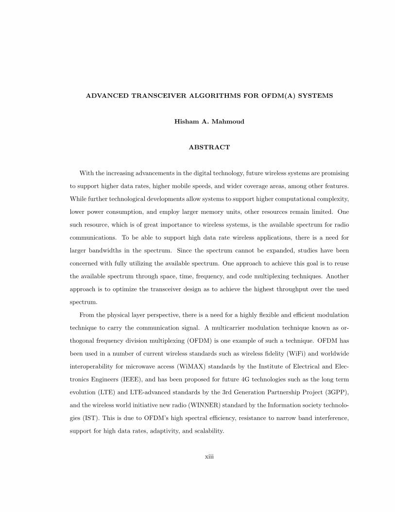
With the increasing advancements in the digital technology, future wireless systems are promising
to support higher data rates, higher mobile speeds, and wider coverage areas, among other features.
While further technological developments allow systems to support higher computational complexity,
lower power consumption, and employ larger memory units, other resources remain limited. One
such resource, which is of great importance to wireless systems, is the available spectrum for radio
communications. To be able to support high data rate wireless applications, there is a need for
larger bandwidths in the spectrum. Since the spectrum cannot be expanded, studies have been
concerned with fully utilizing the available spectrum. One approach to achieve this goal is to reuse
the available spectrum through space, time, frequency, and code multiplexing techniques. Another
approach is to optimize the transceiver design as to achieve the highest throughput over the used
spectrum.
From the physical layer perspective, there is a need for a highly flexible and efficient modulation
technique to carry the communication signal. A multicarrier modulation technique known as or-
thogonal frequency division multiplexing (OFDM) is one example of such a technique. OFDM has
been used in a number of current wireless standards such as wireless fidelity (WiFi) and worldwide
interoperability for microwave access (WiMAX) standards by the Institute of Electrical and Elec-
tronics Engineers (IEEE), and has been proposed for future 4G technologies such as the long term
evolution (LTE) and LTE-advanced standards by the 3rd Generation Partnership Project (3GPP),
and the wireless world initiative new radio (WINNER) standard by the Information society technolo-
gies (IST). This is due to OFDM’s high spectral efficiency, resistance to narrow band interference,
support for high data rates, adaptivity, and scalability.
xiii
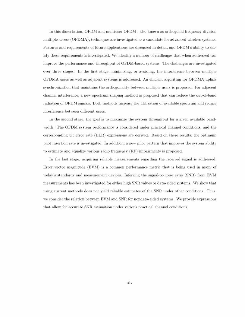
In this dissertation, OFDM and multiuser OFDM , also known as orthogonal frequency division
multiple access (OFDMA), techniques are investigated as a candidate for advanced wireless systems.
Features and requirements of future applications are discussed in detail, and OFDM’s ability to sat-
isfy these requirements is investigated. We identify a number of challenges that when addressed can
improve the performance and throughput of OFDM-based systems. The challenges are investigated
over three stages. In the first stage, minimizing, or avoiding, the interference between multiple
OFDMA users as well as adjacent systems is addressed. An efficient algorithm for OFDMA uplink
synchronization that maintains the orthogonality between multiple users is proposed. For adjacent
channel interference, a new spectrum shaping method is proposed that can reduce the out-of-band
radiation of OFDM signals. Both methods increase the utilization of available spectrum and reduce
interference between different users.
In the second stage, the goal is to maximize the system throughput for a given available band-
width. The OFDM system performance is considered under practical channel conditions, and the
corresponding bit error rate (BER) expressions are derived. Based on these results, the optimum
pilot insertion rate is investigated. In addition, a new pilot pattern that improves the system ability
to estimate and equalize various radio frequency (RF) impairments is proposed.
In the last stage, acquiring reliable measurements regarding the received signal is addressed.
Error vector magnitude (EVM) is a common performance metric that is being used in many of
today’s standards and measurement devices. Inferring the signal-to-noise ratio (SNR) from EVM
measurements has been investigated for either high SNR values or data-aided systems. We show that
using current methods does not yield reliable estimates of the SNR under other conditions. Thus,
we consider the relation between EVM and SNR for nondata-aided systems. We provide expressions
that allow for accurate SNR estimation under various practical channel conditions.
xiv
CHAPTER 1
INTRODUCTION
With the increasing demand for more applications to become wireless, wireless systems are
challenged to meet higher data rate requirements. Considering the frequency spectrum as being a
limited and valuable resource, wireless devices are faced with the necessity to utilize the available
opportunities of the spectrum and coexist with other legacy or otherwise future systems.
Studies to increase the system throughput have been concerned with improving signal detection
algorithms and reducing the impact of various practical impairments to wireless signals. Timing
and frequency offsets, radio channel propagation effects, and baseband modulator gain and phase
imbalances are examples of signal degradation sources that need to be estimated and equalized.
Minimizing the effects of these impairments increase the effective signal-to-noise ratio (SNR) at the
receiver and allow the system to support higher modulation orders and consequently higher data
rates. This approach can be considered as maximizing the system spectral efficiency for a given
allocated spectrum or bandwidth.
Recently, a new direction for utilizing the available spectrum has been suggested. This approach
calls for allowing non-licensed users, also called rental or secondary users, to operate within licensed
bands that are not heavily occupied by their intended users, also called licensed or primary users.
The secondary users, however, can only operate within licensed band given they do not interfere or
block the primary users. Recent measurements show that wide ranges of the licensed spectrum are
rarely used most of the time, while other bands are heavily occupied [1]. This indicates that the
above approach can significantly improve the spectrum utilization. This opportunistic use of the
spectrum has been proposed by the use of cognitive radio (CR) [2–4]. The formal definition of CR
has not been agreed upon at the moment, but CR can be defined as an intelligent wireless system
that is aware of its surrounding environment through sensing and measurements; a system that uses
its gained experience to plan future actions and adapt to improve the overall communication quality
1

and meet user’s needs. It is noteworthy to mention that systems based on the above approach has
also been referred to as spectrum sharing systems and overlay systems.
Considering the above two approaches to designing future wireless systems, it can be inferred that
there is a need for a physical layer (PHY) which is highly flexible, adaptable, and spectrum efficient.
On one hand, detected spectrum opportunities should be exploited by shaping the transmitted
signal accordingly. On the other hand, the system should be able to utilize available measurements
regarding the operational environment to maximize the spectral efficiency on used bands. The ability
to support multiple users is also an important aspect of wireless systems. Orthogonal frequency
division multiplexing (OFDM) technology is a special case of multicarrier systems that, we believe,
has the potential of fulfilling the aforementioned requirements.
In this chapter, a brief introduction to OFDM technology is given followed by an outline of the
remainder of this dissertation.
1.1 OFDM Technology
OFDM is one of the most widely used technologies in current communication systems. The use
of OFDM can be found in the PHY of legacy standards such as the wireless local area network
(WLAN) [5–7], wireless metropolitan area network (WMAN) standards [8, 9], and asymmetric
digital subscriber line (ADSL) [10]. In Europe, OFDM is used by the digital audio broadcasting
(DAB) [11] and terrestrial digital video broadcasting (DVB-T) [12] standards. OFDM is also a strong
candidate for future technologies such as the wireless personal area network (WPAN) standard [13]
by the Institute of Electrical and Electronics Engineers (IEEE), the long term evolution (LTE) and
LTE-Advanced [14] standards proposed by the 3rd Generation Partnership Project (3GPP), the
wireless world initiative new radio (WINNER) [15] standard proposed by the Information society
technologies (IST), and finally wireless regional area network (WRAN) standard which is known as
the first cognitive radio standard [16].
One of the main reasons for choosing OFDM as a multicarrier modulation method is due to
its robustness and high spectral efficiency specially for high data rate systems. OFDM divides the
allocated spectrum into subbands that are modulated with orthogonal subcarriers. Over frequency-
selective channels, the subcarrier bandwidth becomes smaller than the channel coherence bandwidth.
This effect allows the system to use single-tap channel equalizers, instead of the complex equalizers
that are usually needed for high bandwidth single carrier signals. Another result of this subcarrier
2

division is that every symbol is modulated over a longer time duration which reduces the inter-symbol
interference (ISI) effects caused by multipath propagation. Other advantages of OFDM include its
scalability and easy implementation using fast Fourier transform (FFT) methods.
A special case of OFDM that is of interest to this study is the multiple user OFDM technology,
known as orthogonal frequency division multiple access (OFDMA). By assigning subcarriers within
the same symbol and over different symbols to multiple users, OFDMA enables multiple user access
over frequency and time domains, respectively. In addition, by maintaining the orthogonality be-
tween subcarriers belonging to different users, OFDMA is able to achieve higher spectral efficiency
when compared to other multiple access technologies.
1.2 Dissertation Outline
For the remainder of this dissertation, advantages and challenges to OFDM technology when
applied to future communication systems are identified. Further, a number of these challenges that
improves the performance and increases the throughput of OFDM-based communication systems are
addressed. In this section, the studies presented in the remainder of this dissertation are motivated
and the following chapters are outlined.
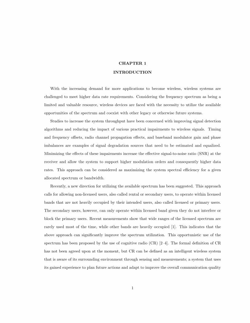
To identify challenges to OFDM-based systems, the block diagram of a generic digital commu-
nication system is considered in Fig. 1.1. The figures shows the basic elements of the PHY. At the
transmitter side, the raw bits, usually passed to the PHY by the medium access control (MAC)
layer, are encoded by introducing some redundancy to the information sequence. The encoding
process allows for forward error correction (FEC) at the receiver and improves the reliability of the
received data through error detection techniques. Encoded data are then modulated to any one
of possible waveforms to allow the signal to be transmitted over the communication channel. In
OFDM-based systems, this step also involves loading modulated symbols to orthogonal subcarri-
ers. At the receiver, demodulated symbols are compared to originally transmitted symbols to obtain
channel measurements such as error vector magnitude (EVM). The measurements could be obtained
either using known transmitted symbols or blindly by remodulating detected symbols.
Part of transmitted symbols are reserved for pilots or preambles. This step allows the receiver
to estimate and equalize the channel effect, mostly modeled as a filter response, imposed on the
transmitted signal. The channel effect is usually considered as the combined effects of the propaga-
tion channel and other radio frequency (RF) impairments (e.g. timing and frequency offsets, filters
3
Encoding ModulationInsert pilots/
preamble
Pulse/spectrum
shaping
DAC + RF
circuitry
Noisy
channel
ADC + RF
circuitry
Synchroniz-
ation
Channel
estimation/
equalization
DemodulationDecoding
PHY
Raw
bits
Raw
bits
Maintain
orthogonality,
reduce
interference
Optimize
performance,
increase
throughput
Obtain
measurements
Figure 1.1 Basic elements of the PHY in digital communication systems.
response). The ratio of the energy or number of symbols dedicated for pilots to the energy or number
of symbols dedicated for data is one of the factors that determine the overall system efficiency and
throughput.
The last step in the PHY is to pass the signal through a pulse shaping filter. In conventional
communication systems, this process improves the spectrum characteristics of the modulated signal
and limits or negates the ISI between consecutive symbols. In CR systems, the process may also
involve shaping the signal spectrum adaptively to fit into a desired spectrum profile which allows for
multiple rental user (RU) access or minimize interference to licensed users (LU) currently operating
within the used band.
A detailed study of OFDM advantages and challenges when used in CR systems is presented in
Chapter 2. Examining the elements discussed above, the issues to address for future wireless systems
when OFDM is employed can be divided intro three main issues:
• Maintain orthogonality and reduce interference.
• Optimize performance and increase throughput.
• Obtain signal measurements.
Fig. 1.1 shows these three issues and their relations to the PHY components.
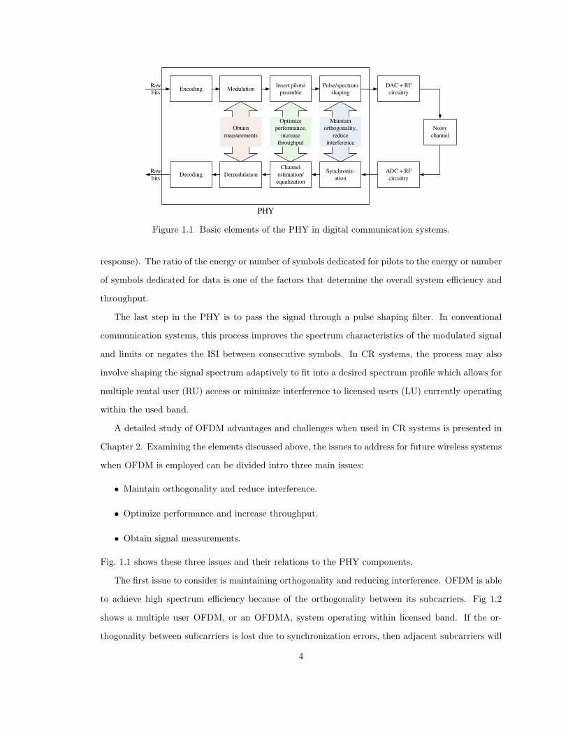
The first issue to consider is maintaining orthogonality and reducing interference. OFDM is able
to achieve high spectrum efficiency because of the orthogonality between its subcarriers. Fig 1.2
shows a multiple user OFDM, or an OFDMA, system operating within licensed band. If the or-
thogonality between subcarriers is lost due to synchronization errors, then adjacent subcarriers will
4
Frequency
Am
pli
tud
e
Licensed band
RU-1 band RU-2 band RU-3 band
Figure 1.2 OFDM subcarrier assignment within used available bands in CR systems.
interfere with each other causing inter-carrier interference (ICI). Operating under such conditions
can degrade the performance of the OFDM system significantly. This is actually one of the draw-
backs of OFDM systems; its sensitivity to timing and frequency offsets. For single user OFDM
systems, all subcarriers are modulated by the same user. In this case, the receiver only needs to
synchronize to the signal of that user to avoid synchronization errors and maintains orthogonality
between subcarriers. However, this does not apply to the uplink (UL) signal of OFDMA systems,
where different subcarriers are assigned to different users. In this case, the orthogonality is main-
tained only if all users’ signals reach the receiver synchronously. The synchronization in OFDMA
UL systems is discussed in detail in Chapter 3.
Considering CR systems, there are possibly one or more LU operating within the used band.
In this case, the OFDM system needs to avoid interfering with these LU bands through spectrum
shaping techniques. Although disabling the set of subcarriers that lay within the licensed band as
shown in Fig. 1.2 can reduce the radiation leaked to the licensed band, there is still a significant
amount of interference to the LU. The reason for this high adjacent channel interference (ACI) is due
to the high sidelobes of OFDM subcarriers. To further minimize OFDM out-of-band radiation to
neighboring bands, it is conventional to disable subcarriers that operate at the edge of used bands,
also known as guard subcarriers. This process leads to lower spectrum efficiency as the vacant bands
are not fully utilized. In Chapter 4, some of the advanced methods used to shape the spectrum of
OFDM signals are discussed. We also introduce a novel method for OFDM spectrum shaping that
can outperform current methods.
5
In the first issue discussed above, the concern is to utilize the available spectrum opportunities
while minimizing or avoiding the interference between multiple users of the same system as well
as between RUs and LUs sharing the same band. Based on the vacant bands of the spectrum
and the used spectrum shaping method, the number of usable OFDM subcarriers are determined.
Part of used subcarriers are then dedicated to pilots or preambles to aid in the channel estimation
and equalization process at the receiver. Increasing the number of pilot subcarriers improves the
channel estimation which reduces the bit error rate (BER) at the receiver. However, using too
many subcarriers for pilots reduces the overall throughput of the system. On the other hand,
an insufficient number of pilot subcarriers leads to worse channel estimation and increases the BER
which in turns decreases the system throughput. Thus, there is usually an optimum number of pilots
that maximize the system throughput depending on the channel statistics and the used channel
estimation method. The optimum pilot insertion rate for OFDM systems has been presented in
the literature. Methods that were developed for OFDM systems assumed all available pilots could
be used for channel estimation and equalization since they belong to a single user. In addition,
optimum channel estimation techniques were assumed. When considering OFDMA-UL systems, the
problem is more complicated since multiple user access means the received signal is actually a sum of
multiple signals received over different channels. Moreover, since pilots are divided among users, the
number of pilots per channel are not sufficient for optimum channel estimation techniques. Recently,
some studies investigated possible channel estimation techniques for OFDMA-UL systems. However,
these studies did not provide neither the BER performance of the system under channel estimation
errors nor the optimum pilot insertion rate. In Chapter 5, the performance of OFDMA-UL systems
over time-varying frequency-selective channels is considered. We provide BER expressions for the
received signal under channel estimation errors. Based on the derived expressions, an optimum
pilot insertion rate, in both time and frequency directions, that maximizes the system throughput
is identified.
A direct conversion receiver, also known as zero-IF receiver, is an attractive architecture for
OFDM systems since it avoids costly intermediate frequency (IF) filters, reduces power consumption,
and allows for easier integration than super-heterodyne structure [17]. However, direct conversion
receivers cause more distortions to the baseband signal due to the imbalance between the inphase (I)
and quadrature (Q) branches. The IQ imbalance results in a degradation in the system performance.
This drawback of direct conversion receivers becomes more significant with OFDM systems as they
6

are known to be sensitive to receiver front-end non-idealities [18]. As mentioned earlier, channel
estimation and equalization process takes into account not only the channel propagation effects but
also other impairments to the signal. In Chapter 6, the effects of IQ imbalance on OFDMA-UL
systems are considered. Methods to estimate and equalized both the multiuser channels and IQ
distortions are investigated. A novel pilot pattern is designed which is then used by two proposed
methods to efficiently mitigate signal distortions caused by the combined effects of the wireless
communication channels and IQ imbalances of multiple users. Compared to Chapter 5 where we
investigate optimum pilot insertion rate, in Chapter 6, we investigate optimum pilot patterns.
Finally, the third issue to consider is obtaining reliable measurements of the received signal
quality. BER and EVM are two primary specifications that determine the performance of the
wireless system in terms of transmitted and received symbols. While BER is useful as a conceptual
figure of merit, it suffers from a number of practical drawbacks such as the complexity and delay
required for calculation. In addition, it has limited diagnostic value. If the BER value measured
exceeds accepted limits, it offers no clue regarding the probable cause or source of signal degradation.
Hence, EVM has been considered as a viable alternative test method when looking for a figure of
merit in wireless channels. EVM is calculated by comparing originally modulated symbols (at the
output of the modulator) to received symbols (at the input to the demodulator) in data aided
cases. In nondata aided cases, detected symbols at the output of the demodulator are remodulated
and used as a reference instead. EVM can offer insightful information on the various transmitter
imperfections, including carrier leakage, IQ mismatch, nonlinearity, local oscillator (LO) phase noise
and frequency error [19]. Requirements on EVM are already part of most wireless communications
standards such as the IEEE 802.11a-1999 standard [6] and the IEEE 802.16e-2005 standard [9].
Relating EVM to other performance metrics such as SNR and BER is an important research topic
as these relations allow the reuse of already available EVM measurements to infer more information
regarding the communication system. Moreover, using EVM measurements could reduce the system
complexity by getting rid of the need to have separate modules to estimate or measure other metrics.
In Chapter 7, we consider the relation between EVM and SNR for nondata-aided receivers. The
signal degradation sources are modeled as additive white Gaussian noise (AWGN), Rayleigh fading
channels, and IQ imbalances. The exact value of EVM for nondata-aided symbol detection is derived
and expressed in terms of the SNR. The results show that SNR can be accurately estimated using
measured EVM even when symbol sequences are unknown, and the SNR level is low.
7
In the remainder of this chapter, a more detailed outline of the following chapters in this disser-
tation are introduced.
1.2.1 Chapter 2: OFDM for Cognitive Radio, Merits and Challenges
CR is a novel concept that allows wireless systems to sense the environment, adapt, and learn
from previous experience to improve the communication quality. However, CR needs a flexible and
adaptive PHY in order to perform the required tasks efficiently. In this chapter, CR systems and
their requirements of the PHY are discussed and OFDM technique is investigated as a candidate
transmission technology for CR. The challenges that arise from employing OFDM in CR systems
are identified. The cognitive properties of some OFDM-based wireless standards are also discussed
in order to indicate the technical trend toward a more CR.1
1.2.2 Chapter 3: Synchronization in OFDMA Uplink Systems
Synchronization is one of the most important processes in the OFDMA-based systems such as
the mobile worldwide interoperability for microwave access (WiMAX) standard. Synchronization
between a base station (BS) and all users within a cell are done through what is known as the ranging
process. In this chapter, the details of the ranging process are presented. Some of the proposed
algorithms, as well as a novel algorithm to carry out a successful ranging process are discussed.
Performance curves and computational complexity comparisons between proposed algorithm and
current algorithms are presented. The system performance is evaluated for both AWGN channels
and practical frequency-selective fading channels with multiuser interference (MUI). It is shown
that the proposed algorithm offers a reduced complexity ranging method that can be employed in
practical OFDMA-based BSs.2
1.2.3 Chapter 4: Spectrum Shaping of OFDM-based Cognitive Radio Signals
In this chapter, OFDM spectrum shaping using various techniques to reduce ACI is investi-
gated. The trade-offs between interference level and spectral efficiency, power consumption, and
computational complexity are discussed. Simulation results along with detailed analysis showing
the advantages and disadvantages of considered technique are presented. In addition, we introduce
a new method for OFDM sidelobe suppression. An extension is added to OFDM symbols that is
1Contents of this chapter were published in parts in [20, 21].2Contents of this chapter were published in parts in [22, 23].
8

calculated using optimization methods to minimize ACI while keeping the extension power at an
acceptable level. Using this technique, interference to adjacent signals is reduced significantly at
the cost of a small decrease in the useful symbol energy. The proposed method can be used by CR
systems to shape the spectrum of OFDM signals and to minimize interference to LUs, or to reduce
the size of guard bands used in conventional OFDM systems.3
1.2.4 Chapter 5: Analysis and Optimization of OFDMA Uplink Systems Over Time-Varying Frequency-Selective Rayleigh Fading Channels
Channel estimation and equalization is one the processes that significantly impacts the over-
all performance of OFDMA systems. In this chapter, the performance of OFDMA-UL systems
over time-varying frequency-selective Rayleigh fading channels is investigated. Expressions for the
BER performance for quadrature phase shift keying (QPSK) and quadrature amplitude modulation
(QAM) signals under channel estimation errors are derived. Based on BER performance, the opti-
mum pilot insertion rates for a tile-based OFDMA system to maximize the overall system throughput
are investigated.
1.2.5 Chapter 6: IQ Imbalance Correction for OFDMA Uplink Systems
Direct conversion receivers are attractive for low cost systems as they avoid IF filters. However,
the direct conversion from RF to complex I and Q baseband signals in one mixing step introduces
additional front-end distortions. These IQ distortions lead to a degradation in the system perfor-
mance. The problem becomes more significant in OFDMA systems where multiple user signals with
different IQ impairments are combined in the UL signal. In this chapter, detection methods for
OFDMA-UL signals corrupted by IQ distortions are investigated. The received signal as a function
of transmitted signals, IQ parameters, and communication channels is mathematically formulated.
We designed a novel pilot pattern that is used by two proposed estimation and compensation meth-
ods for the IQ impairments in the signal. Through simulations, proposed methods were shown to
significantly improve the system performance.4
3Contents of this chapter were published in parts in [24, 25].4Contents of this chapter were published in parts in [26].
9
1.2.6 Chapter 7: Error Vector Magnitude Based SNR Estimation in Blind Receivers
EVM is one of the widely accepted figure of merits used to evaluate the quality of communication
systems. In the literature, EVM has been related to SNR for data-aided receivers, where preamble
sequences or pilots are used to measure the EVM, or under the assumption of high SNR values. In
this chapter, this relation is examined for nondata-aided receivers and is shown to perform poorly,
especially for low SNR values or high modulation orders. The EVM for nondata-aided receivers is
then evaluated and its value is related to the SNR for QAM and pulse amplitude modulation (PAM)
signals over AWGN channels and Rayleigh fading channels, and for systems with IQ imbalances.
The results show that derived equations can be used to reliably estimate SNR values using EVM
measurements that are made based on detected data symbols. Thus, presented work can be quite
useful for measurement devices such as vector signal analyzers (VSA) or other wireless standards,
where EVM measurements are readily available.5
5Contents of this chapter were published in parts in [27].
10

CHAPTER 2
OFDM FOR COGNITIVE RADIO: MERITS AND CHALLENGES
2.1 Introduction
With emerging technologies and with the increasing number of wireless devices, the radio spec-
trum is becoming increasingly congested everyday. On the other hand, measurements show that
wide ranges of the spectrum are rarely used most of the time, while other bands are heavily used.
Depending on the location, time of the day, and frequency bands, the spectrum is actually found
to be underutilized. However, those unused portions of the spectrum are licensed and thus cannot
be used by systems other than the license owners. Hence, there is a need for a novel technology
that can benefit from these opportunities. cognitive radio (CR) arises to be a tempting solution to
spectral crowding problem by introducing the opportunistic usage of frequency bands that are not
heavily occupied by licensed users (LU) [2, 4]. CR can be defined as an intelligent wireless system
that is aware of its surrounding environment through sensing and measurements; a system that uses
its gained experience to plan future actions and adapt to improve the overall communication quality
and meet user’s needs.
A main aspect of CR is to autonomously exploit locally unused spectrum to improve spectrum
utilization. Other aspects include interoperability across several networks, devices, and protocols;
roaming across borders while being able to stay in compliance with local regulations; adapting the
system, transmission, and reception parameters without user intervention; and having the ability to
understand and follow actions and choices taken by their users to learn and become more responsive
over time. The focus of this chapter is the first aspect, i.e. CR’s ability to sense and be aware of its
operational environment, and dynamically adjust its radio operating parameters accordingly. For
CR to achieve this objective, the physical layer (PHY) needs to be highly flexible and adaptable.
A special case of multicarrier transmission known as orthogonal frequency division multiplexing
(OFDM) is one of the most widely used technologies in current wireless communications systems.
11
OFDM has the potential of fulfilling the aforementioned requirements of CR inherently or with minor
modifications. Because of its attractive features, OFDM has been successfully used in numerous
wireless standards and technologies. We believe that OFDM will play an important role in realizing
CR concept as well by providing a proven, scalable, and adaptive technology for air interface.
In this chapter, OFDM technique is investigated as a candidate for CR systems. CR features and
requirements are discussed in detail, and OFDM’s ability to satisfy these requirements is explained.
In addition, we go through the challenges that arise from employing OFDM technology in CR.
This chapter is organized as follows. The basic system model of OFDM systems is introduced in
Section 2.2. In Section 2.3, the structure of an OFDM-based CR is presented. Section 2.4 discusses
the merits of OFDM technology and its advantages when employed by CR systems. Challenges to a
practical OFDM-based CR system and possible solutions are addressed in Section 2.5. Section 2.6
looks into present and future technologies that use OFDM with Cognitive features. Section 2.7
concludes the chapter.
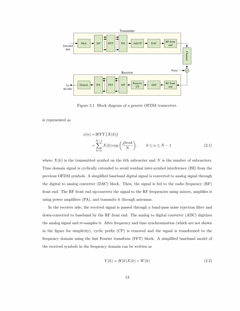
2.2 A Basic OFDM System Model
A simplified block diagram of a basic OFDM system is given in Fig. 2.1. In a multipath fading
channel, due to the frequency selectivity, each subcarrier can have different attenuation. The power
on some subcarriers may be significantly less than the average power because of deep fades. As a
result, the overall bit error rate (BER) may be largely dominated by a few subcarriers with the lowest
power level. To reduce the degradation of system performance due to this problem, channel coding
can be used prior to the modulation of the bits. Channel coding can reduce the BER significantly
depending on the code rate, decoder complexity, signal-to-noise ratio (SNR) level among other
factors. Interleaving is also applied to randomize the occurrence of bit errors and introduce system
immunity to burst errors. Coded and interleaved data bits are then mapped to the constellation
points to obtain data symbols. This step is represented by the modulation block of Fig. 2.1. The
serial data symbols are then converted to parallel data symbols which are fed to the inverse fast
Fourier transform (IFFT) block to obtain the time domain OFDM symbols. Time domain samples
12
Mod. S/P IFFT P/S Add CP DACRF front
end
+
Demod. P/S FFT S/PRemove
CPADC
RF front
end
Ch
ann
el
Noise
Encoded
data
To
decoder
Transmitter
Receiver
Figure 2.1 Block diagram of a generic OFDM transceiver.
is represented as
x(n) = IFFT {X(k)}
=
N−1∑
k=0
X(k) exp
(2πnk
N
), 0 ≤ n ≤ N − 1 (2.1)
where X(k) is the transmitted symbol on the kth subcarrier and N is the number of subcarriers.
Time domain signal is cyclically extended to avoid residual inter-symbol interference (ISI) from the
previous OFDM symbols. A simplified baseband digital signal is converted to analog signal through
the digital to analog converter (DAC) block. Then, the signal is fed to the radio frequency (RF)
front end. The RF front end up-converts the signal to the RF frequencies using mixers, amplifies it
using power amplifiers (PA), and transmits it through antennas.
In the receiver side, the received signal is passed through a band-pass noise rejection filter and
down-converted to baseband by the RF front end. The analog to digital converter (ADC) digitizes
the analog signal and re-samples it. After frequency and time synchronization (which are not shown
in the figure for simplicity), cyclic prefix (CP) is removed and the signal is transformed to the
frequency domain using the fast Fourier transform (FFT) block. A simplified baseband model of
the received symbols in the frequency domain can be written as
Y (k) = H(k)X(k) + W (k) (2.2)
13
Frequency
Am
pli
tude
Subcarrier
spacing
Total Bandwidth
Figure 2.2 OFDM waveform.
where Y (k) is the received symbol on the kth subcarrier, H(k) is the frequency response of the
channel on the same subcarrier, and W (k) is the additive noise plus interference sample which is
usually assumed to be a Gaussian variable with zero mean and variance of N0/2. Note that OFDM
converts the convolution in time domain into multiplication in frequency domain, and hence simple
one-tap frequency domain equalizers can be used to recover the transmitted symbols. After FFT,
the symbols are demodulated, deinterleaved and decoded to obtain the transmitted information bits.
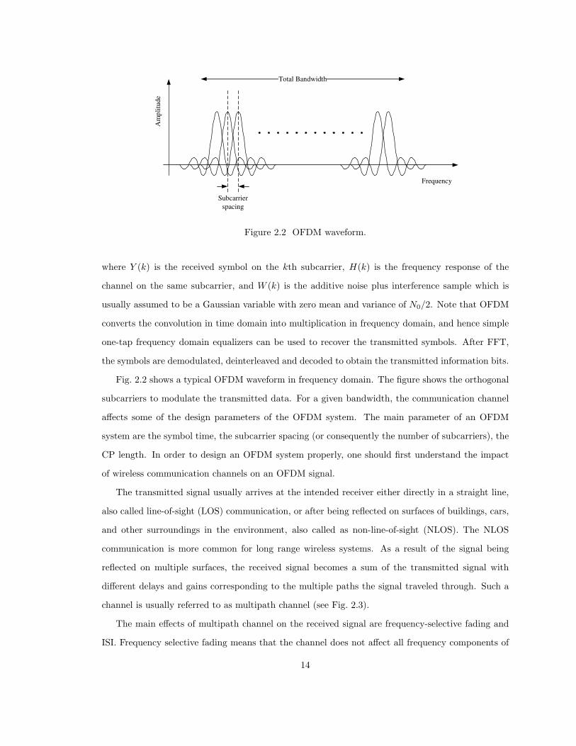
Fig. 2.2 shows a typical OFDM waveform in frequency domain. The figure shows the orthogonal
subcarriers to modulate the transmitted data. For a given bandwidth, the communication channel
affects some of the design parameters of the OFDM system. The main parameter of an OFDM
system are the symbol time, the subcarrier spacing (or consequently the number of subcarriers), the
CP length. In order to design an OFDM system properly, one should first understand the impact
of wireless communication channels on an OFDM signal.
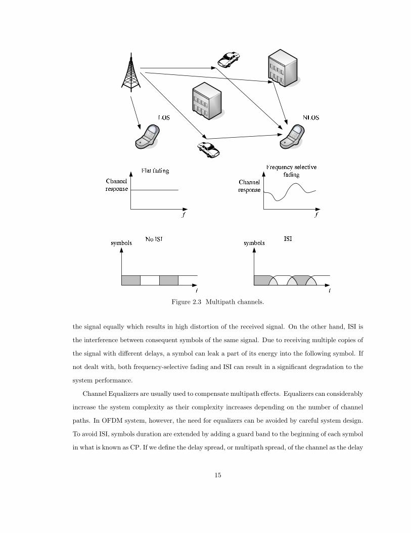
The transmitted signal usually arrives at the intended receiver either directly in a straight line,
also called line-of-sight (LOS) communication, or after being reflected on surfaces of buildings, cars,
and other surroundings in the environment, also called as non-line-of-sight (NLOS). The NLOS
communication is more common for long range wireless systems. As a result of the signal being
reflected on multiple surfaces, the received signal becomes a sum of the transmitted signal with
different delays and gains corresponding to the multiple paths the signal traveled through. Such a
channel is usually referred to as multipath channel (see Fig. 2.3).
The main effects of multipath channel on the received signal are frequency-selective fading and
ISI. Frequency selective fading means that the channel does not affect all frequency components of
14
� ���������������� ���
�������
�������
������������� ��������� ������������������� ������� �� � �
Figure 2.3 Multipath channels.
the signal equally which results in high distortion of the received signal. On the other hand, ISI is
the interference between consequent symbols of the same signal. Due to receiving multiple copies of
the signal with different delays, a symbol can leak a part of its energy into the following symbol. If
not dealt with, both frequency-selective fading and ISI can result in a significant degradation to the
system performance.
Channel Equalizers are usually used to compensate multipath effects. Equalizers can considerably
increase the system complexity as their complexity increases depending on the number of channel
paths. In OFDM system, however, the need for equalizers can be avoided by careful system design.
To avoid ISI, symbols duration are extended by adding a guard band to the beginning of each symbol
in what is known as CP. If we define the delay spread, or multipath spread, of the channel as the delay
15

between the first and last received paths over the channel, the CP should be equal to or longer than
that delay. On the other hand, the frequency-selective fading is avoided by decreasing the subcarrier
spacing or consequently increasing the number of subcarriers. We define the channel coherence
bandwidth as the bandwidth over which the channel could be considered flat. Since ODFM signal
can be considered as group of narrow band signals, by increasing the number of subcarriers, the
bandwidth of each subcarrier, also known as the subcarrier spacing, becomes narrower. By choosing
the subcarrier spacing to be less than the coherence bandwidth of the channel, each subcarrier is
going to be affected by a flat channel and thus complex channel equalization is not needed.
Another channel effect that should be considered in the OFDM systems design is the mobility.
For fixed communication systems, the channel can be considered constant over time. However, if
either of the transmitter or the receiver is mobile, the channel is going to vary over time resulting in
fast fading of the received signal. Coherence time of the channel is defined as the time over which the
channel is considered constant. To avoid fast fading effect, OFDM symbol time is chosen to be equal
to or shorter than the coherence time of the channel. In the frequency domain, mobility results in a
frequency spread of the signal which is dependent on the operating frequency and the relative speed
between the transmitter and receiver, also know as Doppler spread [28]. Doppler spread of OFDM
signals results in inter-carrier interference (ICI) which can be reduced by increasing the subcarrier
spacing.
In conclusion, while increasing the symbol time reduces ISI effect, shorter symbol time is desirable
to avoid fast fading of the signal. And while decreasing subcarrier spacing reduces ICI, narrower
subcarrier spacing helps avoiding frequency selectivity. As a matter of fact, there exist an optimum
value of these parameters that should be used to improve the system performance [29].
In the aforementioned, a single user system model is represented, where the available channel is
used by a single user. Note that OFDM by itself is not a multiple access technique. However, it can be
combined with existing multiple accessing methods to allow multiple users to access to the available
channel. Some of the most common multiple access techniques that can be employed by OFDM
systems are time division multiple access (TDMA), carrier sense multiple accessing (CSMA) [6],
frequency division multiple accessing (FDMA), and code division multiple access (CDMA) based
schemes [30]. In addition, a mix of TDMA and FDMA known as orthogonal frequency division
multiple access (OFDMA) [31] is also possible. Note that in the above system model, the interference
from other users and other technologies, such as co-channel interference (CCI), adjacent channel
16
interference (ACI), narrow-band interference (NBI), etc.; are all folded into the noise term for the
sake of simplicity. However, in reality, when the received signal is impaired by a dominant interferer,
a more accurate model needs to be used.
2.3 OFDM-Based CR
In this chapter, we assume a CR system operating as a rental user (RU) in a licensed band. The
CR system identifies available or unused parts of the spectrum and exploit them. The goal is to
achieve maximum throughput while keeping interference to LUs to a minimum. An example of such
a CR system could be the IEEE 802.22 standard-based system where the spectrum allocated for TV
channels is reused. In this case, the TV channels are the LU and the standard-based systems are
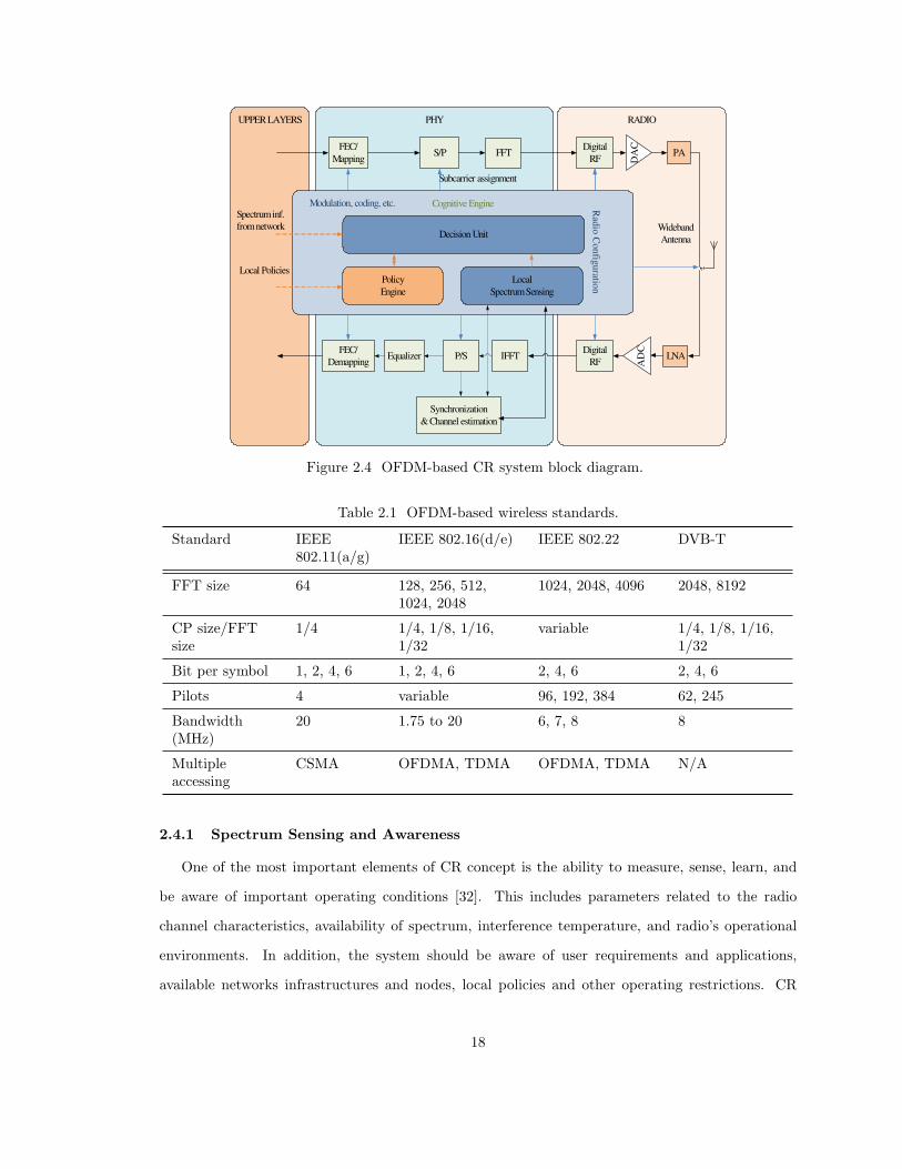
the RUs (see section 2.6.2 for more details). A block diagram of the CR-OFDM system considered
in this chapter is shown in Fig. 2.41. Note that all of the layers can interact with the Cognitive
engine. The cognitive engine is responsible for making intelligent decisions and configuring the radio
and PHY parameters. The transmission opportunities are identified by the decision unit based
on the information from policy engine as well as local and network spectrum sensing data. As
far as the PHY layer is concerned, CR can communicate with various radio access technologies
in the environment, or it can improve the communication quality depending on the environmental
characteristics, by simply changing the configuration parameters of the OFDM system (see Table 2.1
for some example parameters) and the RF interface. Note that coding type, coding rate, interleaver
pattern, and other medium access control (MAC) and higher layer functionalities, etc., should also
be changed accordingly.
2.4 Why OFDM is a Good Fit for CR
OFDM’s underlying sensing and spectrum shaping capabilities together with its flexibility and
adaptivity make it probably the best transmission technology for CR systems. In the following, we
present some of the requirements for CR and explain how OFDM can fulfill these requirements. A
summary of these requirements and strength of OFDM in meeting them are presented in Table 2.2.
1Some OFDM functions are skipped or simplified in order to keep the figure simple.
17
UPPER LAYERS RADIOPHY
Cognitive Engine
DA
CA
DC
PA
Local
Spectrum Sensing
Policy
Engine
FEC/
MappingS/P
Digital
RF
Digital
RF
FFT
IFFTP/SEqualizerFEC/
Demapping
Synchronization
& Channel estimation
r
Decision Unit
Rad
io C
on
figuratio
n
Local Policies
Spectrum inf.
from network
Modulation, coding, etc.
Wideband
Antenna
Subcarrier assignment
LNA
Figure 2.4 OFDM-based CR system block diagram.
Table 2.1 OFDM-based wireless standards.
Standard IEEE802.11(a/g)
IEEE 802.16(d/e) IEEE 802.22 DVB-T
FFT size 64 128, 256, 512,1024, 2048
1024, 2048, 4096 2048, 8192
CP size/FFTsize
1/4 1/4, 1/8, 1/16,1/32
variable 1/4, 1/8, 1/16,1/32
Bit per symbol 1, 2, 4, 6 1, 2, 4, 6 2, 4, 6 2, 4, 6
Pilots 4 variable 96, 192, 384 62, 245
Bandwidth(MHz)
20 1.75 to 20 6, 7, 8 8
Multipleaccessing
CSMA OFDMA, TDMA OFDMA, TDMA N/A
2.4.1 Spectrum Sensing and Awareness
One of the most important elements of CR concept is the ability to measure, sense, learn, and
be aware of important operating conditions [32]. This includes parameters related to the radio
channel characteristics, availability of spectrum, interference temperature, and radio’s operational
environments. In addition, the system should be aware of user requirements and applications,
available networks infrastructures and nodes, local policies and other operating restrictions. CR
18
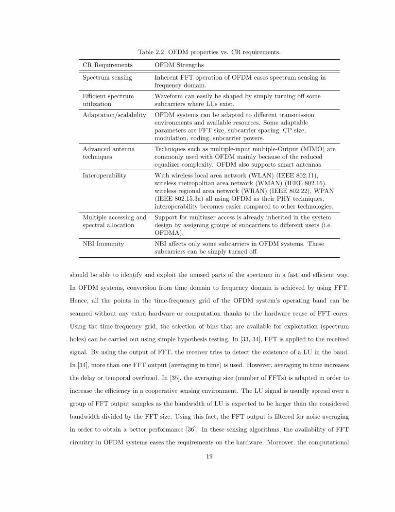
Table 2.2 OFDM properties vs. CR requirements.
CR Requirements OFDM Strengths
Spectrum sensing Inherent FFT operation of OFDM eases spectrum sensing infrequency domain.
Efficient spectrumutilization
Waveform can easily be shaped by simply turning off somesubcarriers where LUs exist.
Adaptation/scalability OFDM systems can be adapted to different transmissionenvironments and available resources. Some adaptableparameters are FFT size, subcarrier spacing, CP size,modulation, coding, subcarrier powers.
Advanced antennatechniques
Techniques such as multiple-input multiple-Output (MIMO) arecommonly used with OFDM mainly because of the reducedequalizer complexity. OFDM also supports smart antennas.
Interoperability With wireless local area network (WLAN) (IEEE 802.11),wireless metropolitan area network (WMAN) (IEEE 802.16).wireless regional area network (WRAN) (IEEE 802.22), WPAN(IEEE 802.15.3a) all using OFDM as their PHY techniques,interoperability becomes easier compared to other technologies.
Multiple accessing andspectral allocation
Support for multiuser access is already inherited in the systemdesign by assigning groups of subcarriers to different users (i.e.OFDMA).
NBI Immunity NBI affects only some subcarriers in OFDM systems. Thesesubcarriers can be simply turned off.
should be able to identify and exploit the unused parts of the spectrum in a fast and efficient way.
In OFDM systems, conversion from time domain to frequency domain is achieved by using FFT.
Hence, all the points in the time-frequency grid of the OFDM system’s operating band can be
scanned without any extra hardware or computation thanks to the hardware reuse of FFT cores.
Using the time-frequency grid, the selection of bins that are available for exploitation (spectrum
holes) can be carried out using simple hypothesis testing. In [33, 34], FFT is applied to the received
signal. By using the output of FFT, the receiver tries to detect the existence of a LU in the band.
In [34], more than one FFT output (averaging in time) is used. However, averaging in time increases
the delay or temporal overhead. In [35], the averaging size (number of FFTs) is adapted in order to
increase the efficiency in a cooperative sensing environment. The LU signal is usually spread over a
group of FFT output samples as the bandwidth of LU is expected to be larger than the considered
bandwidth divided by the FFT size. Using this fact, the FFT output is filtered for noise averaging
in order to obtain a better performance [36]. In these sensing algorithms, the availability of FFT
circuitry in OFDM systems eases the requirements on the hardware. Moreover, the computational
19

0 5 10 15 20 25
Subcarrier index
Am
pli
tud
e
0 5 10 15 20 25
Subcarrier indexA
mp
litu
de
Sensing...
Shaping...
Licensed users
Figure 2.5 Spectrum sensing and shaping using OFDM.
requirements of the spectrum sensing algorithm is reduced as the receiver already applies FFT to the
received signal in order to transform the received signal into frequency domain for data detection.
2.4.2 Spectrum Shaping
After a CR system scans the spectrum and identifies active LUs, other RUs, and available
opportunities; comes the next step: spectrum shaping. Ideally, it is desired to allow RUs to freely
use available bands in the spectrum. It is desired to have a flexible spectrum mask and have control
over waveform parameters such as signal bandwidth, power level, and center frequency. OFDM
systems can provide such flexibility thanks to the unique nature of OFDM signaling. By disabling a
set of subcarriers, the spectrum of OFDM signals can be adaptively shaped to fit into the required
spectrum mask2. Assuming the spectrum mask is already known to the CR system, choosing the
disabled subcarriers is a relatively simple process.
An example of spectrum sensing and shaping procedures in OFDM-based CR systems is illus-
trated in Fig. 2.5. The two LUs are detected using the output of the FFT block, and subcarriers
that can cause interference to these LUs are turned off. The transmitter then uses the unoccupied
part of the spectrum for signal transmission.
2See Section 2.5.5 for more details and for more advanced algorithms.
20
2.4.3 Adapting to the Environment
Adaptivity is one of the key requirements of CR. By combining gathered information (awareness)
with knowledge of current system capabilities and limitations, CR can perform various tasks. CR
can adapt its waveform to interoperate with other friendly communication devices, choose the most
appropriate communication channel or network for transmission, and allocate best frequency to
transmit in a free band of the spectrum. The system waveform can also be adapted to compensate
for channel fading, and nullify any interfering signal. OFDM offers a great flexibility in this regard as
the number of parameters for adaptation is quite large [37]. An OFDM-based system can adaptively
change the modulation order, coding, and transmit power of each individual subcarrier based on user
needs or the channel quality [38]. This adaptive allocation can be optimized to achieve various goals
such as increasing the system throughput, reducing BER, limiting interference to LUs, increasing
coverage, or to prolong unit battery life. In multiuser OFDM systems, subcarriers allocation to users
can be done adaptively as well to achieve the same goals [39].
One of the attractive features of OFDM for broadband communications is its ability to operate
using simple one tap equalizers, in the frequency domain. To maintain this feature, the subcarrier
spacing in set to be less than the channel coherence bandwidth. In addition, to avoid ISI, the
system appends a CP to each symbol with a duration longer than the channel maximum delay
spread. Based on estimated channel parameters, an OFDM-based CR system can adaptively change
the length of the CP to maintain an ISI-free signal while maximizing the system throughput [29].
Similarly, OFDM system can adaptively change the subcarrier spacing to reduce ICI or peak-to-
average-power ratio (PAPR) [29], the data subcarrier interleaving to reduce BER [40], or even the
used pilot patterns [41].
The adaptivity in OFDM systems can be performed either at algorithm level or at parameter
level. In classical wireless systems, usually algorithm parameters, e.g. coding rate, have been adapted
in order to optimize the transmission. However, in cognitive OFDM systems, algorithm type, e.g.
channel coding type, can also be adapted in order to achieve interoperability with other systems
and/or to further optimize system performance. To achieve such adaptivity, a fully configurable
hardware platform would be needed.
21

2.4.4 Advanced Antenna Techniques
Advanced antenna techniques are not necessarily required for CRs. However, they are desirable
as they provide better spectral efficiency which is the primary motivation for CR. Smart antennas
and multiple-input multiple-Output (MIMO) systems can be used to exploit the spatial dimension
of spectrum space, e.g. through beam forming, to improve the efficiency. In essence, multi-antenna
systems can help to find spectral opportunities in the spatial domain and can help to exploit these
opportunities in full. The use of MIMO techniques offers several important advantages including
spatial degree of freedom, increased spectral efficiency and diversity [42]. These advantages can be
used to increase the spectrum utilization of the overall system. Furthermore, beamforming, diversity
combining, and space-time equalization can also be applied to cognitive OFDM systems. Another
application of adaptive antenna techniques is the reduction of the interference in OFDM systems [43].
MIMO systems commonly employ OFDM as their transmission technique because of simple
diversity combination and equalization, particularly at high data rates. In MIMO-OFDM, the
channel response becomes a matrix. Since each tone can be equalized independently, the complexity
of space-time equalizers is avoided and signals can be processed using relatively straightforward
matrix algebra. Moreover, the advantages of OFDM in multipath are preserved in MIMO-OFDM
system as frequency selectivity caused by multipath increases the capacity.
2.4.5 Multiple Accessing and Spectral Allocation
The resources available to a CR have to be shared among users. Several techniques can be
used to achieve such a task. OFDM supports well-known multiple accessing techniques such as
TDMA, FDMA and CSMA. Moreover, CDMA can be used together with OFDM, in which case the
transmission is known as multi-carrier code division multiple access (MC-CDMA) or multicarrier
direct spread code division multiple access (DS-CDMA).
OFDMA, a special case of OFDM, has gained significant attention recently with its usage in fixed
and mobile worldwide interoperability for microwave access (WiMAX) standard [9]. In OFDMA,
subcarriers are grouped into sets each of which is assigned to a different user. Interleaved, random-
ized, or clustered subcarrier assignment schemes can be used. Therefore, OFDMA offers very flexible
multiple accessing and spectral allocation capability for CR without any extra hardware complexity.
The allocation of subcarriers can be tailored according to the spectrum availability. The flexibility
22
WAN
IEEE 802.22
3GPP*
MAN
IEEE 802.16
WiMAX
HIPERMAN
LAN
IEEE 802.11a/g
Wi-Fi
HIPERLAN
PAN
IEEE 802.15.3a
(MB-OFDM)*
* Proposed
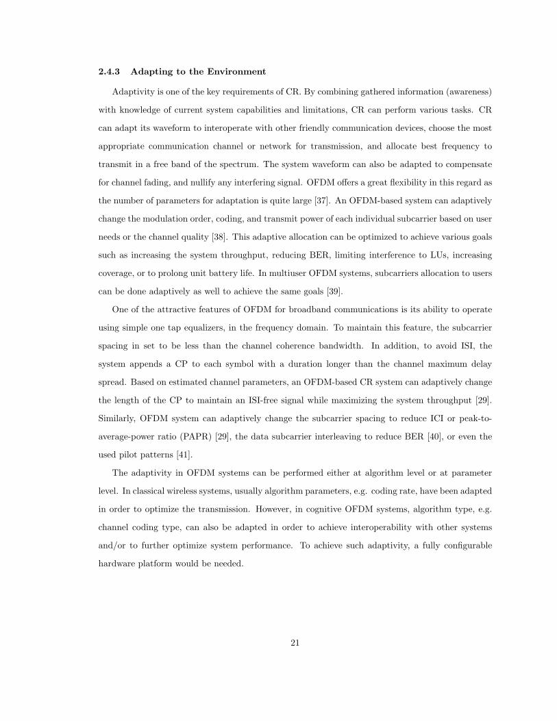
Figure 2.6 OFDM-based wireless technologies.
and support of OFDM systems for various multiple accessing techniques enable interoperability and
accelerate the adaptation of CR in future wireless systems.
2.4.6 Interoperability
Interoperability is defined as the ability of two or more systems or components to exchange
information and to use the information that has been exchanged [44]. Since CR systems may have
to deal with LUs as well as other RUs, the ability to detect and encode the existing signals within
the used band can improve the performance of CR systems. Furthermore, some recent unfortunate
disasters manifested the importance of interoperability in terms of wireless communications for the
first responders. CR has the potential to improve the disaster relief operations by developing the
coordination among first responders [45].
To achieve interoperability, OFDM is one of the best signaling candidates. OFDM signaling has
been successfully used in various technologies including the IEEE 802.11a [6] and IEEE 802.11g [46]
wireless local area network (WLAN) standards, the IEEE 802.16e-2005 [9] wireless metropolitan
area network (WMAN) standard, and the European digital audio broadcasting (DAB) and digital
video broadcasting (DVB)standards. Fig. 2.6 shows some of the OFDM-based wireless technologies
according to communication range. As shown in this figure, OFDM has been used in both short range
and long range communication systems. Hence, a CR system employing OFDM can communicate
23
OFDM
Challenges
Cognitive Radio
Challenges
Cognitive
radio-OFDM
Specific
Challenges
• ICI
• PAPR
• Synchron-
ization
• ...
• Spectrum
sensing
• Cross layer
adaptation
• Interference
avoidance
• ...
Figure 2.7 Research challenges in CR and OFDM.
with systems using other OFDM-based technologies with much ease. Only the knowledge of signal
parameters of intended users is needed (see Table 2.1). However, for such task to be successful, the
system needs to know all standard-related information required to decode the signal, such as the
data and pilot mapping to the frequency subcarriers, frame structure, and the coding type and rate.
More importantly, the RF circuitry of the CR system needs to be flexible enough to accommodate
different signal bandwidths and center frequencies. As a result, CR should be built around a software
defined radio (SDR) architecture to provide required flexibility to the system.
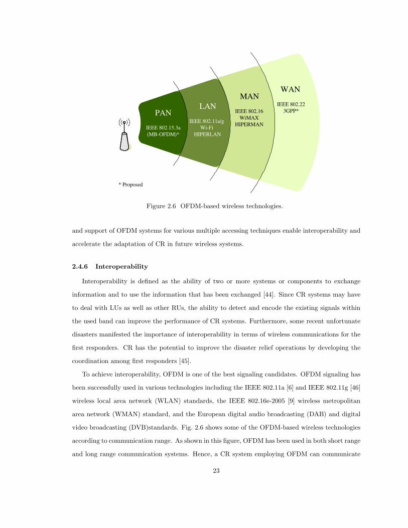
2.5 Challenges to Cognitive OFDM Systems
As an intelligent system with features such as awareness, adaptivity and learning, CR repre-
sents the future of wireless systems with the promise of offering solutions to various communication
problems. However, with this new technology, new challenges appear, raising interesting research
topics. Considering an OFDM-base CR system, the challenges can be grouped into three categories
as illustrated in Fig. 2.7. The first category includes the challenges that are unique to classical
OFDM systems such as PAPR, and sensitivity to frequency offset and phase noise. The second
category includes problems faced by all CRs such as spectrum sensing, cross layer adaptation, and
interference avoidance. Our main focus in this article is on the third category: challenges that arise
when OFDM technique is employed by CR systems. In the following, we discuss major challenges
24
to a practical system implementation as well as some of the proposed approaches for solving these
challenges.
2.5.1 Multiband OFDM System Design
So far we have considered the more conventional single-band OFDM (SB-OFDM) systems. In
SB-OFDM systems, the available portion of the spectrum is occupied by a single OFDM signal. If
LU exist within the used band, the CR system shapes the OFDM signal as to avoid interference
to those users as shown in Fig. 2.5. For systems utilizing wide bands of the spectrum, multi-band
signaling approach, where the total bandwidth is divided into smaller bands, can prove to be more
advantageous over using single band signaling. This appears to be more significant if the detected
free parts of the spectrum are scattered over a relatively wide band. While using a single band
simplifies the system design, processing a wide band signal requires building highly complex RF
circuitry for signal transmission/reception. High speed ADCs are required to sample and digitize
the wideband signal. In addition, higher complexity channel equalizers are also needed to capture
sufficient multipath signal energy for further processing. On the other hand, multi-band signaling
relaxes the requirements on system hardware as smaller portions of the spectrum are processed
separately. Dividing the spectrum into smaller bands allows for better spectrum allocation as well.
For OFDM-based CR, the question becomes when to use multi-band and when to use single
band. Given a certain scanned spectrum shape, choosing the number of bands depends on vari-
ous parameters. Required throughput, hardware limitations, computational complexity, number of
spectrum holes and their bandwidth, and interference level are examples of what could affect a CR
choice. We further illustrate the importance of multi-band signaling with the next example.
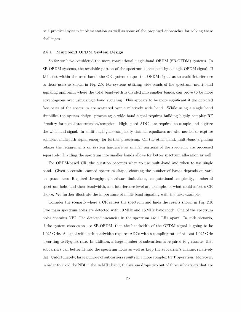
Consider the scenario where a CR senses the spectrum and finds the results shown in Fig. 2.8.
Two main spectrum holes are detected with 10 MHz and 15 MHz bandwidth. One of the spectrum
holes contains NBI. The detected vacancies in the spectrum are 1 GHz apart. In such scenario,
if the system chooses to use SB-OFDM, then the bandwidth of the OFDM signal is going to be
1.025 GHz. A signal with such bandwidth requires ADCs with a sampling rate of at least 1.025 GHz
according to Nyquist rate. In addition, a large number of subcarriers is required to guarantee that
subcarriers can better fit into the spectrum holes as well as keep the subcarrier’s channel relatively
flat. Unfortunately, large number of subcarriers results in a more complex FFT operation. Moreover,
in order to avoid the NBI in the 15 MHz band, the system drops two out of three subcarriers that are
25
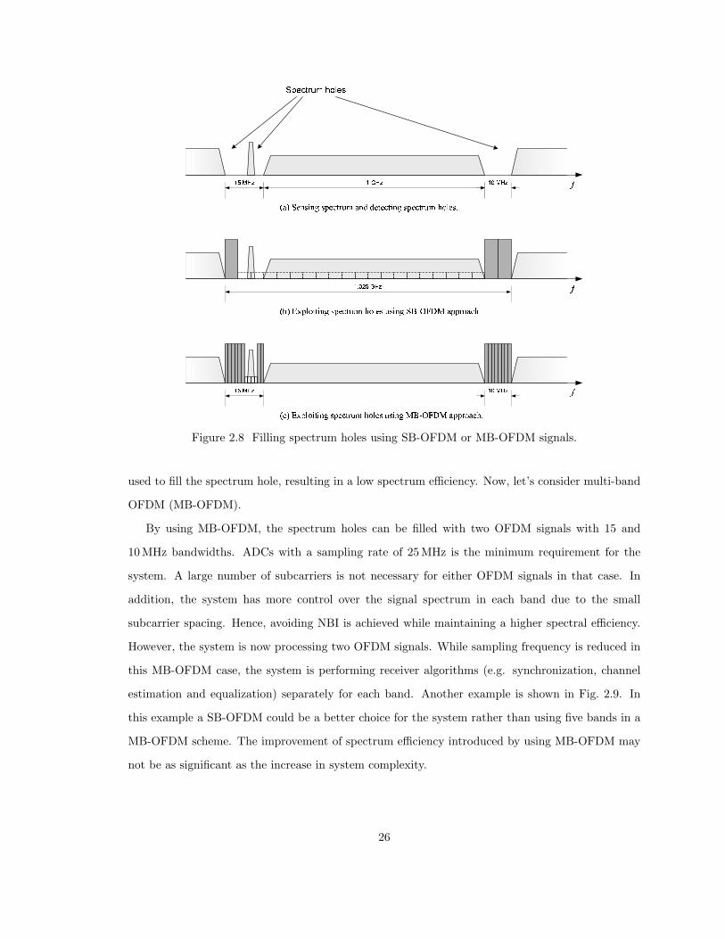
�� !" � #!" �$ !" %%
&'()*+,- ./0(1
%�2$3� #!"
�� !" �$ !"456 789:;<=<>? @9AB=CDE F;:A@ D@<>? GHIJKLM N99C;NBFO4B6 789:;<=<>? @9AB=CDE F;:A@ D@<>? MHIJKLM N99C;NBFO
4N6 GA>@<>? @9AB=CDE N>P PA=AB=<>? @9AB=CDE F;:A@O
Figure 2.8 Filling spectrum holes using SB-OFDM or MB-OFDM signals.
used to fill the spectrum hole, resulting in a low spectrum efficiency. Now, let’s consider multi-band
OFDM (MB-OFDM).
By using MB-OFDM, the spectrum holes can be filled with two OFDM signals with 15 and
10 MHz bandwidths. ADCs with a sampling rate of 25 MHz is the minimum requirement for the
system. A large number of subcarriers is not necessary for either OFDM signals in that case. In
addition, the system has more control over the signal spectrum in each band due to the small
subcarrier spacing. Hence, avoiding NBI is achieved while maintaining a higher spectral efficiency.
However, the system is now processing two OFDM signals. While sampling frequency is reduced in
this MB-OFDM case, the system is performing receiver algorithms (e.g. synchronization, channel
estimation and equalization) separately for each band. Another example is shown in Fig. 2.9. In
this example a SB-OFDM could be a better choice for the system rather than using five bands in a
MB-OFDM scheme. The improvement of spectrum efficiency introduced by using MB-OFDM may
not be as significant as the increase in system complexity.
26
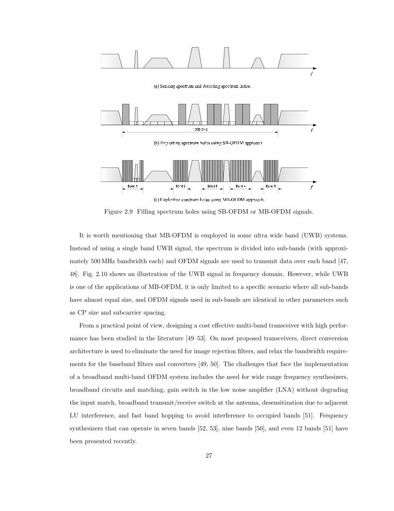
QQQ
RSTUV WXYZ[\] R Z[\] V
^_` abcdefgfhi jcklgmno pedkj njfhi qrstuvw xccmexlpy^l` abcdefgfhi jcklgmno pedkj njfhi wrstuvw xccmexlpy
^x` qkhjfhi jcklgmno xhz zkgklgfhi jcklgmno pedkjy
Z[\] {Z[\] |Z[\] UFigure 2.9 Filling spectrum holes using SB-OFDM or MB-OFDM signals.
It is worth mentioning that MB-OFDM is employed in some ultra wide band (UWB) systems.
Instead of using a single band UWB signal, the spectrum is divided into sub-bands (with approxi-
mately 500 MHz bandwidth each) and OFDM signals are used to transmit data over each band [47,
48]. Fig. 2.10 shows an illustration of the UWB signal in frequency domain. However, while UWB
is one of the applications of MB-OFDM, it is only limited to a specific scenario where all sub-bands
have almost equal size, and OFDM signals used in sub-bands are identical in other parameters such
as CP size and subcarrier spacing.
From a practical point of view, designing a cost effective multi-band transceiver with high perfor-
mance has been studied in the literature [49–53]. On most proposed transceivers, direct conversion
architecture is used to eliminate the need for image rejection filters, and relax the bandwidth require-
ments for the baseband filters and converters [49, 50]. The challenges that face the implementation
of a broadband multi-band OFDM system includes the need for wide range frequency synthesizers,
broadband circuits and matching, gain switch in the low noise amplifier (LNA) without degrading
the input match, broadband transmit/receive switch at the antenna, desensitization due to adjacent
LU interference, and fast band hopping to avoid interference to occupied bands [51]. Frequency
synthesizers that can operate in seven bands [52, 53], nine bands [50], and even 12 bands [51] have
been presented recently.
27
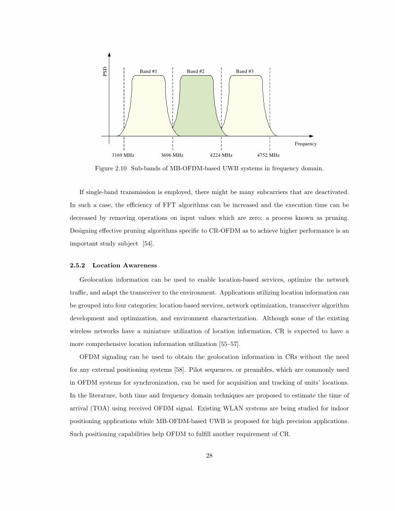
3169 MHz 3696 MHz 4224 MHz 4752 MHz
Band #1 Band #2 Band #3
Frequency
PS
D
Figure 2.10 Sub-bands of MB-OFDM-based UWB systems in frequency domain.
If single-band transmission is employed, there might be many subcarriers that are deactivated.
In such a case, the efficiency of FFT algorithms can be increased and the execution time can be
decreased by removing operations on input values which are zero; a process known as pruning.
Designing effective pruning algorithms specific to CR-OFDM as to achieve higher performance is an
important study subject [54].
2.5.2 Location Awareness
Geolocation information can be used to enable location-based services, optimize the network
traffic, and adapt the transceiver to the environment. Applications utilizing location information can
be grouped into four categories; location-based services, network optimization, transceiver algorithm
development and optimization, and environment characterization. Although some of the existing
wireless networks have a miniature utilization of location information, CR is expected to have a
more comprehensive location information utilization [55–57].
OFDM signaling can be used to obtain the geolocation information in CRs without the need
for any external positioning systems [58]. Pilot sequences, or preambles, which are commonly used
in OFDM systems for synchronization, can be used for acquisition and tracking of units’ locations.
In the literature, both time and frequency domain techniques are proposed to estimate the time of
arrival (TOA) using received OFDM signal. Existing WLAN systems are being studied for indoor
positioning applications while MB-OFDM-based UWB is proposed for high precision applications.
Such positioning capabilities help OFDM to fulfill another requirement of CR.
28

2.5.3 Signaling the Transmission Parameters
In a CR system, communication units sense the surrounding environment and gather up informa-
tion that can be used to improve the communication link. Based on gathered information, the system
selects transmission parameters such as LU bands, spectral mask, operating frequency, coding, and
modulation. While some of these parameters can be detected blindly by intended receivers, other
parameters need to be known prior to establishing a communication link. Distributing information
among communication units rather than using local sensing reduces the complexity and improves
the performance of the system. Thus, it is crucial for the success of CR to successfully distribute
such information to operational RUs.
One approach to this problem is to dedicate a communication channel for the exchange of mea-
sured information and transmission parameters among RUs. However, this requires that a channel
be predefined, or licensed, for that purpose. As a result, the ability of RUs to adaptively operate
within any given unlicensed band becomes dependent on the availability of such a channel. More-
over, as the number of operating units in the same cell increases, the amount of information that
needs to be distributed increases as well. This can result in a huge overhead that the dedicated
channel may not be able handle.
Other approaches solve the distribution problem by either reducing the information overhead
or by improving the performance of blind detectors. For example, in OFDM systems, based on
the scanned channel, waveform is adjusted by turning off some subcarriers in order to exploit the
available spectrum holes similar to what is shown in Fig. 2.5. The receivers, however, should be
informed about detected spectrum holes, or which subcarriers are deactivated. The overhead is
reduced by broadcasting the vector containing disabled subcarriers rather than exchanging the spec-
trum sensing results. One method to further reduce the overhead is proposed in [59], where the
activation/deactivation of subcarriers is performed over a block of subcarriers instead of individual
subcarriers. Hence, the signaling overhead can be reduced by a factor of the block size. On the
other hand, instead of sharing the spectrum sensing information, tone-boosting can be used to RU
of which subcarriers are disabled [60]. Once a RU detects a LU signal within the band, it sends a
tone with maximum power but with a very short time duration over the detected signal band. The
purpose is to inform other RUs that a LU is operating within this band. As a result, the probability
of interference to LUs is reduced, which is one of the main purposes of spectrum sensing. Meanwhile,
the short duration of these tones causes no significant interference to LUs.
29
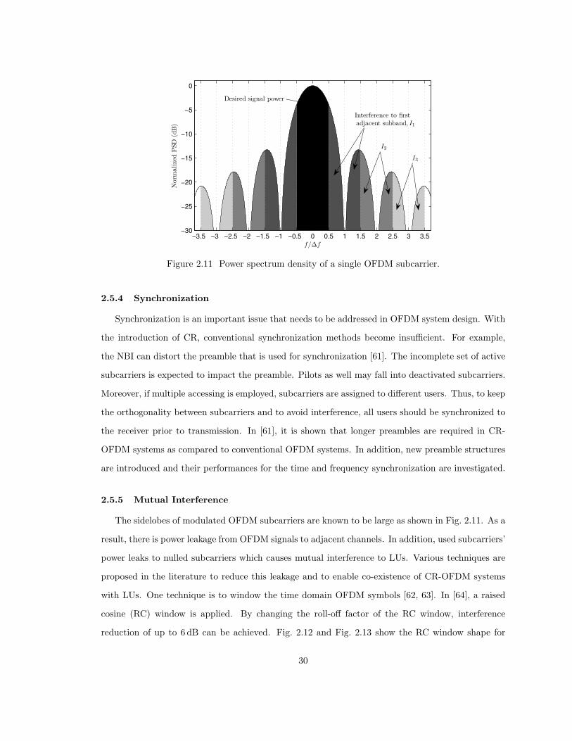
f/∆f
Norm
alize
dP
SD
(dB
)
−3.5 −3 −2.5 −2 −1.5 −1 −0.5 0 0.5 1 1.5 2 2.5 3 3.5−30
−25
−20
−15
−10
−5
0
Desired signal power
Interference to firstadjacent subband, I1
I2
I3
Figure 2.11 Power spectrum density of a single OFDM subcarrier.
2.5.4 Synchronization
Synchronization is an important issue that needs to be addressed in OFDM system design. With
the introduction of CR, conventional synchronization methods become insufficient. For example,
the NBI can distort the preamble that is used for synchronization [61]. The incomplete set of active
subcarriers is expected to impact the preamble. Pilots as well may fall into deactivated subcarriers.
Moreover, if multiple accessing is employed, subcarriers are assigned to different users. Thus, to keep
the orthogonality between subcarriers and to avoid interference, all users should be synchronized to
the receiver prior to transmission. In [61], it is shown that longer preambles are required in CR-
OFDM systems as compared to conventional OFDM systems. In addition, new preamble structures
are introduced and their performances for the time and frequency synchronization are investigated.
2.5.5 Mutual Interference
The sidelobes of modulated OFDM subcarriers are known to be large as shown in Fig. 2.11. As a
result, there is power leakage from OFDM signals to adjacent channels. In addition, used subcarriers’
power leaks to nulled subcarriers which causes mutual interference to LUs. Various techniques are
proposed in the literature to reduce this leakage and to enable co-existence of CR-OFDM systems
with LUs. One technique is to window the time domain OFDM symbols [62, 63]. In [64], a raised
cosine (RC) window is applied. By changing the roll-off factor of the RC window, interference
reduction of up to 6 dB can be achieved. Fig. 2.12 and Fig. 2.13 show the RC window shape for
30
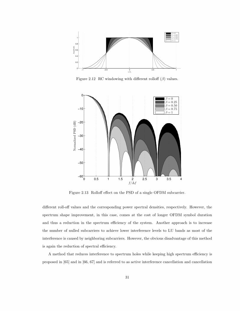
t/TsA
mplitu
de
−1 −0.5 0 0.5 10
0.2
0.4
0.6
0.8
1
β = 0β = 0.25β = 0.50β = 0.75β = 1
Figure 2.12 RC windowing with different rolloff (β) values.
f/∆f
Norm
alize
dP
SD
(dB
)
0 0.5 1 1.5 2 2.5 3 3.5 4−60
−50
−40
−30
−20
−10
0β = 0β = 0.25β = 0.50β = 0.75β = 1
Figure 2.13 Rolloff effect on the PSD of a single OFDM subcarrier.
different roll-off values and the corresponding power spectral densities, respectively. However, the
spectrum shape improvement, in this case, comes at the cost of longer OFDM symbol duration
and thus a reduction in the spectrum efficiency of the system. Another approach is to increase
the number of nulled subcarriers to achieve lower interference levels to LU bands as most of the
interference is caused by neighboring subcarriers. However, the obvious disadvantage of this method
is again the reduction of spectral efficiency.
A method that reduces interference to spectrum holes while keeping high spectrum efficiency is
proposed in [65] and in [66, 67] and is referred to as active interference cancellation and cancellation
31
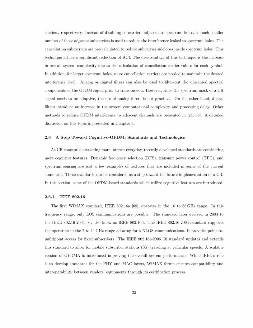
carriers, respectively. Instead of disabling subcarriers adjacent to spectrum holes, a much smaller
number of those adjacent subcarriers is used to reduce the interference leaked to spectrum holes. The
cancellation subcarriers are pre-calculated to reduce subcarrier sidelobes inside spectrum holes. This
technique achieves significant reduction of ACI. The disadvantage of this technique is the increase
in overall system complexity due to the calculation of cancellation carrier values for each symbol.
In addition, for larger spectrum holes, more cancellation carriers are needed to maintain the desired
interference level. Analog or digital filters can also be used to filter-out the unwanted spectral
components of the OFDM signal prior to transmission. However, since the spectrum mask of a CR
signal needs to be adaptive, the use of analog filters is not practical. On the other hand, digital
filters introduce an increase in the system computational complexity and processing delay. Other
methods to reduce OFDM interference to adjacent channels are presented in [24, 68]. A detailed
discussion on this topic is presented in Chapter 4.
2.6 A Step Toward Cognitive-OFDM: Standards and Technologies
As CR concept is attracting more interest everyday, recently developed standards are considering
more cognitive features. Dynamic frequency selection (DFS), transmit power control (TPC), and
spectrum sensing are just a few examples of features that are included in some of the current
standards. These standards can be considered as a step toward the future implementation of a CR.
In this section, some of the OFDM-based standards which utilize cognitive features are introduced.
2.6.1 IEEE 802.16
The first WiMAX standard, IEEE 802.16a [69], operates in the 10 to 66 GHz range. In this
frequency range, only LOS communications are possible. The standard later evolved in 2004 to
the IEEE 802.16-2004 [8]; also know as IEEE 802.16d. The IEEE 802.16-2004 standard supports
the operation in the 2 to 11 GHz range allowing for a NLOS communications. It provides point-to-
multipoint access for fixed subscribers. The IEEE 802.16e-2005 [9] standard updates and extends
this standard to allow for mobile subscriber stations (SS) traveling at vehicular speeds. A scalable
version of OFDMA is introduced improving the overall system performance. While IEEE’s role
is to develop standards for the PHY and MAC layers, WiMAX forum ensures compatibility and
interoperability between vendors’ equipments through its certification process.
32
OFDMA PHY mode is probably the most interesting mode supported by WiMAX. In this mode,
a WiMAX base station (BS) is able to support multiple fixed or mobile users at the same time. A
BS system can utilize the available channel by dividing the available subcarriers into subchannels.
A number of subchannel grouped with a number of OFDMA symbols constitutes a tile. A tile is
defined as the minimum data allocation unit [8]. The tile definition shows that the system resources
are being shared between users in two domains. The first dimension is frequency which is represented
by the number of subcarriers in each tile. The second dimension is time which is represented by
number of OFDMA symbols. Fig. 2.14 shows the OFDMA signal structure used for a WiMAX-based
system. Note that this figure is only for illustration purposes and thus the number of subcarriers or
the tile size does not necessarily reflect the actual numbers used by the standard.
A WiMAX BS can assign users different bandwidths, time durations, transmit power levels,
and modulation orders based on various parameters (see Table 2.1) such as the user carrier-to-
interference-plus-noise ratio (CINR), received signal strength indicator (RSSI) or the available band-
width. Moreover, OFDMA PHY offers multiple FFT sizes, CP sizes, and pilot allocation schemes.
The FFT size can be selected as 128, 256, 512, 1024 or 2048 depending on the transmission band-
width3. Similarly, the CP length can be set to 1/4, 1/8, 1/16 and 1/32 times the OFDM symbol
length. The CP size can be changed depending on the environment characteristics. With all these
adaptive features, WiMAX has the ability to adapt to various channel conditions and communication
scenarios.
WiMAX standard is also rich in terms of advanced antenna techniques as well. Table 2.3 shows
MIMO features available in the IEEE 802.16E-2005 standard [9]. The standard use of these tech-
niques is not directly related to CR, but rather to increase the spectral efficiency and increase the
overall throughput of the system. However, advanced antenna techniques could be used to achieve
some of the CR goals as well. For example, the CR transmitter can exploit location awareness to
focus its radiation only in the direction of intended receivers using adaptive beamforming [4, 70].
On the other hand, the CR receiver can use the same technique to adaptively cancel the interference
caused by unintended transmitters [71]. The goal in both cases would be to achieve coexistence of
WiMAX devices in unlicensed bands.
3This is known as scalable OFDMA. Various FFT sizes are used to keep the subcarrier spacing constant for differenttransmission bandwidths
33
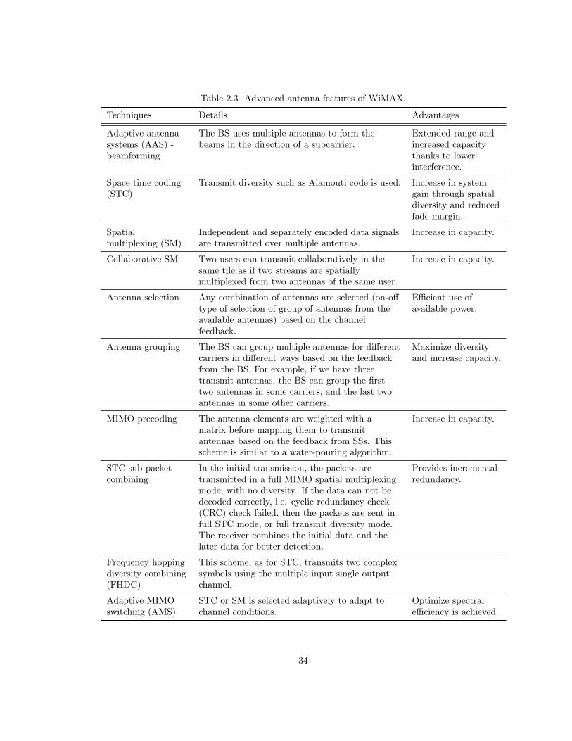
Table 2.3 Advanced antenna features of WiMAX.
Techniques Details Advantages
Adaptive antennasystems (AAS) -beamforming
The BS uses multiple antennas to form thebeams in the direction of a subcarrier.
Extended range andincreased capacitythanks to lowerinterference.
Space time coding(STC)
Transmit diversity such as Alamouti code is used. Increase in systemgain through spatialdiversity and reducedfade margin.
Spatialmultiplexing (SM)
Independent and separately encoded data signalsare transmitted over multiple antennas.
Increase in capacity.
Collaborative SM Two users can transmit collaboratively in thesame tile as if two streams are spatiallymultiplexed from two antennas of the same user.
Increase in capacity.
Antenna selection Any combination of antennas are selected (on-offtype of selection of group of antennas from theavailable antennas) based on the channelfeedback.
Efficient use ofavailable power.
Antenna grouping The BS can group multiple antennas for differentcarriers in different ways based on the feedbackfrom the BS. For example, if we have threetransmit antennas, the BS can group the firsttwo antennas in some carriers, and the last twoantennas in some other carriers.
Maximize diversityand increase capacity.
MIMO precoding The antenna elements are weighted with amatrix before mapping them to transmitantennas based on the feedback from SSs. Thisscheme is similar to a water-pouring algorithm.
Increase in capacity.
STC sub-packetcombining
In the initial transmission, the packets aretransmitted in a full MIMO spatial multiplexingmode, with no diversity. If the data can not bedecoded correctly, i.e. cyclic redundancy check(CRC) check failed, then the packets are sent infull STC mode, or full transmit diversity mode.The receiver combines the initial data and thelater data for better detection.
Provides incrementalredundancy.
Frequency hoppingdiversity combining(FHDC)
This scheme, as for STC, transmits two complexsymbols using the multiple input single outputchannel.
Adaptive MIMOswitching (AMS)
STC or SM is selected adaptively to adapt tochannel conditions.
Optimize spectralefficiency is achieved.
34
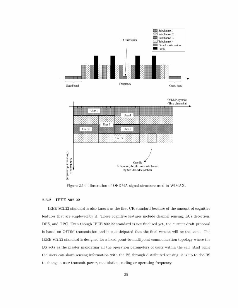
Subchannel 1
Subchannel 2
Subchannel 3
Subchannel 4
Disabled subcarriers
Pilots
FrequencyGuard band Guard band
DC subcarrier
OFDMA symbols
(Time dimension)
Su
bch
ann
els(F
requ
ency
dim
ensio
n)
One tile
In this case, the tile is one subchannel
by two OFDMA symbols
User 1
User 2
User 3
User 5
User 3
User 4
Figure 2.14 Illustration of OFDMA signal structure used in WiMAX.
2.6.2 IEEE 802.22
IEEE 802.22 standard is also known as the first CR standard because of the amount of cognitive
features that are employed by it. These cognitive features include channel sensing, LUs detection,
DFS, and TPC. Even though IEEE 802.22 standard is not finalized yet, the current draft proposal
is based on OFDM transmission and it is anticipated that the final version will be the same. The
IEEE 802.22 standard is designed for a fixed point-to-multipoint communication topology where the
BS acts as the master mandating all the operation parameters of users within the cell. And while
the users can share sensing information with the BS through distributed sensing, it is up to the BS
to change a user transmit power, modulation, coding or operating frequency.
35

One of the most distinctive features of IEEE 802.22 standard is its sensing requirements which
is based on two stages: fast sensing and fine sensing. In the fast sensing stage, a coarse algorithm
is employed, e.g. energy detector. The fine sensing stage is initiated based on the previous stage
results. However, a more detailed and powerful sensing methods are used in the second stage. The
results are returned to the BS which uses these results for managing transmissions.
One challenge in designing the IEEE 802.22 standard is the initialization of new users who desire
to communicate with the BS. Unlike current wireless technologies, frequency and time duration of
the initialization channel are not predefined. Therefore, initial users have to scan parts, if not all,
of the TV bands to find the BS operating frequency and time. In addition, users should be able to
differentiate between incumbent signals and the BS signal. This could prove to be very challenging
especially if the BS is operating over a combination of multiple frequency bands.
2.6.3 IEEE 802.11
The WLAN standard, IEEE 802.11a/g, is probably the most commonly known OFDM-based
standard. The main standard is upgraded to have cognitive features with the IEEE 802.11h and
the IEEE 802.11k standards. The IEEE 802.11h standard is designed to allow estimation of channel
characteristics and DFS. In addition, TPC is incorporated as well, providing the system with more
control over signal range and interference level. The purpose of the IEEE 802.11h standard is to
allow WLAN systems to share the 5 GHz spectrum with LUs (e.g. military radar systems).
Note that the DFS proposed for the aforementioned standards can be considered as channel
switching or frequency hopping technique. Thus, it can be applied to any transmission technology
and is not exclusive to OFDM. However, it is also noteworthy to mention that many recent published
articles have proposed new methods to facilitate DFS use for OFDM systems. OFDM subcarriers
are split into subchannels that can be disabled, enabled, or assigned to multiple users, according
to sensing measurements. These recent studies can be divided into two categories: addressing
the reduction of interference between different subchannels [24, 65–68, 72–75], and addressing the
optimization of the subcahnnel allocation process [76, 77]. In following amendments to wireless
standards, we expect that the above advanced OFDM-based techniques will be considered for DFS.
On the other hand, the IEEE 802.11k standard is proposed for radio resource management.
It defines several types of measurements such as channel load report, noise histogram report, and
station statistics report. The noise histogram report provides methods to measure interference levels
36
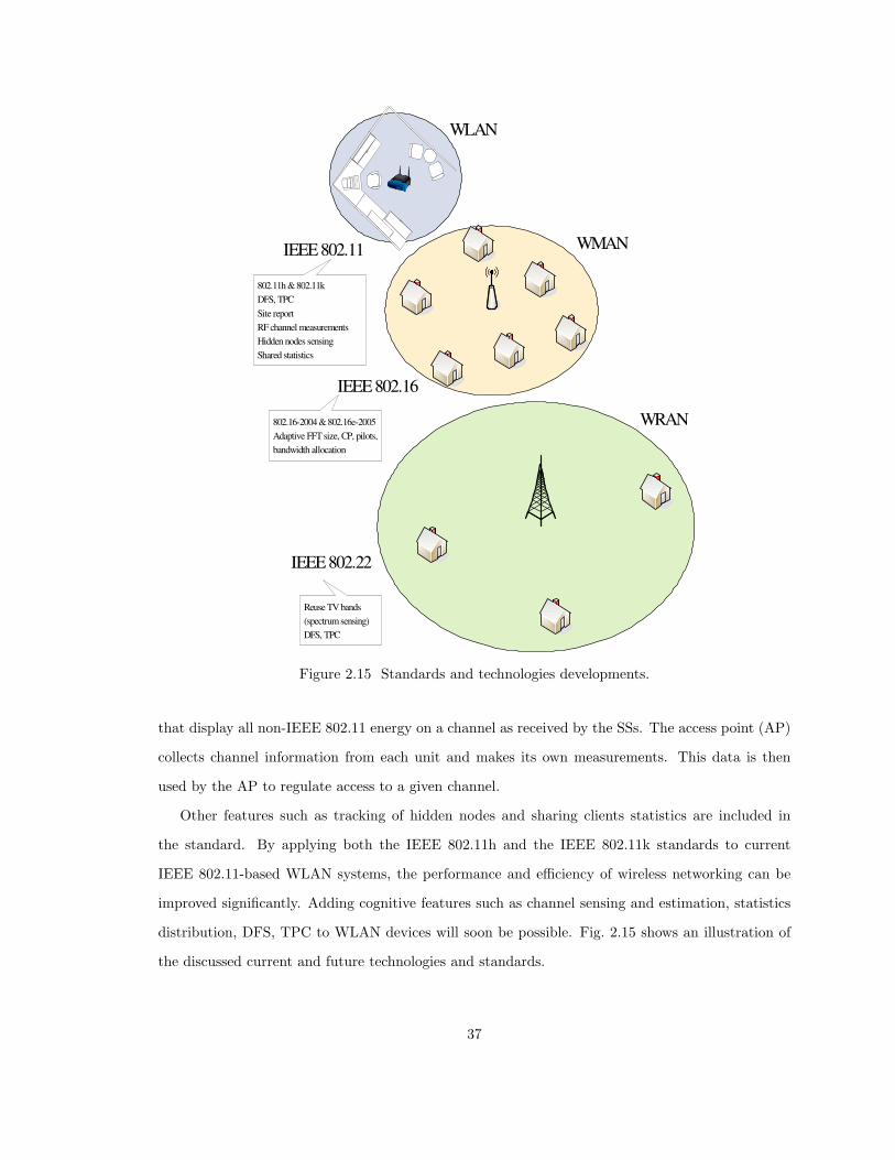
WRAN
WMAN
WLAN
IEEE 802.22
IEEE 802.16
IEEE 802.11
Reuse TV bands
(spectrum sensing)
DFS, TPC
802.16-2004 & 802.16e-2005
Adaptive FFT size, CP, pilots,
bandwidth allocation
802.11h & 802.11k
DFS, TPC
Site report
RF channel measurements
Hidden nodes sensing
Shared statistics
Figure 2.15 Standards and technologies developments.
that display all non-IEEE 802.11 energy on a channel as received by the SSs. The access point (AP)
collects channel information from each unit and makes its own measurements. This data is then
used by the AP to regulate access to a given channel.
Other features such as tracking of hidden nodes and sharing clients statistics are included in
the standard. By applying both the IEEE 802.11h and the IEEE 802.11k standards to current
IEEE 802.11-based WLAN systems, the performance and efficiency of wireless networking can be
improved significantly. Adding cognitive features such as channel sensing and estimation, statistics
distribution, DFS, TPC to WLAN devices will soon be possible. Fig. 2.15 shows an illustration of
the discussed current and future technologies and standards.
37
2.7 Conclusion
CR is an exciting and promising technology that offers a solution to the spectrum crowding
problem. On the other hand, OFDM technique is used in many wireless systems and proven as a
reliable and effective transmission method. OFDM can be used for realizing CR concept because of its
inherent capabilities that are discussed in detail in this chapter. By employing OFDM transmission in
CR systems; adaptive, aware and flexible systems capable of interoperating with current technologies
can be realized. However, the challenges identified in this chapter need to be researched further in
order to address the open issues. Practical CR systems can be developed using two approaches:
current wireless technologies can evolve to support more cognitive features over time, or new systems
that support full cognitive features can be developed. In either case, we foresee that OFDM will be
one of the dominant PHY technologies for CR.
38
CHAPTER 3
SYNCHRONIZATION IN OFDMA UPLINK SYSTEMS
3.1 Introduction
Worldwide interoperability for microwave access (WiMAX), as a relatively new technology, has
received the attention of researchers and wireless companies. This new wireless technology promises
to deliver both high data rates and long-range coverage. With the approval of the mobile WiMAX
standard (IEEE 802.16e-2005) at the beginning of the year 2006, this technology became even more
exciting. Unlike WiFi [78, 79], which is designed for indoor applications and wireless local area
network (WLAN), WiMAX is optimized for outdoor applications and wireless metropolitan area
network (WMAN).
One of the exciting aspects of WiMAX is that its medium access control (MAC) layer sup-
ports more than one physical layer (PHY) mode [9]. This feature not only enables companies to
differentiate their products from each other, but also makes WiMAX an adaptive technology that
can satisfy different needs depending on the application. One of the most promising PHY modes
supported by WiMAX standard is orthogonal frequency division multiple access (OFDMA) PHY
mode. OFDMA PHY mode enables a WiMAX base station (BS) to support multiple user access,
fixed or mobile, over both time and frequency domains. In this mode, a BS system utilizes the
channel by dividing available subcarriers into subchannels that can be assigned to multiple users in
a sophisticated and adaptive way. As a matter of fact, users can be assigned to different bandwidths,
different time durations, and different modulation orders based on various parameters such as the
user carrier-to-interference-plus-noise ratio (CINR) and the available bandwidth.
One of the problems that faces WiMAX systems, and OFDMA systems in general, is synchroniza-
tion between the BS and subscriber stations (SS) within the cell. While other orthogonal frequency
division multiplexing (OFDM) receivers can easily synchronize to the received signal [80, 81], this
is not the case for OFDMA receivers. At an OFDMA receiver, where multiple users arrive at the
39
same time, if users are not synchronized with the receiver, they will interfere with each other, and
therefore the BS will not be able to recover individual signals of each user. Hence, for OFDMA
PHY mode to work properly, all users should arrive at the BS at the same time with a considerably
high timing accuracy. This can be achieved if all users are synchronized with the BS before the
communication link is established. The standard states that for a user to join the channel, first, the
round trip delay (RTD) between the user and the BS must be known to the user [9]. This delay
estimation is used by the user to synchronize its signal such that it arrives at the BS in its allocated
time. The process in which this delay is estimated is called initial ranging, and this is mandated for
all SSs that desire to synchronize to the channel initially.
As stated in the IEEE 802.16e-2005 standard [9], the MAC layer at the BS defines a ranging
channel as a group of six (or more) subchannels, where a subchannel is a group of subcarriers that
are chosen according to a randomization formula. In addition, users are allowed to collide in this
ranging channel. Any SS that attempts to establish a communication link is required to carry out
a successful initial ranging process with the BS over the ranging channel. Once a SS senses a BS,
for network entry, it first scans for a downlink (DL) channel and synchronizes itself with the BS.
Then, the SS shall acquire transmit parameters, which are included in the uplink channel descriptor
(UCD), uplink (UL)-MAP, and DL-MAP. Using acquired parameters, the SS initiates the initial
ranging process by sending a ranging code over the UL frame. At the receiver side, the BS is
required to detect different received ranging codes and estimate the timing offset and the power for
each user that bears an initial ranging code. The BS then broadcasts the detected ranging codes
with adjustment instructions for the timing and power level. The status notifications of either a
successful ranging process or retransmission are also broadcasted.
In initial ranging, the SS chooses one of the available ranging codes randomly and transmits it
twice over two consecutive OFDMA symbols with binary phase shift keying (BPSK) modulation.
The SS should transmit the ranging code during the UL frame as long as there is a ranging oppor-
tunity. UL-MAP shows if a ranging opportunity is available through the next UL frame. Another
option is to send two consecutive ranging codes over four OFDMA symbols to increase the prob-
ability of code detection [9]. In this study, ranging over two symbols is considered since the same
concept can be applied to the four symbols case.
Synchronization for multiuser OFDM systems has been discussed in the literature. The use of
filters matched to the intended user’s subcarriers (in our case, the ranging channel subcarriers) and
40
then use of cyclic prefix (CP) redundancy to estimate the timing offset is proposed in [81]. However,
in OFDMA systems with interleaved subcarrier assignment such as WiMAX, the ranging subcarriers
are not necessarily adjacent, which makes the filtering process inapplicable. In [82], it is proposed
to synchronize users to the BS one at a time, with the assumption that other users are already
synchronized. This method cannot be used for OFDMA with multiple users colliding in the ranging
channel. In addition, this approach requires the users who are not yet synchronized to the system
to be aware of other users attempt to synchronize. Finally, in [83, 84] it is proposed to use a bank
of correlators (corresponding to number of ranging codes) in time or in frequency domain to detect
received ranging codes. The disadvantage of this approach is that the computational complexity
increases as the number of available ranging codes increases.
In this chapter, a new algorithm for OFDMA-UL synchronization or initial ranging is proposed.
System parameters are chosen based on the WiMAX standard, since it represents the most recent
standard that employs OFDMA. The proposed algorithm is examined using theoretical analysis and
computer simulations over additive white Gaussian noise (AWGN) and dispersive channels in the
presence of multiuser interference. A performance and complexity comparison between the proposed
algorithm and prior algorithms in practical system conditions are presented. It is demonstrated that
the proposed algorithm offers a significant reduction in computational complexity while carrying out
a successful initial ranging process. The reduction in complexity makes the proposed algorithm more
attractive to practical implementations of OFDMA systems. For example, the proposed algorithm
can be applied to low-cost OFDMA-based femtocell BS implementations where the number of users
per BS is limited.
The remainder of this chapter is organized as follows. The system model is introduced in Sec-
tion 3.2. Current and proposed ranging algorithms are discussed in detail in Sections 3.3 and 3.4,
respectively. In Section 3.5, the computational complexity of the proposed algorithm is calculated
and compared to current ranging algorithms. Simulation results and discussions demonstrating
the performance of the proposed ranging algorithm compared to other algorithms are presented in
Section 3.6. Finally, the conclusions are outlined in Section 3.7.
3.2 System Model
The system model is based on the IEEE 802.16e-2005 standard [9]. The UL of an OFDMA system
with N subcarriers is considered. After assigning DC and guard subcarriers, the remaining subcar-
41
riers, Nd, are grouped into Q subchannels. Each subchannel has NQ = Nd/Q subcarriers, where Q
is chosen such that Nd is an integer multiple of Q. Each user in the UL is assigned one or more sub-
channels. The BS defines a group of six subchannels (or more) for ranging. Note that the subcarriers
assigned to each subchannel are chosen randomly and thus they are not necessarily adjacent. The BS
broadcasts all the ranging information (i.e. ranging opportunities, ranging channels, ranging codes
and so on) in the UL-MAP. One ranging time slot spans two OFDMA symbol duration. The kth
ranging user signal in frequency domain is denoted as c(k)p = [c
(k)p (1), c
(k)p (2), ..., c
(k)p (L)]T , where p is
the index of the randomly chosen ranging code and L is the size of the ranging code. The signal is
then extended to N by inserting N−L zeros, which results in X(k)p = [X
(k)p (1),X
(k)p (2), ...,X
(k)p (N)]T .
Note that
X(k)p (m) =
c(k)p (n), if m = ir(n),
0, otherwise
(3.1)
where ir(n) is the index of the nth subcarrier within the ranging channel subcarriers set ir =
[ir(1), ir(2), ..., ir(L)]T . The vector X(k)p is then fed to an N -point inverse fast Fourier transform
(IFFT). The resulting signal in time domain is extended over two OFDMA symbols by repeating x(k)p
twice and adding the cyclic prefix with no phase discontinuity, where x(k)p is the time representation
of X(k)p . Note that the BS receiver uses an observation window of (N + Ng) to acquire OFDMA
symbols, where Ng is the size of the CP. Finally, the transmitted signal is denoted as s(k)p =
[s(k)p (1), s
(k)p (2), ..., s
(k)p (2N + 2Ng)]
T , where,
s(k)p =
[x(k)
p (N − Ng + 1), . . . , x(k)p (N), x(k)
p (1), . . . , x(k)p (N),
x(k)p (1), . . . , x(k)
p (N), x(k)p (1), . . . , x(k)
p (Ng)]T
. (3.2)
The transmitted signal s(k)p is then received by the BS after being corrupted by the communication
channel. In the following analysis, we assume that the channel is nondispersive and that the re-
ceived signals from multiple users are only affected by complex AWGN. However, we will evaluate
the proposed ranging algorithm performance for both AWGN and dispersive channels. A similar
approach has been used in [85] to analyze the proposed algorithm.
All users other than the users performing initial ranging are assumed to be already synchronized
to the BS. This is a valid assumption as synchronizing to the BS is mandatory before a SS can
42

establish the communication link. Hence, it is guaranteed that there is no interference from syn-
chronized user signals to the ranging channel. Note that this is not the case for ranging users as their
unsynchronized signal can cause interference to synchronized users. As this situation is unavoidable,
initial ranging SS is required by the standard to start the ranging process with minimum possible
power level. Then, as long as the SS fails to get a response from the BS, the power is increased
incrementally until a response is detected. If the maximum power level is reached and the SS still
cannot get a response from the BS, the user starts from the minimum power level and the process
is repeated. This shows how important it is for a BS to detect ranging users with the lowest signal
levels possible.
3.3 Existing Ranging Algorithms
To detect ranging codes at the BS, one approach would be to cross-correlate the received signal
with all possible ranging codes in time domain [83]. To reduce the high computational complexity
of this process, one can instead auto-correlate the received signal with its delayed replica to exploit
the repetition in the ranging code. However, for this approach to work properly, the system needs to
extract other non-ranging user signals from the received signal as the ranging users are frequency-
multiplexed with those synchronized users. Not only does such a process increase the complexity
and delay of the algorithm, but it is also affected by the performance of non-ranging users signal
estimator. In addition, the codes used for ranging are modulated in frequency domain and performing
the correlation in time domain weakens the auto-correlation/cross-correlation properties of used
codes.
Another approach to detect ranging codes is to perform the cross-correlation on the frequency-
domain signal at the output of the fast Fourier transform (FFT) [84]. In this case, a complete
OFDMA ranging symbol in the observation window results in a correct ranging code in the frequency
domain even if a timing offset exists. The effect of the timing offset is translated into a linear
phase shift, also called a phase rotation, in the frequency domain. To estimate the timing offset
of the ranging code, the system applies all possible linear phase shifts, corresponding to possible
timing offsets, to the signal. Then, the received signal is correlated with all ranging codes. A
threshold is set to detect the existence of a ranging code in the current observation window and its
timing offset. One advantage of performing the cross-correlation process in frequency domain is that
there is no interference from non-ranging users to the ranging channel. Thus, the probability of a
43
missed detection or a false alarm, due to multiuser interference, is reduced. Another advantage of
this approach is that operating in frequency domain utilizes the auto-correlation/cross-correlation
properties of used ranging codes.
The main disadvantage of the previously mentioned algorithms is the high computational com-
plexity. Consider the maximum RTD to be τmaxTS , where TS is the sampling time. If the total
number of codes is K, then Kτmax cross-correlation operations are needed for every OFDMA sym-
bol. In the WLAN IEEE 802.16a [69] and IEEE 802.16a/b [86] standards considered in [83] and
in [84], respectively, the number of long ranging codes used for initial ranging is only 16. However,
for IEEE 802.16e-2005 [9], the number of ranging codes is 256. These codes are divided into three
categories: initial ranging codes, periodic ranging codes, and bandwidth-request codes. Initially, the
BS is expected to assign more codes for initial ranging as users within the cell start entering the
network. If we assume that 128 codes would be assigned for initial ranging, then for OFDMA sys-
tems based on IEEE 802.16e-2005, the computational complexity for the ranging process would be
eight times as much as the complexity of IEEE 802.16a/b. Other ranging algorithms were proposed
in the literature (e.g., [87] and [88]). However, those algorithms are not applicable to the considered
standard. Hence, they are not considered in this study.
3.4 Proposed Algorithm
In the proposed algorithm, we concentrate more on the trade off between computational com-
plexity and performance of the ranging process so that the algorithm can be realized in practical
systems. We choose an observation window with one OFDMA symbol size and apply the algorithm
in frequency domain for the advantages of this method that is mentioned earlier in Section 3.3.
However, instead of directly cross-correlating with every possible code and every possible phase
offset for every OFDMA symbol, we break the initial ranging process into three main tasks. Our
first task is to find OFDMA symbols containing ranging codes. This step allows the system to find
out which symbols it should process further and which ones the system should just drop so that no
additional computations are performed on empty OFDMA symbols. Energy detectors, which are
discussed in more detail in Section 3.4.1, are used to detect OFDMA symbols containing ranging
codes in the ranging channel. Next, the algorithm finds how many codes there are within detected
OFDMA symbols from step one and determine the timing offsets (or linear phase shifts) for each
code. Again, in this step the system further reduces the computational complexity by first finding
44

the timing offset of the codes before performing the cross-correlation with all possible codes for
every possible linear phase shift. Section 3.4.2 discusses the details of this step. The last step in the
algorithm is identification of multiuser codes by cross-correlating detected codes with all possible
ranging codes after removal of any timing offsets. This step is covered in Section 3.4.3. Using this
approach, the computational complexity is greatly reduced while the performance is still acceptable
as shown in Sections 3.5 and 3.6.
3.4.1 Energy Detector
If there is a ranging opportunity in the next UL frame, the ranging channel will be available
through the entire UL subframe duration. The BS samples the received signal and groups it into
N + Ng samples. The CP is removed and the remaining N samples are fed to the FFT unit. The
ranging channel contains noise and energy from ranging users. The received unsynchronized signal
of a ranging user consists of two ranging symbols with no phase discontinuity. The OFDMA symbols
processed by the BS can be only one of three possible cases: a) empty symbols containing only noise,
b) symbols containing incomplete parts of the ranging signal, which cause interference to subcarriers
other than the ranging subcarriers and thus interfere with synchronized users, and c) symbols that
are entirely filled with the ranging signal, referred to as symbols with complete ranging signal. We
are interested in detecting the third kind, as it contains the required information to detect the
user ranging code. For every ranging user signal, at least one symbol with complete ranging signal
should be received by the BS since the ranging signal spans two OFDMA symbols. Empty symbols
should be ignored since they contain no information. The information included in OFDMA symbols
with incomplete ranging signal (i.e. the ranging code, its timing offset, and signal power) can be
extracted from the symbols with complete ranging signal. Therefore, a missed detection of symbols
with incomplete signal should not affect the performance of the algorithm. In order to detect symbols
with a complete ranging signal we use a simple energy detector in frequency domain. The energy
detector measures the energy within the ranging channel. This method has two advantages: a) since
the energy is measured in the frequency domain and since the ranging subcarriers are not adjacent,
the likelihood of a pulse of noise triggering the energy detector by mistake is low, b) the energy is
already measured to obtain the noise variance of the channel and can also be used later to measure
the signal power of ranging users. Therefore, no additional computational complexity is required for
this step.
45
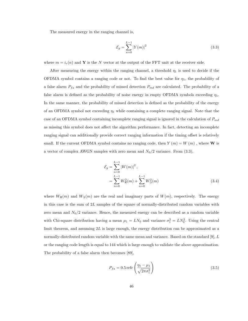
The measured energy in the ranging channel is,
Eg =
L−1∑
n=0
|Y (m)|2 (3.3)
where m = ir(n) and Y is the N vector at the output of the FFT unit at the receiver side.
After measuring the energy within the ranging channel, a threshold η1 is used to decide if the
OFDMA symbol contains a ranging code or not. To find the best value for η1, the probability of
a false alarm Pfa and the probability of missed detection Pmd are calculated. The probability of a
false alarm is defined as the probability of noise energy in empty OFDMA symbols exceeding η1.
In the same manner, the probability of missed detection is defined as the probability of the energy
of an OFDMA symbol not exceeding η1 while containing a complete ranging signal. Note that the
case of an OFDMA symbol containing incomplete ranging signal is ignored in the calculation of Pmd
as missing this symbol does not affect the algorithm performance. In fact, detecting an incomplete
ranging signal can additionally provide correct ranging information if the timing offset is relatively
small. If the current OFDMA symbol contains no ranging code, then Y (m) = W (m) , where W is
a vector of complex AWGN samples with zero mean and N0/2 variance. From (3.3),
Eg =L−1∑
n=0
|W (m)|2 ,
=
L−1∑
n=0
W 2<(m) +
L−1∑
n=0
W 2=(m) (3.4)
where W<(m) and W=(m) are the real and imaginary parts of W (m), respectively. The energy
in this case is the sum of 2L samples of the square of normally-distributed random variables with
zero mean and N0/2 variance. Hence, the measured energy can be described as a random variable
with Chi-square distribution having a mean µ1 = LN0 and variance σ21 = LN2
0 . Using the central
limit theorem, and assuming 2L is large enough, the energy distribution can be approximated as a
normally-distributed random variable with the same mean and variance. Based on the standard [9], L
or the ranging code length is equal to 144 which is large enough to validate the above approximation.
The probability of a false alarm then becomes [89],
Pfa = 0.5 erfc
(η1 − µ1√
2πσ21
)(3.5)
46
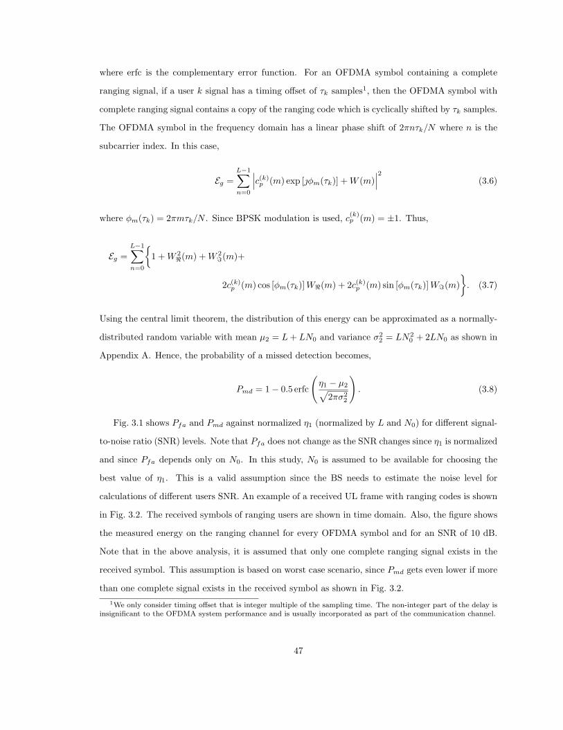
where erfc is the complementary error function. For an OFDMA symbol containing a complete
ranging signal, if a user k signal has a timing offset of τk samples1, then the OFDMA symbol with
complete ranging signal contains a copy of the ranging code which is cyclically shifted by τk samples.
The OFDMA symbol in the frequency domain has a linear phase shift of 2πnτk/N where n is the
subcarrier index. In this case,
Eg =
L−1∑
n=0
∣∣∣c(k)p (m) exp [φm(τk)] + W (m)
∣∣∣2
(3.6)
where φm(τk) = 2πmτk/N . Since BPSK modulation is used, c(k)p (m) = ±1. Thus,
Eg =L−1∑
n=0
{1 + W 2
<(m) + W 2=(m)+
2c(k)p (m) cos [φm(τk)] W<(m) + 2c(k)
p (m) sin [φm(τk)]W=(m)
}. (3.7)
Using the central limit theorem, the distribution of this energy can be approximated as a normally-
distributed random variable with mean µ2 = L + LN0 and variance σ22 = LN2
0 + 2LN0 as shown in
Appendix A. Hence, the probability of a missed detection becomes,
Pmd = 1 − 0.5 erfc
(η1 − µ2√
2πσ22
). (3.8)
Fig. 3.1 shows Pfa and Pmd against normalized η1 (normalized by L and N0) for different signal-
to-noise ratio (SNR) levels. Note that Pfa does not change as the SNR changes since η1 is normalized
and since Pfa depends only on N0. In this study, N0 is assumed to be available for choosing the
best value of η1. This is a valid assumption since the BS needs to estimate the noise level for
calculations of different users SNR. An example of a received UL frame with ranging codes is shown
in Fig. 3.2. The received symbols of ranging users are shown in time domain. Also, the figure shows
the measured energy on the ranging channel for every OFDMA symbol and for an SNR of 10 dB.
Note that in the above analysis, it is assumed that only one complete ranging signal exists in the
received symbol. This assumption is based on worst case scenario, since Pmd gets even lower if more
than one complete signal exists in the received symbol as shown in Fig. 3.2.
1We only consider timing offset that is integer multiple of the sampling time. The non-integer part of the delay isinsignificant to the OFDMA system performance and is usually incorporated as part of the communication channel.
47

0 5 10 15 20 25 30 35 400
0.1
0.2
0.3
0.4
0.5
0.6
0.7
0.8
0.9
1
Normalized Threshold η1(2/LN0)
Pro
bability
Pfa
Pmd, SNR = 0 dBPmd, SNR = 5 dBPmd, SNR = 10 dB
Figure 3.1 Pfa and Pmd for different noise levels.
3.4.2 Timing Offset Estimation
In the previous step, the system detects OFDMA symbols containing one or more complete
ranging signals. The next step is to identify how many codes are in each symbol and estimate
the timing offset for each of these codes. Since the proposed algorithm is applied in frequency
domain, timing offset would be directly translated into a linear phase shift. In this case, what is
estimated is actually the linear phase shift for each code in the current OFDMA symbol. This can
be done by cross-correlating the ranging channel of the current OFDMA symbol with all possible
codes after applying all possible linear phase shifts to the symbol. The correlator output is followed
by a threshold detector to detect different ranging codes and their phase shifts within the current
symbol. However, this is computationally complex. We intended to reduce the complexity of this
operation by exploiting the fact that timing offsets only affect the phase of the frequency domain
signal. Since BPSK modulation is used, the signal should not have an imaginary part. If there are
K ranging users within the current OFDMA symbol, each user has a timing offset τk samples, where
0 < τk < τmax and τmax is the maximum RTD between the SS and the BS within the current cell.
48
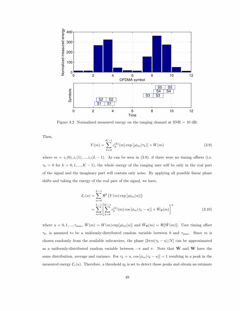
0 2 4 6 8 10 120
100
200
300
400
OFDMA symbol
Norm
aliz
ed m
easure
d e
nerg
y
0 2 4 6 8 10 12Time
Sym
bols
S1 S1S2 S2
S3 S3S4 S4S5 S5
Figure 3.2 Normalized measured energy on the ranging channel at SNR = 10 dB.
Then,
Y (m) =
K−1∑
k=0
c(k)p (m) exp [φm(τk)] + W (m) (3.9)
where m = ir(0), ir(1), ..., ir(L − 1). As can be seen in (3.9), if there were no timing offsets (i.e.
τk = 0 for k = 0, 1, ...,K − 1), the whole energy of the ranging user will be only in the real part
of the signal and the imaginary part will contain only noise. By applying all possible linear phase
shifts and taking the energy of the real part of the signal, we have,
Er(u) =
L−1∑
n=0
<2 {Y (m) exp [φm(u)]}
=
L−1∑
n=0
[K−1∑
k=0
c(k)p (m) cos [φm(τk − u)] + W<(m)
]2(3.10)
where u = 0, 1, ..., τmax, W (m) = W (m) exp[φm(u)] and W<(m) = <{W (m)}. User timing offset
τk, is assumed to be a uniformly-distributed random variable between 0 and τmax. Since m is
chosen randomly from the available subcarriers, the phase [2πm(τk − u)/N ] can be approximated
as a uniformly-distributed random variable between −π and π. Note that W and W have the
same distribution, average and variance. For τk = u, cos [φm(τk − u)] = 1 resulting in a peak in the
measured energy Er(u). Therefore, a threshold η2 is set to detect those peaks and obtain an estimate
49
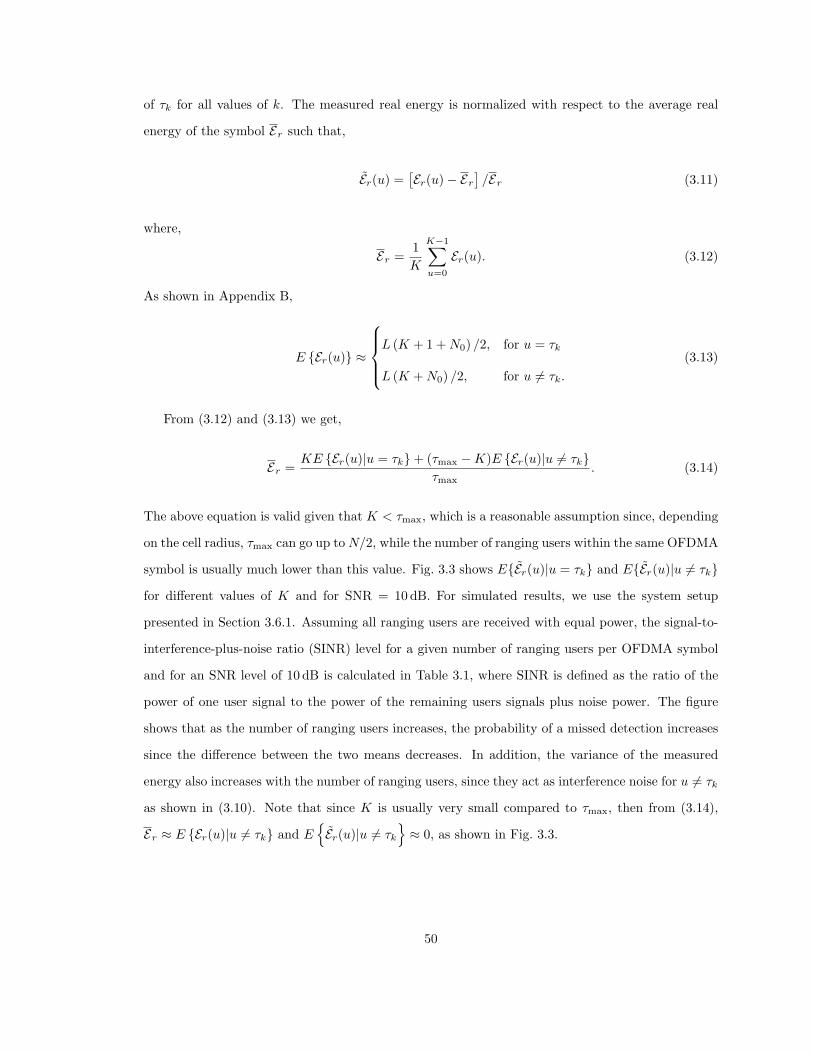
of τk for all values of k. The measured real energy is normalized with respect to the average real
energy of the symbol Er such that,
Er(u) =[Er(u) − Er
]/Er (3.11)
where,
Er =1
K
K−1∑
u=0
Er(u). (3.12)
As shown in Appendix B,
E {Er(u)} ≈
L (K + 1 + N0) /2, for u = τk
L (K + N0) /2, for u 6= τk.
(3.13)
From (3.12) and (3.13) we get,
Er =KE {Er(u)|u = τk} + (τmax − K)E {Er(u)|u 6= τk}
τmax. (3.14)
The above equation is valid given that K < τmax, which is a reasonable assumption since, depending
on the cell radius, τmax can go up to N/2, while the number of ranging users within the same OFDMA
symbol is usually much lower than this value. Fig. 3.3 shows E{Er(u)|u = τk} and E{Er(u)|u 6= τk}
for different values of K and for SNR = 10 dB. For simulated results, we use the system setup
presented in Section 3.6.1. Assuming all ranging users are received with equal power, the signal-to-
interference-plus-noise ratio (SINR) level for a given number of ranging users per OFDMA symbol
and for an SNR level of 10 dB is calculated in Table 3.1, where SINR is defined as the ratio of the
power of one user signal to the power of the remaining users signals plus noise power. The figure
shows that as the number of ranging users increases, the probability of a missed detection increases
since the difference between the two means decreases. In addition, the variance of the measured
energy also increases with the number of ranging users, since they act as interference noise for u 6= τk
as shown in (3.10). Note that since K is usually very small compared to τmax, then from (3.14),
Er ≈ E {Er(u)|u 6= τk} and E{Er(u)|u 6= τk
}≈ 0, as shown in Fig. 3.3.
50
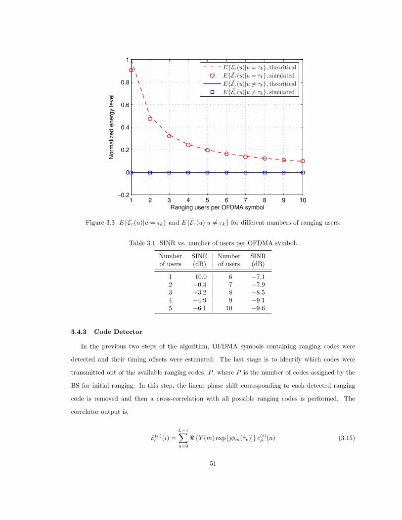
1 2 3 4 5 6 7 8 9 10−0.2
0
0.2
0.4
0.6
0.8
1
Ranging users per OFDMA symbol
Norm
aliz
ed e
nerg
y level
E{Er(u)|u = τk}, theoritical
E{Er(u)|u = τk}, simulated
E{Er(u)|u 6= τk}, theoritical
E{Er(u)|u 6= τk}, simulated
Figure 3.3 E{Er(u)|u = τk} and E{Er(u)|u 6= τk} for different numbers of ranging users.
Table 3.1 SINR vs. number of users per OFDMA symbol.
Numberof users
SINR(dB)
Numberof users
SINR(dB)
1 10.0 6 −7.12 −0.4 7 −7.93 −3.2 8 −8.54 −4.9 9 −9.15 −6.1 10 −9.6
3.4.3 Code Detector
In the previous two steps of the algorithm, OFDMA symbols containing ranging codes were
detected and their timing offsets were estimated. The last stage is to identify which codes were
transmitted out of the available ranging codes, P , where P is the number of codes assigned by the
BS for initial ranging. In this step, the linear phase shift corresponding to each detected ranging
code is removed and then a cross-correlation with all possible ranging codes is performed. The
correlator output is,
E(v)c (i) =
L−1∑
n=0
<{Y (m) exp [φm(τv)]} c(i)p (n) (3.15)
51
where i = 0, 1, ..., P − 1, and τv is the estimated timing offset of the vth user. The vector E(v)c is
calculated for every detected ranging code, v, where v = 0, 1, ..., K − 1, and K is the total number
of detected ranging codes in the second step. E(v)c is then compared to a threshold, η3, to identify
which ranging code is within the current OFDMA symbol. Note that η3 is normalized by the root
mean square value of E(v)c . Since this step should not be reached unless at least one ranging code
exists in the current OFDMA symbol, the code with maximum correlation could just be chosen
for every value of v. However, a threshold is used so that the algorithm can detect multiple codes
with the same timing offset which would be interpreted as a single code in the second step of the
algorithm. In this case, K is updated to reflect the increase in the number of detected ranging codes.
In addition, if two users happen to use the same ranging code and both their signals are received
in the same symbol but with different timing offsets, the system declares a collision and both codes
are dropped. The corresponding users then have to retry in the next available ranging opportunity.
3.5 Computational Complexity
For practical applications, the computational complexity of an algorithm is important. In this
section, we evaluate the complexity of the proposed algorithm and compare it to other algorithms.
The proposed algorithm is compared with the two proposed algorithms in [83] and [84], which
are referred to as algorithm 1 and algorithm 2, respectively. For algorithm 1, an observation window
with the OFDMA symbol size is used. A bank of correlators, equal to the number of available
ranging codes P , is used to separate ranging codes in the received signal. If the maximum possible
delay is τmax, then (τmax +1)P cross-correlation operations are performed for every OFDMA symbol
with ranging opportunity. Assuming the current UL consists of NUL OFDMA symbols, where NUL
is required by the standard to be an integer multiple of 3, then the total number of correlation
operations performed would be NUL(τmax+1)P . The same number applies for threshold comparison
operations. Algorithm 2, on the other hand, performs the cross-correlation in frequency domain.
Thus, to perform the cross-correlation at every possible timing offset, a linear phase shift of φm(u)
where u = 0, 1, ..., τmax, is applied to the frequency domain signal prior to the cross-correlators bank.
As a result, algorithm 2 has an addition of τmax + 1 linear phase shifts added to its computational
complexity. However, since the correlation is performed in the frequency domain, and since BPSK
modulation is used, the correlations are done on real-signals unlike algorithm 1 which has to perform
complex-signal correlations.
52
In the proposed algorithm, the energy of the ranging channel for every OFDMA symbol is
calculated. As a result, NUL energy calculation operations and threshold comparisons are needed.
The energy calculation is already performed for N0 estimation. Assuming that every ranging symbol
triggers the energy detector over two OFDMA symbols, then at most 2K OFDMA symbols will reach
the next stage of the algorithm, where K is the total number of ranging users within the current UL
frame. Of course, if one or more codes collide, then less OFDMA symbols will reach the next stage.
In the second stage, all possible linear phase shifts are applied to the OFDMA symbol (i.e. from 0
to τmax). The energy of the real part of the signal is measured and compared to a threshold. Thus,
(1 + τmax) linear phase shifts, real energy calculation, and comparison operations are performed. A
maximum of K ranging codes, within 2K ranging OFDMA symbols, will reach the third and last
stage. A cross-correlation with all possible codes is performed. As a result, 2KP correlations and
comparison operations (CMPs) are performed at this stage.
Table 3.2 shows the number of additions (ADDs) and multiplications (MULs) needed for each
operation. Using Table 3.2, the computational complexity of the algorithms under investigation is,
• Algorithm 1:
NULP (τmax + 1)(4L − 2) ADD + 4LNULP (τmax + 1) MUL + NULP (τmax + 1) CMP
• Algorithm 2:
(τmax + 1)(2L + NULPL − NULP ) ADD+
L(τmax + 1)(4 + NULP ) MUL + NULP (τmax + 1) CMP
• Proposed Algorithm:
[NUL(4L − 2) + 2K(τmax + 1)(3L − 1) + 2KP (L − 1)
]ADD+
[2L(KP + 2) + 10KL(τmax + 1)
]MUL +
[NUL + 2K(τmax + P + 1)
]CMP
Finally, the complexity of all three algorithms is calculated for a practical system2. We assume
NUL = 12 OFDMA symbols, P = 256 codes (maximum), L = 144 bits (standard-based [9]), and
2Using CPU cycle counts based on XilinX DSP48 slice.
53
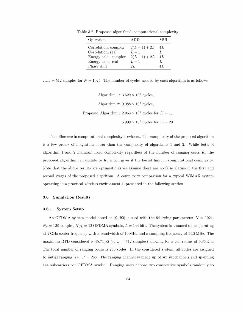
Table 3.2 Proposed algorithm’s computational complexity.
Operation ADD MUL
Correlation, complex 2(L − 1) + 2L 4LCorrelation, real L − 1 LEnergy calc., complex 2(L − 1) + 2L 4LEnergy calc., real L − 1 LPhase shift 2L 4L
τmax = 512 samples for N = 1024. The number of cycles needed by each algorithm is as follows,
Algorithm 1: 3.629 × 10⁹ cycles,
Algorithm 2: 9.088 × 10⁸ cycles,
Proposed Algorithm : 2.963 × 10⁶ cycles for K = 1,
5.909 × 10⁷ cycles for K = 20.
The difference in computational complexity is evident. The complexity of the proposed algorithm
is a few orders of magnitude lower than the complexity of algorithms 1 and 2. While both of
algorithm 1 and 2 maintain fixed complexity regardless of the number of ranging users K, the
proposed algorithm can update to K, which gives it the lowest limit in computational complexity.
Note that the above results are optimistic as we assume there are no false alarms in the first and
second stages of the proposed algorithm. A complexity comparison for a typical WiMAX system
operating in a practical wireless environment is presented in the following section.
3.6 Simulation Results
3.6.1 System Setup
An OFDMA system model based on [9, 90] is used with the following parameters: N = 1024,
Ng = 128 samples, NUL = 12 OFDMA symbols, L = 144 bits. The system is assumed to be operating
at 2 GHz center frequency with a bandwidth of 10 MHz and a sampling frequency of 11.2 MHz. The
maximum RTD considered is 45.71 µS (τmax = 512 samples) allowing for a cell radius of 6.86 Km.
The total number of ranging codes is 256 codes. In the considered system, all codes are assigned
to initial ranging, i.e. P = 256. The ranging channel is made up of six subchannels and spanning
144 subcarriers per OFDMA symbol. Ranging users choose two consecutive symbols randomly to
54
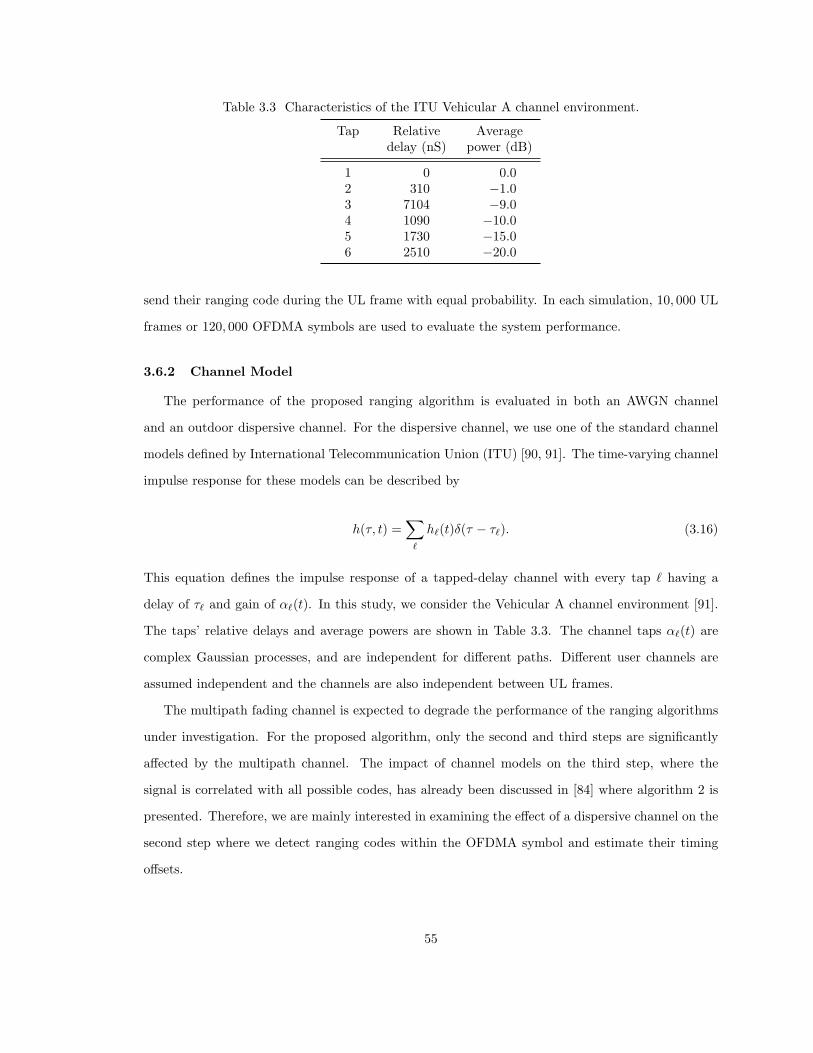
Table 3.3 Characteristics of the ITU Vehicular A channel environment.
Tap Relativedelay (nS)
Averagepower (dB)
1 0 0.02 310 −1.03 7104 −9.04 1090 −10.05 1730 −15.06 2510 −20.0
send their ranging code during the UL frame with equal probability. In each simulation, 10, 000 UL
frames or 120, 000 OFDMA symbols are used to evaluate the system performance.
3.6.2 Channel Model
The performance of the proposed ranging algorithm is evaluated in both an AWGN channel
and an outdoor dispersive channel. For the dispersive channel, we use one of the standard channel
models defined by International Telecommunication Union (ITU) [90, 91]. The time-varying channel
impulse response for these models can be described by
h(τ, t) =∑
`
h`(t)δ(τ − τ`). (3.16)
This equation defines the impulse response of a tapped-delay channel with every tap ` having a
delay of τ` and gain of α`(t). In this study, we consider the Vehicular A channel environment [91].
The taps’ relative delays and average powers are shown in Table 3.3. The channel taps α`(t) are
complex Gaussian processes, and are independent for different paths. Different user channels are
assumed independent and the channels are also independent between UL frames.
The multipath fading channel is expected to degrade the performance of the ranging algorithms
under investigation. For the proposed algorithm, only the second and third steps are significantly
affected by the multipath channel. The impact of channel models on the third step, where the
signal is correlated with all possible codes, has already been discussed in [84] where algorithm 2 is
presented. Therefore, we are mainly interested in examining the effect of a dispersive channel on the
second step where we detect ranging codes within the OFDMA symbol and estimate their timing
offsets.
55
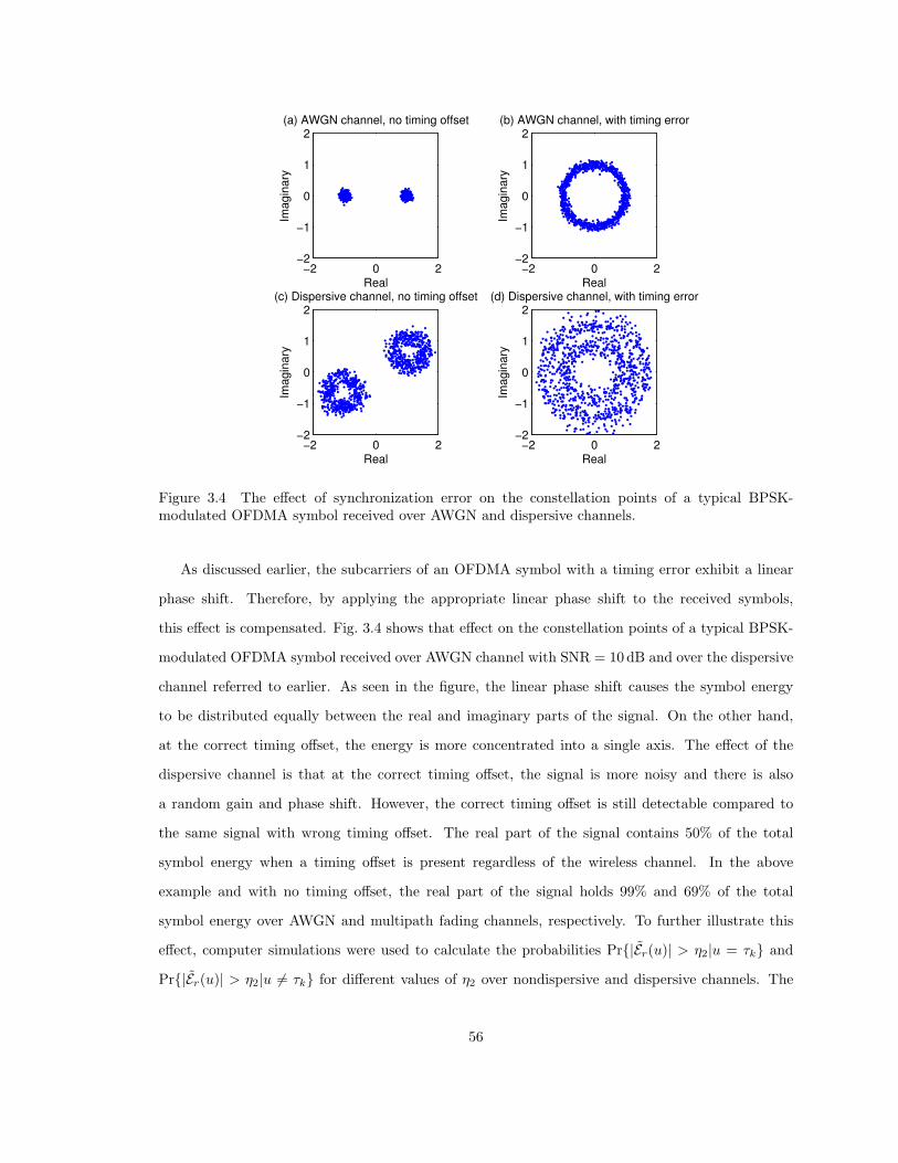
−2 0 2−2
−1
0
1
2(a) AWGN channel, no timing offset
RealIm
agin
ary
−2 0 2−2
−1
0
1
2(b) AWGN channel, with timing error
Real
Imagin
ary
−2 0 2−2
−1
0
1
2(c) Dispersive channel, no timing offset
Real
Imagin
ary
−2 0 2−2
−1
0
1
2(d) Dispersive channel, with timing error
Real
Imagin
ary
Figure 3.4 The effect of synchronization error on the constellation points of a typical BPSK-modulated OFDMA symbol received over AWGN and dispersive channels.
As discussed earlier, the subcarriers of an OFDMA symbol with a timing error exhibit a linear
phase shift. Therefore, by applying the appropriate linear phase shift to the received symbols,
this effect is compensated. Fig. 3.4 shows that effect on the constellation points of a typical BPSK-
modulated OFDMA symbol received over AWGN channel with SNR = 10 dB and over the dispersive
channel referred to earlier. As seen in the figure, the linear phase shift causes the symbol energy
to be distributed equally between the real and imaginary parts of the signal. On the other hand,
at the correct timing offset, the energy is more concentrated into a single axis. The effect of the
dispersive channel is that at the correct timing offset, the signal is more noisy and there is also
a random gain and phase shift. However, the correct timing offset is still detectable compared to
the same signal with wrong timing offset. The real part of the signal contains 50% of the total
symbol energy when a timing offset is present regardless of the wireless channel. In the above
example and with no timing offset, the real part of the signal holds 99% and 69% of the total
symbol energy over AWGN and multipath fading channels, respectively. To further illustrate this
effect, computer simulations were used to calculate the probabilities Pr{|Er(u)| > η2|u = τk} and
Pr{|Er(u)| > η2|u 6= τk} for different values of η2 over nondispersive and dispersive channels. The
56
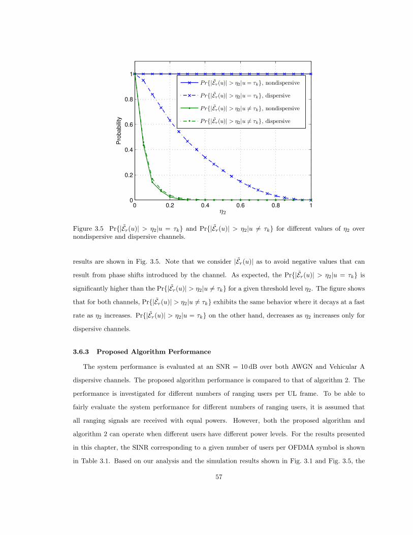
0 0.2 0.4 0.6 0.8 10
0.2
0.4
0.6
0.8
1
η2
Pro
ba
bili
ty
Pr{|Er(u)| > η2|u = τk}, nondispersive
Pr{|Er(u)| > η2|u = τk}, dispersive
Pr{|Er(u)| > η2|u 6= τk}, nondispersive
Pr{|Er(u)| > η2|u 6= τk}, dispersive
Figure 3.5 Pr{|Er(u)| > η2|u = τk} and Pr{|Er(u)| > η2|u 6= τk} for different values of η2 overnondispersive and dispersive channels.
results are shown in Fig. 3.5. Note that we consider |Er(u)| as to avoid negative values that can
result from phase shifts introduced by the channel. As expected, the Pr{|Er(u)| > η2|u = τk} is
significantly higher than the Pr{|Er(u)| > η2|u 6= τk} for a given threshold level η2. The figure shows
that for both channels, Pr{|Er(u)| > η2|u 6= τk} exhibits the same behavior where it decays at a fast
rate as η2 increases. Pr{|Er(u)| > η2|u = τk} on the other hand, decreases as η2 increases only for
dispersive channels.
3.6.3 Proposed Algorithm Performance
The system performance is evaluated at an SNR = 10 dB over both AWGN and Vehicular A
dispersive channels. The proposed algorithm performance is compared to that of algorithm 2. The
performance is investigated for different numbers of ranging users per UL frame. To be able to
fairly evaluate the system performance for different numbers of ranging users, it is assumed that
all ranging signals are received with equal powers. However, both the proposed algorithm and
algorithm 2 can operate when different users have different power levels. For the results presented
in this chapter, the SINR corresponding to a given number of users per OFDMA symbol is shown
in Table 3.1. Based on our analysis and the simulation results shown in Fig. 3.1 and Fig. 3.5, the
57

1 2 3 4 5 6 7 8 9 100
0.05
0.1
0.15
0.2
0.25
0.3
0.35
Number of ranging users per UL frame
Pro
ba
bili
ty o
f m
isse
d d
ete
ctio
n
Proposed alg., dispersive
Alg. 2, dispersive
Proposed alg., AWGN
Alg. 2, AWGN
Figure 3.6 Probability of missed detection.
thresholds (η1, η2, η3) for the proposed algorithm are chosen to be (3, 0.2, 6) for AWGN channels
and (3, 0.1, 6) for dispersive channels. Fig. 3.6 and Fig. 3.7 show the probability of missed detection
and the probability of false alarm, respectively, for both the proposed algorithm and algorithm 2,
and for different numbers of ranging users per UL frame. Over AWGN channels, both algorithm
performances are almost identical with zero probability of false alarm. Over dispersive channels,
the proposed algorithm suffers from a higher probability of missed detection compared to algorithm
2. The difference between the two algorithms increases as the number of users increases. On the
other hand, the proposed algorithm shows a much lower probability of false alarm than algorithm
2 especially for low number of ranging users. Even with up to 8 ranging users per UL frame, the
proposed algorithm is able to detect more than 75% of received codes with a false alarm probability
less than 0.2%.
An important measure of the ranging algorithm quality is the timing estimation accuracy. For
dispersive channels, the timing error definition is ambiguous [81]. In this study, we consider the
timing error relative to the channel tap with maximum average power, or first tap in the considered
dispersive channel. The standard deviations for the timing estimator errors for both the proposed
algorithm and algorithm 2 are shown in Fig. 3.8. Both algorithms show zero timing errors for AWGN
58
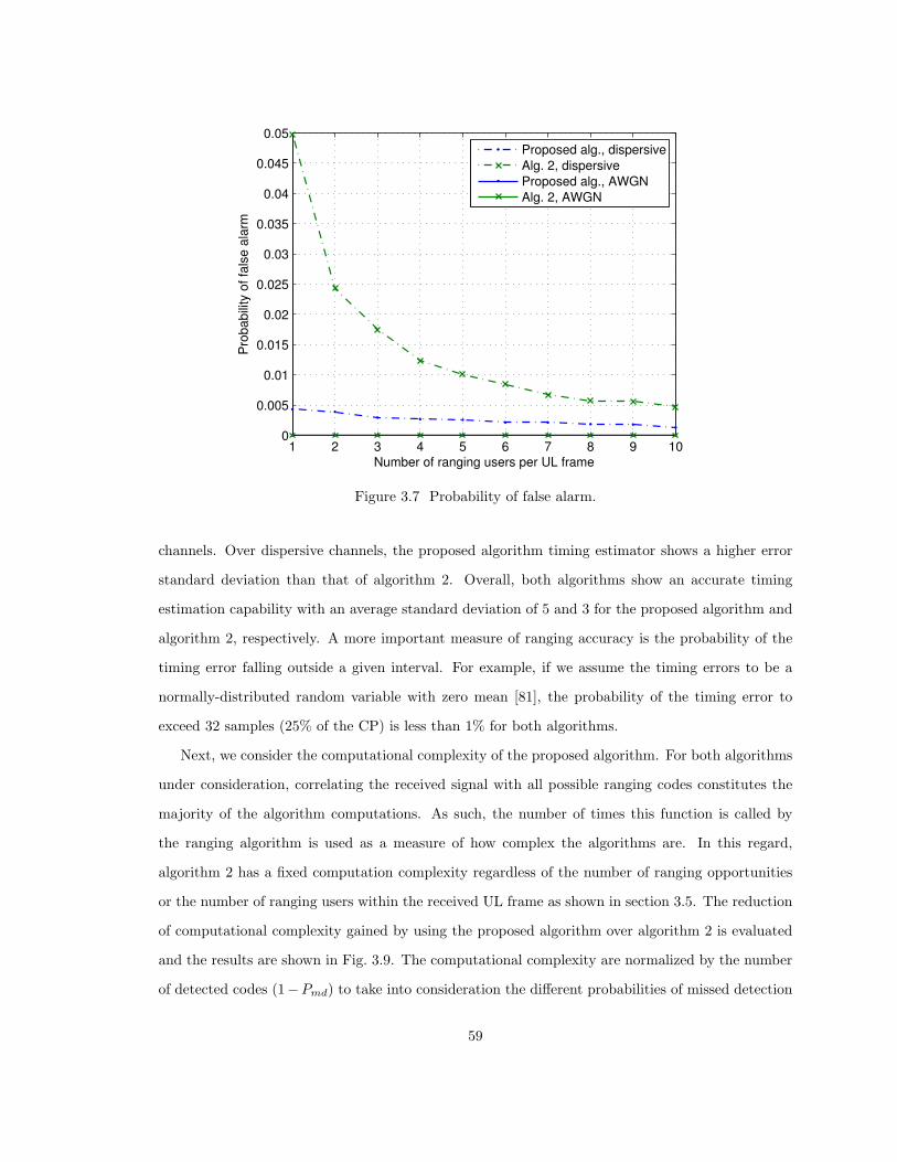
1 2 3 4 5 6 7 8 9 100
0.005
0.01
0.015
0.02
0.025
0.03
0.035
0.04
0.045
0.05
Number of ranging users per UL frame
Pro
ba
bili
ty o
f fa
lse
ala
rm
Proposed alg., dispersive
Alg. 2, dispersive
Proposed alg., AWGN
Alg. 2, AWGN
Figure 3.7 Probability of false alarm.
channels. Over dispersive channels, the proposed algorithm timing estimator shows a higher error
standard deviation than that of algorithm 2. Overall, both algorithms show an accurate timing
estimation capability with an average standard deviation of 5 and 3 for the proposed algorithm and
algorithm 2, respectively. A more important measure of ranging accuracy is the probability of the
timing error falling outside a given interval. For example, if we assume the timing errors to be a
normally-distributed random variable with zero mean [81], the probability of the timing error to
exceed 32 samples (25% of the CP) is less than 1% for both algorithms.
Next, we consider the computational complexity of the proposed algorithm. For both algorithms
under consideration, correlating the received signal with all possible ranging codes constitutes the
majority of the algorithm computations. As such, the number of times this function is called by
the ranging algorithm is used as a measure of how complex the algorithms are. In this regard,
algorithm 2 has a fixed computation complexity regardless of the number of ranging opportunities
or the number of ranging users within the received UL frame as shown in section 3.5. The reduction
of computational complexity gained by using the proposed algorithm over algorithm 2 is evaluated
and the results are shown in Fig. 3.9. The computational complexity are normalized by the number
of detected codes (1−Pmd) to take into consideration the different probabilities of missed detection
59
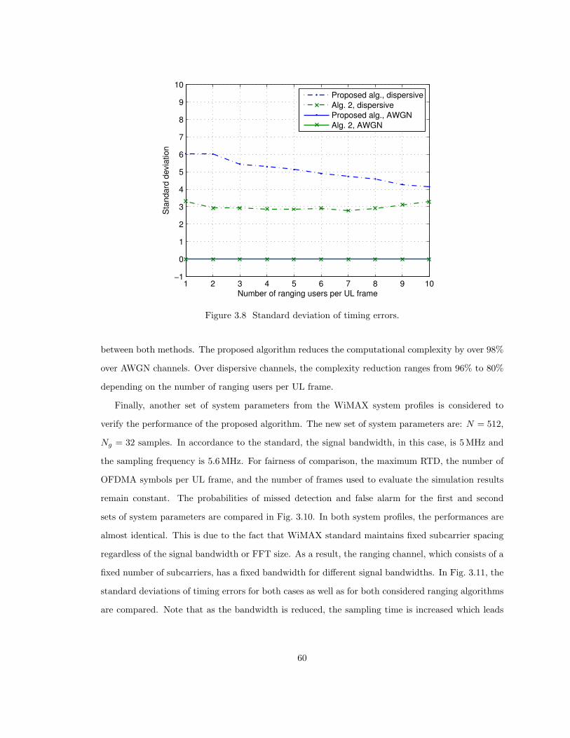
1 2 3 4 5 6 7 8 9 10−1
0
1
2
3
4
5
6
7
8
9
10
Number of ranging users per UL frame
Sta
nd
ard
de
via
tio
n
Proposed alg., dispersive
Alg. 2, dispersive
Proposed alg., AWGN
Alg. 2, AWGN
Figure 3.8 Standard deviation of timing errors.
between both methods. The proposed algorithm reduces the computational complexity by over 98%
over AWGN channels. Over dispersive channels, the complexity reduction ranges from 96% to 80%
depending on the number of ranging users per UL frame.
Finally, another set of system parameters from the WiMAX system profiles is considered to
verify the performance of the proposed algorithm. The new set of system parameters are: N = 512,
Ng = 32 samples. In accordance to the standard, the signal bandwidth, in this case, is 5 MHz and
the sampling frequency is 5.6 MHz. For fairness of comparison, the maximum RTD, the number of
OFDMA symbols per UL frame, and the number of frames used to evaluate the simulation results
remain constant. The probabilities of missed detection and false alarm for the first and second
sets of system parameters are compared in Fig. 3.10. In both system profiles, the performances are
almost identical. This is due to the fact that WiMAX standard maintains fixed subcarrier spacing
regardless of the signal bandwidth or FFT size. As a result, the ranging channel, which consists of a
fixed number of subcarriers, has a fixed bandwidth for different signal bandwidths. In Fig. 3.11, the
standard deviations of timing errors for both cases as well as for both considered ranging algorithms
are compared. Note that as the bandwidth is reduced, the sampling time is increased which leads
60
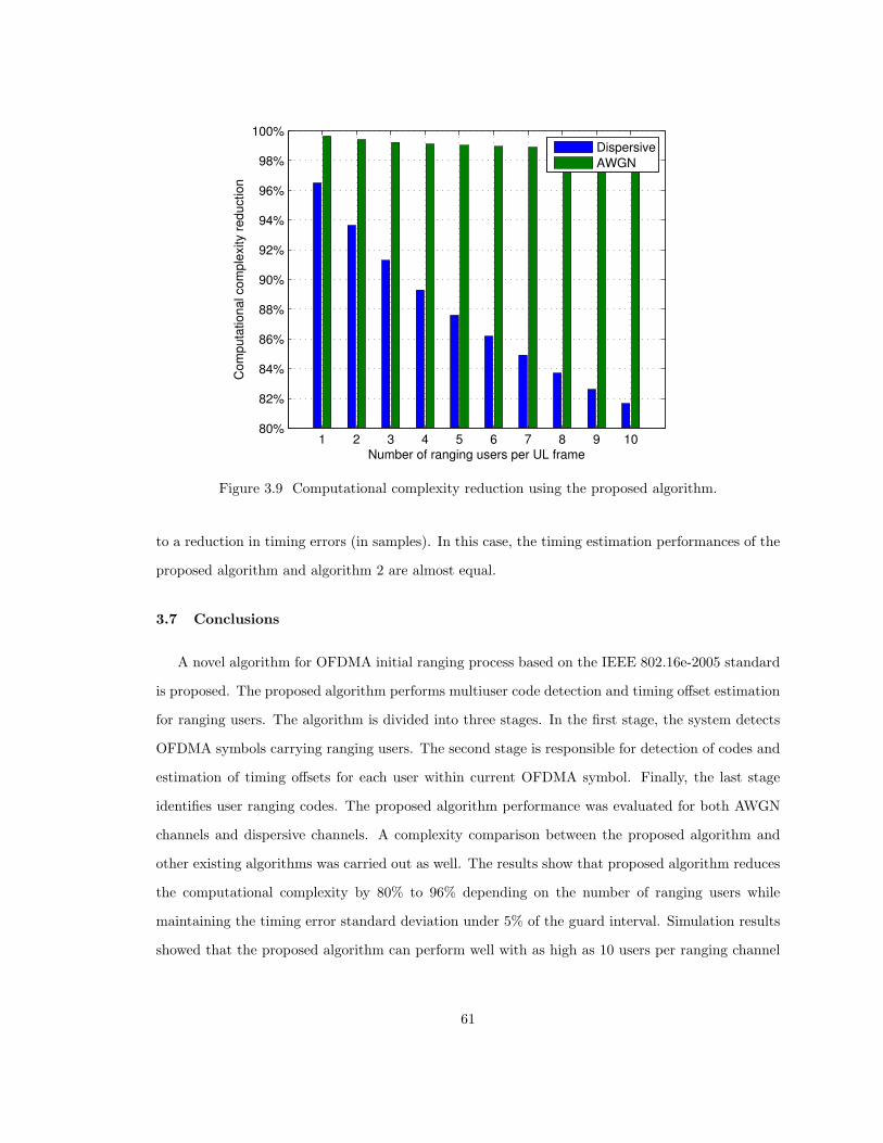
1 2 3 4 5 6 7 8 9 10 80%
82%
84%
86%
88%
90%
92%
94%
96%
98%
100%
Number of ranging users per UL frame
Co
mp
uta
tio
na
l co
mp
lexity r
ed
uctio
n
Dispersive
AWGN
Figure 3.9 Computational complexity reduction using the proposed algorithm.
to a reduction in timing errors (in samples). In this case, the timing estimation performances of the
proposed algorithm and algorithm 2 are almost equal.
3.7 Conclusions
A novel algorithm for OFDMA initial ranging process based on the IEEE 802.16e-2005 standard
is proposed. The proposed algorithm performs multiuser code detection and timing offset estimation
for ranging users. The algorithm is divided into three stages. In the first stage, the system detects
OFDMA symbols carrying ranging users. The second stage is responsible for detection of codes and
estimation of timing offsets for each user within current OFDMA symbol. Finally, the last stage
identifies user ranging codes. The proposed algorithm performance was evaluated for both AWGN
channels and dispersive channels. A complexity comparison between the proposed algorithm and
other existing algorithms was carried out as well. The results show that proposed algorithm reduces
the computational complexity by 80% to 96% depending on the number of ranging users while
maintaining the timing error standard deviation under 5% of the guard interval. Simulation results
showed that the proposed algorithm can perform well with as high as 10 users per ranging channel
61

1 2 3 4 5 6 7 8 9 100
0.05
0.1
0.15
0.2
0.25
0.3
0.35
Number of ranging users per UL frame
Pro
ba
bili
ty
Probability of missed detection, N=512
Probability of missed detection, N=1024
Probability of false alarm, N=512
Probability of false alarm, N=1024
Figure 3.10 Probabilities of missed detection and false alarm for N = 1024 and N = 512.
in a given UL frame. Hence, it is believed that the proposed algorithm can be realized in practical
OFDMA-based BSs.
62
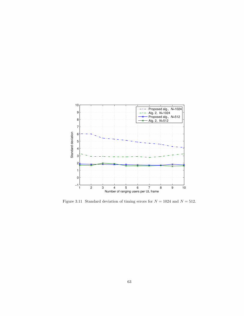
1 2 3 4 5 6 7 8 9 10−1
0
1
2
3
4
5
6
7
8
9
10
Number of ranging users per UL frame
Sta
nd
ard
de
via
tio
n
Proposed alg., N=1024
Alg. 2, N=1024
Proposed alg., N=512
Alg. 2, N=512
Figure 3.11 Standard deviation of timing errors for N = 1024 and N = 512.
63
CHAPTER 4
SPECTRUM SHAPING OF OFDM-BASED COGNITIVE RADIO SIGNALS
4.1 Introduction
Recently, opportunistic usage of licensed frequency bands has been proposed as a solution to
spectral crowding problem by using cognitive radio (CR) systems [2, 60]. A CR system would
be able to operate in licensed bands by utilizing vacant parts of these bands. A key point for
the success of CR is the ability to shape its signal spectrum to achieve minimum interference to
licensed users (LU). Orthogonal frequency division multiplexing (OFDM) has been proposed as
a candidate signaling technology for such applications. By dividing the spectrum into subbands
that are modulated with orthogonal subcarriers, OFDM spectrum can be shaped with more ease
compared to other signaling techniques. However, modulated OFDM subcarriers suffer from high
sidelobes, which result in adjacent channel interference (ACI). Thus, disabling a set of OFDM
subcarriers to create a spectrum null may not be sufficient to avoid interference to LU. On the other
hand, using filters can increase the system complexity and introduce long delays. Using guard bands
on both sides of used OFDM spectrum and windowing the time domain signal have been investigated
in [64]. In [65–67], the use of interference cancellation carriers (CC) is proposed. Other proposed
methods include the use of subcarrier weighting [74] or multiple-choice sequences [75].
In this chapter, we discuss some of the current methods and techniques proposed in the literature
for spectrum shaping of an OFDM signal to avoid or minimize interference to LUs. We investigate
the effect of various system parameters (such as the LU bandwidth, cyclic prefix (CP) length,
and number of CCs) and their effects on the system performance in terms of interference level,
spectral efficiency, computational complexity, and power consumption. Simulation results showing
the system performance are provided along with discussions of the advantages and disadvantages of
each technique. We then propose a new method, referred to as adaptive symbol transition (AST),
to suppress OFDM sidelobes and shape the signal spectrum. Similar to the windowing technique,
64
the OFDM symbols are extended in time to reduce the effect of symbol transition. However, instead
of using a predefined filter shape, the transition signal is optimized adaptively based on transmitted
data and detected LU bands to reduce the interference to LUs.
4.2 System Model
Throughout this chapter, we assume a CR system employing OFDM as the signaling technique.
The CR is assumed to be aware of the surrounding environment and the radio channel characteristics.
After scanning the channel, the CR should be able to identify LUs operating within the targeted
band [92]. The goal is to exploit identified spectrum opportunities and achieve highest possible
spectral efficiency while keeping the interference to detected LUs to minimum. In the system, the
encoded data is modulated and then fed to an N -point inverse fast Fourier transform (IFFT) unit.
We define FN1,N2= {Fn1,n2
} as the N1-point Fourier transform matrix of a vector of length N2,
where
Fn1,n2= exp
(−j2πn1n2
N1
). (4.1)
The time domain signal at the output of the IFFT is
x =1
NF∗
N,NX, (4.2)
where N is the IFFT size, (·)∗ is the complex conjugate operator, 1N F∗ is the inverse Fourier
transform matrix, and X = [X(1),X(2), ...,X(N)]T is the modulated data vector. The signal is
then extended using a CP consisting of Ng samples. The signal goes through a pulse shaping filter
before being sent through the communication channel.
4.3 Active Cancellation Carriers
Active CCs technique was proposed in [65–67] where a few tones at both edges of the spectrum
hole are used to cancel the interference to LUs. First, we start by examining the performance of
CCs with no cyclic extension or pulse shaping used to simplify the analysis. However, the effect of
CP is discussed later in Section 4.3. The time domain signal is upsampled by a factor of ζ and the
signal spectrum is calculated as follows
S = FζN×Nx = QX, (4.3)
65
where
Q =1
NFζN×NF∗
N×N . (4.4)
Note that ζ corresponds also to the number of points per sidelobe that are considered in the spectrum
shaping process. Unless otherwise mentioned, the value of ζ is set to eight. A LU is detected within
the OFDM band spanning over B subcarriers X(i + 1),X(i + 2), ...,X(i + B), where i∆f is the LU
signal offset with respect to the OFDM signal, B∆f is the LU signal bandwidth, and ∆f is the
frequency subcarrier separation. If the above subcarriers are disabled and remaining subcarriers are
used for data transmission, the interference to LU band is
IL = QBXB , (4.5)
where QB is a subset of Q containing only the rows of Q that corresponds to the LU band, ζ(i + 1)
to ζ(i + B), and XB is the same as X but with interference subcarriers, X(i + 1) to X(i + B), set
to zero. Assume c CCs on each edge of the spectrum gap are used to cancel the interference to LU
band. In this case, subcarriers X(i + 1 − c) to X(i + B + c) are set to zero in XB to measure the
interference to LU band. With the use of CCs, interference power to LU is,
PI =‖ QIXI + IL ‖2 . (4.6)
where QI is a subset of QB containing only the columns corresponding to disabled subcarriers,
i + 1 − c to i + B + c, and XI is a vector of required values of disabled subcarriers to minimize the
interference. The mean-squared-error (MSE) solution to the above equation is,
XI = −(QHI QI)−1QH
I IL, (4.7)
where (·)H is the Hermitian transpose. From (4.5), (4.7) can be written as
XI = WIXB , (4.8)
where WI = −(QHI QI)−1QH
I QB . Note that WI needs to be calculated only once for the same
spectrum shape while XI is calculated for every OFDM symbol [65].
66
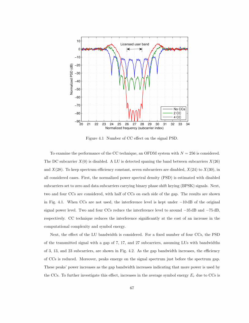
20 21 22 23 24 25 26 27 28 29 30 31 32 33 34−90
−80
−70
−60
−50
−40
−30
−20
−10
0
10
Normalized frequency (subcarrier index)
Norm
aliz
ed P
SD
(dB
)
No CCs
2 CC
4 CC
Licensed user band
Figure 4.1 Number of CC effect on the signal PSD.
To examine the performance of the CC technique, an OFDM system with N = 256 is considered.
The DC subcarrier X(0) is disabled. A LU is detected spaning the band between subcarriers X(26)
and X(28). To keep spectrum efficiency constant, seven subcarriers are disabled, X(24) to X(30), in
all considered cases. First, the normalized power spectral density (PSD) is estimated with disabled
subcarriers set to zero and data subcarriers carrying binary phase shift keying (BPSK) signals. Next,
two and four CCs are considered, with half of CCs on each side of the gap. The results are shown
in Fig. 4.1. When CCs are not used, the interference level is kept under −10 dB of the original
signal power level. Two and four CCs reduce the interference level to around −35 dB and −75 dB,
respectively. CC technique reduces the interference significantly at the cost of an increase in the
computational complexity and symbol energy.
Next, the effect of the LU bandwidth is considered. For a fixed number of four CCs, the PSD
of the transmitted signal with a gap of 7, 17, and 27 subcarriers, assuming LUs with bandwidths
of 3, 13, and 23 subcarriers, are shown in Fig. 4.2. As the gap bandwidth increases, the efficiency
of CCs is reduced. Moreover, peaks emerge on the signal spectrum just before the spectrum gap.
These peaks’ power increases as the gap bandwidth increases indicating that more power is used by
the CCs. To further investigate this effect, increases in the average symbol energy Er due to CCs is
67
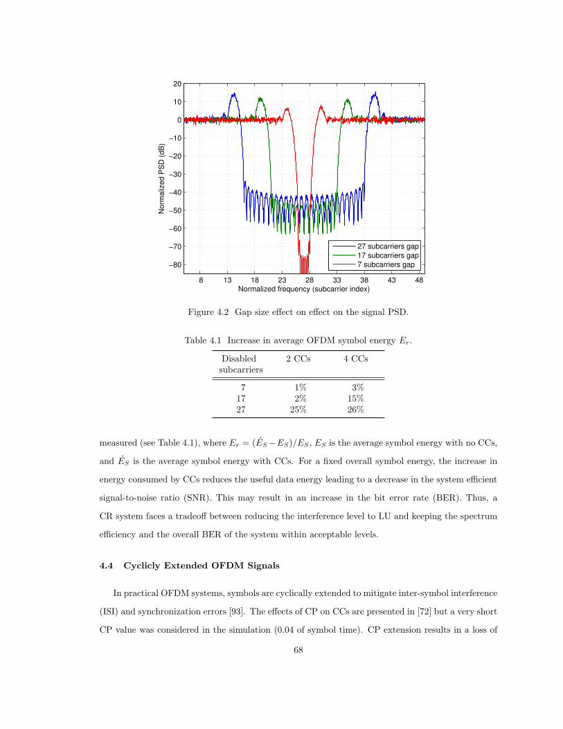
8 13 18 23 28 33 38 43 48
−80
−70
−60
−50
−40
−30
−20
−10
0
10
20
Normalized frequency (subcarrier index)
Norm
aliz
ed P
SD
(dB
)
27 subcarriers gap
17 subcarriers gap
7 subcarriers gap
Figure 4.2 Gap size effect on effect on the signal PSD.
Table 4.1 Increase in average OFDM symbol energy Er.
Disabledsubcarriers
2 CCs 4 CCs
7 1% 3%17 2% 15%27 25% 26%
measured (see Table 4.1), where Er = (ES −ES)/ES , ES is the average symbol energy with no CCs,
and ES is the average symbol energy with CCs. For a fixed overall symbol energy, the increase in
energy consumed by CCs reduces the useful data energy leading to a decrease in the system efficient
signal-to-noise ratio (SNR). This may result in an increase in the bit error rate (BER). Thus, a
CR system faces a tradeoff between reducing the interference level to LU and keeping the spectrum
efficiency and the overall BER of the system within acceptable levels.
4.4 Cyclicly Extended OFDM Signals
In practical OFDM systems, symbols are cyclically extended to mitigate inter-symbol interference
(ISI) and synchronization errors [93]. The effects of CP on CCs are presented in [72] but a very short
CP value was considered in the simulation (0.04 of symbol time). CP extension results in a loss of
68
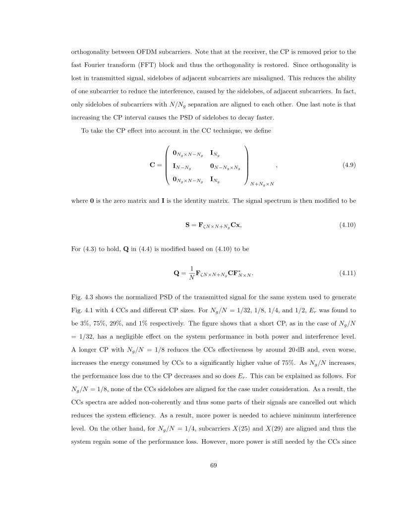
orthogonality between OFDM subcarriers. Note that at the receiver, the CP is removed prior to the
fast Fourier transform (FFT) block and thus the orthogonality is restored. Since orthogonality is
lost in transmitted signal, sidelobes of adjacent subcarriers are misaligned. This reduces the ability
of one subcarrier to reduce the interference, caused by the sidelobes, of adjacent subcarriers. In fact,
only sidelobes of subcarriers with N/Ng separation are aligned to each other. One last note is that
increasing the CP interval causes the PSD of sidelobes to decay faster.
To take the CP effect into account in the CC technique, we define
C =
0Ng×N−NgINg
IN−Ng0N−Ng×Ng
0Ng×N−NgINg
N+Ng×N
, (4.9)
where 0 is the zero matrix and I is the identity matrix. The signal spectrum is then modified to be
S = FζN×N+NgCx, (4.10)
For (4.3) to hold, Q in (4.4) is modified based on (4.10) to be
Q =1
NFζN×N+Ng
CF∗N×N . (4.11)
Fig. 4.3 shows the normalized PSD of the transmitted signal for the same system used to generate
Fig. 4.1 with 4 CCs and different CP sizes. For Ng/N = 1/32, 1/8, 1/4, and 1/2, Er was found to
be 3%, 75%, 29%, and 1% respectively. The figure shows that a short CP, as in the case of Ng/N
= 1/32, has a negligible effect on the system performance in both power and interference level.
A longer CP with Ng/N = 1/8 reduces the CCs effectiveness by around 20 dB and, even worse,
increases the energy consumed by CCs to a significantly higher value of 75%. As Ng/N increases,
the performance loss due to the CP decreases and so does Er. This can be explained as follows. For
Ng/N = 1/8, none of the CCs sidelobes are aligned for the case under consideration. As a result, the
CCs spectra are added non-coherently and thus some parts of their signals are cancelled out which
reduces the system efficiency. As a result, more power is needed to achieve minimum interference
level. On the other hand, for Ng/N = 1/4, subcarriers X(25) and X(29) are aligned and thus the
system regain some of the performance loss. However, more power is still needed by the CCs since
69
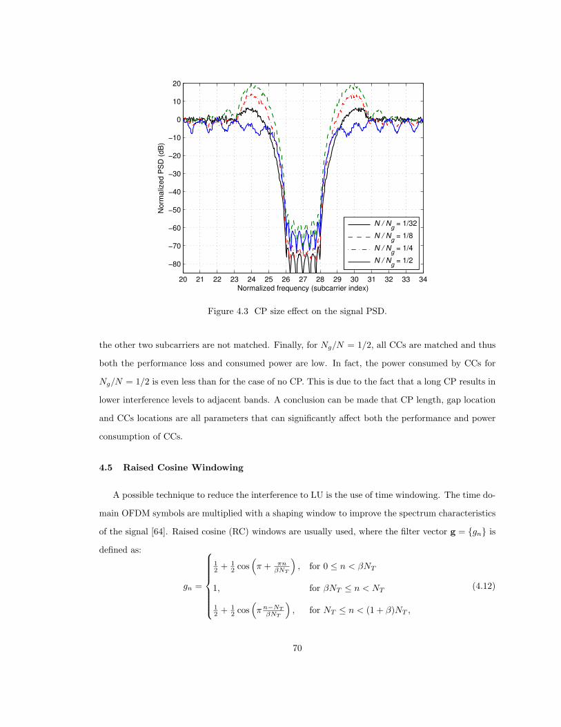
20 21 22 23 24 25 26 27 28 29 30 31 32 33 34
−80
−70
−60
−50
−40
−30
−20
−10
0
10
20
Normalized frequency (subcarrier index)
Norm
aliz
ed P
SD
(dB
)
N / Ng = 1/32
N / Ng = 1/8
N / Ng = 1/4
N / Ng = 1/2
Figure 4.3 CP size effect on the signal PSD.
the other two subcarriers are not matched. Finally, for Ng/N = 1/2, all CCs are matched and thus
both the performance loss and consumed power are low. In fact, the power consumed by CCs for
Ng/N = 1/2 is even less than for the case of no CP. This is due to the fact that a long CP results in
lower interference levels to adjacent bands. A conclusion can be made that CP length, gap location
and CCs locations are all parameters that can significantly affect both the performance and power
consumption of CCs.
4.5 Raised Cosine Windowing
A possible technique to reduce the interference to LU is the use of time windowing. The time do-
main OFDM symbols are multiplied with a shaping window to improve the spectrum characteristics
of the signal [64]. Raised cosine (RC) windows are usually used, where the filter vector g = {gn} is
defined as:
gn =
12 + 1
2 cos(π + πn
βNT
), for 0 ≤ n < βNT
1, for βNT ≤ n < NT
12 + 1
2 cos(π n−NT
βNT
), for NT ≤ n < (1 + β)NT ,
(4.12)
70
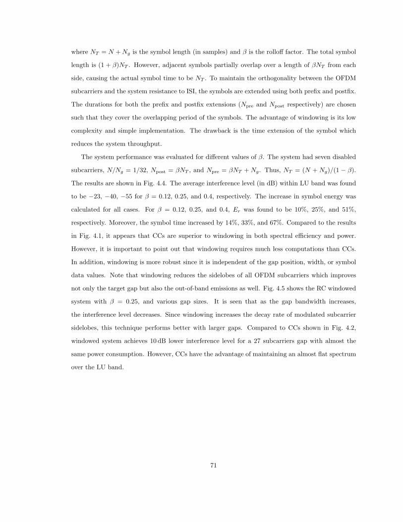
where NT = N + Ng is the symbol length (in samples) and β is the rolloff factor. The total symbol
length is (1 + β)NT . However, adjacent symbols partially overlap over a length of βNT from each
side, causing the actual symbol time to be NT . To maintain the orthogonality between the OFDM
subcarriers and the system resistance to ISI, the symbols are extended using both prefix and postfix.
The durations for both the prefix and postfix extensions (Npre and Npost respectively) are chosen
such that they cover the overlapping period of the symbols. The advantage of windowing is its low
complexity and simple implementation. The drawback is the time extension of the symbol which
reduces the system throughput.
The system performance was evaluated for different values of β. The system had seven disabled
subcarriers, N/Ng = 1/32, Npost = βNT , and Npre = βNT + Ng. Thus, NT = (N + Ng)/(1 − β).
The results are shown in Fig. 4.4. The average interference level (in dB) within LU band was found
to be −23, −40, −55 for β = 0.12, 0.25, and 0.4, respectively. The increase in symbol energy was
calculated for all cases. For β = 0.12, 0.25, and 0.4, Er was found to be 10%, 25%, and 51%,
respectively. Moreover, the symbol time increased by 14%, 33%, and 67%. Compared to the results
in Fig. 4.1, it appears that CCs are superior to windowing in both spectral efficiency and power.
However, it is important to point out that windowing requires much less computations than CCs.
In addition, windowing is more robust since it is independent of the gap position, width, or symbol
data values. Note that windowing reduces the sidelobes of all OFDM subcarriers which improves
not only the target gap but also the out-of-band emissions as well. Fig. 4.5 shows the RC windowed
system with β = 0.25, and various gap sizes. It is seen that as the gap bandwidth increases,
the interference level decreases. Since windowing increases the decay rate of modulated subcarrier
sidelobes, this technique performs better with larger gaps. Compared to CCs shown in Fig. 4.2,
windowed system achieves 10 dB lower interference level for a 27 subcarriers gap with almost the
same power consumption. However, CCs have the advantage of maintaining an almost flat spectrum
over the LU band.
71
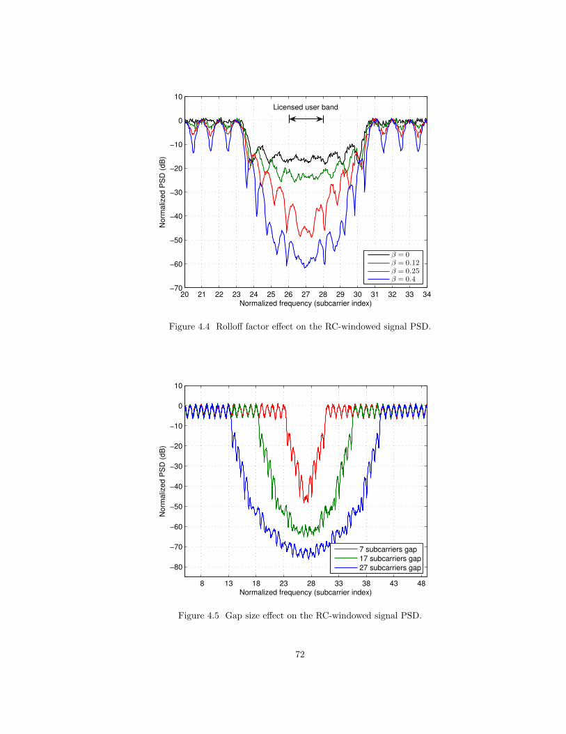
20 21 22 23 24 25 26 27 28 29 30 31 32 33 34−70
−60
−50
−40
−30
−20
−10
0
10
Normalized frequency (subcarrier index)
Norm
aliz
ed P
SD
(dB
)
β = 0β = 0.12β = 0.25β = 0.4
Licensed user band
Figure 4.4 Rolloff factor effect on the RC-windowed signal PSD.
8 13 18 23 28 33 38 43 48
−80
−70
−60
−50
−40
−30
−20
−10
0
10
Normalized frequency (subcarrier index)
Norm
aliz
ed P
SD
(dB
)
7 subcarriers gap
17 subcarriers gap
27 subcarriers gap
Figure 4.5 Gap size effect on the RC-windowed signal PSD.
72
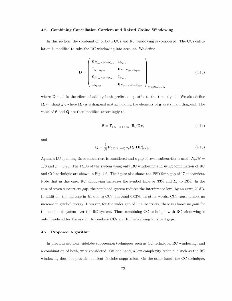
4.6 Combining Cancellation Carriers and Raised Cosine Windowing
In this section, the combination of both CCs and RC windowing is considered. The CCs calcu-
lation is modified to take the RC windowing into account. We define
D =
0Npre×N−NpreINpre
IN−Npre0N−Npre×Npre
0Npre×N−NpreINpre
INpost0Npost×N−Npost
(1+β)NT ×N
, (4.13)
where D models the effect of adding both prefix and postfix to the time signal. We also define
RC = diag{g}, where RC is a diagonal matrix holding the elements of g as its main diagonal. The
value of S and Q are then modified accordingly to
S = FζN×(1+β)NTRCDx, (4.14)
and
Q =1
NFζN×(1+β)NT
RCDF∗N×N . (4.15)
Again, a LU spanning three subcarriers is considered and a gap of seven subcarriers is used. Ng/N =
1/8 and β = 0.25. The PSDs of the system using only RC windowing and using combination of RC
and CCs technique are shown in Fig. 4.6. The figure also shows the PSD for a gap of 17 subcarriers.
Note that in this case, RC windowing increases the symbol time by 33% and Er to 13%. In the
case of seven subcarriers gap, the combined system reduces the interference level by an extra 20 dB.
In addition, the increase in Er due to CCs is around 0.02%. In other words, CCs cause almost no
increase in symbol energy. However, for the wider gap of 17 subcarriers, there is almost no gain for
the combined system over the RC system. Thus, combining CC technique with RC windowing is
only beneficial for the system to combine CCs and RC windowing for small gaps.
4.7 Proposed Algorithm
In previous sections, sidelobe suppression techniques such as CC technique, RC windowing, and
a combination of both, were considered. On one hand, a low complexity technique such as the RC
windowing does not provide sufficient sidelobe suppression. On the other hand, the CC technique,
73
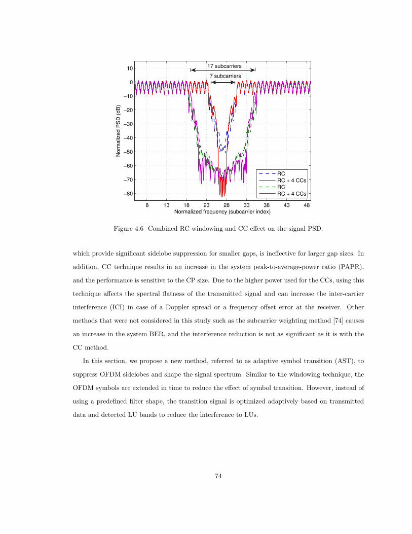
8 13 18 23 28 33 38 43 48
−80
−70
−60
−50
−40
−30
−20
−10
0
10
Normalized frequency (subcarrier index)
Norm
aliz
ed P
SD
(dB
)
RC
RC + 4 CCs
RC
RC + 4 CCs
7 subcarriers
17 subcarriers
Figure 4.6 Combined RC windowing and CC effect on the signal PSD.
which provide significant sidelobe suppression for smaller gaps, is ineffective for larger gap sizes. In
addition, CC technique results in an increase in the system peak-to-average-power ratio (PAPR),
and the performance is sensitive to the CP size. Due to the higher power used for the CCs, using this
technique affects the spectral flatness of the transmitted signal and can increase the inter-carrier
interference (ICI) in case of a Doppler spread or a frequency offset error at the receiver. Other
methods that were not considered in this study such as the subcarrier weighting method [74] causes
an increase in the system BER, and the interference reduction is not as significant as it is with the
CC method.
In this section, we propose a new method, referred to as adaptive symbol transition (AST), to
suppress OFDM sidelobes and shape the signal spectrum. Similar to the windowing technique, the
OFDM symbols are extended in time to reduce the effect of symbol transition. However, instead of
using a predefined filter shape, the transition signal is optimized adaptively based on transmitted
data and detected LU bands to reduce the interference to LUs.
74
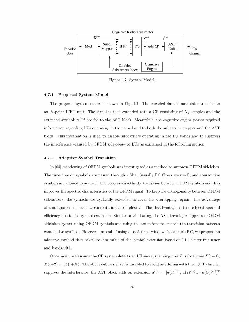
Mod.Subc.
MapperIFFT P/S Add CP
AST
UnitEncoded
data
To
channel
Cognitive Radio Transmitter
Cognitive
Engine
X(m)
x(m)
y(m)
Disabled
Subcarriers Index
Figure 4.7 System Model.
4.7.1 Proposed System Model
The proposed system model is shown in Fig. 4.7. The encoded data is modulated and fed to
an N -point IFFT unit. The signal is then extended with a CP consisting of Ng samples and the
extended symbols y(m) are fed to the AST block. Meanwhile, the cognitive engine passes required
information regarding LUs operating in the same band to both the subcarrier mapper and the AST
block. This information is used to disable subcarriers operating in the LU bands and to suppress
the interference –caused by OFDM sidelobes– to LUs as explained in the following section.
4.7.2 Adaptive Symbol Transition
In [64], windowing of OFDM symbols was investigated as a method to suppress OFDM sidelobes.
The time domain symbols are passed through a filter (usually RC filters are used), and consecutive
symbols are allowed to overlap. The process smooths the transition between OFDM symbols and thus
improves the spectral characteristics of the OFDM signal. To keep the orthogonality between OFDM
subcarriers, the symbols are cyclically extended to cover the overlapping region. The advantage
of this approach is its low computational complexity. The disadvantage is the reduced spectral
efficiency due to the symbol extension. Similar to windowing, the AST technique suppresses OFDM
sidelobes by extending OFDM symbols and using the extensions to smooth the transition between
consecutive symbols. However, instead of using a predefined window shape, such RC, we propose an
adaptive method that calculates the value of the symbol extension based on LUs center frequency
and bandwidth.
Once again, we assume the CR system detects an LU signal spanning over K subcarriers X(i+1),
X(i+2),. . .X(i+K). The above subcarrier set is disabled to avoid interfering with the LU. To further
suppress the interference, the AST block adds an extension a(m) = [a(1)(m), a(2)(m),. . . a(C)(m)]T
75
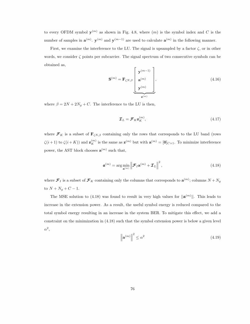
to every OFDM symbol y(m) as shown in Fig. 4.8, where (m) is the symbol index and C is the
number of samples in a(m). y(m) and y(m−1) are used to calculate a(m) in the following manner.
First, we examine the interference to the LU. The signal is upsampled by a factor ζ, or in other
words, we consider ζ points per subcarrier. The signal spectrum of two consecutive symbols can be
obtained as,
S(m) = FζN,β
y(m−1)
a(m)
y(m)
︸ ︷︷ ︸z(m)
, (4.16)
where β = 2N + 2Ng + C. The interference to the LU is then,
IL = FKz(m)K , (4.17)
where FK is a subset of FζN,β containing only the rows that corresponds to the LU band (rows
ζ(i+1) to ζ(i+K)) and z(m)K is the same as z(m) but with a(m) = [0]C×1. To minimize interference
power, the AST block chooses a(m) such that,
a(m) = arg min
a(m)
∥∥∥FIa(m) + IL
∥∥∥2
, (4.18)
where FI is a subset of FK containing only the columns that corresponds to a(m); columns N +Ng
to N + Ng + C − 1.
The MSE solution to (4.18) was found to result in very high values for ||a(m)||. This leads to
increase in the extension power. As a result, the useful symbol energy is reduced compared to the
total symbol energy resulting in an increase in the system BER. To mitigate this effect, we add a
constraint on the minimization in (4.18) such that the symbol extension power is below a given level
α2,∥∥∥a(m)
∥∥∥2
≤ α2 (4.19)
76
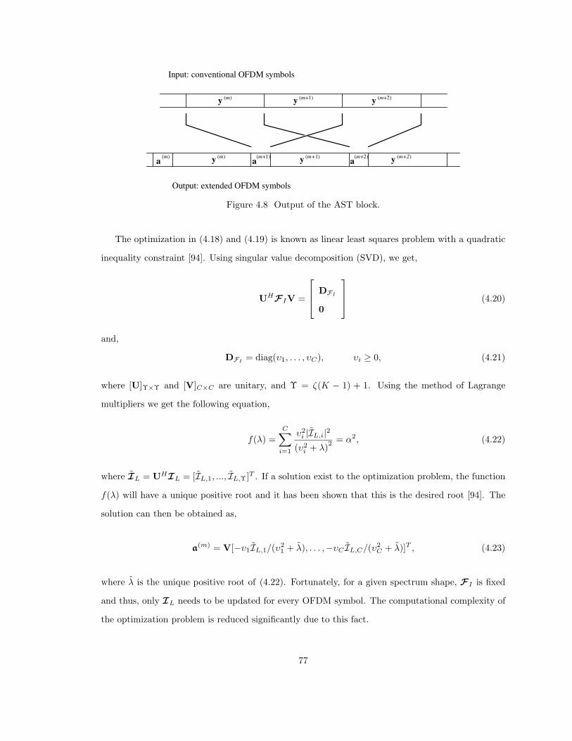
y (m) y (m+1) y (m+2)
y (m) y (m+1) y (m+2)a
Input: conventional OFDM symbols
Output: extended OFDM symbols
(m+1)a
(m)a
(m+2)
Figure 4.8 Output of the AST block.
The optimization in (4.18) and (4.19) is known as linear least squares problem with a quadratic
inequality constraint [94]. Using singular value decomposition (SVD), we get,
UHFIV =
DFI
0
(4.20)
and,
DFI= diag(υ1, . . . , υC), υi ≥ 0, (4.21)
where [U]Υ×Υ and [V]C×C are unitary, and Υ = ζ(K − 1) + 1. Using the method of Lagrange
multipliers we get the following equation,
f(λ) =C∑
i=1
υ2i |IL,i|2
(υ2i + λ)
2 = α2, (4.22)
where IL = UHIL = [IL,1, ..., IL,Υ]T . If a solution exist to the optimization problem, the function
f(λ) will have a unique positive root and it has been shown that this is the desired root [94]. The
solution can then be obtained as,
a(m) = V[−υ1IL,1/(υ2
1 + λ), . . . ,−υC IL,C/(υ2C + λ)]T , (4.23)
where λ is the unique positive root of (4.22). Fortunately, for a given spectrum shape, FI is fixed
and thus, only IL needs to be updated for every OFDM symbol. The computational complexity of
the optimization problem is reduced significantly due to this fact.
77
An important parameter for OFDM systems is the PAPR which affects the dynamic range over
which the system should be linear. By choosing α2 such that,
α2 = C/(N + Ng)ES , (4.24)
the signal average power is kept at the same level, where ES is the symbol energy prior to the AST
block. Since the AST signal is optimized to smooth the symbol transition, it does not introduce any
peaks to the signal (confirmed by simulation results) and, thus, the PAPR of the system does not
increase. Nevertheless, the AST reduces the useful symbol energy. Using (4.24), the maximum SNR
loss γ is,
γ = 10 log10
(ES + α2
ES
)= 10 log10
(1 +
C
N + Ng
)dB. (4.25)
By controlling C and for a fixed PAPR, the system has a tradeoff between reducing γ (by reducing
C), or improving the interference suppression (by increasing C).
Note that since AST technique is performed on time-domain symbols, the performance is not
sensitive to the CP size. In addition, the AST does not introduce any ISI to the system as the
leakage from the symbol extension is contained in the CP. The intended receiver can remove the
AST extension along with the CP to maintain an ISI-free signal.
4.7.3 Simulation Results
In this section, the performance of the proposed method is investigated using computer simula-
tions. We consider an OFDM-based CR system with N = 256 and Ng = 16. The AST method is
used with C = 16, ζ = 16, and, based on (4.24), α2 = 0.06ES . The DC subcarrier is disabled. Data
subcarriers are modulated with a quadrature phase shift keying (QPSK) signal. All results shown
are averaged over 10, 000 OFDM symbols. We consider two cases for performance evaluation. In
the first case, an LU is detected spaning 24 OFDM subcarriers. The system disables 32 subcarriers
leaving a guard band of 4 subcarriers on each side of the LU band. The guard bands are to allow the
signal power to decay while the AST block performs the optimization over the 24–subcarrier band.
The normalized PSD of the signal at the output of the AST block is measured and the results are
shown in Fig. 4.9. The system performance is compared with a conventional OFDM system without
any symbol extension, and with an OFDM system using RC windowing and a symbol duration equal
to the AST system. The conventional OFDM system suffers an interference level of −22 dB. The
78
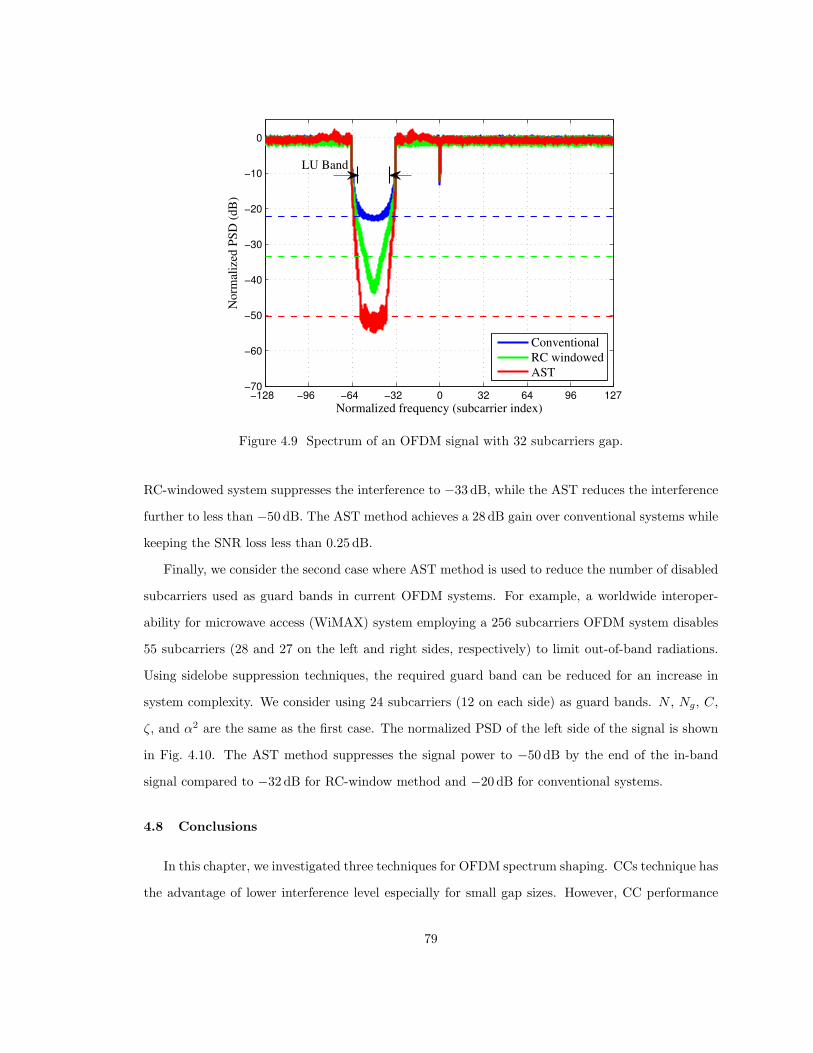
−128 −96 −64 −32 0 32 64 96 127−70
−60
−50
−40
−30
−20
−10
0
Normalized frequency (subcarrier index)
No
rmal
ized
PS
D (
dB
)
Conventional
RC windowed
AST
LU Band
Figure 4.9 Spectrum of an OFDM signal with 32 subcarriers gap.
RC-windowed system suppresses the interference to −33 dB, while the AST reduces the interference
further to less than −50 dB. The AST method achieves a 28 dB gain over conventional systems while
keeping the SNR loss less than 0.25 dB.
Finally, we consider the second case where AST method is used to reduce the number of disabled
subcarriers used as guard bands in current OFDM systems. For example, a worldwide interoper-
ability for microwave access (WiMAX) system employing a 256 subcarriers OFDM system disables
55 subcarriers (28 and 27 on the left and right sides, respectively) to limit out-of-band radiations.
Using sidelobe suppression techniques, the required guard band can be reduced for an increase in
system complexity. We consider using 24 subcarriers (12 on each side) as guard bands. N , Ng, C,
ζ, and α2 are the same as the first case. The normalized PSD of the left side of the signal is shown
in Fig. 4.10. The AST method suppresses the signal power to −50 dB by the end of the in-band
signal compared to −32 dB for RC-window method and −20 dB for conventional systems.
4.8 Conclusions
In this chapter, we investigated three techniques for OFDM spectrum shaping. CCs technique has
the advantage of lower interference level especially for small gap sizes. However, CC performance
79

−128 −124 −120 −116 −112 −108 −104 −100−70
−60
−50
−40
−30
−20
−10
0
Normalized frequency (subcarrier index)
No
rmal
ized
PS
D (
dB
)
Conventional
RC windowed
AST
Figure 4.10 Spectrum of an OFDM signal with 12 subcarriers guard band.
is sensitive to the CP size, and as the gap size increases, the performance degradation, and the
consumed power by CCs increases. Alternatively, RC windowing technique is a more robust solution
with lower complexity. The sidelobe suppression comes at the cost of an increase in the symbol
duration which reduces the spectral efficiency. However, RC windowing is inferior to CCs for small
gap sizes. The combined CCs and RC windowing technique performs very well for small gaps
regardless of the CP size. Moreover, the power consumed by CCs is minimal in this case. The
disadvantage is that the system exhibits both low spectral efficiency due to symbol extension and
higher computational complexity due to the use of CC. In addition, the combined technique does
not introduce any gain over RC windowing for large gap sizes.
Based on the above observations, we investigated a new method that can overcome the drawbacks
of RC windowing and CC technique. The proposed AST method extends OFDM symbols and uses
the extension to reduce ACI to other users operating in the same band. Simulation results show
that AST can achieve a significant gain over conventional sidelobe suppression techniques while
maintaining low increase in symbol energy. Moreover, AST does not increase the signal PAPR and
the performance is not sensitive to the CP size.
80
CHAPTER 5
ANALYSIS AND OPTIMIZATION OF OFDMA UPLINK SYSTEMS OVERTIME-VARYING FREQUENCY-SELECTIVE RAYLEIGH FADING CHANNELS
5.1 Introduction
Due to its attractive features, orthogonal frequency division multiple access (OFDMA) has
been proposed for a various wireless standards such as WiMAX [9], LTE-Advanced [14], and IST-
WINNER [15]. Most of these systems are expected to provide broadband services for mobile users.
As such, it is expected that receivers will suffer from time-varying frequency-selective propagation
effects. The quality of channel estimation, in such case, can significantly impact the overall system
performance.
To support multiple user access in OFDMA uplink (UL) systems, the OFDMA signal is divided
into smaller units, called tiles or chunks, consisting of a number of subcarriers that are adjacent in
time and frequency. One or more of these tiles can be assigned to multiple users by the scheduler
in an adaptive or random manner. Since adjacent tiles are not necessarily assigned to the same
user, it is expect that different tiles are received over different wireless channels. As such, the
channel estimation and equalization needs to be performed on a tile-by-tile basis [95, 96]. Pilots are
placed within each tile to enable the channel estimation process. The optimum allocation of pilots
within a tile to reduce the channel estimation mean-squared-error (MSE) is investigated in [97,
98] considering the frequency and time dimensions. The authors concluded that pilots should be
placed at the corners of the tile at low signal-to-noise ratio (SNR) values and at 1/√
3 of the tile
duration/bandwidth at high SNR values. In this work, pilots placement at the corners of each tile
is considered [9].
The structure of pilot assignments in OFDMA UL in the time-frequency grid is analogous to that
of pilot-symbol-aided modulation (PSAM) in single user orthogonal frequency division multiplexing
(OFDM). However, since in OFDMA UL systems, pilots in adjacent tiles cannot be used for channel
estimation, optimum algorithms such as 2D Wiener filtering [99] or higher order algorithms such
81
as sinc interpolation cannot be used [100]. In addition, techniques such as minimum mean-square
error (MMSE) channel estimation [101] are inapplicable, since the number of pilot symbols per
user/channel is not necessarily sufficient to reliably estimate the channel statistics. One approach
for channel estimation in this case is to obtain least squares (LS) estimates at pilot symbols and
use a first order time-frequency interpolation (bilinear interpolation) to estimate the channel at
data symbols. Another approach is to use iterative channel estimation methods which utilize data
symbols to improve the channel estimation process [95]. The drawback of this approach is the
increased complexity, and consequently the delay, needed to perform multiple iterations. This is
especially true for larger tile sizes, since the receiver needs to buffer the entire tile duration (up to
7560 subcarriers in some cases). In [96], the authors propose to use basis expansion model (BEM)
to describe the time-frequency selectivity of the channel within each tile, instead of a linear model.
While this method can improve the channel estimation performance, the channel Doppler spread
and delay spread values are needed to correctly model the channel. Hence, from a practical point of
view, using bilinear interpolation may be the most attractive approach for OFDMA UL systems [97].
In all the aforementioned studies, analysis of the bit error rate (BER) or optimum pilot insertion
rate for tile-based OFDMA UL system are not considered.
In this chapter, the performance of OFDMA UL system over time-varying frequency-selective
Rayleigh fading channels is considered. It is assumed that the system uses a tile-based channel
estimation and equalization approach. Considering time-frequency interpolation filter, the variances
of the channel estimates and channel estimation errors are evaluated. Expressions for the BER
performance under channel estimation errors for quadrature phase shift keying (QPSK) and quadra-
ture amplitude modulation (QAM) signals are derived. Based on the presented results, an analysis
of optimum tile dimensions (or equivalently pilot insertion rate) that maximize the overall system
throughput is investigated.
The remainder of this chapter is organized as follows. In Section 5.2, the system model and
considered channel model are introduced. Evaluation of the channel estimation and equalization
using time-frequency interpolation is presented in Section 5.3. Analysis of the BER performance
for QPSK and QAM signals is derived in Section 5.4. In Section 5.5, optimum tile dimensions for
maximum system throughput is discussed. Simulation results are used to verify the theoretically
results in Section 5.6. Finally, concluding remarks are presented in Section 5.7.
82
5.2 System Model
5.2.1 Channel Model
The complex baseband representation of a mobile wireless channel impulse response (CIR) is
described as [101],
h(t, τ) =∑
`
h`(t)δ(t − τ`), (5.1)
where τ` is the delay of the lth path and h`(t) is the corresponding complex amplitude. Note that
h`(t)’s are wide-sense stationary (WSS) narrowband complex Gaussian processes, and are indepen-
dent for different paths. Without the loss of generality, the channel is assumed to be normalized
such that
∑
`
σ2` = 1 (5.2)
where
σ2` = E
{|h`(t)|2
}(5.3)
and E{·} is the expectation operator. The channel frequency response (CFR) at time t is,
H(t, f) =∑
`
h`(t) exp (−2πfτ`) . (5.4)
The channel fading in time is modeled using the classical Doppler spectrum [102]. Thus, for an
OFDM system with symbol duration TS and subcarrier spacing ∆f , the correlation function between
the channel responses at two subcarriers (n, k) and (n + ∆n, k + ∆k) is [101],
RH(∆n,∆k) = J0(2π∆nfd)∑
`
σ2` exp (−2π∆k∆fτ`) (5.5)
where J0 is the zeroth-order Bessel function of the first kind, fd is the maximum Doppler shift, and
n and k are the symbol index and subcarrier index, respectively, such that
RH(∆n,∆k) ≡ RH(∆nTS ,∆k∆f). (5.6)
83
5.2.2 Signal Model
In OFDMA systems, used subcarriers are divided into smaller blocks, also known as tiles or
chunks, which represent the minimum allocation unit. The tiles are then assigned to subchannels
either randomly or depending on user channels. The overall received UL frame is a sum of all current
user signals, which are transmitted over different communication channels.
An example of how the UL frame is divided into tiles is shown in Fig. 5.1. Used subcarriers are
divided into Q tiles, usually with equal number of tiles on each side of the DC subcarrier. Three
different tile structures are shown in the figure, where tile dimensions are three symbols by four
subcarriers. In this example, the tile bandwidth, Btile = 3∆f , and the tile duration, Ttile = 2TS .
For the remainder of this chapter, Tile C structure is considered. Note that a similar frame structure
is employed by the mobile worldwide interoperability for microwave access (WiMAX) standard [9].
An OFDMA-UL system employing N subcarriers per symbol is considered. The DC subcarrier
and guard subcarriers are disabled. The remaining subcarriers Nu are used for data transmission
with equal number of subcarriers on each side of the DC subcarrier. The above assumptions are
common for most practical implementations of OFDMA systems.
Considering the output of the fast Fourier transform (FFT) unit at the receiver, the received
signal of a user u at subcarrier (n, k) is
Y (n, k) = H(u)(n, k)X(u)(n, k) + I(n, k) + W (n, k), (5.7)
where X(u)(n, k) and H(u)(n, k) are the uth user transmitted signal and CFR at subcarrier (n, k),
respectively, W (n, k) is the additive white Gaussian noise (AWGN) with zero mean and variance
σ2n = N0/2, and I(n, k) is the inter-carrier interference (ICI) due to Doppler spreading. It is shown
in [103] that,
I(n, k) =1
N
N∑
i=0,i 6=k
X(n, i)N−1∑
m=0
H(n, i,m) exp(2πm(i − k)/N) (5.8)
where H(n, i,m) is the CFR at subcarrier (n, i) and sampling instant m, as the channel is assumed
to be time variant. Whenever the sampling index is dropped, it is to indicate averaging is performed
84
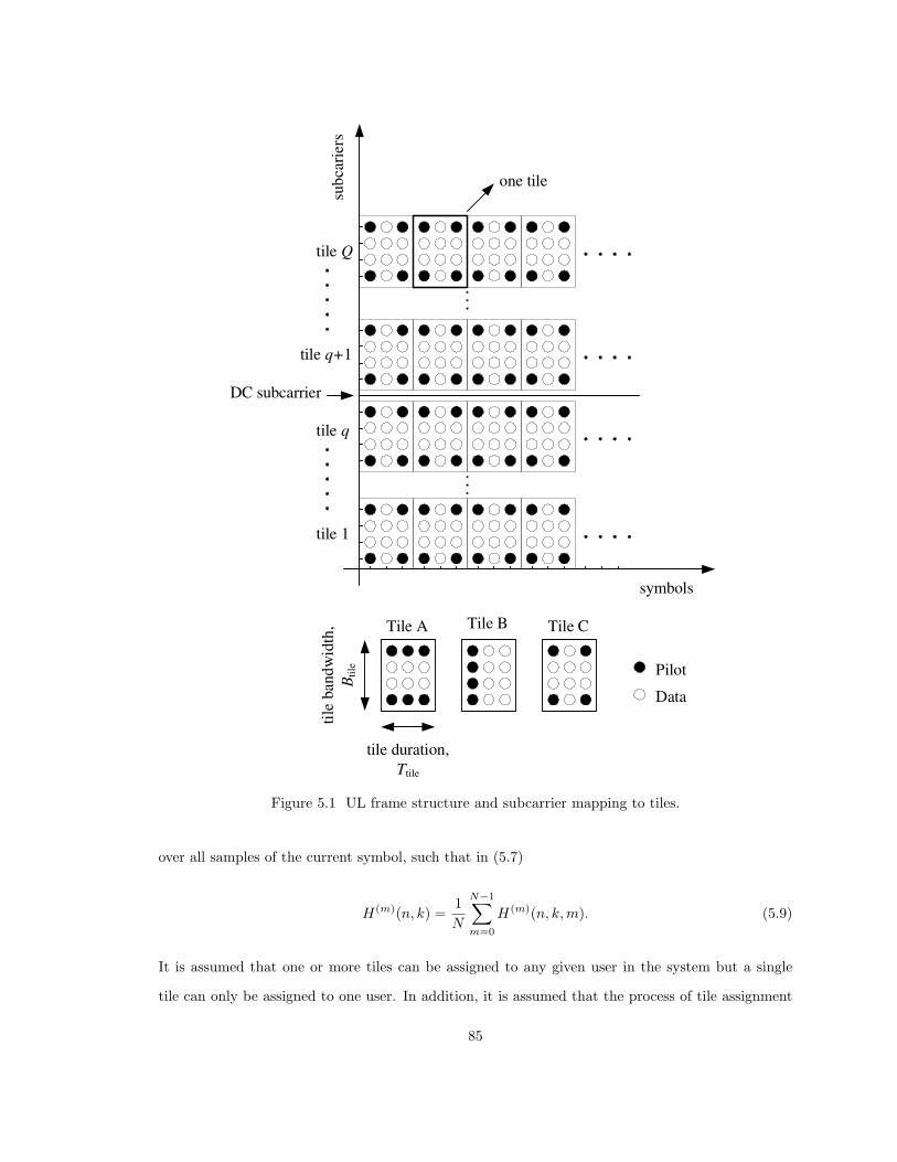
symbols
sub
cari
ers
Pilot
Data
Tile A Tile B Tile C
one tile
tile duration,
Ttile
tile
ban
dw
idth
,
Bti
le
DC subcarrier
tile q
tile 1
tile Q
tile q+1
Figure 5.1 UL frame structure and subcarrier mapping to tiles.
over all samples of the current symbol, such that in (5.7)
H(m)(n, k) =1
N
N−1∑
m=0
H(m)(n, k,m). (5.9)
It is assumed that one or more tiles can be assigned to any given user in the system but a single
tile can only be assigned to one user. In addition, it is assumed that the process of tile assignment
85
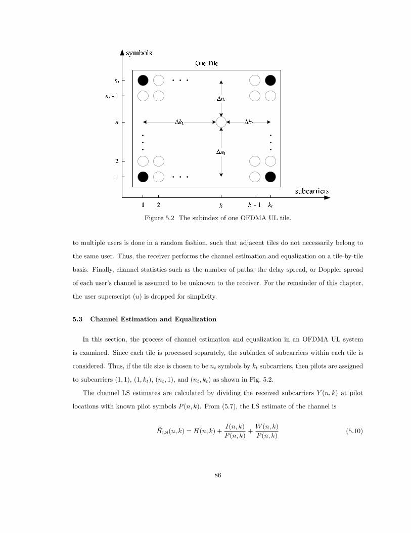
}~����}
}���������}� � �� � � ����
��� ������ � ���
�� ���
������ ���
Figure 5.2 The subindex of one OFDMA UL tile.
to multiple users is done in a random fashion, such that adjacent tiles do not necessarily belong to
the same user. Thus, the receiver performs the channel estimation and equalization on a tile-by-tile
basis. Finally, channel statistics such as the number of paths, the delay spread, or Doppler spread
of each user’s channel is assumed to be unknown to the receiver. For the remainder of this chapter,
the user superscript (u) is dropped for simplicity.
5.3 Channel Estimation and Equalization
In this section, the process of channel estimation and equalization in an OFDMA UL system
is examined. Since each tile is processed separately, the subindex of subcarriers within each tile is
considered. Thus, if the tile size is chosen to be nt symbols by kt subcarriers, then pilots are assigned
to subcarriers (1, 1), (1, kt), (nt, 1), and (nt, kt) as shown in Fig. 5.2.
The channel LS estimates are calculated by dividing the received subcarriers Y (n, k) at pilot
locations with known pilot symbols P (n, k). From (5.7), the LS estimate of the channel is
HLS(n, k) = H(n, k) +I(n, k)
P (n, k)+
W (n, k)
P (n, k)(5.10)
86
where n ∈ {1, nt} and k ∈ {1, kt}, for each tile. Without the loss of generality, it is assumed that
data symbols and pilot symbols are normalized such that E{|X(n, k)|2} = E{|P (n, k)|2} = 1. Thus,
the second order statistics of I(n, k) and W (n, k) are not changed when divided by P (n, k). The ICI
can be modeled as an additive Gaussian process with zero mean and variance σ2ICI [104]. An upper
bound on σ2ICI for the classical Doppler spectrum is introduced in [105] as
σ2ICI ≤
1
24(2πfdTs)
2. (5.11)
Assuming the ICI and AWGN values at each subcarrier are independent and identically distributed
(i.i.d.), the correlation function between the LS estimates at two subcarriers (n, k) and (n+∆n, k +
∆k) can be shown, using (5.10) and (5.6), to be
RH,LS(∆n,∆k) =
σ2H + σ2
ICI + σ2n, for ∆n = ∆k = 0,
RH(∆n,∆k), otherwise
(5.12)
where
σ2H = E
[|H(n, k)|2
]. (5.13)
Since the channel is assumed to be normalized, then from (5.2), we conclude that σ2H = 1.
The receiver estimates the channel at data subcarriers using bilinear interpolation and the four
LS estimates. For a data subcarrier (n, k) that belongs to the current tile, the bilinear channel
estimate is calculated as follows
HBL(n, k) =1
∆nT ∆kT
[∆nt ∆n1
]
HLS(1, 1) HLS(1, kt)
HLS(nt, 1) HLS(nt, kt)
∆kt
∆k1
(5.14)
where
∆n1 = n − 1, ∆nt = nt − n, ∆nT = nt − 1,
∆k1 = k − 1, ∆kt = kt − k, ∆kT = kt − 1, (5.15)
87
as shown in Fig. 5.2. Using zero-forcing (ZF) equalizer, the equalized OFDMA subcarrier is given
by
X(n, k) =Y (n, k)
HBL(n, k)
=X(n, k) − ε(n, k)
HBL(n, k)X(n, k) +
I(n, k)
HBL(n, k)+
W (n, k)
HBL(n, k)(5.16)
where
ε(n, k) = HBL(n, k) − H(n, k) (5.17)
is the channel estimation error at data subcarrier (n, k).
5.4 Bit Error Rate Analysis
In this section, the BER of OFDMA UL systems operating in multipath slow fading channels
is evaluated. The BER of systems, including OFDM systems, under channel estimation errors has
been studied in the literature [100, 106–112]. Evaluation of BER, assuming the channel envelop and
phase are two independent random processes, is introduced in [106] without considering ICI and
in [107, 110] while taking ICI into consideration. In [110, 111], the BER is evaluated while taking
into account the correlation between the envelop and the phase of the channel. In [100], the results
are extended to Ricean fading channels and multichannel receivers. However, the calculation of BER
in most of the above references involves the evaluation of three-fold (or even four-fold) integral and
yields highly-complex expressions. An approximation of the BER for OFDM-based wireless local
area network (WLAN) systems with channel estimation errors is introduced in [108]. The authors
assumed that for relatively small channel estimation errors, the estimated channel response and the
channel estimation errors are uncorrelated. In this work, we use the results introduced in [108], since
they yield simplified expressions with minimal error margin for considered application (as verified
by computer simulations in Section 5.6).
From (5.16), it can be seen that the sources of degradation are the bilinear channel estimates,
the channel estimation error, the ICI, and the AWGN, with powers (or variances) σ2BL, σ2
ε , σ2ICI,
and σ2n, respectively. Note that the symbol power is not considered here, since it is assumed that
symbols are normalized. To evaluate the BER, the instantaneous SNR is obtained at any subcarrier
88

(n, k) using (5.16) such that
SNR(n, k) =
∣∣∣HBL(n, k)∣∣∣2
|ε(n, k)|2 + σ2ICI + σ2
n
. (5.18)
The instantaneous BER is evaluated for a given modulation type using (5.18), and the average BER
is obtained by averaging over the probability density functions (PDF) of both the channel estimation
error and the channel estimates. The BER for a QPSK signal is [108]
PQPSK ≈ 1
2
[1 −
√πσ2
BL
2σ2ε
exp(ξ) erfc(√
ξ)]
(5.19)
where erfc(·) is the complementary error function and
ξ =σ2
BL + 2σ2ICI + 2σ2
n
2σ2ε
. (5.20)
For square QAM signals, i.e. with even number of bits per symbol, and with Gray bit mapping, the
BER is [108]
PQAM ≈ 2
log2 M
(1 − 1√
M
)[1 −
√3πσ2
BL
2(M − 1)σ2ε
exp(ξM ) erfc(√
ξM
)](5.21)
where M is the modulation order and
ξM =3σ2
BL + 2(M − 1)(σ2ICI + σ2
n)
2(M − 1)σ2ε
. (5.22)
For low channel estimation errors, ξ and ξM yield large values, as can be seen from (5.20) and (5.22).
However, evaluating the erfc(·) of large values can lead to inaccurate results. To overcome this
problem, we further simplify the expressions in (5.19) and (5.21) by using an approximation of the
erfc(·). It can be shown from [113] that the erfc(·) is bounded by
L0(x) < erfc(x) ≤ R0(x) (5.23)
89
where
L0(x) =2 exp(−x2)
√π(x +
√x2 + 2
) (5.24)
and
R0(x) =2 exp(−x2)
√π(x +
√x2 + 4/π
) . (5.25)
For large vaules of x, such as in considered application, we note that
erfc(x) ≈ L0(x). (5.26)
Applying (5.26) to (5.19) and (5.21), the BER for QPSK signals reduces to
PQPSK ≈ 1
2
[1 −
√2σ2
BL
σ2ε
1√ξ +
√ξ + 2
](5.27)
and for QAM signals reduces to
PQAM ≈ 2
log2 M
(1 − 1√
M
)[1 −
√6σ2
BL
(M − 1)σ2ε
· 1√ξM +
√ξM + 2
]. (5.28)
The above two expressions for the BER have the advantages of being much simpler compared with
exact BER expressions in the literature, can be evaluated accurately for low channel estimation
errors (no erfc(·)), and provide very close results to the exact BER as shown in Section 5.6.
To use the BER expressions presented in (5.27) and (5.28), the power of the channel estimates
σ2BL and channel estimation errors σ2
ε need to be calculated. The value of σ2BL is expressed as
σ2BL =
1
ntkt − 4
∑
n
∑
k
σ2BL(n, k) (5.29)
and
σ2BL(n, k) = E
{∣∣∣HBL(n, k)∣∣∣2}
(5.30)
90

where the summations are over all data subcarriers within the tile and σ2BL(n, k) is the variance of
the channel estimates at subcarrier (n, k). From (5.10) and (5.14), and since I(n, k) and W (n, k)
are i.i.d. zero mean random variables, it can be shown that
σ2BL(n, k) =
1
∆n2T ∆k2
T
[(∆n2
t ∆k2t + ∆n2
1∆k2t + ∆n2
t ∆k21 + ∆n2
1∆k21)<{RH,LS(0, 0)}
+ 2∆n1∆nt(∆k21 + ∆k2
t )<{RH,LS(∆nT , 0)} + 2∆k1∆kt(∆n21 + ∆n2
t )<{RH,LS(0,∆kT )}
+ ∆n1∆nt∆k1∆kt<{RH,LS(∆nT ,∆kT )}]
(5.31)
where <{x} is the real part of x. The above relation can be expressed in matrix form as follows
σ2BL(n, k) =
1
∆n2T ∆k2
T
n<{RA}k (5.32)
where
n =
[∆n2
1 + ∆n2t 2∆n1∆nt
], (5.33)
RA =
RH,LS(0, 0) RH,LS(0,∆kT )
RH,LS(∆nT , 0) RH,LS(∆nT ,∆kT )
, (5.34)
and
k =
∆k21 + ∆k2
t
2∆k1∆kt
. (5.35)
Note that RA is independent of the subcarrier index (n, k). The value of RA can be related to
channel correlation function RH(∆n,∆k) using (5.12) such that
RA =
σ2H + σ2
ICI + σ2n RH(0,∆kT )
RH(∆nT , 0) RH(∆nT ,∆kT )
. (5.36)
91
Similar to σ2LS, the variance of the channel estimation error can be calculated from (5.17) as
follows
σ2ε =
1
ntkt − 4
∑
n
∑
k
σ2ε (n, k) (5.37)
and
σ2ε (n, k) = σ2
H + σ2BL − 2<
{E[H∗(n, k)HBL(n, k)
]
︸ ︷︷ ︸RB(n,k)
}. (5.38)
From (5.14), it can be shown that
RB(n, k) =1
∆nT ∆kT
[∆nt ∆n1
]
RH(∆n1,∆k1) RH(∆n1,∆kt)
RH(∆nt,∆k1) RH(∆nt,∆kt)
∆kt
∆k1
. (5.39)
Based on the results in (5.29), (5.32), (5.36), (5.37), (5.38), and (5.39); the values of σ2BL and σ2
ε can
be calculated using the channel autocorrelation function and the considered tile dimensions (nt and
kt).
5.5 Optimum Tile Dimensions
Next, optimization of the tile dimensions, using the results presented is this chapter, is consid-
ered. For the system under consideration, it is assumed that hard decision detection and decoding
is used at the receiver. Similar analysis can be applied to the soft decision detection case. How-
ever, calculations of soft decision metrics over Rayleigh channels with channel estimation errors is
quite complicated [114, 115] and is out of the scope of this work. Two approaches are considered
under hard decision criteria. The first approach is to choose the tile dimension that maximizes
the system throughput, assuming optimum channel coding. The second approach is to consider
the tile dimensions that maximize the system effective throughput under practical channel coding
conditions.
With sufficient interleaving, the channel can be modeled as a binary symmetric channel (BSC)
with BER Pb which can be obtained using (5.27) and (5.28). In this case, the channel capacity
92
is [89, p. 382]
C = Pb log2(2Pb) + (1 − Pb) log2 2(1 − Pb). (5.40)
From the noisy channel coding theorem [116], the maximum coding rate that can achieve error-
free transmission is equal to C. Thus, for given tile dimensions (nt, kt), the maximum achievable
throughput is
Tmax = C log2 Mntkt − 4
ntkt
Nu
TS. (5.41)
It can be seen from (5.41) that increasing the tile dimensions, which effectively reduces the pilot
insertion rate, can increase the system throughput. However, larger tile dimensions degrade the
channel estimation performance leading to high BER, Pb and consequently lower channel capacity,
C. As such, there is an optimum value for nt and kt at which the throughput is maximized.
The optimum tile dimensions in that sense can be obtained using numerical methods as shown in
Section 5.6.
Achieving the channel capacity using channel coding is usually very difficult in practice. Thus,
using the above approach may result in tile dimensions that are not optimum for a practical system.
In this case, the system design may consider choosing the tile dimensions that maximize the system
effective throughput, where the effective throughput is defined as
Teff = rc(1 − Pf ) log2 Mntkt − 4
ntkt
Nu
TS, (5.42)
where rc is the channel coding rate, which is usually predefined in a practical system, and Pf is the
frame error rate (FER). The above expression is based on the fact that for practical systems, the
decoded frames are checked for errors and erroneous frames are dropped. Thus, the actual system
throughput is based on the rate of frames that are received successfully. Similar to the previous
approach, while increasing the tile dimensions can increase the system throughput, it leads to higher
FER which may cancel any increase to the overall system throughput. Therefore, it is expected that
there should be optimum tile dimensions, that maximize the effective throughput.
93
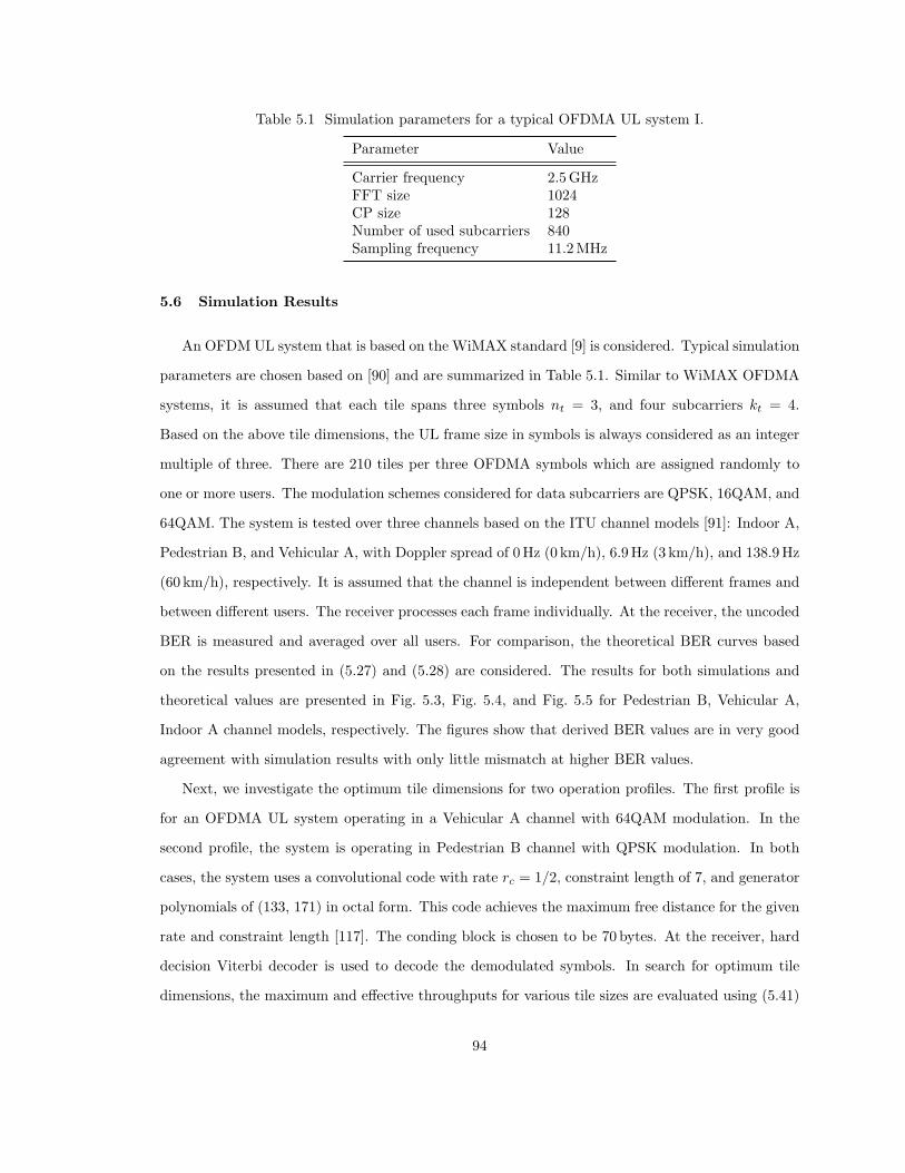
Table 5.1 Simulation parameters for a typical OFDMA UL system I.
Parameter Value
Carrier frequency 2.5 GHzFFT size 1024CP size 128Number of used subcarriers 840Sampling frequency 11.2 MHz
5.6 Simulation Results
An OFDM UL system that is based on the WiMAX standard [9] is considered. Typical simulation
parameters are chosen based on [90] and are summarized in Table 5.1. Similar to WiMAX OFDMA
systems, it is assumed that each tile spans three symbols nt = 3, and four subcarriers kt = 4.
Based on the above tile dimensions, the UL frame size in symbols is always considered as an integer
multiple of three. There are 210 tiles per three OFDMA symbols which are assigned randomly to
one or more users. The modulation schemes considered for data subcarriers are QPSK, 16QAM, and
64QAM. The system is tested over three channels based on the ITU channel models [91]: Indoor A,
Pedestrian B, and Vehicular A, with Doppler spread of 0 Hz (0 km/h), 6.9 Hz (3 km/h), and 138.9 Hz
(60 km/h), respectively. It is assumed that the channel is independent between different frames and
between different users. The receiver processes each frame individually. At the receiver, the uncoded
BER is measured and averaged over all users. For comparison, the theoretical BER curves based
on the results presented in (5.27) and (5.28) are considered. The results for both simulations and
theoretical values are presented in Fig. 5.3, Fig. 5.4, and Fig. 5.5 for Pedestrian B, Vehicular A,
Indoor A channel models, respectively. The figures show that derived BER values are in very good
agreement with simulation results with only little mismatch at higher BER values.
Next, we investigate the optimum tile dimensions for two operation profiles. The first profile is
for an OFDMA UL system operating in a Vehicular A channel with 64QAM modulation. In the
second profile, the system is operating in Pedestrian B channel with QPSK modulation. In both
cases, the system uses a convolutional code with rate rc = 1/2, constraint length of 7, and generator
polynomials of (133, 171) in octal form. This code achieves the maximum free distance for the given
rate and constraint length [117]. The conding block is chosen to be 70 bytes. At the receiver, hard
decision Viterbi decoder is used to decode the demodulated symbols. In search for optimum tile
dimensions, the maximum and effective throughputs for various tile sizes are evaluated using (5.41)
94
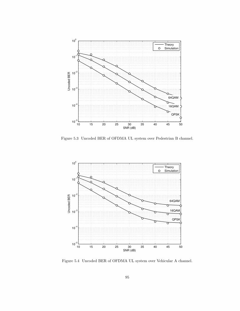
10 15 20 25 30 35 40 45 5010
−5
10−4
10−3
10−2
10−1
100
SNR (dB)
Un
co
de
d B
ER
Theory
Simulation
QPSK
64QAM
16QAM
Figure 5.3 Uncoded BER of OFDMA UL system over Pedestrian B channel.
10 15 20 25 30 35 40 45 5010
−5
10−4
10−3
10−2
10−1
100
SNR (dB)
Un
co
de
d B
ER
Theory
Simulation
64QAM
16QAM
QPSK
Figure 5.4 Uncoded BER of OFDMA UL system over Vehicular A channel.
95
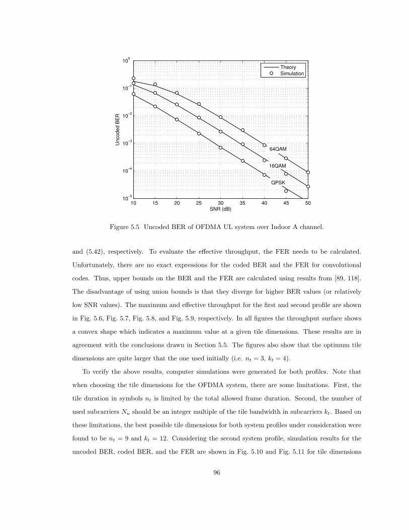
10 15 20 25 30 35 40 45 5010
−5
10−4
10−3
10−2
10−1
100
SNR (dB)
Un
co
de
d B
ER
Theory
Simulation
QPSK
16QAM
64QAM
Figure 5.5 Uncoded BER of OFDMA UL system over Indoor A channel.
and (5.42), respectively. To evaluate the effective throughput, the FER needs to be calculated.
Unfortunately, there are no exact expressions for the coded BER and the FER for convolutional
codes. Thus, upper bounds on the BER and the FER are calculated using results from [89, 118].
The disadvantage of using union bounds is that they diverge for higher BER values (or relatively
low SNR values). The maximum and effective throughput for the first and second profile are shown
in Fig. 5.6, Fig. 5.7, Fig. 5.8, and Fig. 5.9, respectively. In all figures the throughput surface shows
a convex shape which indicates a maximum value at a given tile dimensions. These results are in
agreement with the conclusions drawn in Section 5.5. The figures also show that the optimum tile
dimensions are quite larger that the one used initially (i.e. nt = 3, kt = 4).
To verify the above results, computer simulations were generated for both profiles. Note that
when choosing the tile dimensions for the OFDMA system, there are some limitations. First, the
tile duration in symbols nt is limited by the total allowed frame duration. Second, the number of
used subcarriers Nu should be an integer multiple of the tile bandwidth in subcarriers kt. Based on
these limitations, the best possible tile dimensions for both system profiles under consideration were
found to be nt = 9 and kt = 12. Considering the second system profile, simulation results for the
uncoded BER, coded BER, and the FER are shown in Fig. 5.10 and Fig. 5.11 for tile dimensions
96
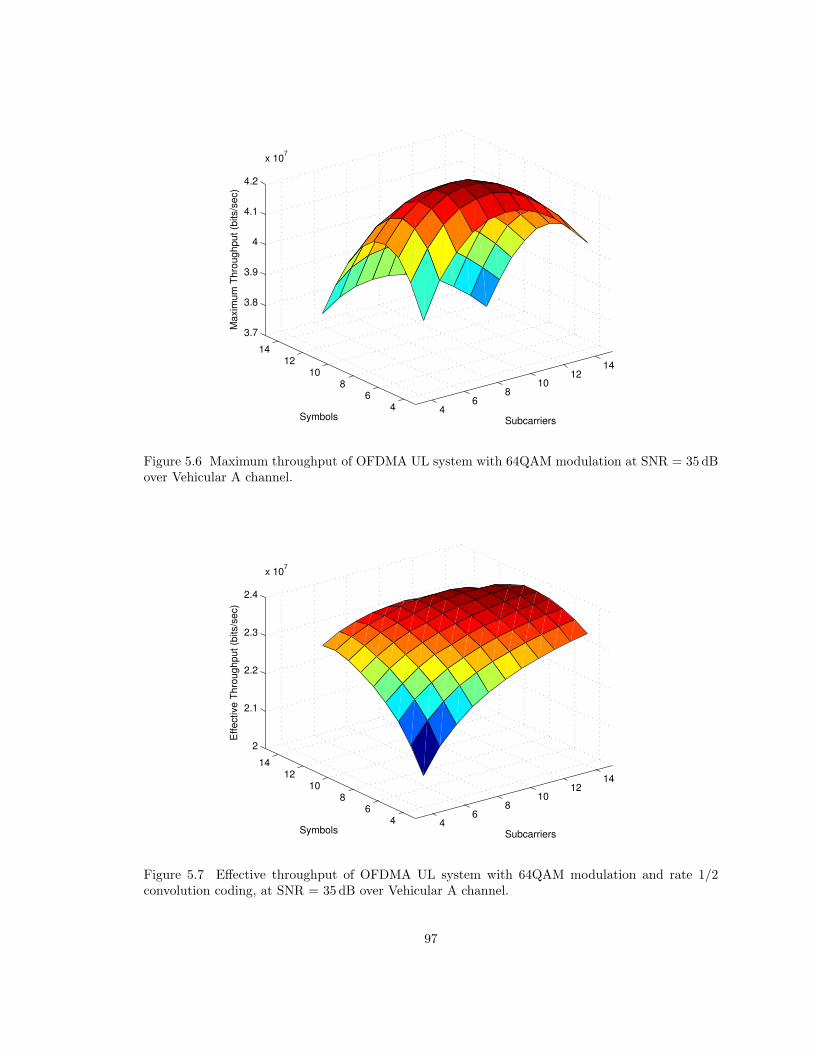
46
810
1214
46
810
1214
3.7
3.8
3.9
4
4.1
4.2
x 107
SubcarriersSymbols
Ma
xim
um
Th
rou
gh
pu
t (b
its/s
ec)
Figure 5.6 Maximum throughput of OFDMA UL system with 64QAM modulation at SNR = 35 dBover Vehicular A channel.
46
810
1214
46
810
1214
2
2.1
2.2
2.3
2.4
x 107
SubcarriersSymbols
Eff
ective
Th
rou
gh
pu
t (b
its/s
ec)
Figure 5.7 Effective throughput of OFDMA UL system with 64QAM modulation and rate 1/2convolution coding, at SNR = 35 dB over Vehicular A channel.
97
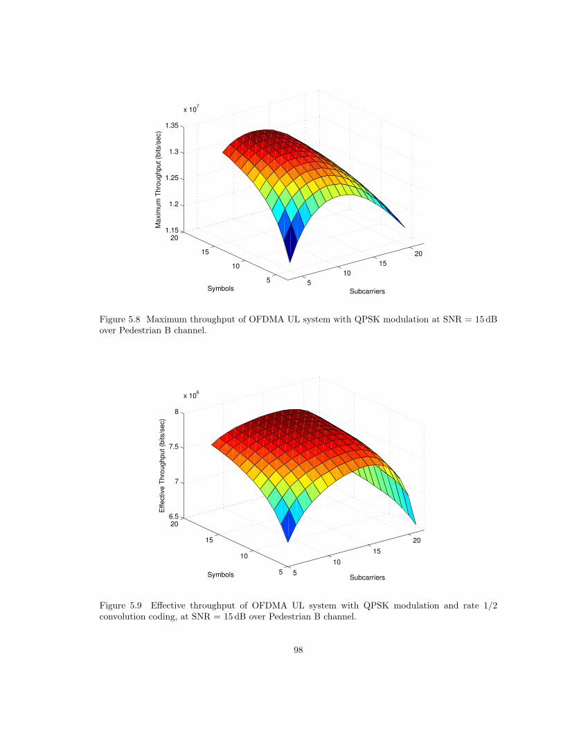
5
10
15
20
5
10
15
201.15
1.2
1.25
1.3
1.35
x 107
SubcarriersSymbols
Ma
xim
um
Th
rou
gh
pu
t (b
its/s
ec)
Figure 5.8 Maximum throughput of OFDMA UL system with QPSK modulation at SNR = 15 dBover Pedestrian B channel.
5
10
15
20
5
10
15
206.5
7
7.5
8
x 106
SubcarriersSymbols
Eff
ective
Th
rou
gh
pu
t (b
its/s
ec)
Figure 5.9 Effective throughput of OFDMA UL system with QPSK modulation and rate 1/2convolution coding, at SNR = 15 dB over Pedestrian B channel.
98
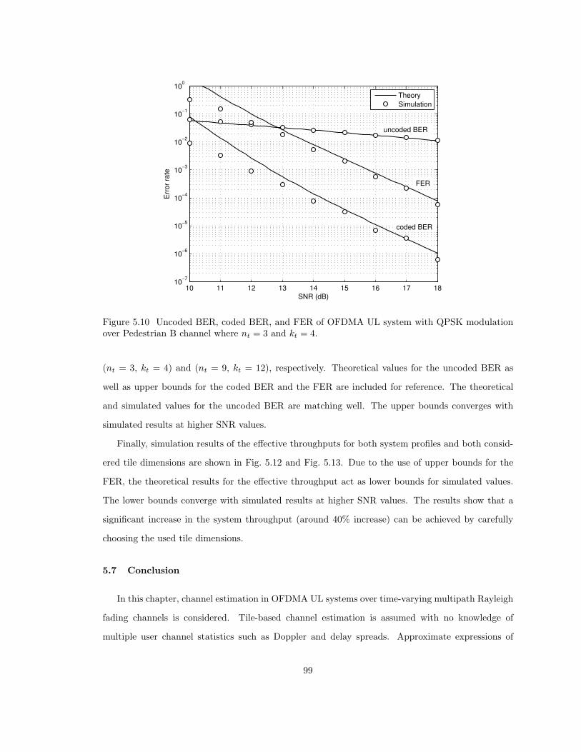
10 11 12 13 14 15 16 17 1810
−7
10−6
10−5
10−4
10−3
10−2
10−1
100
SNR (dB)
Err
or
rate
Theory
Simulation
uncoded BER
FER
coded BER
Figure 5.10 Uncoded BER, coded BER, and FER of OFDMA UL system with QPSK modulationover Pedestrian B channel where nt = 3 and kt = 4.
(nt = 3, kt = 4) and (nt = 9, kt = 12), respectively. Theoretical values for the uncoded BER as
well as upper bounds for the coded BER and the FER are included for reference. The theoretical
and simulated values for the uncoded BER are matching well. The upper bounds converges with
simulated results at higher SNR values.
Finally, simulation results of the effective throughputs for both system profiles and both consid-
ered tile dimensions are shown in Fig. 5.12 and Fig. 5.13. Due to the use of upper bounds for the
FER, the theoretical results for the effective throughput act as lower bounds for simulated values.
The lower bounds converge with simulated results at higher SNR values. The results show that a
significant increase in the system throughput (around 40% increase) can be achieved by carefully
choosing the used tile dimensions.
5.7 Conclusion
In this chapter, channel estimation in OFDMA UL systems over time-varying multipath Rayleigh
fading channels is considered. Tile-based channel estimation is assumed with no knowledge of
multiple user channel statistics such as Doppler and delay spreads. Approximate expressions of
99
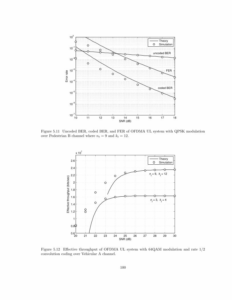
10 11 12 13 14 15 16 17 1810
−7
10−6
10−5
10−4
10−3
10−2
10−1
100
SNR (dB)
Err
or
rate
Theory
Simulation
uncoded BER
coded BER
FER
Figure 5.11 Uncoded BER, coded BER, and FER of OFDMA UL system with QPSK modulationover Pedestrian B channel where nt = 9 and kt = 12.
20 21 22 23 24 25 26 27 28 29 300.6
0.8
1
1.2
1.4
1.6
1.8
2
2.2
2.4
2.6
x 107
SNR (dB)
Eff
ective
th
rou
gh
pu
t (b
its/s
ec)
Theory
Simulation
nt = 9, k
t = 12
nt = 3, k
t = 4
Figure 5.12 Effective throughput of OFDMA UL system with 64QAM modulation and rate 1/2convolution coding over Vehicular A channel.
100
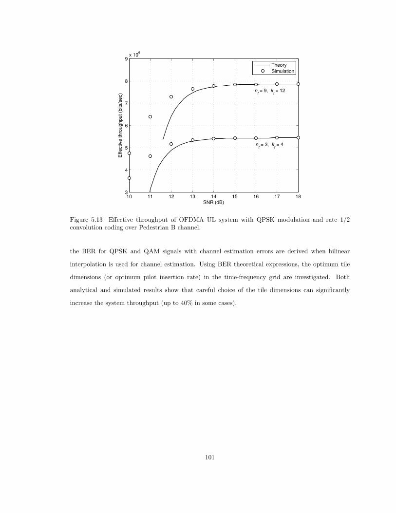
10 11 12 13 14 15 16 17 183
4
5
6
7
8
9x 10
6
SNR (dB)
Eff
ective
th
rou
gh
pu
t (b
its/s
ec)
Theory
Simulation
nt = 9, k
t = 12
nt = 3, k
t = 4
Figure 5.13 Effective throughput of OFDMA UL system with QPSK modulation and rate 1/2convolution coding over Pedestrian B channel.
the BER for QPSK and QAM signals with channel estimation errors are derived when bilinear
interpolation is used for channel estimation. Using BER theoretical expressions, the optimum tile
dimensions (or optimum pilot insertion rate) in the time-frequency grid are investigated. Both
analytical and simulated results show that careful choice of the tile dimensions can significantly
increase the system throughput (up to 40% in some cases).
101
CHAPTER 6
IQ IMBALANCE CORRECTION FOR OFDMA UPLINK SYSTEMS
6.1 Introduction
The direct conversion receiver is an attractive architecture for the physical layer (PHY) of or-
thogonal frequency division multiple access (OFDMA) systems since it avoids costly intermediate
frequency (IF) filters, reduces power consumption, and allows for easier integration than super-
heterodyne structure [17]. However, direct conversion receivers cause more distortions to the base-
band signal due to the imbalance between the inphase (I) and quadrature (Q) branches. The IQ
imbalance results in a degradation in the system performance. This drawback of direct conversion
receivers becomes more significant with orthogonal frequency division multiplexing (OFDM) systems
as they are known to be sensitive to receiver front-end non-idealities [18]. Thus, there is a need for
methods to nullify or reduce the IQ distortions.
Several techniques have been proposed to reduce the degradation caused by IQ imbalance in
OFDM-based systems [119]. In [120–122], the IQ imbalance caused by the receiver front-end is
investigated. The combined effects of IQ imbalance at the transmitter and receiver front-ends is
investigated in [123–126]. An interesting approach that uses the influence of IQ imbalance to obtain
diversity gain is proposed in [127].
In all of the above, the effects of IQ imbalance on multiuser OFDM systems are not considered.
In OFDMA-uplink (UL) systems, IQ imbalance problem becomes more complicated. First, the non-
idealities in multiple user front-ends are expected to be different. Second, the total IQ imbalance
effects on OFDMA systems results in multiuser interference (MUI) as opposed to inter-carrier inter-
ference (ICI) in OFDM systems. In addition, in OFDMA-UL systems, preambles are not used for
channel estimation. Instead, the channel is divided into subchannels -that can be assigned to users-
with dedicated pilots for each subchannel. Without preambles, many of proposed algorithms above
are inapplicable.
102
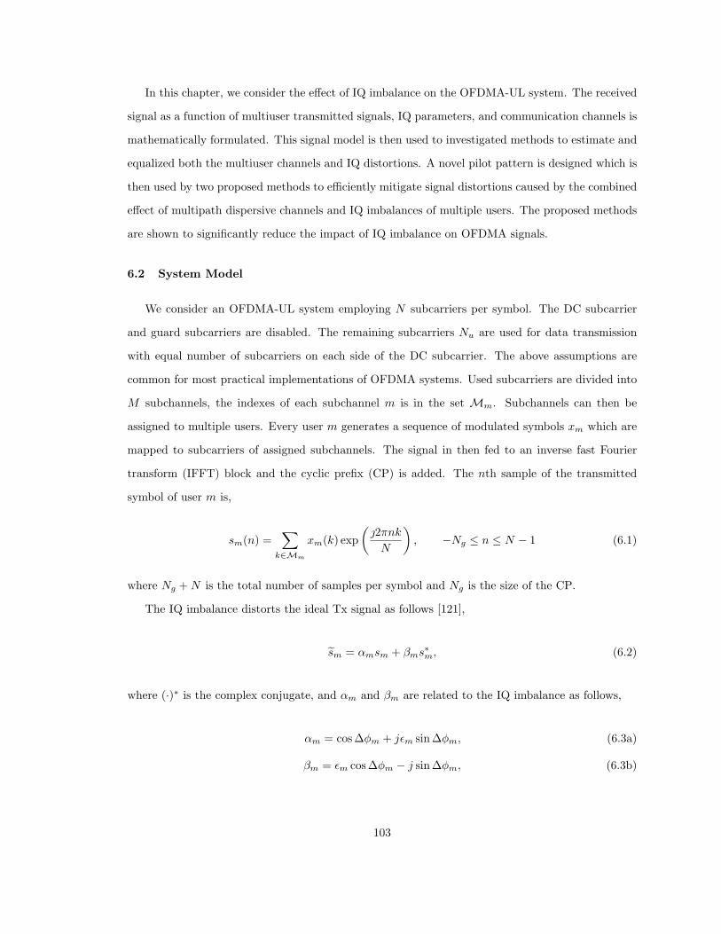
In this chapter, we consider the effect of IQ imbalance on the OFDMA-UL system. The received
signal as a function of multiuser transmitted signals, IQ parameters, and communication channels is
mathematically formulated. This signal model is then used to investigated methods to estimate and
equalized both the multiuser channels and IQ distortions. A novel pilot pattern is designed which is
then used by two proposed methods to efficiently mitigate signal distortions caused by the combined
effect of multipath dispersive channels and IQ imbalances of multiple users. The proposed methods
are shown to significantly reduce the impact of IQ imbalance on OFDMA signals.
6.2 System Model
We consider an OFDMA-UL system employing N subcarriers per symbol. The DC subcarrier
and guard subcarriers are disabled. The remaining subcarriers Nu are used for data transmission
with equal number of subcarriers on each side of the DC subcarrier. The above assumptions are
common for most practical implementations of OFDMA systems. Used subcarriers are divided into
M subchannels, the indexes of each subchannel m is in the set Mm. Subchannels can then be
assigned to multiple users. Every user m generates a sequence of modulated symbols xm which are
mapped to subcarriers of assigned subchannels. The signal in then fed to an inverse fast Fourier
transform (IFFT) block and the cyclic prefix (CP) is added. The nth sample of the transmitted
symbol of user m is,
sm(n) =∑
k∈Mm
xm(k) exp
(2πnk
N
), −Ng ≤ n ≤ N − 1 (6.1)
where Ng + N is the total number of samples per symbol and Ng is the size of the CP.
The IQ imbalance distorts the ideal Tx signal as follows [121],
sm = αmsm + βms∗m, (6.2)
where (·)∗ is the complex conjugate, and αm and βm are related to the IQ imbalance as follows,
αm = cos ∆φm + jεm sin∆φm, (6.3a)
βm = εm cos ∆φm − j sin∆φm, (6.3b)
103
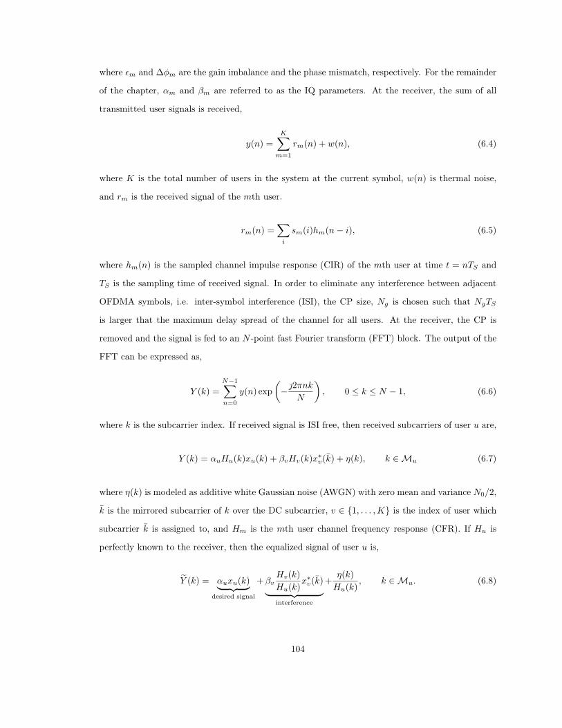
where εm and ∆φm are the gain imbalance and the phase mismatch, respectively. For the remainder
of the chapter, αm and βm are referred to as the IQ parameters. At the receiver, the sum of all
transmitted user signals is received,
y(n) =
K∑
m=1
rm(n) + w(n), (6.4)
where K is the total number of users in the system at the current symbol, w(n) is thermal noise,
and rm is the received signal of the mth user.
rm(n) =∑
i
sm(i)hm(n − i), (6.5)
where hm(n) is the sampled channel impulse response (CIR) of the mth user at time t = nTS and
TS is the sampling time of received signal. In order to eliminate any interference between adjacent
OFDMA symbols, i.e. inter-symbol interference (ISI), the CP size, Ng is chosen such that NgTS
is larger that the maximum delay spread of the channel for all users. At the receiver, the CP is
removed and the signal is fed to an N -point fast Fourier transform (FFT) block. The output of the
FFT can be expressed as,
Y (k) =
N−1∑
n=0
y(n) exp
(− 2πnk
N
), 0 ≤ k ≤ N − 1, (6.6)
where k is the subcarrier index. If received signal is ISI free, then received subcarriers of user u are,
Y (k) = αuHu(k)xu(k) + βvHv(k)x∗v(k) + η(k), k ∈ Mu (6.7)
where η(k) is modeled as additive white Gaussian noise (AWGN) with zero mean and variance N0/2,
k is the mirrored subcarrier of k over the DC subcarrier, v ∈ {1, . . . ,K} is the index of user which
subcarrier k is assigned to, and Hm is the mth user channel frequency response (CFR). If Hu is
perfectly known to the receiver, then the equalized signal of user u is,
Y (k) = αuxu(k)︸ ︷︷ ︸desired signal
+βvHv(k)
Hu(k)x∗
v(k)
︸ ︷︷ ︸interference
+η(k)
Hu(k), k ∈ Mu. (6.8)
104

It can be seen from the above equation that the first term is the desired signal with an attenuation
αu, the second term represents the ICI for v = u or the MUI for v 6= u, and the last term represents
the noise. The interference term can be canceled by jointly detecting xu(k) and x∗v(k). In such a
case, the receiver needs to estimate Hm for m = 1, . . . ,K. The pilot subcarriers Np are divided
among users/subchannels.
In an IQ distortion free OFDMA system, the system estimates the channel response at Nu
subcarriers using Np pilots. However, for a system suffering from IQ distortion, every user m
transmitting over subcarriers k ∈ Mm causes interference at k as well, as shown in (6.7). This
means that in worst case scenario, where k /∈ Mm∀k, the user effectively transmits over twice the
number of assigned subcarriers. Receiver then needs to estimate two user channels per subcarrier or
a total of 2Nu channel responses using the same number of pilots. In addition, estimation of K sets
of IQ parameters {αm, βm} is needed to fully cancel the interference introduced by image carriers
as shown in (6.8).
6.3 Channel/IQ Equalization
In this section, equalization of the channel effects and IQ distortions in the received signal is dis-
cussed. First, the UL frame structure needs to be introduced. In OFDMA systems, used subcarriers
are divided into smaller units, also known as tiles or chunks, which represent the minimum allocation
unit (see Fig. 6.1). The tiles are then assigned to subchannels either randomly or depending on user
channels. The overall received UL frame is a sum of all current user signals, which are transmitted
over different communication channels. The use of sophisticated channel estimation algorithms at
the receiver can significantly increase the system complexity and processing delay. Therefore, pi-
lots are assigned within each tile. The receiver can then perform channel estimation on each tile
individually using low complexity channel estimation techniques such as bilinear interpolation.
An example of how the UL frame is divided into tiles is shown in Fig. 6.1. Used subcarriers are
divided into Q tiles, with equal number of tiles on each side of the DC subcarrier. This means that for
every tile q, there is an image tile q = Q−q+1. Three different tile structures are shown in the figure,
where one tile dimensions are three symbols by four subcarriers. The tile bandwidth, Btile = 3∆f ,
where ∆f is the subcarrier spacing, and the tile duration, Ttile = 3Tsym, where Tsym = (N + Ng)TS
is the symbol duration. For the remainder of this chapter, Tile C structure is used. Note that a
105
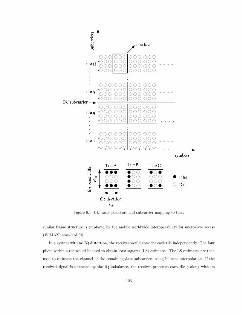
�������
��� ¡¢£¤¢�
¥¦��§¨©§©ª¦�« ¬ ª¦�« ª¦�« ®
�¯« §¦�«
§¦�« °±²©§¦�¯³µ¶·¸¹£º¤�¡»¼½£¼¹¾ ¿ ÀÁÂÃÄ
¨® �±�Å©²²¦«²§¦�« Ƨ¦�« Ç
§¦�« ȧ¦�« Æ
Figure 6.1 UL frame structure and subcarrier mapping to tiles.
similar frame structure is employed by the mobile worldwide interoperability for microwave access
(WiMAX) standard [9].
In a system with no IQ distortion, the receiver would consider each tile independently. The four
pilots within a tile would be used to obtain least squares (LS) estimates. The LS estimates are then
used to estimate the channel at the remaining data subcarriers using bilinear interpolation. If the
received signal is distorted by the IQ imbalance, the receiver processes each tile q along with its
106
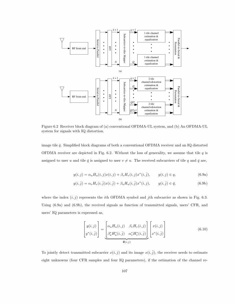
RF front-end
Parallel-to
-Serial &
Perm
uta
tion
FF
T
Serial-to
-Parallel
Su
bcarriers-to
-tiles Map
per
1-tile channel
estimation &
equalization
k = 1
N
q = 1
Q
1-tile channel
estimation &
equalization
(a)
RF front-end
Parallel-to
-Serial &
Perm
utatio
n
FF
T
Serial-to
-Parallel
Su
bcarriers-to
-tiles Map
per
2-tile
channel+distortion
estimation &
equalization
k = 1
N
q = 1
Q
(b)
Q/2
Q/2+1
2-tile
channel+distortion
estimation &
equalization
Figure 6.2 Receiver block diagram of (a) conventional OFDMA-UL system, and (b) An OFDMA-ULsystem for signals with IQ distortion.
image tile q. Simplified block diagrams of both a conventional OFDMA receiver and an IQ distorted
OFDMA receiver are depicted in Fig. 6.2. Without the loss of generality, we assume that tile q is
assigned to user u and tile q is assigned to user v 6= u. The received subcarriers of tile q and q are,
y(i, j) = αuHu(i, j)x(i, j) + βvHv(i, j)x∗(i, j), y(i, j) ∈ q, (6.9a)
y(i, j) = αvHv(i, j)x(i, j) + βuHu(i, j)x∗(i, j), y(i, j) ∈ q, (6.9b)
where the index (i, j) represents the ith OFDMA symbol and jth subcarrier as shown in Fig. 6.3.
Using (6.9a) and (6.9b), the received signals as function of transmitted signals, users’ CFR, and
users’ IQ parameters is expressed as,
y(i, j)
y∗(i, j)
=
αuHu(i, j) βvHv(i, j)
β∗uH∗
u(i, j) α∗vH∗
v (i, j)
︸ ︷︷ ︸Z(i,j)
x(i, j)
x∗(i, j)
(6.10)
To jointly detect transmitted subcarrier x(i, j) and its image x(i, j), the receiver needs to estimate
eight unknowns (four CFR samples and four IQ parameters), if the estimation of the channel re-
107
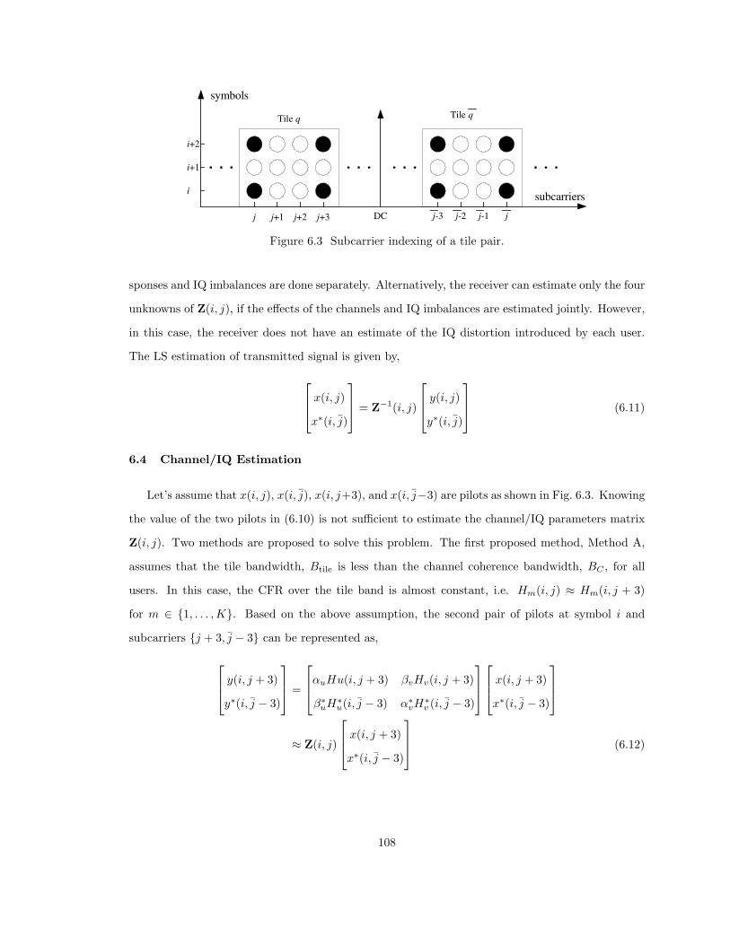
symbols
subcarriers
j j+1 j+2 j+3 j-3 j-2 j-1 j
i
i+1
i+2
Tile q Tile q
DC
Figure 6.3 Subcarrier indexing of a tile pair.
sponses and IQ imbalances are done separately. Alternatively, the receiver can estimate only the four
unknowns of Z(i, j), if the effects of the channels and IQ imbalances are estimated jointly. However,
in this case, the receiver does not have an estimate of the IQ distortion introduced by each user.
The LS estimation of transmitted signal is given by,
x(i, j)
x∗(i, j)
= Z−1(i, j)
y(i, j)
y∗(i, j)
(6.11)
6.4 Channel/IQ Estimation
Let’s assume that x(i, j), x(i, j), x(i, j+3), and x(i, j−3) are pilots as shown in Fig. 6.3. Knowing
the value of the two pilots in (6.10) is not sufficient to estimate the channel/IQ parameters matrix
Z(i, j). Two methods are proposed to solve this problem. The first proposed method, Method A,
assumes that the tile bandwidth, Btile is less than the channel coherence bandwidth, BC , for all
users. In this case, the CFR over the tile band is almost constant, i.e. Hm(i, j) ≈ Hm(i, j + 3)
for m ∈ {1, . . . ,K}. Based on the above assumption, the second pair of pilots at symbol i and
subcarriers {j + 3, j − 3} can be represented as,
y(i, j + 3)
y∗(i, j − 3)
=
αuHu(i, j + 3) βvHv(i, j + 3)
β∗uH∗
u(i, j − 3) α∗vH∗
v (i, j − 3)
x(i, j + 3)
x∗(i, j − 3)
≈ Z(i, j)
x(i, j + 3)
x∗(i, j − 3)
(6.12)
108

Using (6.10) and (6.12), the system can solve for Z(i, j). The same procedure is then repeated for
the two pilot pairs at symbol i + 2 to obtain Z(i + 2, j). To insure that this set of equations has a
unique solution, pilot vector pairs are chosen to be orthogonal [128, 129] such that,
[x(i, j) x∗(i, j)
]
x(i, j + 3)
x∗(i, j − 3)
= 0, (6.13a)
[x(i + 2, j) x∗(i + 2, j)
]
x(i + 2, j + 3)
x∗(i + 2, j − 3)
= 0. (6.13b)
Next, Z(i + 1, j) can be estimated using 1-D interpolation between Z(i, j) and Z(i + 2, j). Finally,
using (6.11), {Z(i, j),Z(i + 1, j),Z(i + 2, j)} are used to estimate the remaining data subcarriers at
symbols {i, i + 1, i + 2}, in this order. The receiver repeats this process for each pair of tiles (Q/2
times).
The second proposed method, Method B, assumes that the tile duration, Ttile is less than the
coherence time of the channel, TC , for all users. In this case, Hm(i, j) ≈ Hm(i + 2, j) for m ∈
{1, . . . ,K}. Based on the above assumption, the second pair of pilots (to be coupled with (6.10)) at
symbols {i, i + 2} and subcarriers {j, j} can be represented as,
y(i + 2, j)
y∗(i + 2, j)
≈ Z(i, j)
x(i + 2, j)
x∗(i + 2, j)
(6.14)
Using (6.10) and (6.14), the system solves for Z(i, j). Similarly, the pilot pairs at subcarriers
{j + 3, j − 3} can be used to solve for Z(i, j + 3). Next, the receiver uses linear interpolation to
calculate {Z(i, j + 1),Z(i, j + 2)} from {Z(i, j),Z(i, j + 3)}. Finally, the above values of Z are used
to estimate the remaining data subcarriers in both tiles. The procedure is then repeated for each
pair of tiles. The pilots orthogonality is achieved as follows,
[x(i, j) x∗(i, j)
]
x(i + 2, j)
x∗(i + 2, j)
= 0, (6.15a)
[x(i, j + 3) x∗(i, j − 3)
]
x(i + 2, j + 3)
x∗(i + 2, j − 3)
= 0. (6.15b)
109
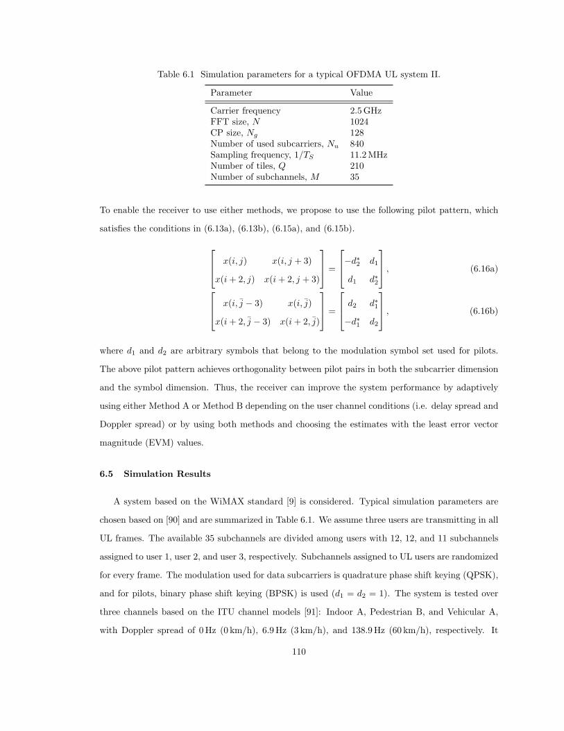
Table 6.1 Simulation parameters for a typical OFDMA UL system II.
Parameter Value
Carrier frequency 2.5 GHzFFT size, N 1024CP size, Ng 128Number of used subcarriers, Nu 840Sampling frequency, 1/TS 11.2 MHzNumber of tiles, Q 210Number of subchannels, M 35
To enable the receiver to use either methods, we propose to use the following pilot pattern, which
satisfies the conditions in (6.13a), (6.13b), (6.15a), and (6.15b).
x(i, j) x(i, j + 3)
x(i + 2, j) x(i + 2, j + 3)
=
−d∗2 d1
d1 d∗2
, (6.16a)
x(i, j − 3) x(i, j)
x(i + 2, j − 3) x(i + 2, j)
=
d2 d∗1
−d∗1 d2
, (6.16b)
where d1 and d2 are arbitrary symbols that belong to the modulation symbol set used for pilots.
The above pilot pattern achieves orthogonality between pilot pairs in both the subcarrier dimension
and the symbol dimension. Thus, the receiver can improve the system performance by adaptively
using either Method A or Method B depending on the user channel conditions (i.e. delay spread and
Doppler spread) or by using both methods and choosing the estimates with the least error vector
magnitude (EVM) values.
6.5 Simulation Results
A system based on the WiMAX standard [9] is considered. Typical simulation parameters are
chosen based on [90] and are summarized in Table 6.1. We assume three users are transmitting in all
UL frames. The available 35 subchannels are divided among users with 12, 12, and 11 subchannels
assigned to user 1, user 2, and user 3, respectively. Subchannels assigned to UL users are randomized
for every frame. The modulation used for data subcarriers is quadrature phase shift keying (QPSK),
and for pilots, binary phase shift keying (BPSK) is used (d1 = d2 = 1). The system is tested over
three channels based on the ITU channel models [91]: Indoor A, Pedestrian B, and Vehicular A,
with Doppler spread of 0 Hz (0 km/h), 6.9 Hz (3 km/h), and 138.9 Hz (60 km/h), respectively. It
110
is assumed that the channel is independent between different frames and between different users.
The receiver processes each frame individually. At the receiver, the uncoded bit error rate (BER) is
measured and averaged over all users.
For all generated simulations, it is first assumed that there are no IQ imbalances introduced to
the signal. The receiver uses all pilots per tile to estimate and equalize only the channel effects
using 2-D linear interpolation technique. This case is labeled as “Ideal IQ”. Next, the UL user
signals are distorted by IQ imbalances. The IQ gain imbalance and phase mismatch of user 1,
user 2, and user 3 are {0.2, 2◦}, {0.35, 5◦}, and {0.5, 8◦}, respectively. The uncoded BER is
measured while the receiver operates assuming no IQ imbalance is present. The results are labeled
as “IQ Imbalance/ No compensation”. Finally, Method A and Method B are used to estimate and
equalize the combined channel and IQ distortions. The results are shown in Fig. 6.4, Fig. 6.5, and
Fig. 6.6. In all figures, the system performance degrades significantly when the receiver ignores the
IQ distortions to the signal. At a signal-to-noise ratio (SNR) of 35 dB, the IQ distortions increase
the BER by two orders of magnitude. On the other hand, proposed methods manage to reduce the
BER considerably. For the results over the Pedestrian B channel in Fig. 6.4, the delay spread is high
while the Doppler spread is low. As a result, Method B outperforms Method A, since it assumes
low Doppler spreading. Method B significantly reduces the IQ distortion effect on the signal. The
loss is around 2 dB from the ideal IQ case at BER = 10−3. For the results over the Vehicular A
channel in Fig. 6.5, both delay spread and Doppler spread are high. In this case, Method A slightly
outperforms Method B, since its approximation is more accurate. While both methods A and B
improve the BER significantly, the loss from the ideal IQ case is considerable. Under such highly
selective channels and with IQ distortions, the system can choose to reduce signal bandwidth which
leads to an improved performance of Method A. Finally, for the results over the Indoor A channel in
Fig. 6.6, both delay spread and Doppler spread are low. As expected in this case, both methods A
and B perform very well. The BER degradation due to the IQ distortions is recovered with around
2.5 dB loss from the ideal IQ case at BER = 10−3. Note that there is a loss from the ideal IQ
case even in channels with low Doppler spread and delay spread. This loss is a result of the noise
averaging effect. In ideal case, the estimation of channel response, which is almost constant over slot
bandwidth and/or slot duration, is averaged by the bilinear interpolation over twice the number of
pilots compared to proposed methods. A receiver capable of detecting the presence of IQ distortions
111
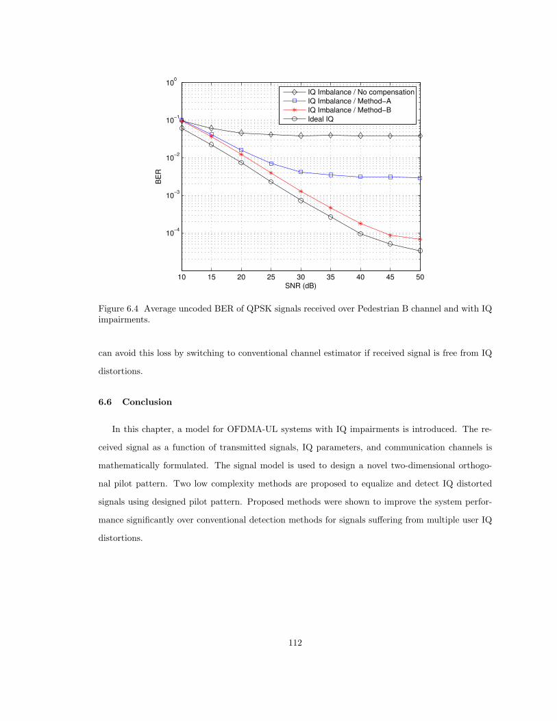
10 15 20 25 30 35 40 45 50
10−4
10−3
10−2
10−1
100
SNR (dB)
BE
R
IQ Imbalance / No compensation
IQ Imbalance / Method−A
IQ Imbalance / Method−B
Ideal IQ
Figure 6.4 Average uncoded BER of QPSK signals received over Pedestrian B channel and with IQimpairments.
can avoid this loss by switching to conventional channel estimator if received signal is free from IQ
distortions.
6.6 Conclusion
In this chapter, a model for OFDMA-UL systems with IQ impairments is introduced. The re-
ceived signal as a function of transmitted signals, IQ parameters, and communication channels is
mathematically formulated. The signal model is used to design a novel two-dimensional orthogo-
nal pilot pattern. Two low complexity methods are proposed to equalize and detect IQ distorted
signals using designed pilot pattern. Proposed methods were shown to improve the system perfor-
mance significantly over conventional detection methods for signals suffering from multiple user IQ
distortions.
112
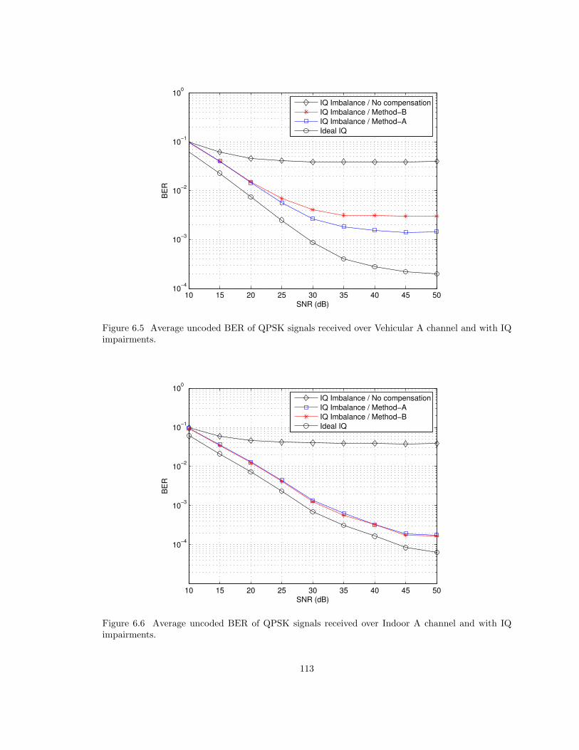
10 15 20 25 30 35 40 45 5010
−4
10−3
10−2
10−1
100
SNR (dB)
BE
R
IQ Imbalance / No compensation
IQ Imbalance / Method−B
IQ Imbalance / Method−A
Ideal IQ
Figure 6.5 Average uncoded BER of QPSK signals received over Vehicular A channel and with IQimpairments.
10 15 20 25 30 35 40 45 50
10−4
10−3
10−2
10−1
100
SNR (dB)
BE
R
IQ Imbalance / No compensation
IQ Imbalance / Method−A
IQ Imbalance / Method−B
Ideal IQ
Figure 6.6 Average uncoded BER of QPSK signals received over Indoor A channel and with IQimpairments.
113
CHAPTER 7
ERROR VECTOR MAGNITUDE BASED SNR ESTIMATION IN BLINDRECEIVERS
7.1 Introduction
In wireless communication systems, complex digital modulation schemes are used for meeting
stringent spectral and signal-to-noise ratio (SNR) requirements [130]. In such systems, the overall
quality of the transmission and reception are determined by various baseband and RF system spec-
ifications. Among these, bit error rate (BER) and error vector magnitude (EVM) are two primary
specifications that determine the performance of the wireless system in terms of transmitted and
received symbols corresponding to a given digital modulation scheme. While BER is useful as a con-
ceptual figure of merit, it suffers from a number of practical drawbacks that compromise its value
as a standard test in manufacturing or maintenance [131]. Calculation of BER requires dedicated
equipment, thus increasing the cost and complexity of the test system. In addition, it has limited
diagnostic value. If the BER value measured exceeds accepted limits, it offers no clue regarding the
probable cause or source of signal degradation.
For measurements and testing devices, EVM is a viable alternative test method when looking
for a figure of merit in non-regenerative transmission links. EVM can offer insightful information
on the various transmitter imperfections, including carrier leakage, IQ mismatch, nonlinearity, lo-
cal oscillator (LO) phase noise and frequency error [19]. Requirements on EVM are already part
of most wireless communications standards such as the IEEE 802.11a-1999 standard [6] and the
IEEE 802.16e-2005 worldwide interoperability for microwave access (WiMAX) standard [9]. EVM
measurements and simulations can be found in [131–133]. The impact of IQ imbalance, as well as
LO phase noise on EVM is investigated in [134] and EVM as a function of these impairments is
derived. This work has been expanded in [19], where the effects of carrier leakage, nonlinearity and
LO frequency error on EVM are considered.
114
Relating EVM to other performance metrics such as SNR and BER is an important research
topic, as well [135, 136]. These relations are quite useful since it allows the reuse of already available
EVM measurements to infer more information regarding the communication system. Moreover, using
EVM measurements could reduce the system complexity by getting rid of the need to have separate
modules to estimate or measure other metrics. When relating EVM to SNR, one assumption that
has been made is that the EVM is measured using known data sequences (e.g. preambles or pilots)
or that the SNR is high enough that symbol errors are negligible [135, 136]. Another assumption
was that one or two system imperfections are dominant; the remaining imperfections are modeled
as Gaussian noise [19, 134]. However, the above analyses did not consider measuring EVM blindly
for low SNR levels where symbol errors are possible. With new technologies for spectrum detection
and utilization [4, 92], there is a need to detect signals at medium to very low SNR values. The
signal quality metrics including EVM and SNR are possibly measured over unknown data sequences
(nondata-aided) as well.
In this chapter, we consider the relation between EVM and SNR for nondata-aided receivers.
The signal degradation sources are modeled as additive white Gaussian noise (AWGN), Rayleigh
fading channels, and IQ imbalances. It is shown that for higher modulation orders or low SNR
values, using previously made assumptions leads to inaccurate results. The exact value of EVM for
nondata-aided symbol detection is derived and expressed in terms of the SNR. The derived relations
are then used to estimate the SNR using measured EVM values for QAM and PAM signals and over
limited number of symbols. The results show that SNR can be accurately estimated using measured
EVM even when symbol sequences are unknown, and the SNR level is low.
The remainder of this chapter is organized as follows. In Section 7.2, the signal model and
assumptions are presented. The EVM is defined and mathematically expressed in Section 7.3.
Relation between EVM and SNR for data-aided receivers and its application to nondata-aided
receivers are discussed in Section 7.4. In Section 7.5, the EVM relation to SNR is derived for QAM
and PAM signals. Computer-based simulations are performed to examine the correctness of derived
expressions; those results are discussed in Section 7.6. Finally, concluding remarks are given in
Section 7.7.
115
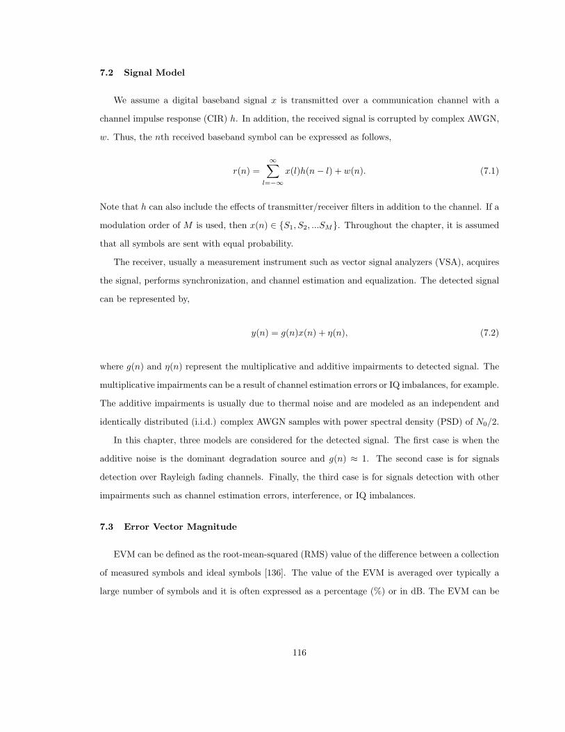
7.2 Signal Model
We assume a digital baseband signal x is transmitted over a communication channel with a
channel impulse response (CIR) h. In addition, the received signal is corrupted by complex AWGN,
w. Thus, the nth received baseband symbol can be expressed as follows,
r(n) =
∞∑
l=−∞x(l)h(n − l) + w(n). (7.1)
Note that h can also include the effects of transmitter/receiver filters in addition to the channel. If a
modulation order of M is used, then x(n) ∈ {S1, S2, ...SM}. Throughout the chapter, it is assumed
that all symbols are sent with equal probability.
The receiver, usually a measurement instrument such as vector signal analyzers (VSA), acquires
the signal, performs synchronization, and channel estimation and equalization. The detected signal
can be represented by,
y(n) = g(n)x(n) + η(n), (7.2)
where g(n) and η(n) represent the multiplicative and additive impairments to detected signal. The
multiplicative impairments can be a result of channel estimation errors or IQ imbalances, for example.
The additive impairments is usually due to thermal noise and are modeled as an independent and
identically distributed (i.i.d.) complex AWGN samples with power spectral density (PSD) of N0/2.
In this chapter, three models are considered for the detected signal. The first case is when the
additive noise is the dominant degradation source and g(n) ≈ 1. The second case is for signals
detection over Rayleigh fading channels. Finally, the third case is for signals detection with other
impairments such as channel estimation errors, interference, or IQ imbalances.
7.3 Error Vector Magnitude
EVM can be defined as the root-mean-squared (RMS) value of the difference between a collection
of measured symbols and ideal symbols [136]. The value of the EVM is averaged over typically a
large number of symbols and it is often expressed as a percentage (%) or in dB. The EVM can be
116
represented as [137],
EVMRMS =
√√√√√√1
N
N∑
n=1
|Sr(n) − St(n)|2
P0, (7.3)
where N is the number of symbols over which the value of EVM is measured, Sr(n) is the normalized
received nth symbol which is corrupted by Gaussian noise, St(n) is the ideal/transmitted value of the
nth symbol x(n), and P0 is either the maximum normalized ideal symbol power or the average power
of all symbols for the chosen modulation. For the remainder of this chapter, the latter definition of
P0 is used. In such case,
P0 =1
M
M∑
m=1
|Sm|2. (7.4)
The EVM value is normalized with the average symbol energy to remove the dependency of EVM on
the modulation order. In (7.3), Sr(n) is the detected symbol y(n) and St(n) could be either known
to the receiver (data-aided) if pilots or preambles are used to measure the EVM, or estimated from
y(n) (nondata-aided) if data symbols are used instead.
7.4 Relating EVM to SNR
Let us consider the case where the signal is only corrupted by AWGN. For data-aided EVM
calculations, (7.3) is reduced to,
EVMRMS =
√√√√√√1
N
N∑
n=1
|η(n)|2
P0. (7.5)
If the EVM is measured over large values of N , then [135, 136, 138],
EVMRMS ≈√
N0
P0=
√1
SNR, (7.6)
where N0/2 = σ2n is the noise PSD.
The above EVM-SNR relation, however, only holds for data-aided receivers. For nondata-aided
receivers, the transmitted symbols are estimated and those estimates x(n) are used to measure the
117
EVM value. Thus, for low SNR values, errors are made when estimating x(n). The measured EVM
value in this case is expected to be less than its actual value as the symbol estimator tends to
assign received symbols to their closest possible constellation point. For a BPSK signal, the symbol
estimator criterion is as follows,
x(n) =
S1, if y<(n) > 0,
S2, if y<(n) < 0,
(7.7)
where y<(n) is the real part of y(n). Note that for y<(n) = 0, x(n) = S1 or S2 with equal probability.
As such, errors in estimating x(n), and consequently in measuring the EVM, occurs every time a
constellation point passes to another point decision region. To further illustrate the effect of such
errors on the EVM-SNR relation, the EVM versus SNR curves for various modulation orders are
plotted in Fig. 7.1. The results are averaged over 100, 000 modulated symbols. The ideal value of
EVM (= 1/√
SNR) is also plotted for reference. Two observations can be drawn from this figure.
First, the measured EVM values are less than the ideal EVM, as expected. Second, the measured
EVM deviation from its ideal value increases with the modulation order. This is due to the fact
that for higher modulation orders, and for the same SNR level, the probability of a symbol error is
higher [89],
PS = 1 −[2
(1 − 1√
M
)Q
(√3
M − 1SNR
)]2
, (7.8)
where PS is the symbol error rate (SER), M is the modulation order, Q(v) = 1/2 erfc(v/√
2), and
erfc(·) is the complementary error function. Note that the above equation holds for QAM signals
but not for BPSK signals. Based on the above, the measured EVM for nondata-aided receivers
becomes dependent on the modulation order even with the normalization in (7.3). Moreover, using
the measured EVM as an indication of the SNR as in (7.6) can be misleading, especially for low SNR
levels. Thus, there is a need for a more accurate EVM to SNR relation for nondata-aided receivers.
118
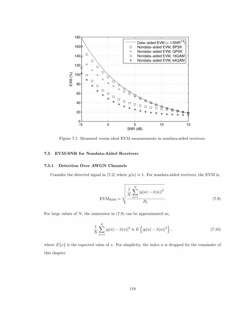
−5 0 5 10 150
20
40
60
80
100
120
140
160
180
SNR (dB)
EV
M (
%)
Data−aided EVM (= 1/SNR1/2
)
Nondata−aided EVM, BPSK
Nondata−aided EVM, QPSK
Nondata−aided EVM, 16QAM
Nondata−aided EVM, 64QAM
Figure 7.1 Measured versus ideal EVM measurements in nondata-aided receivers.
7.5 EVM-SNR for Nondata-Aided Receivers
7.5.1 Detection Over AWGN Channels
Consider the detected signal in (7.2) where g(n) ≈ 1. For nondata-aided receivers, the EVM is,
EVMRMS =
√√√√√√1
N
N∑
n=1
|y(n) − x(n)|2
P0. (7.9)
For large values of N , the numerator in (7.9) can be approximated as,
1
N
N∑
n=1
|y(n) − x(n)|2 ≈ E{|y(n) − x(n)|2
}, (7.10)
where E{x} is the expected value of x. For simplicity, the index n is dropped for the remainder of
this chapter.
119
We first start by considering BPSK signals. In this case, x and x are real signals. Thus, we can
rewrite (7.10) as follows,
E{|y − x|2
}= E
{(y< − x)
2}
+ E{η2=}
, (7.11)
where y< = x+ η<, and the subscripts < and = represent the real and imaginary components of the
signal, respectively. Note that η< and η= are uncorrelated random processes that have a Gaussian
distribution with zero mean and σ2n variance. Thus,
E{η2=}
= σ2n. (7.12)
To evaluate E{(y< − x)2}, the statistical properties of y< is examined. Since BPSK modulation
is considered, then x ∈ {−a, a}, where a is the symbol amplitude. Thus, the conditional probability
density function (PDF) of received signal is,
f(y<|x = Si) =1
σnφ
(y< − Si
σn
), (7.13)
where,
φ(v) =1√2π
exp
(−v2
2
)(7.14)
and φ(·) the PDF of a standard normal distribution. Based on the criterion in (7.7), the probability
of x = a is,
P (x = a) = P (x = −a)
∫ ∞
0
f(y<|x = −a) dy< + P (x = a)
∫ ∞
0
f(y<|x = a) dy<. (7.15)
It is assumed that,
P (x = −a) = P (x = a) =1
2. (7.16)
As such, it can be shown that,
f(y<|x = a) =1
C
(f(y<|x = −a) + f(y<|x = a)
), y< > 0, (7.17)
120

and
f(y<|x = −a) =1
C
(f(y<|x = −a) + f(y<|x = a)
), y< < 0, (7.18)
where C is a constant chosen such that,
∫ ∞
−∞f(y<|x = Si) dy< = 1. (7.19)
In this case, C = 1. Using (7.17) and (7.18),
E{(y< − x)2
}= P (x = −a)
∫ ∞
−∞(y< + a)2f(y<|x = −a) dy<
+ P (x = a)
∫ ∞
−∞(y< − a)2f(y<|x = a) dy<. (7.20)
Since the decision point (y< = 0) is equally spaced between the two possible values of x and since
f(y<|x = Si) is symmetric around x, then,
P (x = −a) = P (x = a) =1
2. (7.21)
Since f(y<|x = −a) = f(−y<|x = a), then by exchanging y< with −y< in the second integral
in (7.20) and with some manipulation it can be shown that,
∫ ∞
−∞(y< + a)2f(y<|x = −a) dy< =
∫ ∞
−∞(y< − a)2f(y<|x = a) dy<. (7.22)
Thus, using (7.21) and (7.22), (7.20) can be reduced to,
E{(y< − x)2
}=
∫ ∞
−∞(y< − a)2f(y<|x = a) dy<. (7.23)
From (7.18) and (7.13), the integral in (7.23) can be expressed as,
E{(y< − x)2
}=
1
σn
∫ ∞
0
(y< − a)2φ
(y< + a
σn
)dy< +
1
σn
∫ ∞
0
(y< − a)2φ
(y< − a
σn
)dy<,
=1
σn
∫ ∞
−a
v2φ
(v + 2a
σn
)dv +
1
σn
∫ ∞
−a
v2φ
(v
σn
)dv, (7.24)
121

where v = y< − a. The last two integrals in (7.24) are related to E{V 2} where V is a random
variable that has a low-truncated normal distribution [139]. To solve (7.24), we define a new function
z(A,µ, σ), where,
z(A,µ, σ) ≡ 1
σ
∫ ∞
A
v2φ
(v − µ
σ
)dv (7.25)
It is shown in Appendix C that,
z(A,µ, σ) = σ(A + µ)φ
(A − µ
σ
)+ (µ2 + σ2)Q
(A − µ
σ
)(7.26)
Using (7.25), the solution to (7.24) is,
E{(y< − x)2
}= z(−a,−2a, σn) + z(−a, 0, σn)
= −3aσnφ
(a
σn
)+ (4a2 + σ2
n)Q
(a
σn
)− aσnφ
(−a
σn
)+ σ2
nQ
(−a
σn
). (7.27)
Note that φ(v) = φ(−v) and Q(−v) + Q(v) = 1. As such, (7.27) is reduced to,
E{(y< − x)2
}= σ2
n − 4aσnφ
(a
σn
)+ 4a2Q
(a
σn
)(7.28)
Then, substituting (7.28) and (7.12) into (7.11),
E{|y − x|2
}= 2σ2
n − 4aσnφ
(a
σn
)+ 4a2Q
(a
σn
). (7.29)
Without the loss of generality, we assume that the average symbol power, P0 = 1 (i.e. a = 1).
Therefore
SNR =P0
N0=
1
2σ2n
. (7.30)
To relate EVM to SNR for nondata-aided receivers and for BPSK signaling, the results from (7.29),
(7.30) are substituted into (7.9) as follows,
EVMBPSK =
[1
SNR− 4√
2SNRφ(√
2SNR)
+ 4Q(√
2SNR)]1/2
, (7.31)
122
or more conveniently using the exponential and error functions as,
EVMBPSK =
[1
SNR− 2√
πSNRexp(−SNR) + 2 erfc
(√SNR
)]1/2
. (7.32)
Note that the first square-rooted term in (7.32) represents the ideal EVM value. The second and
last terms represent the errors caused by the symbol estimation process. For high values of SNR, the
last two terms converge to zero and the EVM approaches its ideal value. This is explained by the
fact that for high SNR values, the probability of symbol error goes to zero. This is also confirmed
by the simulation results in Fig. 7.1. The validity of (7.32) is further investigated in Section 7.6.
Next, we consider square QAM signals (i.e. with even number of bits per symbol such as QPSK,
16QAM, 64QAM, etc). For a QAM signal of order M , the modulated symbols are,
x = (2i − k)a + (2m − k)a, i,m = 0, 1, . . . , k (7.33)
where k =√
M − 1. In this case,
E{|y − x|2} = E{(y< − x<)2} + E{(y= − x=)2}. (7.34)
Due to the independence and symmetry between the real and imaginary parts of the signal, E{(y<−
x<)2} = E{(y= − x=)2}. Thus, it is sufficient to calculate only one of the above expectations. For
non-square QAM signals, the above equality does not hold. It is shown later in this section how to
calculate the expected EVM value in such case.
In the following analysis, the real part of the signal is considered. Generalizing the expression
in (7.20), E{(y< − x<)2} can be obtained by averaging over all possible values of x< as follows,
E{(y< − x<)2} =
k∑
i=0
P (x< = Si)E{(y< − Si)2|x< = Si}
=
k∑
i=0
P (x< = Si)
∫ ∞
−∞(y< − Si)
2f(y<|x< = Si)dy<, (7.35)
123

where Si = (2i−k)a, is the real value of the modulation symbol. Similar to (7.17), it be shown that
for any arbitrary value of i,
f(y<|x< = Si) =1
Ci
k∑
j=0
f(y<|x< = Sj)
, y< ∈ Di
=1
Ci
k∑
j=0
1
σnφ
(y< − Sj
σn
) , y< ∈ Di (7.36)
where Di is the decision region for symbol Si such that,
for i = 0, −∞ <D0 ≤ S0 + a,
for 1 ≤i ≤ k − 1, Si − a <Di ≤ Si + a,
and for i = k, Sk − a <Dk < ∞. (7.37)
To satisfy the condition in (7.19), the normalization constant Ci is found to be,
Ci =
∫
Di
k∑
j=0
1
σnφ
(y< − Sj
σn
)dy<,
=
k∑
j=0
∫
Di
1
σnφ
(y< − Sj
σn
)dy<, (7.38)
where the integral and summation in (7.38) are interchangeable. On the other hand, P (x< = Si)
can be evaluated as follows,
P (x< = Si) =k∑
j=0
P (x< = Sj)
∫
Di
1
σnφ
(y< − Sj
σn
)dy<. (7.39)
It is assumed that all modulation symbols are transmitted with equal probability such that P (x< =
Sj) = 1/(k + 1), ∀j. From the above, (7.39) becomes,
P (x< = Si) =1
k + 1
k∑
j=0
∫
Di
1
σnφ
(y< − Sj
σn
)dy<. (7.40)
124
From (7.38) and (7.40), it can be seen that P (x< = Si) = Ci/(k + 1). Thus, using (7.36), (7.38),
and (7.40), the expression in (7.35) is reduced to,
E{(y< − x<)2} =1
k + 1
k∑
i=0
k∑
j=0
∫
Di
1
σn(y< − Si)
2φ
(y< − Sj
σn
)dy<, (7.41)
By using v = y< − Si,
E{(y< − x<)2} =1
k + 1
k∑
i=0
k∑
j=0
∫
Di
v2
σnφ
(v − µji
σn
)dv
︸ ︷︷ ︸Iji
(7.42)
where Di = Di − Si and µji = 2a(j − i) = Sj − Si. To evaluate the integral in (7.42) Iji, we need
to consider two cases. The first case is the singly-truncated decision regions (i.e. i = 0, k), and the
second case is the doubly-truncated decision regions (i.e. 1 ≤ i ≤ k − 1). Due to the symmetry
around zero, the values of Iji are equal for i = 0 and i = k (or generally for any i and k − i). Thus,
Ij0 = Ijk =1
σn
∫ ∞
−a
v2φ
(v − µjk
σn
)dv
= z(−a, µjk, σn). (7.43)
For doubly-truncated regions,
Iji =
∫ a
−a
v2φ
(v − µji
σn
)dv
= z(−a, µji, σn) − z(a, µji, σn), 1 ≤ i ≤ k − 1. (7.44)
Substituting (7.43) and (7.44) into (7.42),
E{(y< − x<)2} =1
k + 1
2
k∑
j=0
z(−a, µjk, σn) +
k−1∑
i=1
k∑
j=0
[z(−a, µji, σn) − z(a, µji, σn)
] . (7.45)
It is shown in Appendix D that (7.45) reduces to,
E{(y< − x<)2} = σ2n − 8aσn
k∑
i=1
γiφ
[βia
σn
]+ 8a2
k∑
i=1
γiβiQ
[βia
σn
], (7.46)
125
where
γi = 1 − i
k + 1, and βi = 2i − 1. (7.47)
Combining (7.30), (7.34), and (7.46), and exchanging φ and Q with the exponential and error
functions,
E{|y − x|2} =1
SNR− 8a√
πSNR
k∑
i=1
γi exp(−β2i a2SNR) + 8a2
k∑
i=1
γiβi erfc(βia
√SNR
). (7.48)
For a normalized QAM system,
a =
√3
2(M − 1). (7.49)
From (7.9), (7.48), and (7.49), the EVM for QAM signals is
EVMQAM =
[1
SNR− 8
√3
2π(M − 1)SNR
√M−1∑
i=1
γi exp
(− 3β2
i SNR
2(M − 1)
)
+12
(M − 1)
√M−1∑
i=1
γiβi erfc
(√3β2
i SNR
2(M − 1)
)]1/2
, (7.50)
where
γi = 1 − i√M
, and βi = 2i − 1. (7.51)
In view of the above results, some remarks are in order. First, similar to the EVM of a BPSK signal
in (7.32), the EVM of a QAM signal in (7.50) can be divided into two parts. The first part is 1/SNR,
which represents the ideal EVM when no errors are introduced to the symbol detection. The second
part, which in QAM case is a sum of exponential and error functions, represents the reduction in
measured EVM due to detection error. The second error part is a function of both the modulation
order M and the SNR level, and it goes to zero for high values of SNR. Note that as the summation
index i in (7.50) increases, the value of the exponential and error functions decreases rapidly. Hence,
for high modulation order, an approximation of the EVM value can be obtained by considering only
the first few terms of the summations.
126
Second, the expression in (7.46) can be used to evaluate the EVM for QAM systems with odd
number of bits per symbol. In this case, the E{(y< − x<)2} and E{(y= − x=)2} are not equal.
Using (7.46), E{(y< − x<)2} and E{(y= − x=)2} can be evaluated for k = k1 − 1 and k = k2 − 1,
where M = k1k2, and k1 and k2 represents the number of constellation points on the real and
imaginary parts of the signal, respectively. Finally, the EVM can be evaluated by substituting the
above values into (7.34) and repeating a similar process to the one in (7.48) and (7.50).
Third, note that the EVM for a normalized PAM signal can be obtained from (7.46) by adding
σ2n, setting k to M − 1, and a to
√3/(M2 − 1), such that
EVMPAM =
[1
SNR− 4
√3
π(M2 − 1)SNR
M−1∑
i=1
γi exp
(− 3β2
i SNR
(M2 − 1)
)
+12
(M2 − 1)
M−1∑
i=1
γiβi erfc
(√3β2
i SNR
(M2 − 1)
)]1/2
, (7.52)
where
γi = 1 − i
M, and βi = 2i − 1. (7.53)
For example, by setting M = 2 in (7.52), the EVM for BPSK signals in (7.29) can be obtained.
7.5.2 Detection over Rayleigh Fading Channels
For signals detected over Rayleigh fading channels [89],
y(n) = α exp(−θ)x(n) + η(n), (7.54)
where α and θ are the attenuation and phase shift introduced by the fading channel, and α is a
Rayleigh-distributed random variable. Slow fading is assumed such that the channel response is
constant over at least one symbol interval. If the channel fading is sufficiently slow, the phase
shift θ can be estimated from the received signal without error. In this case, it can be shown that
the instantaneous SNR is chi-square-distributed [89]. To evaluate the average EVM value, we first
consider the instantaneous EVM value for a given α. In the following analysis, QAM signals are
127
considered. Thus, from (7.50), the instantaneous EVM is,
EVMQAM(α) =
[1
SNR− 8α
√3
2π(M − 1)SNR
√M−1∑
i=1
γi exp
(−3α2β2
i SNR
2(M − 1)
)
+12α2
(M − 1)
√M−1∑
i=1
γiβi erfc
(√3α2β2
i SNR
2(M − 1)
)]1/2
, (7.55)
where γi and βi are as in (7.51). The PDF of α is,
f(α) = 2α exp(−α2), α ≥ 0. (7.56)
The expected value of EVM is evaluated by averaging over α,
EVMQAM =
∫ ∞
0
EVMQAM(α)f(α)dα. (7.57)
The evaluation of the integral in (7.57) is skipped here for brevity. The EVM is found to be,
EVMQAM =
[1
SNR+
4
SNR2
√3
2(M − 1)
√M−1∑
i=1
γi
[3β2
i
2(M − 1)+
1
SNR
]−3/2
+12
(M − 1)
√M−1∑
i=1
γiβi
(1 −
√3β2
i SNR
2(M − 1) + 3β2i SNR
[1 +
(M − 1)
2(M − 1) + 3β2i SNR
])]1/2
(7.58)
7.5.3 Detection with Other Impairments
In the previous section, the effect of Rayleigh fading channels on the measured EVM of received
signals was considered. Since it was assumed that the phase shift caused by the channel can be
perfectly estimated from the received signal, there was no interference between the real and imaginary
parts of the signal. In this section, we consider the case where the multiplicative term, g(n) in (7.2),
can have a complex value that is unknown to the receiver. Since g(n) is complex-valued, there will
be interference between the real and imaginary parts of the signal. This case can be used to model
received signals with impairments such as the IQ imbalance [124] or channel estimation errors [114].
128

The received signal can be represented using its real and imaginary parts as
y<
y=
=
g11 g12
g21 g22
x<
x=
+
µ<
µ=
, (7.59)
where the index n is dropped to simplify the presentation. In the following, QAM signals are
considered. Assume the transmitted signal is as in (7.33). In this case, and for a given value of g,
the expected value of the real and imaginary parts of the detected signals are,
E{y<|i,m} = (2i − k)ag11 + (2m − k)ag12 ≡ µ<(i,m), (7.60)
E{y=|i,m} = (2i − k)ag21 + (2m − k)ag22 ≡ µ=(i,m). (7.61)
Ideally, the signal should be detected such that (g11 = g22) and (g12 = g21 = 0). The previous two
equalities are lost if the IQ modulator is suffering from gain and phase imbalances, respectively. In
this case, there is interference between the real and imaginary parts of x in the detected signal y.
Since it is assumed that g is unknown to the receiver, the decision regions are the same as in (7.37).
Following the same analysis presented in Section 7.5.1, similar results to (7.45) are obtained as
follow,
E{(y< − x<)2} =1
M
k∑
i=0
k∑
m=0
2z(−a, µ
(R)imk, σn) +
k−1∑
j=1
[z(−a, µ
(R)imj , σn) − z(a, µ
(R)imj , σn)
] , (7.62)
E{(y= − x=)2} =1
M
k∑
i=0
k∑
m=0
2z(−a, µ
(I)imk, σn) +
k−1∑
j=1
[z(−a, µ
(I)imj , σn) − z(a, µ
(I)imj , σn)
] , (7.63)
where
µ(R)imj = µ<(i,m) − (2j − k)a, (7.64)
µ(I)imj = µ=(i,m) − (2j − k)a. (7.65)
Note that in this case, the symmetry between the real and imaginary components of the detected
signal y is lost. Thus, to measure the final EVM value, expectations of both the real and imaginary
parts of the signal needs to be considered. The symmetry is restored if |g11| = |g22| and |g12| = |g21|.
In addition, due to the interference between the I and Q branches of the IQ modulator, the expected
129
value needs to be averaged over all possible values of the Q signal in addition to the I signal. Hence,
as compared to (7.45), the expressions in (7.62) and (7.63) contain an extra summation over m.
Further simplification of (7.62) and (7.63) is not possible since µ(R)imj and µ
(I)imj have distinctive values
for each set of i, m, and j (unlike µij in (7.45) whose values depend only on the difference i − j).
Finally, the average EVM can be evaluated as,
EVMQAM(g) =[E{(y< − x<)2} + E{(y= − x=)2}
]1/2. (7.66)
While g is usually considered constant such as in the case of IQ imbalances, in some other cases g
can be modeled as a random process. For example, channel estimation errors can be modeled as
a multiplicative random variable with Gaussian distribution [114]. In this case, the EVM expected
value can be obtained by averaging over the PDF of g similar to (7.57).
To examine the validity of the results present in (7.62) and (7.63), we consider the case where
the SNR is sufficiently high and g ≈ I such that the probability of a symbol detection error is zero,
where I is the identity matrix. This is equivalent to assuming that the transmitted sequence x(n) is
known to the receiver. In this case,
z(−a, µ(R)imk, σn) =
[µ
(R)kmk
]2+ σ2
n, for i = k
0, otherwise,
z(−a, µ(R)imj , σn) − z(a, µ
(R)imj , σn) =
[µ
(R)jmj
]2+ σ2
n, for i = j
0, otherwise,
(7.67)
Substituting (7.67) in (7.62) and (7.63), and assuming a normalized QAM signal, the EVM is found
to be,
EVMQAM (g) =
√1
SNR+ 1 +
1
2(g2
11 + g212 + g2
21 + g222) − (g11 + g22). (7.68)
It is conventional to assume, without the loss of generality, that the impairments matrix g is nor-
malized such that (g211 + g2
12 + g221 + g2
22 = 2). In this case,
EVMQAM (g) =
√1
SNR+ 2 − Tr(g), (7.69)
130
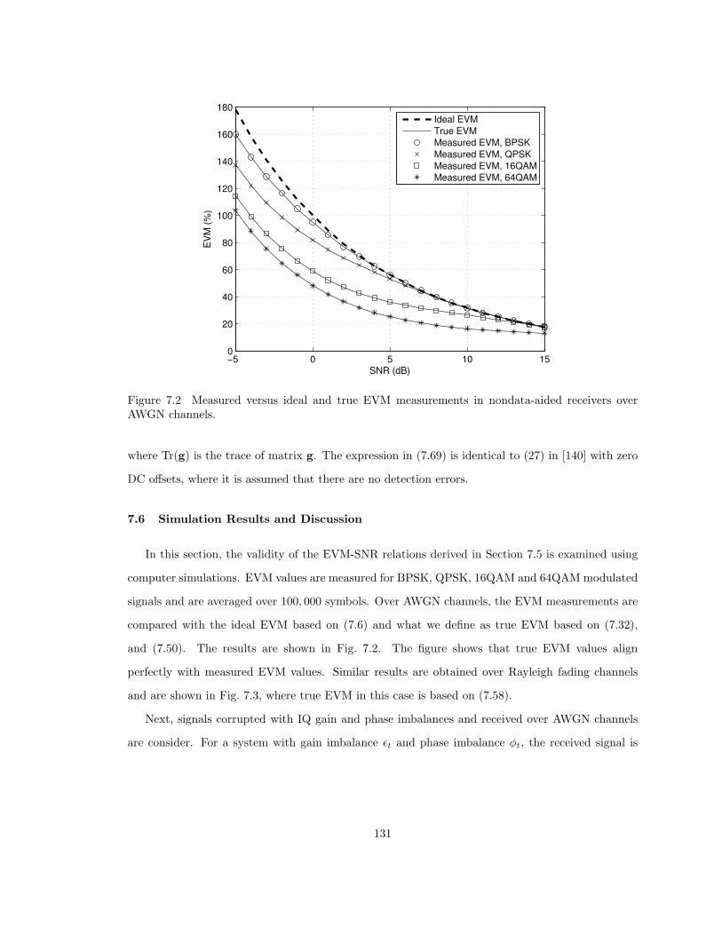
−5 0 5 10 150
20
40
60
80
100
120
140
160
180
SNR (dB)
EV
M (
%)
Ideal EVM
True EVM
Measured EVM, BPSK
Measured EVM, QPSK
Measured EVM, 16QAM
Measured EVM, 64QAM
Figure 7.2 Measured versus ideal and true EVM measurements in nondata-aided receivers overAWGN channels.
where Tr(g) is the trace of matrix g. The expression in (7.69) is identical to (27) in [140] with zero
DC offsets, where it is assumed that there are no detection errors.
7.6 Simulation Results and Discussion
In this section, the validity of the EVM-SNR relations derived in Section 7.5 is examined using
computer simulations. EVM values are measured for BPSK, QPSK, 16QAM and 64QAM modulated
signals and are averaged over 100, 000 symbols. Over AWGN channels, the EVM measurements are
compared with the ideal EVM based on (7.6) and what we define as true EVM based on (7.32),
and (7.50). The results are shown in Fig. 7.2. The figure shows that true EVM values align
perfectly with measured EVM values. Similar results are obtained over Rayleigh fading channels
and are shown in Fig. 7.3, where true EVM in this case is based on (7.58).
Next, signals corrupted with IQ gain and phase imbalances and received over AWGN channels
are consider. For a system with gain imbalance εt and phase imbalance φt, the received signal is
131
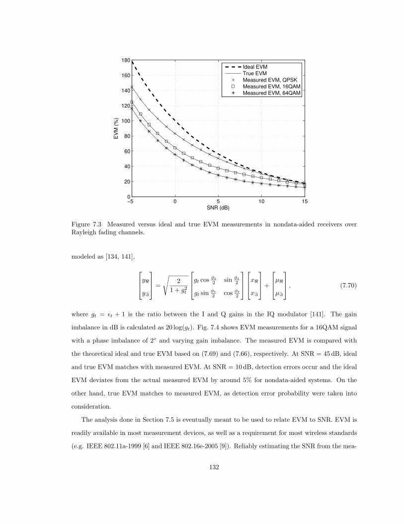
−5 0 5 10 150
20
40
60
80
100
120
140
160
180
SNR (dB)
EV
M (
%)
Ideal EVM
True EVM
Measured EVM, QPSK
Measured EVM, 16QAM
Measured EVM, 64QAM
Figure 7.3 Measured versus ideal and true EVM measurements in nondata-aided receivers overRayleigh fading channels.
modeled as [134, 141],
y<
y=
=
√2
1 + g2t
gt cos φt
2 sin φt
2
gt sin φt
2 cos φt
2
x<
x=
+
µ<
µ=
, (7.70)
where gt = εt + 1 is the ratio between the I and Q gains in the IQ modulator [141]. The gain
imbalance in dB is calculated as 20 log(gt). Fig. 7.4 shows EVM measurements for a 16QAM signal
with a phase imbalance of 2◦ and varying gain imbalance. The measured EVM is compared with
the theoretical ideal and true EVM based on (7.69) and (7.66), respectively. At SNR = 45 dB, ideal
and true EVM matches with measured EVM. At SNR = 10 dB, detection errors occur and the ideal
EVM deviates from the actual measured EVM by around 5% for nondata-aided systems. On the
other hand, true EVM matches to measured EVM, as detection error probability were taken into
consideration.
The analysis done in Section 7.5 is eventually meant to be used to relate EVM to SNR. EVM is
readily available in most measurement devices, as well as a requirement for most wireless standards
(e.g. IEEE 802.11a-1999 [6] and IEEE 802.16e-2005 [9]). Reliably estimating the SNR from the mea-
132
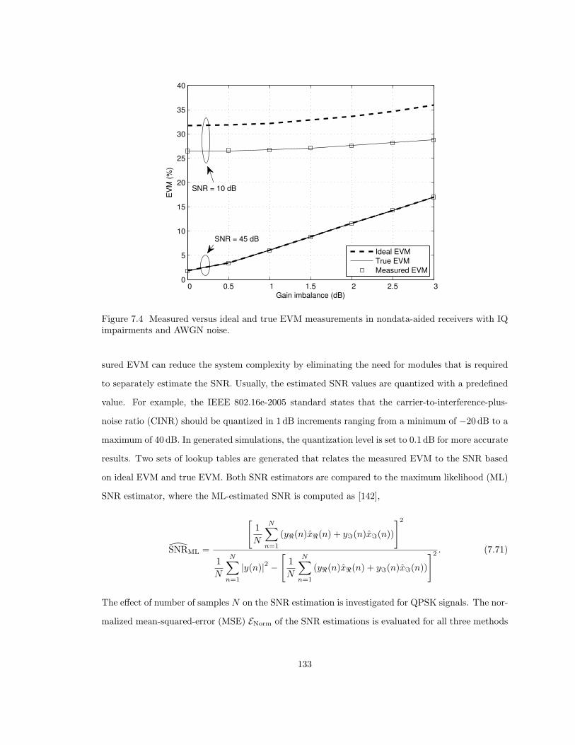
0 0.5 1 1.5 2 2.5 30
5
10
15
20
25
30
35
40
Gain imbalance (dB)
EV
M (
%)
Ideal EVM
True EVM
Measured EVM
SNR = 10 dB
SNR = 45 dB
Figure 7.4 Measured versus ideal and true EVM measurements in nondata-aided receivers with IQimpairments and AWGN noise.
sured EVM can reduce the system complexity by eliminating the need for modules that is required
to separately estimate the SNR. Usually, the estimated SNR values are quantized with a predefined
value. For example, the IEEE 802.16e-2005 standard states that the carrier-to-interference-plus-
noise ratio (CINR) should be quantized in 1 dB increments ranging from a minimum of −20 dB to a
maximum of 40 dB. In generated simulations, the quantization level is set to 0.1 dB for more accurate
results. Two sets of lookup tables are generated that relates the measured EVM to the SNR based
on ideal EVM and true EVM. Both SNR estimators are compared to the maximum likelihood (ML)
SNR estimator, where the ML-estimated SNR is computed as [142],
SNRML =
[1
N
N∑
n=1
(y<(n)x<(n) + y=(n)x=(n))
]2
1
N
N∑
n=1
|y(n)|2 −[
1
N
N∑
n=1
(y<(n)x<(n) + y=(n)x=(n))
]2 . (7.71)
The effect of number of samples N on the SNR estimation is investigated for QPSK signals. The nor-
malized mean-squared-error (MSE) ENorm of the SNR estimations is evaluated for all three methods
133
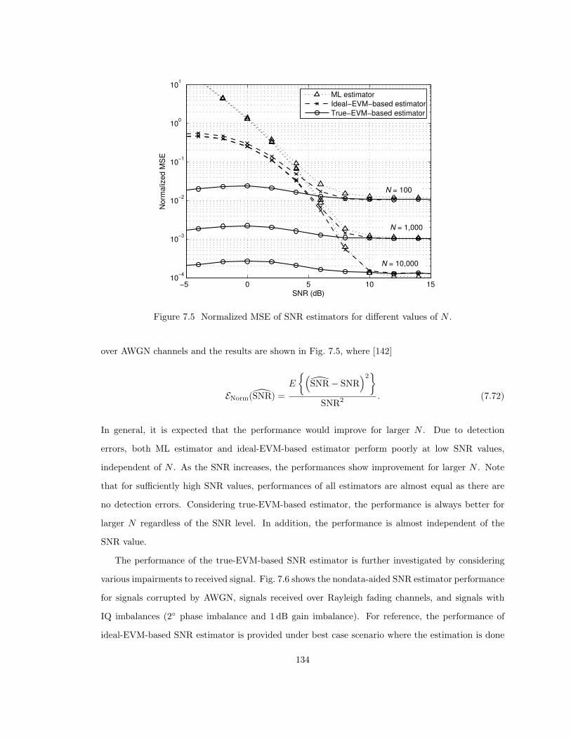
−5 0 5 10 1510
−4
10−3
10−2
10−1
100
101
SNR (dB)
Norm
aliz
ed M
SE
ML estimator
Ideal−EVM−based estimator
True−EVM−based estimator
N = 100
N = 10,000
N = 1,000
Figure 7.5 Normalized MSE of SNR estimators for different values of N .
over AWGN channels and the results are shown in Fig. 7.5, where [142]
ENorm(SNR) =
E
{(SNR − SNR
)2}
SNR2 . (7.72)
In general, it is expected that the performance would improve for larger N . Due to detection
errors, both ML estimator and ideal-EVM-based estimator perform poorly at low SNR values,
independent of N . As the SNR increases, the performances show improvement for larger N . Note
that for sufficiently high SNR values, performances of all estimators are almost equal as there are
no detection errors. Considering true-EVM-based estimator, the performance is always better for
larger N regardless of the SNR level. In addition, the performance is almost independent of the
SNR value.
The performance of the true-EVM-based SNR estimator is further investigated by considering
various impairments to received signal. Fig. 7.6 shows the nondata-aided SNR estimator performance
for signals corrupted by AWGN, signals received over Rayleigh fading channels, and signals with
IQ imbalances (2◦ phase imbalance and 1 dB gain imbalance). For reference, the performance of
ideal-EVM-based SNR estimator is provided under best case scenario where the estimation is done
134
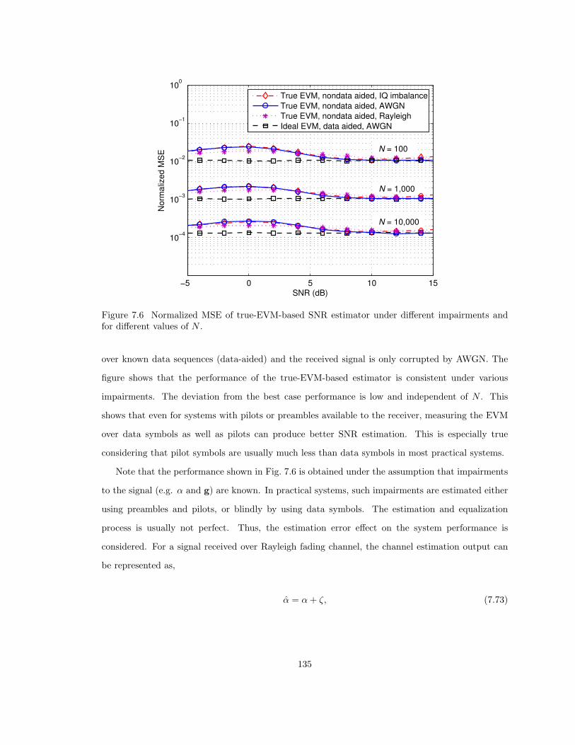
−5 0 5 10 15
10−4
10−3
10−2
10−1
100
SNR (dB)
No
rma
lize
d M
SE
True EVM, nondata aided, IQ imbalance
True EVM, nondata aided, AWGN
True EVM, nondata aided, Rayleigh
Ideal EVM, data aided, AWGN
N = 100
N = 1,000
N = 10,000
Figure 7.6 Normalized MSE of true-EVM-based SNR estimator under different impairments andfor different values of N .
over known data sequences (data-aided) and the received signal is only corrupted by AWGN. The
figure shows that the performance of the true-EVM-based estimator is consistent under various
impairments. The deviation from the best case performance is low and independent of N . This
shows that even for systems with pilots or preambles available to the receiver, measuring the EVM
over data symbols as well as pilots can produce better SNR estimation. This is especially true
considering that pilot symbols are usually much less than data symbols in most practical systems.
Note that the performance shown in Fig. 7.6 is obtained under the assumption that impairments
to the signal (e.g. α and g) are known. In practical systems, such impairments are estimated either
using preambles and pilots, or blindly by using data symbols. The estimation and equalization
process is usually not perfect. Thus, the estimation error effect on the system performance is
considered. For a signal received over Rayleigh fading channel, the channel estimation output can
be represented as,
α = α + ζ, (7.73)
135
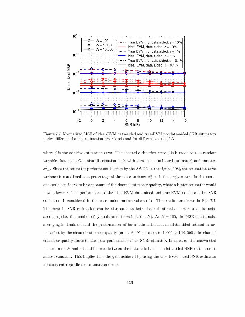
−2 0 2 4 6 8 10 12 14 16
10−4
10−3
10−2
10−1
100
SNR (dB)
No
rma
lize
d M
SE
N = 100
N = 1,000
N = 10,000
True EVM, nondata aided, ε = 10%
Ideal EVM, data aided, ε = 10%
True EVM, nondata aided, ε = 1%
Ideal EVM, data aided, ε = 1%
True EVM, nondata aided, ε = 0.1%
Ideal EVM, data aided, ε = 0.1%
Figure 7.7 Normalized MSE of ideal-EVM data-aided and true-EVM nondata-aided SNR estimatorsunder different channel estimation error levels and for different values of N .
where ζ is the additive estimation error. The channel estimation error ζ is is modeled as a random
variable that has a Gaussian distribution [140] with zero mean (unbiased estimator) and variance
σ2est. Since the estimator performance is affect by the AWGN in the signal [108], the estimation error
variance is considered as a percentage of the noise variance σ2n such that, σ2
est = εσ2n. In this sense,
one could consider ε to be a measure of the channel estimator quality, where a better estimator would
have a lower ε. The performance of the ideal EVM data-aided and true EVM nondata-aided SNR
estimators is considered in this case under various values of ε. The results are shown in Fig. 7.7.
The error in SNR estimation can be attributed to both channel estimation errors and the noise
averaging (i.e. the number of symbols used for estimation, N). At N = 100, the MSE due to noise
averaging is dominant and the performances of both data-aided and nondata-aided estimators are
not affect by the channel estimator quality (or ε). As N increases to 1, 000 and 10, 000 , the channel
estimator quality starts to affect the performance of the SNR estimator. In all cases, it is shown that
for the same N and ε the difference between the data-aided and nondata-aided SNR estimators is
almost constant. This implies that the gain achieved by using the true-EVM-based SNR estimator
is consistent regardless of estimation errors.
136
7.7 Conclusion
In this chapter, measured EVM is related to SNR for nondata-aided receivers, called true EVM.
True EVM is related to the SNR for QAM and PAM signals. The EVM-SNR relation is evaluated
for signals detected over AWGN channels, and Rayleigh fading channels; and for signals with IQ
impairments. The derived expressions are verified using computer simulations. The presented results
show that when considering nondata-aided receivers, using EVM-SNR relations derived for data-
aided receivers (or assuming high SNR) results in poor SNR estimation especially for high modulation
orders or low SNR values. On the other hand, using proposed true EVM expressions results in
accurate SNR estimation independent of modulation order and SNR value.
137
CHAPTER 8
CONCLUSION AND FUTURE WORK
In this dissertation, we considered the transceiver design for orthogonal frequency division mul-
tiplexing (OFDM) and orthogonal frequency division multiple access (OFDMA) advanced systems.
In Chapter 2, we introduced OFDM technology and discussed its advantages and disadvantages
when applied to future wireless systems. For the remainder of the dissertation, we focused on some
of the important challenges that face OFDM-based systems. Practical implementation aspects such
as computational complexity, power consumption, bit error rate (BER), and adjacent channel inter-
ference (ACI) are considered. Parts of the work presented in this dissertation have been accepted
for publication [20–27] and has been recognized by the wireless research community through cita-
tions [143–150]. The study we presented in [22] has been the second most accessed document on the
IEEE Xplore R© [151] for the month of June, 2008. Some of the specific contributions presented in
this dissertation are listed below.
8.1 Contributions
• Synchronization in OFDMA Uplink Systems
A novel algorithm for OFDMA initial ranging process based on the IEEE 802.16e-2005 stan-
dard is presented in Chapter 3. The proposed algorithm performs multiuser code detection
and timing offset estimation for ranging users. It was shown that the proposed algorithm
reduces the computational complexity by 80% to 96% depending on the number of users while
maintaining the standard deviation of the timing error under 5% of the guard interval. Simula-
tion results showed that the proposed algorithm can perform well with as high as 10 users per
ranging channel in a given uplink (UL) frame. Hence, the proposed algorithm can be highly
desirable for practical OFDMA-based base stations (BS).
138
• Spectrum Shaping for OFDM Systems
We proposed a new method, called adaptive symbol transition (AST), to suppress OFDM
sidelobes adaptively and allow the system to shape the transmitted signal spectrum. The
proposed AST method extends OFDM symbols and uses the extension to reduce ACI to other
users operating in the same band. Simulation results show that AST can achieve a significant
gain over conventional sidelobe suppression techniques while maintaining low increase in sym-
bol energy. Moreover, AST does not increase the signal peak-to-average-power ratio (PAPR)
and the performance is not sensitive to other system parameters such as the cyclic prefix (CP)
size.
• OFDMA Performance under Channel Estimation Errors
We derived the BER expressions for OFDM signals received over time-varying frequency-
selective channels with channel estimation errors. The results were used to obtain the optimum
tile dimensions (or optimum pilot insertion rate) in the time-frequency grid. Both analytical
and simulated results show that careful choice of the tile dimensions can significantly increase
the system throughput.
• OFDMA Channel Estimation with IQ Imbalances
When considering the UL signal in OFDMA-based zero-IF systems, imperfections of the IQ-
modulators causes multiuser interference (MUI). We designed a two-dimensional orthogonal
pilot pattern to be used for channel estimation and equalization in this case. Two low com-
plexity methods are proposed to equalize and detect IQ distorted signals using designed pilot
pattern. Proposed methods were shown to improve the system performance significantly over
conventional detection methods for signals suffering from multiple user IQ distortions.
• EVM-based SNR Estimation in Blind Receivers
We derived the error vector magnitude (EVM) to signal-to-noise ratio (SNR) relations for
signals detected over additive white Gaussian noise (AWGN) channels, and Rayleigh fading
channels; and for signals with IQ impairments. The presented results show that when consid-
ering blind receivers, using EVM-SNR relations derived for data-aided receivers (or assuming
high SNR) results in poor SNR estimation especially for high modulation orders or low SNR
values. On the other hand, using proposed true EVM expressions results in accurate SNR
estimation independent of modulation order and SNR value.
139
8.2 Final Remarks and Future Work
OFDM system offers a number of advantages for high data rate wireless systems, but suffers from
some drawbacks. Throughout the dissertation, we tried to address some of the important challenges
that face OFDM implementation in practical wireless systems. Meanwhile, there were other research
topics that we feel are closely related to our work and can be a possible extension to the studies
presented in this dissertation. A discussion of these topics is presented in this section.
• Noncoherent Detection in OFDMA Uplink Systems
For OFDMA system to maintain orthogonality and reduce multiuser interference (MUI), syn-
chronization between users should be maintained. The approach we proposed in Chapter 3 can
be used in primary networks, where the base station (BS) can mandate the transmission time
of each user. However, for secondary networks, such as femto cell, users cannot be synchronized
prior to transmission. In that case, there is a need for an algorithm to detect received signal
under MUI effects through interference detection and cancellation methods. As such, the de-
sign and implementation of OFDMA systems in femto cell represents an interesting research
topic.
• Low-Complexity Spectrum Shaping for OFDM Systems
The method we proposed in Chapter 4, as well as most other sidelobe suppression techniques
proposed in the literature, suffer from high computational complexity. However, spectrum
shaping in cognitive radio (CR) systems needs to be performed online with minimum delay as
to take advantage of available spectrum opportunities. Thus, there is a need for an efficient
yet low-complexity methods for OFDM spectrum shaping. We are currently working on sub-
optimal adaptive symbol transition (AST) algorithm that can shape the spectrum of OFDM
signals with reduced computational complexity.
• OFDMA Capacity under Various Impairments
We evaluated the performance of OFDMA systems over wireless selective channels and under
channel estimation errors as well as IQ imbalances in Chapters 5 and 6. There are three
directions in which this work can be extended. First, the performance of OFDMA systems
can be examined under a number of other practical impairments such as timing and frequency
offsets or sampling clock errors.
140
Second, since tiles in the OFDMA uplink belong to multiple users, we assumed the receiver
carries out the estimation and equalization on a tile-by-tile basis. A possible improvement to
the channel estimation can be attained if the system has the ability to detect and use pilots
that belong to the same user but over different tiles. To achieve this goal the system needs to
have prior knowledge, to some extend, of the user channel correlation over time and frequency.
Third, the optimum tile dimensions introduced in Chapter 5 were obtained for hard decision
receivers using channel capacity and upper bounds on convolutional codes. This work can
be extended to obtain the optimum tile dimensions for soft decision receivers. In this case,
we need to derive the probability distributions of received signal as function of the wireless
selective channel and the channel estimation errors for a given system model.
141
REFERENCES
[1] FCC Spectrum Policy Task Force, “FCC report of the spectrum efficiency working group,”Federal Communications Commission, Tech. Rep., Nov. 2002.
[2] J. Mitola and G. Q. Maguire Jr., “Cognitive radio: Making software radios more personal,”IEEE Personal Communications, vol. 6, no. 4, pp. 13–18, Aug. 1999.
[3] J. Mitola, “Cognitive radio,” Licentiate Thesis, Dept. of Teleinformatics, Royal Institute ofTechnology, Sep. 1999.
[4] S. Haykin, “Cognitive radio: brain-empowered wireless communications,” IEEE J. Select.Areas Commun., vol. 3, no. 2, pp. 201–220, Feb. 2005.
[5] “Broadband radio access networks (BRAN); HIPERLAN type 2; physical (PHY) layer,” ETSIStd. TS 101 475, 2001.
[6] “Supplement to IEEE standard for information technology telecommunications and informa-tion exchange between systems - local and metropolitan area networks - specific requirements.part 11: wireless LAN medium access control (MAC) and physical layer (PHY) specifications:high-speed physical layer in the 5 GHz band,” IEEE Std. 802.11a-1999, 1999.
[7] “Broadband mobile access communication system (HiSWANa),” ARIB Std. H14.11.27, 2002.
[8] “IEEE standard for local and metropolitan area networks part 16: Air interface for fixedbroadband wireless access systems,” IEEE Std. 802.16-2004 (Revision of IEEE Std. 802.16-2001), 2004.
[9] “IEEE standard for local and metropolitan area networks part 16: Air interface for fixed andmobile broadband wireless access systems amendment 2: Physical and medium access controllayers for combined fixed and mobile operation in licensed bands and corrigendum 1,” IEEEStd. 802.16e-2005 and IEEE Std. 802.16-2004/Cor 1-2005 (Amendment and Corrigendum toIEEE Std. 802.16-2004), 2006.
[10] “Asymmetric digital subscriber line (ADSL),” ANSI Std. T1.413, 1995.
[11] “Radio broadcasting systems; digital audio broadcasting (DAB) to mobile, portable and fixedreceivers,” ETSI Std. EN 300 401, 2001.
[12] “Digital video broadcasting (DVB); framing structure, channel coding and modulation fordigital terrestrial television,” ETSI Std. EN 300 744, 2001.
[13] “IEEE 802.15 WPAN high rate alternative PHY task group 3a (TG3a),”http://www.ieee802.org/15/pub/TG3a.html.
[14] E. Seidel, “Progress on LTE Advanced - the new 4G standard,” White Paper, Nomor Research,Jul. 2008.
[15] http://www.ist-winner.org.
142
[16] “IEEE 802.22 working group on wireless regional area networks.” [Online]. Available:http://www.ieee802.org/22/
[17] A. A. Abidi, “Direct-conversion radio transceivers for digital communications,” IEEE J. Solid-State Circuits, vol. 30, no. 12, pp. 1399–1410, 1995.
[18] B. Come, R. Ness, S. Donnay, L. Van der Perre, W. Eberle, P. Wambacq, M. Engels, andI. Bolsens, “Impact of front-end non-idealities on bit error rate performance of WLAN-OFDMtransceivers,” in Proc. IEEE Radio and Wireless Conf. (RAWCON), 2000, pp. 91–94.
[19] R. Liu, Y. Li, H. Chen, and Z. Wang, “EVM estimation by analyzing transmitter imperfectionsmathematically and graphically,” Springer Analog Integrated Circuits and Signal ProcessingJournal, vol. 48, no. 3, pp. 257–262, 2006.
[20] H. A. Mahmoud, T. Yucek, and H. Arslan, Cognitive Radio, Software Defined Radio, andAdaptive Wireless Systems. Springer, 2007, ch. OFDM for Cognitive Radio: Merits andChallenges.
[21] ——, “OFDM for cognitive radio: Merits and challenges,” accepted for publication in IEEEWireless Commun. Mag., 2009.
[22] H. A. Mahmoud, H. Arslan, and M. K. Ozdemir, “Initial ranging for WiMAX (802.16e)OFDMA,” in Proc. IEEE Mil. Commun. Conf. (MILCOM), 2006.
[23] ——, “An efficient ranging algorithm for WiMAX (802.16e) OFDMA,” Elsevier Comput. Com-mun. J., vol. 32, no. 1, pp. 159–168, Jan. 2009.
[24] H. A. Mahmoud and H. Arslan, “Sidelobe suppression in OFDM-based spectrum sharingsystems using adaptive symbol transition,” IEEE Commun. Lett., vol. 12, no. 2, pp. 133–135,Feb. 2008.
[25] ——, “Spectrum shaping of OFDM-based cognitive radio signals,” in Proc. IEEE Radio andWireless Sym. (RWS), Jan. 2008.
[26] H. A. Mahmoud, H. Arslan, M. K. Ozdemir, and F. E. Retnasothie, “IQ imbalance correctionfor OFDMA uplink systems,” accepted for publication in Proc. IEEE Int. Conf. Commun.(ICC), Jun. 2009.
[27] H. A. Mahmoud and H. Arslan, “Error vector magnitude to snr conversion for nondata aidedreceivers,” accepted for publication in IEEE Trans. Wireless Commun., 2009.
[28] P. Robertson and S. Kaiser, “The effect of Doppler spreads in OFDM(A) mobile radio sys-tems,” in Proc. IEEE Veh. Technol. Conf. (VTC), vol. 1, Sep. 1999, pp. 329–333.
[29] D. T. Harvatin and R. E. Ziemer, “Orthogonal frequency division multiplexing performancein delay and doppler spread channels,” in Proc. IEEE Veh. Technol. Conf. (VTC), vol. 3, May1997.
[30] S. Hara and R. Prasad, “Overview of multicarrier CDMA,” IEEE Commun. Mag., vol. 35,no. 12, pp. 126–133, Dec. 1997.
[31] H. Yaghoobi, “Scalable OFDMA physical layer in IEEE 802.16 WirelessMAN,” Intel Technol-ogy Journal, vol. 8, no. 3, pp. 201–212, Aug. 2004.
[32] T. Yucek, “Channel, spectrum and waveform awareness in OFDM-based Cognitive Radiosystems,” Ph.D. dissertation, University of South Florida, Jul. 2007.
143
[33] M. Wylie-Green, “Dynamic spectrum sensing by multiband OFDM radio for interference mit-igation,” in Proc. IEEE Int. Sym. on New Frontiers in Dynamic Spectr. Access Netw. (DyS-PAN), 2005, pp. 619–625.
[34] T. Weiss, J. Hillenbrand, and F. Jondral, “A diversity approach for the detection of idlespectral resources in spectrum pooling systems,” in Proc. of the 48th Int. Scientific Colloquium,Ilmenau, Germany, Sep. 2003.
[35] J. Hillenbrand, T. A. Weiss, and F. K. Jondral, “Calculation of detection and false alarmprobabilities in spectrum pooling systems,” IEEE Commun. Lett., vol. 9, no. 4, pp. 349–351,2005.
[36] T. Yucek and H. Arslan, “Spectrum characterization for opportunistic cognitive radio sys-tems,” in Proc. IEEE Mil. Commun. Conf. (MILCOM), 2006, pp. 1–6.
[37] H. Arslan and T. Yucek, Adaptation Techniques in Wireless Multimedia Networks. NovaScience Publishers, 2006, ch. Adaptation of Wireless Mobile Multi-carrier Systems.
[38] T. Keller and L. Hanzo, “Adaptive modulation techniques for duplex OFDM transmission,”IEEE Trans. Veh. Technol., vol. 49, no. 5, pp. 1893–1906, Sep. 2000.
[39] C. Y. Wong, R. S. Cheng, K. B. Lataief, and R. D. Murch, “Multiuser OFDM with adaptivesubcarrier, bit, and power allocation,” IEEE J. Sel. Areas Commun., vol. 17, no. 10, pp.1747–1758, Oct. 1999.
[40] S. W. Lei and V. K. N. Lau, “Adaptive interleaving for OFDM in TDD systems,” IEE Proc.Commun., vol. 148, no. 2, pp. 77–80, 2001.
[41] A. Dowler, A. Doufexi, and A. Nix, “Performance evaluation of channel estimation techniquesfor a mobile fourth generation wide area OFDM system,” in Proc. IEEE Veh. Technol. Conf.(VTC), vol. 4, 2002.
[42] S. Haykin and M. Moher, Modern Wireless Communications. New York, NY: Prentice-Hall,2004.
[43] Y. Li and N. Sollenberger, “Interference suppression in OFDM systems using adaptive antennaarrays,” in Proc. IEEE Global Telecommun. Conf. (GLOBECOM), vol. 1, Nov. 1998, pp. 213–218.
[44] Institute of Electrical and Electronics Engineers, “IEEE standard computer dictionary: Acompilation of IEEE standard computer glossaries,” New York, NY, 1990.
[45] SDR Forum, “Software Defined Radio Technology for Public Safety,” SDR Forum, Apr. 14,2006, approved Document SDRF–06–A–0001–V0.00.
[46] “IEEE standard for information technology- telecommunications and information exchangebetween systems- local and metropolitan area networks- specific requirements part 11: wirelessLAN medium access control (MAC) and physical layer (PHY) specifications,” IEEE Std.802.11g-2003 (Amendment to IEEE Std. 802.11, 1999 Edn. (Reaff 2003) as amended by IEEEStds 802.11a-1999, 802.11b-1999, 802.11b-1999/Cor 1-2001, and 802.11d-2001), 2003.
[47] A. Batra, J. Balakrishnan, G. Aiello, J. Foerster, and A. Dabak, “Design of a multibandOFDM system for realistic UWB channel environments,” IEEE Trans. Microw. Theory Tech.,vol. 52, no. 9, pp. 2123–2138, 2004.
144
[48] V. S. Somayazulu, J. R. Foerster, and S. Roy, “Design challenges for very high data rateUWB systems,” in Proc. IEEE Asilomar Conf. on Signals, Systems and Computers, 2002, pp.717–721.
[49] D. M. W. Leenaerts, “Transceiver design for multiband OFDM UWB,” EURASIP J. on Wire-less Commun. and Netw., vol. 2006, no. 2, pp. 25–25, 2006.
[50] H. Zheng and H. C. Luong, “A 1.5 V 3.1 GHz8 GHz CMOS synthesizer for 9-band MB-OFDMUWB transceivers,” IEEE J. Solid-State Circuits, vol. 42, no. 6, pp. 1250–1260, Jun. 2007.
[51] B. Razavi, T. Aytur, C. Lam, F.-R. Yang, R.-H. Yan, H.-C. Kang, C.-C. Hsu, and C.-C. Lee,“Multiband UWB transceivers,” in Proc. IEEE Custom Integr. Circuits Conf. (CICC), Sep.2005, pp. 141–148.
[52] J. Lee and D. Chiu, “A 7-band 3–8 GHz frequency synthesizer with 1 ns band-switching timein 0.18 m CMOS technology,” in Proc. IEEE Custom Integr. Circuits Conf. (CICC), 2005, pp.204–205.
[53] A. Ismail and A. Abidi, “A 3.1 to 8.2 GHz direct conversion receiver for MB-OFDM UWBcommunications,” in Proc. IEEE Int. Solid State Circuits Conf. (ISSCC), vol. 1, Feb. 2005,pp. 208–593.
[54] R. Rajbanshi, A. M. Wyglinski, , and G. J. Minden, “An efficient implementation of NC-OFDM transceivers for cognitive radios,” in Proc. IEEE Int. Conf. on Cognitive Radio Ori-ented Wireless Netw. and Commun. (CROWNCOM), Jun. 2006.
[55] H. Celebi and H. Arslan, “Cognitive positioning systems,” IEEE Trans. Wireless Commun.,vol. 6, no. 12, pp. 4475–4483, 2007.
[56] ——, “Utilization of location information in cognitive wireless networks,” IEEE Wireless Com-mun. Mag., vol. 14, no. 4, pp. 6–13, 2007.
[57] H. Celebi, “Location awareness in Cognitive Radio networks,” Ph.D. dissertation, Universityof South Florida, Aug. 2008.
[58] D. E. Breen Jr, “Characterization of multi-carrier locator performance,” Master’s thesis,Worcester Polytechnic Institute, May 2004.
[59] A. M. Wyglinski, “Effects of bit allocation on non-contiguous multicarrier-based cognitiveradio transceivers,” in Proc. IEEE Veh. Technol. Conf. (VTC), Sep. 2006.
[60] T. Weiss and F. K. Jondral, “Spectrum pooling: an innovative strategy for the enhancementof spectrum efficiency,” IEEE Commun. Mag., vol. 42, no. 3, pp. 8–14, Mar. 2004.
[61] T. Weiss, A. Krohn, F. Capar, I. Martoyo, and F. Jondral, “Synchronization algorithms andpreamble concepts for spectrum pooling systems,” in IST Mobile and Wireless Telecommun.Summit, Jun. 2003.
[62] C. Muschallik, “Improving an OFDM reception using an adaptive Nyquist windowing,” IEEETrans. Consum. Electron., vol. 42, no. 3, pp. 259–269, Aug. 1996.
[63] S. H. Muller-Weinfurtner, “Optimum Nyquist windowing in OFDM receivers,” IEEE Trans.Commun., vol. 49, no. 3, pp. 417–420, Mar. 2001.
[64] T. Weiss, J. Hillenbrand, A. Krohn, and F. K. Jondral, “Mutual interference in OFDM-basedspectrum pooling systems,” in Proc. IEEE Veh. Technol. Conf. (VTC), vol. 4, May 2004, pp.1873–1877.
145
[65] H. Yamaguchi, “Active interference cancellation technique for MB-OFDM cognitive radio,” inProc. IEEE European Microwave Conf., vol. 2, Oct. 2004, pp. 1105–1108.
[66] S. Brandes, I. Cosovic, and M. Schnell, “Sidelobe suppression in OFDM systems by insertionof cancellation carriers,” in Proc. IEEE Veh. Technol. Conf. (VTC), vol. 1, Sep. 2005, pp.152–156.
[67] ——, “Reduction of out-of-band radiation in OFDM systems by insertion of cancellation car-riers,” IEEE Commun. Lett., vol. 10, no. 6, pp. 420–422, Jun. 2006.
[68] S. Pagadarai, R. Rajbanshi, A. M. Wyglinski, and G. J. Minden, “Sidelobe suppression forOFDM-based cognitive radios using constellation expansion,” in Proc. IEEE Wireless Com-mun. and Netw. Conf. (WCNC), Apr. 2008, pp. 888–893.
[69] “IEEE standard for local and metropolitan area networks — part 16: Air interface for fixedbroadband wireless access systems— amendment 2: Medium access control modifications andadditional physical layer specifications for 2-11 GHz,” IEEE Std. 802.16a-2003 (Amendmentto IEEE Std. 802.16-2001), 2003.
[70] T. S. Rappaport, Smart Antennas: Adaptive Arrays, Algorithms, and Wireless Position Loca-tion. IEEE, 1998.
[71] O. Hoshuyama, A. Sugiyama, and A. Hirano, “A robust adaptive beamformer for microphonearrays with a blocking matrix using constrained adaptive filters,” IEEE Trans. Signal Process.,vol. 47, no. 10, pp. 2677–2684, 1999.
[72] S. Brandes, I. Cosovic, and M. Schnell, “Reduction of out-of-band radiation in OFDM basedoverlay systems,” in Proc. IEEE Int. Sym. on New Frontiers in Dynamic Spectr. Access Netw.(DySPAN), Nov. 2005, pp. 662–665.
[73] I. Cosovic, S. Brandes, and M. Schnell, “A technique for sidelobe suppression in OFDM sys-tems,” in Proc. IEEE Global Telecommun. Conf. (GLOBECOM), vol. 1, Nov. 2005, pp. 204–208.
[74] ——, “Subcarrier weighting: a method for sidelobe suppression in OFDM systems,” IEEECommun. Lett., vol. 10, no. 6, pp. 444–446, Jun. 2006.
[75] I. Cosovic and T. Mazzoni, “Suppression of sidelobes in OFDM systems by multiple-choicesequences,” European Trans. Telecommun., vol. 17, no. 6, pp. 623–630, 2006.
[76] G. Dong, H. Chen, M. Yang, and J. Dai, “Dynamic frequency selection (DFS) in IEEE802.16eOFDM system working at unlicensed bands,” in Proc. IEEE Int. Conf. on Adv. Commun.Tech. (ICACT), vol. 2, Feb. 2007.
[77] T. C. H. Alen, A. S. Madhukumar, and F. Chin, “Capacity enhancement of a multi-userOFDM system using dynamic frequency allocation,” IEEE Trans. Broadcast., vol. 49, no. 4,pp. 344–353, Dec. 2003.
[78] “Supplement to IEEE standard for information technology- telecommunications and informa-tion exchange between systems- local and metropolitan area networks- specific requirements-part II: Wireless LAN medium access control (MAC) and physical layer (PHY) specifications:Higher-speed physical layer extension in the 2.4 GHz band,” IEEE Std. 802.11b-1999, 2000.
[79] http://www.wi-fi.org.
[80] T. M. Schmidl and D. C. Cox, “Robust frequency and timing synchronization for OFDM,”IEEE Trans. Commun., vol. 45, no. 12, pp. 1613–1621, Dec. 1997.
146
[81] J. J. van de Beek, P. O. Borjesson, M.-L. Boucheret, D. Landstrom, J. Arenas, P. Odling,C. Ostberg, M. Wahlqvist, and S. K. Wilson, “A time and frequency synchronization schemefor multiuser OFDM,” IEEE J. Select. Areas Commun., vol. 17, no. 11, pp. 1900–1914, Nov.1999.
[82] M. Morelli, “Timing and frequency synchronization for the uplink of an OFDMA system,”IEEE Trans. Commun., vol. 52, no. 2, pp. 296–306, Feb. 2004.
[83] X. Fu and H. Minn, “Initial uplink synchronization and power control (ranging process) forOFDMA systems,” in Proc. IEEE Global Telecommun. Conf. (GLOBECOM), vol. 6, Nov. 29-Dec. 3, 2004, pp. 3999–4003.
[84] J. Krinock, M. Singh, M. Paff, V. Tien, A. Lonkar, L. Fung, and C.-C. Lee, “Comments onOFDMA ranging scheme described in IEEE 802.16ab-01/01r1,” IEEE 802.16abc-01/24, Aug.2001.
[85] J. J. van de Beek, M. Sandell, and P. O. Borjesson, “ML estimation of time and frequencyoffset in OFDM systems,” IEEE Trans. Signal Process., vol. 45, no. 7, pp. 1800–1805, 1997.
[86] I. L. standards committee, “Air interface for fixed broadband wireless access systems,” July2001.
[87] D. H. Lee, “OFDMA uplink ranging for IEEE 802.16e using modified generalized chirp-likepolyphase sequences,” in Proc. IEEE and IFIP Int. Conf. in Central Asia on Internet, Sep.2005.
[88] H. Minn and X. Fu, “A new ranging method for OFDMA systems,” in Proc. IEEE GlobalTelecommun. Conf. (GLOBECOM), vol. 3, Nov. 28- Dec. 2, 2005.
[89] J. G. Proakis, Digital Communications, 4th ed. McGraw-Hill, 2001.
[90] WiMAX Forum, “WiMAX system evaluation methodology,” Sep. 2007.
[91] Recommendation ITU-R M.1225, “Guidelines for evaluation of radio transmission technologiesfor IMT-2000,” Int. Telecommun. Union (ITU), 1997.
[92] D. Cabric, S. M. Mishra, and R. W. Brodersen, “Implementation issues in spectrum sensing forcognitive radios,” in Proc. IEEE Asilomar Conf. on Signals, Systems and Computers, vol. 1,Nov. 2004, pp. 772–776.
[93] J. Heiskala and J. Terry, OFDM Wireless LANs: A Theoretical and Practical Guide. Samspublishing, 2002, ch. 2.
[94] W. Gander, “Least squares with a quadratic constraint,” Numerische Mathematik, vol. 36,no. 3, pp. 291–307, 1980.
[95] J. Bonnet and G. Auer, “Chunk-based channel estimation for uplink OFDM,” in Proc. IEEEVeh. Technol. Conf. (VTC), vol. 4, May 2006, pp. 1555–1559.
[96] Y. Ma and R. Tafazolli, “Channel estimation for OFDMA uplink: a hybrid of linear and BEMinterpolation approach,” IEEE Trans. Signal Process., vol. 55, no. 4, pp. 1568–1573, Apr.2007.
[97] H. Liu, Y. Ma, and R. Tafazolli, “Optimum pilot placement for chunk-based OFDMA uplink:Single chunk scenario,” in Proc. IEEE Veh. Technol. Conf. (VTC), Oct. 2007, pp. 2194–2198.
[98] ——, “Optimum pilot placement for chunk-based OFDMA uplink: Time direction scenario,”in Proc. IEEE Veh. Technol. Conf. (VTC), May 2008, pp. 2547–2551.
147
[99] P. Hoeher, S. Kaiser, and P. Robertson, “Two-dimensional pilot-symbol-aided channel esti-mation by Wiener filtering,” Proc. IEEE Int. Conf. on Acoust., Speech, and Signal Process.(ICASSP), vol. 3, pp. 1845–1848, Apr. 1997.
[100] P. Tan and N. C. Beaulieu, “Effect of channel estimation error on bit error probability inOFDM systems over rayleigh and ricean fading channels,” IEEE Trans. Commun., vol. 56,no. 4, pp. 675–685, Apr. 2008.
[101] Y. Li, L. J. Cimini, and N. R. Sollenberger, “Robust channel estimation for OFDM systemswith rapid dispersive fading channels,” IEEE Trans. Commun., vol. 46, no. 7, pp. 902–915,Jul. 1998.
[102] W. C. Jakes, Microwave mobile communications. Wiley, New York, 1974.
[103] Y.-S. Choi, P. J. Voltz, and F. A. Cassara, “On channel estimation and detection for multi-carrier signals in fast and selective rayleigh fading channels,” IEEE Trans. Commun., vol. 49,no. 8, pp. 1375–1387, Aug. 2001.
[104] M. Russell and G. L. Stuber, “Interchannel interference analysis of OFDM in a mobile envi-ronment,” in Proc. IEEE Veh. Technol. Conf. (VTC), vol. 2, Jul. 1995, pp. 820–824.
[105] Y. Li and L. J. Cimini, “Bounds on the interchannel interference of OFDM in time-varyingimpairments,” IEEE Trans. Commun., vol. 49, no. 3, pp. 401–404, Mar. 2001.
[106] X. Tang, M.-S. Alouini, and A. J. Goldsmith, “Effect of channel estimation error on M-QAMBER performance in Rayleigh fading,” IEEE Trans. Commun., vol. 47, no. 12, pp. 1856–1864,Dec. 1999.
[107] I. Gaspard, “Impact of the channel estimation onto the BER-performance of PSAM-OFDMsystems in mobile radio channels,” in Proc. IEEE Veh. Technol. Conf. (VTC), vol. 1, May2001, pp. 673–677.
[108] H. Cheon and D. Hong, “Effect of channel estimation error in OFDM-based WLAN,” IEEECommun. Lett., vol. 6, no. 5, pp. 190–192, 2002.
[109] M.-X. Chang and Y. T. Su, “Performance analysis of equalized OFDM systems in Rayleighfading,” IEEE Trans. Wireless Commun., vol. 1, no. 4, pp. 721–732, Oct. 2002.
[110] J. Chen, Y. Tang, S. Li, and Y. Li, “Effect of channel estimation error onto the BER per-formance of PSAM-OFDM in Rayleigh fading,” in Proc. IEEE Veh. Technol. Conf. (VTC),vol. 4, Oct. 2003, pp. 2444–2448.
[111] L. Cao and N. C. Beaulieu, “Exact error-rate analysis of diversity 16-QAM with channelestimation error,” IEEE Trans. Commun., vol. 52, no. 6, pp. 1019–1029, Jun. 2004.
[112] M. Al-Gharabally and P. Das, “On the performance of OFDM systems in time varying channelswith channel estimation error,” Proc. IEEE Int. Conf. Commun. (ICC), vol. 11, pp. 5180–5185,Jun. 2006.
[113] P. O. Borjesson and C.-E. W. Sundberg, “Simple approximations of the error function Q(x)for communications applications,” IEEE Trans. Commun., vol. 27, no. 3, pp. 639–643, Mar.1979.
[114] M. M. Wang, W. Xiao, and T. Brown, “Soft decision metric generation for QAM with channelestimation error,” IEEE Trans. Commun., vol. 50, no. 7, pp. 1058–1061, 2002.
148
[115] W. Xiao, “Optimal detection of M-QAM signal with channel estimation error,” Proc. IEEEInt. Conf. Commun. (ICC), vol. 5, pp. 3251–3255, May 2003.
[116] C. E. Shannon, “A mathematical theory of communication,” Bell Syst. Tech. J., vol. 27, no. 3,pp. 379–423, Jul. 1948.
[117] K. Larsen, “Short convolutional codes with maximal free distance for rates 1/2, 1/3, and 1/4,”IEEE Trans. Inf. Theory, vol. 19, no. 3, pp. 371–372, May 1973.
[118] P. Frenger, P. Orten, and T. Ottosson, “Convolutional codes with optimum distance spec-trum,” IEEE Commun. Lett., vol. 3, no. 11, pp. 317–319, Nov. 1999.
[119] A. R. Wright and P. A. Naylor, “I/Q mismatch compensation in zero-IF OFDM receiverswith application to DAB,” in Proc. IEEE Int. Conf. on Acoust., Speech, and Signal Process.(ICASSP), vol. 2, 2003.
[120] A. Tarighat and A. H. Sayed, “On the baseband compensation of IQ imbalances in OFDMsystems,” in Proc. IEEE Int. Conf. on Acoust., Speech, and Signal Process. (ICASSP), vol. 4,2004.
[121] J. Tubbax, B. Come, L. Van der Perre, L. Deneire, S. Donnay, and M. Engels, “Compensationof IQ imbalance in OFDM systems,” in Proc. IEEE Int. Conf. Commun. (ICC), vol. 5, 2003.
[122] H. Shafiee and S. Fouladifard, “Calibration of IQ imbalance in OFDM transceivers,” in Proc.IEEE Int. Conf. Commun. (ICC), vol. 3, 2003.
[123] J. Lin and E. Tsui, “Joint adaptive transmitter/receiver IQ imbalance correction for OFDMsystems,” in Proc. IEEE Int. Sym. on Pers., Indoor and Mobile Radio Commun. (PIMRC),vol. 2, 2004.
[124] A. Tarighat and A. H. Sayed, “OFDM systems with both transmitter and receiver IQ imbal-ances,” in Proc. IEEE Workshop on Signal Process. Adv. in Wireless Commun. (SPAWC),2005, pp. 735–739.
[125] T. C. W. Schenk, P. F. M. Smulders, and E. R. Fledderus, “Estimation and compensation ofTx and Rx IQ imbalance in OFDM-based MIMO systems,” in Proc. IEEE Radio and WirelessSym. (RWS), 2006, pp. 215–218.
[126] M. Valkama, Y. Zou, and M. Renfors, “On I/Q imbalance effects in MIMO space-time codedtransmission systems,” in Proc. IEEE Radio and Wireless Sym. (RWS), 2006, pp. 223–226.
[127] Y. Jin, J. Kwon, Y. Lee, D. Lee, and J. Ahn, “Obtained diversity gain in OFDM systemsunder the influence of IQ imbalance,” IEICE Trans. on Commun., vol. 91, no. 3, p. 814, 2008.
[128] L. Giugno, V. Lottici, and M. Luise, “Low-complexity gain and phase I/Q mismatch compen-sation using orthogonal pilot sequences,” in European Signal Process. Conf. (EUSIPCO), Sep.2006.
[129] R. Chrabieh and S. Soliman, “IQ imbalance mitigation via unbiased training sequences,” inProc. IEEE Global Telecommun. Conf. (GLOBECOM), Nov. 2007, pp. 4280–4285.
[130] A. Haider and A. Chatterjee, “Low-cost alternate EVM test for wireless receiver systems,” inProc. IEEE VLSI Test Sym., May 2005, pp. 255–260.
[131] R. Hassun, M. Flaherty, R. Matreci, and M. Taylor, “Effective evaluation of link quality usingerror vector magnitude techniques,” in Proc. IEEE Wireless Commun. Conf., Aug. 1997, pp.89–94.
149
[132] T. Nakagawa and K. Araki, “Effect of phase noise on RF communication signals,” in Proc.IEEE Veh. Technol. Conf. (VTC), vol. 2, Sep. 2000.
[133] M. Helfenstein, E. Baykal, K. Muller, A. Lampe, P. Semicond, and S. Zurich, “Error vectormagnitude (EVM) measurements for GSM/EDGE applications revised under production con-ditions,” in Proc. IEEE Int. Sym. on Circuits and Syst. (ISCAS), May 2005, pp. 5003–5006.
[134] A. Georgiadis, “Gain, phase imbalance, and phase noise effects on error vector magnitude,”IEEE Trans. Veh. Technol., vol. 53, no. 2, pp. 443–449, 2004.
[135] K. M. Gharaibeh, K. G. Gard, and M. B. Steer, “Accurate Estimation of Digital Communica-tion System Metrics – SNR, EVM and ρ in a Nonlinear Amplifier Environment,” IEEE Trans.Commun., pp. 734–739, Sep. 2005.
[136] R. A. Shafik, M. S. Rahman, A. R. Islam, and N. S. Ashraf, “On the Error Vector Magnitudeas a Performance Metric and Comparative Analysis,” International Conference on EmergingTechnologies (ICET), pp. 27–31, 2006.
[137] S. Forestier, P. Bouysse, R. Quere, A. Mallet, J. M. Nebus, and L. Lapierre, “Joint Optimiza-tion of the Power-Added Efficiency and the Error-Vector Measurement of 20-GHz pHEMT Am-plifier Through a New Dynamic Bias-Control Method,” IEEE Trans. Microw. Theory Tech.,vol. 52, no. 4, pp. 1132–1141, 2004.
[138] F. L. Lin and H. R. Chuang, “EVM and BER Simulation of an NADC-TDMA RadiophoneInfluenced by the Operator’s Body in Urban Mobile Environments,” Wireless Personal Com-munications, vol. 17, no. 1, pp. 135–147, 2001.
[139] N. L. Johnson and S. Kotz, Distributions in statistics: Continuous univariate distributions.John Wiley & Sons, 1970, vol. 1.
[140] M. Al-Gharabally and P. Das, “On the performance of OFDM systems in time varying channelswith channel estimation error,” in Proc. IEEE Int. Conf. Commun. (ICC), vol. 11, Jun. 2006,pp. 5180–5185.
[141] J. K. Cavers and M. W. Liao, “Adaptive compensation for imbalance and offset losses in directconversion transceivers,” IEEE Trans. Veh. Technol., vol. 42, no. 4, pp. 581–588, Nov. 1993.
[142] D. R. Pauluzzi and N. C. Beaulieu, “A comparison of SNR estimation techniques for theAWGN channel,” IEEE Trans. Commun., vol. 48, no. 10, pp. 1681–1691, Oct 2000.
[143] S. Soundararajan and P. Agrawal, “A scheduling algorithm for IEEE 802.16 and IEEE 802.11hybrid networks,” in Proc. IEEE Int. Conf. Broadband Commun., Netw. and Sys. (BROAD-NETS), 2007, pp. 320–322.
[144] D. H. Lee and H. Morikawa, “Non-synchronized random access process of single carrier FDMAsystem,” in Technical report of IEICE Radio Commun. Sys. (RCS), vol. 107, no. 147, 2007,pp. 137–142.
[145] ——, “Analysis on random access process of single carrier FDMA system,” in Proc. ICST Int.Conf. on Wireless Internet (WICON), 2007, pp. 1–9.
[146] J. Zeng and H. Minn, “A novel OFDMA ranging method exploiting multiuser diversity,” inProc. IEEE Global Telecommun. Conf. (GLOBECOM), Nov. 2007, pp. 1498–1502.
[147] ——, “Diversity exploiting MIMO-OFDMA ranging,” in Proc. IEEE Int. Conf. Information,Commun. and Signal Process. (ICICS), Dec. 2007, pp. 1–5.
150
[148] ——, “An investigation into initial ranging method for mobile OFDMA systems,” in Proc.IEEE Sarnoff Symposium, Apr. 2008, pp. 1–5.
[149] L. Sanguinetti, M. Morelli, and H. V. Poor, “An ESPRIT-based approach for initial rangingin OFDMA systems,” in Proc. IEEE Workshop on Signal Process. Adv. in Wireless Commun.(SPAWC), Jul. 2008.
[150] G. Bansal, M. J. Hossain, and V. K. Bhargava, “Optimal and suboptimal power allocationschemes for OFDM-based cognitive radio systems,” IEEE Trans. Wireless Commun., vol. 7,no. 11, pp. 4710–4718, Nov. 2008.
[151] http://ieeexplore.ieee.org.
151

APPENDICES
152
Appendix A
From (3.7), the expected value of Eg is,
E [Eg] = E
[L +
L−1∑
n=0
W 2<(m) +
L−1∑
n=0
W 2=(m) + 2
L−1∑
n=0
c(k)p (m) cos [φm(τk)]W<(m)
+ 2
L−1∑
n=0
c(k)p (m) sin [φm(τk)]W=(m)
]. (A.1)
Note that,
E[c(k)p (m)
]= 0, (A.2)
and,
E [W<(m)] = E [W=(m)] = 0. (A.3)
Since m values are randomly chosen between 0 and Nt − 1, φm(τk) can be approximated as a
uniformly-distributed random variable between π and −π. Thus,
E [cos [φm(τk)]] = E [sin [φm(τk)]] = 0. (A.4)
Therefore the expected value of the last two terms in (A.1) goes to zero for large values of L.
Then,
E [Eg] =L + E
[L−1∑
n=0
W 2<(m)
]+ E
[L−1∑
n=0
W 2=(m)
]
=L + LN0. (A.5)
Next, we calculate E[E2
g
]from (3.7). Note that,
E
(
L−1∑
n=0
W 2<(m)
)2 =
1
2LN2
0 +1
4L2N2
0 , (A.6)
153

Appendix A (Continued)
E
(
2L−1∑
n=0
c(k)p (m) cos [φm(τk)]W<(m)
)2 = LN0, (A.7)
E
[(L−1∑
n=0
W 2<(m)
)(L−1∑
n=0
W 2=(m)
)]=
1
2L2N2
0 . (A.8)
Then,
E[E2
g
]= L2 + LN2
0 + L2N20 + 2LN0 + 2L2N0. (A.9)
154
Appendix B
From (3.10),
Er(u) =L−1∑
n=0
{K−1∑
k=0
c(k)p (m) cos [φm(τk − u)]
}2
+L−1∑
n=0
W 2<(m)
+
L−1∑
n=0
[2W<(m) ·
K−1∑
k=0
c(k)p (m) cos [φm(τk − u)]
]
=
L−1∑
n=0
K−1∑
k=0
cos2 [φm(τk − u)]
+
L−1∑
n=0
K−1∑
k=0
K−1∑
v=0
v 6=k
{c(k)p (m)c(v)
p (m) cos [φm(τk − u)] cos [φm(τv − u)]
}
+L−1∑
n=0
W 2<(m) +
L−1∑
n=0
{2W<(m) cos [φm(u)]
K−1∑
k=0
c(k)p (m) cos [φm(τk − u)]
}. (B.1)
The expected value of the second and last terms in (B.1) is zero. Therefore,
E [Er(u)] =E
[L−1∑
n=0
K−1∑
k=0
cos2 [φm(τk − u)]
]+
E
[L−1∑
n=0
W 2<(m)
]. (B.2)
E [Er(u)] =
12LK + 1
2L + 12LN0 , for u = τk for
only one value of k.
12LK + 1
2LN0 , for u 6= τk for
all values of k.
(B.3)
The assumption that u = τk for only one value of k implies that in the same symbol and for a give
timing offset u, only one code exist.
155

Appendix C
The probability density function (PDF) of a random variable V that has a doubly-truncated
normal distribution is [139],
f(v) =1
σ
φ
(v − µ
σ
)
Φ
(B − µ
σ
)− Φ
(A − µ
σ
) , A ≤ V ≤ B, (C.1)
where µ and σ2 are the mean and variance of the untruncated random variable, respectively, and
Φ(v) = 1−Q(v) is the cumulative distribution function (CDF) of the standard normal distribution.
The mean µv, and variance σ2v of V are [139],
µv = µ +
φ
(A − µ
σ
)− φ
(B − µ
σ
)
Φ
(B − µ
σ
)− Φ
(A − µ
σ
)σ, (C.2)
and,
σ2v = σ2 +
(A − µ
σ
)φ
(A − µ
σ
)−(
B − µ
σ
)φ
(B − µ
σ
)
Φ
(B − µ
σ
)− Φ
(A − µ
σ
) σ2
−
φ
(A − µ
σ
)− φ
(B − µ
σ
)
Φ
(B − µ
σ
)− Φ
(A − µ
σ
)
2
σ2. (C.3)
For a random variable that has lower-truncated normal distribution, B → ∞. In this case, φ(∞) = 0
and Φ(∞) = 1. Since σ2v = E{V 2} − µ2
v, then, using (C.2) and (C.3), it can be shown that if V has
lower-truncated normal distribution,
E{V 2} = σ2v + µ2
v
= σ(A + µ)
φ
(A − µ
σ
)
Q
(A − µ
σ
) + µ2 + σ2. (C.4)
156

Appendix C (Continued)
Note that from (C.1) and as B → ∞,
E{V 2} =1
σQ
(A − µ
σ
)∫ ∞
A
v2φ
(v − µ
σ
)dv. (C.5)
We define a new function z(A,µ, σ), where
z(A,µ, σ) =1
σ
∫ ∞
A
v2φ
(v − µ
σ
)dv. (C.6)
From (C.5), the solution to (C.6) is,
z(A,µ, σ) = E{V 2}Q(
A − µ
σ
)
= σ(A + µ)φ
(A − µ
σ
)+ (µ2 + σ2)Q
(A − µ
σ
)(C.7)
157

Appendix D
From (C.7), and since φ(v) = φ(−v) and Q(v) + Q(−v) = 1, the following properties of the
z-function can be inferred,
z(A,µ, σ) + z(−A,−µ, σ) = µ2 + σ2, (D.1)
and from (D.1),
z(−A,µ, σ) − z(A,µ, σ) = z(−A,−µ, σ) − z(A,−µ, σ). (D.2)
From (7.45), in the first summation, µjk can be substituted with −µi, for i, j = 0, . . . , k, where
µi = 2ai. In the second summation, the double summation can be reduced to one summation by
substituting µji, for i = 1, . . . , k − 1 and j = 0, . . . , k with µi, for i = −k + 1, . . . , k − 1. The
expression in (7.45) can then be rewritten as,
E{(y< − x<)2} =1
k + 1
(2
k∑
i=0
z(−a,−µi, σn) +−1∑
i=−k+1
(k + i)[z(−a,−µi, σn) − z(a,−µi, σn)
]
+(k − 1)[z(−a, µ0, σn) − z(a, µ0, σn)
]+
k−1∑
i=1
(k − i)[z(−a, µi, σn) − z(a, µi, σn)
])
=1
k + 1
((k − 1)
[z(−a, µ0, σn) − z(a, µ0, σn)
]+ 2
k∑
i=0
z(−a,−µi, σn)
+ 2
k−1∑
i=1
(k − i)[z(−a, µi, σn) − z(a, µi, σn)
]). (D.3)
By using the property in (D.2) on the last summation in (D.3),
E{(y< − x<)2} =1
k + 1
((k − 1)
[z(−a, µ0, σn) − z(a, µ0, σn)
]+ 2
k∑
i=0
z(−a,−µi, σn)
+ 2k−1∑
i=1
(k − i)[z(−a,−µi, σn) − z(a,−µi, σn)
]). (D.4)
158
Appendix D (Continued)
After some manipulation, we have,
E{(y< − x<)2} =1
k + 1
((k + 1)
[z(−a, µ0, σn) + z(a, µ0, σn)
]
+ 2
k−1∑
i=0
(k − i)[z(−a,−µi+1, σn) − z(a,−µi, σn)
]). (D.5)
Using (D.1) and (C.7), and after some more manipulation,
E{(y< − x<)2} = σ2n − 8aσn
k∑
i=1
γiφ
[βia
σn
]+ 8a2
k∑
i=1
γiβiQ
[βia
σn
], (D.6)
where
γi = 1 − i
k + 1, and βi = 2i − 1. (D.7)
159

ABOUT THE AUTHOR
Hisham Abdelaziz Mahmoud received the B.S. (with highest honors) degree in electrical engi-
neering from Cairo University at Fayoum, Fayoum, Egypt, in 2002, and the M.S. degree in electrical
engineering from Cairo University, Cairo, Egypt, in 2005. He is currently pursuing his Ph.D. degree
at the Electrical Engineering Department, University of South Florida, Tampa, FL. His research
interests include wireless systems, OFDM-based systems, synchronization, channel estimation, spec-
trum sensing and shaping for cognitive radio, and channel coding.