SEECCM 2009 2nd South-East European Conference on Computational Mechanics

An IACM-ECCOMAS Special Interest Conference M. Papadrakakis, M. Kojic, V. Papadopoulos (eds.)

Rhodes, Greece, 22�24 June 2009

ADVANCES IN FINITE ELEMENT PROCEDURES FOR NONLINEAR DYNAMIC RESPONSE

Klaus-Jürgen Bathe 1

1 Massachusetts Institute of Technology Cambridge, MA 02139 e-mail: kjb@MIT.edu

Keywords: dynamic, nonlinear, shell, wave, proteins, fluid

Abstract. The objective in this presentation is to briefly survey some recent developments in finite element procedures that we have pursued to solve dynamic problems more accurately and more efficiently, and to solve new classes of problems. We present some developments regarding the finite element analysis of shells, the solution of wave propagation problems with mode conversions, the time integration in long-time large deformation analyses, the solution of normal modes of proteins with the subspace iteration method in nonlinear conformations, and fluid flow-structure interactions.

Klaus-Jürgen Bathe

2

1 INTRODUCTION

Finite element procedures are now widely used in engineering and the sciences and we can expect a continued growth in the use of these methods. The simulations of dynamic events are of much interest [1-4].

Considering the analysis and design of civil and mechanical engineering structures, frequently, physical tests can only be performed to a limited extent. Hence, the results of simulations of such structures cannot be compared with test data. It is then very important to use reliable finite element methods in order to have the highest possible confidence in the computed results.

The objective in this paper is to briefly survey our recent developments of finite element procedures for nonlinear dynamic analysis. In our research we have continuously focused on the reliability of methods. Of course, any simulation starts with the selection of a mathematical model, and this model must be chosen judiciously. However, once an appropriate mathematical model has been selected, for the questions asked, the finite element solution of that model needs to be obtained reliably, effectively, and ideally to a controlled accuracy.

In the following sections we briefly present our recent developments regarding the finite element analysis of shells, wave propagation problems, highly nonlinear dynamic long- duration events, normal modes of proteins, and fluid-structure interactions.

2 ON RELIABILITY OF FINITE ELEMENT METHODS

Once a mathematical model has been chosen, it is important that well-founded, reliable and of course efficient numerical methods be used for solution. By reliability of a finite element procedure we mean that in the solution of a well-posed mathematical model, the procedure will always, for a reasonable finite element mesh, give a reasonable solution � and if the mesh is reasonably fine, an accurate solution of the chosen mathematical model is obtained [3].

By reliability of a finite element procedure we also mean that if some analysis conditions are changed, and seemingly only slightly, in the mathematical model, then for a given finite element mesh, time integration scheme, and so on, the accuracy of the finite element solution does not drastically decrease, unless there are distinct physical reasons. These conditions on analysis methods are very difficult to achieve and require theoretical depth in the understanding of the methods, and thorough and extensive testing based on theoretical insights. These conditions also rule out the use of methods that require the setting and problem-solution-dependent adjusting of numerical parameters to achieve stability of a procedure.

3 SHELL ELEMENTS

The fundamental requirements in the development of shell elements are that the discretization should satisfy the consistency condition, the ellipticity condition, and ideally the inf-sup condition [4-7]

( ) ( ), ,sup sup

h h

h h hh h

V Vh V V

b bc E

∈ ∈≥ ∀ ∈

v v

η v η vη

v v (1)

where V is the complete (continuous) displacement space, Vh is the finite element displacement space, hE is the finite element strain space, b(.,.) is the applicable bilinear form, and c is a constant independent of the shell thickness t and the element size h. To show

Klaus-Jürgen Bathe

3

analytically that the inf-sup condition is satisfied for an element formulation is very difficult because it involves the complete space V for any shell geometry.

If an element satisfies these conditions, the discretization is very reliable for all shell analyses, that is, in the analyses of membrane-dominated shells, bending-dominated shells, and mixed behavior shells [6]. Displacement-based shell elements do not perform well in bending-dominated cases and mixed elements need to be used.

In the development of mixed shell elements, mathematical convergence proofs could so far only be given for certain elements and rather simple shell geometries and boundary conditions. However, mathematical analysis has been powerful in guiding how elements should be tested in order to reveal whether the above conditions are satisfied [6-8].

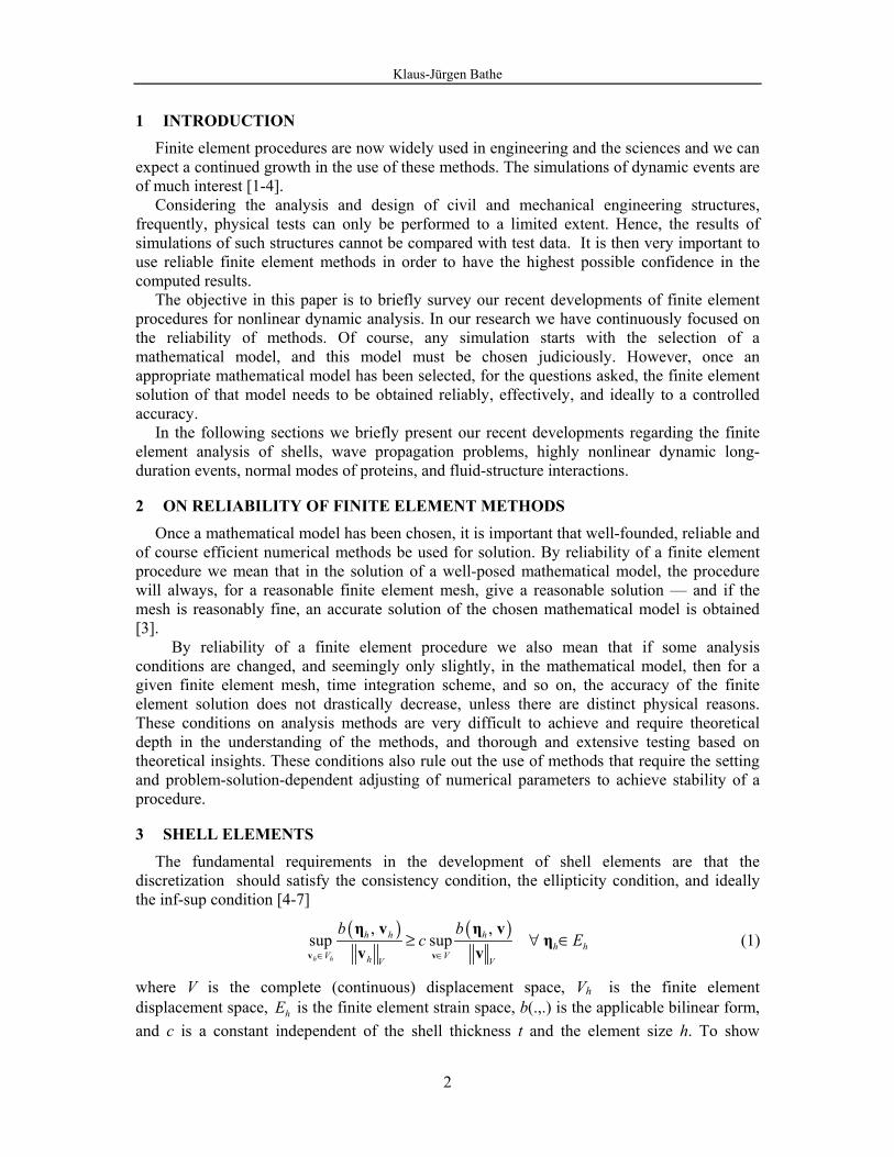
While reasonably effective quadrilateral shell elements are available, also incorporating 3D effects [9], it is a particularly difficult task to develop a general triangular 6-node shell element that is spatially isotropic, has the same degrees of freedom at every node, does not contain any instability, and converges well in membrane- and bending-dominated problems. The testing of the element should involve specific problems chosen to reveal the element properties, and in particular, shell problems based on a hyperboloid shell surface, and appropriate norms to measure the solution errors [6-8].

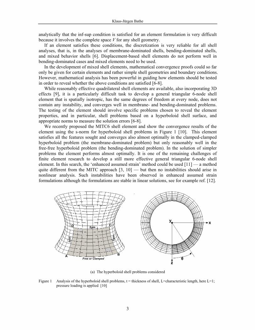
We recently proposed the MITC6 shell element and show the convergence results of the element using the s-norm for hyperboloid shell problems in Figure 1 [10]. This element satisfies all the features sought and converges also almost optimally in the clamped-clamped hyperboloid problem (the membrane-dominated problem) but only reasonably well in the free-free hyperboloid problem (the bending-dominated problem). In the solution of simpler problems the element performs almost optimally. It is one of the remaining challenges of finite element research to develop a still more effective general triangular 6-node shell element. In this search, the �enhanced assumed strain� method could be used [11] � a method quite different from the MITC approach [3, 10] � but then no instabilities should arise in nonlinear analysis. Such instabilities have been observed in enhanced assumed strain formulations although the formulations are stable in linear solutions, see for example ref. [12].

(a) The hyperboloid shell problems considered

Figure 1 Analysis of the hyperboloid shell problems, t = thickness of shell, L=characteristic length, here L=1; pressure loading is applied [10]

Klaus-Jürgen Bathe

4

(b) 8x8 element mesh used for the clamped

shell (including the boundary layer), modeling 1/8th of the shell

(c) 8x8 mesh used for free-free shell, modeling 1/8th of the shell

-1.8 -1.2 -0.6-4.0

-3.6

-3.0

-2.4

-1.8

-1.2

-0.6

0.0

log(h)

t/L=1/100t/L=1/1000t/L=1/10000

-1.8 -1.2 -0.6-4.0

-3.6

-3.0

-2.4

-1.8

-1.2

-0.6

0.0

log(h)

t/L=1/100t/L=1/1000t/L=1/10000

log

(rela

tive

erro

r)

log

(rela

tive

erro

r)

(d) Convergence results using the s-norm; left: clamped-clamped shell; right: free-free shell; the slopes of the

bold lines correspond to optimal convergence

Figure 1 (continued)

4 WAVE PROPAGATION PROBLEMS

Although in principle the finite element method can directly be applied to the solution of wave propagation problems, and indeed has been used abundantly for such analyses, a specific required accuracy in the response may be difficult to reach, and the solutions can

Klaus-Jürgen Bathe

5

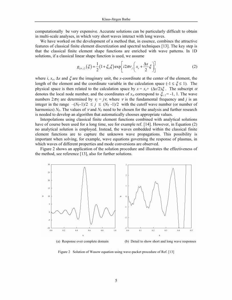
computationally be very expensive. Accurate solutions can be particularly difficult to obtain in multi-scale analyses, in which very short waves interact with long waves.

We have worked on the development of a method that, in essence, combines the attractive features of classical finite element discretization and spectral techniques [13]. The key step is that the classical finite element shape functions are enriched with wave patterns. In 1D solutions, if a classical linear shape function is used, we assume

( ) ( ) ( ),1 1 exp 22 2j ej

xg i xαα ξ ξ ξ πν ξ⎡ ∆ ⎤⎛ ⎞= + +⎜ ⎟⎢ ⎥⎝ ⎠⎣ ⎦ (2)

where i, xe, ∆x and ξ are the imaginary unit, the x-coordinate at the center of the element, the length of the element and the coordinate variable in the calculation space (-1 ≤ ξ ≤ 1). The physical space is then related to the calculation space by x = xe+ (∆x/2)ξ . The subscript α denotes the local node number, and the coordinates of xα correspond to ξ1, 2 = -1, 1. The wave numbers 2πνj are determined by νj = jν, where ν is the fundamental frequency and j is an integer in the range �(NF-1)/2 ≤ j ≤ (NF -1)/2 with the cutoff wave number (or number of harmonics) NF. The values of ν and NF need to be chosen for the analysis and further research is needed to develop an algorithm that automatically chooses appropriate values.

Interpolations using classical finite element functions combined with analytical solutions have of course been used for a long time, see for example ref. [14]. However, in Equation (2) no analytical solution is employed. Instead, the waves embedded within the classical finite element functions are to capture the unknown wave propagations. This possibility is important when solving, for example, wave equations governing the response of plasmas, in which waves of different properties and mode conversions are observed.

Figure 2 shows an application of the solution procedure and illustrates the effectiveness of the method, see reference [13], also for further solutions.

(a) Response over complete domain (b) Detail to show short and long wave responses

Figure 2 Solution of Wasow equation using wave-packet procedure of Ref. [13]

Klaus-Jürgen Bathe

6

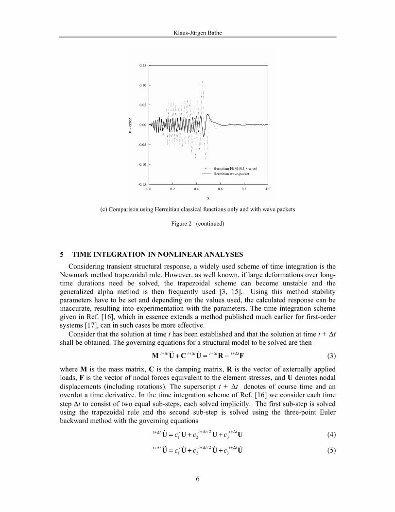
(c) Comparison using Hermitian classical functions only and with wave packets

Figure 2 (continued)

5 TIME INTEGRATION IN NONLINEAR ANALYSES

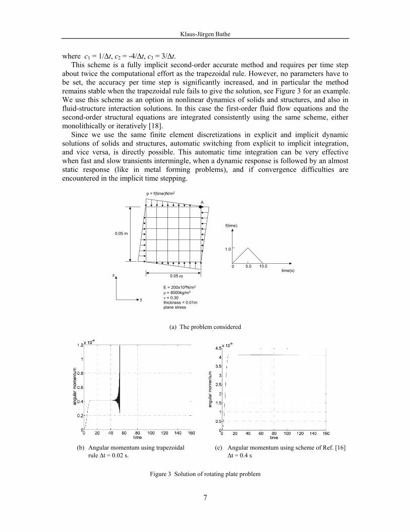
Considering transient structural response, a widely used scheme of time integration is the Newmark method trapezoidal rule. However, as well known, if large deformations over long-time durations need be solved, the trapezoidal scheme can become unstable and the generalized alpha method is then frequently used [3, 15]. Using this method stability parameters have to be set and depending on the values used, the calculated response can be inaccurate, resulting into experimentation with the parameters. The time integration scheme given in Ref. [16], which in essence extends a method published much earlier for first-order systems [17], can in such cases be more effective.

Consider that the solution at time t has been established and that the solution at time t + ∆t shall be obtained. The governing equations for a structural model to be solved are then

t t t t t t t t+∆ +∆ +∆ +∆+ = −M U C U R F!! ! (3)

where M is the mass matrix, C is the damping matrix, R is the vector of externally applied loads, F is the vector of nodal forces equivalent to the element stresses, and U denotes nodal displacements (including rotations). The superscript t + ∆t denotes of course time and an overdot a time derivative. In the time integration scheme of Ref. [16] we consider each time step ∆t to consist of two equal sub-steps, each solved implicitly. The first sub-step is solved using the trapezoidal rule and the second sub-step is solved using the three-point Euler backward method with the governing equations

/ 21 2 3t t t t tt t c c c+∆ +∆+∆ = + +U U U U! (4)

/ 21 2 3t t t t tt t c c c+∆ +∆+∆ = + +U U U U!! ! ! ! (5)

Klaus-Jürgen Bathe

7

where c1 = 1/∆t, c2 = -4/∆t, c3 = 3/∆t. This scheme is a fully implicit second-order accurate method and requires per time step

about twice the computational effort as the trapezoidal rule. However, no parameters have to be set, the accuracy per time step is significantly increased, and in particular the method remains stable when the trapezoidal rule fails to give the solution, see Figure 3 for an example. We use this scheme as an option in nonlinear dynamics of solids and structures, and also in fluid-structure interaction solutions. In this case the first-order fluid flow equations and the second-order structural equations are integrated consistently using the same scheme, either monolithically or iteratively [18].

Since we use the same finite element discretizations in explicit and implicit dynamic solutions of solids and structures, automatic switching from explicit to implicit integration, and vice versa, is directly possible. This automatic time integration can be very effective when fast and slow transients intermingle, when a dynamic response is followed by an almost static response (like in metal forming problems), and if convergence difficulties are encountered in the implicit time stepping.

E = 200x109N/m2

thickness = 0.01mplane stress

ρ = 8000kg/m3

ν = 0.30

p = f(time)N/m2

0.05 m

0.05 m

y

z

A

0 5.0 10.0time(s)

f(time)

1.0

(a) The problem considered

(b) Angular momentum using trapezoidal

rule ∆t = 0.02 s. (c) Angular momentum using scheme of Ref. [16]

∆t = 0.4 s

Figure 3 Solution of rotating plate problem

Klaus-Jürgen Bathe

8

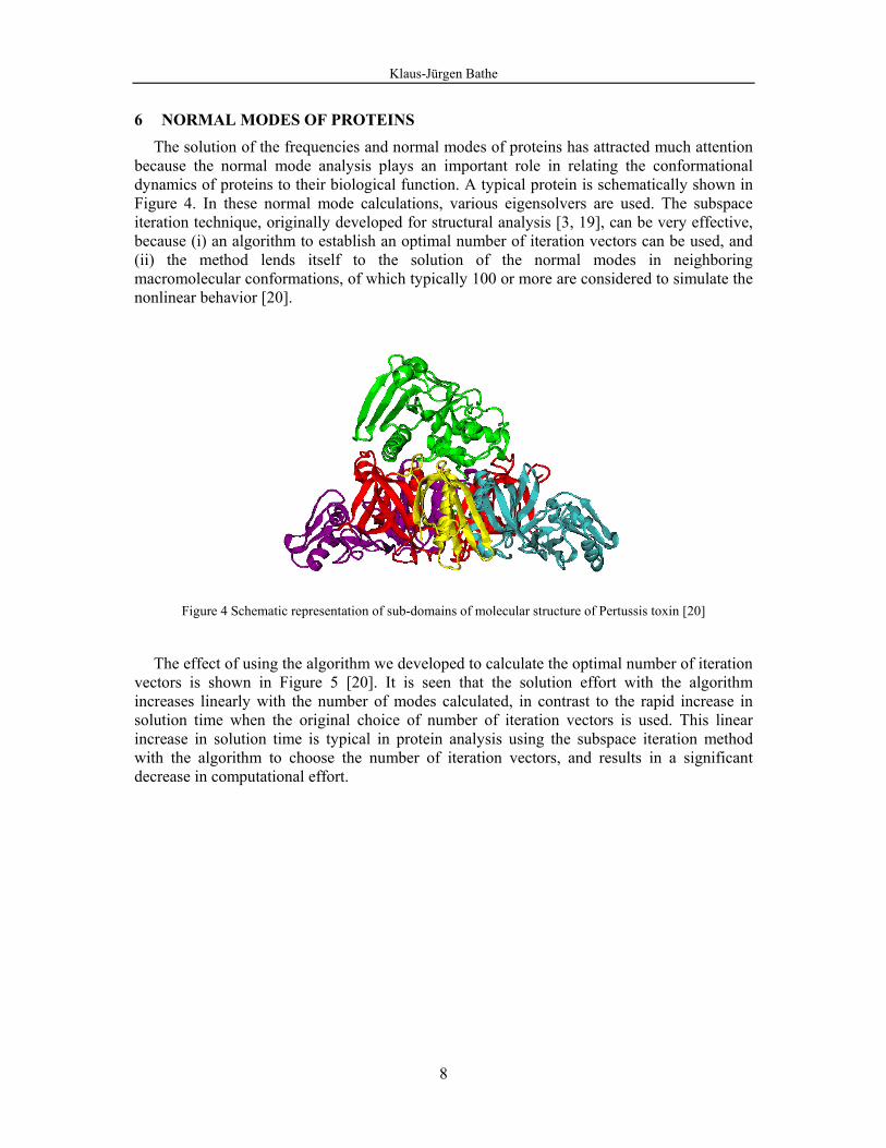
6 NORMAL MODES OF PROTEINS The solution of the frequencies and normal modes of proteins has attracted much attention

because the normal mode analysis plays an important role in relating the conformational dynamics of proteins to their biological function. A typical protein is schematically shown in Figure 4. In these normal mode calculations, various eigensolvers are used. The subspace iteration technique, originally developed for structural analysis [3, 19], can be very effective, because (i) an algorithm to establish an optimal number of iteration vectors can be used, and (ii) the method lends itself to the solution of the normal modes in neighboring macromolecular conformations, of which typically 100 or more are considered to simulate the nonlinear behavior [20].

Figure 4 Schematic representation of sub-domains of molecular structure of Pertussis toxin [20]

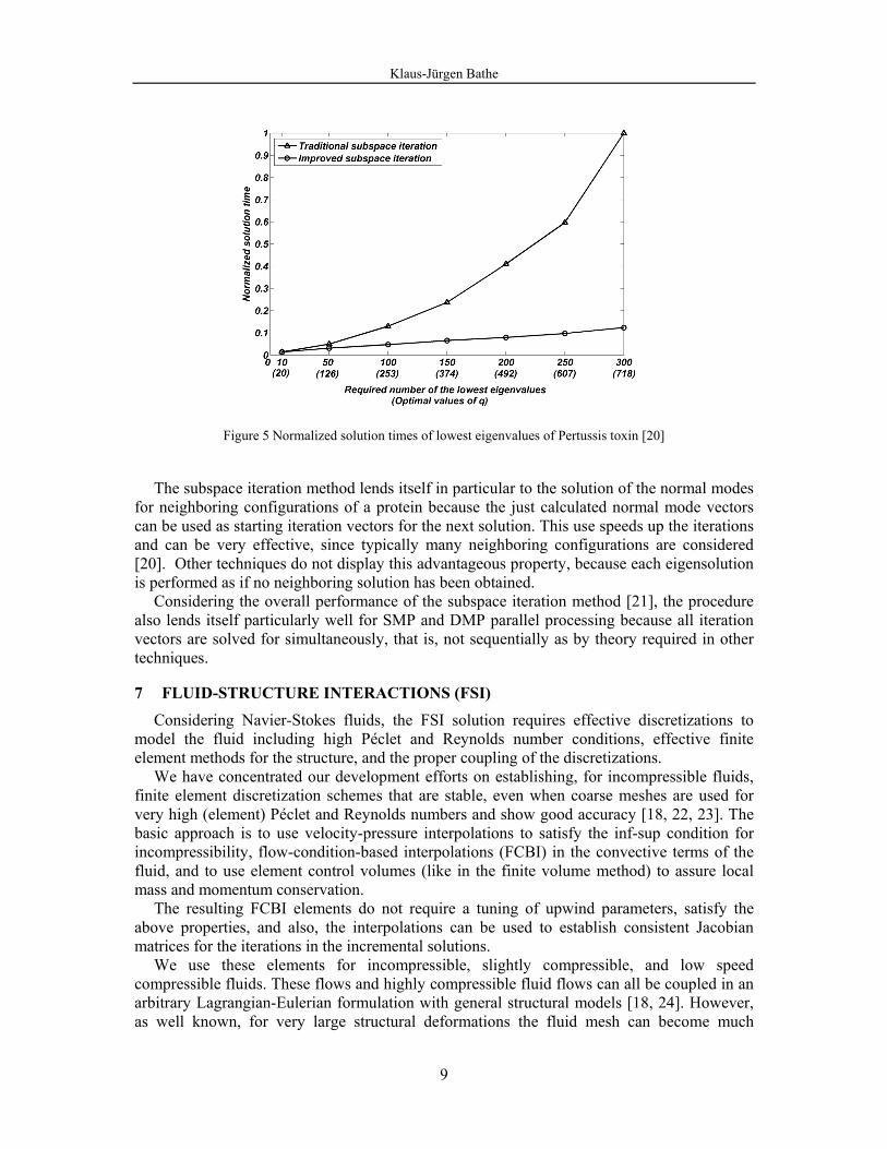
The effect of using the algorithm we developed to calculate the optimal number of iteration

vectors is shown in Figure 5 [20]. It is seen that the solution effort with the algorithm increases linearly with the number of modes calculated, in contrast to the rapid increase in solution time when the original choice of number of iteration vectors is used. This linear increase in solution time is typical in protein analysis using the subspace iteration method with the algorithm to choose the number of iteration vectors, and results in a significant decrease in computational effort.

Klaus-Jürgen Bathe

9

Figure 5 Normalized solution times of lowest eigenvalues of Pertussis toxin [20]

The subspace iteration method lends itself in particular to the solution of the normal modes

for neighboring configurations of a protein because the just calculated normal mode vectors can be used as starting iteration vectors for the next solution. This use speeds up the iterations and can be very effective, since typically many neighboring configurations are considered [20]. Other techniques do not display this advantageous property, because each eigensolution is performed as if no neighboring solution has been obtained.

Considering the overall performance of the subspace iteration method [21], the procedure also lends itself particularly well for SMP and DMP parallel processing because all iteration vectors are solved for simultaneously, that is, not sequentially as by theory required in other techniques.

7 FLUID-STRUCTURE INTERACTIONS (FSI)

Considering Navier-Stokes fluids, the FSI solution requires effective discretizations to model the fluid including high Péclet and Reynolds number conditions, effective finite element methods for the structure, and the proper coupling of the discretizations.

We have concentrated our development efforts on establishing, for incompressible fluids, finite element discretization schemes that are stable, even when coarse meshes are used for very high (element) Péclet and Reynolds numbers and show good accuracy [18, 22, 23]. The basic approach is to use velocity-pressure interpolations to satisfy the inf-sup condition for incompressibility, flow-condition-based interpolations (FCBI) in the convective terms of the fluid, and to use element control volumes (like in the finite volume method) to assure local mass and momentum conservation.

The resulting FCBI elements do not require a tuning of upwind parameters, satisfy the above properties, and also, the interpolations can be used to establish consistent Jacobian matrices for the iterations in the incremental solutions.

We use these elements for incompressible, slightly compressible, and low speed compressible fluids. These flows and highly compressible fluid flows can all be coupled in an arbitrary Lagrangian-Eulerian formulation with general structural models [18, 24]. However, as well known, for very large structural deformations the fluid mesh can become much

Klaus-Jürgen Bathe

10

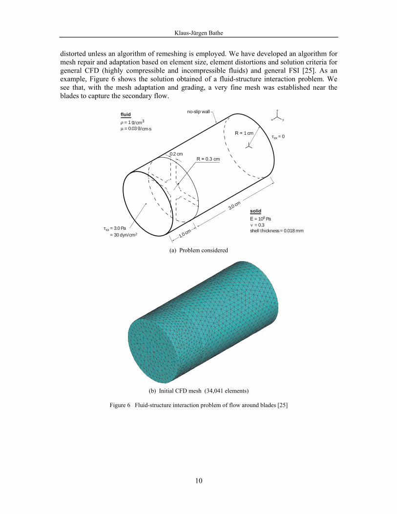
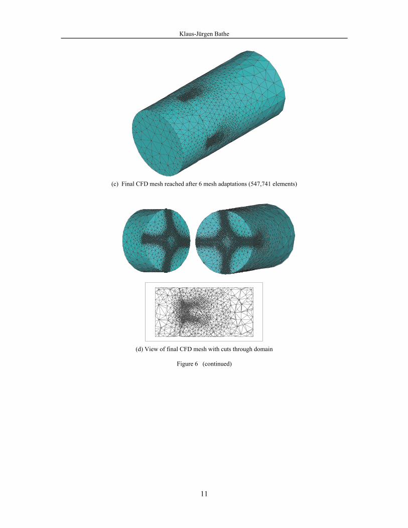
distorted unless an algorithm of remeshing is employed. We have developed an algorithm for mesh repair and adaptation based on element size, element distortions and solution criteria for general CFD (highly compressible and incompressible fluids) and general FSI [25]. As an example, Figure 6 shows the solution obtained of a fluid-structure interaction problem. We see that, with the mesh adaptation and grading, a very fine mesh was established near the blades to capture the secondary flow.

z

fluidρ = 1 g/cm3

µ = 0.03 g/cm.s

no-slip wall

R = 1 cm

R = 0.3 cm

1.0 cm

0.2 cm

τxx = 3.0 Pa

= 30 dyn/cm2

solidE = 108 Pa ν = 0.3shell thickness = 0.018 mm

3.0 cm

τxx = 0

x y

(a) Problem considered

(b) Initial CFD mesh (34,041 elements)

Figure 6 Fluid-structure interaction problem of flow around blades [25]

Klaus-Jürgen Bathe

11

(c) Final CFD mesh reached after 6 mesh adaptations (547,741 elements)

(d) View of final CFD mesh with cuts through domain

Figure 6 (continued)

Klaus-Jürgen Bathe

12

VELOCITY�

TIME 4.000�

5.04�7�

4.55�0�

3.850�

3.150�

2.450�

1.75�0�

1.050�

0.350�

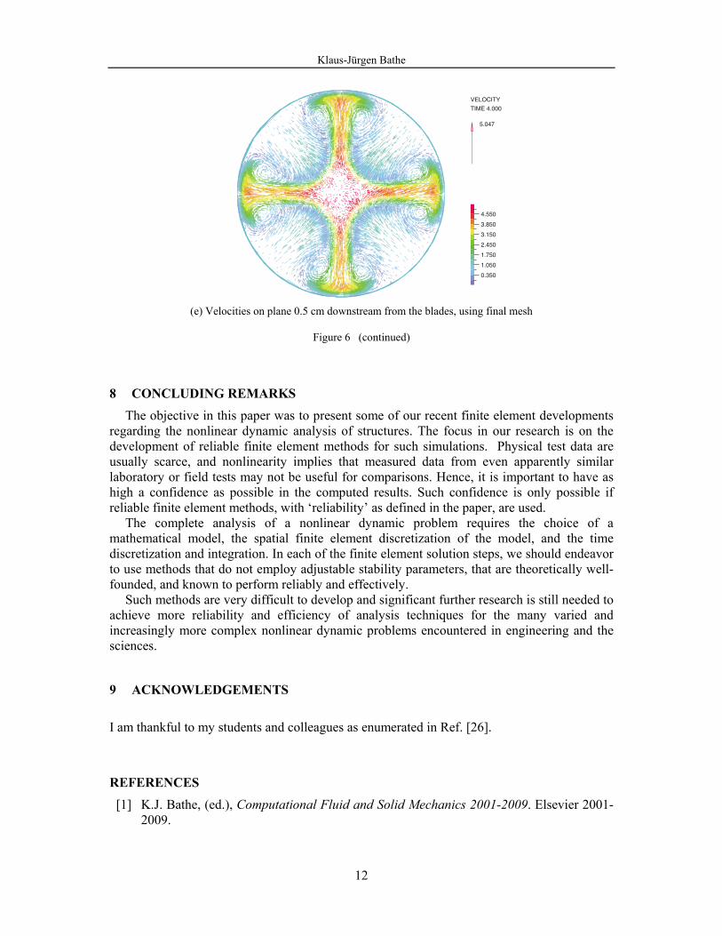
(e) Velocities on plane 0.5 cm downstream from the blades, using final mesh

Figure 6 (continued)

8 CONCLUDING REMARKS The objective in this paper was to present some of our recent finite element developments

regarding the nonlinear dynamic analysis of structures. The focus in our research is on the development of reliable finite element methods for such simulations. Physical test data are usually scarce, and nonlinearity implies that measured data from even apparently similar laboratory or field tests may not be useful for comparisons. Hence, it is important to have as high a confidence as possible in the computed results. Such confidence is only possible if reliable finite element methods, with �reliability� as defined in the paper, are used.

The complete analysis of a nonlinear dynamic problem requires the choice of a mathematical model, the spatial finite element discretization of the model, and the time discretization and integration. In each of the finite element solution steps, we should endeavor to use methods that do not employ adjustable stability parameters, that are theoretically well-founded, and known to perform reliably and effectively.

Such methods are very difficult to develop and significant further research is still needed to achieve more reliability and efficiency of analysis techniques for the many varied and increasingly more complex nonlinear dynamic problems encountered in engineering and the sciences.

9 ACKNOWLEDGEMENTS

I am thankful to my students and colleagues as enumerated in Ref. [26].

REFERENCES [1] K.J. Bathe, (ed.), Computational Fluid and Solid Mechanics 2001-2009. Elsevier 2001-

2009.

Klaus-Jürgen Bathe

13

[2] O.C. Zienkiewicz and R.L. Taylor, The Finite Element Method. Butterworth-Heinemann, 2005.

[3] K.J. Bathe, Finite Element Procedures. Prentice Hall, 1996, amazon.com.

[4] K.J. Bathe, The finite element method. Chapter in Encyclopedia of Computer Science and Engineering, B. Wah (ed.), J. Wiley and Sons, 2009.

[5] K.J. Bathe, The inf-sup condition and its evaluation for mixed finite element methods, Computers & Structures, 79, 243-252, 971, 2001.

[6] D. Chapelle and K.J. Bathe, The Finite Element Analysis of Shells � Fundamentals. Springer, 2003.

[7] J.F. Hiller and K.J. Bathe, Measuring convergence of mixed finite element discretizations: An application to shell structures, Computers & Structures, 81, 639-654, 2003.

[8] D. Chapelle and K.J. Bathe, Fundamental considerations for the finite element analysis of shell structures, Computers & Structures, 66(1), 19-36, 1998.

[9] D.N. Kim and K.J. Bathe, A 4-node 3D-shell element to model shell surface tractions and incompressible behavior, Computers & Structures, 86, 2027-2041, 2008.

[10] D.N. Kim and K.J. Bathe, A new triangular six-node shell element, Computers & Structures, to appear.

[11] J.C. Simo and M.S. Rifai, A class of mixed assumed strain methods and the method of incompatible modes, Int. Journal for Numerical Methods in Engineering, 29, 1595-1638, 1990.

[12] D. Pantuso and K.J. Bathe, On the stability of mixed finite elements in large strain analysis of incompressible solids, Finite Elements in Analysis and Design, 28, 83-104, 1997.

[13] H. Kohno, K.J. Bathe, and J.C. Wright, A finite element procedure for multiscale wave equations with application to plasma waves, submitted for publication.

[14] R.J. Astley, Wave envelope and infinite elements for acoustical radiation. Int. Journal for Numerical Methods in Fluids, 3, 507-526, 1983.

[15] J. Chung and G.M. Hulbert, A time integration algorithm for structural dynamics with improved numerical dissipation � the generalized alpha method, Journal of Applied Mechanics - Transactions of the ASME, 60, 371-375, 1993.

[16] K.J. Bathe, Conserving energy and momentum in nonlinear dynamics: A simple implicit time integration scheme, Computers & Structures, 85, 437-445, 2007.

[17] R.E. Bank, W.M. Coughran, Jr., W Fichtner, E.H. Grosse, D.J. Rose, and R.K. Smith, Transient simulation of silicon devices and circuits, IEEE Trans. 1985, CAD-4(4):436-451.

[18] K.J. Bathe and H. Zhang, Finite element developments for general fluid flows with structural interactions, Int. Journal for Numerical Methods in Engineering, 60, 213-232, 2004.

Klaus-Jürgen Bathe

14

[19] K.J. Bathe, Solution Methods for Large Generalized Eigenvalue Problems in Structural Engineering, Report UCSESM 71-20, Department of Civil Engineering, University of California, Berkeley, November 1971.

[20] R.S. Sedeh, M. Bathe, and K.J. Bathe, The subspace iteration method in protein normal mode analysis, J. Computational Chemistry, in press.

[21] K.J. Bathe, The subspace iteration method revisited, in preparation.

[22] K.J. Bathe and H. Zhang, A flow-condition-based interpolation finite element procedure for incompressible fluid flows, Computers & Structures, 80, 1267-1277, 2002.

[23] H. Kohno and K.J. Bathe, A flow-condition-based interpolation finite element procedure for triangular grids, Int. Journal for Numerical Methods in Fluids, 51, 673-699, 2006.

[24] K.J. Bathe and G.A. Ledezma, Benchmark problems for incompressible fluid flows with structural interactions, Computers & Structures, 85, 628-644, 2007.

[25] K.J. Bathe and H. Zhang, A mesh adaptivity procedure for CFD and fluid-structure interactions, Computers & Structures, in press.

[26] K.J. Bathe, To Enrich Life, ISBN 978-0-9790049-2-6, amazon.com.