ADVANCES IN SURFACE PENETRATINGTECHNOLOGIES FOR IMAGING, DETECTION, AND

CLASSIFICATION

by

Jay A. Marble

A dissertation submitted in partial fulfillmentof the requirements for the degree of

Doctor of Philosophy(Electrical Engineering: Systems)

in The University of Michigan2007

Doctoral Committee:

Professor Alfred O. Hero III, Co-ChairProfessor Andrew E. Yagle, Co-ChairProfessor Eric MichielssenAssociate Professor Mahta Moghaddam

Jay A. Marblec© 2007

All rights reserved.

To: the Environmental Research Institute of Michigan (ERIM)

ii

ACKNOWLEDGMENTS

The author gratefully acknowledges the support of and collaboration with the U.S.

Army’s Night Vision and Electronic Sensor Directorate (NVESD). He also wishes to

thank the Army Research Office (ARO) for their support of the Multi-modal, Adaptive

Target Detection and Classification MURI (project number DAAD-19-02-1-0262). The

views and conclusions contained in this document are those of the author and should not

be interpreted as representing official policies, either expressed or implied, of NVESD,

ARO, or the United States government.

For assistance with data processing, problem insights, andassistance with results

thanks goes to Mehrdad Soumekh, Raviv Raich, Hakan Bagci, and Doron Blatt. For

mentorship and career direction thanks goes to John Ackenhusen of General Dynamics

- Advanced Information Systems (Ann Arbor) and Steve Bishop of NVESD. For use of

their data and facilities thanks goes to Waymond Scott, Gregg Larson, and Jim McClellen

of the Georgia Institute of Technology. For guidance in the first two years of research,

thanks goes to Professor Andy Yagle. Thanks also to Professor Al Hero for challenging

the author to approach academic problems in a more rigorous,theoretical way. Thanks

to the E&M members of the committee Professor Eric Michielssen and Professor Mahta

Moghaddam for their valuable insight.

For listening to the author complain about how much work it isto get a Ph.D., grateful

thanks is due to his many friends, the Christian Faith Group, and especially Patrick Spicer.

For emotional support throughout this five year life chapterthe author thanks his family:

James, Joyce, Jon, and Colleen Marble. For perseverance in study and the ability to

iii

understand anything at all, the author humbly wishes to thank the Creator.

iv

TABLE OF CONTENTS

DEDICATION . . . . . . . . . . . . . . . . . . . . . . . . . . . . . . . . . . . ii

ACKNOWLEDGMENTS . . . . . . . . . . . . . . . . . . . . . . . . . . . . . iii

LIST OF FIGURES . . . . . . . . . . . . . . . . . . . . . . . . . . . . . . . . viii

LIST OF TABLES . . . . . . . . . . . . . . . . . . . . . . . . . . . . . . . . . xii

LIST OF APPENDICES . . . . . . . . . . . . . . . . . . . . . . . . . . . . . . xiii

ABSTRACT . . . . . . . . . . . . . . . . . . . . . . . . . . . . . . . . . . . . . xiv

CHAPTER

I. INTRODUCTION . . . . . . . . . . . . . . . . . . . . . . . . . . . . . . 11.1 Contributions Made . . . . . . . . . . . . . . . . . . . . . . . . . 21.2 Outline of Dissertation . . . . . . . . . . . . . . . . . . . . . . . . 41.3 List of Publications . . . . . . . . . . . . . . . . . . . . . . . . . 5

II. OVERVIEW OF THE FIELD . . . . . . . . . . . . . . . . . . . . . . . 72.1 Historical Background . . . . . . . . . . . . . . . . . . . . . . . . 7

2.1.1 Foliage Penetrating Radar . . . . . . . . . . . . . . . . 72.1.2 Unexploded Ordnance Detection . . . . . . . . . . . . . 72.1.3 Landmines . . . . . . . . . . . . . . . . . . . . . . . . 82.1.4 Emerging Applications . . . . . . . . . . . . . . . . . . 10

2.2 Landmine Detection and Classification Research . . . . . . . . .. 102.2.1 Low Signal-to-Noise Ratio . . . . . . . . . . . . . . . . 122.2.2 False Alarm Rejection . . . . . . . . . . . . . . . . . . 12

2.3 See-Through-Wall Radar Imaging . . . . . . . . . . . . . . . . . . 14III. NON-STATISTICAL APPROACHES . . . . . . . . . . . . . . . . . . . 16

3.1 Imaging Using Ground Penetrating Radar . . . . . . . . . . . . . 163.1.1 Size and Depth Estimation Algorithm . . . . . . . . . . 183.1.2 Algorithm Validation - Repeatability Study . . . . . . . 22

3.2 Pseudo Imaging . . . . . . . . . . . . . . . . . . . . . . . . . . . 243.2.1 Algorithm Discription . . . . . . . . . . . . . . . . . . 253.2.2 Results on Simulated Data . . . . . . . . . . . . . . . . 283.2.3 Results on Real Data . . . . . . . . . . . . . . . . . . . 30

v

3.2.4 Applications . . . . . . . . . . . . . . . . . . . . . . . 303.2.5 Pseudo Imaging Conclusions . . . . . . . . . . . . . . . 33

3.3 Subspace Methods . . . . . . . . . . . . . . . . . . . . . . . . . . 343.3.1 Depth and Shape Information . . . . . . . . . . . . . . 343.3.2 TheΛ andW Basis Functions . . . . . . . . . . . . . . 363.3.3 Subspace Identification . . . . . . . . . . . . . . . . . . 383.3.4 Shape Identification . . . . . . . . . . . . . . . . . . . 413.3.5 Subspace Method Conclusions . . . . . . . . . . . . . . 43

IV. STATISTICAL APPROACHES . . . . . . . . . . . . . . . . . . . . . . 454.1 Multimodal Detection . . . . . . . . . . . . . . . . . . . . . . . . 45

4.1.1 Multimodal Landmine Detection . . . . . . . . . . . . . 454.1.2 Adapting to the Environment . . . . . . . . . . . . . . . 484.1.3 Detection Performance . . . . . . . . . . . . . . . . . . 504.1.4 Multimodal Summary . . . . . . . . . . . . . . . . . . 52

4.2 Bayes Networks . . . . . . . . . . . . . . . . . . . . . . . . . . . 53V. SENSOR SCHEDULING . . . . . . . . . . . . . . . . . . . . . . . . . . 56

5.1 Single Confirmation Sensor - Active Sensing . . . . . . . . . . . .565.1.1 Sensor Management using Active Sensing . . . . . . . . 585.1.2 Scanning Sensor Simulations . . . . . . . . . . . . . . . 605.1.3 Confirmation Sensor Models . . . . . . . . . . . . . . . 625.1.4 Clutter Rejection Example - Myopic . . . . . . . . . . . 645.1.5 Accounting for Processing Time . . . . . . . . . . . . . 685.1.6 Single Confirmation Sensor Summary . . . . . . . . . . 71

5.2 Multiple Confirmation Sensors - Reinforcement Learning . .. . . 715.2.1 Landmine Detection Technologies . . . . . . . . . . . . 735.2.2 Landmine Types and Responses . . . . . . . . . . . . . 745.2.3 Sensor Scheduling Policy . . . . . . . . . . . . . . . . 755.2.4 Multiple Confirmation Sensor Summary . . . . . . . . . 77

VI. SURFACE PENETRATING RADAR IMAGING . . . . . . . . . . . . 786.1 Backpropagation Radar Imaging . . . . . . . . . . . . . . . . . . 79

6.1.1 Inverse Problems . . . . . . . . . . . . . . . . . . . . . 816.1.2 Backpropagation as an Inverse Problem . . . . . . . . . 82

6.2 Wavenumber Migration . . . . . . . . . . . . . . . . . . . . . . . 846.2.1 Landmine Imaging with Wavenumber Migration . . . . 856.2.2 Matrix Implementation . . . . . . . . . . . . . . . . . . 91

6.3 Exploiting Sparsity as Prior Knowledge . . . . . . . . . . . . . .. 94VII. ITERATIVE REDEPLOYMENT OF IMAGING AND SENSING . . . 98

7.1 Phenomenology of See-Through-Wall Radar . . . . . . . . . . . . 987.2 The Outer Wall Problem . . . . . . . . . . . . . . . . . . . . . . . 103

7.2.1 Point Target Simulations . . . . . . . . . . . . . . . . . 1057.2.2 Wall Phase Determination and Correction . . . . . . . . 1087.2.3 Outer Wall Conclusion . . . . . . . . . . . . . . . . . . 115

7.3 The Inner Wall Problem . . . . . . . . . . . . . . . . . . . . . . . 1167.3.1 Inner Wall Simulation . . . . . . . . . . . . . . . . . . 1167.3.2 Layout Mapping . . . . . . . . . . . . . . . . . . . . . 120

vi

7.3.3 Inner Wall Conclusion . . . . . . . . . . . . . . . . . . 1227.4 I.R.I.S. Adaptive Imaging . . . . . . . . . . . . . . . . . . . . . . 122

7.4.1 Numerical Simulation . . . . . . . . . . . . . . . . . . 1257.4.2 Convergence . . . . . . . . . . . . . . . . . . . . . . . 128

VIII. CONCLUSION . . . . . . . . . . . . . . . . . . . . . . . . . . . . . . . 1328.1 Discussion of Results . . . . . . . . . . . . . . . . . . . . . . . . 1328.2 Suggestions for Further Research . . . . . . . . . . . . . . . . . . 134

APPENDICES . . . . . . . . . . . . . . . . . . . . . . . . . . . . . . . . . . . 135

BIBLIOGRAPHY . . . . . . . . . . . . . . . . . . . . . . . . . . . . . . . . . 161

vii

LIST OF FIGURES

1.1 The Surface Penetrating Problem Generalized . . . . . . . . .. . . . . . 2

3.1 A TM-62M, Metal Cased Landmine (Dimensions: hgt. - 6”, dia. - 13”) . . 173.2 Observed Signature of a TM-62M (Depth: 6” to top) . . . . . . .. . . . . 183.3 Image After Wavenumber Migration - Size of reflections reveals the depth,

height, and diameter of the landmine. . . . . . . . . . . . . . . . . . . .. 183.4 Binarized Image of Fig. 3.3 - Reflections from the top and bottom of the

landmine are visible. . . . . . . . . . . . . . . . . . . . . . . . . . . . . . 193.5 Focused Image of TM-62M Landmine . . . . . . . . . . . . . . . . . . . 203.6 Fig.3.5 After Thresholding . . . . . . . . . . . . . . . . . . . . . . . .. 203.7 The negative of the focused image converts the shadow region into a

bright one. . . . . . . . . . . . . . . . . . . . . . . . . . . . . . . . . . . 213.8 Shadow region is automatically identified and labeled 1 by the algorithm. . 213.9 Characteristic Hyperbolic Signature of a Landmine Measured by GPR . . 253.10 Steps of the HFT Applied to a Simulated Hyperbolic Signature . . . . . . 293.11 Steps of the HFT Applied to an Actual Hyperbolic Signature . . . . . . . 313.12 Italian VS1.6 Landmine at 6” Depth . . . . . . . . . . . . . . . . . .. . 323.13 The HFT Applied to Every Point of the Image . . . . . . . . . . . .. . . 323.14 The 20% Brightest Pixels of the Transformed Data . . . . . . .. . . . . . 333.15 Vertical Standard Deviation Showing Location of the Most Hyperbolic

Signatures . . . . . . . . . . . . . . . . . . . . . . . . . . . . . . . . . . 343.16 Typical EMI Spatial Signal - 1D . . . . . . . . . . . . . . . . . . . . .. . 363.17 TheΛ andW Basis Functions . . . . . . . . . . . . . . . . . . . . . . . . 373.18 Signals from Spheres at Canonical Depths . . . . . . . . . . . . .. . . . 383.19 Canonical Objects at Same Depth . . . . . . . . . . . . . . . . . . . . .. 42

4.1 Estimated Joint Probability Density Functions . . . . . . .. . . . . . . . 464.2 Marginalized Probability Density Functions of Mid-depth, Metal Cased

Landmines . . . . . . . . . . . . . . . . . . . . . . . . . . . . . . . . . . 474.3 Signatures from a Mid-depth, Metal Cased Landmine . . . . . .. . . . . 484.4 PDFs of EMI and GPR pixels from mid-depth buried metal landmines.

(left) Lane material is clay. (right) Lane material is gravel. . . . . . . . . . 494.5 Inverse Mapping from Reflection Coefficient to Dielectric Permittivity . . 504.6 Multi-modal Versus Single Mode MAP Detection Algorithms - Multi-

modal processing has a clear advantage. . . . . . . . . . . . . . . . . .. 51

viii

4.7 Multi-modal MAP Detector Trained and Applied to Clay BackgroundCompared to a Generalized Detector Trained and Applied to ClayandGravel Backgrounds . . . . . . . . . . . . . . . . . . . . . . . . . . . . . 52

4.8 A Bayesian Network Structure for the Burglar Alarm Problem. . . . . . . 544.9 A Bayesian Network Structure for the Landmine Problem . . .. . . . . . 55

5.1 Proposed Architecture for Applying Sensor Management to a VehicleMounted Landmine Detection System . . . . . . . . . . . . . . . . . . . 57

5.2 Simulated Signature of an EMI Scanning Sensor Array . . . .. . . . . . 615.3 Simulated Signature of a GPR Scanning Sensor Array . . . . .. . . . . . 615.4 A Virtual Test Lane - Locations of simulated landmines and clutter objects 625.5 Simulated Signatures of the Iron Clutter Object . . . . . . . .. . . . . . . 645.6 Type Probabilities: a) Prior Distribution b) After Scanning Sensors c) Af-

ter Confirmation Sensor. The correct type for this case is Type9 (IronClutter). . . . . . . . . . . . . . . . . . . . . . . . . . . . . . . . . . . . 65

5.7 Myopic Sensor Actions Taken for Iron Clutter Object . . . . .. . . . . . 665.8 Modified Decision Statistic Based on Balancing Information Gain and

Required Processing Time . . . . . . . . . . . . . . . . . . . . . . . . . 695.9 Sensor Actions Taken for Iron Clutter Object with Time Monitoring . . . . 695.10 Sensors of the Georgia Tech Three Sensor Data Collection: EMI, GPR,

and Seismic Vibrometer . . . . . . . . . . . . . . . . . . . . . . . . . . . 735.11 Decision Tree for Sensor Management . . . . . . . . . . . . . . . .. . . 76

6.1 Block Diagram of the Wavenumber Migration Process . . . . . .. . . . . 866.2 The antennae and ground may be viewed as a black box. . . . . .. . . . . 886.3 Geometry of Signature Collection . . . . . . . . . . . . . . . . . . . .. . 906.4 Simulated Signature . . . . . . . . . . . . . . . . . . . . . . . . . . . . . 906.5 STW Radar Example: Wavenumber Migration . . . . . . . . . . . . . .. 946.6 Block Diagram of Reverse Wavenumber Migration - An approximation to

the Forward Operator . . . . . . . . . . . . . . . . . . . . . . . . . . . . 966.7 Block Diagram of Wavenumber Migration . . . . . . . . . . . . . . . .. 976.8 STW Radar Example: Sparse Reconstruction . . . . . . . . . . . . . .. . 97

7.1 Geometrical Optics Wall Model . . . . . . . . . . . . . . . . . . . . . .. 1007.2 Geometrical Optics Bistatic Model . . . . . . . . . . . . . . . . . . .. . 1027.3 Three Point Scatterer Simulations . . . . . . . . . . . . . . . . . .. . . . 1057.4 Point Simulation - No Wall . . . . . . . . . . . . . . . . . . . . . . . . . 1067.5 Point Simualtion - Wall Inserted . . . . . . . . . . . . . . . . . . . .. . . 1067.6 Estimated and True Phase . . . . . . . . . . . . . . . . . . . . . . . . . . 1107.7 Image After Correction with Dual Phase Approach . . . . . . . .. . . . . 1117.8 Convergence of Parameterx1 . . . . . . . . . . . . . . . . . . . . . . . . 1147.9 Convergence of Parameterx2 . . . . . . . . . . . . . . . . . . . . . . . . 1147.10 Image After Correction with the Dual Frequency Approach. . . . . . . . 1157.11 Dihedral Scattering Center . . . . . . . . . . . . . . . . . . . . . . . .. 1187.12 Inner Wall Simulation - Bottom Illumination . . . . . . . . . .. . . . . . 119

ix

7.13 Inner Wall Simulation - Left Illumination . . . . . . . . . . .. . . . . . . 1197.14 Detected Inner Walls - Bottom Illumination . . . . . . . . . . .. . . . . . 1217.15 Detected Inner Walls - Left Illumination . . . . . . . . . . . .. . . . . . 1217.16 2D scenario used to illustrate the IRIS approach. Room is10× 10 meters

and a SAR sensor with 1 meter baseline can be placed at any positionparallel to top or bottom walls at exterior of building. . . . .. . . . . . . 123

7.17 Iterative reconstruction of building interior illustrated in Fig. 7.16 after 10iterations and a full 10 meter baseline (left) and 1 meter baseline (right)monostatic SAR illuminator/sensor. . . . . . . . . . . . . . . . . . . .. . 124

7.18 Confidence Map (left) and Entropy Map (right) associatedwith the 1 me-ter baseline image reconstruction shown in Fig. 7.17. . . . . .. . . . . . . 126

7.19 The information gain field is computed by simulating thevariability of theRF spectrum that a virtual transmitter in the vicinity of a pixel of interest(circle 1 in left panel) would generate at different locations at the exteriorof the building. At right are the induced RF fields generated bya virtualtransmitter at the reference position (circle 1), cross-range (circle 2), andrange (circle 3) perturbations. . . . . . . . . . . . . . . . . . . . . . . .. 127

7.20 Virtual transmitter locations and the induced information gain fields foriteration 2 and 3 of IRIS for the scenario illustrated in Fig. 7.16. . . . . . . 127

7.21 Comparison between final IRIS reconstruction after 4 iterations with 1meter baseline SAR deployments (shown by black arrows) versus oneshot IRIS reconstruction using 10 meter baseline. In both cases the re-verse wavenumber migration model with EM implementation ofMAPalgorithm has been used. . . . . . . . . . . . . . . . . . . . . . . . . . . 128

7.22 Image from360o Aperture . . . . . . . . . . . . . . . . . . . . . . . . . . 1297.23 Image from IRIS . . . . . . . . . . . . . . . . . . . . . . . . . . . . . . . 1307.24 Convergence of Imaged Scene . . . . . . . . . . . . . . . . . . . . . . . .131

A.1 The EM61 Metal Detector . . . . . . . . . . . . . . . . . . . . . . . . . . 137A.2 Transmitter Current Waveform . . . . . . . . . . . . . . . . . . . . . . .138A.3 Phenomenology of Induced Dipole Sources . . . . . . . . . . . . .. . . . 140A.4 Receiver Schematic Diagram . . . . . . . . . . . . . . . . . . . . . . . . 143A.5 EMI Spatial Response . . . . . . . . . . . . . . . . . . . . . . . . . . . . 145

B.1 Electron Energy Levels in a Cesium atom in the presence of a DC Mag-netic Field . . . . . . . . . . . . . . . . . . . . . . . . . . . . . . . . . . 147

B.2 Effect of an Iron Object on the Earth’s Magnetic Field . . . .. . . . . . . 148B.3 Simulated Spatial Signal from a magnetometer . . . . . . . . . .. . . . . 149B.4 Signatures of Buried UXO on a Magnetometer . . . . . . . . . . . . . .. 149B.5 Along Track UXO Signatures on a Magnetometer Sensor . . . . .. . . . 149

C.1 Plastic Cased Anti-tank Landmine . . . . . . . . . . . . . . . . . . . . .151C.2 Compton Linear Attenuation . . . . . . . . . . . . . . . . . . . . . . . . 153C.3 Photo-electric Attenuation . . . . . . . . . . . . . . . . . . . . . . . .. . 154C.4 Compton Scattering . . . . . . . . . . . . . . . . . . . . . . . . . . . . . 155

x

C.5 Proposed X-ray Backscatter Imaging Scanner . . . . . . . . . . . .. . . 155C.6 Ratio of Compton to Photo-electric Absorption . . . . . . . . . . .. . . . 157C.7 Collision Cross Section of Compton Events . . . . . . . . . . . . . . . .159

xi

LIST OF TABLES

3.1 Summary of Estimates - All units in inches. . . . . . . . . . . . .. . . . 233.2 Norm After Projection into Subspaces (No Noise) . . . . . . .. . . . . . 403.3 Norm After Projection into Subspaces (Noise Standard Deviation: 0.01) . 403.4 Norm After Projection into Subspaces (Noise Standard Deviation: 0.05) . 413.5 Norm After Projection into Subspaces (Noise Standard Deviation: 0.3) . . 413.6 Shape Polarizabilities . . . . . . . . . . . . . . . . . . . . . . . . . . .. 423.7 Polarizability Estimates (No Noise) . . . . . . . . . . . . . . . .. . . . . 433.8 Polarizability Estimates (Noise Var: 0.01) . . . . . . . . . .. . . . . . . 433.9 Polarizability Estimates (Noise Var: 0.05) . . . . . . . . . .. . . . . . . 44

5.1 Averages . . . . . . . . . . . . . . . . . . . . . . . . . . . . . . . . . . . 635.2 Variances . . . . . . . . . . . . . . . . . . . . . . . . . . . . . . . . . . . 635.3 Confusion Matrix for Scanning Sensors . . . . . . . . . . . . . . . .. . . 665.4 Confusion Matrix after Confirmation Sensors . . . . . . . . . . . .. . . . 685.5 Processing Times Associated with Each Sensor . . . . . . . . .. . . . . . 695.6 Confusion Matrix after Confirmation Sensors with Time Constraint . . . . 705.7 Qualitative Description of Sensor Response to Various Landmine/Clutter

Types . . . . . . . . . . . . . . . . . . . . . . . . . . . . . . . . . . . . . 755.8 The Optimal Policy . . . . . . . . . . . . . . . . . . . . . . . . . . . . . 76

C.1 Detector Distances . . . . . . . . . . . . . . . . . . . . . . . . . . . . . . 157

xii

LIST OF APPENDICES

A. ELECTROMAGNETIC INDUCTION (EMI) SENSORS . . . . . . . . . . 136

B. MAGNETOMETERS . . . . . . . . . . . . . . . . . . . . . . . . . . . . 146

C. X-RAY BACKSCATTER . . . . . . . . . . . . . . . . . . . . . . . . . . 151

xiii

ABSTRACT

ADVANCES IN SURFACE PENETRATING TECHNOLOGIES FOR IMAGING,

DETECTION, AND CLASSIFICATION

by

Jay A. Marble

Co-Chairs: Alfred O. Hero III and Andrew E. Yagle

Surface penetration for the purpose of detecting objects ofinterest is a field of importance

in both military and civilian applications. This work touches on the entire scope of the

problem, including the detection and classification of objects and the process of forming

an image. Military applications such as See-Through-Wall radar and landmine detection

dominate the specific applications explored. Initially, the problem of decreasing signal-

to-noise ratio is addressed by applying non-statistical methods to signal enhancement.

Metal detectors and ground penetrating radar, the standardsensors for landmine detection,

are given the focus. Next, statistical methods are exploredfor both object detection and

classification. A Gaussian mixture is used to model the response of multiple objects of

interest to the standard sensors. Two sensor scheduling techniques are then studied within

the context of confirmation. The first applies an informationgain metric called the Renyi

Divergence to schedule a single sensor out of a toolset of sensors. (Three appendices

discuss the physics of potential sensors that could make up the toolset.) The second uses a

learning approach to determine a policy for applying more than one confirmation sensor.

The policy dictates when to declare an object class and when to deploy another sensor.

The resulting policy produces the maximum probability of correct classification with

the minimum number of sensor dwells. Imaging begins with backpropagation synthetic

aperture radar imaging and progresses to an efficient implementation of wavenumber

xiv

migration. The use of a sparse prior for image reconstruction is introduced in an iterative

method that transforms the data back and forth between imageand observation domains

using Landweber iteration. Soft-thresholding is used as the mechanism for applying the

sparse prior. Examples are shown in 2D and 3D. The final contribution is an adaptive

imaging technique called the Iterative Redeployment of Illumination and Sensing. This

algorithm utilizes the scene itself to determine the best locations to acquire further

observations. An E&M simulator dubbed avirtual transmitter is used in conjunction

with information gain to direct the imaging device to the next location. The final result is

an image that approximates a large synthetic aperture from multiple observations with a

much smaller aperture device.

xv

CHAPTER I

INTRODUCTION

Surface penetrating technologies cover a vast range of research areas and applications.

Areas of research include medicine, subterrestrial objectdetection, and package inspection.

In medicine, the detection of cancerous tumors has been beenof high interest throughout

modern times. In recent years, package inspection, whetherluggage or shipping crates or

a building, has become of high interest. Subterrestrial detection can include objects near

the surface like landmines or deep objects like undergroundtunnels. In this work the focus

is primarily on military applications of subsurface methods. The fundamental process

is to form an image from an appropriate sensor, detect the presence of objects, and then

discriminate between objects of interest and objects not ofinterest.

Depending on the problem at hand, a suite of sensors may be required. One

sensor may be useful in scanning large regions, while another is useful in removing

ambiguity at a single point. Two types of objects may respondvery differently to

different sensor technologies. Some sensors may be easy (fast) to deploy and perform

a measurement, while others may require a lot of power and averaging time (slow).

This richness of technologies and signatures of interest makes an ideal problem for

sensor scheduling, detection/classification, andimaging. The two applications that

receive attention in exploring subsurface technologies here arelandmine detection and

see-through-wall imaging.

1

Figure 1.1: The Surface Penetrating Problem Generalized

1.1 Contributions Made

Low signal strength is an ever-present aspect of surface penetrating technologies. Objects

close to the surface or with large cross section will give high signal returns. Achievable

depth and detection of smaller targets will always be the technological frontier of surface

penetration. In the first contribution chapter, methods of enhancing signal strength are

explored. First, radar is used to image landmines to determine the depth, length, and height

of objects. Knowledge of depth and size is a powerful discriminant between landmines

and non-threatening clutter objects. We also look at a noveltransform that sums all the

energy in a hyperbolic radar signature. This transform eliminates clutter because real

objects in radar data have a hyperbolic shape while clutter from ground strata do not. We

then look at determining object size and shape using a metal detector. By identifying a set

of basis functions and using subspace projection methods, the depth and basic object size

and shape can be estimated.

In the second contribution chapter we look at probabilisticapproaches of the landmine

detection and classification problem. Multiple sensor technologies have been developed

over the past ten years. Each target and clutter type has a different response to each

sensor technology. In addition, object depth significantlychanges signature statistics.

Characterizing the signatures leads to a Gaussian mixture model. Multimodal sensing

implies the use of multiple sensors to detect objects. By exploiting the joint probability

2

density function (PDF) of objects over all the sensors, the object class can be estimated.

Two approaches are used. The first looks at Maximum a Posteriori estimation. The second

simplifies the joint PDF using a Bayesian Network. The Bayes Netsimplifies training and

generalizes performance across multiple soil types.

The third contribution focuses on sensor scheduling. The landmine problem provides

a rich tapestry of sensor technologies and object responses. Metal detection is employed

to find mine casings. X-rays and other nuclear methods are used to detect explosives.

Radar is used to detect changes in dielectric permittivity. Two stages of sensor scheduling

is explored. The first considers the deployment of a single sensor. It uses an information

based technique. For a given situation a measure of increased certainty called the

Renyi Divergence is computed. The sensor that displays the highest information gain

(the highest probable increase in object certainty) is deployed. The problem is expanded

to include time considerations. Next the problem of how manysensors to deploy before

moving on is considered. Reinforcement learning is used to compute an optimal policy

for deploying additional sensors based on the current set ofmeasurements available. The

solution is optimal in that it maximizes the probability of correct classification while

making the fewest number of sensor deployments.

As mentioned above, the first stage of many surface penetration problems is

imaging. An image must be made of the region under test that can be exploited by

detection algorithms. In the next contribution chapter, welook at synthetic aperture

radar imaging with a focus on the subsurface application. Wefirst consider the basic

backpropagation imaging algorithm. Acceleration of this algorithm is achieved using

wavenumber migration, which is a technique borrowed from seismology. We go beyond

this by introducing an iterative technique that makes use ofthe same approximations as

wavenumber migration. In our approach the radar data is imaged using wavenumber

migration and thenun-imaged using wavenumber migration inreverse. A control loop is

formed by making use ofsparsity. Sparsity is the concept that the majority of pixels (or

3

voxels) in an image should be zero. A sparse prior constraintis placed on the reconstructed

image. This constraint is applied in the image domain. The result is thenun-imaged and

an error is formed with the data in the observation domain. Examples of this are shown for

see-through-wall imaging in 2D and landmine imaging in 3D.

The final contribution chapter looks in depth at see-through-wall radar imaging.

First we look at determining the unknown phase correction needed to properly

focus radar waves that pass through an inhomogeneous medium. We also look

at how to detect and map inner walls. A novel form of sensor scheduling called

Iterative Redeployment of Illumination and Sensing(IRIS) is explored. Here we

look at the use of a small aperture (handheld) radar for building an image comparable

to a long baseline apeture. The algorithm utilizes the sceneitself to determine the best

locations to acquire further observations for the given scene. Advanced E&M simulation

tools dubbedvirtual transmitters are an integral part of this adaptive process. They

predict the fields outside the structure being imaged and an information gain criteria is

used to determine the best place to redeploy the small aperture radar.

1.2 Outline of Dissertation

In Chapter II an overview of the field is presented. We begin with a historical look at the

military applications of surface penetrating technologies. This field began in earnest with

foliage penetration during the Viet Nam era. The motivationwas to detect vehicles under

jungle foliage. In the early 1990s, military base closures drove environmental cleanup

efforts to eliminate unexploded ordnance (UXO). By the late 1990s, the focus has shifted

from UXO to landmines. In recent years, tunnel detection hascome to the forefront. Also

in recent years many new applications have surfaced. These include luggage and package

inspection and other applications. The two primary areas explored in this dissertation are

landmine detection and see-through-the- wall radar. The challenges and goals of each

research area are discussed in some detail.

4

Chapters III, IV, and V address issues in landmine detection and classification. Chapter

III focuses on non-statistical methods for enhancing signal-to-noise ratio. Radar and metal

detectors are considered. Chapter IV turns to statistical methods. Much information can be

gleaned from pixel amplitudes. By comparing measured amplitudes to a joint probability

function, depth and object type can be classified. Classifying objects is addressed in

Chapter V using sensor scheduling. This chapter represents atruly innovative contribution

to landmine detection and classification.

Chapters VI and VII turn to the application of see-through-the-wall imaging.

In Chapter VI we discuss many aspects of radar imaging and algorithm acceler-

ation. Sparsity is explored as a method of improving image quality. In Chapter

VII we model the propagation of electromagnetic waves as they pass through the

inhomogeneous walls using geometrical optics. These models are used in the novel

Iterative Redeployment of Illumination and Sensing algorithm to predict locations

of information gain outside the building being imaged. Thisinformation is used to

schedule a small aperture imaging radar to produce a final image that approximates a much

larger aperture system.

In the appendices we look at three sensor phenomenologies ofimportance to

landmine detection. These technologies are electromagnetic induction (EMI) sensors,

magnetometers, and x-ray backscatter. Chapter V discusses the application of multiple

sensors in sensor scheduling. In that chapter the sensors are viewed as black boxes. These

appendices illuminate the details of how these technologies work to provide information

on buried objects.

In Chapter VIII we conclude this work. Discussion is made of future directions and

ideas for technology transfer to real world systems.

1.3 List of Publications

The contributions made during this effort are as follows:

5

1. Marble,J.A., Hero,A.O., “Iterative Redeployment of Illuminatiion and

Sensing (IRIS): Application to STW-SAR Imaging,” in Proc. ofthe 25th Army

Science Conference, Orlando, FL, Nov. 2006.

2. Marble,J.A., Hero,A.O., “Phase Distortion Correction for See-Through-

-The-Wall Imaging Radar,” ICIP: International Conference on Image Processing

2006, Atlanta, GA, Oct. 2006.

3. Marble,J., Blatt,D., Hero,A., “Confirmation Sensor Scheduling using a

Reinforcement Learning Approach,” SPIE: Detection and Remediation

Technologies for Mines and Minelike Targets XI, March 2006,Orlando, FL.

4. Marble,J., Hero,A, “See Through The Wall Detection and Classification of

Scattering Primitives,” SPIE: Detection and Remediation Technologies for

Mines and Minelike Targets XI, March 2006, Orlando, FL.

5. Marble,J., Yagle,A., Hero,A, “Sensor Management for Landmine Detection,”

SPIE: Detection and Remediation Technologies for Mines and Minelike Targets

X, March 2005, Orlando, FL.

6. Marble,J., Yagle,A., Hero,A, “Multimodal, Adaptive Landmine Detection Using

EMI and GPR,” SPIE: Detection and Remediation Technologies for Mines and

Minelike Targets X, March 2005, Orlando, FL.

7. Marble,J., Yagle,A., Wakefield,G, “Physics Derived BasisPursuit in Buried

Object Identification using EMI Sensors,” SPIE: Detection and Remediation

Technologies for Mines and Minelike Targets X, March 2005, Orlando, FL.

8. Marble,J., Yagle,A., “Measuring Landmine Size and BurialDepth with Ground

Penetrating Radar,” SPIE: Detection and Remediation Technologies for Mines and

Minelike Targets IX, April 2004, Orlando, FL.

9. Marble,J., Yagle,A., “The Hyperbola Flattening Transform,” SPIE: Detection

and Remediation Technologies for Mines and Minelike TargetsIX, April 2004,

Orlando, FL.

6

CHAPTER II

OVERVIEW OF THE FIELD

2.1 Historical Background

2.1.1 Foliage Penetrating Radar

During the Viet Nam War, foliage penetrating radar became ofhigh interest. Enemy assets

hid beneath two canopies of jungle. The beginning of surfacepenetrating radar is found in

this problem. The challenges that are faced are an attenuation of electromagnetic energy as

it passes forward and back through the conducting jungle leaves and a random backscatter

created by tiny branches. The result is a weak target signal that is obscured by random

additive noise and a peppering of tree trunks [1].

In the mid-1990s, foliage penetrating radar returned as an area of research interest.

Some approaches used VHF and UHF frequencies. A challengingproblem is that objects

such as trucks and cars can look like tree trunks at the resolution produced in VHF/UHF

imagery. Some novel discriminating features were identified using directional features and

by taking ratios of the UHF to VHF band energy in the backscattered signals [2] [3].

2.1.2 Unexploded Ordnance Detection

Base closures in the 1990s created an interest in detecting ordnance that had not detonated

during military tests on bases scheduled to close. This unexploded ordnance (UXO) posed

a health hazard to land being turned over to the public. An entire industry was spawned for

environmental clean up of military bases [4] [5].

In addition to domestic cases of UXO contamination, bombs that had not exploded

7

during conflict were present in countries like Laos and Cambodia. Farmers plowing fields

would have no problems one year, then the next would hit bombsbeing pushed to the

surface like field stones. To this day, regions of Europe encounter UXO left over from the

Second World War.

Initially, this problem generated interest in metal detection and magnetometer

technology. These sensors could achieve penetration depths of several meters. However,

the trade off between resolution and depth (i.e., deeper depth penetration coming only with

lower resolution) led to more and more innovation. Eventually, radar began to be explored

for its ground penetration capabilities. This led to GroundPenetrating Radar (GPR). Early

radars in the mid-1990s were crude geophysical instruments. Today such sensors are

greatly improved as they are in their third generation and have found a home as a tool for

landmine detection [6].

2.1.3 Landmines

In the late 1990s much attention turned to the development ofsensor technologies for

landmine detection. Landmines pose a threat to soldiers during conflicts and to civilians

and livestock in its wake. Over the past ten years a wealth of sensors and technologies

have been proposed, developed, prototyped, and fielded. Despite all of this effort, the

nature of landmines as having a wide disparity of signatures, which are affected by the

state of the soil environment, has made a universal solutionchallenging. The signatures

observed from landmines have encompassed such a rich variety that it has spawned much

innovation. Among the innovations are two technology tiers. The first tier being the

Standoff application and the second is the Close-in application. The reader is referred

to [7] for a comprehensive overview of the landmine detection field.

Standoff Sensors

Stand-off sensor technologies for landmine detection include synthetic aperture

radar [8] [9] [10] [11], microwave radiometers, and the entire family of IR (multispectral

8

and hyperspectral) and visible light cameras [12]. These technologies are useful as

standoff sensors because they rely on the propagation of electromagnetic energy over

distance. Useful IR signals have been obtained from buried landmines. These signals are

caused by the warming of the mine and the surrounding ground by the sun. At night, the

ground is cooler than the mine, while in the day the mine is warmer than the ground. This

temperature difference creates an observable signature. Because the sun is the primary

illumination source, careful study of the cycle of warming and cooling has been made. If

nothing else, the goal is to predict the times of the thermal crossover when both mine and

ground will have the same temperature. Other environmentaleffects like cloud cover and

rain complicate the issue. After a rain, no signal will be present because everything has the

same temperature [13].

Airborne radar systems have also been developed. These include ground penetrating

radars with frequencies in the VHF, UHF, and L-bands. As wellas, X-band (8-12GHz)

systems that look for surface effects to detect the presenceof disturbed earth. Plans for

spaceborne assets for landmine detection have also been considered [14].

Close-in Sensors

There is indeed a vast set of sensor technologies for close-in detection of landmines.

These include: metal detectors, magnetometers, nuclear quadrapole resonance [15], x-ray

backscatter, downward looking radar [16], and chemical (olfactory) detectors. Some of

these technologies are explored in the modeling presented in the appendices.

Metal detectors are the original technology for close-in landmine detection. Landmines

were introduced by Germany in World War I. Since these were made with a metal casing,

the metal detector became the first landmine countermeasure. (This eventually led to

the development of plastic cased mines.) The technology of metal detection remains

virtually unchanged. A coil of wire is energized by electriccurrent. When the current is

cut off, eddy currents continue to flow in metal objects in close proximity to the coil. This

9

induction effect is understood in multiple ways. Metal detectors are often referred to as

electromagnetic induction (EMI) sensors [17] [18].

2.1.4 Emerging Applications

“Necessity is the mother of invention.” Recent events have made for many new necessities.

The public threat to air travel has brought luggage inspection to new scrutiny. A related

area of interest is that of inspecting shipping containers at ports. It is desirable to inspect

every container brought into port. This comes from the recent threat of global terrorism

and the more traditional problem of illegal drug smuggling.The need for this type of

technology does not end here. Railroad cars and transport trucks are also of interest.

Somewhat of a hybrid between container inspection and landmine detection is the

search for underground facilities. This area has two tiers.One for deep structures to be

detected from the air or from space. The second is that of shallow structures to be detected

from the surface just above. Both are challenging problems ofgreat interest.

Non-military applications also abound. In the biomedical field, cancerous tumor

detection has been the source of much research. Bridge and infrastructure inspection for

catastrophic failure is of great interest in light of recenttragedies. And, rounding out our

list is the detection of buried pipes and cables. To be sure there is no shortage of problems

to be solved with surface penetrating technologies.

2.2 Landmine Detection and Classification Research

In this work, two applications are given significant attention: Landmines and See-Through-

Wall Imaging. New techniques and technology are often applied to the landmine problem

as a first attempt at marketing. Headlines often read, “Landmine Problem Solved.” The

truth is, however, that landmines have been a very daunting humanitarian problem since

they were first introduced as weapons.

10

The Uses and the Problems of Landmines

The primary goal of a landmine is to deny the enemy entry to a given region (area control).

They are cheap to mass produce and effective. They are not, however, always villains. The

existence of a huge minefield planted by the United States between North and South Korea

has assisted in keeping over fifty years of truce. The humanitarian problems arise when the

conflict ends (completely) and mines remain in the ground. Their location may not have

been recorded during the war. Or, perhaps flooding has causedtheir location to move.

A Tale of Two Applications

Landmine research falls clearly into two categories: military and humanitarian. The

challenges and goals of each are quite different. On the military side, the interest is in

breaching the minefield. An army wants to go where the enemy istrying to deny. Here

the application calls for a fast detection of the mines alonga corridor to be traversed. The

mines can be destroyed in place, or neutralized, or simply avoided. A gruesome fact is

that 100% detection is not necessary for a system to be considered a success. Casualty

rates must, however, be “reasonable.” This can only be understood in the context of other

immediate threats facing the soldiers during their minefield traversal.

The humanitarian aspect of the problem is very different. 100% detection is essential.

In addition, the entire minefield must be cleared with high confidence. Also in direct

contrast to the military application, humanitarian de-mining has no time constraint. The

field will be declared clear when the desired confidence is achieved.

General Landmine Types

A wide range of landmines have been developed by multiple countries in the last 50 years.

The most general classifications areantipersonnel andantitank. Antipersonnel mines

are small and found at shallow depth. They contain just enough explosive to kill or maim

a single human. There are also antipersonnel mines that are so small as to just eliminate

part of a foot. Antitank mines, on the other hand, are large and deeply buried (six inches

11

from surface to top of mine). They contain enough explosivesto render a tank immobile.

They can generally be detonated by only something as heavy asa tank. Antitank and

antipersonnel mines are often found intermingled. The ideabeing that the antipersonnel

mines will detonate, if someone tries to defuse the antitankmines.

Material composition makes up the next characterizing feature of landmines. The

original versions had metallic cases. Many mines today are still made with metal casings.

The original landmine countermeasure was the metal detector. The counter to this

countermeasure was to build the mines with plastic casings.Some mines today contain

only a slight amount of metal in the firing pin. Some plastic cased mines can still have

significant metal content in the pressure plate. Therefore,mine content is described as

“high metal” or “low metal”.

For years the “Holy Grail” of landmine detection has been a device that could detect

the explosive material itself. Quadrupole resonance, x-ray backscatter, neutron x-ray

excitation, and olfactory (sniffer) sensors have all been designed with this in mind. To date,

however, these systems have not made it past the experimental stage. Fielded systems still

target some aspect of the surroundings of the landmine rather than the explosive material

itself.

2.2.1 Low Signal-to-Noise Ratio

The cutting edge of landmine detection is defined by the depthat which a landmine can

be detected. In recent conflicts objects buried at significant depths have become of high

priority. Achieving depth with high resolution is necessary to extract image information

about the object. The classic GPR trade off is that lower frequencies achieve greater depth

of penetration but at the cost of resolution.

2.2.2 False Alarm Rejection

Since the primary detection characteristic is the landminecasing, false alarms are often

generated by non-threatening objects that exhibit the samecharacteristic. An important

12

area of research is the ability to properly identify threatening objects while rejecting

harmless ones. Thus, false alarm rejection is an object classification problem.

Sensor Fusion

Because landmines have such a wide variety of signals, a real world landmine detection

system must employ multiple sensor technologies. This can take many forms. A standoff

system may queue a close-in detector to investigate a particular location. A system of two

or three sensors may measure simultaneously in a scanning sense. Or a system with a

lever arm may deploy a sensor that has been selected based on previous observations. The

phrasemultimodal system has come to refer to one that can modify its mode of sensing

to remove detection ambiguity [19].

Because landmine signatures are affected by changing environmental conditions, a

successful landmine detection system will have to be able toadapt. An adaptive system is

one that allows algorithms to vary based on the surrounding environment. Wetness of the

ground is a randomly varying quantity. It has been shown thatthis parameter needs to be

observed constantly for proper GPR operation.

Confirmation Sensors

Some of the technology developed for landmine detection hasmatured and can be

implemented in sensor arrays that scan for landmines. Othertechnologies show great

promise for distinguishing landmines from clutter, but aremore practical to implement on

a point-by-point basis as confirmation sensors. Confirmationsensor scheduling has arisen

as a research topic to determine the optimal allocation of the many sensor resources at

hand.

Sensor Scheduling

Artificial Intelligence has spawned the concept of algorithms that learn over the course

of their lifetimes. Sensor Scheduling is a sub-field of algorithms that attempts to learn a

13

policy for applying the right sensor at the right time. Chapter V discusses this in more

detail in regard to the landmine detection application.

2.3 See-Through-Wall Radar Imaging

The latest twist in the story of surface penetrating radar isthe See-Through-Wall (STW)

application . STW radar imaging refers to the imaging of objects behind walls or inside

buildings. The application has become of increased interest in recent years for both

military and law enforcement applications. Ultimately it is desired to provide the most

useful information possible to authorities. The nature of this information includes the

internal layout of a building (location of doors, obstructions, or inner rooms), the existence

and location of objects of interest (weapons, explosives, methamphetamine labs), and the

tracking of suspicious individuals inside [20].

Imaging Challenges and Issues

The most useful tool for this application is radar. Radar observations of a building

can be used to form 3D volumetric images of the building interior. This application

is challenging, however, because it requires the processing and interpretation of

electromagnetic waves in an inhomogeneous media with unknown material parameters

and structures. Standard imaging techniques suffer from multibounce effects. That is,

energy bounces back and forth between walls or inside walls making the image difficult to

interpret [21] [22] [23] [24].

Suspicious Individual Tracking

Tracking individuals inside a room faces a signal-to-noiseratio challenge. Nevertheless,

recent work has shown that this can be accomplished using STWradar. Law enforcement

desires to know the location of individuals in a room at the moment they force entry. In

a hostage sitaution, if they can determine the location of the captive and the captor, the

chances of a safe hostage extraction increases greatly.

14

Inner Wall Mapping

Along the same line of thought, it is desired to know the layout of the structure being

entered. Mapping doorways to other rooms identifies the direction of possible gun fire.

Wall mapping has been shown to be difficult. Again low signal-to-noise ratio plays a large

part. Walls that are not directly illuminated by the radar beam cause the RF energy to

bounce away from the radar (in the monostatic case). The result is a scene revealing walls

perpendicular to the beam, but without ones that are parallel or angled to it. A practical

system may have to collect data from two directions and mergethe information to properly

map all inner walls [25] [26].

15

CHAPTER III

NON-STATISTICAL APPROACHES

Surface penetrating technology often suffers from low signal-to-noise ratio and/or

low resolution. In this first contribution chapter we look atnon-statistical methods for

extracting information about landmines from ground penetrating radar (GPR) and metal

detectors. The first section deals with low resolution. It uses computer vision tools to

segment a radar scene into object and background regions. A bounding box is then drawn

around the object to identify it as being of the right size anddepth. Section 3.2 addresses

the issue of low SNR in GPR data by introducing a novel transform. This transform

dubbed theHyperbola F lattening Transform collapses all the energy of a GPR point

spread function into a point allowing for the best achievable SNR. Section 3.3 turns to

electromagnetic induction (EMI) metal detectors. This technology, despite its simple

nature, has stood the test of time. In this section we look at the extraction of depth and

rudimentary shape information from the metal detector signal. This technique is a basis

pursuit, which can be used to eliminate noise. Since plasticcased landmines can have very

metal only in their firing pins, this technique is of high interest.

3.1 Imaging Using Ground Penetrating Radar

The Wavenumber Migration imaging algorithm decribed in Chapter VI will be applied

to real world data collected with a GPR. All signatures shown in this section are from a

Russian made TM-62M landmine buried at6”. The TM-62M is an anti-tank mine that is

typically buried at a depth between4” and8”. This particular variant has a metal casing,

16

Figure 3.1: A TM-62M, Metal Cased Landmine (Dimensions: hgt. - 6”, dia. - 13”)

which gives a very strong signature.

Ground penetrating radar images are inherently low resolution. High resolution

imagery requires high frequency E&M waves. These higher frequencies are strongly

attenuated by the conductivity of the ground. Lower frequencies can penetrate the soil

further, but the landmines have lower reflectivity at these lower frequencies. Thus, the

problem of designing a radar to detect landmines is sandwiched by lack of returned

energy at lower frequencies and lack of penetrating energy at the higher frequencies. The

frequency range we are left with tends to be in the upper UHF and L-bands. That is,

around500MHz to 2GHz. With these wavelengths it is possible to obtain resolutions of

around2” in depth. The TM-62M is6” high. This means that when looking downward in

depth we are likely to get around three pixels between the topof the mine and the bottom.

Figure 3.1 shows a typical TM-62M landmine. A hyperbolic signature observed from

a similar TM-62M at6” depth is shown in Figure 3.2. The soil here is Virginia clay, which

is known for being quite lossy. The exact relative permittivity and conductivity values are

unknown. The signatue here appears at a false depth due to uncalibrated delays in the

GPR. (The wavenumber migration algorithm will correct this during imaging .)

In Figure 3.3 we see the results of imaging this signature with the wavenumber

migration algorithm. Note that the low resolution image is dominated by two horizontal

lines. These lines are6” or 7” apart and roughly12” or 13” in length. The upper line is

caused by the energy reflecting from the top of the mine while the bottom line is the energy

17

Figure 3.2: Observed Signature of a TM-62M (Depth: 6” to top)

Figure 3.3: Image After Wavenumber Migration - Size of reflections reveals the depth, height, and diameterof the landmine.

reflecting from the bottom. Note the low return area (shadow)in between. Since this is a

metal-cased mine, little energy gets into the mine itself, producing a shadow region.

The final image in Figure 3.4 shows a thresholded version of this signature. The top

and bottom edge returns clearly dominate the signature. Theexact threshold values were

chosen arbitrarily but consistently for all the signaturesanalyzed in this study. From this

binarized image the height of the mine can be seen to be around7”. The length of the

upper reflection is about17” while the length of the lower reflection is about12”. The

depth to the top is6”. This is very close to the actual13” diameter,6” height, and6”

burial depth of the mine.

3.1.1 Size and Depth Estimation Algorithm

In Section 3.1 we estimated the size of the landmine by visualinspection of the focused

signature. For the purpose of automatically determining the landmine’s size and making a

18

Figure 3.4: Binarized Image of Fig. 3.3 - Reflections from thetop and bottom of the landmine are visible.

decision based on that information, an automatic estimation algorithm has been created.

Identifying the Top and Bottom Scatterers

Using a standard vision system approach it is possible to automatically identify the top

and bottom scatterers. The algorithm requires setting a threshold on the real part of the

complex focused image. Next, all pixels breaking the threshold are lumped into objects.

In vision system literature these are called Binary Large Objects (BLOBs). Any BLOB

found at a depth that is above the ground is eliminated. Theseobjects are associated with

multiple reflections from the landmine that are aliased intofalse locations by the radar

sampling process. Next, the two objects that have the greatest size-brightness product are

identified. (The size-brightness product feature that is computed is the number of pixels

in the BLOB times the value of the brightest pixel on the blob.)In all ten signatures of

the repeatability study of Section 3.1.2, the two BLOBs with the largets size-brightness

product corresponded to the top and bottom edge reflections.

Figures 3.5 and 3.6 illustrate the process. Figure 3.5 showsthe original focused

image. The thresholding reveals several bright scatterers. In this case several BLOBs were

reported at impossible depths. That is, they were reported to be above the ground. These

objects are eliminated from the object list. In other cases not shown here, BLOBs that

were not associated with the top and bottom of the mine were dimmer and smaller than the

correct ones. So there was little difficulty in automatically choosing the correct BLOBs.

19

Figure 3.5: Focused Image of TM-62M Landmine

Figure 3.6: Fig.3.5 After Thresholding

It should be noted that this landmine is a large metal landmine. Despite the fact that it is

buried relatively deeply, it still gives a very high signal-to-noise ratio. This is common to

all metal objects.

The depth of the landmine is determined from the location of the top reflection.

Similarly, the height is estimated from the distance between the top and bottom reflections.

The length is computed by averaging the lengths of the top, bottom, and shadow region

BLOBs. The shadow region is described in the next section. Thisparticular example is

entry Number 5 in Table 3.1 of Section 3.1.2. The sizes automatically determined were:

height - 6.8”, depth - 6.7”, length - 13.3”. The actual valuesof these dimensions are listed

in Figures 3.1 and 3.2. Actual values: height 6”;depth 6”; length 13”.

20

Figure 3.7: The negative of the focused image converts the shadow region into a bright one.

Figure 3.8: Shadow region is automatically identified and labeled 1 by the algorithm.

Utilizing the Shadow Region

For metal landmines the real part of the focused image can be inverted to detect the

shadow region. In the preprocessing step the data is high pass filtered. This has the effect

of removing the average value. The average value of the background is created by energy

that is reflected from the soil filling the medium. When this average is removed by the

high pass filter, the shadow region ends up being negative. By multiplying the real part of

the image by -1 and then going through the algorithm described in Section 3.1.1, a BLOB

associated with the shadow region can be identified.

The existence of the shadow region also provides a confidencecheck. If the algorithm

returns a shadow region that is not located spatially between the upper and lower

reflections, then an error has occurred. The signature is notbeing produced by a large,

metal landmine.

21

3.1.2 Algorithm Validation - Repeatability Study

Validation of the imaging and size & depth estimation algorithms involves focusing an

image for multiple targets of known size and depth, performing the estimates, and then

comparing to the ground truth of these objects. As an initialtest, ten targets were selected

from multiple measurements of the same buried landmine. TheTM-62M landmine

chosen was buried at 6”. All 10 signatures studied are from independent measurements

of the same TM-62M. All 10 were measured within 3 days of each other. There were

no significant changes in weather during these 3 days, so it isexpected that the ground

permittivity will be relatively constant for all 3 days.

By trial and error the relative permittivity of the ground wasdetermined to be3. (This

is the real part of the relative permittivity.) This value was used to image each hyperbolic

signature. After performing the size and depth estimation on the real part of the focused

images, Table 3.1 was produced. The results are encouraging. On average the method

determined the height and depth of the landmine to within a standard deviation0.55”. On

average the estimates were too high by0.5” and0.4” inches for height and depth. Because

the soil was determined to have a dielectric constant of3, the depth resolution of the

system making these estimates was1.13”. The estimates are, therefore, accurate to within

one resolution cell.

The performance of the length estimator was not quite as accurate. On average the

algorithm determined the length of the13” diameter landmine to be11.6”. This is too

small by1.4”. The standard deviation of these estimates was2.54”. If we assume that the

radar beamwidth was roughly±45, the azimuth resolution will be roughly1.3”. So the

length estimate bias is on the order of one resolution cell.

These results are encouragingly consistent. It is clear from the data that the length

estimate is the more difficult quantity to measure accurately. However, our estimates are

still within 1.5” on average and within 2.5” in standard deviation for a 13” object. The

burial depth and height measurements, on the other hand, arequite accurate. On average

22

Table 3.1: Summary of Estimates - All units in inches.Estimates Error

Number Length Height Depth Length Height Depth

1 9.3 6.8 6.7 -3.7 0.8 0.72 11.3 6.8 5.6 -1.7 0.8 -0.43 12.0 6.8 5.6 -1.0 0.8 -0.44 18.0 6.8 5.6 5.0 0.8 -0.45 13.3 6.8 6.7 0.3 0.8 0.76 10.7 5.7 6.7 -2.3 -0.3 0.77 10.7 5.7 6.7 -2.3 -0.3 0.78 9.3 6.8 6.7 -3.7 0.8 0.79 10.7 5.7 6.7 -2.3 -0.3 0.710 10.7 6.8 6.7 -2.3 0.8 0.7

Average 11.6 6.5 6.4 -1.4 0.5 0.4St. Dev. 2.54 0.55 0.55

our estimates of depth and height are within a half inch for a system that measures depth

and height with a resolution of around 1”.

This section has shown how ground penetrating radar can collect and process

information into low resolution images of objects buried inthe ground. By the term ”low

resolution” it is implied that only a few pixels are available on the targets of interest. In

this application, a 6” tall landmine is resolved with 1.5” resolution, so only about 4 pixels

will exist from the top of the landmine to the bottom. However, despite the low resolution

characteristic of the data, information regarding the sizeand depth of the landmine can

still be extracted with reasonable accuracy.

The wavenumber migration imaging technique was applied to aTM-62M landmine

buried at 6”. In the resulting focused image, reflections from the top and bottom edges

of the landmine could be clearly seen. These reflections appeared as parallel, horizontal

lines in the final imagery. Computer vision techniques were applied to extract these two

reflections and the low return (shadow) region in between. These three objects were then

used to compute the depth, length, and height estimates.

An initial study of accuracy was then performed on 10 signatures collected over the

same landmine. In all cases the automatic estimation algorithm correctly identified the

edges of the landmine and computed estimates. The results showed that depth and height

were easier to estimate than length. The depth and height estimates were accurate to

23

within 0.5” in bias and standard deviation. This standard deviation implies depth and

height measurements to within±10% of the actual values. The length measurement was

accurate to a bias of 1.4” and a standard deviation of 2.5”. This is an accuracy of about

±20%. Greater sophistication in the estimation algorithms willlikely reduce these errors.

A spent rifle cartridge shaped like a cylinder that is 1” long and 0.25” in diameter lying

on the surface will generate a large response in a metal detector. The GPR working in

combination with the metal detector will be able to determine that this object’s size is not

in the proper regime. Using size and depth information, objects that are too big/small and

too shallow/deep to be consistent with landmines can be removed from detection lists as

non-threatening objects [27] [28] [29].

3.2 Pseudo Imaging

Vehicle mounted ground penetrating radars transmit RF energy into the ground from a

short distance above. In the area of landmine detection the goal is to detect landmines

located just inches below the surface. The frequencies usedtend to be relatively low to

allow for necessary penetration. This combination of geometry and low wavelength leads

to the generation of a unique signature that can be exploitedin GPR data. The signature

has a characteristic hyperbolic shape as shown in Figure 3.9.

Soil has a tendency to be horizontally layered. In GPR data this horizontal layering

manifests itself as straight, horizontal lines in the data.False detections are often caused

in GPR systems by a change in the horizontal layering of the ground. These changes,

however, do not appear as a hyperbolic signature in the data.This means that the hyperbola

generated by discrete objects like landmines can be utilized as a powerful discriminant

against ground layer induced false-alarms. For this reasonmany GPR users perform

detection processing on un-imaged data. Imaging of landmines eliminates the hyperbolic

shape by resolving the energy of the signature into a low resolution image.

Here we present an algorithm that takes advantage of the hyperbola by utilizing all the

24

Figure 3.9: Characteristic Hyperbolic Signature of a Landmine Measured by GPR

energy contained in the hyperbolic shape. The algorithm is called the Hyperbola Flattening

Transform because it ”flattens” the hyperbola into a line prior to summing the line into an

energy value. This energy value can then be compared to otherobjects as a measure of the

”hyperbola likeness” of the signature.

3.2.1 Algorithm Discription

Many approaches have been used to exploit the hyperbolic signature produced by discrete

scatterers in GPR data. Typically these approaches have tried to extract the energy from the

left and right ”tails”, and then combine them in some way to estimate the total energy [27].

An elegant approach has been developed for capturing the total energy of the hyperbola

in one step. This approach is called the ”Hyperbola Flattening Transform”. It is a virtual

warping of space that converts the curved hyperbola into a straight line. Total energy can

then be estimated by summing this line.

Equation 3.1 is a general second order polynomial equation that appears in the study

of conic sections [30]. Based on the values of A,B,C,D,E, and F the equation can describe

a hyperbola, a parabola, a circle, or an ellipse. The resulting geometric shape results from

25

the choice of these coefficients. For example, choosing A=1,B=0, C=1, D=0, E=0, F=-1

causes the resulting equation to describe the unit circle.

AX2 + BXY + CY 2 + DX + EY + F = 0 (3.1)

The hyperbola shown in Figure 3.9 can be modeled mathematically by:

−X2

a2+

Y 2

d2= 1 (3.2)

Y in this equation is the depth direction. (Y is positive down for increasing depth as

shown in the figure),X is the horizontal direction, and the parametersa andd control

location and convexity. Note that this expression models both halves of the hypberbola

- the upward and downward convex curves. In the case of the landmine signatures, we

only have the curve that is below the ground. This is the (mathematically) upward convex

curve, becauseY (depth) is increasing in the downward direction. So, the other half of the

hyperbola does not exist in our application.

The idea of the Hyperbola Flattening Transform is to modify the geometry of the

hyperbola of Equation 3.2 so it is described as the following:

XY = 1 (3.3)

Equation 3.2 is an expression of a hyperbola. It is a conic section with: A = −1a2 ,

B = 0, C = 1d2 , D = 0, E = 0, F = −1. However, Equation 3.3 is also a hyperbola.

It is a conic section with:A = 0, B = 1, C = 0, D = 0, E = 0, andF = −1. Once

the signature is transformed intoXY = 1, we can do a change in variables ofY → 1Z

to

produceX = Z. This is a straight line at45. With the signature ”flattened” into a line, it

is easier to construct algorithms to sum up the energy it contains.

26

The transformation of the data from the form of Equation 3.2 to the form of Equation

3.3 is accomplished by the following steps:

1) Scale the dimensions:

X ′ =

√2X

aY ′ =

√2Y

d(3.4)

Equation 3.2 now becomes:

−X ′2

2+

Y ′2

2= 1 (3.5)

2) Equation 3.5 can be factored into the following expression:

[

X ′√

2+

Y ′√

2

] [

−X ′√

2+

Y ′√

2

]

= 1 (3.6)

3) Rotate by−45:

X ′′ = X ′cos(−45) − Y ′sin(−45) =X ′√

2+

Y ′√

2(3.7)

Y ′′ = X ′sin(−45) + Y ′sin(−45) = −X ′√

2+

Y ′√

2(3.8)

4) SubstituteX ′′ andY ′′ into Equation 3.6:

X ′′Y ′′ = 1 (3.9)

We now have the hyperbola in the same form as Equation 3.3. At this point theY ′′ axis

is inverted to produce a line.

27

5) Invert theY ′′ axis:

Z =1

Y ′′ (3.10)

X ′′Y ′′ = 1 → X ′′

Z= 1 → X ′′ = Z (3.11)

Note that the expression shown in Equation 3.12 is a line withslope 1 andZ-intercept

0. That is, it is a straight line at45.

X ′′ = Z (3.12)

By transforming the geometry into this form, the hyperbola has been ”flattened” into

a line. Now the radon transform can be used to sum along all angles to obtain the energy

contained in the entire signature.

3.2.2 Results on Simulated Data

The concept put forward in Section 3.2.1 is relatively simple. But the implementation can

be tricky. Below is a simulation that illustrates the processgiving a proof-of-concept. The

starting point for creating a simulation is to define an X,Y coordinate system and ”turn on”

pixels according to the expression of the hyperbola of Equation 3.2. That is, for every X

location the pixel given by Equation 3.13 are set to ”1”.

Y =

√

d2

(

X2

a2+ 1

)

(3.13)

The result is a hyperbolic shape in the same ”observation space” as that obtained by

the GPR. The first step in implementing the HFT is to normalize our axes to remove the

28

Figure 3.10: Steps of the HFT Applied to a Simulated Hyperbolic Signature

parametersa andd. This means thata andd must be known (or estimated) before the

algorithm will successful produce the flattened signature.Figure 3.10a shows the scaled

version of the hypberbola.

After scaling the axes, the -45 rotation is achieved by rotating the image. The axes are

then redefined asX ′ andY ′. The result is Figure 3.10b. TheY ′ axis is now inverted to

frac1Y ′ to generate theZ dimension. This is a non-linear mapping, which means that the

samples that were uniformly spaced in theY dimension are now non-uniformly spaced

in theZ dimension. To get back to uniform sampling, the data is interpolated in theZ

dimension onto a rectangular grid. The result is shown in Figure 3.10c. Note that the

signature is now a line at a 45 angle. If thea andd parameters are properly removed, the

hyperbola will always be converted to this orientation. Notice that the line begins at the

location (0,0) in (X,Z) space and proceeds to the most positive values ofX andZ (i.e. the

lower right corner of Figure 3.10c). The line does not continue on the other side of (0,0) to

the most negative values (upper left corner). This is because only the half of the hyperbola

that corresponds to the below ground landmine signature wassimulated. The half that we

ignored would fill in a straight line in the upper left corner of the image.

Now that the hyperbola has been flattened to a line, it can be more easily exploited

to obtain the total energy in the signature. Figure 3.10d shows the result of performing

29

a Radon Transform on the image of Figure 3.10c. Recall that a Radon Transform will

sum the values of an image along lines oriented at specified angles between0 and180.

Looking at Figure 3.10d the45 line sums to a point at the45 angle index of the Radon

Transform. Since the HFT requires the hyperbola to be normalized properly to always

generate the45 line, this location in the Radon Transform will always contain the energy

of the hyperbola.

3.2.3 Results on Real Data

Section 3.2.2 provided a proof of concept for this algorithm. It showed that, when applied

to perfect data, the HFT will produce a flattened hyperbola that can be summed into a point

using the Radon Transform. In this section the HFT is applied to the real world hyperbolic

signature of Figure 3.9. The result shows that the energy is summed up in the same way as

predicted in Section 3.2.2.

First, the values of a and d were determined for the hyperbolaof Figure 3.9. The

parameterd is related to the depth of the landmine. The parameter a is more complicated

as it is related to both the depth of the landmine and the relative permittivity of the

soil. Figure 3.11a shows the signature with the a and d parameters removed by the

normalization step (Step 1 in Section 3.2.1). Figure 3.10b shows the−45 rotation of Step

3. Figure 3.10c shows the remapping to the inverted verticalcoordinate. A line at45 is

visible.

Because the beamwidth of the GPR used in this application is small, the extent of the

hyperbola is small. The result after flattening is a rather small line at45. Regardless,

Figure 3.11d shows the radon transform with the summed energy from the hyperbola

landing at45 in the Radon Transform image.

3.2.4 Applications

Two potential applications exist for the Hyperbola Flattening Transform. The first is as a

false alarm discrimination feature. Detections that have been located by some other means

30

Figure 3.11: Steps of the HFT Applied to an Actual HyperbolicSignature

or other sensor can be analyzed one by one to determine their characteristics. The HFT is a

measure of hyperbolic-likeness. This measure is useful in determining if a detected object

is a discrete object or a change in the background. The other application is in enhancing

the contrast of low signal-to-noise ratio landmines duringthe detection process.

Plastic landmines that are buried deeply are particularly difficult to detect due to low

signal-to-noise ratio. Figure 3.12 is an example of an Italian VS1.6 landmine buried at 6”

(to the top of the mine).

The hyperbolic signature is visible, but is weak. The magnitude of its reflection is less

than the reflection from a stratification layer of the earth also visible in Figure 3.12. The

goal of the HFT is to change the contrast of the image so the stratification signal is less than

the VS1.6. Figure 3.13 shows the results of applying the HFT to every point in the image

with ana parameter of17. (This value of a corresponds to the relative permittivity of this

soil and an object at 6” depth.) The results show some promise. The earth stratification

signal is almost removed from the data, while the VS1.6 is enhanced. Figure 3.14 shows

the 20% brightest pixels in the transformed data. The location of the VS1.6 is among the

strongest pixels. A detection scheme used in some GPR applications is to find the standard

deviation in the returned echoes. This is equivalent to computing a standard deviation over

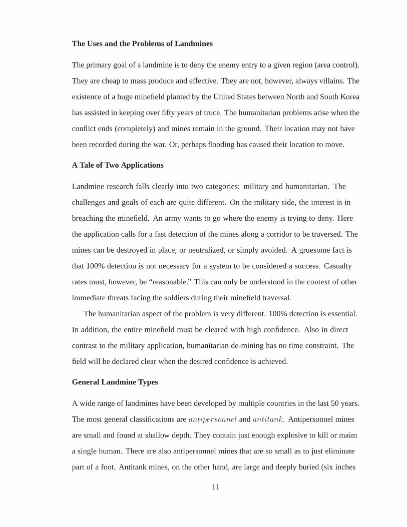
all the pixels in a vertical column. Figure 3.15 shows that this technique applied to the

31

Figure 3.12: Italian VS1.6 Landmine at 6” Depth

Figure 3.13: The HFT Applied to Every Point of the Image

32

Figure 3.14: The 20% Brightest Pixels of the Transformed Data

HFT image shows a strong indication of an object at the location of the VS1.6.

3.2.5 Pseudo Imaging Conclusions

A novel way of processing GPR signatures has been introducedcalled the Hyperbola

Flattening Transform. The algorithm utilizes the mathematics of conic sections to

transform the hyperbola into a line. The line can then be exploited using the Radon

Transform to produce a feature value for use in discrimination of false-alarms and

detection of low signal-to-noise ratio objects. This feature value can be thought of as a

summation of all the energy contained in the hyperbolic signature. After applying the HFT

to a VS1.6 buried at 6”, encouraging results were obtained. This is a plastic mine and is

buried deeply. The transformed data showed an enhancement of the landmine’s signal

while diminishing other signals caused by the stratified earth [31].

33

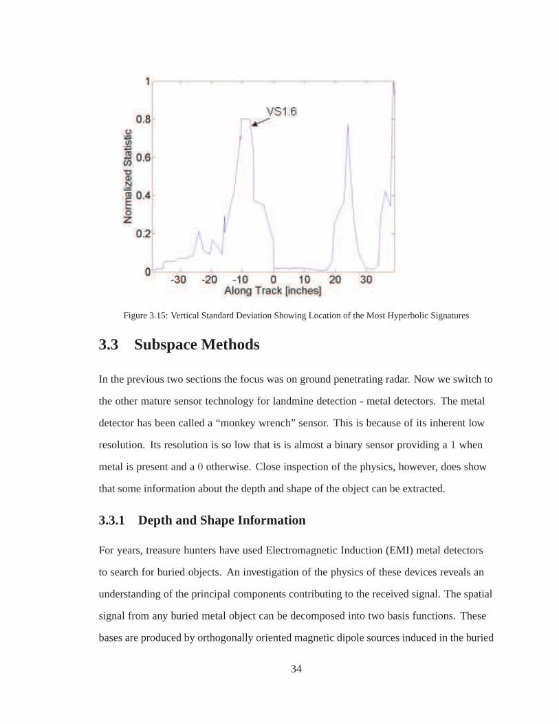
Figure 3.15: Vertical Standard Deviation Showing Locationof the Most Hyperbolic Signatures

3.3 Subspace Methods

In the previous two sections the focus was on ground penetrating radar. Now we switch to

the other mature sensor technology for landmine detection -metal detectors. The metal

detector has been called a “monkey wrench” sensor. This is because of its inherent low

resolution. Its resolution is so low that is is almost a binary sensor providing a1 when

metal is present and a0 otherwise. Close inspection of the physics, however, does show

that some information about the depth and shape of the objectcan be extracted.

3.3.1 Depth and Shape Information

For years, treasure hunters have used Electromagnetic Induction (EMI) metal detectors

to search for buried objects. An investigation of the physics of these devices reveals an

understanding of the principal components contributing tothe received signal. The spatial

signal from any buried metal object can be decomposed into two basis functions. These

bases are produced by orthogonally oriented magnetic dipole sources induced in the buried

34

object. Because of their characteristic appearance, the twobases have been called theΛ

andW basis functions. Since the induced sources behave like point sources, theΛ andW

basis functions are the same for all objects at the same depth. The object’s shape and metal

content determines the weighting ofΛ andW , which sum to produce the spatial signal

received by the metal detector.

The fact that all objects at the same depth can be representedas the summation of

two basis functions implies that the signal exists in a two dimensional vector subspace.

Identification of the subspace reveals the depth of the object. Once depth is known, the

basic shape of the object can be determined by the signal components. The metal content

(i.e., conductivity) and object size can be estimated by thecomponents’ magnitude.

Two applications of this signal representation are explored. First, a projection method

is used to estimate object depth. This method utilizes a projection matrix that projects

a normalized signal into the subspace of a ”shallow”, ”mid-depth”, and ”deep” object.

After the projection is made, thel2 norm of the sampled signal is computed. This norm is

a measure of the energy of the signal that ”survived” the projection. In a world without

noise, the subspace corresponding to true depth will not reduce the signal energy at all.

100% of the input signal energy will be found in the projectedsignal. When noise is

present, the true depth will still be revealed by the projector that rejects the least amount

of energy. (That is, only the energy contained in the additive noise will be rejected.)

The second application involves determining the object’s shape through estimation

of the object’s directional polarizability. Accurate estimation of polarizability requires

knowledge of the object’s depth. In other words, it is necessary to know the correct

signal subspace within which to make the estimates. (The depth could be provided by the

proposed projection algorithm just mentioned or through the use of an alternative sensor

like a ground penetrating radar.) Once depth is known, the object shape is identified by

estimating the polarizability of the object in the horizontal and vertical directions.

Computer simulations are used to test the two applications. Signals corresponding to

35

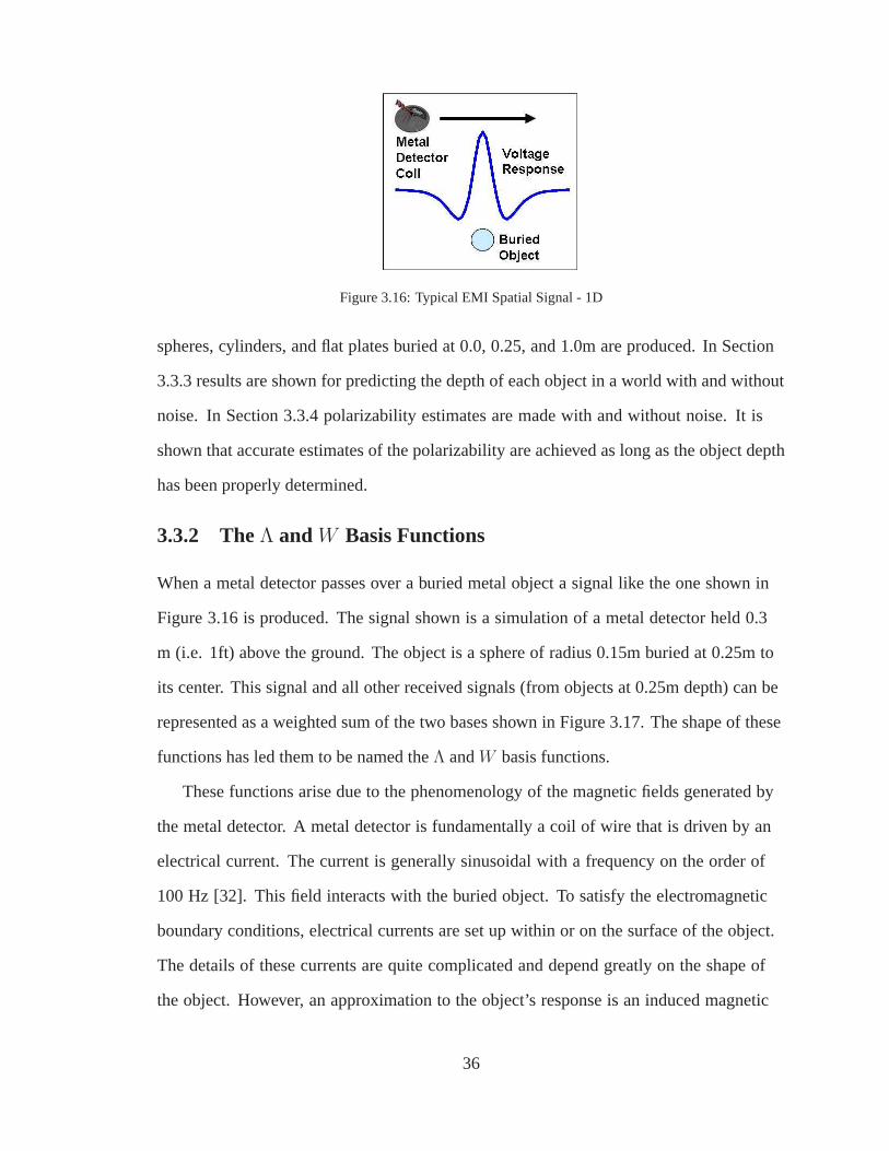
Figure 3.16: Typical EMI Spatial Signal - 1D

spheres, cylinders, and flat plates buried at 0.0, 0.25, and 1.0m are produced. In Section

3.3.3 results are shown for predicting the depth of each object in a world with and without

noise. In Section 3.3.4 polarizability estimates are made with and without noise. It is

shown that accurate estimates of the polarizability are achieved as long as the object depth

has been properly determined.

3.3.2 TheΛ and W Basis Functions

When a metal detector passes over a buried metal object a signal like the one shown in

Figure 3.16 is produced. The signal shown is a simulation of ametal detector held 0.3

m (i.e. 1ft) above the ground. The object is a sphere of radius0.15m buried at 0.25m to

its center. This signal and all other received signals (fromobjects at 0.25m depth) can be

represented as a weighted sum of the two bases shown in Figure3.17. The shape of these

functions has led them to be named theΛ andW basis functions.

These functions arise due to the phenomenology of the magnetic fields generated by

the metal detector. A metal detector is fundamentally a coilof wire that is driven by an

electrical current. The current is generally sinusoidal with a frequency on the order of

100 Hz [32]. This field interacts with the buried object. To satisfy the electromagnetic

boundary conditions, electrical currents are set up withinor on the surface of the object.

The details of these currents are quite complicated and depend greatly on the shape of

the object. However, an approximation to the object’s response is an induced magnetic

36

Figure 3.17: TheΛ andW Basis Functions

dipole [33]. Because higher order effects in magnetics have avery fast spatial decay rate,

the contribution of the more complicated physics is not observed by the metal detector. As

far as the metal detector is concerned, the buried object is just a magnetic dipole source.

This source will have components in both the vertical and horizontal directions. The

magnitudes of these dipoles change as the sensor passes overhead. TheΛ andW basis

functions take into account these changes. The weightings of the two bases come from the

polarizability of the object.

That is, the tendency of the object to allow a magnetic dipoleto exist in the vertical

and horizontal directions. The polarizability values are always constant no matter where

the sensor is located with respect to the buried object. Thisimplies that the polarizability

can be estimated and used as a rough measure of object shape.

s(x) = aΛd(x) + bWd(x) (3.14)

The shape of the buried object affects its polarizability. For instance, a sphere has no

inherent directionality. So, the polarizability is equal in all directions. A flat plate, on

the other hand, will allow the swirling currents induced by the sensor to exist on its flat

surface. If that surface is parallel to the earth’s surface,then there will be a large vertical

dipole response. The area of the flat plate perpendicular to the horizontal is very small. It

does not allow much current to flow so the horizontal polarizability of the plate is quite

small. (See Section 3.3.4 for more discussion.)

37

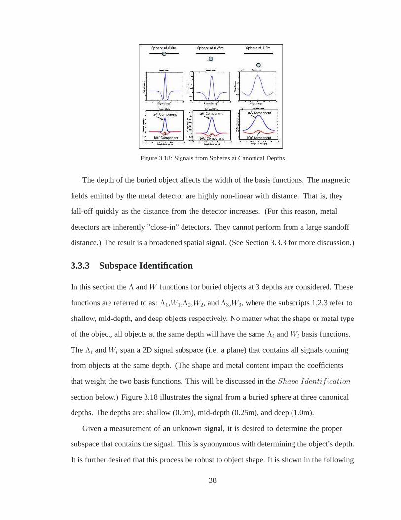
Figure 3.18: Signals from Spheres at Canonical Depths

The depth of the buried object affects the width of the basis functions. The magnetic

fields emitted by the metal detector are highly non-linear with distance. That is, they

fall-off quickly as the distance from the detector increases. (For this reason, metal

detectors are inherently ”close-in” detectors. They cannot perform from a large standoff

distance.) The result is a broadened spatial signal. (See Section 3.3.3 for more discussion.)

3.3.3 Subspace Identification

In this section theΛ andW functions for buried objects at 3 depths are considered. These

functions are referred to as:Λ1,W1,Λ2,W2, andΛ3,W3, where the subscripts 1,2,3 refer to

shallow, mid-depth, and deep objects respectively. No matter what the shape or metal type

of the object, all objects at the same depth will have the sameΛi andWi basis functions.

TheΛi andWi span a 2D signal subspace (i.e. a plane) that contains all signals coming

from objects at the same depth. (The shape and metal content impact the coefficients

that weight the two basis functions. This will be discussed in theShape Identification

section below.) Figure 3.18 illustrates the signal from a buried sphere at three canonical

depths. The depths are: shallow (0.0m), mid-depth (0.25m),and deep (1.0m).

Given a measurement of an unknown signal, it is desired to determine the proper

subspace that contains the signal. This is synonymous with determining the object’s depth.

It is further desired that this process be robust to object shape. It is shown in the following

38

paragraphs that the subspace from a sphere, a cylinder, and aflat plate buried at 0.0, 0.25,

and 1.0m depths can be identified by projecting each signal into the shallow, mid, and deep

subspaces and choosing the subspace that rejects the least amount of signal energy. This

approach works even in the presence of noise.

The subspace projection method is used here to identify object depth. Equations 3.16,

3.17, and 3.18 defines a set of matrices called projection matrices [34]. When a projection

matrix operates on an observed signal, it has the effect of revealing the signal components

found in that subspace. This fact is often used to reduce noise is signals. In this application

a mismatched subspace will have the effect of reducing the energy of the signal. The

projection matrices for the subspaces are formed accordingto Equations 3.16, 3.17, and

3.18. HereΛd andWd in Equation 3.15 represent column vectors formed by digitally

sampling the basis functions.

Hd = [ Λd Wd ] (3.15)

Pshallow = H1(HT1 H1)

−1HT1 (3.16)

Pmid = H2(HT2 H2)

−1HT2 (3.17)

Pdeep = H3(HT3 H3)

−1HT3 (3.18)

Unfortunately, the subspaces occupied by objects at different depths are not orthogonal.

They can be geometrically be interpreted as slanted planes.Some energy from signals at,

say, 0.0m will be present in the subspace occupied by a signalat 1.0m. Table 3.2 shows

39

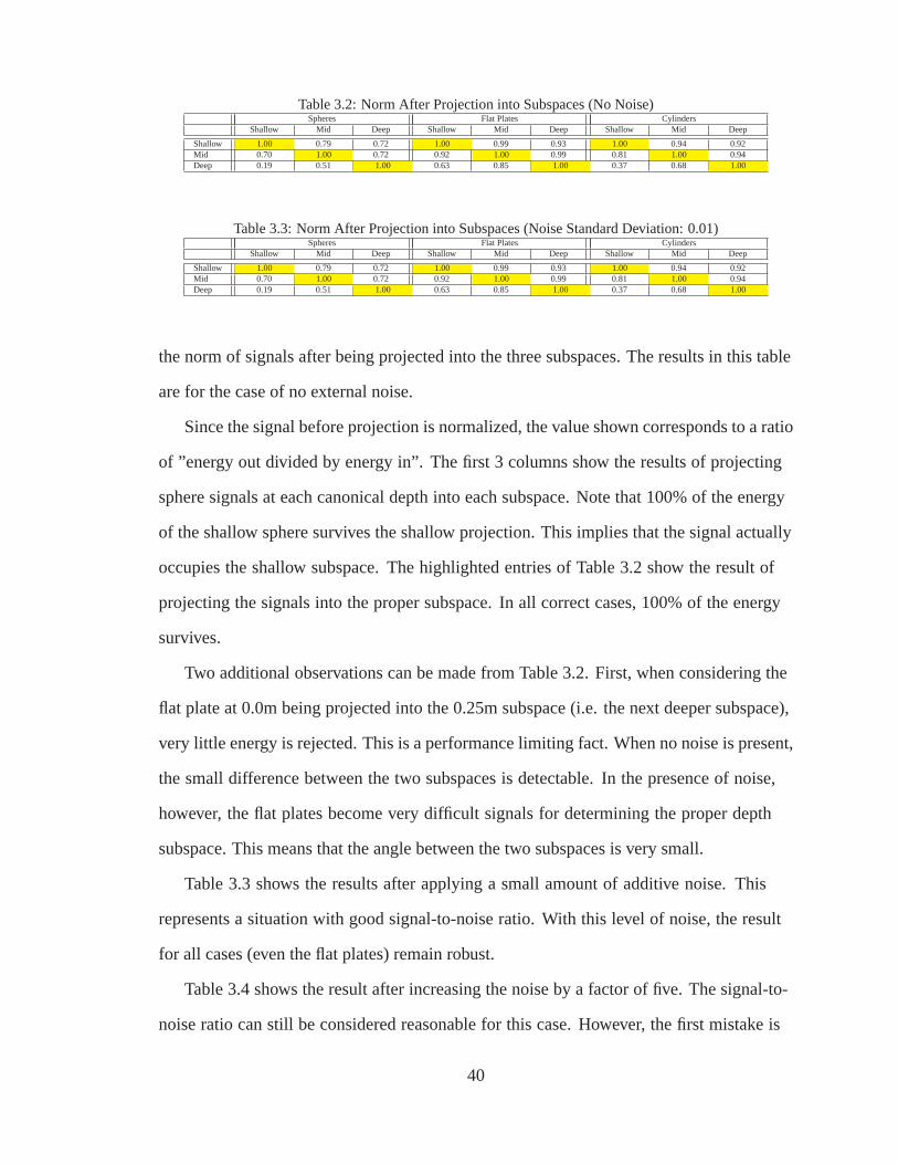
Table 3.2: Norm After Projection into Subspaces (No Noise)Spheres Flat Plates Cylinders

Shallow Mid Deep Shallow Mid Deep Shallow Mid Deep

Shallow 1.00 0.79 0.72 1.00 0.99 0.93 1.00 0.94 0.92Mid 0.70 1.00 0.72 0.92 1.00 0.99 0.81 1.00 0.94Deep 0.19 0.51 1.00 0.63 0.85 1.00 0.37 0.68 1.00

Table 3.3: Norm After Projection into Subspaces (Noise Standard Deviation: 0.01)Spheres Flat Plates Cylinders

Shallow Mid Deep Shallow Mid Deep Shallow Mid Deep

Shallow 1.00 0.79 0.72 1.00 0.99 0.93 1.00 0.94 0.92Mid 0.70 1.00 0.72 0.92 1.00 0.99 0.81 1.00 0.94Deep 0.19 0.51 1.00 0.63 0.85 1.00 0.37 0.68 1.00

the norm of signals after being projected into the three subspaces. The results in this table

are for the case of no external noise.

Since the signal before projection is normalized, the valueshown corresponds to a ratio

of ”energy out divided by energy in”. The first 3 columns show the results of projecting

sphere signals at each canonical depth into each subspace. Note that 100% of the energy

of the shallow sphere survives the shallow projection. Thisimplies that the signal actually

occupies the shallow subspace. The highlighted entries of Table 3.2 show the result of

projecting the signals into the proper subspace. In all correct cases, 100% of the energy

survives.

Two additional observations can be made from Table 3.2. First, when considering the

flat plate at 0.0m being projected into the 0.25m subspace (i.e. the next deeper subspace),

very little energy is rejected. This is a performance limiting fact. When no noise is present,

the small difference between the two subspaces is detectable. In the presence of noise,

however, the flat plates become very difficult signals for determining the proper depth

subspace. This means that the angle between the two subspaces is very small.

Table 3.3 shows the results after applying a small amount of additive noise. This

represents a situation with good signal-to-noise ratio. With this level of noise, the result

for all cases (even the flat plates) remain robust.

Table 3.4 shows the result after increasing the noise by a factor of five. The signal-to-

noise ratio can still be considered reasonable for this case. However, the first mistake is

40

Table 3.4: Norm After Projection into Subspaces (Noise Standard Deviation: 0.05)Spheres Flat Plates Cylinders

Shallow Mid Deep Shallow Mid Deep Shallow Mid Deep

Shallow 0.96 0.75 0.65 0.95 0.94 0.91 0.92 0.89 0.85Mid 0.68 0.97 0.64 0.90 0.94 0.95 0.77 0.94 0.86Deep 0.16 0.51 0.93 0.63 0.84 0.95 0.30 0.61 0.94

Table 3.5: Norm After Projection into Subspaces (Noise Standard Deviation: 0.3)Spheres Flat Plates Cylinders

Shallow Mid Deep Shallow Mid Deep Shallow Mid Deep

Shallow 0.52 0.32 0.42 0.31 0.38 0.19 0.42 0.44 0.48Mid 0.37 0.62 0.48 0.31 0.37 0.26 0.31 0.43 0.52Deep 0.18 0.37 0.62 0.36 0.33 0.30 0.20 0.33 0.52

made here by the algorithm for the flat plate case. This limiting condition can be explained

by considering theW basis function for the flat plate. Due to the thin nature of theflat

plate, there is very little polarizability in the horizontal direction. TheW basis function is,

therefore, almost non-existent. Loss of theW basis function makes determining depth for

this class of object virtually impossible when significant noise is present.

Objects other than flat plates show much better robustness tonoise. Table 3.5 shows a

30dB increase in noise. The resulting projections show thatthe depth of flat plates and the

cylinders can no longer be determined with any confidence. The spheres, however, still

give correct depth estimates.

3.3.4 Shape Identification

Once object depth is determined the object polarizability can be estimated. Figure 3.19

shows the signal components for 3 canonical shapes: a sphere, a cylinder, and a flat plate.

The polarizability of each shape type is known.

For the sphere the polarizability is:Pz = 1.0, Px = 1.0. For cylinders:Pz = 1.0,

Px = 0.5. And for flat plates:Pz = 1.0, Px = 0.2. This is summarized in Table 3.6.

These values were chosen for the simulation intuitively. The sphere should not have a

bias in any direction because it is spherical. (This is a minor assumption that may not be

true in reality due to the ”infinite conducting half-space”,i.e. the ground, within which the

41

Figure 3.19: Canonical Objects at Same Depth

Table 3.6: Shape PolarizabilitiesPz Px

Sphere 1.0 1.0Cylinder 1.0 0.5Flat Plate 1.0 0.2

object is buried.) The flat plate, on the other hand, has a large area perpendicular to the

vertical magnetic field. The swirling eddy currents inducedby the sensor result in a large

vertical polarizability. Because the flat plate is thin, it has only a little area perpendicular

to the horizontal magnetic field. The resulting polarizability is small. Similarly, in the case

of the cylinder, if it is ”short”, then it will have less ”height” than it has ”diameter”. By the

same line of thinking it is expected that the horizontal direction will be less polarizable

than the vertical.

The minimum squared error inversion algorithm for estimating polarizability is shown

in Equation 4 [35].

pz

px

=(

HT

dHd

)−1HT

ds (3.19)

In this equationd is an estimate of the object depth, andHd is defined by Equation

3.15. The vectors represents a column vector containing the sampled spatial signal. Table

42

Table 3.7: Polarizability Estimates (No Noise)Shallow Mid Deep Shallow Mid Deep Shallow Mid Deep

Shallow Pz 1.00 0.93 0.45 1.00 0.76 0.38 1.00 0.82 0.41Px 1.00 0.41 -0.42 0.20 -0.27 -0.62 0.50 -0.01 -0.54

Mid Pz 0.53 1.00 0.78 0.96 1.00 0.63 0.80 1.00 0.69Px 0.82 1.00 0.09 0.41 0.20 -0.44 0.56 0.50 -0.24

Deep Pz -0.10 0.30 1.00 0.67 0.89 1.00 0.38 0.67 1.00Px 0.13 0.59 1.00 0.33 0.43 0.20 0.26 0.49 0.50

Table 3.8: Polarizability Estimates (Noise Var: 0.01)Shallow Mid Deep Shallow Mid Deep Shallow Mid Deep

Shallow Pz 1.00 0.92 0.46 0.98 0.75 0.38 1.01 0.84 0.38Px 1.00 0.40 -0.40 0.18 -0.26 -0.61 0.52 0.00 -0.55

Mid Pz 0.53 0.99 0.79 0.96 0.98 0.62 0.80 1.02 0.67Px 0.82 1.00 0.10 0.40 0.18 -0.44 0.58 0.52 -0.25

Deep Pz -0.11 0.29 0.99 0.68 0.89 1.00 0.36 0.67 0.99Px 0.12 0.58 1.00 0.34 0.41 0.20 0.25 0.50 0.48

3.7 illustrates the results of using proper and mismatchedHd matrices. In the case where

the properH (i.e. the proper basis set) is used, the computed polarizability is exact. For

example, the sphere at any depth is shown to be properly estimated with unit polarizability

in the vertical and horizontal directions. The same is true for the flat plates and the

cylinders. Use of a mismatched bases, however, results in extremely misleading estimates.

In the case of additive noise contaminating the signal, a similar result is observed.

Table 3.8 contains a small amount of additive noise. All canonical objects, however, are

estimated with little error. Increasing the noise in the observations, increases the error in

the final estimates.

Table 3.9 shows the effect of higher noise. Looking at the subspace identification

results of Section 3.3.3, it is clear that the depth estimation algorithm will fail before the

polarizability estimator of Section 3.3.4. If the depth is determined using another sensor,

the polarizability estimator will be able to classify objects by their shape even in the

presence of significant noise.

3.3.5 Subspace Method Conclusions

Two basis functions have been presented that form a basis formetal detector signals.

These functions are theΛ andW basis functions. It has been shown that objects from the

43

Table 3.9: Polarizability Estimates (Noise Var: 0.05)Shallow Mid Deep Shallow Mid Deep Shallow Mid Deep

Shallow Pz 1.06 0.95 0.42 0.97 0.71 0.38 0.99 0.84 0.40Px 1.12 0.37 -0.40 0.23 -0.33 -0.66 0.49 0.02 -0.53

Mid Pz 0.52 1.05 0.75 0.89 0.96 0.61 0.84 1.00 0.67Px 0.87 1.00 0.09 0.37 0.12 -0.53 0.64 0.53 -0.23

Deep Pz -0.17 0.33 0.97 0.63 0.89 1.07 0.36 0.65 0.96Px 0.08 0.58 1.00 0.28 0.36 0.22 0.31 0.50 0.47

same depth have the same basis functions regardless of shapeand metal content. Object

size and metal content affect the weightings of the two basisfunctions. Object depth, on

the other hand, affects the width of the functions.

A subspace projection method was introduced that identifiedthe proper basis of a

measured signal from an object at unknown depth. The method was shown to work

perfectly in a low noise environment. When noise is added, however, the similarity

between subspaces made depth determination difficult. Thiswas especially true of the flat

plate object.

Once object depth was determined (or if it was provided from another sensor), the

object shape was determined by estimating the polarizability of the of the object in the

vertical and horizontal directions. Objects that are significantly different, like the sphere,

cylinder, and flat plate, are easy to identify even in the presence of significant noise.

A mismatch in depth estimation, however, was shown to cause significant error in the

estimated polarizability values.

This work has shown how the physics of the magnetic field produced by a metal

detector can be used to identify a signal basis set. This basis is composed of two principal

functions with which all metal detector signals can be represented. A careful use of

the these bases can be made to reveal both the depth of the object and its basic shape.

Future research will expand the analysis to scanning two spatial dimensions, as well as,

considering buried object response to multiple frequencies.

44

CHAPTER IV

STATISTICAL APPROACHES

4.1 Multimodal Detection

Landmine detection often employs multiple sensors due to the diversity of sensor

signatures encountered. Two commonly used sensors are ground penetrating radar (GPR)

and electromagnetic induction (EMI) metal detectors. Both sensor technologies have been

proven to be very effective in detecting metal landmines. The GPR has been shown to

detect non-metal mines because radar signals are reflected by the dielectric discontinuity

between the soil and the plastic mine casings. Also, in some cases the EMI has been

used to detect non-metal cased mines by detecting the small amount of metal contained

in the mine’s firing pin. Theoretically, therefore, both sensors are capable of detecting all

landmine types. In practice, however, performance of each sensor is challenged by low

signal-to-noise ratios on some landmines depending on typeof mine, burial depth, and

environmental conditions.

In this work two environments are considered. The first is a clay background and

the second is gravel. These two backgrounds offer a look at how EMI and GPR sensor

statistics change based on the environment surrounding thelandmine.

4.1.1 Multimodal Landmine Detection

Multi-modal sensor systems describe a single sensor that utilizes separate sensor modes

or a collection of sensors that employ different physical phenomenology. By utilizing

multiple modes, a greater diversity of information is obtained. In this work we look at

45

Figure 4.1: Estimated Joint Probability Density Functions

a vehicle mounted landmine detection system using an array of EMI and GPR sensors.

The two sensor arrays each raster scan an image of the ground response as the vehicle

moves forward. The two images are registered at the pixel-to-pixel level for detection of

landmines.

Joint Probability Densities

A set of training data is used to establish a 2D joint probability density between the

pixels of the EMI image and the pixels of the GPR image. Six classes of landmines are

considered. The classes are arranged according to depth forboth metal cased and plastic

cased mines. The landmine classes are: 1) deeply buried metal cased 2) mid-depth metal

cased 3) shallow depth metal cased 4) deeply buried plastic cased 5) mid-depth plastic

cased and 6) shallow plastic cased. All classes are for anti-tank mines. A seventh class is

designated background.

Figure 4.1 shows the estimated joint probability densitiesfor background pixels and

metal cased landmines. These PDFs were generated by extracting pixels of each class

from EMI and GPR training images. The sample mean, variance,and correlation were

then computed, and the PDFs generated using a bivariate Gaussian model. These PDFs

will be used to generate the posterior probabilities described in Section 4.1.1.

46

Figure 4.2: Marginalized Probability Density Functions ofMid-depth, Metal Cased Landmines

Single Mode (Marginalized) Densities

Single-mode approaches for the MAP detector exist for both the GPR and EMI sensors.

The 2D PDFs are marginalized to only include the statistics of one sensor. This is done by

”integrating out” one of the sensors. The MAP approach described in Section 4.1.1 can

be used in the multi-modal approach or in single mode with either sensor. Section 4.1.3

shows the performance advantage of utilizing the multi-modal approach.

Maximum A Posteriori Detection

In this application we have seven classes of objects. The sensors respond to each object

class in a different way. This difference manifests itself statistically in the resulting

observations as a change in the probability distributions of the observed pixels. For

example, the amplitudes of the received signals for both sensors are greatly affected by

the distance from the sensor to the object. This results in very different pixel probabilities

between landmines buried shallow and landmines buried deep. This can be seen in Figure

4.1 where the mean and variance of the deep, mid-depth, and shallow landmines have

significantly different values. The idea behind the MAP detector is to make a measurement

and use that observation to determine which probability distribution is the likeliest to have

produced that observed value. For this application, all classes have signatures that occupy

more than 1 pixel. This fact can be used in the MAP processor byperforming multiple

measurements on the same object as it passes beneath the vehicle.

The Maximum A Posteriori (MAP) detection approach proposedhere takesN

47

Figure 4.3: Signatures from a Mid-depth, Metal Cased Landmine

looks at an object sequentially as the object passes by the sensor. Before beginning the

measurements, an a priori probability is assigned to the classes. Since there are seven

classes, the a priori probability is set to17

for each class. After each measurement Bayes

Rule is used to update the probability assignments. Equation4.1 is called the Update

Equation. For the first measurement it translates the prior probability assignment to a

posterior probability. Likewise, for all subsequent observations it continues to update the

probabilities as new measurements are made.P (y|x) in Equation 4.1 is the observation

model for a given classx. The probabilitypn(x) is the probability that an observed object

is classx for thenth observation,yn.

pn(x) =p(yn|x)pn−1(x)∑

p(x, yn)(4.1)

4.1.2 Adapting to the Environment

The probability distributions shown in Figures 4.1 and 4.2 are for landmines in a clay

background environment. If this environment were changed,it would be reflected in a

new set of distributions. Figure 4.4 illustrates the tremendous variability that can be seen

between observations made in a clay background and observations in a gravel background.

The gravel lane shows a significantly higher amount of attenuation than the clay lane. This

is likely due to the amount of moisture that is held within thematerial. Clearly there is a

need for the sensor to adapt to this change in class statistics.

48

Figure 4.4: PDFs of EMI and GPR pixels from mid-depth buried metal landmines. (left) Lane material isclay. (right) Lane material is gravel.

One way to assist in adapting the sensor statistics is the useof electromagnetic models

coupled with measurements of the environmental parameters. A GPR measurement of

the ground dielectric permittivity can be made by looking atthe ground bounce return.

Mapping the reflection coefficient into dielectric permittivity for a homogeneous ground

follows Equation 4.3 [36].

R12 =1 − 1√

ǫr

1 + 1√ǫr

(4.2)

Figure 4.5 shows the inverse mapping. Wet ground representsa relative permittivity in

the range of 40 to 60. Dry ground represents a relative permittivity from 3 to 10. It can

be shown that an estimate for dry ground is somewhat robust tonoise in the observation.

In other words, a few observations of the ground bounce return can be averaged to very

effectively estimate the permittivity value. Once this value has been obtained, the statistics

of the seven classes can be estimated based on a simple electromagnetic scattering model.

When the ground is wet, however, the estimation process is more complicated. A small

amount of noise in the reflection coefficient could double theestimated permittivity value.

This means that many observations will need to be averaged toproduce a robust estimate.

However, once a robust estimate is obtained, simple scattering models can be use to

generate the class probabilities.

49

Figure 4.5: Inverse Mapping from Reflection Coefficient to Dielectric Permittivity

4.1.3 Detection Performance

In this section the results of applying the sequential MAP detector to multi-modal and

single mode landmine data are shown. For each case 5 observations are made on each

object as it passes the sensor arrays. The results show that multi-modal processing

outperforms single mode.

Here it is also shown that adapting to the environment is an important part of optimal

performance. The multimodal MAP detector is re-trained forapplication to a wider set of

environmental conditions. In this case the conditions include a clay soil background and

a gravel background. Training for both environments simultaneously means widening the

class statistics to handle measurements that are more variable. The consequences of this

generalization are a significant reduction in detector performance.

Multimodal Versus Single Mode

Here the MAP detector described above is applied in both multi-modal and single sensor

modes. In single sensor mode the EMI and GPR sensors apply thetrained 1D PDF 5 times

as the objects are encountered. The EMI initially has the better performance because it is

very good at detecting metal cased landmines. Eventually, however, the GPR reaches the

maximum detectible number of objects before the EMI becauseit is able to better handle

50

Figure 4.6: Multi-modal Versus Single Mode MAP Detection Algorithms - Multi-modal processing has aclear advantage.

the plastic cased mines.

The multi-modal detector has the advantage of utilizing theEMI’s ability to detect

metal and the GPR’s ability to detect plastic. Also, it has another significant advantage.

The background clutter shown in the Left Frame of Figure 4.1 appears to have a bifurcated

nature. That is there appear to be some clutter objects in thebackground that a observed

by the EMI and not the GPR while others are observed by the GPR and not the EMI. The

EMI may be seeing metal or metal residue from very small metallic clutter objects. These

objects have too small of a radar cross section to appear in the GPR data. The GPR, on

the other hand, is observing rocks or other dielectric discontinuities that are not observable

by the EMI. This nature of the background noise allows for a powerful discrimination in

the 2D PDFs. This is due to the correlation that exists between the EMI and GPR sensors

when observing landmine signatures.

Performance With and Without Adapting

The importance of adapting to environmental changes cannotbe stressed enough. Soil that

is wet will produce very different sensor statistics than soil that is dry. In this section we

illustrate the need for adaptation when the soil environment changes. The two lanes consist

of the clay and gravel lanes described in Section 4.1.2. In Section 4.1.2 it was observed

51

Figure 4.7: Multi-modal MAP Detector Trained and Applied toClay Background Compared to aGeneralized Detector Trained and Applied to Clay and GravelBackgrounds

that the mid-depth landmine statistics show much greater attenuation in the gravel lane

than in the clay. This could be an indication of moisture being present in the gravel lane.

Moisture causes the dielectric permittivity and the conductivity of the soil to increase as

much as an order of magnitude. Since attenuation of electromagnetic energy is directly

determined by the permittivity and conductivity of the soil, the statistics of the signatures

found in the collected imagery change.

For the combined training of the MAP detector, a set of lanes was sequestered from

both the clay and gravel backgrounds. The 2D PDFs were determined and applied to the

remaining lanes of both backgrounds. The result is a detector that is generalized to handle

both backgrounds. Unfortunately, the performance of the detector is reduced significantly.

4.1.4 Multimodal Summary

In this work a maximum a posteriori (MAP) detection algorithm is developed that

utilizes sensor statistics to classify metal and plastic cased landmines. The MAP sensor

can be applied multi-modally using a 2D PDF trained from signatures produced by an

electromagnetic induction (EMI) metal detector and a ground penetrating radar (GPR). It

can also be applied to either sensor in a single sensor mode. Application to experimental

data shows that the multi-modal approach significantly outperforms either sensor run in

52

single sensor mode. The data was obtained from a clay background mine lane.

A second experiment shows that the statistics of the sensor can change significantly

between the clay background lane and a gravel background lane. The second experiment

trains the MAP detector for both environments. This makes the detector more general but

the end results is a for less powerful detection performance. Adapting the trained statistics

when background changes occur is an essential part of optimized system performance.

Future work in the area of adaptive algorithms will include the employment of physical

models for assisting the prediction of sensor statistics. Also, the MAP detector will be

expanded to take advantage of the spatial signatures observed from the landmines in

two and three dimensions. This work considered only landmine classes. In a real world

environment, clutter classes from metal and/or non-metal objects lying on the surface will

also be taken into account. An approach for scheduling additional sensor measurements

to discriminate target and clutter types is proposed in [37]. And, finally, future work will

include non-myopic approach that will account for the time required to make certain

sensor measurements. This approach will choose sensors appropriately to minimize the

amount of time required to traverse a specified distance. [38] [39] [40] [41]

4.2 Bayes Networks

A Bayesian Network is a way of thinking about joint probabilities. It allows for an

associated PDF to be broken down into a system of conditionaldependencies [42]. Using

Bayes rule a joint PDF can be rewritten as a product of conditional probabilities. The

attraction of this is that the conditional probabilities may be easier to train than the full

joint PDF.

In [42] a burglar alarm problem is considered. The event of the alarm going off is a

binary random variable,Z. The alarm can be set off by a burglar or by an earthquake

(the problem takes place in southern California). Two neighbors have been asked to call

the owner at work when the alarm goes off. Probabilities of calling are given for each

53

Figure 4.8: A Bayesian Network Structure for the Burglar Alarm Problem

neighbor. The events of the neighbors calling are,Y1, Y2. The root event,X, is a random

variable taking on the value0 for an earthquake,1 for a break in, and2 for no alarm (the

neighbors are calling for some other reason). The joint probability of all these events can

be modelled as:

P (Y1, Y2, Z,X) = P (Y1|Z)P (Y2|Z)P (Z|X)P (X) (4.3)

The conditional probabilities and their relationship can be graphically displayed in an

acyclic directed graph. For the burglar alarm problem, this looks like Figure 4.8. The

variableX here is called the parent ofZ. Z, meanwhile, is the parent ofY1 andY2. The

layer of the network inhabited byY1 andY2 is called the observation layer.Z, on the other

hand, is in thehidden node layer. The term hidden nodes implies that we (here the owner)

does not directly observe the alarm going off. The goal is to use probabilistic reasoning to

decide whether the alarm is due to a burlary or due to an earthquake. This decision is to be

made based on the observations.

We wish to apply this technique to the landmine detection/classification problem.

In this case, the event is the existence of a landmine. The alarm event could be an

anti-personnel, anti-tank, a false alarm, or any number of acollection of non-mine objects.

54

Figure 4.9: A Bayesian Network Structure for the Landmine Problem

The hidden nodes could be associated with soil types, objectdepths, and object metal

content. (Plastic mines have low metal content while metal cased mines have high.) A

possible network structure for this problem is shown in Figure 4.9.

55

CHAPTER V

SENSOR SCHEDULING

5.1 Single Confirmation Sensor - Active Sensing

Active Sensing is a popular form of sensor scheduling that utilizes a measure of increased

certainty called information gain to dynamically choose a sensor to apply to a given

decision problem [43]. In this section a basic application of the concepts of Active Sensing

are applied in the area of landmine detection. Active sensing is a way of scheduling

multiple sensors, which have diverse capabilities and uses. Each sensor is considered a

resource and a statistical model of how objects of interest react to each sensor is known.

As a sensor system begins interrogating an area for objects it decides dynamically which

sensor to use to provide the maximum amount of information.

The architecture proposed in this work uses traditional vehicle mounted scanning

sensors (EMI and GPR arrays) to assign prior probabilities to all locations in the mine

lane. This information is given to the ”Sensor Management Decision Engine”, which

applies Active Sensing to decide the most powerful confirmation sensor to deploy. In the

myopic case, a sensor is always deployed to interrogate every 1ft by 1ft square of the mine

lane. The time sensitive case, however, sometimes chooses not to deploy a sensor.

Myopic sensor management algorithms consider only the immediate situation when

determining what action to schedule [44]. (Webster’s Dictionary defines myopic as,

”Lacking long-range perspective in thinking or planning.”) Non-myopic approaches

consider other information concerning the situation or theenvironment that can impact

56

Figure 5.1: Proposed Architecture for Applying Sensor Management to a Vehicle Mounted LandmineDetection System

the performance of the system [45]. All sensors do not perform their measurements in the

same amount of time. By taking time into account, the platformcan traverse the given

territory in the minimum amount of elapsed time. In the example situation presented

here, the myopic only approach traversed the mine lane in 270minutes. By accounting

for processing time the approach traversed the lane in 25 minutes. Some degradation in

classification performance was incurred in the faster case.

Information gain is a quantity that describes the amount a sensor reduces the

uncertainty in information about an object. In a tracking application this implies knowing

the object’s location and velocity with greater accuracy. In the landmine area this implies

better knowledge of an object’s depth and/or type. In landmine detection some sensors are

capable of providing information about some objects and notothers. For example, a metal

detector can be used to provide information about metal content for metal cased mines.

This information can be used to eliminate false-alarms caused by metallic clutter on the

surface. It is less useful, however, to use the metal detector when interrogating a low-metal

object. In the case of the plastic cased landmine a metal detector may pick up a small

amount of metal in the firing-pin. However, this measurementis sometimes not available

due to small signal-to-noise ratio. The sensor system wouldlikely do better in this

situation by deploying a chemical detector (olfactory sensor) that could detect the presence

57

of TNT. Or it might be more useful to utilize the ground penetrating radar to determine if

the object is laying on the surface or buried. If the object ison the surface it may be most

useful to aim a visible light camera to investigate the object. The goal, therefore, is to

schedule sensors appropriately based on observations madeby the sensor platform. Active

Sensing is a method of realizing effective sensor scheduling by predicting the information

gain potential of available system resources. In this work aSensor Management Decision

Engine has been implemented in software that decides what confirmation sensor to deploy

(if at all) based on information provided by the scanning sensors.

5.1.1 Sensor Management using Active Sensing

Over the years many sensor technologies have been proposed and developed for detecting

landmines. A few of these include: ground penetrating radar, electromagnetic induction

metal detectors, magnetic quadrupole resonance, infra-red radiometers, visible light

cameras, passive magnetometers, olfactory sensors, and many more. Some sensors have

been useful as long-range scanning devices. These are technologies that can be used at

a large standoff distance. Examples of standoff sensors are: synthetic aperture radar,

infra-red radiometers, and passive millimeter wave radiometers. Other sensors can be

used for scanning, but are only effective at close distances. Examples of these close-in

sensors are: passive magnetometers and electromagnetic induction metal detectors. Other

technologies have been shown to be useful for scanning only small regions. These latter

sensors have become known as confirmation sensors.

The focus here is on the use of active sensing on a vehicle based detection system. The

starting point is an assumption that all classes of objects are equally likely. By employing

a scanning sensor an initial observation is made. Bayes rule is then used to update the

uniform priors. Equation 4.1 is known as the update equation.

Wherepn−1(x) represents the class probabilities for the state vector x for the previous

observation. The statistical modelp(y|x) is the knowledge of how the sensor measurement,

58

y, will respond statistically to the object state,x. The summation in the denominator is a

normalizing constant.

Once the scanning observation has been made, the sensor manager must decide what

confirmation sensor to deploy (or to not deploy one at all). Here the Renyi divergence is

used to predict the expected information gain for the available sensors [46].

D(pn||pn−1) =1

1 − αln

(∫

pαn(x)p1−α

n−1(x)dx

)

(5.1)

The probabilitiesPn are the expected probability distribution of the classes after the

next observation.Pn−1 is the probability distribution of the classes after the previous

observation. The divergence computation responds to the probabilities with a larger

divergence value if the variance in the second probability distribution has a lower variance

than the first. This means that ifPn is describing the class with more certainty, then the

sensor is more likely to be chosen and deployed. The sensor out of all the resources that

provides the greatest divergence (i.e. the greatest information gain) is deployed. Note that

theα parameter is a shape parameter that can be adjusted to optimize performance.

The classes that will be considered in this paper are: 1) deeply buried, metal cased

anti-tank mine, 2) mid-depth buried, metal cased anti-tankmine, 3) shallow buried, metal

cased anti-tank mine, 4) deeply buried, plastic cased anti-tank mine, 5) mid-depth buried,

plastic cased anti-tank mine, 6) shallow buried, plastic cased anti-tank mine, 7) aluminum

clutter on surface, 8) non-metal clutter on surface, 9) ironclutter on surface. The prior

distribution that will be applied to these classes is 0.1 (that is, a uniform prior.)

Active sensing can be employed at all levels of the landmine detection problem. If

standoff (i.e. airborne) sensors were used to identify a minefield, the information collected

by these sensors could be held on-line for assigning the prior probability distributions of

given regions. This implies a co-operative network of airborne and ground based vehicles

involved in the landmine detection process. Such a network could have the airborne

59

vehicles queuing ground based vehicles to specific locations or ground based vehicles

queuing stored airborne assets for confirmation [47].

5.1.2 Scanning Sensor Simulations

For the purpose of studying a realistic vehicle based landmine detection system, a system

with traditional scanning sensors and a suite of confirmation sensors is proposed. The

simulated scanning sensors will be used to acquire possiblelandmines and the confirmation

sensors will be used to show how the additional sensors are able to eliminate uncertainty

using Active Sensing. In this section the scanning sensor simulations are introduced.

These sensors are an array of electromagnetic induction metal detectors and an array of

ground penetrating radar.

Figure 5.2 shows a sample simulation of an EMI signature. This simulation was

generated using a point model of a magnetic dipole source (i.e. a current loop) over a

conducting half space [47]. The sample rate in the along track direction is 2” (5cm).

The sample rate in the cross track direction is 16” (40cm). The cross track sample rate

represents the distance between adjacent sensors mounted on the system.

The target in Figure 5.2 is an anti-tank landmine buried at 3”. (That is, 3” from the

earth surface to the top of the landmine.) The brightest partof the signature corresponds

to the sensor passing directly over the top of the mine. The dark regions surrounding the

center are negative voltage readings. This sign reversal iscaused by the incident magnetic

field of the metal detector coil. As the coil passes over the mine, the dipole nature of the

magnetic field reverses in direction. Some real world sensors handle this phenomenon in

different ways. Typically, an absolute value is taken by thereceiver. In this simulation we

have chosen to take the real part, which retains the sign reversal. The operating frequency

of this simulation was 75Hz.

The GPR produces a similar scanning signal. Figure 5.3 showsa 2D representation of

the GPR signature. This simulation was produced by simulating a stepped frequency radar

60

Figure 5.2: Simulated Signature of an EMI Scanning Sensor Array

Figure 5.3: Simulated Signature of a GPR Scanning Sensor Array

61

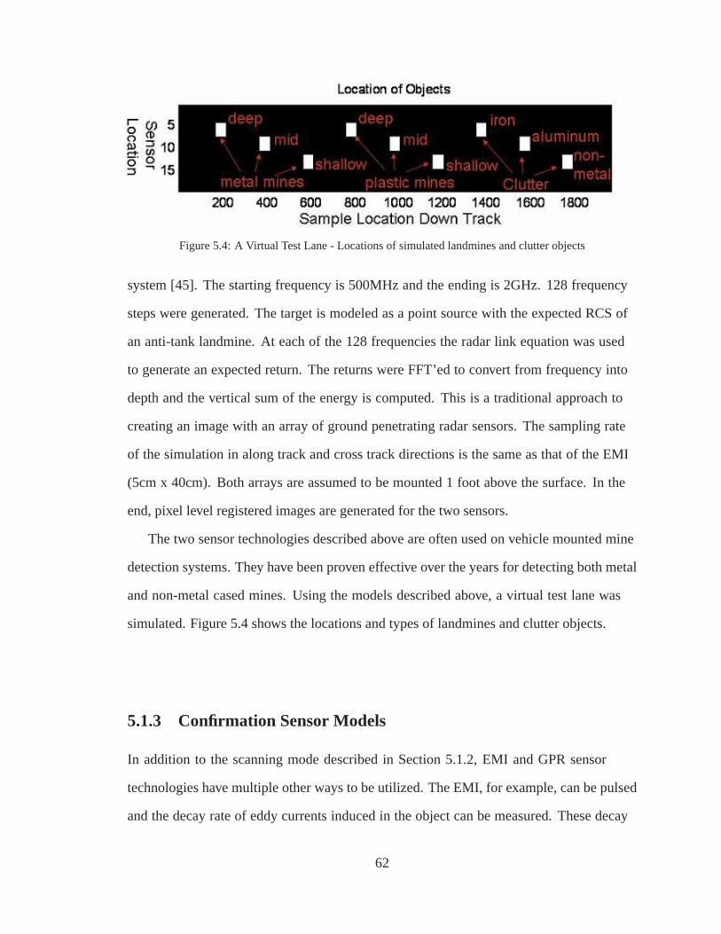
Figure 5.4: A Virtual Test Lane - Locations of simulated landmines and clutter objects

system [45]. The starting frequency is 500MHz and the endingis 2GHz. 128 frequency

steps were generated. The target is modeled as a point sourcewith the expected RCS of

an anti-tank landmine. At each of the 128 frequencies the radar link equation was used

to generate an expected return. The returns were FFT’ed to convert from frequency into

depth and the vertical sum of the energy is computed. This is atraditional approach to

creating an image with an array of ground penetrating radar sensors. The sampling rate

of the simulation in along track and cross track directions is the same as that of the EMI

(5cm x 40cm). Both arrays are assumed to be mounted 1 foot abovethe surface. In the

end, pixel level registered images are generated for the twosensors.

The two sensor technologies described above are often used on vehicle mounted mine

detection systems. They have been proven effective over theyears for detecting both metal

and non-metal cased mines. Using the models described above, a virtual test lane was

simulated. Figure 5.4 shows the locations and types of landmines and clutter objects.

5.1.3 Confirmation Sensor Models

In addition to the scanning mode described in Section 5.1.2,EMI and GPR sensor

technologies have multiple other ways to be utilized. The EMI, for example, can be pulsed

and the decay rate of eddy currents induced in the object can be measured. These decay

62

Table 5.1: Averages1 2 3 4 5 6 7 8 9 10

1 0.01 4.5 5.5 6.5 1.5 1.6 1.7 4.5 9.0 1.52 0 8 8 8 2 2 2 6 6 0.53 0.25 0.25 0.25 0.25 0.25 0.25 0.25 0.25 0.25 0.254 0 9 9 9 4.5 4.5 4.5 1.5 1.5 0.755 0.75 9 6 3 9 6 3 3 3 36 0 9 9 9 9 9 9 3 3 4.5

Table 5.2: Variances1 2 3 4 5 6 7 8 9 10

1 2 0.5 0.5 0.5 2 2 2 0.5 0.5 22 3 1 1 1 2 2 2 1 1 33 0.25 0.25 0.25 0.25 0.25 0.25 0.25 0.25 0.25 0.254 1.25 1.25 1.25 1.25 2.25 2.25 2.25 3.25 3.25 4.255 0.75 2.25 1.25 0.75 2.25 1.25 0.75 0.75 0.75 0.756 1.25 3.25 2.25 1.25 3.25 2.25 1.25 1.25 1.25 1.25

rates reflect the metal content of the object. With additional processing, the induced dipole

moments of the buried object can be estimated [48] [49]. The induced moments in the x, y,

and z-directions are a measure of the object’s size and orientation. The amplitudes of these

induced moments are another measure of the object’s metal content. The size and depth of

the object can be estimated by forming an image with the GPR data. Many other sensors

have been developed and are currently under development.

In this work we consider six confirmation sensors. Each sensor is a deployable

resource on-board the mine detection platform. When deployed, each sensor takes a

63

Figure 5.5: Simulated Signatures of the Iron Clutter Object

measurement, which is modeled as a random number with mean and variance that depends

on the object type being measured. Table 5.1 and 5.2 summarizes the mean and variance

of the measurement for each sensor and each object type. The statistics were designed

with a particular confirmation sensor in mind, but are basically generic. These statistics

simply represent 6 possible sensors available to the SensorManagement Decision Engine.

Note that Sensor 3 models a sensor that provides no useful information. It can be viewed

as a broken sensor, or, as seen later, it can be viewed as a non-operation (NO OP).

5.1.4 Clutter Rejection Example - Myopic

One of the challenges faced by close-in landmine detection systems is surface clutter. A

piece of metal clutter laying on the surface could look statistically like a buried anti-tank

landmine. A primary goal of the sensor management system is to properly identify an

object as landmine or clutter. Here we will look at an exampleof iron debris, and show

how the Sensor Management Decision Engine corrects for an initial misclassification of

this object. We also show a confusion matrix for all objects.

Figure 5.5 shows a simulated signature observed by the EMI and GPR scanning

sensors. When the system first encounters this object, the scanning sensors assign a 60%

probability that the object is a deeply buried, metallic cased landmine. In truth, this object

is iron debris laying on the surface. The scanning sensors assign a 40% probability to the

iron clutter class.

Active Sensing is shown to be effective at determining that the object is in fact

64

Figure 5.6: Type Probabilities: a) Prior Distribution b) After Scanning Sensors c) After ConfirmationSensor. The correct type for this case is Type 9 (Iron Clutter).

iron clutter rather than a deeply buried, anti-tank mine. Figure 5.6 shows the process

of assigning probabilities to the object. Initially, no information exists concerning the

object so the probabilities are all set to 10%. This is a uniform distribution. The 10%

value reflects the assumption that there are 10 object classes that can be detected. The

scanning sensors are fused using an adaptive, multimodal detection algorithm discussed in

Section 4.1. At each step along track, Equation 4.1 is applied for the scanned EMI/GPR

pair. The divergence described by Equation 5.1 is then computed for all six confirmation

sensors. The divergence output will be highest for the sensor that reduces the entropy

of the measurements the most. This sensor is chosen and deployed. After making the

measurement, the platform moves on to the next pixel.

Figure 5.6 shows the class probabilities of a pixel over the iron debris. After the

scanning measurement 60% mine and 40% iron clutter probabilities are reported. After

deploying a dynamically determined confirmation sensor, the ambiguity is resolved and

the correct class is assigned.

The exact confirmation sensor used to resolve the object class is not completely

intuitive. Figure 5.7 shows a map of the sensors deployed foreach 1ft x 1ft square in the

region surrounding the iron debris. Sensor 6 is used directly above the object. In the region

surrounding the object Sensor 5 was used. For the myopic caseproposed here, a single

confirmation sensor is deployed for every 1ft x 1ft square. Inall the background locations

surrounding the object Sensor 2 was chosen. There is clearlya switch in sensor choice

65

Figure 5.7: Myopic Sensor Actions Taken for Iron Clutter Object

Table 5.3: Confusion Matrix for Scanning Sensors2 3 4 5 6 7 8 9 10

2 0.9 0 0 0 0 0 0.1 0 03 0 0.7 0.1 0 0 0 0 0.2 04 0 0.1 0.8 0 0 0 0.1 0 05 0 0 0 0.8 0.2 0 0 0 06 0 0 0 0.4 0.5 0 0 0 0.17 0 0 0 0.1 0.4 0.5 0 0 08 0.1 0.2 0 0 0 0 0.7 0 09 0.4 0 0 0 0 0 0 0.6 010 0 0 0 0 0.3 0.1 0 0 0.6

when an object is encountered. This is due to the scanning sensors detecting the object

and reported a different prior. Note that Sensor 3, which is asensor that contains no useful

discriminating information is never chosen. In this case Sensor 3 could be interpreted as

a broken sensor. It is encouraging that this sensor is never chosen by the decision engine.

Sensor 3 cannot give useful information so it never providesthe maximum information

gain.

Consider now the performance of the scanning/confirmation system under the

management of the Active Sensing decision engine. Table 5.3is a confusion matrix for the

scanning sensors. This table shows the ability of the scanning sensors to correctly classify

66

the objects encountered in the virtual mine lane. Object Types 2,3,4 are all metal cased

landmines. They types are designated based on the object’s depth. Type 2 is deep (i.e. 6”

to top), Type 3 mid-depth (3” to top), and Type 4 shallow (flushwith surface).

The scanning sensors correctly identify Type 2 objects 90% of the time. Type 3 objects

are correct 70%, and Type 4 80%. Note that Type 4 objects are classified as Type 3 20%

of the time. This error is not catastrophic. The landmine is identified as a landmine, but

at the wrong depth. Unfortunately, this is not always the case. Type 2 and Type 3 objects

are sometimes classified as Type 8 and 9. This is a miss, since Type 8 and 9 are metallic

clutter objects. (Type 8 is aluminum surface clutter. Type 9is iron surface clutter.) These

misses justify the need for an expensive (in time) confirmation sensor.

A similar analysis as the previous paragraph can be given forthe non-metal cased

mines - Types 5,6,7. The scanning sensor struggles to perform perfectly here due to fact

that the EMI scanning sensor actually provides little or no information [50]. The GPR is

doing all the work itself. A 10% misclassification rate is shown for Type 6 - mid-depth

low-metal mines.

Types 8,9,10 are all clutter types. Note that several times the system misclassifies the

surface clutter. However, these misclassifications are notcatastrophic. It simply represents

a false-alarm. The scanning sensors are correct 60% or 70% ofthe time.

The goal of the confirmation sensors is to reduce the non-catastrophic false-alarms and

remove (hopefully) the catastrophic misses. Table 5.4 illustrates this for the simulated

confirmation sensors described in Tables 5.1 and 5.2. After deploying the dynamically

determined virtual sensor and reclassifying, an improved performance is observed.

Note that each class shows increase correct classification.Also, all misses have been

removed, and the number of false-alarms reduced. It is important to note that this good

67

Table 5.4: Confusion Matrix after Confirmation Sensors2 3 4 5 6 7 8 9 10

2 1 0 0 0 0 0 0 0 03 0 1 0 0 0 0 0 0 04 0 0 1 0 0 0 0 0 05 0 0 0 0.7 0.3 0 0 0 06 0 0 0 0.2 0.8 0 0 0 07 0 0 0 0 0.2 0.8 0 0 08 0 0.1 0 0 0 0 0.9 0 09 0.1 0 0 0 0 0 0 0.9 010 0 0 0 0 0 0.2 0 0 0.8

performance is in part due to good confirmation sensors. The decision engine makes

good choices of confirmation sensors based on the increased information provided by the

sensors. If the confirmation sensor statistics are not favorable (i.e. the sensors aren’t very

good), then this will be reflected in the system’s performance. The decision engine based

on Active Sensing provides the best performance with the sensor resources it is provided.

5.1.5 Accounting for Processing Time

Now we consider an extension to the information gain approach. Active Sensing insures

that sensors will be chosen to maximize information gain. However, it is also important

that the decision engine monitor time. The amount of time that the system is allowed to

run may be limited based on economic reasons or based on battlefield conditions. If the

platform is in a potentially dangerous environment on a battlefield, then significantly less

time can be given to the interrogating of a given area.

Times have been assigned to each sensor. Table 5.6 summarizes these times. With the

exception of Sensor 3, these times have been chosen arbitrarily. Sensor 3 was assigned the

smallest processing time. In this case, Sensor 3 can be interpreted as a non-operation. That

is, the choice of Sensor 3 is equivalent to the sensor not deploying a confirmation sensor.

It just moves on.

Figure 5.8 shows a modified decision statistic. The statistic allows for a balance

68

Table 5.5: Processing Times Associated with Each SensorSensor Time (secs)

1 12 103 0.54 15 206 5

Figure 5.8: Modified Decision Statistic Based on Balancing Information Gain and Required ProcessingTime

between information gain and required processing time. TheRenyi divergence is specified

by D(f1||f0) and the required processing time (Table 5.5) is representedby Ta. The

statistic used here is a first generation approach. It simplybalances the two factors using

an optimizable parameter, denoted byα.

Figure 5.9: Sensor Actions Taken for Iron Clutter Object with Time Monitoring

69

Table 5.6: Confusion Matrix after Confirmation Sensors withTime Constraint2 3 4 5 6 7 8 9 10

2 0.9 0 0 0 0 0 0.1 0 03 0 0.9 0 0 0 0 0 0.1 04 0 0 1 0 0 0 0 0 05 0 0 0 0.8 0.2 0 0 0 06 0 0 0 0.2 0.6 0 0 0 0.27 0 0 0 0 0.4 0.4 0 0 0.28 0.2 0.1 0 0 0 0 0.8 0 09 0.2 0 0 0 0 0 0 0.8 010 0 0 0 0.1 0.4 0.1 0 0 0.4

The performance of the time sensitive approach is summarized in the confusion matrix

of Table 5.6. Note that some degradation in performance is observed. More false-alarms

are reported as well as catastrophic misses. (Future work will investigate further into

extensions to the information gain approach including non-myopic approaches.) Despite

its slightly degraded performance, it is still better than using the scanning sensors only.

Also, using the assigned times of Table 5.5, the informationgain only processing case

required 270 minutes (11 hours) to complete the entire virtual mine lane. The time

sensitive extension case, however, required only 25 minutes.

The tremendous decrease in lane traversal time is due to the decision engine’s ability

to choose not to deploy a sensor. This can be seen in the iron clutter example previously

introduced. Figure 5.9 shows the action map for the time sensitive case.

When the system is observing background clutter, the system chooses to take no

action. That is, it does not deploy a confirmation sensor. In this simulation this choice is

equivalent to choosing Sensor 3, which provides no information about objects, but requires

the least amount of time. Sensor 3 is, therefore, a No Op. When the system encounters an

object, as illustrated by the iron clutter, the decision engine switches to choosing Sensor 6.

70

5.1.6 Single Confirmation Sensor Summary

This work is an initial example of incorporating sensor scheduling into a vehicle based

landmine detection system. Simulations of two scanning sensors are used to generate

a virtual mine lane containing ten object classes. Three of these classes are metal

cased mines (at varying depths), three are plastic cased mines (at varying depths), and

four are types of surface clutter and background noise. The scanning sensors used are

electromagnetic induction (EMI) metal detectors and ground penetrating radar (GPR). Six

unspecified confirmation sensors are proposed. Each sensor responds differently to the ten

object classes. An example is shown where the sensor platform encounters the iron surface

debris object. It initially labels the object as a deeply buried, metal cased mine. However,

it reports a 40% chance that the object is iron debris. After deploying a confirmation

sensor, the label assigned to the object is changed to the correct class.

Two approaches were taken in implementing decision criteria for choosing confirmation

sensors. The first approach considered information gain only and showed tremendous

improvement in the system’s classification performance. The second approach considered

a simple extension that included processing time. This timesensitive approach shows how

the system can decrease its required lane traversal time from 270 minutes to 25 minutes

with some degradation in classification performance [16] [51] [52].

5.2 Multiple Confirmation Sensors - ReinforcementLearning

Sensor scheduling is a research area that deals with the optimal deployment of sensing

assets to accomplish a particular purpose. This could come in the form of a vehicle

mounted system that utilizes scanning and confirmation sensors. In this case a single

platform traverses a potential minefield. If a location is determined to have a reasonable

probability of containing a landmine, the system can deployits confirmation sensors.

The sensor scheduling problem here is to choose the sensor that is going to provide the

71

most powerful information regarding the object that has been encountered. It may also

be necessary for the system to deploy more than one sensor. Thus, part of the sensor

scheduling problem is to determine when to declare the object mine/non-mine and move

on to the next object. Because landmines come in various configurations, depths, and

types, the sensor scheduler may choose from a variety of sensor assets according to a

predetermined decision metric. The ultimate goal is to assign the correct label to the object

while minimizes the number of sensors that must be deployed to make measurements at

that location.

Without loss of generality, the concept of operation described above can be applied

to multiple autonomous sensors. A scanning sensor, airborne perhaps, can point to

potential landmine locations while a ground station based sensor scheduler determines the

appropriate sensor to vector towards that location. In thiswork, regardless of whether the

sensors are on one single platform or several autonomous platforms, it is assumed that

the sensors are centrally controlled by a central location,which is the sensor scheduling

software engine [37]. Some other approaches being researched include the swarm of

sensors architecture [53], which assumes a number of independently operating and

interacting sensors.

The approach used in this work utilizes a reinforcement learning approach to train a

neural network [54]. Laboratory data acquired by Georgia Tech [55]. is used to assign

a HIGH, MEDIUM, and LOW sensor response value to three sensortechnologies.

Responses from multiple landmine types and background are collected. From this data,

a Sensor Response Table is determined. This table is used to simulate the performance

of the reinforcement learning algorithm. In the end, an optimal policy for what sensor to

apply given a particular sensor response is determined. This policy can then be adapted

dynamically as more information comes available. The final result shows which policy to

use to give the minimum number of sensor deployments (dwells) at a particular probability

of correct classification.

72

Figure 5.10: Sensors of the Georgia Tech Three Sensor Data Collection: EMI, GPR, and Seismic Vibrometer

5.2.1 Landmine Detection Technologies

It is an unchallenged doctrine that one technology will not solve the landmine problem.

As technology advances, new and increasingly novel sensorsare becoming available

for application in the landmine detection problem. Some of these sensors are easily

imaginable as scanning sensors. That is, as sensor that can be used to cover a relatively

large area quickly. Other sensors, do to processing time or power requirements, are most

useful as confirmation sensors. This is a sensor that is deployed to settle a question of

ambiguity. The confirmation approach helps prevent the occurrence of false-alarms in the

overall system. In this work, three sensors are considered.These are: 1) electromagnetic

induction (EMI) sensor (a.k.a. metal detector), 2) ground penetrating radar (downward

looking), and 3) seismic vibrometer. Each of these sensors were under development at the

Georgia Institute of Technology under the direction of Professor Waymond Scott [55]..

Figure 5.10 shows the three sensors used in this work. From left to write the sensors

are: the EMI, the GPR, and the vibrometer. The EMI sensor, or metal detector, is naturally

very useful in finding buried metal objects. It is a point-to-point measurement device

meaning that it is physically moved to a location where a measurement is taken. The

particular EMI sensor used in this work is broadband. It measures 51 frequencies between

600 Hz and 60kHz [55].

The ground penetrating radar in this work is a downward looking version [56] [57].

The system in a frequency range from 60MHz to 8GHz. It emulates a time domain system

transmitting a differentiated Gaussian pulse with a centerfrequency at 2.5GHz. This pulse

73

propagates into the ground, reflects off the objects, and an echo response is measured by

the receiver in time. The radar antennas are then scanned across the region of interest

making measurements at each location [55].

The seismic vibrometer generates a surface wave that propagates over the region of

interest. (This is the Rayleigh wave.) The presence of a buried object can affect the height

of the ground surface. The effect is observable when the object is hollow. In this version

of the system, a radar is used to measure the surface displacement height. A vibrometer

array is placed at the edge of the area of interest while the radar antenna is scanned across

the entire region [55].

5.2.2 Landmine Types and Responses

It is well known that landmines come in both anti-tank and anti-personnel varieties.

They can be composed of various materials including metal casings (typically aluminum)

or non-metal casings (plastic or even wood). Anti-tank mines are sometimes found at

deeper depths (6” to 10” to the landmine top) and are always large as they contain enough

explosive material to damage a tank. Anti-personnel mines are shallow and small. Their

aim is typically to maim rather than kill their victims.

The vast variety of mines results in a very diverse set of sensor responses. The three

sensors of Section 4.1.1 respond in varying ways to the objects they encounter. Table 5.7

describes qualitatively the response of each sensor. HIGH,MEDIUM, and LOW describe

whether a signal from a particular object type is strong, weak, or in between. The object

types are: metal anti-tank (M-AT), metal anti-personnel (M-AP), plastic anti-tank (P-AT),

plastic anti-personnel (P-AP), Hallow Metallic Clutter (CLTR-1), Hallow Non-metallic

Clutter (CLTR-2), Non-hallow Non-metal Clutter (CLTR-3), and empty background

(BKG). The values shown in Table 5.7 were chosen based on observations found in the

Georgia Tech Three Sensor Data Collection [55]. This table will be used to simulate the

training of a neural network using a reinforcement learningapproach [54]. In the end, a

74

Table 5.7: Qualitative Description of Sensor Response to Various Landmine/Clutter Types

1 2 3 4 5 6 7 8 FeatureM-AT M-AP P-AT P-AP Cltr-1 Cltr-2 Cltr-3 Bkg

EMI High High High High High Low Low Low ConductivityHigh High Medium Medium Medium Low Low Low Size

GPR High Low High Low Low Low Low Low DepthHigh Medium High Medium Medium Medium Medium Low RCS

Seismic Medium High Medium High Medium Medium Low Low Resonance

sensor scheduling policy will be determined.

Table 5.7 shows a qualitative response of the three sensors.The response is reported as

features of the measured signal. The chosen features come from typical measured values

of signals gathered from the scanned images. The EMI sensor measures an analog to the

conductivity of the object. In addition, objects that are deep tend to have wide signatures,

while shallow objects have narrow signatures. This info is captured in the ”Size” feature

of the EMI sensor. Features measured by the GPR are the depth and radar cross section

(RCS) of the object. Finally, in this work, just one feature is consider for the seismic

sensor. That is a resonance feature, which comes from the fact that the seismic sensor

is ultimately measuring a value related to the hollowness ofthe object. This hollowness

produces a resonant effect.

5.2.3 Sensor Scheduling Policy

A sensor scheduling policy is a rule for determine when to apply a particular sensor or

series of sensors. Figure 5.11 illustrates a policy in the form of a decision tree. This

illustration states that for a given location, a decision must be made concerning what

sensor to deploy to make a measurement. In the example considered in this work, there are

three sensors: EMI, GPR, and Seismic. Given the insight provided in the Sensor Response

Table (Table 5.7), there is some optimal choice. The question is, ”What sensor provides the

best information for the first measurement?” Then, ”What sensor should be applied next?”

75

Figure 5.11: Decision Tree for Sensor Management

Table 5.8: The Optimal PolicyM-AT M-AP P-AT P-AP Cltr-1 Cltr-2 Cltr-3 Bkg

EMI 1 1 1 1 1 1 1 1GPR D D 2 2 2 D D DSeismic D 3 3

D D

Or perhaps, ”Is now the best time to decide what type of objectis being encountered?”

This last question is relevant when the other available sensors do not provide information

that will be useful.

Figure 5.11 is the full decision tree. The optimal policy will be the subset of these

possible actions that produces an optimal performance. Table 5.8 summarizes the optimal

policy determined by the learning algorithm of Reference [54].

This table states the order in which each sensor should be applied or a decision (D)

should be made based on the type of object that is encountered. For example, if the

object is a metal AP mine, then the optimal policy suggests that the EMI sensor be

deployed followed by a decision. If the object is a plastic APmine, then the optimal

76

policy is to deploy the EMI, followed by the GPR, followed by the Seismic, then make a

decision. Researchers applying other scheduling algorithms have also reached this same

conclusion [53].

5.2.4 Multiple Confirmation Sensor Summary

Close inspection of the information contained in Table 5.8 reveals a consistent explanation

of why the learning algorithm chose the specified policy. First of all, the EMI sensor was

chosen to always be the first sensor deployed. This is the casebecause the experiment

did not utilize any information that might have been available from a scanning sensor. It

only took a queue from the scanning sensors that an object existed, and moved to make

a measurement of that object. The EMI sensor provides the most power on average in

separating the MINE/NOT-MINE classes. Looking at the tableit is observed that the EMI

sensor responds (high,high) for the two EMI features, if theobject is a metal landmine.

If the object is non-metal clutter, the EMI responds with (low,low). If all objects occur

with an equal probability, as was assumed in this experiment, then using the EMI allows

for easy classification of 5 out of the 8 classes (or 62.5%). Therefore, it is always chosen

to go first. If the object, however, is a P-AT, P-AP, or Cltr-1 type, then the EMI does not

give a conclusive result. This means that another sensor should be deployed. The optimal

policy thus states to deploy the GPR. If the object is a P-AT type, then the GPR responds

with a (high,high), while the other two objects (P-AP and Cltr-1) respond identically with

a (low, medium). The P-AT, which gave a (high,high) reading can now be declared. Since

another ambiguity exists in the measurements, the optimal policy calls for the third and

final sensor to be deployed. Thus, a measurement with the Seismic sensor is made to

completely resolve the ambiguity.

77

CHAPTER VI

SURFACE PENETRATING RADAR IMAGING

Surface pentrating problems often require an imaging step.This step removes the

effect of the sensor from the data. A real world system will often blur the data. The system

point spread function characterizes this effect. Imaging in the radar sense is theprocess

of removing the system’s point spread function.

In this chapter we explore several aspects of radar imaging.We begin with the generic

radar imaging algorithm - backgpropagation. This is cast itinto the paradigm of an inverse

problem by identifying a forward and adjoint operator in matrix form. Speed and memory

considerations motivate the reformulation of backpropagation into a second type of radar

imaging algorithm - wavenumber migration. We show how wavenumber migration can

also be cast into the inverse problem paradigm. The final implementation of this algorithm

makes use of both FFTs and matrix multiplications making it quite efficient. Next we

explore sparse reconstruction of radar signals. This is an iterative approach that makes use

of the intrinsic nature of radar signals. Radar signals are a natural “edge detector” meaning

that it is the dielectric changes between materials that gives rise to the echo. Since by

nature the radar echos generate edges, many pixels (or voxels) within the scene of interest

are zero. Several tools can be used to enhance radar images bytaking advantage of this

fact. The next step involves the incorporation of “multi-path imaging” into the sparse

reconstruction. This method requires the use of a method of moments tool for predicting

scattered fields. And finally, adaptive imaging is expored. This final subject explores the

idea of scheduling observations of a small array of sensors to produce an approximate

78

image that would have been produced by a large array. The scene itself is used in the

scheduling process to vector the small array to the most useful observation locations.

6.1 Backpropagation Radar Imaging

Back propagation image formation takes its name from applying a propagator that reverses

the propagation direction of an observed wave field. In practice the form of the back

propagator is|r − r′|e+jkl|r−r′| . Herer is the observation location andr′ is the location of

the pixel (or voxel) to be imaged. For a set of observations made atM locations withL

frequencies in each observation, Equation 6.1 produces thebackpropagation image of the

scene of interest.

xn =L∑

l=1

M∑

m=1

|r − r′|e+jklR(m,n)ylm (6.1)

If the total number of independent observations (from frequency or location) is greater

than the number of unknowns, an image of the scene will be successfully produced.

Before showing how back propagation can be put into the form ofan inverse problem,

some justification for this practice is in order. Consider thevector potentialA in three

dimensional E&M wave theory. LetJz be a single vector current element. We will

measure only the vertical electric field produced by this source. In general, the fields

produced by any vector potential are given by:

~H = ~∇× ~A (6.2)

~E = −jw ~A + ~∇~∇ · ~A (6.3)

A scalar Green’s function exists that propagates the vectorpotential from a source

79

point r′ to an observation pointr. The form of this Green’s function is well known:

Az =e−jk|r−r′|

|r − r′| Jz (6.4)

Wherek is the wavenumber given by2πf

c. The electric field can be specified from (7.2).

Actually computating this term, however, can be difficult due to the multidimensional term

(~∇~∇ · ~A) . By making a far field approximation and because we are only concerned with

sources and observations oriented in the z-direction, a simpler expression can be produced:

Ez = (−jω + cos2(θ))Az (6.5)

Note again that this is a far field expression and assumes thatthe source current density

has only a vertical component,Jz, while the other components (Jx andJy) are zero.

Evaluating 7.4 according to the vector potential Green’s function gives:

Ez = (−jω + cos2(θ))e−jk|r−r′|

|r − r′| Jz (6.6)

Applying the back propagator removes the phase and range term resulting in a value

that is the quantity of interest (Jz) times a complex scale value,α.

|r − r′|e+jk|r−r′|Ez = (−jω + cos2(θ))Jz = αJz (6.7)

The double summation in 6.1 is necessary to complete the backpropagation imaging

algorithm. When the propagator for an adjacent (empty) pixelis applied to the observation,

the result does not add constructively. The final result is animage containing the “peaks”

where scatterers truly exist and “zeros” elsewhere. Removing the scale factor and dividing

by the number of elements included in the summations will produce the average current

80

density over all observation frequencies.

6.1.1 Inverse Problems

Inverse problems and radar imaging are closely related fields. A better statement is that

radar imaging is a subset of the more general field of inverse problems. An imaging

problem involves the collecting of observations of an unknown scene. Fourier methods

(among others) are often used to construct the final image. Inverse problem methods are

generally thought of as matrix operations that map a vector from an observation domain

into a state domain. These often include the minimizing of a cost function and constraints

(i.e. Lagrange multipliers) imposed on the solution. The observations are modeled as

being produced by an operator applied to a state vector. Thisoperator is called the forward

operator. An adjoint operator is one that maps the data from the observation domain back

into the state domain. Determination of the forward and adjoint matrix operators is a

crucial part of the inverse problem.

Inverse Problems is a well studied field [58]. It involves the use of cost functions to

reconstruct a state vector from observations. The observations may have been corrupted in

a random or deterministic way. The standard approach is to minimize the cost function

to produce the best reconstruction. Lagrange multipliers [34] are used to add constraints

on the final result based on known details of the problem. These constraints could be a

“smoothness” or an “energy” or other knowns.

In this work the starting point is to assume a deterministic convolution with additive

noise model [59],

y = Hx + n (6.8)

Herex is a 2D or 3D image of scene reflectivity.H is the deterministic (but not

necessarily fully known) forward process that transforms the scene of interest into the

81

observation domain. This is called the forward operator.n is the random contamination to

the data in the form of additive noise.

A typical cost function to use is the sum of squared error:L(x) = ‖y − Hx‖2 where

“‖ · ‖” denotes the Euclidean norm [60]. Note thatHT implies hermitian (i.e. conjugate)

transpose for complex valuedH.

x = [HT H]−1HT y

If the noise,n, is distributed as an i.i.d circularly Gaussian complex random variable (

(real(n), imaginary(n)) ∼ (N(0, σ2I), N(0, σ2I)) ), then this solution is the Maximum

Likelihood estimator of the scenex.

This solution does not always produce the best reconstruction of the scene. Among

the possible problems are numerical errors caused by matrixinversion. The use of prior

information to constrain the solution is necessary. For theradar application, a highly

useful tool issparsity. This concept will be explored in Section 6.3.

6.1.2 Backpropagation as an Inverse Problem

The backprojection operation described above fits into the paradigm of an inverse problem

as a linear estimator [Book -detection of signals in noise]. It makes no claims on the

statistical distribution of the observation noise. Earlier we described the observation noise

as circular Gaussian. This means that the real and imaginarypart of the noise have the

same variance and are independent. In this case the Minimum Variance Unbiased estimate

of the scene will be given by the linear estimator [61]. (scene here implies the average

reflectivity over all observed frequencies.)

Let us now look at populating the forward operator with the necessary values to model

a given scene. We start with just one frequency,f0 with angular frequency2πf0 = ω0.

To populate the forward operator consider thenth scene cell being observed at themth

location. The approximate propagator as described above isgiven by:

82

hmn =(−jw0 + cos2(θ))e−jk0R(m,n)

R(m,n)(6.9)

WhereR(m,n) is the distance from thenth image pixel location to themth observation

location andθ is the angle formed from the z-coordinate direction and the vector from

image location to observation location. In the applications primarily considered here (i.e.

see-through-wall and ground penetrating radar),θ is taken to be0o, so the cosine term

vanishes. Also, in practice thejw0 term is left out because it is just a complex scalar. This

is done because the data is often uncalibrated.

With the definition ofhmn the forward process becomes:

ym =M∑

m=1

hmnxn → y = H0x (6.10)

Since we are looking at a 2D or 3D scene, we say that the problemhas beenvectorized

by “unwrapping” the columns of the scene into an Nx1 vector.

Backpropagation is generally performed in a brute force way.That is, the back

propagator is determined asR(m,n)ejk0R(m,n) for a given cell with respect to a given

observation. This occurs for each observation and the results are accumulated for the scene

cell of interest. The algorithm then steps to the next cell. This can be done more efficiently

by populating the forward operator and then multiplying theobservations by its transpose:

x0 = HT0 y

The above forward operator was denotedH0 to imply that only one frequency was

included. Now let us expand the discussion to muliple frequencies. A forward operator

can be populated for each frequency being observed. In the inversion process, the quantity

of interest is the average reflectivity over all the frequencies.

83

x = HT1 y

1+ HT

2 y2+ · · · + HT

l yl

This can be reduced to a single operatorHT by horizontally concatenating the matrices as:

HT = [HT1 HT

2 . . . HTl ]. This is applied to the vertically concatenated observation vector:

y =

y1

y2

·

yl

To complete the average, each cell should be divided byL the number of frequencies.

6.2 Wavenumber Migration

Algorithms exist that can speed up the backrpopagation process. Wavenumber Migration is

one of these. This term is synonymous with Seismic Migration[62], Range Migration [63],

and Wavefront Reconstruction [64]. It requires that observations be made along a regular

sampling grid. The forward process that generates the observations discussed in Section

6.1 is nearly a Fourier Transform of the scene reflectivity. Because it is not quite a Fourier

Transform, applying an inverse Fourier Transform to the observations will not achieve the

optimum resolution. Wavenumber Migration seeks to reconstruct the 2D or 3D Fourier

spectrum of the scene. In the end, the image is produced by an inverse FFT. The use of

FFTs allows for much faster production of the desired image.

d(x, z) =1

(2π)2

∫ ∫

D(kx, kz)ej(kxx+kzz)dkxdkz (6.11)

This is a 2D Fourier Transform of the received data after proper conditioning.

D(kx, kz) is an altered form of the 2D Fourier Transform ofr(x, t), the time domain

Fourier Transform of the waveform received by the radar and the spatial domain Fourier

84

Transform of the data in the x-direction.

D(kx, kz) = R(kx, kz)F (kx, kz) (6.12)

A change of variables is performed to go fromR(kx, ω) to R(kx, kz) space in

this expression. This conversion involves solving the dispersion relation for and then

interpolating the samples onto an equally spaced sampling grid in thekz domain. The

dispersion relation is given by:

kz =

√

(2ω

ν)2 − k2

x (6.13)

This implies that proper imaging requires knowledge ofν, the speed of light in the

medium. In practice the change of variables and interpolation step is conducted in the Stolt

Interpolation stage. TheF (kx, kz) function is a phase compensation term that is often

calledthe matched filter. It has the following form:

F (kx, kz) =|kz|

√

k2x + k2

z

e−j(√

k2x+k2

z−kz)z0 (6.14)

Figure 6.8 illustrates wavenumber migration in block diagram form [63]. Since the

algorithm is linear an entire image with multiple scatterers is applied in the same manner.

6.2.1 Landmine Imaging with Wavenumber Migration

Vehicle based landmine detection systems employ a suite of sensors. These sensors often

include metal detectors and ground penetrating radar. Metal detectors naturally perform

well in detecting metal landmines. They also will detect anyother metal in the vicinity

of the sensor. One approach to eliminating unwanted detections of non-threatening metal

objects is to utilize a ground penetrating radar (GPR). SinceGPR can determine range and

85

Figure 6.1: Block Diagram of the Wavenumber Migration Process

can be imaged using synthetic aperture radar techniques, itcan be used to determine the

burial depth and size of an object detected by a metal detector.

In this paper an imaging technique called wavenumber migration is employed, and an

automated algorithm is presented for finding the depth and burial size of objects. Since

landmines are typically buried at depths between 3” and 10” (to the top of the mine) and

have a diameter on the order of 1’, knowledge of size and depthcan provide great insight

in identifying the object or at least in determining that an object cannot be a landmine.

In a battlefield environment many metallic and non-metallicobjects will be strewn

across the field. One example of a non-threatening metal object is a spent rifle cartridge.

There could be thousands of these objects lying on the surface of a battle field. Even

though these objects are small, each one will be very detectible to a metal detector. The

ability to determine that these objects are too small to be a landmine will allow them to be

eliminated from a detection report.

86

In this study ground penetrating radar data is utilized to estimate the size and shape

of a Russian TM-62M landmine. It will be shown that using the wavenumber migration

algorithm to image the radar data consistently provides a signature from which estimates

of size and depth can be made. A repeatability study has been conducted using ten

independently measured signatures from the same landmine.The essence of the algorithm

is that the imaging process resolves reflections from the topand bottom of the landmine.

This allows an automated algorithm to extract the depth and size of the resolved edges.

Preliminary results show that depth and mine height can be measured to about 0.5”

accuracy. This is the size of one resolution cell in depth. Landmine diameter can be

measured to an accuracy of about 2.5”.

Stepped Frequency Ground Penetrating Radar

One method for building a cost effective GPR system is known as Continuous Wave,

Stepped Frequency Radar. In this approach, each antenna is pulsed with N frequencies in

a stepped fashion. That is, one single antenna transmits a single tone for a specific time

duration - the dwell time. After this dwell time, the response of the earth is sampled.

Then the tone is stepped up (or down) in frequency by a specified amount. For example

256 samples can be collected for the frequency span from 500MHz to 2000GHz with

frequency steps of 5.86MHz. Below is a detailed description of the depth and azimuth

processing of this signal to produce an image of the landmine. Because of the frequencies

used and the size of the targets of interest, only reflectionsfrom the top and bottom edges

of the landmine can be seen. Despite the low resolution nature of the data, the image

obtained is enough to extract depth and size estimates.

Depth Processing

The ground response to a continuous wave, stepped frequencyradar can be thought of

like a black box. The radar inputs sinusoidal signals at known frequencies and amplitudes

into the inputs of the black box. At the output, the radar samples the amplitude and phase

87

Figure 6.2: The antennae and ground may be viewed as a black box.

response to that frequency.

This is like making a direct measurement of the system’s frequency response (i.e.

Transfer Function). A Discrete Fourier Transform using an FFT algorithm converts

frequency information to depth. This works because the response of the ground has the

form:

r(f) =

∫ ντ2

z=0

ρ(z)ej 2πf

ν2zdz (6.15)

Whereν is the speed of propagation in the medium and z is the depth. Atthe moment

the receiver samples the return echo, energy from the continuous wave will be returning

to the receive antenna from the surface to a depth ofντ/2. Whereτ is the length of time

a tone is transmitted - the dwell time. If the dwell time is0.15µs, then in free space this

depth would be22.5m. However, the effect of propagating in a medium other than free

space is that the speed of propagation decreases. A typical decrease for a non-lossy earth

is a factor of3. So this depth window would be reduced by the medium to around7m.

The dwell time determines the depth that will potentially receive energy from the radar

during the transmission of a single pulse. However, this energy will undergo attenuation

as it propagates into the ground. So the entire7m of depth may not actually receive any

illumination due to the energy attenuating away. It is important to consider both the dwell

88

time and the penetration depth when choosing the frequency step size. The frequency step

determines a depth,Zmax, below which all energy must be attenuated to prevent aliasing of

the return signals. Objects that are illuminated by the radar, and echo back a signal, but are

beneath thisZmax depth will ”fold into” (i.e. alias into) the depths less thanZmax . They

will appear in the final output as an object with the wrong depth. In radar terminology,

Zmax is called the unambiguous range.

To prevent aliasing from occurring, the frequency step should be chosen properly. The

expression forZmax as a function of step size is given by:

Zmax =ν

4π∆f≈ c

4π√

εr∆f(6.16)

The final form of this expression is approximate. The velocity of the wave is equal

to the speed of light divided by the square root of the relative permittivityεr, only if the

medium is weakly lossy [16].

If we assume thatεr is 9, then a dwell time of0.15µs will illuminate 7m of the ground.

A proper choice of∆f to prevent the aliasing is then:

∆f =c

4π√

εrZmax

=3 × 108

4π√

97= 1.14MHz (6.17)

It should be noted that the dwell time can be longer than0.15µs for the situation above,

if it is known that the lossy material will prevent the energyfrom propagating past7m.

(For soil, this is a pretty good bet.) In this case the deeper targets cannot alias into the

shallow region since they do not return enough energy to the radar to be measured. The

examples shown in Section 3.1 were sampled with a frequency step of5.86MHz. This

corresponds to an unambiguous range of1.4m.

89

Figure 6.3: Geometry of Signature Collection

Figure 6.4: Simulated Signature

Azimuth Processing

In the azimuth (along track) direction, the collection of the radar returns gives rise to

a special signature that can be exploited to remove false alarms produced by non-real

objects. Real objects have a hyperbolic shape characteristic [16].

Figure 6.3 shows the geometry of an antenna passing over the top of a buried object.

In free space the distance from the antenna to the object at positionxi (andz = 0) is given

by:

d =√

(xi − x0)2 + z20 (6.18)

Where the object is located at(x0, z0). This distance affects the radar responser(x, t)

90

as a time delay from transmission of the sinusoidal tone to its reception.

r(x, t) = e−j2πf(t0− 2d(x)ν

) (6.19)

Heret0 is the time when the radar launched the tone, andf is the frequency of the

tone. (This expression contains only the phase information. The amplitude effects due

to attenuation, propagation loss, input power, and other physics is not shown. It is a

normalized expression.) To produce the signature of Figure6.4 the time domain is Fourier

Transformed (i.e., ”range compressed”) to produceR(x, ω).

After performing the depth processing described in Section6.2.1, the signature shown

in Figure 6.4 is the result. The hyperbolic characteristic is a result of the changing distance

from the radar antenna to the object,d(x). As the antenna approaches its closest point of

approach (directly above the object) the return reaches theapex of the hyperbola. Then as

the antenna moves on the response moves further away until itpasses out of the antenna

beam. The signature of Figure 6.4 was produced using a point target simulator operating

from 500MHz to 2GHz. This bandwidth provides a depth resolution of 4” in free

space. Because the soil slows down the propagation of the energy by a factor of 1√εr

, the

resolution is improved. Ifεr is 9 (i.e. 9 times denser than free space), then the resolution

in depth improves to 1.3”.

6.2.2 Matrix Implementation

A powerful and novel way to implement Wavenumber Migration is as a matrix operation.

All the steps shown in Figure 6.8 can be placed into a correction matrix. This would give

the imaging operation the formX = vect−1[Ψvect[Y ]]. Wherevect andvect−1 denote

the operation of vectorizing. The correction matrixΨ is composed of the following matrix

operators:

91

Ψ = Q−12 ΦQ1 (6.20)

Here theQ1 operator is a 1D FFT. This corresponds to the first step of Figure 6.8

and places the observations into theΩ − k space. This operator is straight forward as it

conducts a 1D FFT operation. TheQ2 operator, however, is quite complicated. It is the

matrix implementation of a 2D FFT, which performs the final step of Figure 6.8. Note that

the notationQ−12 denotes a 2D inverse FFT. The remaining two steps can be eloquently

folded into theΨ matrix.

For practical reasons it is best to implement theQ2 andQ1 operations with standard

FFTs. We will, therefore, only present the contents of theΦ matrix and use the following

operation to implement wavenumber migration:

X = vect−1[FFT−12 (Φvect[FFT1(Y )])] (6.21)

FFT1 here implies the 1D FFT andFFT−12 denotes the 2D inverse FFT.

The interpolation step was originally reported by Stolt [65]. This is a 1D interpolation

between sampled frequencies in the wavenumber domain. To implement this operation as

a matrix we can start with the simple two point (linear) interpolator. Equation 6.22 shows

this. If we denote the set of observations byy[n,m] wheren corresponds to thenth spatial

location along the synthetic aperture andm corresponds to themth transmitted frequency,

then the Stolt interpolation can be written:

y′[n,m] = amy[n,m] + bmy[n,m + 1] (6.22)

This operation can be placed into a sparse matrix, which we call Φs (the Stolt

Interpolation Operator).

92

Φs =

a1 b1 0 0

0 a2 b2 0

0 0 a3 b3

...

0 0 0 0

· · ·

0 0

0 0

0 0

aM bM

(6.23)

The values ofam andbm must be populated as required for the two-point linear.

Here,km denotes the wavenumber at themth frequency andk′m is the wavenumber of the

interpolated observation.

km =4πfm

c(6.24)

am =(k′

m − km)

(km+1 − km)(6.25)

bm =(km+1 − k′

m)

(km+1 − km)(6.26)

The value ofk andk′ are known a priori, so the matrix operator of Equation 6.23 can

be populated.

Any number of other interpolation approaches can be used. However, if the

observations have been sampled densely enough, the linear approach described above

is sufficient. Since this matrix is quite sparse, the linear approach allows for a fast and

efficient implementation.

To complete the development of theΦ matrix, the phase correction step must be added

to Φs. This is done by placing the phase corrections into theam andbm coefficients [63].

Equation 3.5 contains the necessary changes:

93

Figure 6.5: STW Radar Example: Wavenumber Migration

a′m =

(k′m − km)

(km+1 − km)e−j(km−k′

m)Rs (6.27)

b′m =(km+1 − k′

m)

(km+1 − km)e−j(km+1−k′

m)Rs (6.28)

Rs here is the slant range distance from the aperture to the scene center line. With this

change theΦs matrix becomes theΦ matrix used to correct the observations in preparation

for the 2D inverse FFT.

6.3 Exploiting Sparsity as Prior Knowledge

Radar detects waves that are scattered by a change in the environment. For example a

change in the dielectric parameter of the medium. This couldbe a wall, or the ground, or

a cloud, etc. As a result imaging the scattered fields revealsa mapping of the edges of

94

structures in the environment. As a result radar is an effective edge detector.

Sparsity is a concept that refers to the number of voxels in an image that are non-zero.

Since radar detects edges, the images produced are often quite sparse. Fewer than 25%

of the pixels may actually contain non-zero information. Weseek to make use of this

information in our image reconstruction algorithms.

A novel approach to incorporating asparse prior is reported in [66]. The approach

models radar image intensities with a probability density function.

f(x) = (1 − ω)δ(x) + ωae−a|x| (6.29)

The delta function in this expression states that a number ofintensity values are exactly

zero. The other part of the expression models the continuousdistribution of non-zero

voxel intensities as an exponential PDF. This is slightly different from the approach taken

by Ting in [66] where a two sided exponential was used. In the radar intensity application,

however, intensity values are positive numbers. This PDF with its ω anda parameters

represent thesparse prior.

Incorporating thesparse prior into an inverse problem as described before is not

straight forward. It cannot be applied easily as a Lagrange Multiplier. Instead a novel

approach is used that utilizes an expectation maximizationapproach on a voxel by voxel

basis [59]. This takes the followingE andM step form [67] :

(E) Z(n) = X(n) + αHT (Y − HX(n)) (6.30)

(M) X(n+1) = arg minX

(‖Z(n) − X‖2

2σ2+ log f(X)

)

.

TheE Step is a Landweber iteration. It functions as a control loopthat projects the

data back and forth between the image and observation domains. The starting point for

this process isx0, which could be either a backpropagated or wavenumber migrated image.

95

Figure 6.6: Block Diagram of Reverse Wavenumber Migration -An approximation to the Forward Operator

Here the adjoint and the forward operators could be implemented as in Section 6.1. As

mentioned earlier, however, memory issues begin to make thestraight forward application

of H andHT intractable. Instead, the function ofHT is implemented as an imaging step

using Wavenumber Migration. The functionH is implemented in an extremely novel

way asInverse Wavenumber Migration. Introduction of the Reverse Wavenumber

Migration (un)-Imaging is found in [60].

Inverse Wavenumber Migration is motivated by theMethod of Moments. It is a

way of propagating the estimated reflectivity of the scene back to the observation domain.

The process is shown in the block diagrams of Figure 6.6 and 6.7.

By implementing the forward propagator H as inverse wavenumber migration, all the

power of this imaging technique is brought to bear. The iterations are quite fast. A 256 x

256 scene can be processed without sparsity in under 7 seconds with a laptop computer.

TheM step can be implemented as a soft threshold [67]. The sparsity information

is contained in the details of the soft thresholding. Namely, the threshold setting is

determined by the sparsity parameters.

The following steps impose a sparse prior on radar imaging using wavenumber

migration. As described previously a Landweber iterative method is used.

(1) x0 = Wavenumber Migrated Image

(2) Z0 = softthreshold(x0) Soft Thresholding

(3) y1 = HZ0 Propagate the fields back to the observation domain.

(4) ǫn = y − yn

(5) xn+1 = Xn + HT ǫn

(6) iterate

96

Figure 6.7: Block Diagram of Wavenumber Migration

Figure 6.8: STW Radar Example: Sparse Reconstruction

97

CHAPTER VII

ITERATIVE REDEPLOYMENT OF IMAGING ANDSENSING

7.1 Phenomenology of See-Through-Wall Radar

Geometrical Optics (GO) is a method of approximating electromagnetic wave propagation.

Due to the simplicity of its form, it is powerful for solving problems and accurate

at higher frequencies. This method is synonimous with “ray tracing”. For the STW

application, some special assumptions have to be made within the approach. Because

the hand-held radars being considered here are often near the building, the electric

fields emitted and reflected are considered to be sphericallyspreading waves. At the

interface with the wall, however, the waves are treated as plane waves. This allows for the

prediction of field transmission and reflection by Fresnel scattering parameters at material

interfaces [68] [69]. Thus, it allows for the modeling of diffraction within the wall and

also accounts for ray attenuation and slowed propagation speed within the wall. Refraction

of the plane waves is addressed by Snell’s Law [12]. In addition, scattering objects are

viewed as point scatterers with a radar cross section, whichdetermines the amount of

energy reflected [70] [71]. These assumptions hold as frequency increases. This technique

is being called Enhanced Geometrical Optics (EGO).

Two versions of Enhanced Geometrical Optics are used in thiswork to provide

simulated data and to allow for information gain computation. The first of the

two simulators is the monostatic case, which provides observations that emulate a

backscattering radar. The second is the bistatic simulator, which provides electric field

98

predictions for the virtual transmitters.

Monostatic RADAR Model

Radar can be operated in a number of configurations. The most traditional is a single

antenna that operates as a transmitter and receiver. This configuration measures the

backscatter response of objects, and is referred to as monostatic. In lieu of observations

made by a real radar system this work utilizes the EGO monostatic radar for simulating

the data. In this section, the operation of the EGO monostatic radar will be described

mathematically.

Radar is often described as operating in the time domain or thefrequency domain. A

time domain system transmits some predetermined time waveform, waits for the signal to

propagate to the scene of interest, then ”listens” to the response. Subsequent processing of

the signal is required to form an image of the scene. A frequency domain system, on the

other hand, will transmit a set of tones. This can sometimes be done simultaneously or in

a stepped fashion. A robust way to implement a radar system isthe single tone stepped

frequency approach. The radar begins transmission of an initial frequency, then samples

the return of that tone from the scene. It then steps to the next frequency, transmits, and

samples. This process is performed for all frequencies of interest [72]. Ultimately, the two

approaches are mathematically identical. They only differin their implementation. By a

careful weighting of the stepped frequencies, the stepped frequency radar can emulate any

time domain waveform.

The mathematical model for a monostatic radar under the EGO assumptions is shown

in Equation 7.1 and 7.2. Equation 7.1 models the return from the object behind the wall.

The modeled quantity is the observed electric field at location x for frequency f.

ER(f, x) = E0

[(√

GT GR

(4π(h + τ + d)2)2

(λ)2

4πσRCS

)

T 212T

221e

−2αχe−j2βχ

]

e−j2k(h+d) (7.1)

99

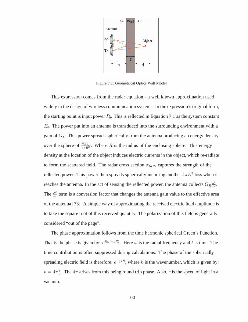
Figure 7.1: Geometrical Optics Wall Model

This expression comes from the radar equation - a well known approximation used

widely in the design of wireless communication systems. In the expression’s original form,

the starting point is input powerP0. This is reflected in Equation 7.1 as the system constant

E0. The power put into an antenna is transduced into the surrounding environment with a

gain ofGT . This power spreads spherically from the antenna producingan energy density

over the sphere ofP0GT

4πR2 . WhereR is the radius of the enclosing sphere. This energy

density at the location of the object induces electric currents in the object, which re-radiate

to form the scattered field. The radar cross sectionσRCS captures the strength of the

reflected power. This power then spreads spherically incurring another4πR2 loss when it

reaches the antenna. In the act of sensing the reflected power, the antenna collectsGRλ2

4π.

The λ2

4πterm is a conversion factor that changes the antenna gain value to the effective area

of the antenna [73]. A simple way of approximating the received electric field amplitude is

to take the square root of this received quantity. The polarization of this field is generally

considered “out of the page”.

The phase approximation follows from the time harmonic spherical Green’s Function.

That is the phase is given by:ej(ωt−kR) . Hereω is the radial frequency andt is time. The

time contribution is often suppressed during calculations. The phase of the spherically

spreading electric field is therefore:e−jkR, wherek is the wavenumber, which is given by:

k = 4π f

c. The4π arises from this being round trip phase. Also,c is the speed of light in a

vacuum.

100

Up to now only the standard radar equation has been introduced with a square root to

approximate electric field and a phase term that comes directly from the 3D time harmonic

Green’s Function. Now, the wall is introduced. To handle it,we assume that the incident

wave is a time harmonic plane wave. This means that the wall isconsidered to be an

infinite slab of homogenous material with a constant permittivity ǫ2 and thicknessτ .

Penetration of the electric field is governed by the Fresnel transmission coefficientsT12 and

T21. The electric field amplitude is attenuated inside the material by a frequency dependent

dampening factor:e−2ατ . And, finally, the phase term inside the wall is governed by

e−2jβτ .

This completes the pieces of the EGO model as described by Equation 7.1. Note that

T12 andT21 correspond to the transmission coefficient from free space into the material

and from the material into free space respectively. These coefficients are squared because

the wall is traverse twice in the round trip.

The model can be expanded to include the response of the wall.Equation 7.1 shows the

direct return from the front of the wall as implied by Figure 7.1. A more complete model

would include the return from the back of the wall and also multiple bounces between the

front and back.

E ′R(f, x) = E0

[(√

GT GR

(4πh2)2

(λ)2

4π

)

R12

]

e−j2kh (7.2)

This expression is derived using similar arguments to Equation 7.1. In this case the

Fresnel reflection coefficientR12 is used to capture the field reflected from the front of the

wall interface. The final observation made by the monostaticradar is the sum of the return

from the object and the return(s) from the wall.

101

Figure 7.2: Geometrical Optics Bistatic Model

Bistatic RADAR Model

The virtual transmitter concept places (virtually) an omnidirectional transmitter inside the

building being imaged. It does this by generating a buildingmodel composed of discrete

scattering elements. A numerical electromagnetic prediction of the fields produced by

the virtual transmitter is computed for locations outside the building. This field is used to

predict locations where the best measurement conditions exist from which to re-illuminate

the location of the transmitter.

To support this stage of the algorithm, an extended geometrical optics model for

forward scattering has been developed. This model is calledbistatic because the receiver

and the transmitter are not co-located. Figure 7.2 illustrates the concept.

ER(f, x) = E0

[(√

GT GRλ2

((4π)3R2sR

2t

σRCS

)

T12T21e−αχe−jβχ

]

e−jk(Rs+Rt−χ) (7.3)

The bistatic model is mathematically developed with similar arguments as the

monostatic model. Equation 7.3 is the result.

Here the parameterRs is the distance from the transmitter source to the scattering

object,Rt is the distance from the object to the receiver, and,χ is the straight line distance

of the path within the wall medium. In this bistatic version,the radar cross sectionσ is the

non-backscatter RCS. For simplicity, this parameter is considered constant regardless of

the illumination and observation directions. This does notin general have to be true. The

scattering objects could have directional qualities, which would be represented by an RCS

102

functionσ(θ, φ). Note that this expression no longer contains round trip distances.

The direct path from the transmitter to the receiver passes through the wall.

Equation 7.4 describes the link including the wall’s contribution. TheRr parameter is the

transmitter to receiver distance.

E ′R(f, x) = E0

(√

GT GRλ2

(4πRr)2

)

T ′12T

′21e

−αχ′

e−jβχ′

e−jk(Rr−χ′) (7.4)

The observed field measured by the receiver is the sum of Equation 7.3 and 7.4.

7.2 The Outer Wall Problem

Approximations and simulations are used in this work to gainphysical insight into the

spatial signatures produced by objects observed by surfacepenetrating radar. The radar

system is a receiver/transmitter pair that scans along the outside of a building. The returns

can be used to produce an image (slice) of the interior of the room.

The imaging approach used in this work is wavenumber migration. It was first

introduced in synthetic aperture radar imaging by [62]. Themethod was first developed

for seismology [63], [74]. The principal contribution of this paper is the application of this

approach to See-Through-The-Wall radar imaging.

The wavenumber migration algorithm works as follows. The 2Dcomplex spectrum

of the image is constructed by properly reformatting the plane waves received by the

radar system. The reformatting requires exact knowledge ofthe phase of the propagating

waves. When a wall of unknown thickness and permittivity is introduced, the algorithm

can no longer focus the image because the wall imposes an unknown delay on each plane

wave due to the decreased and unknown propagation speed within the wall. To properly

reformat the waves, the wavenumber migrator must know the bulk effect of these two

parameters (unknown permittivity and unknown thickness) and remove that phase delay

from the recorded data.

103

Adding to the complication of this problem is the fact that the reflection coefficients

of the wall are unknown. In this work we will assume that the radar return from the wall

is composed of a reflection from the front surface and a reflection from the back surface.

These two returns sum together to form a signal in noise with two unknown reflection

coefficients and one unknown phase. Due to the non-linear nature in which these three

parameters manifest themselves in the returned signal, some assumptions will have to be

made in order to estimate them. Two approaches can be considered.

The first approach assumes that the reflection from the wall surface has been removed

by some other means. This greatly simplifies the problem and allows for the back of the

wall reflection coefficient and the phase at all required frequencies to be removed using

a sine and cosine or dual phase technique. This approach is, therefore, a non-parametric

approach that estimates the phase at all frequencies. In practice, it may be a significant

technical challenge to eliminate the surface reflection contribution as required by this

method. Therefore, a second technique is proposed.

The second technique is a dual frequency approach. Here it isassumed that the

frequencies are close enough together so that the reflectioncoefficients of the wall

are nearly constant in frequency. The phase unknown is reduced to its fundamental

unknown part, which is the product of the wall thicknessτ and the square root of the wall

permittivity√

ǫ2. By relying on a cross-demodulated signal (that is a transmitted cosine

mixed with a sine on receive) the wall return is naturally rejected. Two separate soundings

are made at the two frequencies. After the cross-demodulation the reflection coefficient of

the back of the wall and the phase parameter are non-linearlycoupled within the signal.

A non-linear iterative maximum likelihood estimation approach is used to separate these

two parameters via the Newton-Raphson algorithm. When this algorithm converges, it

provides a parametric estimate of the thickness-permittivity-squareroot product. With this

estimated parameter, the phase delay for any frequency of interest can be predicted.

We adopt a physical optics model for electromagnetic wave propagation for a simple

104

Figure 7.3: Three Point Scatterer Simulations

environment consisting of three point scatterers placed behind the wall. These simulations

are used to show the result of correcting the imaging signalswith the estimated phase.

Images produced without phase correction are also providedto demonstrate the need for

correcting unknown phase distortion.

7.2.1 Point Target Simulations

The simulation consists of a stepped frequency radar generating frequencies from 500MHz

to 2.5GHz with equal steps, a homogeneous wall, and three point scatterers. Figure 7.3

shows the point scatterer arrangement. The radar is pointeddirectly at the wall. The

imaging algorithm operates on a measurement of radar backscatter at 256 frequencies

observed at 201 locations parallel to the wall. We define a local coordinate system (also

shown in Figure 7.3) at a specified center of the generated image.

We employ a physical optics model of radar wave propagation through the medium.

Specifically, the radar rf field is mathematically modeled asplane waves. The reflections

from the wall and back of the wall are governed by Fresnel Reflection Coefficients, which

are valid for time harmonic plane waves. For this work, refraction effects predicted by

Snell’s Law have been ignored for simplicity. Snell’s Law predicts that the waves will be

bent as they enter and leave the non-free space media In this paper we neglect this effect

and assume that the waves travel straight through the wall regardless of angle of incidence.

105

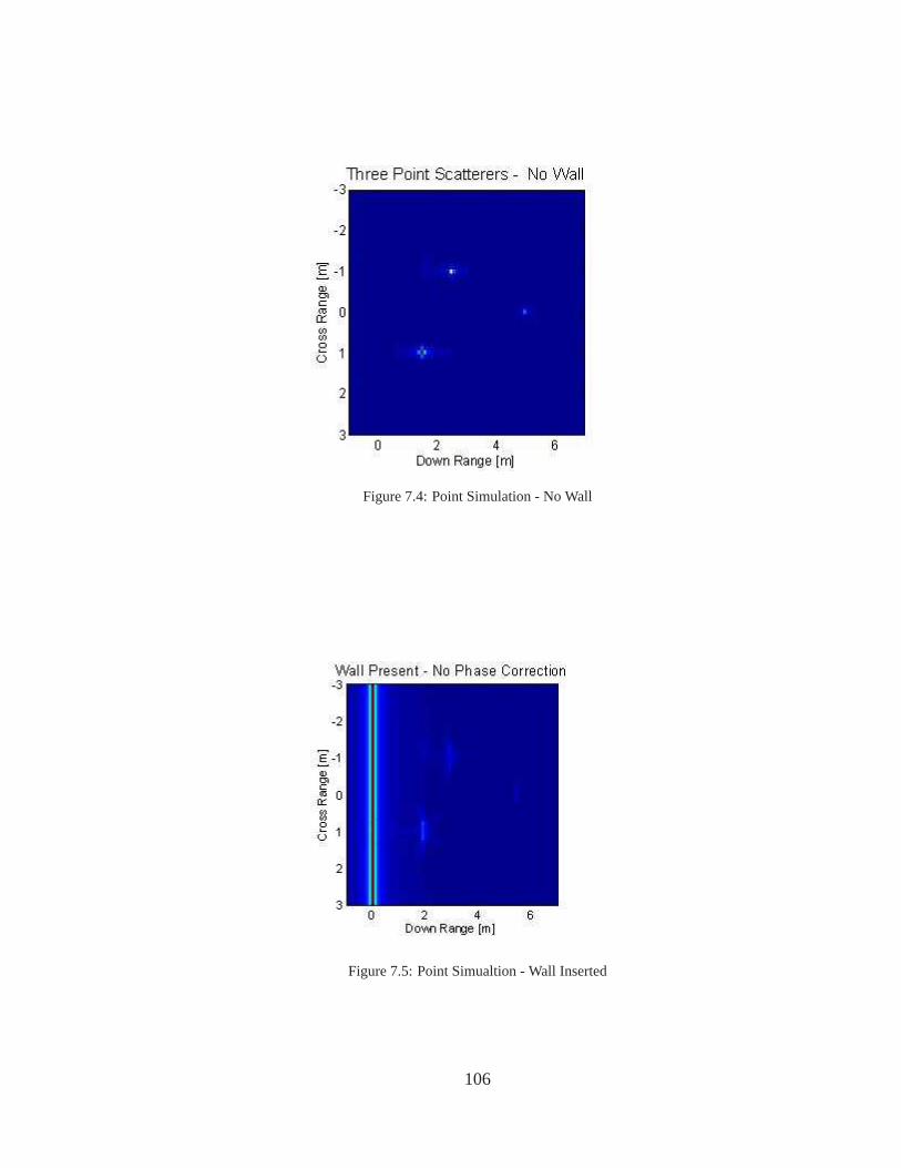
Figure 7.4: Point Simulation - No Wall

Figure 7.5: Point Simualtion - Wall Inserted

106

The imaging algorithm used to reconstruct the image of the three point scatterers is

wavenumber migration. This method transforms the receivedsignals into the 2D frequency

space and manipulates the phase of each wavenumber. Interpolations (i.e. resampling) is

also applied to format the data properly in preparation for a2D inverse FFT. With correct

interpolation and phasing, the energy of point scatterers become focused [63]. This can

be seen in the free space (no wall) simulation shown in Figures 7.4 & 7.5. The 3 point

scatterers are clearly well focused into point targets in this simulation. Their amplitudes

can be seen to fade for targets that are further away from the wall. This is due to the1r2

spherical spreading of the energy in the transmitted wave. In these simulations the radar

is just 6 meters from the farthest point scatterer. At these distances beam divergence loss

of the transmit energy can’t really be ignored. The point targets have the same radar cross

section (10dB).

Figure 7.5 shows the motivation of this work. When the wall is inserted between the

radar and the point scatterers, the imaging algorithm cannot focus the points. This is due

to an unknown phase factor that is now present in the data stream. A simplified model of

the observations is given by Equation 7.5.

y(f, x) = ap(f)e−jφp(f,x)aw(f)e−jφw(f,x)ρne−jφn (7.5)

The amplitude and phase labeledap andθp are due to the free space propagation

between the radar and thenth point scatterer. The complex reflectivity of the scatterer is

given in amplitude byρn andφn. The effect of the wall is to produce an attenuation and

phase (both of which are unknown) given byaw andφw.

Under this model the wall acts as a filter that attenuates someof the incident energy. If

this is a function of frequency, it would have to be estimated, if the goal is to reconstruct

the true reflectivity of all the pixels in the image. On the other hand, if the goal is to

reconstruct the location of the scatterers in the image, theamplitude attenuation can be

107

ignored [63]. Of course, in the presence of noise or interference the power transmitted

by the radar must be enough to provide a usable signal-to-noise ratio of the received

amplitudes. The effect of the phase w is to distort the reconstructed image. Hence

the phase must be estimated explicitly prior to image reconstruction Note that the wall

parameters are the same for all simulations in this work: relative permittivity of the wall is

10 and it is 0.2 m thick.

7.2.2 Wall Phase Determination and Correction

Two methods are proposed here for determining the phase caused by a wall of unknown

permittivity and unknown thickness. Both methods utilize a pulsed radar. The pulses

contain a cosine waveform with just 1 frequency that lasts 100 µsec. The return signal is

assumed to be a superposition of two cosine functions. The first is from the surface of the

wall and the second is from the back of the wall. Equations 7.6and 7.7 shows the expected

return.

r(t) = a0cos(ωt − φp) + a1cos(ωt − θ − φ) + n(t) (7.6)

θ =4πf

ch (7.7)

φ =4πf

cτ√

ǫ2 (7.8)

Theθ parameter is the expected phase delay due to the waveform propagating to the

wall surface and back to the radar. It is reasonable to expectthis value to be known. The

φ parameter, on the other hand, contains theτ√

ǫ value that is unknown. Theα0 andα1

values are related to the reflection coefficients of the frontand back wall surface. The

108

noisen(t) is an unknown, performance limiting factor.

Dual Phase Approach

The first approach demodulates the returned pulse with a cosine and a sine waveform. This

would be the same as transmitting a cosine and a sine signal and demodulating them both

with a cosine. The result is an in-phase and quadrature measurement.

R(ω) =1

N

N∑

i=1

r(ti)cos(ωti − θ)R(ω) =a0

2+

a1

2cos(φ) (7.9)

Q(ω) =1

N

N∑

i=1

r(ti)sin(ωti − θ)Q(ω) =a1

2sin(φ) (7.10)

Equations 7.9 & 7.10 show the processing steps and the final scalar values. It is

assumed that the sampling rate is sufficiently high to prevent aliasing. Note that all the

unknown parameters appear in these scalar measurements. A separate measurement must

be made at each frequency used in the imaging system.

A significant issue exists in the in-phase value. Thea0 term is the reflection coefficient

of the wall surface. This value must be determined prior to the application of this dual

phase method. This is the so-called ”layer peeling”. The wall surface must be determined,

then the inner wall structure, then the imaging of the area behind the wall. Here we focus

only on the solving of the middle problem - the inner wall structure. With the removal of

thea0 value, the in-phase measurement becomes what is shown in Equations 7.11

R(ω) − a0

2→ R(ω) =

a1

2cos(φ) (7.11)

Now the form of the in-phase and quadrature values can be divided to remove a1

(unknown). The result is a tangent of the unknown phase. By taking an arctangent, the

109

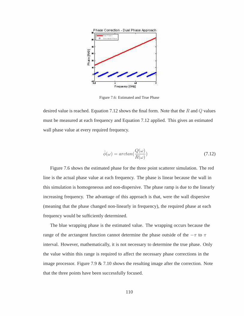
Figure 7.6: Estimated and True Phase

desired value is reached. Equation 7.12 shows the final form.Note that theR andQ values

must be measured at each frequency and Equation 7.12 applied. This gives an estimated

wall phase value at every required frequency.

φ(ω) = arctan(Q(ω)

R(ω)) (7.12)

Figure 7.6 shows the estimated phase for the three point scatterer simulation. The red

line is the actual phase value at each frequency. The phase islinear because the wall in

this simulation is homogeneous and non-dispersive. The phase ramp is due to the linearly

increasing frequency. The advantage of this approach is that, were the wall dispersive

(meaning that the phase changed non-linearly in frequency), the required phase at each

frequency would be sufficiently determined.

The blue wrapping phase is the estimated value. The wrappingoccurs because the

range of the arctangent function cannot determine the phaseoutside of the−π to π

interval. However, mathematically, it is not necessary to determine the true phase. Only

the value within this range is required to affect the necessary phase corrections in the

image processor. Figure 7.9 & 7.10 shows the resulting imageafter the correction. Note

that the three points have been successfully focused.

110

Figure 7.7: Image After Correction with Dual Phase Approach

Dual Frequency Approach

The dual phase approach makes an assumption that may not be practically achievable.

This is the assumption that the return from the front of the wall has been removed (i.e.

canceled). Because of this a second approach is introduced here. Some assumptions must

also be made for this method. Two frequencies will be used to generate a set of non-linear

equations that will be solved iteratively using a non-linear, successive approximation

method. The assumptions here are that the reflection coefficients remain constant for the

two frequencies. Since these values are slowly varying in frequency, this assumption is

very nearly true. As long as the frequencies do not get too farapart, this assumption will

hold.

Our starting point is with the quadrature measurementsR andQ at two frequencies

f1 andf2. The reason for using quadrature is that thea0 unknown is naturally removed

during the demodulation process. If we also consider the in-phase measurements, we have

to solve for the addeda0 unknown. Sincea0 anda1 are nuisance parameters, we utilize

only q1 andq2. The expressions for these measurements are given by Equations 7.13-7.16.

These are rewritten in the form of functionsF1, F2 for use in the Jacobian matrix described

next.

111

q1 =a1

2sin(φ1) (7.13)

q2 =a1

2sin(φ2) (7.14)

F1(x¯) =

x1

2sin(

4πf1

cx2) (7.15)

F2(x¯) =

x1

2sin(

4πf2

cx2) (7.16)

J =

δF1(x)δx1

δF1(x)δx2

δF2(x)δx1

δF2(x)δx2

=

12sin(4πf1

cx2)

x1

2sin(4πf1

cx2)

4pif1

c

12sin(4πf2

cx2)

x1

2sin(4πf1

cx2)

4πf2

c

(7.17)

The parameterx1 is the reflection coefficient from the back of the wall. The parameter

x2 is the thickness-permittivity-squareroot product. Thex2 parameter is of primary

interest. Knowledge of this value allows for the phase distortion to be corrected.

Define the two element vectorsq andF by contacting the two respective terms

in Equations 7.13-7.16. The problem of estimating the parametersx1 andx2 can be

formulated as a non-linear least squares problem,minx(|q − F (x)|2), equivalent to

maximum likelihood under an additive Gaussian noise modelq = F (x) + noise. Starting

with an initial value ofx1,x2, we can find the least squares solution using the iterative

Newton-Raphson approach. This algorithm uses successive approximations to iterate to a

solution. The Jacobian matrix shown in Equation 7.17 is determined using the non-linear

equationsF1,F2.

The Jacobian matrix defines a hyper-plane that is tangent to the manifold of theF1,F2

112

functions at the point of the current estimates ofx1,x2. A solution to the equations is

found within this plane and this solution will be closer to the true answer than the previous

estimates. The same is true for the next solution until the estimates no longer change.

This is the successive approximation strategy. Mathematically, this can be written as in

Equations 7.18 - 7.21.

x¯k = xk−1 + (JT

k−1Jk−1)−1JT

k−1(q¯− F

¯(x¯k−1)) (7.18)

q¯

=

q1

q2

(7.19)

x¯

=

x1

x2

(7.20)

F¯(x¯) =

F1(x¯)

F2(x¯)

(7.21)

A logical starting point is to choose the initial values ofx1,x2 to determined by the

values we expect (i.e., the mean values) for the wall being interrogated. This incorporates

the a priori information we have about the wall. For this simulation only a few iterations

are required for the estimates to converge. Figure 7.8 showsthe convergence in thex1

parameter while Figure 7.9 shows the same forx2. The starting values were 0.8 forx1

and 0.6 forx2. The actual values were 1.0 and 0.6325 respectively. The estimated values

reached by the algorithm were 1.3 and 0.6270.

Thex2 parameter corresponds to the product, which is the key element in the unknown

phase experienced by the waves traveling through the wall. Once this parameter is

113

Figure 7.8: Convergence of Parameterx1

Figure 7.9: Convergence of Parameterx2

114

Figure 7.10: Image After Correction with the Dual FrequencyApproach

estimated, the image can be phase corrected at any frequency. So, provided that the

wall structure does not change, only one sounding has to be made in the dual frequency

approach. The resulting image is shown in Figure 7.10.

Note that the three point scatterers are well focused in Figure 7.10. The dual frequency

method shows much promise. Unfortunately, it does have challenges to be addressed in

future work, namely local minima of the objective function‖q − F (x)‖2 [75].

7.2.3 Outer Wall Conclusion

Two approaches have been proposed for determining the unknown phase produced by

plane waves propagating through a wall. It has been shown that this unknown phase

prevents proper imaging of the scene behind the wall using a See-Through-The-Wall radar.

Both approaches were effective in determining and removing the unknown phase when

their underlying assumptions were satisfied.

The two approaches were also quite robust when contaminatedwith noise. Both

functioned well at a signal-to-noise (SNR) of -10dB. (SNR hereis defined as the mean

squared amplitude of transmitted sinusoid to the variance of the noise.) This robustness is

due to the correlating of the return signal with the transmitsignal. Each pulse was sampled

115

in such a way that 1000 points were collected. When all these samples are correlated with

the signal and averaged together, a reduction in noise variance of a 1000 is affected.

7.3 The Inner Wall Problem

One of the goals of STW radar is to generate a layout map of the interior of buildings.

When the radar frequency is sufficiently high methods like Method of Moments and

Finite Element become intractable. Here we propose the use of scattering center models

of objects like dihedrals, tophats, cylinders, and spheresas an approximate method for

simulating radar response. These scattering primitives can be associated with the objects in

the scene. By identifying the primitives, a layout of the building interior can be generated.

The contribution of this section is in the area of inner wall mapping. Others have

looked at the problem of determining the characteristics ofthe outer wall [76] [77] . A

great body of research exists on the identification of objects found in synthetic aperture

radar imagery [78] [79] [80] . The issue of dealing with and mapping inner walls is a

problem unique to STW radar imaging. The approach taken hereis to look at the inner

walls as dihedral scattering primitives. Dihedrals have a ”two bounce” characteristic that

can be identified using polarimetric radar. This approach has been explored in the area of

Foliage Penetrating Radar [3] [81] [2] for discriminating trucks from trees.

7.3.1 Inner Wall Simulation

Simulations of radar imagery are employed throughout this study. A building scene

contains several basic components: 1) an outer wall, 2) a setof inner walls, and 3) a

collection of objects. Of particular interest is the existence of any weapons stored inside

inner rooms.

Note that the scene of Figure 7.16 is sparse. This means thereis a lot of empty space.

A Method of Moments (MoM) approach to modeling this scene might appear to be a good

starting point. The MoM approach only deals with the scattering objects within the scene.

116

Other approaches like Finite Difference Time Domain (FDTD)and Finite Element Method

(FEM) will ”grid up” all pixels including the empty space. The rule of thumb in all E&M

modeling applications is for the discretization to have tensamples across the shortest

wavelength. The building here is 10m x 10m in dimension. At 5GHz this translates to

1.3 million elements in the outer wall (considering only theintegrals over the surfaces)

and 300 thousand elements in the inner walls, which are 3m long. Inverting a matrix of

this size to solve for surface currents would require powerful computing. As an alternative

to large numerical simulations, we make several simplifying assumptions. The primary

assumption is that a enhanced geometrical optics approach is sufficient.

EGO is discussed in Section VII. It assumes that propagatingwaves can be modeled as

plane waves. In this STTW application the outer walls are modeled using Fresnel reflection

and transmission coefficients. This implies that the wall islarge and homogenous. The

physics of the corners are not truly captured. For cases where the corners are not within

the footprint of the antenna beam, this assumption should beadequate. In addition, the

walls are considered to have no windows, doors, or other openings. The outer walls are

assumed to be reasonably thick - on the order of 0.2m.

The inner walls are simulated using the scattering center approach. A dihedral is

formed by the connection between the wall and the floor. The primary goal of this work

is to determine the inner structure of the building. This means identifying inner walls and

separating them from other objects to form abuilding model from the gathered data.

Modeling the inner walls as dihedral scattering objects will not provide a high fidelity

prediction of scattered fields. It will, however, capture the polarimetric characteristic of the

wall’s response. This will allow for testing of polarimetrybased algorithms for identifying

the inner walls. The assumption that the inner walls can be modeled as dihedral scattering

centers should be adequate for thin inner walls. This means that the radar wave passing

through the wall will experience little phase delay and little attenuation due to the inner

wall.

117

Figure 7.11: Dihedral Scattering Center

Objects within the scene are considered to be point scatterers with varying scattering

cross sections. For simplicity, the objects are simulated as constellations of points. All

objects within the scene represent potential objects of interest. The goal here is to classify

the outer walls, inner walls, and scene objects. In future work the scene objects can be

further processed to identify the object class.

Using the scattering center approach, Figures 7.12 and 7.13were generated. These

are produced by illuminating the scene of Figure 7.16 from the bottom (Figure 7.12)

and from the left (Figure 7.13). The simulated radar has a bandwidth of 1GHz about a

center frequency of 4.5GHz. This frequency is relatively high compared to most existing

surface penetrating radar systems. The frequency range waschosen to lend validity to the

EGO assumptions underlying these simulations. The beamwidth of the antenna is90o in

both cross range directions, this beamwidth is intended to match a man portable (hand

held) antenna. Likewise, the stand-off distance is 10m corresponding to a system taking

measurements from a nearby road.

Several noteworthy items can be seen in these simulations. First of all, the inner

walls parallel to the radar line-of-sight tend to vanish. This occurs in spite of the large

beamwidth of the antenna. At the wavelengths used in these simulations, there is not much

direct backscatter from the inner walls when they are not perpendicular to the radar’s

line-of-sight. The perpendicular walls do have a small response. These are the edge

118

Figure 7.12: Inner Wall Simulation - Bottom Illumination

Figure 7.13: Inner Wall Simulation - Left Illumination

119

diffraction effects (slightly visible) at the edges of the dihedral. Looking at the simulated

sink, the reflectance of objects appears to change between the two images. This is due to

the spherical spreading of the power emitted by the radar. InFigure 7.12, the illumination

is from the bottom. In Figure 7.13, it is from the left. The radar is physically closer to the

sink in the bottom illumination. Since the imaging algorithm does not attempt to correct

for spherical spreading, the reflectance appears to become weaker in the left illuminated

scene.

7.3.2 Layout Mapping

The goal of this work is to determine aBuilding Model from observed imagery. This

is similar to a Computer Aided Design (CAD) drawing of the building. This drawing

captures the internal layout. To create this product, it is necessary to identify the outer

walls, inner walls, and scene objects. These are then storedto theBuilding Model file

as objects. To ensure that all inner walls are captured, it isnecessary to scan the building

from two directions - bottom and left. This insures that all inner walls will be illuminated

by the radar beam.

A simple approach to detecting inner walls is to take advantage of the dihedral-like

response that is formed by the intersection of the walls withthe ground. Polarimetrically,

we expect the phase angle of the VV to HH ratio to be 180 for dihedrals. This occurs

because the VV polarized wave sees a 180 phase shift while theHH polarization does not

have a corresponding phase shift. This fact can be exploitedto help map the inner walls of

the structure.

Figures 7.14 and 7.15 show the result of applying a simple dihedral scattering center

detector. This detector takes a ratio of the VV and HH compleximages and finds the pixels

with a phase close to 180. The resulting pixel maps correspond to the inner walls. These

regions can then be modeled as inner walls in theBuilding Model.

120

Figure 7.14: Detected Inner Walls - Bottom Illumination

Figure 7.15: Detected Inner Walls - Left Illumination

121

7.3.3 Inner Wall Conclusion

This section explored the issue of simulating building penetrating radar with a focus on

inner wall detection. The simulations were conducted in a frequency range where EGO

was expected to dominate. The resulting simulated images were used to propose an inner

wall detection and mapping algorithm. The algorithm utilizes polarimetric scattering

characteristics to classify pixels as part of the inner walls. Encouraging preliminary results

are presented.

7.4 I.R.I.S. Adaptive Imaging

See-through-the-Wall Radar Imaging is an emerging technology useful to both Homeland

Security and Law Enforcement. The goal is to provide an imaging tool that gives

authorities information. The nature of this information includes the internal layout of

a building (location of doors, obstructions, or inner rooms), the existence and location

of objects of interest(weapons, methamphetamine labs), and the tracking of suspicious

individuals inside. This application is challenging because it requires the processing

and interpretation of electromagnetic waves in an inhomogenous media with unknown

material parameters and structures. To provide the optimalmeasurement, it is desired

to adapt the observations to a location and/or frequency range that will provide the most

powerful information. The proposed approach makes use of a ”virtual transmitter”. The

fields observable from the virtual transmitter are predicted from a ”building model” that is

determined from previous observations. By reciprocity, thefields observed on the outside

of the building reflect the fields that can penetrate the building from that outside location to

illuminate the location of interest. Because the building model must be built up (learned)

over the course of several measurements, the algorithm is iterative. An interesting location

within the building is determined after the first measurement. An initial building model is

produced form this observation, the virtual transmitter isplaced, and the fields outside the

building are predicted using numerical electromagnetic models. After each observation,

122

Figure 7.16: 2D scenario used to illustrate the IRIS approach. Room is10 × 10 meters and a SAR sensorwith 1 meter baseline can be placed at any position parallel to top or bottom walls at exterior of building.

more information is obtained about the building and the building model is updated. This

may lead to a new placement of the sensor for the next observation. It may also lead to

new locations of interest that should be interrogated by theimaging sensor.

Assume an initial sensor/illuminator configuration has been deployed and that an

image has been reconstructed along with its confidence map using the iterative Bayesian

algorithm described in Sec. II. The objective of IRIS is to finda new sensor configuration

that will allow us to improve upon the initial reconstructedimage. For concreteness,

we focus on imaging the interior of a building and assume thatthe space of possible

configurations are locations where the baseline of a small SAR sensor could be placed at

the building exterior (see Fig. 7.16). The proposed IRIS approach uses the confidence

map to identify regions of the image that were poorly resolved, i.e., pixels that have

poor confidence values (P (xi = 0|Y ) near 0.5). It then simulates the RF field at the

building exterior that would be created by placing a (virtual) transmitter in one of the poor

confidence regions of interest. From this simulated field we can extract information about

the best location to redeploy the illumination/sensing platform.

For this purpose we define the predicted information gain as ameasure of how much

a given sensor position might enhance the ability to detect the presence or absence of a

scatterer in the vicinity of the virtual transmitter. The value of redeploying the sensor

123

Figure 7.17: Iterative reconstruction of building interior illustrated in Fig. 7.16 after 10 iterations and a full10 meter baseline (left) and 1 meter baseline (right) monostatic SAR illuminator/sensor.

at a particular location can be measured by the variation of the RF field at that location

produced by perturbing the location of the virtual transmitter. Define the energy frequency

spectrumEx,y(ω) of the RF field measured at locationy due to an omnidirectional

transmitter placed at locationx, and for a locationxk defineEk = Exk,y. The spectral

variation produced by perturbing the locationx from a reference locationx1 to a new

locationx2 can be measured by the Kullback-Liebler (KL) divergence

D(E1‖E2) =

∫

E1(ω) log

(

E1(ω)

E2(ω)

)

dω.

The KL divergence and its generalizations have been used by many authors in sensor

management problems and are often referred to as the information gain [43] [82] [83]. We

define the information gain at sensor positiony as the sum of the KL divergences of the

RF fields produced by cross-range perturbationx1 → x2 and range perturbationx1 → x3

of the virtual transmitter location:

IG(x, y) = D(E1‖E2) + D(E1‖E3). (7.22)

When viewed as a function ofy this quantity sweeps out the information gain field.

124

7.4.1 Numerical Simulation

We consider a scenario illustrated in Fig. 7.16. A weapons cache is hidden in a room

surrounded by four exterior walls and obscured by other interior walls and objects in the

room. A mono-static radar can be placed anywhere above the top wall or below the bottom

wall. The room is enclosed by a10× 10 meter wall that is 1/3 meter thick. We evaluate the

performance of a short baseline (1 meter) SAR sensor that canbe placed at any position

along the 10 meters of the top or bottom wall at 1 meter standoff distance. The operating

frequency of the simulated radar was 4.0GHz to 5.0GHz and theSAR radar baseline was

sampled at 10 points (every 10cm) along its 1 meter extent. The simulator modeled each

object on the room with a simple superposition of scatterersusing physical optics. We

assume that the external wall attenuation and phase parameters are accurately estimated,

e.g using the method of [76].

For an initial sensor position centered at the middle of the lower wall the two panels of

Fig. 7.17 show the results of applying ten iterations of the Bayesian iterative reconstruction

algorithm (6.30) with sparseness prior (6.29). The values of a, w andσ were fixed during

the entire experiment. The right panel of the figure is significantly lower resolution

than the left panel due to its relatively smaller baseline of1 meter. The left panel is the

reconstruction obtained after the first iteration of the IRISprocedure.

The probability mapP (xi = 0|Y ) and the associated entropy map− log P (xi =

0)− log P (xi = 1) are shown in Fig. 7.18. The entropy map is maximum for reconstructed

pixels whosea posterioriprobability of being empty space is close to 1/2. The entropy

map therefore measures thea posteriori(lack of) confidence in the value of that pixel and

is called the “confidence map” of the image. From the confidence map a region of low

confidence is identified, e.g., the region near the top of the image, and a virtual emitter

is simulated in this region to generate an information gain field for determining the best

redeployment configuration for the next iteration of IRIS.

The construction of the information gain field is illustrated in Fig. 7.19 for the scenario

125

Figure 7.18: Confidence Map (left) and Entropy Map (right) associated with the 1 meter baseline imagereconstruction shown in Fig. 7.17.

illustrated in Fig. 7.16 and a low confidence region region identified from Fig. 7.18. On

the right of the figure is the frequency spectrum of the induced RF field at a candidate

redeployment position at the exterior of the building for the three sensor positions

illustrated in the left panel of the figure. The difference between the reference spectrum

and the horizontally (cross-range) and vertically (range)perturbed spectra is measured via

the information gain formula (7.22). On the left of Fig. 7.19at the exterior of the building

is the color coded field corresponding to the information gain. The distances of the range

and cross-range perturbations of the virtual transmitter have been exaggerated for clarity

of presentation; actual perturbations would produce less obvious visual differences in the

RF spectra.

In Fig. 7.20 the virtual transmitter positions and induced information gain fields

are illustrated for iteration 2 and 3 of the IRIS algorithm. Optimal information gain

maximizing SAR positions are indicated by the 1 meter baseline white arrows at exterior

of the building. After the third iteration of IRIS 4 differentsensor positions will have been

deployed (including the initial deployment).

On the right panel of Fig. 7.21 a composite of the four reconstructed images (including

the final image) obtained from the three iterations of the adaptive IRIS algorithm described

above. The recovered resolution using IRIS’s total baselineof 4 meters is comparable to

126

Figure 7.19: The information gain field is computed by simulating the variability of the RF spectrum that avirtual transmitter in the vicinity of a pixel of interest (circle 1 in left panel) would generate at differentlocations at the exterior of the building. At right are the induced RF fields generated by a virtual transmitterat the reference position (circle 1), cross-range (circle 2), and range (circle 3) perturbations.

Figure 7.20: Virtual transmitter locations and the inducedinformation gain fields for iteration 2 and 3 ofIRIS for the scenario illustrated in Fig. 7.16.

127

Figure 7.21: Comparison between final IRIS reconstruction after 4 iterations with 1 meter baseline SARdeployments (shown by black arrows) versus one shot IRIS reconstruction using 10 meter baseline. In bothcases the reverse wavenumber migration model with EM implementation of MAP algorithm has been used.

the resolution of the non-adaptive one-shot 10 meter baseline shown on the left panel of

the figure.

7.4.2 Convergence

The nature of STW radar reveals that objects within the scenehave directional

characteristics. While many objects are omni-directional,the scattering objects that

compose the layout (that is the walls) are directional. Inner walls have narrow beam

scattering patterns. This means that a radar must be nearly perpendicular to the wall to

illuminate it. The illumination could come from either the “front” or the “back” side.

Corners have a wider beam. In contrast to inner walls, however, they will only backscatter

in one direction. Therefore, the radar must illuminate a corner from the proper side.

To insure complete detection of all scattering objects in a STW scene, a radar would

need to illuminate the entire360o aperture. Figure 7.22 shows the simulated test scene

imaged from full10m apertures on all four sides. The IRIS algorithm seeks to detect all

objects in the scene, while observing (much) less than the total 360o.

Convergence in the context of the IRIS algorithm is the notion that the image being

built adaptively will converge to the correct image. Since the algorithm is building the

larger scene from observations of small regions of the scene, it can be argued that the final

product will never truely to exactly the same as that observed by a larger aperture array.

128

Figure 7.22: Image from360o Aperture

However, the fundamental information contained in the image can be the same. For this

reason the quantity of interest in convergence is the “probability of detection” of the scene

objects.

Figure 7.23 shows the image and the apertures used in the finalversion of the IRIS

algorithm. All objects in the scene have been detected. Notethat the inner walls are tricky.

They have been detected by the1m aperture deployments, but are only partially revealed.

A way to overcome this is to use some other method to determinethe wall layout. This

could be through the deployment of an airborne asset that would collect the total3600 (or

40m) aperture or by making use of floor plans (if available).

For a useful concept of operation, the IRIS process must come to a final product with

less expense of resources (i.e. deployments, time, aperture used) than the full image.

Figure 7.24 shows the convergence process. To compare apples to apples the probability

of detection is plotted versustotalaperture used. Here we use meters because Figure 7.22

129

Figure 7.23: Image from IRIS

was produced from40m of total synthetic aperture by observing the10m per side scene

from all four directions.

Notice that two stall points are observed at3m and8m. These stalls are overcome

by an approach inspired by Yuan & Lin [84]. The alogorithm senses that it has reached

a stall and takes action to widen its search within the space of the scene. All objects are

detected after ten deployments. Necessary confidence in thescene is satisfied after twelve

deployments. Thus the IRIS converged in detection probability in 12m to produce Figure

7.23 rather than requiring the total40m used in Figure 7.22.

130

Figure 7.24: Convergence of Imaged Scene

131

CHAPTER VIII

CONCLUSION

8.1 Discussion of Results

This dissertation has addressed the problem of surface penetration with the goal of

detecting objects of interest. The general problem is one offorming an image with an

appropriate sensor, detecting points of interest within the image, and reporting objects of

intetest while rejecting clutter objects. The two main applications explored in this work

are landmine detection and surface penetrating radar imaging.

The first contribution chapter looks at non-statistical approaches to image under-

standing, signal-to-noise ratio enhancement, and object classification. First, computer

vision techniques are used to segment a ground penetrating radar image into target and

background regions. A bounding box around the signature is used to determine the object

depth and size. Next, a novel approach to signal-to-noise ratio is introduced called the

hyperbola flattening transform. This transform applies to ground penetrating radar

signals, which have a hyperbolic point spread function. Thetransform helps to increase

the depth of penetration of the landmine by collapsing all the energy in the signature into

a point. The third approach applies basis projection operations to determine object depth

and size using electromagnetic induction (EMI) metal detectors. By identifying bases

derived from a magnetic dipole model of the scattered fields,a unique projection matrix is

formed for objects of varying depths and three canonical shapes.

The second contribution looks at statistical approaches. Because of a strong correlation

132

between object depth, type, and sensor response, pixel classification can be performed. By

modeling the response of two sensors (EMI and GPR) as a jointlydistributed Gaussian

mixture, the object type and depth can be determined by associating the pixel with a

specific Gaussian component. Using a Bayesian Network to facilitate training of the joint

probability density function is proposed and discussed. Statistical approaches are also

used in sensor scheduling. An approach calledActive Sensing is used to determine the

best single sensor to deploy from a set of six hypothesized sensors. It is shown by way

of a confusion matrix that the deployment of a single confirmation sensor can increase

the probability of correct classification of subsurface objects after detection of the objects

using the Gaussian mixture approach. Last in this contribution area a reinforcement

learning approach is explored for learning a policy that applies more than one sensor when

needed to produce the highest probability of correct classification with the least number of

sensor dwells.

The third contribution turns to imaging techniques. First,wavenumber migration is

explored for its ability to produce 2D and 3D imaging at an accelerated rate compared

to backpropagation techniques. The concept of image sparsity is introduced as a way

of reducing image artifacts. The key to implementing sparsity is the ability to perform

wavenumber migrationin reverse. With this technique, introduced in this dissertation,

Landweber iterations can quickly and efficiently transformdata between observation

and image domain. The final innovation of this work is appliedto See-Through- Wall

radar imaging. It is called the Iterative Redeployment of Illumination and Sensing (IRIS)

algorithm. This technique is a novel way of approximating a large synthetic aperture radar

system with multiple deployments of a much smaller array. The algorithm utilizes the

scene itself to determine the best locations to acquire further observations for the given

scene. E&M simulation tools dubbedvirtual transmitters are used to predict fields

outside the scene of interest. The tools are limited to Geometrical Optics, but use an

enchancement that corrects for phase distortions caused bythe outer wall. An information

133

gain metric is computed on the predicted external fields to direct sensor placement.

8.2 Suggestions for Further Research

Two decades of surface penetrating technology have been applied to the problem of

landmine detection and classification. Robotic arms are currently being implemented

on tactical vehicles to assist in the probing of suspicious locations. An arm that could

select a sensor of choice as directed by a sensor scheduling algorithm could result in high

rewards of accelerated performance. Such a device could especially reduce the impact of

interrogating non-threatening (false-alarm) objects.

The IRIS algorithm is composed of multiple subcomponents: 1)uncertainty map, 2)

sensor information map, 3) virtual transmitter, 4) sensor observations, and 5) imaging.

Each of these subcomponents is a potential field of research.For example, the imaging

approach used in this work drew upon the principle of image sparsity to control Landweber

iterations. Other mechanisms may exist that optimize various other prior information.

Also, the virtual transmitter here used compact models (Enhanced Geometrical Optics)

to simulate electromagnetic propagation through walls. A more accurate (and more

time/memory consuming) approach would be to use advanced numerical simulations

(MoM, FEM, FDTD) to give a high fidelity prediction to the external electric fields.

The utlimate goal in STW imaging is to create 3D volumetric images of entire

buildings. To accomplish this, high performance parallel computing will be required.

Parallel programming in conjunction with the fast and efficient imaging techniques used

in wavenumber migration could achieve a 3D result in a reasonable amount of time. These

techniques could also be utilized in 3D imaging of landmines. To date the Landweber

iterations using wavenumber migration approximations have been applied in “2.5”D. That

is, the algorithms have been implemented in 2D and applied to3D data in slices. A full

3D implementation of the algorithm is easily generalized and an excellent goal for future

research.

134

APPENDICES

135

APPENDIX A

ELECTROMAGNETIC INDUCTION (EMI) SENSORS

Metal detectors remain a useful tool for detecting buried metal objects. Fundamentally

they consist of a coil of wire that is driven by electric current. This current forms a

magnetic field that couples to the buried object. In responsethe object creates a secondary

magnetic field that can be sensed at the surface. This processgives this family of sensors

the name Electromagnetic Induction (EMI) sensors.

The primary challenge of these systems is separating the field they generate - called

the primary field - from the object’s response - called the secondary field. In this section

we study a typical EMI sensor called the EM61. This sensor operates in the time domain.

It generates pulses to create the primary field and measures the secondary field while the

primary field is off. Section A.1 describes the time responseof the system. It shows how

the time decaying signal can be used to identify the object’smetal content. Section A.5

describes the expected spatial signal formed by scanning over the object. Section 3.3.1

describes how to extract shape information from the spatialsignal.

A.1 EMI System Overview

The EM61 is the property of Geonics LTD of Toronto, Ontario. It is a man portable metal

detector capable of measuring mV changes in sensor response, and is shown in Figure A.1.

The device consists of a wire loop transmitter and two receiver coils mounted on wheels

to form a rolling platform. The main receiver is co-located with the transmitter while the

secondary receiver is 40 cm above it.

136

Figure A.1: The EM61 Metal Detector

The transmitter is continuously pulsed with current, whichcauses a primary magnetic

field to be emitted. This field induces swirling currents (called eddy currents) in the ground

below the device. If a target is present, the eddy currents inthe metal will continue to flow

for a short time after the primary field pulse is shut off. Thisforms a secondary magnetic

field that can be detected at the surface. The receivers sample and store the secondary field

during a small time window in between transmitter pulses. This insures that the secondary

field is not drowned out by the primary.

To operate the device over a survey area, the operator manually ”raster scans” the area.

That is the device is pulled back and forth across the area until it has been completely

covered. Samples are taken after each pulse of the transmitter. However, a counter on one

of the wheels triggers the receivers’ control electronics to average all samples received

since the last count. This is done to reduce noise. Thus, the slower an area is scanned, the

more samples over a single position will be averaged. Post test software maps the samples

into an image by utilizing along track positions recorded from the wheel counter and from

operator knowledge of the separation between scan lines.

A.2 Transmitter Waveform

One of the complications of designing an active metal detector is that the primary field

tends to overwhelm the secondary field produced by the target. This is due to the receivers

137

Figure A.2: Transmitter Current Waveform

being closer to the transmitter than they are to the target, as well as, the high power

necessary to produce a desired penetration depth. To prevent the primary field from

overwhelming the secondary field, the transmitter current is forced to zero as quickly as

possible on the trailing edge of the pulse and a sample of the secondary field is taken

at a time when the primary field has vanished. This technique is called time domain

electromagnetics (TDEM). (It is also referred to as eddy current analysis [85] in the

field of nondestructive evaluation.) Figure A.2 is a diagramof one period of the current

waveform that excites the transmitter. It is referred to as a”bipolar square wave with 50%

duty cycle”.

For the purpose of modeling the system’s operation, it is assumed that the transmitter

can be modeled as a vertical magnetic dipole. This is somewhat of a loose assumption

since the transmitter is a 1m x 1m square coil. However, investigation of experimental data

shows that this assumption is reasonable. Also, the ramp times are considered negligible.

What is important is the frequency at which the waveform in Figure A.2 operates and the

transmitter’s magnetic moment. Most models of the EM61 operate at a frequency of 75.0

Hz (period:T = 13.3ms). The magnetic moment,m0z, is given bym0z = NIA, whereN

is the number of turns in the coil,I is the magnitude of the current pulse, andA is the area

of the transmitter coil. The value of the magnetic moment forthis instrument is190Am2.

The transmitter waveform can be expanded in a fourier seriesthat is composed of a

component at75Hz and its odd harmonics (i.e.225, 375, 525Hz, etc.) [86]. In Section

A.4 it will be shown that the receiver filters out all frequencies but the75Hz fundamental.

So for the purpose of modeling, the transmitter is assumed tobe a vertical magnetic dipole

138

at75Hz with a dipole strength of190Am2.

A.3 Response of a Spherical Target

Many simplifying assumptions are used to approximate the response of a buried target

to the primary magnetic field. The approach outlined here is asummary of the research

conducted by Y.Guo, which is documented in a Johns Hopkins University/Applied Physics

Laboratory technical note [87].

It has already been assumed that the transmitter is a magnetic dipole. Another

assumption is that the target is a solid, metallic sphere buried in a conducting half

space with a homogeneous conductivity. The problem of quantitatively determining the

secondary field produced by the sphere is found in an article by Hill and Wait [88]. Their

approach is to determine the magnetic field at the center of the spherical target with the

target removed. This is called the unperturbed field. This field is decomposed into vertical

and radial components that induce magnetic dipoles in the sphere. The expressions relating

the unperturbed magnetic field to the vertical and radial induced dipoles are:

mz = −2πa3P (ω, µs, σs, a)H0z(xs, ys, zs) (A.1)

mr = −2πa3P (ω, µs, σs, a)H0r(xs, ys, zs) (A.2)

P (ω, µs, σs, a) = −2µs (sinh α − α cosh α) + µ0 (sinh α − α cosh α + α2 sinh α)

µs (sinh α − α cosh α) − µ0 (sinh α − α cosh α + α2 sinh α)(A.3)

α = (iωµsσs)12 a (A.4)

139

Figure A.3: Phenomenology of Induced Dipole Sources

The target parameters are:a the radius,µs andσs the magnetic permeability and

electric conductivity,(xs, ys, zs) the target’s center of mass position with respect to the

transmitter.ω is the transmitter frequency andµ0 is the permeability of free space. The

functionP is called the polarizability. Note that this factor is the same for both the vertical

and radial induced dipoles. This is because the target is a sphere (i.e. all directions are

equally polarizable). Figure A.3 illustrates the induction of horizontal and radial dipoles

by a vertical magnetic dipole transmitter.

Once the response dipoles have been induced, the secondary fields at the surface are

determined by the standard equations for the magnetic field due to a magnetic dipole

buried in an infinite conducting half-space. These expressions and the expression for the

unperturbed field can be found in [33]. Qualitatively, the fields of the induced dipoles are

shown in A.3.

The magnetic field measured at the surface will be a superposition of the fields of

the horizontal and vertical induced dipoles. Along with thethree major assumptions

already pointed out, the expressions in Equations A.1 through A.4 carry with them several

additional assumptions. For the sake of clarity, all assumptions concerning this simplified

target response model are now listed.

(1) The transmitter is a point magnetic dipole.

140

(2) The target is a solid, metallic sphere.

(3) The target is buried in an infinite conducting half-spacewith homogeneous

conductivity.

(4) The sphere must be electrically small. This means that the radius of the sphere

must be small compared to the wavelength of the transmitted pulses. This is always true

for the EM61 case since a transmitter at75.0Hz has a wavelength of4000km.

(5) The sphere must be located a sufficient distance from the source/observer. This

insures that higher order multipoles can be ignored.

(6) The sphere must be buried a sufficient distance from the interface. This insures that

the interaction between the induced dipoles and the interface are unimportant. It has been

shown that the sphere-interface separation should be at least two sphere radii [88].

(7) The induced electric dipole moment is negligible. In addition to the vertical and

radial magnetic fields, a vertical dipole on the surface alsocreates an electric field in

the azimuthal direction, which circles the vertical axis. This electric field will induce an

electric dipole moment in the target that will contribute tothe vertical magnetic field on

the surface. The electric dipole contribution is negligible for low frequencies (i.e. under

10 kHz), which is always valid for the EM61.

A.4 Receiver Characteristics

This section discusses how the secondary magnetic field is converted into a voltage at

the output of the receivers. There are two approaches that could be taken. The first is to

consider the primary magnetic field as being excited by a change in the DC level of the

transmitter current. After the primary field has been zeroed, the secondary field decays

exponentially with the following form [89]:

Hs(t) = Ae−tτ (A.5)

141

τ =

√

σsµsa2

π(A.6)

HereA is the strength of the magnetic field at the instant before thetransmitter current

is brought to zero.τ is the time constant of the secondary field decay witha, σs, and

µs corresponding to the radius, conductivity, and magnetic permeability of the metallic

sphere. This approach requires knowledge of the sampling time after the the primary pulse

is zeroed, as well as, a Laplace analysis of the receivers to determine the response of the

coils to a transient magnetic field. Because the transmitter operates continuously, however,

a simpler way of modeling the excitation, induction, and reception problem is harmonically

(i.e. in the frequency domain). The transmitter can be thought of as the superposition

of sinusoidal magnetic dipoles with frequencies of75Hz and odd harmonics. Since the

fundamental frequency of75Hz is demodulated and filtered, it is the only frequency that

need be considered. The problem reduces to multiplying the secondary magnetic field by

a transfer functionF (ω) that converts magnetic field into an output voltage.

Figure A.4 illustrates an EM61 receiver. Each coil convertsan external magnetic field

into a voltage that is sampled by the electronics. The sampler opens a windowδt seconds

wide and averages the coil’s response,r(t), over that window. The width ofδt is 400µs.

The output of the sampler is a digital train of samples that ismultiplied by a75Hz cosine

wave, which is synchronized to the transmitter. This has theeffect of demodulating the

75Hz fundamental to base band. Then a low pass filter with a cutoff of 0.8Hz is applied

to the demodulated stream of samples to reject all frequencies other than75Hz. The final

result is a DC output level, which is stored in digital memory.

142

Figure A.4: Receiver Schematic Diagram

A.5 Spatial Response of a Point Sensor

To introduce the modeling of the EM61’s spatial response, the sensor will be assumed to

be infinitesimally small. In other words a point sensor. The spatial extent of the actual

physical sensor has the effect of smoothing the spatial response and is presented in the

next section. For the point sensor the spatial response willbe denotedp(x, y).

It has been shown that at any location near a buried target thevertical magnetic dipole

of the EM61 transmitter induces magnetic dipole responses in the target. These induced

sources are the vertical and radial dipoles. Because the EM61receivers are oriented

vertically, the components of the spatial signal,p(x, y), will be the sum of the vertical

magnetic fields produced by each induced dipole. The main receiving coil response is

developed here. (The secondary coil differs only in the factthat it is located 0.4 m above

the main.)

First consider the response of the sensor to the fields of a vertical magnetic dipole below

the ground with a constant amplitude of1Am2. The vertical magnetic field as a function of

position will be denotedHzz(x, y). The response of the sensor will be the magnetic field

times the transfer functionF (ω), which has units of VTesla

, soVzz(x, y) = F (ω)Hzz(x, y).

The induced vertical dipole moment,mz(x, y) scales the received amplitude to give

the vertical dipole half of the spatial response,mz(x, y)Vzz(x, y). Similarly, the

sensor response from the radially induced dipole will bemr(x, y)Vrz(x, y). Here

Vrz(x, y) = F (ω)Hrz(x, y) is the response of the sensor to a radial dipole of1Am2 and

mr(x, y) is the radially induced dipole moment. The resulting expression for the point

143

sensor response is:

p(x, y) = mz(x, y)Vzz(x, y) + mr(x, y)Vrz(x, y) (A.7)

A subtle point is that the radial induced dipole will always be pointing away from the

sensors for any position(x, y). This is because the transmitter is fixed to the receivers.

Therefore, the sensor response will be circularly symmetric.

A.6 Accounting for Sensor Size

The physical dimensions of the EM61 coils are 1m× 1m. This is large enough to suggest

that the measured response of buried UXO will differ from thepoint sensor. The voltage

measured by a magnetic induction coil is proportional to thetime rate of change of the

total magnetic flux passing thourgh the area of the coils. This is Faraday’s Law. Thus the

sensor response will be proportional to an integral over themagnetic field passing through

the coil. This can be accounted for by revisiting the response of the sensor to a vertical and

radial unit dipole. The spatial response,s(x, y), is then given by:

s(x, y) = mz(x, y)

∫ 12

x′=− 12

∫ 12

y′=− 12

Vzz(x, y) + mr(x, y)

∫ 12

x′=− 12

∫ 12

y′=− 12

Vrz(x, y) (A.8)

The position(x, y) is the center of the receiver and the integrals over(x′, y′) are over

the area of the sensor centered at the point(x, y). Note that the induced dipole terms,

mz(x, y) andmr(x, y) are not included in the integrals. This is because transmitter

is still assumed to be a point dipole, andmz & mr are scale factors related to the

transmitter’s position(x, y). (No attempt has been made to account for the physical size

of the transmitter because this would involve a multipole expansion of the source fields.)

Equation A.8 may be rewritten as a convolution with rectangle functions.

144

Figure A.5: EMI Spatial Response

s(x, y) = mz(x, y) (Vzz(x, y) ⊗⊗rect(x, y)) + mr(x, y) (Vrz(x, y) ⊗⊗rect(x, y)) (A.9)

Hererect(x, y) := 1 for −12≤ x ≤ 1

2 and−1

2≤ y ≤ 1

2 andrect(x, y) := 0

otherwise and the operator⊗⊗ denotes two dimensional convolution. Figure A.5

illustrates the spatial response,s(x, y), for the case of a 0.25m radius, aluminum sphere

buried at a depth of 1 m.

145

APPENDIX B

MAGNETOMETERS

The operation of the Cesium vapor magnetometer is outlined inthis work. The primary

feature that gives this technology an advantage in landmineand UXO detection is the

”clean” nature of the measurement. That is, the instrument itself does not significantly

affect the magnetic field that is being measured. This allowsit to interact with the

environment without changing it.

DC magnetic signatures measured are cause by the buried object deflecting the Earth’s

magnetic field. These changes are detected by the sensor. Only objects that contain iron

can be detected. Cesium vapor magnetometers are useful in thedetection of unexploded

ordnance (UXO).

B.1 Sensor Operation

Cesium vapor magnetometers work on the principle of the Zeeman effect. They are a part

of the larger set of instruments known as ”optically pumped magnetometers”. The Cesium

atom has a special property. When it is exposed to a DC magneticfield, the electrons can

take on three unique energy levels. The first is a high energy level, the other two are lower

energy levels. Figure B.1 illustrates the three levels. When light is passed through the

vapor, electrons in the ”Low 1” energy level will transitionto the high energy state. This

absorbs the energy in a single photon. The photon is re-emitted when the electron falls

back to one of the lower energy states. There is an even chancethat the falling electron

will transition to ”Low 2” energy level instead of ”Low 1”. This level does not allow the

146

Figure B.1: Electron Energy Levels in a Cesium atom in the presence of a DC Magnetic Field

electrons to be re-excited back to the high energy state. Theelectron is then stuck [90] .

Initially, all the electrons are randomly populated in the three states. However,

eventually all the electrons will become trapped in the ”Low2” state. The cesium vapor

is then oblique to light. If an RF magnetic field, however, is applied to the vapor, the

electrons in the lower energy states are ”re-mixed”. That is, the electrons in the lower

energy states will again be randomly populated. The vapor can then absorb and re-emit

photons again, and the vapor becomes transparent to light. The external magnetic field

determines the energy difference between the two lower levels. The energy required to

randomize the electrons in the lower states is proportionalto the frequency of the applied

RF magnetic field. The frequency of the applied RF field is, therefore, a measure of the

external DC magnetic field [1].

B.2 Measuring DC Magnetic Fields

The magnetic field that is measured by a pulsed magnetometer is the Earth’s DC magnetic

field. The existence of an iron object causes the Earth’s fieldto be bent in the region local

to the object. This is because the field must satisfy the boundary conditions. (Tangential

magnetic field can be discontinuous at the boundary by the surface current density. Since

no surface current will exist, the tangential magnetic fieldmust be 0.) This is illustrated in

Figure B.2. The advantage of using a pulsed magnetometer is that the optical nature of

the sensor causes very little change in the magnetic field being measured. The instrument,

147

Figure B.2: Effect of an Iron Object on the Earth’s Magnetic Field

therefore, minimally affects the observation.

The deviations in the Earth’s DC magnetic field are measured by the magnetometer.

Figure B.3 shows a simulated signature from an iron sphere buried at 0.5m below the

surface. For this simulation, the object is magnetically a dipole oriented in the y-direction

(i.e. East). The orientation of the target’s source is dependent upon the direction of the

Earth’s magnetic field, the iron content of the object, and the targets shape. It is difficult to

predict exactly how the magnetic signature will behave. Figure B.5 shows the signatures

produced on a magnetometer by the four buried targets of Figure B.4. The orientations

of the four targets affect the signatures that they produce.BLU-1 is a sphere so it has no

distinguishing orientation, BLU-2 is vertical into the ground,

BLU-3 is lying horizontally at a 90 degree angle to North, and BLU-4 is lying

horizontally at 0 degrees with respect to North. BLU-2 and BLU-3 have similar features as

the simulation shown in Figure B.3. They have a positive and negative peak on either side

of the known location of the buried object. The location of the peaks is in the y-direction

meaning that the magnetic source is like a dipole oriented perpendicular to the Earth’s

field. This makes sense for BLU-3 since it is buried with its major axis perpendicular to

the direction of North. The Earth’s magnetic field lines willtend to be oriented in the

direction of the major access. It is less clear why BLU-2 wouldhave this characteristic.

148

Figure B.3: Simulated Spatial Signal from a magnetometer

Figure B.4: Signatures of Buried UXO on a Magnetometer

Figure B.5: Along Track UXO Signatures on a Magnetometer Sensor

149

The vertical lines of Figure B.5 show the target location as listed in the ground truth.

150

APPENDIX C

X-RAY BACKSCATTER

Since the First World War a single technology for landmine detection has dominated.

This technology is the metal detector. A very effective counter measure to this sensor

was soon invented - plastic cased landmines. To this day plastic mines are a challenge to

detect. This has led to much innovative research. The application of X-ray backscatter

technology to the landmine problem is one of these innovations. The primary physical

mechanism used is Compton Scattering from the explosive contained in the mine. The

key to an observed signature is the difference in the atomic number of soil and that of the

explosive material. Another key to this technology is imaging. Since other objects found in

the ground have atomic numbers similar to explosives, imaging is required to distinguish

between landmines and various false-alarms. In this section the use of X-ray backscatter

technology is explored as a solution to the problem of detecting plastic cased landmines.

Figure C.1: Plastic Cased Anti-tank Landmine

151

C.1 X-ray Backscatter Imaging

Many of the technologies developed for landmine detection have utilized aspects of the

landmine packaging. For example metal detectors detect themetal casing of the mine.

Ground penetrating radar (GPR) also seeks to detect the casing. In this case the signature

is produced by the differing electrical properties of the casing and the soil. In recent

years researchers have attempted to utilize the fundamental characteristic that separates

landmines from all other clutter objects - the explosive material. The quest for a sensor

that detects the explosives in the mine has become the ”Holy Grail of landmine detection”.

C.1.1 Linear Attenuation

X-ray backscatter technology has been an attractive research direction because it keys on

the differing atomic number of landmine explosive material(typically about7) from the

surrounding soil (typically about11) [91]. This and the higher density of soil compared

to landmines makes the linear attenuation of x-rays greaterwhen no landmine is present.

Observed backscattered x-rays, therefore, show higher fluence levels when a landmine is

present. This leads to an observable signal detectable in the imagery produced. Equation

C.10 shows the attenuation of x-ray fluence due to attenuationin a material.Φ(x) is the

fluence at locationx along the path,Φ0 is the initial x-ray fluence.

Φ(x) = Φ0e−µx (C.10)

The density of an average soil is reported to be 2.65g

m3 . The density of TNT

explosives, on the other hand, is 1.65gm3 . The equations governing linear attenuation

are shown in Equations C.11 and C.12. Equation C.11 is the relationship for Compton

scattering absorption. Equation C.12 is the relationship for Photo-electric absorption.

These are the two major mechanism of X-ray absorption in the landmine backscatter

problem (for energies less than 1000keV).

152

Figure C.2: Compton Linear Attenuation

µc = σcρN0Z

A(C.11)

µpe = kZ4

E3

ρ

A(C.12)

Whereρ is the density of the material,A is the material’s equivalent atomic mass

number,Z is the material’s equivalent atomic number,E is the energy of the incident X-ray

beam,k is a shell constant (k = 21.86), N0 is Avogadro’s number (N0 = 6.022 × 1023),

andσc is the collision cross section. Note that the collision cross section depends onE

andZ and is shown in Equations C.14, C.15, and C.16.

Figures C.2 and C.3 show that soil is a more absorbing material than TNT for all

energies between 60 and 600 keV. In energies above around 300keV, Compton Scattering

is the main attenuation mechanism. Another attenuation mechanism, pair production,

begins to prevail at energies above 1000keV. Section C.2 discusses optimal system design

including the choice of incident x-ray energy.

153

Figure C.3: Photo-electric Attenuation

C.1.2 Compton Scattering

The primary mechanism that allows sensors at the surface to detect x-rays launched from

the surface is Compton scattering. This mechanism is proof ofthe particle nature of

photons because the x-rays behave according to the rules of particle collisions. Equation

C.13 shows the conservation of momentum equation governing aCompton collision.Ein

is the energy of incident x-ray beam while

1

Ein

− 1

Eout

=1

mc(1 + cos 2θ) (C.13)

Eout is the scattered beam energy. The speed of light in a vacuum isc andm is the

mass of an electron. Equation C.13 has been specially formulated for the angleθ1 equal to

the angleθ2 (i.e. θ1 = θ2 = θ ). For the case ofθ = 45 the exiting x-ray energy is equal to

the incident x-ray energy. In Section C.2 an imaging system isproposed that utilizes this

arrangement in a landmine detection system.

154

Figure C.4: Compton Scattering

Figure C.5: Proposed X-ray Backscatter Imaging Scanner

155

C.2 Proposed 3D Imaging Scanner

As early as 1967 systems utilizing X-ray backscatter technology began to appear as

research prototypes. One of the earliest pioneers was the University of Florida [91].

With support of the USArmy a directly downward looking system with 130kVp x-ray

source was produced. This system is now the U. of Florida’s X-ray Mine Imaging System

(XMIS) [92]. Another system has been produced by the University of California San Diego

with support from Defence R&D Canada. This system is called theHigh Energy X-ray

Imaging Survey [93] [94] (HEXIS) sensor. It has an energy range of 10-200keV [93]. The

most recent system to appear is a German effort called ComScan450. This system, built

by YXLON International uses a 450kV x-ray tube and detector [95].

The above systems all have similarities and differences. A combination/extension of

them is illustrated in Figure C.5. This proposed system utilizes an x-ray source tilted

forward at a45 angle. An array of collimated detectors is shown. Each detector is located

a specifically designed distance from the source and has orientations of−45 to match the

source.

The choice of distance between source and detector is drivenby the depth to be

observed. Table C.1 shows the source-detector separation distance for a detector located

3” above the ground surface. This corresponds to a constant separation distance of 7.35”

for each detector. By using collimated detectors and a lateral scanning scheme, a 3D image

of the subsurface transmission may be obtained.

An optimal incident x-ray energy for the design described here is between 300keV and

1000keV. This choice is driven by the fact that Compton Scattering dominates for energies

above 300keV. This is seen in Figure C.6, which shows the ratioof Compton absorption to

Photo-electric absorption for energies from 60 to 600keV. This simulation was computed

using the material properties of TNT. An excellent choice for mono-energetic x-ray

radiation would be 450keV. (The German system is the closestto this situation. It uses a

450kVp x-ray tube.)

156

Figure C.6: Ratio of Compton to Photo-electric Absorption

Table C.1: Detector DistancesDepth [in] Distance [in]

-2 2.451 9.804 17.157 24.49

157

C.3 Performance Limitations

Several issues limit the performance of the proposed system. Most notably is the issue

of power required to generate a signal that can penetrate over 6” and be measured with

collimated detectors. Because a 3D image is desired, collimation is necessary. This

insures that multiply scattered x-rays will be rejected, but also increases the system power

requirements. Two of the issues faced by this system are described below.

C.3.1 Soil Water Content

The primary effect of ground moisture is to increase the density of soil. This makes the

linear attenuation of the soil higher. Ultimately, the power supply of the x-ray source must

be able to generate x-rays that can penetrate deeper than 6” depth.

A secondary effect of water moisture content is its random nature. Naturally occurring

variations in the hydrogen content of the soil due to water produce many false alarms.

This is especially true if the ground moisture content is greater than 10% [94]. Imaging

combined with fusion with other sensors is a way to mitigate many of these false alarms.

C.3.2 Collision Cross Section

Another challenge for the system is the collision cross section of Compton Events for

TNT material. This is the probability of a Compton event occurring within the explosive

material. The differing atomic numbers of landmines and soil actually make it more likely

for scattering to occur from the soil than from the landmine.This poses a signal-to-noise

ratio problem that must be overcome by system power.

The dependence of collision cross section to atomic number is shown in Equations

C.14, C.15, and C.16. This expression is linear in atomic number. Since a material with

higher atomic number has more electrons, the probability ofan event is increased. (An

assumption is made here that all electrons of the material are available as free electrons.

This isn’t necessarily always true.)

158

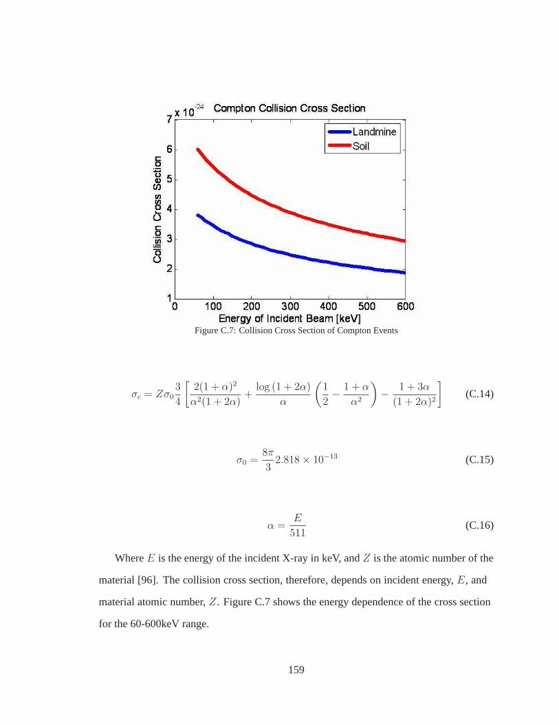
Figure C.7: Collision Cross Section of Compton Events

σc = Zσ03

4

[

2(1 + α)2

α2(1 + 2α)+

log (1 + 2α)

α

(

1

2− 1 + α

α2

)

− 1 + 3α

(1 + 2α)2

]

(C.14)

σ0 =8π

32.818 × 10−13 (C.15)

α =E

511(C.16)

WhereE is the energy of the incident X-ray in keV, andZ is the atomic number of the

material [96]. The collision cross section, therefore, depends on incident energy,E, and

material atomic number,Z. Figure C.7 shows the energy dependence of the cross section

for the 60-600keV range.

159

Note in Figure C.7 that the soil cross section is almost twice as high as the explosive

material of the landmine. This means that more backscattered x-rays will be generated by

the soil than by the explosive material. Images containing landmines will, therefore, have

lower signal-to-noise ratio than images without landmines.

C.4 X-ray Backscatter Conclusions

In this section the application of X-ray Backscatter Technology to the detection of

low-metal landmines has been explored. This approach makesuse of Compton Scattering

of x-rays and differing linear attenuation coefficients of explosive material and soil. The

difference arises from the atomic numbers (TNT: about7 and soil: about11) and the fact

that soil is significantly denser (TNT: 1.65gm3 and soil: 2.65 g

m3 ).

Investigation of the mathematical dependence of Compton andphoto-electric

attenuation shows that the best choice of x-ray energies is in the 300 to 1000keV region.

This is the region where Compton scattering is the dominant attenuation effect. A system

utilizing a set of collimated detectors is proposed. By employing a scanning scheme, the

system is able to acquire a 3D image set of the subsurface attenuation.

Because X-ray Backscatter keys on the material characteristics of the explosive

material, rather than the landmine casing, it is consideredan ideal technology for

non-metal cased (plastic) landmine detection.

160

BIBLIOGRAPHY

161

BIBLIOGRAPHY

[1] H. Ksienski, Y. Lin, and L. White, “Low-frequency approach to target identification,”Proceedings of the IEEE, vol. 63, pp. 1651–1659, 1975.

[2] M. Allen, J. Jauregui, and L. Hoff, “Fopen-sar detectionby direct use of simplescattering physics,” inProceedings of SPIE Algorithms for Synthetic Aperture RadarImagery II, (Orlando, FL), pp. 45–55, 1995.

[3] J. Gorman and J. Marble, “A low complexity multi-discriminant fopen targetscreener,” inProceedings of SPIE Algorithms for Synthetic Aperture Radar ImageryV, (Orlando, FL), pp. 307–317, 1998.

[4] C. Baum,Detection and Identification of Visually Obscured Targets. Bristol, PA:Taylor and Francis, 1988.

[5] J. Lee and S. Mudaliar, “Optimum polarizations in the bistatic scattering from layeredrandom media,”IEEE Trans. Geoscience and Remote Sensing, vol. 32, pp. 169–176,1994.

[6] A. Freundorfer and K. Iizuka, “A study on the scattering of radio waves from buriedspherical targets using the step frequency radar,”IEEE Trans. Geoscience andRemote Sensing, vol. 31, pp. 1253–1255, 1993.

[7] J. Ackenhusen, Q. Holmes, C. King, and J. Wright,Detection of Mines andMinefields. Ann Arbor, MI: Infrared Information Analysis Center, 2001.

[8] L. Carin, N. Geng, M. McClure, J. Sichina, and L. Nguyen, “Ultra-wide-bandsynthetic-aperture radar for mine-field detection,”IEEE Trans. Antennas andPropagation, vol. 41, pp. 18–33, 1999.

[9] W. Brown, “Synthetic aperture radar,”IEEE Trans. Aerospace and ElectronicSystems, vol. 3, pp. 217–229, 1967.

[10] W. Brown and L. Porcello, “Introduction to synthetic aperture radar,”IEEE Spectrum,pp. 52–62, 1969.

[11] D. Munson and R.Visentin, “A signal processing view of strip-mapping syntheticaperture radar,”IEEE Trans. Acoustics, Speech, and Signal Processing, vol. 37,pp. 2131–2147, 1989.

162

[12] R. Stewart,Methods of Satellite Oceonography. Berkeley, CA: University ofCalifornia Press, 1985.

[13] J. Johnson, P. Lucey, K. Horton, and E. Winter, “Spectral contrast differencesbetween field and laboratory infrared measurements of pristine and disturbed soils,”Remote Sensing of the Environment, vol. 64, pp. 33–46, 1998.

[14] M. Cherniakov and L. Donskoi, “Frequency band selectionof radars for buried objectdetection,”IEEE Trans. Geoscience and Remote Sensing, vol. 37, pp. 838–845, 1999.

[15] A. Hibbs and et al, “First year progress and test results,” in Proc. IEE. Detection ofAbandoned Landmines, pp. 138–141, 1998.

[16] D. Daniels,Surface Penetrating Radar. London: IEE, 2000.

[17] L. Riggs, J. Mooney, D. Lawrence, J. Broach, and A. Trang, “Identification ofmetallic mines using low frequency magnetic fields,” inProc. SPIE Int. Detectionand Remediation Technologies for Mines and Minelike Targets III, (Orlando, FL),pp. 146–157, 1998.

[18] C. Baum, “Singularity expansion method,”Proceedings of the IEEE, vol. 79,pp. 1481–1492, 1991.

[19] D. Hall and J. Llinas, “An introduction to multisensor data fusion,”Proceedings ofthe IEEE, vol. 1, pp. 6–22, 1997.

[20] L. Song, C. Yu, and Q. Liu, “Through-wall imaging (twi) byradar: 2-d tomographicresults and analyses,”IEEE Transactions on Geoscience and Remote Sensing,vol. 12, pp. 2793–2798, 2005.

[21] Q. Liu, Z. Zhang, and et.al., “Active microwave imagingi - 2-d forward and inversescattering methods,”IEEE Transactions on Microwave Theory and Techniques,vol. 50, pp. 123–133, 2002.

[22] Z. Zhang and Q. Liu, “Three-dimensional nonlinear image reconstruction formicrowave biomedical imaging,”IEEE Transactions on Biomedical Engineering,vol. 51, pp. 544–548, 2004.

[23] L. Song and Q. Liu, “Fast three-dimensional electromagnetic nonlinear inversion inlayered media with a novel scattering approximation,”Inverse Problems, vol. 20,pp. 171–194, 2004.

[24] C. Yu, L. Song, and Q. Liu, “Inversion of multi-frequencyexperimental datafor imaging complex objects by a dta-csi method,”Inverse Problems, vol. 21,pp. 165–178, 2004.

[25] S. Rao, D. Wilton, and A. Glisson, “Electromagnetic scattering by surfaces ofarbitrary shape,”IEEE Trans. Antenna Propag., vol. 30, pp. 409–418, 1992.

163

[26] P. Corona, A. D. Bonitatibus, G. Ferrara, and C. Gennarelli, “A very accurate modelfor backscattering by right angled dihedral corners,” inProceedings of the IEEEAntennas and Propagation Society International Symposium, pp. 1734–1737, 1990.

[27] J. Marble, D. Wilcox, and R. Mersereau, “Landmine signatures in ground penetratingradar,” inProc. SPIE Int. Detection and Remediation Technologies forMines andMinelike Targets VI, (Orlando, FL), pp. 720–729, 2001.

[28] X. Xiaoyin and E. Miller, “A statistical method to localize buried landmines from gprarray measurements,” inProc. SPIE Int. Detection and Remediation Technologies forMines and Minelike Targets VI, (Orlando, FL), pp. 742–753, 2001.

[29] J. Marble and A. Yagle, “Measuring landmine size and burial depth using groundpenetrating radar,” inProc. SPIE Int. Detection and Remediation Technologies forMines and Minelike Targets IX, (Orlando, FL), pp. 409–420, 2004.

[30] H. Anton,Calculus with Analytic Geometry. New York: John Wiley & Sons, 1984.

[31] Y. Nievergelt, “Fitting conics of specific types to data,” Linear Algebra and ItsApplications, vol. 378, pp. 1–30, 2004.

[32] J. Marble, D. Wilcox, and R. Mersereau, “Mine/uxo sensorphenomenology,” inProceedings 3rd Annual Federated Laboratory Symposium, (College Park, MD),pp. 317–322, 2000.

[33] A. Banos,Dipole radiation in the Presence of a Conducting Half-Space. London:Pergamon Press, 1966.

[34] T. Moon and W. Stirling,Mathematical Methods and Algorithms for SignalProcessing. Upper Saddle River, NJ: Prentice Hall, 2000.

[35] H. V. Trees,Detection, Estimation, and Modulation Theory. New York, NY: JohnWiley & Sons, 2001.

[36] C. Balanis,Advanced Engineering Electromagnetics. Hoboken, NJ: John Wiley &Sons, 1989.

[37] J. Marble, A. Yagle, and A. Hero, “Sensor management forlandmine detection,”in Proceedings of SPIE Detection and Remediation Technologies for Mines andMinelike Targets X, (Orlando, FL), pp. 1217–1228, 2005.

[38] T. Hastie, R. Tibshirani, and J. Friedman,The Elements of Statistical Learning. NewYork, NY: Springer-Verlag, 2001.

[39] W. Scott, K. Kim, G. Larson, and J. McClellan, “Combined seismic, radar, andinduction sensor for landmine detection,”IEEE Trans. Geoscience and RemoteSensing Society, vol. 3, pp. 1613–1616, 2004.

164

[40] P. Gao, L. Collins, L. Garber, N. Geng, and L. Carin, “Classification of landmine-likemetal targets using wideband electromagnetic induction,”IEEE Trans. Geoscienceand Remote Sensing Society, vol. 38, pp. 1352–1361, 2000.

[41] P. Gader, M. Mystkowski, and Y. Zhao, “Landmine detection with ground penetratingradar using hidden markov models,”IEEE Trans. Geoscience and Remote SensingSociety, vol. 38, pp. 1231–1244, 2001.

[42] S. Russel and P. Norvig,Artificial Intelligence A Modern Approach. Prentice Hall.

[43] W. Schmaedeke and K. Kastella, “Event-averaged maximum likelihood estimationand information-based sensor management,” inProceedings of SPIE, pp. 91–96,June 1994.

[44] K. Balaji, A. Hartemink, L. Carin, and M. M. Figueiredo, “Abayesian approach tojoint feature selection and classifier design,”IEEE Trans. on Pattern Analysis andMachine Intelligence, vol. 26, pp. 1105–1111, 2004.

[45] V. Krishnamurthy, “Algorithms for optimal schedulingand management of hiddenmarkov model sensors,”IEEE Trans. on Signal Processing, vol. 49, pp. 2893–2908,2001.

[46] C. Kreucher, E. Kastella, and A. Hero, “A bayesian approach to multiple targetdetection and tracking,”IEEE Trans. on Signal Processing, vol. 41, pp. 1396–1414,2005.

[47] A. Banos,Dipole radiation in the Presence of a Conducting Half-Space. London:Pergamon Press, 1966.

[48] J. Marble, A. Yagle, and G. Wakefield, “Physics derived basis pursuit in buried objectidentification using emi sensors,” inDetection and Remediation Technologies forMines and Minelike Targets X, (Orlando, FL), pp. 1151–1159, 2005.

[49] C. Wang and L. Collins, “Feature selection for physics model based objectdiscrimination,” inDetection and Remediation Technologies for Mines and MinelikeTargets X, (Orlando, FL), pp. 1200–1208, 2005.

[50] J. Marble, A. Yagle, and A. Hero, “Multimodal, adaptivelandmine detection usingemi and gpr,” inProceedings of SPIE Detection and Remediation Technologies forMines and Minelike Targets X, (Orlando, FL), pp. 1209–1216, 2005.

[51] L. Carin, N. Geng, M. McClure, Y. Dong, Z. Liu, J. He, J. Sichina, M. Ressler,L. Nguyen, and A. Sullivan, “Wide-area detection of land mines and unexplodedordnance,”Inverse Problems, vol. 18, pp. 575–609, 2002.

[52] X. Liao and L. Carin, “Application of the theory of optimal experiments to adaptiveelectromagnetic-induction sensing of buried targets,”IEEE Trans. on PatternAnalysis and Machine Intelligence, vol. 26, pp. 961–972, 2004.

165

[53] M. Kolba, P. Torrione, and L. Collins, “Information-based sensor managementfor landmine detection using multimodal sensors,” inDetection and RemediationTechnologies for Mines and Minelike Targets X, (Orlando, FL), pp. 1098–1107, 2005.

[54] D. Blatt and A. Hero, “From weighted classification to policy search,” inProc.of the Nineteenth Annual Conference on Neural Information Processing Systems,(Vancouver, BC), 2005.

[55] W. Scott, K. Kim, G. Larson, A. Gurbuz, and J. McClellan, “Combined seismic,radar, and induction sensor for landmine detection,” inProceedings of the IEEEInternational Geoscience and Remote Sensing Symposium, (Anchorage, AK),pp. 1613–1616, 2004.

[56] K. Kim and W. Scott, “An improved resistively-loaded vee dipole for ground-penetrating radar applications,” inProceedings of the IEEE Antennas andPropagation Society International Symposium, (Monterey, CA), pp. 2548–2551,2004.

[57] K. Kim and W. Scott, “A resistive linear antenna for ground penetrating radarapplications,” inDetection and Remediation Technologies for Mines and MinelikeTargets IX, (Orlando, FL), pp. 359–370, 2004.

[58] S. Twomey,Introduction to the Mathematics of Inversion in Remote Sensing andIndirect Measurements. Mineola, NY: Dover Publications, 1977.

[59] R. Raich and A. Hero, “Sparse image reconstruction for partially known blurfunctions,” inIEEE International Conference on Image Processing, (Atlanta, GA),pp. 637–640, 2006.

[60] J. Marble and A. Hero, “Iterative redeployment of illumination and sensing (iris):Application to stw-sar imaging,” inProc. of the 25th Army Science Conference,(Orlando, FL), 2006.

[61] L. Scharf,Statistical Signal Processing. Reading, MA: Addison-Wesley, 1991.

[62] C. Cafforio, C. Prati, and F. Rocca, “Sar data focusing usingseismic migrationtechniques,”IEEE Transactions on Aerospace and Electronic Systems, vol. 27,pp. 194–206, 1991.

[63] W. Carrara, R. Goodman, and R. Majewski,Spotlight Synthetic Aperture Radar.Boston: Artech House, 1995.

[64] M. Soumekh,Synthetic Aperture Radar Signal Processing. New York: Wiley-Interscience, 1999.

[65] R. Stolt, “Migration by fourier transform,”Geophysics, vol. 43, pp. 23–48, 1978.

[66] M. Ting, R. Raich, and A. Hero, “Sparse image reconstruction using sparse priors,” inIEEE International Conference on Image Processing, (Atlanta, GA), pp. 1261–1264,2006.

166

[67] M. Figueiredo and R. Nowak, “An em algorithm for wavelet-based imagerestoration,”IEEE Trans. Image Processing, vol. 12, pp. 906–916, 2003.

[68] A. Kong,Electromagnetic Wave Theory. Cambridge, MA: EMW Publishing, 2000.

[69] C. Balanis,Advanced Engineering Electromagnetics. Hoboken, NJ: John Wiley &Sons, 1989.

[70] E. Jordan and K. Balman,Electromagnetic Waves and Radiating Systems. EnglewoodCliffs, NJ: Prentice-Hall, 1968.

[71] W. Stutzman and G. Thiele,Antenna Design Theory. New York: John Wiley & Sons,1981.

[72] J. Marble and A. Yagle, “Measuring landmine size and burial depth using groundpenetrating radar,” inProc. SPIE Int. Detection and Remediation Technologies forMines and Minelike Targets IX, (Orlando, FL), pp. 409–420, 2004.

[73] F. Ulaby, R. Moore, and A. Fung,Microwave Remote Sensing (Vol.1). London:Addison-Wesley, 1981.

[74] H. Jakubowicz and S. Levin, “A simple exact method of 3-dmigration,”GeophysicalProspecting, vol. 31, pp. 34–56, 1983.

[75] Y. Yu, T. Yu, and L. Carin, “3d inverse scattering of a dielectric target embedded ina lossy half-space,”IEEE Transactions on Geoscience and Remote Sensing, vol. 5,pp. 957–973, 2004.

[76] J. Marble and A. O. Hero, “Phase distortion correction for see-through-the-wallradar imaging,” inProc. IEEE Int. Conf. on Image Processing, (Atlanta, GA),pp. 2333–2336, 2006.

[77] H. Haddar, S. Kusiak, and J. Sylvester, “The convex back-scattering support,”Journal of Applied Math, vol. 66, pp. 591–615, 2006.

[78] L. Potter and R. Moses, “Attributed scattering centers for sar atr,”IEEE Trans. ImageProc., vol. 6, pp. 79–91, 1997.

[79] P. Silverstein, O. Sands, and F. Garber, “Radar target classification and interpretationby means of structural descriptions of backscatter signals,” IEEE AES SystemsMagazine, vol. 6, pp. 3–7, 1991.

[80] R. Carriere and R. Moses, “High resolution radar target modeling using a modifiedprony estimator,”IEEE Trans. Antennas and Propagation, vol. 40, pp. 13–18, 1992.

[81] J. Marble and J. Gorman, “Performance comparison of phenomenology-basedfeatures to generic features for false alarm reduction in uwb sar imagery,” inProceedings of SPIE Algorithms for Synthetic Aperture Radar Imagery VI, (Orlando,FL), pp. 235–242, 1999.

167

[82] K. Kastella, “Discrimination gain to optimize classification,” IEEE Transactions onSystems, Man and Cybernetics-Part A: Systems and Humans, vol. 27, pp. 112–116,January 1997.

[83] C. Kreucher, K. Kastella, and A. O. Hero, “Multi-target sensor management usingalpha-divergence measures,” in3rd Workshop on Information Processing for SensorNetworks, (Palo Alto, CA), pp. 209–222, 2003.

[84] M. Yuan and Y. Lin, “Efficient empirical bayes variable selection and estimationin linear models,”Journal of the American Statistical Association, vol. 100,pp. 1215–1225, 2005.

[85] H. Libby, Introduction to Electromagnetic Nondestructive Test Methods. Malabar,FL: Robert E. Krieger Publishing Company, 1971.

[86] J. McNeill, Technical Note TN-7: Applications of Transient electromagneticTechniques. Mississuaga, ON: Geonics LTD, 1980.

[87] Y. Guo, Technical Report ST2-93-074: Electromagnetic Detection of an ObjectBuried in a Dissipative Medium. Laurel, MD: Johns Hopkins University / AppliedPhysics Laboratory, 1993.

[88] D. Hill and J. Wait, “The electromagnetic response of a buried sphere for burieddipole excitation,”Radio Science, vol. 8, pp. 813–818, 1973.

[89] Y. Guo, Technical Report ST2-94-020: Imaging Subsurface Objects by NearfieldElectromagnetic Holography. Laurel, MD: Johns Hopkins University / AppliedPhysics Laboratory, 1994.

[90] J. Lenz, “A review of magnetic sensors,”Proceedings of the IEEE, vol. 6,pp. 973–989, 1990.

[91] J. Campbell and A. Jacobs, “Detection of buried land mines by compton backscatterimaging,”Nuclear Science and Engineering, vol. 119, pp. 417–424, 1992.

[92] E. Dugan, A. Jacobs, Z. Su, L. Houssay, and D. Ekdahl, “Status of the xmis x-raybackscatter radiography landmine detection system,” inProceedings of the SPIEDetection and Remediation Technologies for Mines and Minelike Targets VIII,(Orlando, FL), pp. 34–44, 2003.

[93] A. Faust, R. Rothschild, and W. Heindl, “Development of a coded aperturebackscatter imager using the uc san diego hexis detector,” in Proceedings of theSPIE Detection and Remediation Technologies for Mines and Minelike Targets VIII,(Orlando, FL), pp. 95–106, 2003.

[94] J. McFee and A. Faust, “Defence r&d canada research on nuclear methods oflandmine detection,” inProceedings of the SPIE Detection and RemediationTechnologies for Mines and Minelike Targets VIII, (Orlando, FL), pp. 1–12, 2003.

168

[95] W. Niemann, S. Olesinski, and T. Thiele, “Detection of buried landmines with x-raybackscatter technology,”Non-destructive Testing, vol. 7, 2002.

[96] H. Barrett and W. Swindell,Radiological Imaging. New York: Academic Press,1981.

169