Environmental Science and Engineering

Advances in Wind Energy Conversion Technology

Bearbeitet vonMathew Sathyajith, Geeta Susan Philip

1. Auflage 2011. Buch. vIII, 216 S. HardcoverISBN 978 3 540 88257 2

Format (B x L): 15,5 x 23,5 cmGewicht: 535 g

Weitere Fachgebiete > Technik > Energietechnik, Elektrotechnik

Zu Inhaltsverzeichnis

schnell und portofrei erhältlich bei

Die Online-Fachbuchhandlung beck-shop.de ist spezialisiert auf Fachbücher, insbesondere Recht, Steuern und Wirtschaft.Im Sortiment finden Sie alle Medien (Bücher, Zeitschriften, CDs, eBooks, etc.) aller Verlage. Ergänzt wird das Programmdurch Services wie Neuerscheinungsdienst oder Zusammenstellungen von Büchern zu Sonderpreisen. Der Shop führt mehr

als 8 Millionen Produkte.

Analysis of Wind Regimesand Performance of Wind Turbines

Sathyajith Mathew, Geetha Susan Philip and Chee Ming Lim

With the present day’s energy crisis and growing environmental consciousness, theglobal perspective in energy conversion and consumption is shifting towardssustainable resources and technologies. This resulted in an appreciable increase inthe renewable energy installations in different part of the world. For example,Wind power could register an annual growth rate over 25% for the past 7 years,making it the fastest growing energy source in the world. The global wind powercapacity has crossed well above 160 GW today [1] and several Multi-Megawattprojects-both on shore and offshore-are in the pipeline. Hence, wind energy isgoing to be the major player in realizing our dream of meeting at least 20% of theglobal energy demand by new-renewables by 2020.

Assessing the wind energy potential at a candidate site and understanding how awind turbine would respond to the resource fluctuations are the initial steps in theplanning and development of a wind farm project. Energy yield from the WindEnergy Conversion System (WECS) at a given site depends on (1) strength anddistribution of wind spectra available at the site (2) performance characteristics ofthe wind turbine to be installed at the site and more importantly (3) the interactionbetween the wind spectra and the turbine under fluctuating conditions of the windregime.

Thus, models which integrate the wind resource as well as the turbine perfor-mance parameters are to be used in estimating the system performance. Based onthe above parameters, methods for assessing the available wind energy resource at

S. Mathew (&) and C. M. LimFaculty of Science, University of Brunei Darussalam, Jalan Tungku Link, Gadong,BE1410 Negra, Brunei Darussalame-mail: windbook@gmail.com

G. S. PhilipFaculty of Engineering, KAU, Kerala, India

S. Mathew and G. S. Philip (eds.), Advances in Wind EnergyConversion Technology, Environmental Science and Engineering,DOI: 10.1007/978-3-540-88258-9_2, � Springer-Verlag Berlin Heidelberg 2011

71

a candidate site and the performance expected from a wind turbine installed at thissite are presented in this chapter.

1 Wind Regime Characteristics

In this section we will discuss how the characteristics of the wind regimes can beincorporated in assessing the wind energy potential as well as estimating the outputfrom a wind energy conversion system.

1.1 Boundary Layer Effects

The first factor to be considered while estimating the wind resource and windturbine performance at a given site is the variations in wind velocity due to theboundary layer effect. Due to the frictional resistance offered by the earth surface(caused by roughness of the ground, vegetations etc.) to the wind flow, the windvelocity may vary significantly with the height above the ground. For example,wind profile at a site is shown in Fig. 1. Variations in the wind velocity with heightare quite evident in the figure. Thus, if the wind data available are not collectedfrom the hub height of the turbine, the data are to be corrected for the boundarylayer effect.

Ground resistance against the wind flow is represented by the roughness class orthe roughness height (Z0). The roughness height of a surface may be close to zero(surface of the sea) or even as high as 2 (town centers).

0

2

4

6

8

10

12

0 20 40 60 80

Distance from the ground, m

Win

d ve

loci

ty, m

/s

Fig. 1 Variation of windvelocity with height [2]

72 S. Mathew et al.

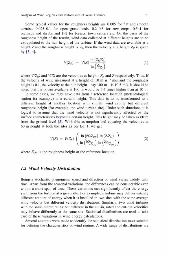
Some typical values for the roughness heights are 0.005 for flat and smoothterrains, 0.025–0.1 for open grass lands, 0.2–0.3 for row crops, 0.5–1 fororchards and shrubs and 1–2 for forests, town centers etc. On the basis of theroughness height of the terrain, wind data collected at different heights are to beextrapolated to the hub height of the turbine. If the wind data are available at aheight Z and the roughness height is Z0, then the velocity at a height ZR is givenby [3, 4].

VðZRÞ ¼ VðZÞln ZR=Z0� �

ln Z=Z0

� � ð1Þ

where V(ZR) and V(Z) are the velocities at heights ZR and Z respectively. Thus, ifthe velocity of wind measured at a height of 10 m is 7 m/s and the roughnessheight is 0.1, the velocity at the hub height—say 100 m—is 10.5 m/s. It should benoted that the power available at 100 m would be 3.4 times higher than at 10 m.

In some cases, we may have data from a reference location (meteorologicalstation for example) at a certain height. This data is to be transformed to adifferent height at another location with similar wind profile but differentroughness height (for example, the wind turbine site). Under such situations, it islogical to assume that the wind velocity is not significantly affected by thesurface characteristics beyond a certain height. This height may be taken as 60 mfrom the ground level [5]. With this assumption and equating the velocities at60 m height at both the sites as per Eq. 1, we get

VðZÞ ¼ VðZRÞln 60=ZOR

� �ln Z=ZO

� �

ln 60=ZO

� �ln ZR=ZOR

� �

0

@

1

A ð2Þ

where ZOR is the roughness height at the reference location.

1.2 Wind Velocity Distribution

Being a stochastic phenomena, speed and direction of wind varies widely withtime. Apart from the seasonal variations, the differences can be considerable evenwithin a short span of time. These variations can significantly affect the energyyield from the turbine at a given site. For example, a turbine may deliver entirelydifferent amount of energy when it is installed in two sites with the same averagewind velocity but different velocity distributions. Similarly, two wind turbineswith the same output rating but different in the cut-in, rated and cut-out velocitiesmay behave differently at the same site. Statistical distributions are used to takecare of these variations in wind energy calculations.

Several attempts were made to identify the statistical distribution most suitablefor defining the characteristics of wind regime. A wide range of distributions are

Analysis of Wind Regimes and Performance of Wind Turbines 73

being tried by the researchers. The Weibull distribution, which is a special case ofPierson class III distribution, is well accepted and commonly used for the windenergy analysis as it can represent the wind variations with an acceptable level ofaccuracy [6–9]. In some situations, Rayleigh distribution—which is a simplifiedform of Weibull distribution—is also being used. It is worth mentioning that someinnovative attempts are also been made by applying the Minimum Cross Entropy(MinxEnt) [10] and Maximum Entropy (ME) [11] principles in wind energyanalysis. However, a recent study comparing various statistical distributions inwind energy analysis has established the acceptability of Weibull distribution [9].Hence we will follow the Weibull distribution in our analysis.

The Weibull distribution can be defined by its probability density function f(V)and cumulative distribution function F(V) where:

f ðVÞ ¼ k

c

V

c

� �k�1

e� V=cð Þk ð3Þ

and

FðVÞ ¼Z

f ðVÞ dV ¼ 1� e� V=cð Þk ð4Þ

where k is the Weibull shape factor, c the scale factor and V is the velocity ofinterest. Here, f(V) represents the fraction of time (or probability) for whichthe wind blows with a velocity V and F(V) indicates the fraction of time(or probability) that the wind velocity is equal or lower than V.

From Eqs. 3 and 4, it is evident that k and c are the factors determining thenature of the wind spectra within a given regime. Effects k and c on the probabilitydensity and cumulative distribution of wind velocity are demonstrated using thewind data from three potential wind farm sites in Figs. 2 and 3. The site windvelocities are represented in Table 1.

Fig. 2 Effect of Weibullshape factor on theprobability density of windvelocity of some potentialsites

74 S. Mathew et al.

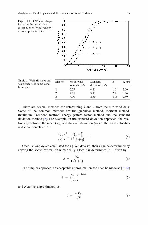
There are several methods for determining k and c from the site wind data.Some of the common methods are the graphical method, moment method,maximum likelihood method, energy pattern factor method and the standarddeviation method [2]. For example, in the standard deviation approach, the rela-tionship between the mean (Vm) and standard deviation (rV) of the wind velocitiesand k are correlated as

rV

Vm

� �2

¼C 1þ 2

k

� �

C2 1þ 1k

� � � 1 ð5Þ

Once Vm and rV are calculated for a given data set, then k can be determined bysolving the above expression numerically. Once k is determined, c is given by

c ¼ Vm

C 1þ 1k

� � ð6Þ

In a simpler approach, an acceptable approximation for k can be made as [7, 12]

k ¼ rV

Vm

� �� 1:090

ð7Þ

and c can be approximated as

c ¼ 2 Vmffiffiffipp ð8Þ

Fig. 3 Effect Weibull shapefactor on the cumulativedistribution of wind velocityat some potential sites

Table 1 Weibull shape andscale factors of some windfarm sites

Site no. Mean windvelocity, m/s

Standarddeviation, m/s

k c, m/s

1 6.79 4.11 1.6 7.662 7.75 3.11 2.7 8.743 6.99 2.50 3.06 7.89

Analysis of Wind Regimes and Performance of Wind Turbines 75

1.3 Energy Density

The power available in a wind stream of velocity V, per unit rotor area, is given by

PV ¼12

qa V3 ð9Þ

where PV is the power and qa is the density of air. The fraction of time for whichthis velocity V prevails in the regime is given by the probability density functionf(V). Thus, the energy contributed by V, per unit time and unit rotor area, isPV f(V). Hence, the total energy contributed by all possible velocities in the windregime, available for unit rotor area in unit time (that is energy density, ED) may beexpressed as

ED ¼Z1

0

PV f ðVÞ dV ð10Þ

Substituting for P(V) and f(V) in the above expression and simplifying, we get

ED ¼12qa

k

ck

Z1

0

Vðkþ2Þe� V=cð Þk dV ð11Þ

This can further be simplified as [2]

ED ¼32

qac3

kC

3k

� �ð12Þ

2 Velocity–Power Response of the Turbine

Power curve of a 2 MW pitch controlled wind turbine is shown in Fig. 4.The turbine has cut-in, rated and cut-out velocities 3.5, 13.5 and 25 m/s respec-tively. The given curve is a theoretical one and in practice we may observe thevelocity power variation in a rather scattered pattern.

In this curve, we can observe that the turbine has four distinct performanceregions.

1. For velocities from 0 to the cut-in (VI), the turbine does not yield any power.2. Between the cut-in and rated velocities (VI to VR), the power increases with the

wind velocity. Though, theoretically, this increase should be cubic in nature, inpractice it can be linear, quadratic, cubic and even higher powers and itscombinations, depending upon the design of the turbine.

3. From the rated to cut-out wind speed (VR to VO), the power is constant at therated power PR, irrespective of the change in wind velocity.

4. Beyond the cut-out velocity, the turbine is shut down due to safety reasons.

76 S. Mathew et al.

So, the wind turbine is ‘productive’ only between the velocities VI and VO. For anywind velocity between VI and VR, the power PV can generally be expressed as

PV ¼ aVn þ b ð13Þ

where a and b are constants and n is the velocity–power proportionality. Nowconsider the performance of the system at VI and VR. At VI, the power developedby the turbine is zero. Thus

aVnI þ b ¼ 0 ð14Þ

At VR power generated is PR. That is:

aVnR þ b ¼ PR ð15Þ

Solving Eqs. 14 and 15 for a and b and substituting in Eq. 13 yields

PV ¼ PRVn � Vn

I

VnR � Vn

I

� �ð16Þ

Above equation gives us the power response of the turbine between the cut-inand rated wind speeds. Obviously, the power between VR and VO is PR.

In the above expression, the major factor deciding the variations in power withvelocity in the cut-into rated wind speed region is n. Value of n differs from turbineto turbine, depending on the design features. For example, Fig. 5 comparesthe power responses of two commercial wind turbines in this performance region.The curves are derived from data available from the manufactures. It should benoted that, although both the turbines are of the same 2 MW rated capacity, theirpower responses in the ‘cut-into rated’ velocity region differ significantly.

For a specific turbine, n can be calculated from its power curve data, availablefrom the manufacturer. For example, the cut-in, rated and cut-out wind velocities

0

500

1000

1500

2000

2500

0 5 10 15 20 25 30

Velocity, m/s

Pow

er, W

VI VR VO

PR

Fig. 4 Theoretical powercurve of a 2 MW windturbine

Analysis of Wind Regimes and Performance of Wind Turbines 77

of the two turbines compared above are shown in Table 2. Putting these values inEq. 16 we get

PV T1½ � ¼ 2000 � Vn � 3n

12n � 3n

� �and PV T2½ � ¼ 2000 � Vn � 4n

16n � 4n

� �

where T1 and T2 represents the turbines 1 and 2 respectively. Solving the aboverelationship with the velocity power data for the turbines (available from the manu-facturer or obtained by digitizing the power curve) we can find out the value of n. Anystandard curve fitting package can be used for the solution. Following this method,n for the turbines T1 and T2 are 1.8 (R2 = 0.97) and 0.6 (R2 = 0.95) respectively.

Instantaneous values of wind velocity and corresponding power were recordedfrom a 225 kW wind turbine installed at a wind farm and are plotted in Fig. 6. Cut-in and rated wind velocities of this turbine are 3.5 and 14.5 m/s respectively.Scattered points represent the measured power where as the continuous line rep-resents the power computed using Eq. 16. Reasonable agreement could beobserved between measured and computed values.

3 The Energy Model

To estimate the energy generated by the turbine at a given site over a period, thepower characteristics of the turbine is to be integrated with the probabilities ofdifferent wind velocities expected at the site. For example, power curve of a wind

Table 2 Cut-in, rated andcut-out wind velocities of theturbines

Turbineno.

Cut-in velocity,m/s

Rated velocity,m/s

Cut-out velocity,m/s

1 3 12 282 4 16 25

Fig. 5 Variations in outputpower from cut-into cut-outvelocities for two windturbines of 2 MW ratedcapacity

78 S. Mathew et al.

turbine is shown in Fig. 7a whereas Fig. 7b presents the Weibull probabilitydensity function of a candidate site. In the wind regime, the fraction of energycontributed by any wind velocity V is the product of power corresponding to V inthe power curve, that is P(V) and the probability of V in the probability densitycurve, which is f(V). Thus, at this site, the total energy generated by the turbine E,over a period T, can be estimated by

E ¼ T

ZVo

Vi

PV f ðVÞ dV ð17Þ

As we have discussed, the power curve has two distinct productive regions—from VI to VR and VR to VO. Thus, let us take

E ¼ EIR þ ERO ð18Þ

Fig. 6 Field performance ofa 225 kW wind turbine

0

200

400

600

800

1000

1200

Wind velocity, m/s

Pow

er, k

W

(a)

0

0.02

0.04

0.06

0.08

0.1

0 10 20 30 0 10 20 30

Wind velocity, m/s

Prob

abili

ty(b)

P(V)

V

f(V)

V

Fig. 7 Integrating the power (a) and probability (b) curves to derive the energy yield

Analysis of Wind Regimes and Performance of Wind Turbines 79

where EIR and ERO are the energy yield corresponding to VI to VR and VR to VO

respectively. From the foregoing discussions, we have

EIR ¼ T

ZVR

Vi

PV f ðVÞ dV ð19Þ

and

ERO ¼ T PR

ZVO

VR

f ðVÞdV ð20Þ

Substituting for f(V) and P(V) from Eqs. 3 and 16 in Eq. 19, we get

EIR ¼ PR T

ZVR

VI

Vn � VnI

VnR � Vn

I

k

c

V

c

� �k�1

e� V=cð Þk dV

¼ PR T

VnR � Vn

I

� � ZVR

VI

Vn � VnI

� � k

c

V

c

� �k�1

e� V=cð Þk dV

ð21Þ

For simplifying the above expression and bringing it to a resolvable form, let usintroduce the variable X such that

X ¼ V

c

� �k

ð22Þ

Then,

dX ¼ k

c

V

c

� �k�1

and V ¼ cX1k ð23Þ

With Eq. 22, we have

XI ¼VI

c

� �k

; XR ¼VR

c

� �k

and XO ¼VO

c

� �k

ð24Þ

With this substitution, and simplification thereafter, EIR can be expressed as

EIR ¼PR T cn

VnR � Vn

Ið Þ

ZXR

XI

Xn=k e�X

dX

� PR T VnI

VnR � Vn

Ið Þ e�XI � e�XR� �

ð25Þ

80 S. Mathew et al.

Now consider the second performance region. From Eq. 20, ERO may berepresented as

ERO ¼ PR T

ZVO

VR

k

c

V

c

� �k�1

e� V=cð Þk dV ð26Þ

AsR

f ðVÞ dV ¼ FðVÞ, from Eqs. 4 and 16, the above equation can besimplified as

ERO ¼ T PR e�XR � e�XO� �

ð27Þ

The above expressions can be evaluated numerically.The capacity factor CF —which is the ratio of the energy actually produced by

the turbine to the energy that could have been produced by it, if the machine wouldhave operated at its rated power throughout the time period—is given by

CF ¼E

PR T¼ EIR þ ERO

PRTð28Þ

Thus,

CF ¼ cn

VnR � Vn

I

ZXR

XI

Xn=k e�X

dX

� VnI

VnR � Vn

I

e�XI � e�XR� �

þ e�XR � e�XO� �

ð29Þ

The energy model discussed above is validated with the field performance of a10 kW wind turbine [13] in Fig. 8. The turbine considered here has cut-in, ratedand cut-out wind speeds of 3.0, 13.5 and 25 m/s respectively. From the manu-facturer’s power curve, the velocity–power proportionality for the design was

0

10

20

30

40

50

60

70

1 3 5 7 9 11 13 15 17 19 21 23 25 27 29

Days

Ene

rgy,

kW

h

PredictedMeasured

Fig. 8 Comparison betweenestimated and measured dailyenergy yield from a 10 KWwind turbine

Analysis of Wind Regimes and Performance of Wind Turbines 81

found to be 2.16. It can be observed that the predicted performance closely followsthe measured values throughout the period.

4 Conclusion

A method for assessing the wind energy resource available at a potential wind farmsite has been presented in the above sections. Model for simulating the perfor-mance of wind turbines at a given site has also been discussed.

For example, the performances expected from the turbines given in Table 2,when installed at the sites described in Table 1 are compared in Fig. 9. Thoughboth the turbines have the same rated power of 2 MW, the first turbine is expectedto generate more energy from all the three sites. This is obvious as (1) the firstturbine has lower cut-in and higher cut-out velocities, making it capable ofexploiting a broader range of wind spectra available at the site (2) The first turbineshows better power response between the cut-into rated wind speeds as seen fromFig. 5.

The methods described above can be useful in the preliminary planning of windpower project. However, for a final investment decision, apart from a morerigorous technical analysis, economical and environmental dimensions of theproject should be investigated.

References

1. Renewable Energy World (2010) Global Wind Installations Boom, Up 31% in 2009.Retrieved from http://www.renewableenergyworld.com/rea/news/article/2010/02/global-wind-installations-boom-up-31-in-2009

2. Mathew S (2006) Wind Energy: Fundamentals, Resource Analysis and Economics. Springer-Verlag, Berlin Heidelberg

Fig. 9 Comparativeperformance of two 2 MWwind turbines in differentwind regimes

82 S. Mathew et al.

3. Machias AV, Skikos, GD (1992) Fuzzy risk index for wind sites. IEEE Transactions onEnergy Conversion 7(4):638–643

4. Mathew S, Pandey KP, Anil KV (2002) Analysis of wind regimes for energy estimation.Renewable Energy 25:381–399

5. Lysen EH (1983) Introduction to wind energy. CWD, Amersfoort, Netherlands6. Hennessey JP (1977) Some aspects of wind power statistics. J Applied Meteorology 16:

119-1287. Justus CG, Hargraves WR, Mikhail A, Graber D (1978) Methods of estimating wind speed

frequency distribution. J Applied Meteorology 17:350–3538. Stevens MJM, Smulders PT (1979) The estimation of parameters of the Weibull wind speed

distribution for wind energy utilization purposes. Wind Engineering 3(2):132–1459. Carta J A P. Ramírez P Velázquez S (2009) A review of wind speed probability distributions

used in wind energy analysis: Case studies in the Canary Islands. Renewable and SustainableEnergy Reviews 13(5):933–955

10. Yeliz MK, Ilhan U (2008) Analysis of wind speed distributions: Wind distribution functionderived from minimum cross entropy principles as better alternative to Weibull functionEnergy Conversion and Management 49(5):962–973

11. Meishen L, Xianguo Li (2005) MEP-type distribution function: a better alternative to Weibullfunction for wind speed distributions Renewable Energy 30(8):1221–1240

12. Boweden GJ, Barker PR, Shestopal VO, Twidell JW (1983) The Weibull distributionfunction and wind statistics. Wind Engineering 7:85–98

13. The Vermont Small-Scale Wind Energy Demonstration Program (2010) Retrieved fromhttp://www.vtwindprogram.org/performancedata/

Author Biography

Dr. Sathyajith Mathew is an Associate Professor at the Facultyof Engineering, KAU and holds a concurrent faculty position atthe University of Brunei Darussalam. He has more than 15 yearsof teaching, research and development experience on WindEnergy Conversion Systems in different parts of the world.Dr. Mathew has published extensively in this area of research.His recent book ‘‘Wind Energy: Fundamentals, Resource Anal-ysis and Economics’’ which is published by Springer has beenadopted as the text book for wind energy programmes in Uni-versities around the world. Dr. Mathew is also a freelance windenergy consultant and serves as a resource person to severalInternational Training Programmes on Wind Energy.

Analysis of Wind Regimes and Performance of Wind Turbines 83