adventures in radio astronomy instrumentation...
TRANSCRIPT

Adventures in Radio Astronomy
Instrumentation and Signal Processing
by
Peter Leonard McMahon
Submitted to the Department of Electrical Engineering
in partial fulfillment of the requirements for the degree of
Master of Science in Electrical Engineering
at the
University of Cape Town
July 2008
Supervisor: Professor Michael Inggs
Co-supervisors:
Dr Dan Werthimer, CASPER1, University of California, Berkeley
Dr Alan Langman, Karoo Array Telescope
1Center for Astronomy Signal Processing and Electronics Research
arX
iv:1
109.
0416
v1 [
astr
o-ph
.IM
] 2
Sep
201
1

Abstract
This thesis describes the design and implementation of several instruments for digi-
tizing and processing analogue astronomical signals collected using radio telescopes.
Modern radio telescopes have significant digital signal processing demands that
are typically best met using custom processing engines implemented in Field Pro-
grammable Gate Arrays. These demands essentially stem from the ever-larger ana-
logue bandwidths that astronomers wish to observe, resulting in large data volumes
that need to be processed in real time.
We focused on the development of spectrometers for enabling improved pulsar2 sci-
ence on the Allen Telescope Array, the Hartebeesthoek Radio Observatory telescope,
the Nancay Radio Telescope, and the Parkes Radio Telescope. We also present work
that we conducted on the development of real-time pulsar timing instrumentation.
All the work described in this thesis was carried out using generic astronomy pro-
cessing tools and hardware developed by the Center for Astronomy Signal Processing
and Electronics Research (CASPER) at the University of California, Berkeley. We
successfully deployed to several telescopes instruments that were built solely with
CASPER technology, which has helped to validate the approach to developing radio
astronomy instruments that CASPER advocates.
2Pulsars are rapidly rotating neutron stars that emit periodic broad band electromagnetic radi-
ation.

Plagiarism Declaration
I know the meaning of plagiarism and declare that all the work in this document,
save for that which is properly acknowledged, is my own.
i

Contents
1 Introduction 1
1.1 Background . . . . . . . . . . . . . . . . . . . . . . . . . . . . . . . . 1
1.2 Objectives . . . . . . . . . . . . . . . . . . . . . . . . . . . . . . . . . 2
1.2.1 Development of Spectrometers for Incoherent Dedispersion Ap-
plications . . . . . . . . . . . . . . . . . . . . . . . . . . . . . 2
1.2.2 Development of Spectrometers for Coherent Dedispersion Ap-
plications . . . . . . . . . . . . . . . . . . . . . . . . . . . . . 3
1.3 Thesis Outline and Summary . . . . . . . . . . . . . . . . . . . . . . 3
1.4 Contributions . . . . . . . . . . . . . . . . . . . . . . . . . . . . . . . 4
2 Background 7
2.1 An Engineer’s View of Radio Astronomy and Instrumentation . . . . 7
2.2 Single Antenna Radio Astronomy . . . . . . . . . . . . . . . . . . . . 8
2.2.1 Radio Telescope Arrays . . . . . . . . . . . . . . . . . . . . . . 10
2.3 Pulsar Science . . . . . . . . . . . . . . . . . . . . . . . . . . . . . . . 12
2.4 Instrumentation for Pulsar Science . . . . . . . . . . . . . . . . . . . 17
2.5 CASPER . . . . . . . . . . . . . . . . . . . . . . . . . . . . . . . . . 23
2.5.1 The CASPER Approach . . . . . . . . . . . . . . . . . . . . . 23
2.5.2 CASPER Hardware . . . . . . . . . . . . . . . . . . . . . . . . 24
2.5.3 CASPER Toolflow and Libraries . . . . . . . . . . . . . . . . . 26
3 The Fly’s Eye: Instrumentation for the Detection of Millisecond
Radio Pulses 28
3.1 Science Motivation . . . . . . . . . . . . . . . . . . . . . . . . . . . . 28
3.2 Searching for Bright Pulses with the ATA . . . . . . . . . . . . . . . 30
3.3 System Architecture . . . . . . . . . . . . . . . . . . . . . . . . . . . 33
3.4 A 210MHz Quad Spectrometer . . . . . . . . . . . . . . . . . . . . . 36
ii
3.5 Observing Software . . . . . . . . . . . . . . . . . . . . . . . . . . . . 40
3.6 Offline Processing to Detect Transients . . . . . . . . . . . . . . . . . 43
3.6.1 Equalization . . . . . . . . . . . . . . . . . . . . . . . . . . . . 43
3.6.2 RFI Rejection . . . . . . . . . . . . . . . . . . . . . . . . . . . 45
3.7 Test Results . . . . . . . . . . . . . . . . . . . . . . . . . . . . . . . . 46
3.7.1 Detection of the Hydrogen Spectral Line . . . . . . . . . . . . 46
3.7.2 Detection of Pulses from PSR B0329+54 . . . . . . . . . . . . 47
3.7.3 Detection of Giant Pulses from the Crab Nebula . . . . . . . . 48
4 Fast-readout 10GbE Spectrometers for Incoherent Dedispersion Ap-
plications 53
4.1 The Parkes and HartRAO Pulsar Spectrometers . . . . . . . . . . . . 54
4.1.1 A 400MHz Fast-readout Dual Power Spectrometer for Parkes . 54
4.1.2 A 400MHz Fast-readout Dual “Full Stokes” Spectrometer for
HartRAO . . . . . . . . . . . . . . . . . . . . . . . . . . . . . 58
4.1.3 Test Results . . . . . . . . . . . . . . . . . . . . . . . . . . . . 58
4.2 The Berkeley ATA Pulsar Processor . . . . . . . . . . . . . . . . . . . 61
4.2.1 Overall Architecture . . . . . . . . . . . . . . . . . . . . . . . 62
4.2.2 A 105MHz Fast-readout Dual Spectrometer with Digital Beam-
former Interface . . . . . . . . . . . . . . . . . . . . . . . . . . 65
4.2.3 Test Results . . . . . . . . . . . . . . . . . . . . . . . . . . . . 66
5 A Load Balanced Spectrometer for Coherent Dedispersion Applica-
tions 70
5.1 Overall Architecture . . . . . . . . . . . . . . . . . . . . . . . . . . . 70
5.2 A Static Load Balancing 400MHz Dual Spectrometer . . . . . . . . . 72
5.3 Test Results . . . . . . . . . . . . . . . . . . . . . . . . . . . . . . . . 76
6 Conclusions 78
6.1 Results Obtained . . . . . . . . . . . . . . . . . . . . . . . . . . . . . 78
6.2 Future Work . . . . . . . . . . . . . . . . . . . . . . . . . . . . . . . . 79
A Investigation into Building a FPGA-Based Real-Time Coherent Dedis-
persion System 81
A.1 Coherent Dedispersion on Compute Clusters . . . . . . . . . . . . . . 82
iii

A.2 Coherent Dedispersion on CASPER Reconfigurable Computing Plat-
forms . . . . . . . . . . . . . . . . . . . . . . . . . . . . . . . . . . . . 84
A.2.1 BEE2 . . . . . . . . . . . . . . . . . . . . . . . . . . . . . . . 85
A.2.2 ROACH . . . . . . . . . . . . . . . . . . . . . . . . . . . . . . 88
A.3 Conclusions . . . . . . . . . . . . . . . . . . . . . . . . . . . . . . . . 88
B Derivation of Expected Noise Correlation Results 90
B.1 Introduction . . . . . . . . . . . . . . . . . . . . . . . . . . . . . . . . 90
B.2 A Mathematical Description of a Full Stokes Spectrometer . . . . . . 91
B.3 The Distribution of the Fourier Coefficients of Real Gaussian-distributed
Time-domain Data . . . . . . . . . . . . . . . . . . . . . . . . . . . . 92
B.4 The Statistics of the Spectrometer Outputs Σ1, Σ2, Σ3 and Σ4 . . . . 94
B.4.1 The Mean and Variance of Σ1 and Σ2 . . . . . . . . . . . . . . 94
B.4.2 The Mean and Variance of Σ3 and Σ4 . . . . . . . . . . . . . . 95
C User Guide for the Parkes Spectrometer 97
C.1 Introduction . . . . . . . . . . . . . . . . . . . . . . . . . . . . . . . . 97
C.2 Hardware Setup . . . . . . . . . . . . . . . . . . . . . . . . . . . . . . 98
C.3 Software Configuration . . . . . . . . . . . . . . . . . . . . . . . . . . 100
C.3.1 Connectivity Settings . . . . . . . . . . . . . . . . . . . . . . . 100
C.3.2 Spectrometer Data Settings . . . . . . . . . . . . . . . . . . . 103
C.4 10GbE Packet Format . . . . . . . . . . . . . . . . . . . . . . . . . . 108
C.4.1 Receiving 10GbE/1GbE Packets on the Data Recorder Computer109
C.5 Precise Timing using ARM and 1PPS . . . . . . . . . . . . . . . . . . 110
iv

List of Figures
2.1 A Two-Element Phased Array. . . . . . . . . . . . . . . . . . . . . . . 11
2.2 Time series data taken at Arecibo showing individual pulses from PSR
B0301+19. . . . . . . . . . . . . . . . . . . . . . . . . . . . . . . . . . 13
2.3 Pulse profile of PSR J0437-4715. . . . . . . . . . . . . . . . . . . . . . 15
2.4 Frequency-Phase Plot of Dispersion of PSR B1356-60. . . . . . . . . . 16
2.5 Pulse profiles of PSR B1937+21 showing the effect of coherent versus
incoherent dedispersion. . . . . . . . . . . . . . . . . . . . . . . . . . 18
2.6 Data Flow in a Spectrometer for Incoherent Dedispersion Applications. 21
2.7 Data Flow in a Spectrometer for Coherent Dedispersion Applications. 22
2.8 IBOB Block Diagram. . . . . . . . . . . . . . . . . . . . . . . . . . . 25
3.1 A Single Bright Pulse of Extragalactic Origin. . . . . . . . . . . . . . 29
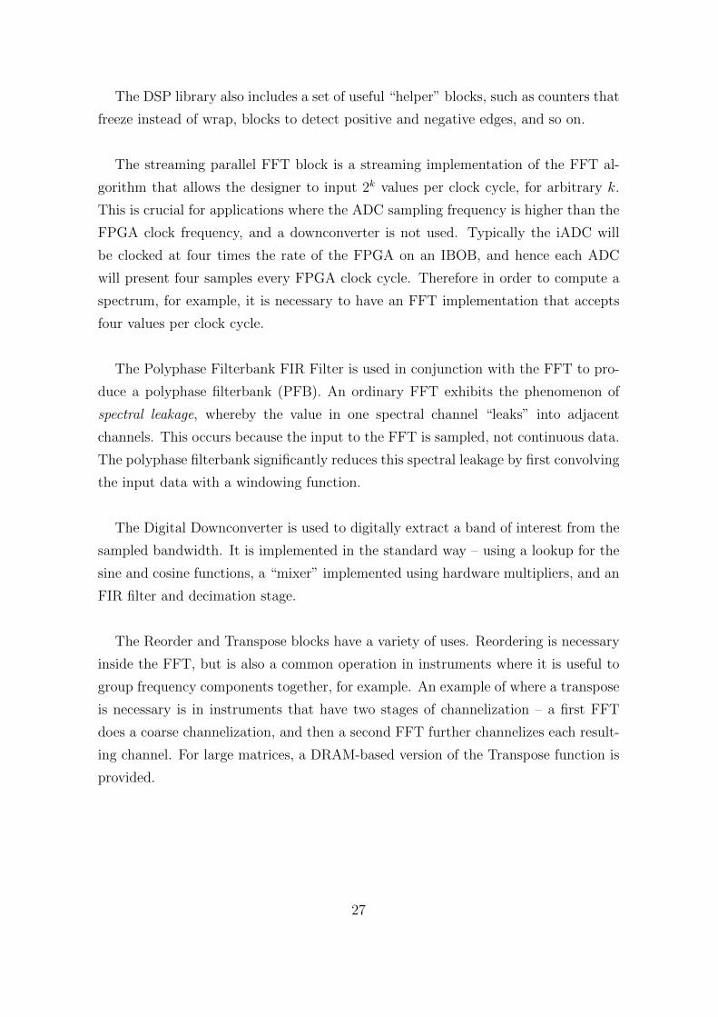
3.2 Beam Pattern from the Parkes Pulsar Survey. . . . . . . . . . . . . . 30
3.3 A hexagonal packing beam pattern for 42 antennas at the ATA. . . . 31
3.4 Sky coverage over 24 hours for 42 antennas at the ATA. . . . . . . . . 32
3.5 Fly’s Eye System Architecture. . . . . . . . . . . . . . . . . . . . . . 33
3.6 Fly’s Eye Rack at the ATA. . . . . . . . . . . . . . . . . . . . . . . . 34
3.7 Signal path for the Fly’s Eye Experiment at the ATA. . . . . . . . . . 35
3.8 A Quad Spectrometer for the Fly’s Eye. . . . . . . . . . . . . . . . . 38
3.9 The Output Stage of the Fly’s Eye Quad Spectrometer. . . . . . . . . 39
3.10 PowerPC-FPGA Interface of the Fly’s Eye Quad Spectrometer. . . . 40
3.11 Fly’s Eye Control Architecture. . . . . . . . . . . . . . . . . . . . . . 41
3.12 Fly’s Eye Control Script Flow. . . . . . . . . . . . . . . . . . . . . . . 42
3.13 Fly’s Eye Cluster Processing Chain. . . . . . . . . . . . . . . . . . . . 44
3.14 Fly’s Eye Spectra from a Single IBOB. . . . . . . . . . . . . . . . . . 47
3.15 Pulse Profile of PSR B0329+54 obtained using the Fly’s Eye. . . . . . 49
3.16 Pulse profiles calculated for all 44 independent spectrometers. . . . . 50
v

3.17 Crab Pulsar Observation Diagnostics. . . . . . . . . . . . . . . . . . . 51
3.18 A Giant Pulse from the Pulsar in the Crab Nebula. . . . . . . . . . . 52
4.1 Parspec: a Dual Power Spectrometer for the Parkes Radio Telescope. 56
4.2 Time Stamping Logic. . . . . . . . . . . . . . . . . . . . . . . . . . . 57
4.3 A Dual “Full Stokes” Spectrometer for the Hartebeesthoek Radio As-
tronomy Observatory. . . . . . . . . . . . . . . . . . . . . . . . . . . . 59
4.4 Pulse profile of PSR B1937+21 obtained using the Parkes Spectrometer
at NRAO Green Bank. . . . . . . . . . . . . . . . . . . . . . . . . . . 60
4.5 Pulse profile and diagnostics of PSR J1028-5820 obtained using the
Parkes Spectrometer with the Parkes Radio Telescope. . . . . . . . . 61
4.6 Pulse profile of PSR B0833-45 (Vela) obtained using the HartRAO
Spectrometer. . . . . . . . . . . . . . . . . . . . . . . . . . . . . . . . 62
4.7 BAPP Architecture. . . . . . . . . . . . . . . . . . . . . . . . . . . . 63
4.8 Signal Flow for BAPP at the ATA. . . . . . . . . . . . . . . . . . . . 64
4.9 BAPP Installation. . . . . . . . . . . . . . . . . . . . . . . . . . . . . 65
4.10 The Berkeley ATA Pulsar Processor Spectrometer: a 105MHz Fast-
readout Dual Spectrometer. . . . . . . . . . . . . . . . . . . . . . . . 67
4.11 Detection of Individual Pulses from PSR B0329+54. Image courtesy
Joeri van Leeuwen. (Figure compressed to meet arXiv file size require-
ments.) . . . . . . . . . . . . . . . . . . . . . . . . . . . . . . . . . . . 69
5.1 System Architecture for a Coherent Dedispersion Pulsar Study. . . . 71
5.2 A Fast-readout Dual Spectrometer with “raw complex voltage” output. 73
5.3 The 10GbE Output Stage. . . . . . . . . . . . . . . . . . . . . . . . . 74
A.1 A High-Level BEE2 Architecture for a Real-Time Coherent Dedisper-
sion System. . . . . . . . . . . . . . . . . . . . . . . . . . . . . . . . . 86
A.2 A Corner Turner for a Real-Time Coherent Dedispersion System. . . 87
C.1 IBOB with labeled connectors and ports. . . . . . . . . . . . . . . . . 99
C.2 Block diagram of the Parspec FPGA design. The register inputs to
the second spectrometer are shown. . . . . . . . . . . . . . . . . . . . 116
vi

List of Tables
2.1 Pulsars Useful for Instrument Tests. . . . . . . . . . . . . . . . . . . . 23
A.1 Chirp Function and FFT Lengths Required for Coherent Dedispersion. 83
C.1 Parkes Spectrometer Specifications Sheet . . . . . . . . . . . . . . . . 113
vii

To my teachers.
viii

Acknowledgements
An oft-used introduction to thesis acknowledgements is that there is an irony that
somehow research papers list as authors anyone who contributes, whereas their far
more lengthy brethren, theses, unfairly list only one author when in fact even greater
debt is owed to many people. This is particularly apt in my case. This thesis would
quite literally not have been possible without the assistance of many people, and
would be considerably worse off were it not for the help of many more. I have relied
heavily on the great generosity of my collaborators and the science and engineering
communities at large.
The first pivotal figure in the creation of this thesis is Professor Inggs, who intro-
duced me to Dr Alan Langman at the Karoo Array Telescope in September 2006, on
the completion of my undergraduate project. Had that meeting not taken place, I
likely wouldn’t have undertaken this thesis. Prof. Inggs has been terrific in taking
care of funding and in creating opportunities for me to collaborate with other groups,
and has in this role been a great enabler for my research.
Dr Alan Langman at KAT has given me many hours of excellent advice, but most
importantly, he provided me with the opportunity to spend 11 months with his col-
laborators in the CASPER3 group at Berkeley. I hope that his faith in me has paid
off in some small measure. The bulk of the work reported in this thesis was done
while I was at Berkeley, so Alan’s support of my visit made it possible for me to do
the work that you can see presented to you here shortly.
Dan Werthimer at CASPER is the third individual to whom this thesis owes its
existence, and hence to whom I am extremely grateful. Dan generously agreed to
allow Jason Manley and I to join his group despite our lack of credentials and experi-
ence. He then proceeded to patiently teach me many of the fundamentals of building
analogue/digital instruments that I should have known, but didn’t, to get me to a
point where I could carry out the projects that are described in these pages. Dan is
an outstanding mentor and supervisor, and I think it’s fairly safe to say that because
of him I learnt more in my year in Berkeley that I’ve learnt in any year prior. Dan
3Center for Astronomy Signal Processing and Electronics Research, University of California,
Berkeley
ix

provided a superb combination of direction when I needed it and freedom for me to
tinker otherwise, and this supervision style let me both learn and be semi-productive4.
I also owe Dan a debt of gratitude for his willingness to make connections for me
with his collaborators when I needed project ideas or help. Dan’s extensive network
of contacts made a massive difference in my ability to solve problems that I encoun-
tered. In this section I will try to thank all the people who have helped me over
the past year and a half, but it is a great many, so please forgive me if I make any
omissions.
At Berkeley, I was privileged to work with Prof. Don Backer and Dr Joeri van
Leeuwen on instrumentation for pulsar science, and particularly a spectrometer for
the Allen Telescope Array. I benefited greatly from the many discussions Don and
I had; Don was an invaluable source of practical knowledge and techniques to meet
challenges that routinely crop up in the development of pulsar instrumentation. Joeri
was my day-to-day contact with the science user community, and he did an excellent
job of keeping me focused on building “something people can use”. He also put up
with my stream of questions about pulsars as well as pulsar signal processing, so what
little I know of pulsar science and the techniques for finding and timing pulsars I owe
mostly to Joeri.
Dr Melvyn Wright and Prof. Geoffrey Bower, also from the Astronomy Depart-
ment, both provided very useful advice, and kindly supported the efforts I was in-
volved in to deploy instruments to the ATA.
Oren Milgrome, Dave MacMahon, Matt Dexter and Colby Kraybill from the Berke-
ley Radio Astronomy Lab5 (RAL) provided invaluable technical help that cumula-
tively probably saved me a couple of months. They also provided a great deal of
entertainment during debugging sessions in the RAL basement.
Dr Rick Forster, the ATA’s resident scientist at the Hat Creek Radio Observatory,
was extremely helpful, and cheerfully reset servers for us in the middle of the night,
4The “semi-” caveat is required purely due to my inadequacies!5RAL is responsible for much of the digital electronics at the ATA, amongst many other aspects
of the ATA’s design and development.
x

moved disks around, and otherwise made maintaining our instruments at the ATA
relatively painless. I’d also like to thank Rick and the rest of the staff at HCRO for
all their help and hospitality during our site visits.
Dr Billy Barott, who is now an assistant professor at Embry-Riddle Aeronautical
University, co-built the ATA beamformer, on which one of my instruments relies. Billy
provided support to Joeri and I during the ATA pulsar machine planning phases, and
while we were learning how to use the beamformer. Without his and Oren’s help, we
would undoubtedly have had great difficulty getting the Berkeley ATA Pulsar Pro-
cessor (BAPP) system to work.
I’d like to thank Nancy Wang at Berkeley and Dr Rachael Padman at the Univer-
sity of Cambridge for providing help with some Stokes parameter statistics questions
I had (thanks also to Mel for putting me in touch with Rachael).
CASPER’s chief engineer, Henry Chen, provided many hours of excellent advice
and free digital design tuition. I can’t thank him enough. Without his help, I would
have gone nowhere fast.
I entered the CASPER group as Aaron Parsons was leaving for Puerto Rico, but I
managed to get from him an excellent introduction to the CASPER DSP libraries, of
which he was the primary developer. Aaron did an excellent job with the libraries, and
it’s partially a testament to his workmanship that so many people are now using them.
I gratefully acknowledge Dr Chen Chang and Pierre-Yves Droz for their work on
developing the BEE2 and the Simulink toolflow. They had both left Berkeley before
my tenure, but their work lives on.
I had an excellent time in Berkeley courtesy of the students at the Berkeley Wire-
less Research Center and CASPER. I also benefitted from their help, and learnt from
them all. Ben Blackman, Daniel Chapman, Terry Filiba, Griffin Foster, Greg Gibel-
ing, Alex Krasnov, Vinayak Nagpal, Arash Parsa, Andrew Siemion, Mark Wagner,
and my South African travel partner, Jason Manley, all contributed towards this
thesis in meaningful ways. I also spent many fun non-work-related evenings with
CASPERites – thank you all!
xi

The staff at the BWRC also provided excellent help and support – I’d like to
thank Brian Richards, Fred Burghardt, Dan Burke, Sue Mellers, Kevin Zimmerman
and Brad Krebs. I also benefited greatly from many lunchtime discussions with Brian
and Dan in particular.
It was a pleasure to work with Glenn Jones from Caltech. Glenn has been an
excellent collaborator, and has acted as a very patient sounding-board for ideas on
spectrometer system design. He also provided many library blocks that I have made
use of in my projects. I had a useful and fun6 trip to NRAO in Green Bank, WV,
with Glenn as well.
John Ford, Randy McCullough and Dr Glen Langston at NRAO Green Bank have
been fun to work with, and I’d like to thank John especially for inviting me to his
GUPPi pulsar workshop in 2007. I had interesting discussions with Dr Scott Ran-
som, Dr Paul Demorest, Prof. Maura McLaughlin and Prof. Dunc Lorimer at that
meeting. I’d like to thank Maura in particular for help she subsequently gave me with
sigproc, and Paul for his helpful advice on coherent dedispersion systems.
Glen Langston at NRAO, and Andrew Jameson and Willem van Straten at the
Swinburne University of Technology kindly beta-tested the Parkes Spectrometer de-
sign (at Green Bank, and on the Parkes Radio Telescope, respectively). Glen has also
been a valuable source of design ideas and techniques.
I’d like to thank Prof. Roy Booth, Dr Michael Gaylard, Dr Jonathan Quick and
Sarah Buchner at the Hartebeesthoek Radio Astronomy Observatory for supporting
my efforts to install and test a spectrometer on their main telescope. Jon and Sarah
in particular deserve mention for all the effort they put into getting the spectrometer
set up.
I had several very helpful e-mail exchanges with Dr Ismael Cognard and Dr Gilles
Theureau from CNRS Orleans about the signals and systems available at the Nancay
Radio Telescope, and about Ismael’s work on GPU implementations of coherent dedis-
6Based on a visit there with Glenn, I can highly recommend the Western Sizzlin’ Wood Grill
Buffet in Harrisonburg, VA, to anyone making the trip from the East.
xii

persion.
I was fortunate to have thesis examiners who improved the quality of this thesis
through their careful reading of it, and their subsequent comments. I am grateful to
Prof. Michael Inggs, Dr Alan Langman and Prof. Matthew Bailes for the suggestions
in their examination reports.
I’d like to thank Profs. Birgitta Whaley and Yun Song for allowing me to sit in
on their classes at Berkeley, lest I forget what attending lectures is like. I had a fun
time learning about quantum computing and population genetics from them.
Dan’s wife, Mary-Kate, and Joeri’s wife, Annemieke, both kindly shared their
homes with me, and provided Jason and I with a respite from the International
House’s dining hall delights.
Prior to going to Berkeley, I spent a couple of months at EPCC7 at the University
of Edinburgh. I’m grateful to Prof. Inggs and Dr Mark Parsons at EPCC for facil-
itating this visit, and to Dr Rob Baxter and James Perry for teaching me all about
the “Maxwell” reconfigurable supercomputer. I had a great time in Edinburgh with
my fellow traveler, Drew “That’s a Girl’s Name8” Woods. Dr Mario Antonioletti
provided entertainment at the office and at Wednesday “Pints” at KB House. Our
European flatmates, Arturo, Gara, Heinreich, Leonardo, Luca, Mario S., Milda and
Steffen added greatly to the experience.
As part of my training on Maxwell, I spent a week in Bristol at Nallatech’s UK
Design Office with Drew. Allan Cantle went out of his way to arrange this for us,
and we had many useful discussions with Robin Bruce, Dan Denning, Gildas Genest
and Eric Lord while we were there.
I’d like to thank Dr Mike Keith for a useful discussion I had with him at the
Manchester Reconfigurable Supercomputing Conference during my visit to the UK,
on his work with Jodrell Bank to do pulsar data processing using grid technology.
7Formerly “EPCC” stood for “Edinburgh Parallel Computing Centre”.8Mario Antonioletti refused to believe that “Drew” can be a masculine name, and Joeri van
Leeuwen was confused by it too.
xiii

During my Masters I’ve had outstanding administrative support from Regine Lord
at RRSG, Lee-Ann Poggenpoel and Niesa Burgher at KAT, Catherine Inglis at Ed-
inburgh, Tom Boot at BWRC and Stacey-Lee Harrison at the UCT Postgraduate
Funding Office.
Alan Langman and Andrew Siemion kindly proof-read this thesis and caught sev-
eral errors, hence helping me avoid considerable embarrassment. Needless to say, any
remaining errors are my own fault.
I thank my friends and family for their support.
The work in this thesis has been generously supported by the National Research
Foundation in the form of a KAT Masters bursary, an NRF M.Sc. Scarce Skills
Prestigious SET bursary, and KAT travel funding. I also received UCT Postgraduate
Funding Office support, and the CASPER group is supported by U.S. National Science
Foundation Grant No. 0619596 and Infrastructure Grant No. 0403427. I would also
like to acknowledge Xilinx for donating the FPGAs that I used, and Kees Vissers
from Xilinx, for his continued support.
xiv

Chapter 1
Introduction
This thesis presents the designs of several instruments developed for radio astronomy
applications using generic reconfigurable computing hardware and toolflows. In this
introduction, we provide a brief background and motivation, provide details of the
objectives of the thesis, and outline the contents of the thesis.
1.1 Background
Radio astronomy is concerned with the study of the universe using radio frequency
electromagnetic signals that are emitted as a result of physical processes and can be
detected on or near1 Earth using radio receivers.
Digital signal processing technology has enabled great advances in radio astronomy,
but astronomers have an insatiable appetite for digital signal processing capacity, and
the instruments described in this thesis have primarily helped to increase the band-
width that can be observed. A simple implication of Nyquist’s sampling theorem to
DSP is that in order to increase the observable bandwidth, it is necessary to propor-
tionately increase the sampling rate, and hence the data rate increases. This increased
data rate typically necessitates the development of hardware that can firstly sample
at the required rate and secondly process the data in real time2.
1Radio telescopes can be mounted on spacecraft, and there are proposals for building radio
telescopes on Earth’s moon (to reduce radio frequency interference).2The requirement of real time processing is a result of the high sampling rates that are used;
it is not feasible to store unprocessed data for any significant length of time. For example, if an
astronomer wishes to observe for 10 hours, and the bandwidth is 1GHz, with 8-bit sampling the
data rate will be 2 GBytes/sec, and hence approximately 70 TBytes of storage would be required.
1

The Center for Astronomy Signal Processing and Electronics Research (CASPER)
at the University of California, Berkeley, has developed a common set of hardware,
tools, libraries and processing software [13] that are intended to allow for the develop-
ment of a wide range of astronomy signal processing instruments. This development
has been an effort to promote reuse of hardware, gateware3 and software whereever
possible, whereas in the past most radio astronomy instruments have been devel-
oped from scratch, with very little reuse between projects at a single observatory, let
alone between teams at different observatories. A partial explanation for this lack of
reuse in the past is that most projects have used custom interfaces that are specific
to a particular observatory at best, and often to an individual project. CASPER
advocates the use of industry standard interconnect and interface technologies, par-
ticularly XAUI and 100Mbit, 1Gbit and 10Gbit Ethernet. The use of these standard
interfaces not only makes it relatively simple to interface different instruments built
using CASPER hardware, but also allows for easy interfacing with external devices
such as control computers and data recorder computers.
1.2 Objectives
In this thesis we describe the design and development of several instruments, and the
preliminary results from their deployments that verify their functionality. Broadly
the development and investigations we carried out were as follows:
1.2.1 Development of Spectrometers for Incoherent Dedis-
persion Applications
We were tasked with the development of fast-readout spectrometers for the Parkes
Radio Telescope, the Hartebeesthoek Radio Telescope and the Allen Telescope Array.
The Parkes, HartRAO and BAPP4 spectrometers required 10GbE output. The ATA
Fly’s Eye spectrometers needed slower read-out (via 100MbE), but more spectrom-
eters per processing board (four versus two). Incoherent dedispersion applications
require power spectra, and the spectra can be accumulated.
3FPGA firmware4Berkeley ATA Pulsar Processor, a fast-readout spectrometer and associated infrastructure at
the ATA.
2

1.2.2 Development of Spectrometers for Coherent Dedisper-
sion Applications
We aimed to develop a system for performing coherent dedispersion-based pulsar
studies at Nancay. Such a spectrometer outputs raw FFT complex data that cannot
be accumulated, which for the bandwidths currently in use, implies a large5 data rate.
Thus a key target was the development of a system for distributing the spectrometer
output to a cluster of compute nodes for further real time processing.
1.3 Thesis Outline and Summary
This thesis is organized in the following manner:
Chapter 2 provides an overview of radio astronomy instrumentation and pulsar
instrumentation in particular. The necessary science background and terminology
are also introduced. We describe CASPER’s generic instrumentation hardware and
tools, including the current-generation BEE2 and IBOB processing boards, and the
next-generation ROACH board.
Chapter 3 presents our development of the ATA Fly’s Eye quad spectrometer sys-
tem. We present details of the gateware design, and of the control and data capture
software design. We deployed a 44 spectrometer system using 11 CASPER IBOBs
to the Allen Telescope Array, and here we provide test results that demonstrate the
functionality of the system. We successfully detected giant pulses from the pulsar in
the Crab Nebula in our single pulse search mode, which showed conclusively that the
system is capable of detecting bright transient signals.
Chapter 4 presents our development of the Parkes, HartRAO and BAPP fast-
readout (10GbE output) dual spectrometers. We present results from observations of
PSR B0329+54 (a bright pulsar) using BAPP, of PSR J1028-5820 and PSR B1937+21
using the Parkes Spectrometer, and of PSR B0833-45 (Vela) using the HartRAO Spec-
trometer.
5A data rate of approximately 10Gbits/sec for a single polarization with a bandwidth of approx-
imately 600MHz is typical.
3

Chapter 5 presents our development of a prototype spectrometer system for co-
herent dedispersion observations at the Nancay Radio Telescope. We show that it
is possible to statically load balance data using a commercial 10GbE-to-1GbE switch6.
Chapter 6 presents our investigation into the design of a system for performing
coherent dedispersion in real time using FPGAs. We present a high-level design to
dedisperse a 400MHz bandwidth using a system with four Virtex 2 Pro FPGAs, and
we predict that it will be possible to dedisperse a bandwidth of 1GHz (dual polariza-
tion) using four Virtex 5 FPGAs. Such a solution may have a considerable advantage
in price-performance over the use of compute cluster implementations, which can cur-
rently process 8MHz7 per CPU core.
Chapter 7 concludes this thesis, and provides remarks on the CASPER technolo-
gies, and what can be expected for pulsar instrumentation with CASPER’s next
generation ROACH board.
1.4 Contributions
As the Acknowledgements section indicates, much of the work described in this thesis
resulted from collaborations that the author had with other students, and astro-
momers and engineers. In this section, I8 shall endeavour to explain what specific
contributions I made, and who was largely responsible for the other related work
that I reference in this thesis. In all cases, I worked closely with Dan Werthimer
and Henry Chen – Dan provided advice on telescope integration and general assis-
tance with digital design matters, and Henry provided a great deal of help with the
CASPER tools. All the digital design work in this thesis was done using the MSSGE
toolflow, targeting the BEE2 and IBOB platforms, which were created at BWRC by
Chen Chang, Pierre-Yves Droz, Hayden So, Henry Chen, Brian Richards and Dan
Werthimer. I made extensive use of the CASPER DSP library, which was primarily
developed by Aaron Parsons, with contributions from Glenn Jones.
6We used the HP ProCurve series.7Matthew Bailes’s group at the Swinburne University of Technology claims that a ∼2GHz dual
quad-core system can coherently dedisperse a 64MHz dual polarization signal in real-time.8In this thesis the plural personal pronoun, “we” is typically used, but in this section the singular
seems more appropriate.
4

1. ATA Fly’s Eye: The Fly’s Eye spectrometer design was based on the “Pocket
Correlator” design by Aaron Parsons. The idea for the experiment came from
Prof. Jim Cordes, and Dan Werthimer was responsible for overseeing the execu-
tion of the engineering work. I was the developer primarily responsible for mod-
ifying the Pocket Correlator design to make it function as a quad-spectrometer
instead. Andrew Siemion contributed to this effort. Andrew and I jointly de-
veloped the high-reliability data recorder system. We both assembled the full
hardware system. We also jointly wrote the software to control the instrument,
and to automate the data-taking process. Andrew, Joeri van Leeuwen, Griffin
Foster, Mark Wagner and I jointly developed the data processing flow. Joeri
served as the team’s expert on sigproc9. Griffin wrote much of the visualization
code, and Mark worked on setting up scripts for running the processing flow
on multiple computers in parallel10. Andrew and I worked on techniques for
rejecting RFI with help from Griffin and Mark. Andrew also wrote much of the
data conversion code. Weekend observing runs were generally looked after by
Andrew, Joeri, Griffin and I; I was directly responsible for approximately 100
hours of observing. Joeri was responsible for system tests with pulsar observa-
tions. Dan Werthimer, Geoffrey Bower and Melvyn Wright provided guidance,
and we benefitted from technical help with hardware and tools from Matt Dex-
ter, Dave MacMahon, Oren Milgrome and Colby Kraybill at Berkeley’s Radio
Astronomy Laboratory.
2. Berkeley ATA Pulsar Processor: Dan Werthimer, Don Backer and Joeri
van Leeuwen were responsible for the project idea. I was solely responsible
for the development of the gateware for the FPGA. Oren Milgrome, Joeri van
Leeuwen and I collaborated on the interface between the pulsar spectrometer
and the ATA beamformer. Oren implemented the beamformer “combiner” that
combines two polarization beams and sends them to my spectrometer. I set up
the data recorder, and wrote the spectrometer control scripts. Joeri was respon-
sible for the data processing, and for running our test observations (including
9sigproc is a set of tools developed primarily by Dunc Lorimer for processing pulsar data.10We initially intended to do processing on a workstation grid, but ultimately moved to a cluster
computer at LBNL’s NERSC facility.
5
beamformer control).
3. Parkes Spectrometer: Dan Werthimer was responsible for the project idea,
based on requirements from Matthew Bailes. I was solely responsible for the
development of the gateware for the FPGA, and the control scripts.
4. HartRAO Spectrometer: This is a “Full Stokes” version of the Parkes Spec-
trometer, requested by HartRAO. I was solely responsible for the development
of the gateware for the FPGA, and the control scripts.
5. Nancay Coherent Dedispersion Pulsar Machine: Don Backer, Ismael
Cognard, Paul Demorest, Joeri van Leeuwen and Dan Werthimer were respon-
sible for the project idea. I was solely responsible for the development of the
prototype gateware for the FPGA. I relied on help from the project originators
regarding the overall design of the instrument, and about the interface with the
telescope.
6. Real-time Coherent Dedispersion Processor: Glenn Jones and Joeri van
Leeuwen were responsible for the project idea11. Glenn Jones provided the
original architecture for the instrument, and Joeri van Leeuwen provided ad-
vice during the design phase. I was responsible for the more detailed design,
and for conducting tests to determine what FFT lengths are possible.
11The use of FPGAs for performing coherent dedispersion is certainly not unique to us; I simply
mean here that Glenn and Joeri conceived this particular project. We have collaborated with a
team at NRAO Green Bank that is also investigating the use of FPGAs for real time coherent
dedispersion, and there are surely other groups elsewhere that are compelled by advances in FPGA
technology to look at this application.
6

Chapter 2
Background
This chapter provides a brief introduction to radio astronomy, instrumentation for
radio astronomy, and instrumentation for pulsar science in particular. The work pre-
sented in this thesis made extensive use of the CASPER hardware, tools and software,
and we provide an overview of the CASPER technology and approach in this chapter.
2.1 An Engineer’s View of Radio Astronomy and
Instrumentation
Radio astronomy is the field of astronomy whose observation technique is based on
the capture and analysis of radio frequency electromagnetic radiation using radio
telescopes. Traditional astronomy is based on observations at optical (i.e. visible)
wavelengths, but astronomical sources emit radiation not only as visible light, but
across the electromagnetic spectrum – from gamma-rays (f > 1020GHz) through ra-
dio (f in range 3Hz – 300GHz).
In this thesis we are less concerned with the science that radio astronomy enables
than with the engineering challenges that radio astronomers face to build ever-more
sensitive instruments. Many excellent introductory textbooks on radio astronomy
exist, which the interested reader may wish to review for details on the radiative
processes1 that result in electromagnetic emissions that can be detected on earth,
1As it turns out ([2], lecture 2), blackbody radiation from stars, which astronomers in the early
20th century expected would be the main source of radio EM radiation, is not a source that is
7
and what it is possible to deduce about the physics of astronomical objects using the
collected data. For example, see [1] or the excellent course notes from Condon and
Ransom [2].
2.2 Single Antenna Radio Astronomy
From the engineer’s perspective, radio astronomy is concerned with the detection of
radio waves that are continually arriving at the earth, and the subsequent process-
ing of the data that is collected. The observational tool of the radio astronomer is
the radio telescope, and in the simplest case this is a (typically directional) antenna
with large “effective area2” ([2], lecture 8) whose electrical output is digitized3 and
recorded. Broadly speaking, astronomers are interested in measuring the power across
some bandwidth B at some centre frequency fsky from some particular location4 in
normally observed, even with modern instruments. The blackbody radiation Bν(T ) = 2hν3
c3 (1/(ehνkT −
1)) (h is Planck’s constant; c is the speed of light in a vacuum, k is Boltzmann’s constant, T is the
body’s temperature and ν is the frequency) from stars (where T is of order 104K) at frequencies
achievable in the 1930’s (ν < 1GHz) results in a radio flux on earth that is too small to be detected.
As a result, astronomers did not consider trying to observe radio emissions. Radio astronomy
was started by accident when a radio engineer for Bell Telephone, Karl Jansky, discovered during
investigations into natural causes of radio static (which interfered with Bell’s radio transmissions)
a steady radio noise at 20.5MHz. He deduced from its periodic changes in strength that the source
of the noise was outside the solar system. This was the first detection of non-blackbody radiation
at radio wavelengths from an extraterrestrial source. Many other sources, with varied emission
mechanisms, have subsequently been discovered. Ironically, it is now the radio astronomers that
are dramatically affected by radio frequency interference (RFI) from terrestrial emissions caused by
telecommunications companies, and who spend much of their time devising techniques to mitigate
this RFI!2The effective area Ae of an antenna is related to its gain G via the reciprocity theorem (which
can be understood as a consequence of the time-reversibility of solutions to Maxwell’s equations).
Specifically, Ae = λ2G4π (where λ is the wavelength).
3Before the advent of modern digital electronics, a considerable amount of processing was done
using analogue circuits, but current radio telescopes now typically digitize the received signals as
soon as possible to avoid contamination with noise, and for further error-free digital processing.4Astronomers have a coordinate system for the sky observable from earth that uses two values
(Right Ascension and Declination) to define any point in the sky, independent of the location on
earth that the observation of some subset of the observable sky was viewed from, the time of the
observation, and the portion of the sky the observing was viewing. Given a UTC date and time of an
observation, the latitude and longitude coordinates of a point on the earth at which the observation
8

the sky. Astronomical signals tend to be very weak, so a large effective area is usually
very important. Indeed much of the focus of new radio telescope developments is in
the creation of telescopes that have ever larger collecting areas. However, another key
metric that is used to specify radio telescope performance is “angular resolution”. In
this case, smaller values are desirable, since astronomers want to localize phenom-
ena as accurately as possible. The angular resolution of a single-antenna telescope is
directly related to the antenna’s beam pattern. Ideally the beam should have zero
sidelobes and a main beam that has a small angle.
A simple dipole antenna on its own is not sufficient to meet the dual requirements
of large effective area and high angular resolution. Typically a reflector (“dish”) is
used to collect and focus the signal onto a feed antenna. The effective area is directly
related to the diameter D of the reflector by its projected geometric area Ae = πD2/4.
The angle between the half power points of the beam, θHPBW , is related to both the
reflector’s diameter and the signal wavelength λ; specifically θHPBW ∝ λD
. This is
convenient, since it means that we can simultaneously increase the effective area and
angular resolution by increasing the reflector’s diamater. However, by satisfying the
astronomers’s desire for more localization precision in this way (i.e. the ability to
better determine the specific locations of sources due to a smaller beam width), we
necessarily reduce the “amount5” of the sky that they can observe at any one time.
Astronomers have a third desire for radio telescopes: they would like to be able to
view as much of the sky simultaneously as possible, i.e. they would like large sky
coverage. This is important for sky surveys where the objective is to “map” the sky
(i.e. to look for and record the locations of sources of radio emissions). Astronomers
want to understand the time evolution of these sources, so clearly the ability to view
a large portion of the sky simultaneously is advantageous, lest one miss important
dynamical events of sources that aren’t observed frequently enough. An even more
compelling case for large sky coverage is for transient surveys, in which astronomers
want to find and record the locations of short (time6) signals, which are possibly the
result of once-off events (and hence can’t be reobserved).
took place, and the azimuth and elevation of a ray into the sky, it is possible to determine the point
in the universal coordinate system that this observation corresponds to.5Astronomers typically measure sky coverage in square degrees (deg2).6Transient signals may have duration less than 5ms.
9
These conflicting requirements have the result that any given single-dish (i.e.
single-reflector) radio telescope is not able to provide optimal science capabilities
to all its users – it will be better-suited to some types of experiments than others.
However, this only hints at the parameter space that needs to be optimized in modern
telescope design: in the 1950’s, merely a decade after Reber’s groundbreaking galactic
survey [3] marked the first radio astronomy science study, astronomers at the Univer-
sity of Cambridge began working on radio interferometers. Interferometers provide a
wide range of additional capabilities, but their design is even more complicated than
that of single-dish telescopes, with even more trade-offs called for.
2.2.1 Radio Telescope Arrays
Very soon after radio astronomy became an active area of study, astronomers real-
ized that for some experiments it would not be practical to build a sufficiently large
single-dish telescope to get the angular resolution they desired. Large single-dish
radio telescopes are indeed very large: the Parkes Radio Telescope in Australia is
relatively small with D = 64m. The Lovell Telescope at Jodrell Bank in the UK has
D = 76m. The Green Bank Telescope in West Virginia has D = 100m. These are
fully-steerable (meaning that they can be pointed to nearly arbitrary positions in the
sky). Clearly building a steerable telescope is more challenging than building a fixed
position telescope, but also more useful. However, the telescope at Arecibo in Puerto
Rico is built in a natural depression, which allowed engineers to construct a dish that
is far larger than would be feasible otherwise; there, D = 305m!
However, even with a spherical reflector with the enormous diameter of Arecibo’s,
it is not possible to obtain suitable angular resolution for many observations that
astronomers wish to carry out. Due to the cost of materials (primarily steel), it is not
practical to build ever-larger single-dish telescopes. For example, to obtain angular
resolution of 1 arcsecond (which is a common requirement), a single-dish telescope
would need to have D = 40000m [4].
A set of ingenious techniques have been developed over the past 50 years to con-
struct and use synthesis aperture arrays7. The key idea behind this class of telescope,
7The invention and use of some of the core ideas in interferometry-based radio astronomy have
10

which are often referred to as radio interferometers, phased arrays, or radio telescope
arrays (or contemporaneously simply as radio telescopes), is that it is possible to
somehow combine the signals from a set of several single-dish antennas to obtain a
new signal that results in an observation with far better angular resolution than the
individual dishes are capable of. More precisely, if the distance between the two most
separate dishes in the set is l, then it is possible to synthesize an aperture with an
effective diameter of D = l.
Figure 2.1 shows how a signal from a source will arrive at different times at two
dish antennas. If the delay between the arrival of the signal at antenna 1 and its ar-
rival at antenna 2 is τ , then we can form an artificial beam by delaying the output of
antenna 1’s receiver by τ , and adding it to the output from antenna 2. This procedure
can be extended to work for N antennas, where one antenna is the reference, and the
other N − 1 antenna outputs are artificially delayed so that they are aligned with the
output of the reference antenna. The sum of these signals is then the artificial beam.
Figure 2.1: A Two-Element Phased Array. The signal from the source (blue) will
arrive at antenna 2 after it arrives at antenna 1. This delay can be removed later; if
the signals are then summed, an artificial beam is formed.
certainly not been restricted to this field – interferometric systems in communications, RADAR and
SONAR have also been extensively studied.
11

“Beamformers” allow astronomers to obtain excellent angular resolution using just
two dishes. The primary motivation for having more than two antennas in a phased
array is to provide improved sensitivity. If the sensitivity using a single dish is unity,
then the sensitivity of a phased array with N such dishes is N . The Allen Telescope
Array, which currently has 42 dishes, has a digital beamformer that performs the
delays and summations in FPGAs: the signals from the antennas are sampled (in
practice there are 84 signals, since each dish has a dual polarization antenna) and
streamed directly to the beamformer, whose output (the synthesized beam) is then
streamed to a set of instruments that consume it8.
One of the crowning technical achievements of radio astronomy has been the devel-
opment of the synthesis imaging technique. This technique allows astronomers to use
an array of antennas to form an image of the sky, essentially by manipulating the pair-
wise correlations of signals from all antennas. A comprehensive coverage of synthesis
imaging is provided in [5]. Discussion of the engineering requirements for “corre-
lators” to perform these correlation calculations in real-time, to allow for synthesis
imaging, is beyond the scope of this introduction, but suffice to say that it is a very
demanding computational task. FPGAs provide an excellent platform for process-
ing of arrays with tens to hundreds of antennas, and bandwidths of up to several GHz.
2.3 Pulsar Science
Pulsars are neutron stars that are highly magnetized, and which rotate at up to
700Hz. Pulsars, through a mechanism that is not yet fully understood, periodically
emit broadband electromagnetic pulses9. The emission period P is thought to be the
same as the rotation period. Since the discovery of the first pulsar in 1967, approx-
imately 1800 pulsars have been found. The fastest known pulsars have P ∼ 1 ms,
and the slowest known pulsars have P ∼ 10 s. These rotational velocities are partic-
ularly impressive when one considers that pulsars typically have masses larger than
8At the ATA, the primary consumer is that SETI processing system that searches for possible
signs of intelligent extraterrestrial life by looking for specific patterns in the data; the other consumer
at time of writing is a spectrometer for pulsar science, whose construction is discussed in this thesis.9The time duration of each of these pulses is typically less than 1ms.
12

our Sun’s10. Far more detailed explanations of the science of pulsars, and indeed the
techniques for their observation, are provided in the books by Lorimer and Kramer
[6], and Lyne and Smith [7].
Figure 2.2 shows pulses from pulsar11 PSR B0301+19 observed at Arecibo. The
pulse period is stable, but the individual pulse amplitudes and shapes may change
quite dramatically.
Figure 2.2: From [6]. Time series data taken at Arecibo showing individual pulses
from PSR B0301+19. The horizontal axes in both the main figure and the insets is
time, and the vertical axes in all figures is power.
Most pulsars emit pulses that are too weak to detect individually on earth, even
with a large telescope such as Arecibo – the pulses are “hidden” in the noise12. There-
fore a large portion of the tools in the pulsar scientist’s chest are related to extracting
this weak signal from noisy data.
Many techniques have been invented to find weak periodic signals in datasets;
the periodicity of the signals emitted by pulsars is what has made it possible for
10Pulsars are extremely dense objects: they typically have diameters of order ten kilometers. Their
density, mass, large magnetic fields and high spin frequencies make them excellent laboratories for
studying physical regimes that are impossible to recreate on earth.11Pulsars are designated by the moniker “PSR” followed by an abbreviation of their their coordi-
nates.12In this case, we take “noise” to mean all the other signal that we obtain that isn’t from pulses
from the pulsar we’re attempting to observe.
13

astronomers to discover thousands of pulsars, most of which are too weak to yield
individually-distinguishable pulses. Details of pulsar searching are available in [6].
This periodicity, however, also allows us to relatively easily observe known pulsars.
If we know the period P of a particular pulsar13, and we digitally record a set of
sampled time-domain data (i.e. received power as a function of time) of length T on
a single antenna telescope pointed at that pulsar’s known location, we can determine
the pulsar’s average pulse shape (its “pulse profile”) using the following procedure14:
1. Divide the dataset into T/P subsets A1, A2, · · · , AT/P , each of length P seconds.
2. Compute the sum S =∑T/P
i=1 Ai. In practice the Ai are arrays containing the
time samples, so explicitly we must be compute the sums S [j] =∑T/P
i=1 Ai [j]
for all j = 1, 2, . . . , N . N is the number of samples in a subset Ai, and is related
to P by N = 2BP , where B is the sampled bandwidth15.
3. Plot S[j].
This technique is known as “folding” (because the data is being repeatedly folded
onto itself, at the pulsar’s period), and is routinely used by astronomers when they
observe known pulsars. Several test results presented in this thesis show folded pul-
sar data. While individual pulses from pulsars may be highly variable, the integrated
(folded) pulse profile is usually very stable, provided that a sufficient number of pulses
are integrated16. The pulse profile is frequency-dependent; profiles obtained from ob-
servations using different sky frequencies can look considerably different.
Figure 2.3 shows the integrated pulse profile from PSR J0437-4715, from data in
the European Pulsar Network database [8].
13It’s not possible to simply look up a value for P in a table and then use it as-is; it turns out that
a number of corrections need to be applied first. The most important is the barycentric correction
to account for the earth’s motion around the Sun. Here we assume that all the necessary corrections
have been carried out.14The procedure given is more of a general approach, and is missing some details. Most impor-
tantly, we have omitted the dedispersion stage that is usually needed (and is always helpful).15This relation arises because Nyquist’s Sampling Theorem requires that the sampling rate for a
signal with bandwidth B be at least 2B.16This number is usually of order hundreds or thousands.
14

Figure 2.3: From [6]. Pulse profile of PSR J0437-4715.
The discussion thus far has ignored the effect that the interstellar medium (ISM)
has on the signals from pulsars as the pulses travel towards the earth. The ISM is
an ionised plasma that the electromagnetic radiation from pulsars interacts with in
a variety of ways. In this thesis, we are most concerned with an effect known as
dispersion, since it has important bearing on how to build effective instruments for
performing pulsar observations.
Dispersion has the effect of delaying a pulse from a pulsar as a function of frequency.
Specifically, the time delay between two frequencies f1 and f2 is given by:
∆t ≈ 4.15× 10⁶ms×(f−2
1 − f−22
)×DM
Here DM is the “dispersion measure”, which is related to how far the pulse trav-
eled17.
If we channelize the data from a pulsar observation, we can easily see the dis-
persion. Figure 2.4 shows a frequency-time plot of folded data from PSR B1356–60
where the dispersion delay is clearly visible.
Counteracting dispersion (using so-called “dedispersion” techniques) is a key task
17More precisely, the dispersion measure is the integrated density of the free electrons along the
line-of-sight: DM =∫ d0nedl where ne is the electron density [6].
15

Figure 2.4: From [6], courtesy Andrew Lyne. Dispersion of PSR B1356-60 from an
observation at the Parkes Radio Telescope. This pulsar has a period of 128ms, so the
horizontal axis can be interpreted as a time period of 0 – 128ms. The data has been
folded using the period to produce this figure. The dispersion is clearly visible in the
frequency-time plot. The lower panel shows the pulse profile after dedispersion.
16

in pulsar observations. The instrumentation used to perform pulsar observations
should be designed to assist with this, and much of the data analysis work follow-
ing an observation involves dedispersion. Dedispersion literally attempts to reverse
the dispersive effects: the incoherent dedispersion technique is a computationally in-
expensive method that does not completely eliminate dispersion, and the coherent
dedispersion technique is a computationally expensive technique that gives very ac-
curate results by totally reversing dispersive effects (constrained only by numerical
precision).
The incoherent dedispersion technique works by shifting the different channels in
a channelized data set (such as that illustrated in Figure 2.4) so that the time delays
the channels underwent are reversed. The inaccuracy of the method results from the
fact that the channelization process necessarily produces finitely many channels, and
hence there is dispersion of data within each channel that does not get corrected.
Nevertheless, incoherent dedispersion is still widely used due to its efficiency, and the
fact that it provides sufficient accuracy for many applications on many telescopes.
The coherent dedispersion technique recognizes that the dispersion effect can be
considered as a filter H, and that hence all that is required to return the received data
to its dedispersed form is to apply the inverse of H. In practice, it is more efficient
to apply the inverse filter in the frequency domain, since a convolution in the time
domain is simply a multiplication in the frequency domain. Nevertheless, the size of
the discrete Fourier transform required (and its inverse, following the multiplication
by the inverse filter) is considerable – often of order 1 million points – so coherent
dedispersion is an expensive technique to apply. It is widely used in pulsar timing
applications, where the accuracy it provides is necessary.
Figure 2.5 shows the effect that coherent versus incoherent dedispersion can have
on the observed pulse profile.
2.4 Instrumentation for Pulsar Science
Because of the need to perform dedispersion on pulsar data, the data from a telescope
needs to be digitized and then channelized. In the case of incoherent dedispersion,
17

Figure 2.5: From [6]. Pulse profiles of PSR B1937+21. The upper profile was obtained
using coherent dedispersion, and shows the true pulse shape. The lower profile was
obtained using incoherent dedispersion, and the reduced time resolution (due to inner-
channel smearing) is clearly evident.
the need for channelization is obvious since the technique operates on channelized
data; the need for channelization when coherent dedispersion is to be applied is more
subtle. In practice it is sometimes not computationally feasible to coherently dedis-
perse the entire set of data at once. Therefore a coarse channelization may first be
performed to produce channels that individually can be coherently dedispersed.
We thus see that regardless of dedispersion technique, a spectrometer (i.e. a digital
sampler and channelizer) is necessary. We will discuss shortly the differences between
the requirements for instruments intended for incoherent versus coherent dedisper-
sion. The spectrometer is typically implemented in special-purpose hardware (and,
in recent times, using FPGAs) as opposed to general-purpose computers because the
data rates are prohibitively large for a computer (or cluster) to economically handle.
The large data rates required for spectrometers for pulsar science are a direct result
of astronomers’s desire to observe ever-larger bandwidths. Typical18 current observ-
ing bandwidths for pulsar studies range from 50MHz to 1GHz. With B = 1GHz in a
18This observation is based on the author’s interactions with scientists from the Allen Telescope
Array, the Parkes Radio Telescope, NRAO Green Bank and GMRT.
18
dual polarization system, the data rate from sampling the data is 4GB/s, assuming
that each sample is 8 bits19. FPGA-based hardware can be used to channelize data
at high sampling rates more easily than is possible with general-purpose computers.
FPGA’s are also very well-suited to streaming data applications, whereas general-
purpose CPUs are not.
A range of FPGA-based spectrometers for radio astronomy have been deployed
over the past 5 years with great success (see for example [13]). As FPGA vendors
release larger devices due to improved transistor density, there are two main parame-
ters that astronomers wish to have improved by using the new resources: bandwidth
and channels. Specifically astronomers would like to observe larger bandwidths, and
would (for incoherent dedispersion) like finer channelization (i.e. more channels).
Larger bandwidths are desired because sensitivity improves as the square root of
the processed bandwidth. Increasing the processed bandwidth is one of the only ways
of improving sensitivity on existing telescopes20. An increase in the number of chan-
nels is generally also useful for several reasons. If the bandwidth is increased, then
just keeping the same per-channel bandwidth clearly requires an increase in the total
number of channels. In the case of spectrometers for incoherent dedispersion applica-
tions, decreasing the per-channel bandwidth is usually desirable, since it means that a
smaller amount of the total bandwidth will be wasted by the excision of narrowband
RFI, and the lower the channel bandwidth, the less dispersion there is within each
channel.
As we have alluded to, there are two main types of pulsar spectrometer: pulsar
spectrometers for studies where incoherent dedispersion will be used to subsequently
dedisperse the data, and pulsar spectrometers for studies where coherent dedispersion
19Most modern radio astronomy instruments typically use 8-bit sampling. The dynamic range
afforded by 8-bit samples is useful for mitigating RFI, which might saturate a 1-bit or 2-bit sam-
pler. As ADC technology improves, astronomers will undoubtedly start using even higher sampling
bitwidths, leading to even larger data rates.20This assumes that the available analogue bandwidth is larger than the bandwidth of the present
digital processing systems. Clearly if the analogue bandwidth is already all being processed, then
the only way of increasing the bandwidth is by upgrading the analogue systems and the digital
systems. This type of upgrade does routinely happen, but is far more expensive than just upgrading
the pulsar spectrometer digital backend!
19

will be used.
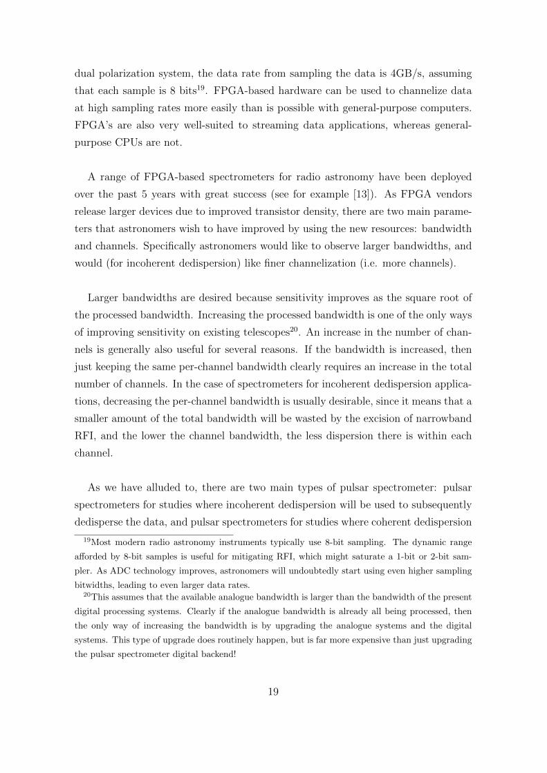
Figures 2.6 and 2.7 show the canonical data flow and functionality for spectrom-
eters for incoherent and coherent dedispersion applications respectively. The former
design produces a power spectrum (using a polyphase filterbank) that is then ac-
cumulated (integrated) before it is outputted. The output in modern instruments
is typically via Ethernet. The purpose of the accumulation stage is to reduce the
data rate to the point where all the data for an observation can be stored to hard
drives. The accumulator functions by summing the power spectra – it produces an
average21 power spectrum over the time that it sums over. There is a tradeoff in the
choice of accumulation length (i.e. how many spectra are summed in a single accu-
mulation/integration): the longer the accumulation length, the slower the data rate
becomes, but the worse the time-resolution of the instrument becomes. Typically
spectrometers for incoherent dedispersion applications have between 128 and 4096
channels, and time resolution of between several microseconds and several millisec-
onds. Bandwidths range from several tens of MHz through to 1GHz.
The spectrometer for coherent dedispersion applications is conceptually simpler –
it channelizes the input data (into chunks that typically have bandwidths between
1MHz and 50MHz) and then sends the raw polyphase filterbank output to a cluster,
via a switch. Because the data rate is too high for one computer to process, the output
is statically load balanced: the channels are divided amongst several machines. For
example, in a 32 channel system, there might be 8 processing computers, and so the
spectrometer will send 4 adjacent frequency channels to each processing computer
in turn. Because power spectra are not formed, it is not possible to accumulate the
data22. The compute cluster performs coherent dedispersion on the output channels
from the spectrometer in real time, because the data rate is typically too high to store
all the data.
For the purposes of testing a new pulsar observing system it is usually easiest to
attempt observations of bright (high flux) pulsars. Once the basic functionality of the
system has been verified (via the production of a correct pulse profile) it is then often
helpful to attempt an observation of a fast (small period) pulsar. Table 2.1 provides
21The accumulator does not divide its output by the number of spectra it added together.22The reason that the PFB output can’t be summed is essentially that pulsar signals look like
noise in the voltage domain, so an accumulation of the voltages would tend towards zero.
20
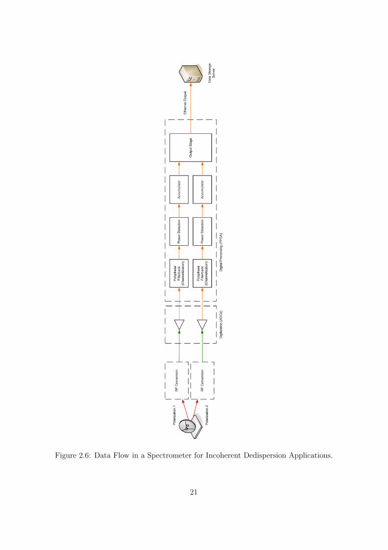
Figure 2.6: Data Flow in a Spectrometer for Incoherent Dedispersion Applications.
21
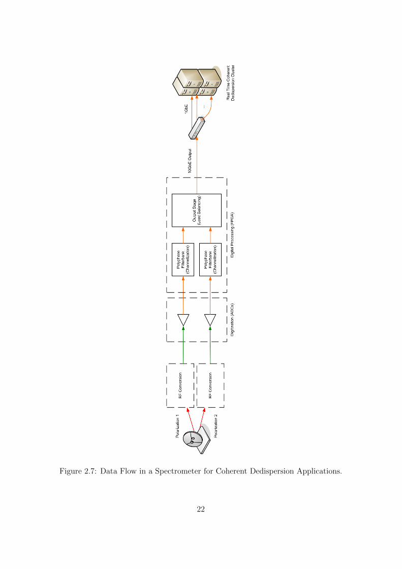
Figure 2.7: Data Flow in a Spectrometer for Coherent Dedispersion Applications.
22

a list of bright and fast pulsars that are useful test sources for Northern hemisphere
telescopes.
Table 2.1: From [9]. Pulsars Useful for Instrument Tests.
Name Period (s) Flux Density at 1.4GHz (mJy)
Fastest of the Very Bright
B0355+54 0.1563824177774 23
B1929+10 0.226517634984 41
B0950+08 0.2530651649482 84
B2020+28 0.3434021577859 38
B1933+16 0.3587384107696 42
B0329+54 0.7145196822210 203
Brightest of the Very Fast
B1937+21 0.0015578064724 16
B0531+21 0.03308471603 14
B1855+09 0.0053621004540 4
J1713+0747 0.0045701365242 3
J1012+5307 0.0052557490141 2.8
J1022+1001 0.0164529296832 2.3
2.5 CASPER
The Center for Astronomy Signal Processing and Electronics Research at the Uni-
versity of California, Berkeley, has developed a set of hardware and software tools
for building radio astronomy digital instrumentation. We have made extensive use of
their technology to develop the projects described in this thesis. In this section we
provide a brief overview of the CASPER technologies.
2.5.1 The CASPER Approach
CASPER was created as a result of the realization that digital signal processing
hardware technology, and especially FPGAs, have reached a point where it is pos-
sible to build almost all the digital instrumentation required in a radio telescope
23

from a common hardware platform. However, current practice is for observatories to
custom-build new hardware whenever they need a new instrument. This is not only
extremely wasteful of engineering effort, but also results in lengthened development
times for instruments.
CASPER therefore advocates an approach to building instrumentation that is
focused on reusability. In most cases the benefits that one obtains from custom-
designing a hardware processing board for a particular application are far outweighed
by the disadvantages in the additional cost and time that such development takes.
CASPER has developed a set of reusable, generic hardware modules that can be
used to develop a wide range of instruments, including spectrometers, correlators and
beamformers.
Another thrust of CASPER’s efforts is to encourage the use of industry stan-
dard communications protocols. Radio astronomy observatories have a history of
developing custom protocols for their instruments, which makes it very difficult for
instruments from different observatories to inter-operate, or for observatories to share
instruments with each other. CASPER advocates the use of industry-standard Eth-
ernet, XAUI [16] and 10Gb Ethernet [17] for instrument control, streaming data and
packetized data respectively.
2.5.2 CASPER Hardware
CASPER’s hardware offerings are described in detail in [13]. There are two current
processing boards, one digitization board, and one future processing board.
The IBOB (“Internet Break-Out Board”) is a processing board that has the abil-
ity to connect to two digitization boards, and has two 10GbE (CX4) ports and one
100MbE port. A basic block diagram for the IBOB is shown in Figure 2.8. The
IBOB’s centrepiece is a Xilinx Virtex 2 Pro VP50 FPGA, which includes two embed-
ded PowerPC cores (of which only one is used). For small instruments, such as the
pulsar spectrometers described in this thesis, this board can be used as a standalone
device. However, it can also be used as the first stage in larger instruments such as
correlators and beamformers, where a set of IBOBs is typically used for digitization
24
and channelization of all the antennas.
Figure 2.8: IBOB Block Diagram.
The iADC is a board that connects to the IBOB via a ZDOK connector. Each
iADC board includes two ADCs in a single IC package. The ADCs can be operated
individually, at 1GSa/sec each, or can be used in an interleaved mode that effectively
gives a sampling rate of 2GSa/sec.
CASPER’s large processing platform is the BEE2 [11]. This is a hardware plat-
form that includes five Xilinx Virtex 2 Pro VP70 FPGAs, which again each have two
embedded PowerPC cores. One FPGA, the “Control FPGA”, runs a modified version
of Linux, BORPH [15]. Each FPGA has at least two 10GbE ports available, and four
DDR2 DIMM sockets. This, combined with high-speed IO links between the FPGAs
on the board, makes the BEE2 an ideal platform for applications that require large
memory bandwidth or IO bandwidth.
ROACH (“Reconfigurable Open Architecture Computing Hardware”) is CASPER’s
next-generation processing board, built in collaboration with the Karoo Array Tele-
scope and NRAO Socorro. ROACH is intended as a replacement for IBOB and BEE2
boards in 2009. It features a single Xilinx Virtex 5 FPGA (either SX95, LX110T or
LX155T), four 10GbE ports, an external PowerPC for control and monitoring, 72Mbit
QDR SRAM and two DDR2 DIMM slots. It includes the same ZDOK connectors as
the IBOB, so that it can also be used with up to two iADC boards.
25

2.5.3 CASPER Toolflow and Libraries
Development for the IBOB, BEE2 and ROACH boards is supported using a toolflow
based on MATLAB’s Simulink graphical modeling tool, and Xilinx’s System Gener-
ator product, which allows for development of FPGA designs from within Simulink.
Xilinx’s EDK and ISE tools are used to build designs with PowerPC support.
The Simulink toolflow for the BEE2 was pioneered by Chen Chang, and is de-
scribed in his Ph.D. thesis [14]. Custom libraries for Simulink allow the hardware on
the BEE2, and other boards, to be accessed in Simulink designs. For example, there
are abstractions for the DRAM and 10GbE interfaces that are available on the BEE2.
The Simulink toolflow also provides the concept of “shared registers” and “shared
BRAMs”. These resources are physically implemented in the FPGA (just as regular
registers and BRAMs are), but are also connected to a bus that allows their values
to be accessed and manipulated from the embedded23 PowerPC. There is software
support to access these shared resources; the IBOB FPGA’s PowerPC runs a tel-
net server that exposes the resources, and the BEE2 control FPGA runs a modified
version of Linux, BORPH [15], that provides a filesystem abstraction for the resources.
In addition to hardware support in Simulink, there also exists a CASPER DSP
library that has been built specifically to provide the necessary DSP functions that
one needs to build radio astronomy instruments using the IBOB, BEE2 and ROACH
boards. The CASPER DSP library includes the following core components:
1. Streaming Parallel FFT
2. Polyphase Filterbank FIR Filter
3. Digital Downconverter
4. Arbitrary Reorder, and Transpose
23The ROACH board does not use an FPGA with an embedded PowerPC, but it supports shared
resources by exposing a bus that is connected to an external PowerPC. This PowerPC will also run
BORPH.
26
The DSP library also includes a set of useful “helper” blocks, such as counters that
freeze instead of wrap, blocks to detect positive and negative edges, and so on.
The streaming parallel FFT block is a streaming implementation of the FFT al-
gorithm that allows the designer to input 2k values per clock cycle, for arbitrary k.
This is crucial for applications where the ADC sampling frequency is higher than the
FPGA clock frequency, and a downconverter is not used. Typically the iADC will
be clocked at four times the rate of the FPGA on an IBOB, and hence each ADC
will present four samples every FPGA clock cycle. Therefore in order to compute a
spectrum, for example, it is necessary to have an FFT implementation that accepts
four values per clock cycle.
The Polyphase Filterbank FIR Filter is used in conjunction with the FFT to pro-
duce a polyphase filterbank (PFB). An ordinary FFT exhibits the phenomenon of
spectral leakage, whereby the value in one spectral channel “leaks” into adjacent
channels. This occurs because the input to the FFT is sampled, not continuous data.
The polyphase filterbank significantly reduces this spectral leakage by first convolving
the input data with a windowing function.
The Digital Downconverter is used to digitally extract a band of interest from the
sampled bandwidth. It is implemented in the standard way – using a lookup for the
sine and cosine functions, a “mixer” implemented using hardware multipliers, and an
FIR filter and decimation stage.
The Reorder and Transpose blocks have a variety of uses. Reordering is necessary
inside the FFT, but is also a common operation in instruments where it is useful to
group frequency components together, for example. An example of where a transpose
is necessary is in instruments that have two stages of channelization – a first FFT
does a coarse channelization, and then a second FFT further channelizes each result-
ing channel. For large matrices, a DRAM-based version of the Transpose function is
provided.
27

Chapter 3
The Fly’s Eye: Instrumentation for
the Detection of Millisecond Radio
Pulses
In this chapter we present the design and implementation of the “Fly’s Eye” in-
strument for the Allen Telescope Array. This instrument was purpose-built for an
experiment also known as “Fly’s Eye” to search for bright radio pulses of millisecond
duration. We designed and built a system containing 44 independent spectrometers
using 11 IBOBs. Each spectrometer processes a bandwidth of 210MHz, and produces
a 128-channel power spectrum at a rate of 1600Hz (i.e. 1600 spectra are outputted
by each spectrometer per second). Therefore each spectrum represents time domain
data of length 1/1600Hz=0.000625s=0.625ms, and hence pulses as short as 0.625ms
can be resolved1.
3.1 Science Motivation
In 2007, Lorimer et. al. [18] announced their discovery of a bright single pulse with
duration less than 5ms, which they deduced to be of extragalactic origin. Specifi-
cally, the 30Jy burst was dispersed with DM = 375cm−3 pc, which based on current
models of free electron content in the universe, Lorimer et. al. argue the source of
the burst to be up to 1Gpc distant. This, combined with the direction from which
the burst came, and other burst characteristics, indicate strongly that the burst is of
1Pulses of duration <0.625ms can also be detected provided that they are sufficiently bright, but
their length cannot be determined with a precision greater than the single spectrum length.
28

extragalactic origin. Figure 3.1 shows the pulse that Lorimer et. al. detected.
Figure 3.1: From [18]. The pulse discovered by Lorimer et. al. from data taken on
21 August 2001. The main graph shows the raw captured spectral data, in which the
dispersed pulse can clearly be seen. The inset image shows the same data after the
pulse has been dedispersed using DM = 375cm−3 pc.
The Lorimer et. al. pulse was discovered using the 64m Parkes Radio Telescope
with a 13-beam receiver. Each beam had a bandwidth of 288MHz, and the digital
backend produced 96-channel power spectra for each beam. Figure 3.2 shows the
beam pattern used. The detected pulse saturated the digitizer of one beam, and also
appeared in two adjacent beams, lending further credibility to the conclusion that
this was an astronomical signal, not an artifact in the instrumentation. A packed
beam pattern such as the one shown also helps to localize sources.
Lorimer et. al. found the pulse by dedispersing data from each beam with DMs
between 0 and 500 cm−3 pc and then searching the dedispersed data for individual
pulses with signal-to-noise ratios greater than 4. They processed 90 hours of data
from the source of the burst, and over 500 hours of data overall, and did not discover
any other pulses.
There is now significant interest in follow-up studies to try to detect more similar
pulses to further constrain the rate of their occurance, and to hopefully reveal more
29
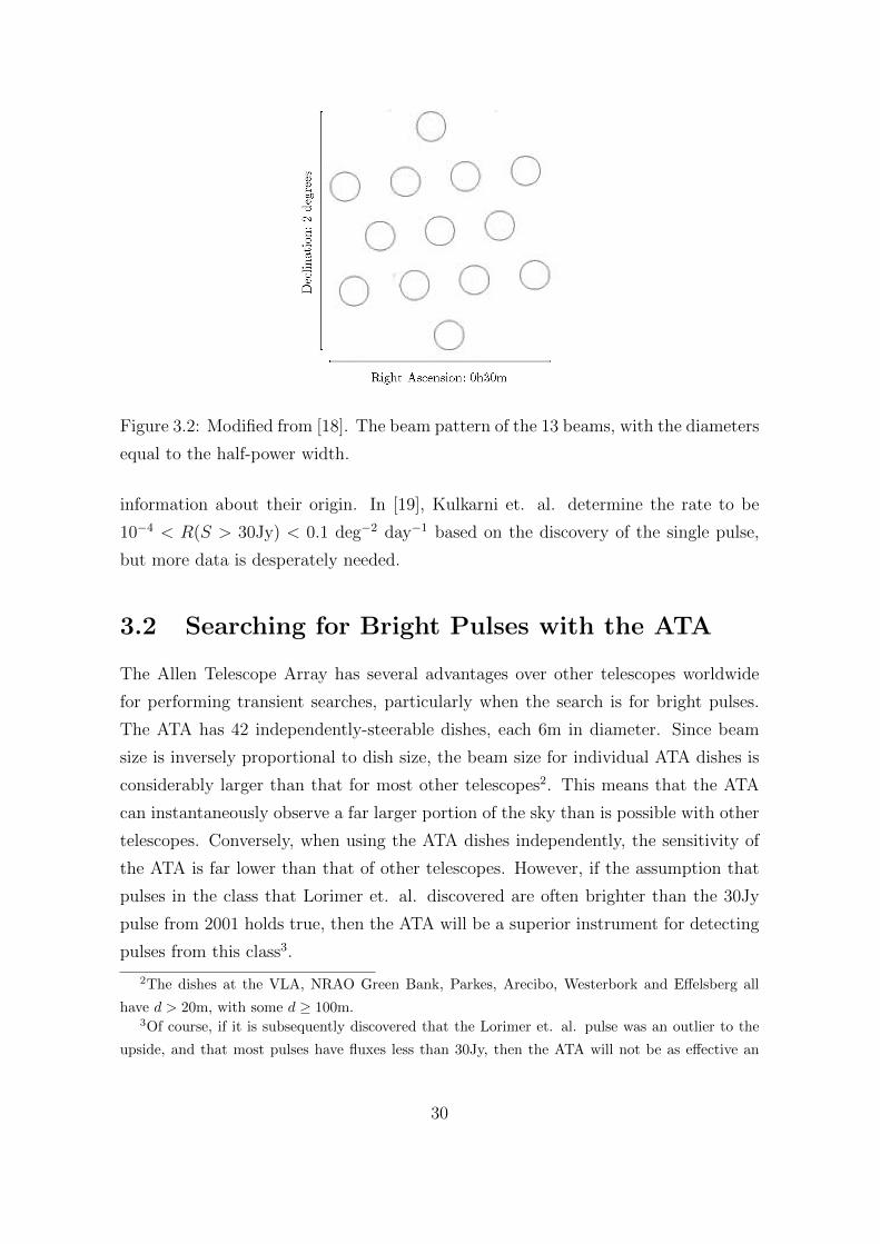
Figure 3.2: Modified from [18]. The beam pattern of the 13 beams, with the diameters
equal to the half-power width.
information about their origin. In [19], Kulkarni et. al. determine the rate to be
10−4 < R(S > 30Jy) < 0.1 deg−2 day−1 based on the discovery of the single pulse,
but more data is desperately needed.
3.2 Searching for Bright Pulses with the ATA
The Allen Telescope Array has several advantages over other telescopes worldwide
for performing transient searches, particularly when the search is for bright pulses.
The ATA has 42 independently-steerable dishes, each 6m in diameter. Since beam
size is inversely proportional to dish size, the beam size for individual ATA dishes is
considerably larger than that for most other telescopes2. This means that the ATA
can instantaneously observe a far larger portion of the sky than is possible with other
telescopes. Conversely, when using the ATA dishes independently, the sensitivity of
the ATA is far lower than that of other telescopes. However, if the assumption that
pulses in the class that Lorimer et. al. discovered are often brighter than the 30Jy
pulse from 2001 holds true, then the ATA will be a superior instrument for detecting
pulses from this class3.
2The dishes at the VLA, NRAO Green Bank, Parkes, Arecibo, Westerbork and Effelsberg all
have d > 20m, with some d ≥ 100m.3Of course, if it is subsequently discovered that the Lorimer et. al. pulse was an outlier to the
upside, and that most pulses have fluxes less than 30Jy, then the ATA will not be as effective an
30
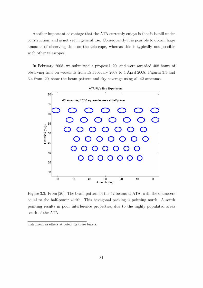
Another important advantage that the ATA currently enjoys is that it is still under
construction, and is not yet in general use. Consequently it is possible to obtain large
amounts of observing time on the telescope, whereas this is typically not possible
with other telescopes.
In February 2008, we submitted a proposal [20] and were awarded 408 hours of
observing time on weekends from 15 February 2008 to 4 April 2008. Figures 3.3 and
3.4 from [20] show the beam pattern and sky coverage using all 42 antennas.
Figure 3.3: From [20]. The beam pattern of the 42 beams at ATA, with the diameters
equal to the half-power width. This hexagonal packing is pointing north. A south
pointing results in poor interference properties, due to the highly populated areas
south of the ATA.
instrument as others at detecting these bursts.
31

Figure 3.4: From [20]. The sky coverage of the ATA for an observing period of 24
hours. Both the coverages for southern and northern pointings (corresponding to the
respective contiguous regions) are shown.
32

3.3 System Architecture
The overall architecture of the Fly’s Eye system is shown in Figure 3.5. Each IBOB
can digitize four analogue signals, and 11 IBOBs are provided so that 44 signals can
be processed. The ATA has 42 antennas, each with two polarization outputs. A
selection4 of 44 of the available 84 signals is made, and these are connected to the
44 iADC inputs. The IBOBs are connected to a control computer and a storage
computer via a standard Ethernet switch.
Figure 3.5: Fly’s Eye System Architecture. A selection of 44 analogue signals from
42 dual polarization antennas are connected to 44 independent spectrometers imple-
mented in 11 IBOBs.
Figure 3.7 shows the signal path at the ATA for the Fly’s Eye experiment. The
analogue frontend produces an IF band from 529MHz - 729MHz. The sky frequency is
fully controllable due to the presence of the controllable oscillator LO1 in the analogue
frontend architecture. We typically used a sky frequency of 1430MHz (i.e. observing
the band 1330MHz – 1530MHz). The IBOB ADCs are clocked at 838.8608MHz, so
4The selection is made with consideration for the goal of maximising field-of-view – in practice
we selected at least one polarization signal from every functioning antenna.
33
Figure 3.6: Fly’s Eye Rack at the ATA. Two 6U CompactPCI crates (top and bottom)
house the 11 IBOBs. The switch, data recorder computer and storage server are all
visible.
34

Figure 3.7: Signal path for the Fly’s Eye Experiment at the ATA.
35

the IF signal is in the second Nyquist zone. A digital downconverter (DDC) is used
to extract a 209.7154MHz band from 524.288MHz – 734.0032MHz.
3.4 A 210MHz Quad Spectrometer
The quad spectrometer design in each IBOB was based on the “Pocket Correlator”
(“PoCo”) design by Aaron Parsons [21]. The PoCo uses a 1024-channel PFB, whereas
the quad spectrometer design required only a 128-channel PFB. This 4-input FX cor-
relator produces power spectra for each input in addition to cross-terms created by
multiplying the spectrum from each input with that from every other input.
For the Fly’s Eye transient detection application, we are only interested in power
spectra, not the cross-terms that are calculated by a correlator. We wanted to obtain
the maximum dump rate possible with the 100MbE port on the IBOB, which, due
to processor bus constraints, is limited to a data rate of 7Mbps. Therefore it was
important to eliminate the cross-terms from the output, since their presence would
not only be wasteful, but would also greatly reduce the rate at which we could dump
power spectra, and hence would increase our integration time. This in turn would de-
grade our instrument’s sensitivity to short bursts. Hence we removed the cross-term
calculations from the PoCo design.
Two further important modifications were made to the PoCo design. To save re-
sources the PoCo resizes the output data width of the FFT from 18 bits to 4 bits. In
our design this is unnecessary, and we opted to maintain the full precision from the
FFT5. The output buffers in the PoCo were also significantly modified to provide the
option of a debug output of all 64 bits from the accumulators, and to maximize the
output data rate.
Figure 3.8 shows the final design of the modified PoCo design for the Fly’s Eye
experiment. It is effectively a fast-readout quad spectrometer. Four ADCs attached
to an IBOB sample four independent analogue signals at 838.8608MSa/sec. Each
digitized data stream is processed in parallel in the FPGA. First each signal is passed
through a digital downcoverter, which selects the band 104.8576MHz – 314.5728MHz
5Since the quad spectrometer only uses a 128-point FFT, there was an ample amount of logic
resources available so the full precision could easily be maintained.
36

from the sampled band 0 – 419.4304MHz. However, since the Fly’s Eye setup operates
in the second Nyquist zone, the selected band is actually (838.8608-314.5728)MHz –
(838.8608-104.8576)MHz, which is 524.288MHz – 734.0032MHz. This includes all of
the available signal that is provided from 529MHz – 729MHz (see the signal flow in
Figure 3.7). Next, the PFB FIR and FFT channelize each input into 128 bins. The
FFT output is passed to an “equalizer”, which allows the user to scale each frequency
bin by a specific constant. In practice we used this feature purely as a scale with no
frequency dependence, and instead performed equalization of the band in postpro-
cessing in software. The power spectrum is then computed (by summing the squares
of the real and imaginary parts of each FFT coefficient) and accumulated. Finally,
the accumulated spectra are written into the output stage BRAM buffers. A counter
is incremented when an accumulation is ready, and this signal is used by software
running on the PowerPC to determine when to start sending the next set of spectra.
Figure 3.9 shows this output stage in detail. The 64 bits produced by each accumu-
lator are separated into eight sets of 8 bits. The corresponding sets of 8 bits from all
four accumulators are concatenated to produce a 32-bit value that contains the same
order 8 bits from all four inputs.
During normal operation, only one set of 8 bits is outputted, but this setup al-
lows for a debug mode whereby all eight buffers are outputted, and hence all 64 bits
from each of the four inputs are made available. This is particularly useful when
the operator is deciding which 8 bits he or she should select to output, and what
scale coefficients are necessary. Figure 3.10 shows the interface between the FPGA’s
embedded PowerPC, the spectrometer design, and the external Ethernet interface.
The PowerPC software includes a module, the “UDP Output Controller”, that is re-
sponsible for detecting when a new accumulation is ready and sending it out over the
IBOB’s 100MbE interface as a UDP packet. If the bit selection parameter is specified
to request that all 64 bits be outputted, then this information will be used by the
UDP Output Controller, and it will concatenate the bits from the FPGA buffers to
recreate the original 64 bit accumulator outputs.
37
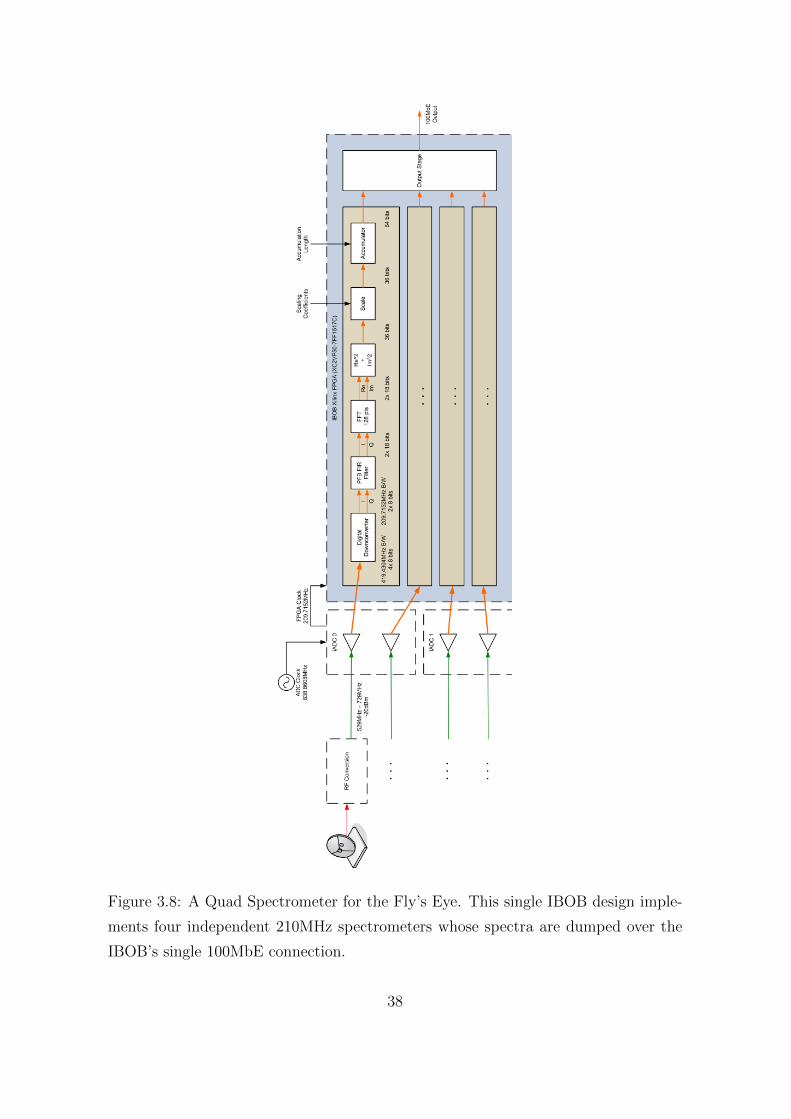
Figure 3.8: A Quad Spectrometer for the Fly’s Eye. This single IBOB design imple-
ments four independent 210MHz spectrometers whose spectra are dumped over the
IBOB’s single 100MbE connection.
38

Figure 3.9: The Output Stage of the Fly’s Eye Quad Spectrometer. All 64-bits from
each input’s accumulator are buffered, and code on the PowerPC determines which
set of 8 bits should be dumped.
39

Figure 3.10: PowerPC-FPGA Interface of the Fly’s Eye Quad Spectrometer. An
embedded PowerPC hosts a TCP Telnet server that processes user requests, includ-
ing the setting of parameters. A UDP output controller runs concurrently, and is
responsible for appropriately creating output data packets.
3.5 Observing Software
The Fly’s Eye system was set up for automatic operation, although at the start of
an observing session the operator needs to manually perform some setup and control
of the telescope array. We wrote a set of scripts to reset and sequentially configure
the IBOBs (with parameters such as accumulation length6, scaling coefficients and
bit selection). We wrote a script to set up the telescopes appropriately (it sets the
correct pointings and oscillator frequencies). Most importantly, we automated the
data recording and monitoring process: we created a script that runs on the control
computer that will manage an observation for a given period of time (typically 60
hours).
Figure 3.11 shows the overall architecture of the control and monitoring infras-
tructure for Fly’s Eye. A VNC session to the Fly’s Eye control computer is used to
run the IBOB configuration and observation scripts. Due to the fact that programs
running in a VNC session are by default not killed when the client-server connection
fails, we typically used the VNC session for all interactive user control, including
with the ATA control computer. The web server shown in this figure is used to host
6The accumulation length is determined by the “sync” pulse period parameter.
40

periodically-updated diagnostics from the Fly’s Eye control computer. The motiva-
tion for this is that during a long automated observation it is useful to have hourly
reports that the system is functioning correctly.
Figure 3.11: Fly’s Eye Control Architecture. The Fly’s Eye equipment is controlled
through a computer dedicated to the experiment; this machine is also responsible
for managing the data recording. The control of the general ATA infrastructure
(antennas and oscillators) is done through a separate, general-use control computer.
A remote web server is used to host diagnostic information.
Figure 3.12 shows the control flow in the scripts that run on the control computer
and web server during an observation. The control computer loops in a one hour cycle:
it does a 1-minute test observation, and follows it with a 58-minute observation. The
web server generates spectral plots from the test observation (44 independent plots)
so that the operator can periodically visit a website and have an easy visual check that
the system is functioning. After both the 1-minute and 58-minute observations a set
of diagnostics about the network connections and disk subsystems is also transferred
to the web server for inclusion in the diagnostic web pages.
41

Figure 3.12: Fly’s Eye Control Script Flow. The control computer alternates between
running a 1 minute test observation and a 58 minute live observation. The test obser-
vation data is transferred to the web server, where it is plotted and made available on
the web, along with other diagnostic information provided by the control computer.
42

3.6 Offline Processing to Detect Transients
The analysis required for the Fly’s Eye experiment is, in principle, fairly simple – we
wish to search over a wide range of dispersion measures to find large individual pulses.
Specifically our processing requires that all the data be dedispersed with dispersion
measures ranging from 50 cm−3 pc to 2000 cm−3 pc. At each dispersion measure the
data needs to be searched for ‘bright’ pulses. The practical definition ‘bright’ might
change depending on the scientist analysing the data, but essentially the task is to
search for pulses whose powers are greater than τσ+µ where τ is some user-specified
threshold (for example, τ = 10), σ is the standard deviation of the signal power, and
µ is the mean signal power.
The processing chain is in practice significantly more complicated than this de-
scription suggests. Processing is performed on compute clusters. Figure 3.13 shows
the major tasks in the processing chain. The head node’s purpose is to format and
divide the input data so that it can be assigned to worker nodes. In the worker node
flow, the data is equalized, then RFI rejection is performed, and finally a pulse search
is performed through the range of dispersion measures. The results are written to a
database where they can be subsequently queried. The key feature of the results is
a table that lists, in order of decreasing significance, the pulses that were found and
the dispersion measures they were located at.
3.6.1 Equalization
Equalization is the process of “equalizing” or “normalizing” the average signal power
in each frequency channel to some predetermined value. The power in channel i at
(discrete) time t is Pi(t) ∈ [0, 255], and we compute an average power per channel
Pi = 1T0
∑T0−1t=0 Pi(t) over some time period T0 (T0 is typically set to the length of a
data chunk, 10 minutes). A particular value Pi(t) is then equalized by dividing (using
floating-point arithmetic) by the average Pi. i.e. the equalized value P ′i (t) = Pi(t)/Pi.
The average power in each channel is thus unity, since 1T0
∑T0−1t=0 P ′i (t) = 1.
It is possible to equalize not only the frequency spectrum, but also the average
power across all channels. We would like to do this so that gain changes in the sys-
tem, which result in the average power increasing or decreasing over time (without
43

Figure 3.13: Fly’s Eye Cluster Processing Chain. The cluster head node is responsible
for providing formatted data chunks to the worker nodes on the cluster. The worker
nodes search a given chunk of data for bright pulses and write the results to a database
for later analysis.
44

regard for the source being pointed at), can be mitigated to a certain extent. Sharp
gain changes (those that occur in short periods of time) are undesirable, and our
equalization technique is only useful for smoothly-varying gain changes, such as those
caused by gradual change in temperature.
Average power equalization is performed on the frequency spectrum equalized val-
ues P ′i (t). We compute the average power over all frequency channels for a single
integration (time sample t). The power average is defined as P ′(t) = 1N
∑N−1i=0 P ′i (t).
N is the number of channels (for Fly’s Eye this is always 128). The motivation for
why it is possible to normalize the power is that we expect pulses to be dispersed
over many time samples, so this procedure should not remove extraterrestrial pulses.
With the average powers P ′(t), we can define the equalization of the powers P ′i (t).
The average power equalized values P ′′i (t) = P ′i (t)/P′(t). This procedure ensures that
the average power P ′′i (t) is normalized to unity.
3.6.2 RFI Rejection
We categorize types of RFI that we can expect as follows:
1. Constant (or near-constant) narrowband RFI
2. Short-timespan wideband RFI
3. Intermittent RFI (short-timespan and narrowband)
The first two types of RFI can be fairly easily detected using simple methods.
However, intermittent RFI (such as that which occurs when an aircraft with an ac-
tive radar flies through a telescope beam) is difficult to automatically excise.
Our strategy for mitigating constant narrowband RFI is simply to identify the
channels that are affected, and to exclude them from further processing. This channel
rejection is typically performed manually by looking at a set of spectra and identify-
ing obviously infected channels, which are then automatically excluded in subsequent
processing runs.
45

Short-timespan wideband RFI is detected automatically. If the RFI timespan is
significantly less than T0 (the averaging time for power equalization) then we can eas-
ily reject RFI by comparing, for each time t, the sum∑N−1
i=0 P ′′i (t) against some fixed
threshold. We expect that this sum will on average be unity, so a value significantly
higher than 1 is indicative of RFI. (It is important to set this threshold sufficiently
high that a genuine dispersed pulse will not trigger it – we found that for our data
a threshold of 10 appeared to eliminate all short-timespan wideband RFI without
accidentally removing bona fide astronomical data.)
Intermittent RFI is often quite difficult to automatically distinguish from gen-
uine astronomical pulses, and we followed a conservative approach to try to en-
sure that we do not accidentally excise dispersed pulses. Our statistic for inter-
mittent RFI is the variance of a single channel over a 10 minute data chunk, σ2i =(
1T0
∑T0−1t=0 (P ′′i (t))2
)−(
1T0
∑T0−1t=0 (P ′′i (t))
)2
. We empirically found a range for σ2i out-
side which it is likely that channel i contains time-varying RFI. Future reprocessing
will likely use a more robust method, such as that based on a kurtosis estimator [22].
Our final RFI mitigation technique is manual – in our results it is easy to see
high-σ hits that are a result of RFI: these hits appear as simultaneous detections at
many dispersion measures.
3.7 Test Results
We carried out a series of tests to verify the correctness of the instrument. The results
are described in this section.
3.7.1 Detection of the Hydrogen Spectral Line
The first test was to verify that the Fly’s Eye spectrometers produce correct spectra
on a long (multiple seconds) timescale. This is done by adding spectra together from
data collected over many seconds, and then viewing the resulting “integrated” spectra
to inspect them for relevant spectral features. In particular we expect to be able to
see the Hydrogen 21cm spectral line when the dishes are pointed at locations that
46

are known to contain much galactic gas. Figure 3.14 shows one-minute integrated
spectra for a single IBOB, in which a bump at ∼1420MHz is clearly visible. Similar
checks were carried out for all the IBOBs.
Figure 3.14: Fly’s Eye Spectra from a Single IBOB. All four spectra from a single
IBOB are shown, from a 1-minute test observation conducted on 18 February 2008.
The vertical axis is uncalibrated power in arbitrary units, and the horizontal axis is
frequency bin (0 - 127). The centre frequency is 1430MHz, and the ‘bump’ clearly
visible in all four spectra appearing several bins before bin 64 corresponds to the
expected frequency for the Hydrogen spectral line, 1420.40575MHz.
3.7.2 Detection of Pulses from PSR B0329+54
Once the long timescale Hydrogen spectral line test was successfully conducted, a set
of tests were carried out to verify that the spectrometers can be used to observe a
known pulsar. The first test was to observe a bright pulsar, PSR B0329+54, in the 44
spectra, incoherently summed to improve signal-to-noise. For this test, all the dishes
were pointed at PSR B0329+54. In this context incoherent summation means that
the power spectra from all 44 spectrometers were simply added together – this yields
a square-root improvement in sensitivity7. The incoherently summed spectra were
dedispersed using the known dispersion measure of PSR B0329+54. The data was
then folded at the known pulse period for the pulsar. Figure 3.15 shows the resulting
7In a beamformer the signals are typically added coherently – that is, the voltages are summed
after appropriate delays, not the powers. A beamformer yields a linear improvement in sensitivity,
but incoherent summation is a quick, crude technique for improving sensitivity.
47

pulse profile from a 15 minute observation.
After successfully detecting a pulsar in the incoherently summed data, the next test
was to detect a known pulsar in individual dishes. The same 15 minute set of data for
the summed test was used. However, instead of summing the spectra, each individual
stream of spectral data was dedispersed and folded. The resulting pulse profile plots
for all the spectrometers are shown in Figure 3.16. A pulse profile is clearly visible in
many spectrometers, but not in all of them. This turned out to be due to the fact that
the antennas at the ATA have varying signal-to-noise characteristics – the plots where
the pulse profile is clearly visible are connected to antennas that have a better SNR
measure than the antennas that yielded data in which the pulse profile cannot be seen.
3.7.3 Detection of Giant Pulses from the Crab Nebula
The detection of a pulsar by reconstructing its pulse profile is an excellent test to
verify that the short timescale behaviour of the spectrometers is sufficiently accurate
to detect dispersed pulses with very short duration. The final test to verify that
the Fly’s Eye instrument is capable of detecting the transients it was designed to
find is to use the instrument to detect an individual pulse from a pulsar. An indi-
vidual pulse from a pulsar is, to the instrument, indistinguishable from a transient
signal, so this test can provide great confidence that the instrument works as required.
A fundamental problem exists with attempting to detect a single pulse from PSR
B0329+54: despite the fact that this pulsar has the highest average flux of any known
pulsar, it is still too weak for individual pulses to be seen in individual ATA antennas,
or even in incoherently summed signals from all the dishes. Fortunately Nature pro-
vides a solution: the pulsar in the Crab nebula (the “Crab pulsar”) has a lower average
flux than PSR B0329+54, but its pulses are occasionally individually much brighter
than the individual pulses from PSR B0329+54. These so-called “giant pulses” can
be up to 1000 times brighter than the normal pulses [6]. Therefore a suitable test
of transient detection capability is to observe the Crab pulsar and attempt to detect
giant pulses from it.
Figure 3.17 shows a diagnostic plot generated from a one-hour Crab observation.
48

Figure 3.15: Pulse Profile of PSR B0329+54. Data taken from a 15-minute obser-
vation from 22 December 2007 were incoherently summed (44 analogue signals), and
folded using the known period of the pulsar PSR B0329+54, P0 = 0.7145s. The re-
peated, folded pulses are visible as dark lines in the time versus phase plot (bottom).
The pulse profile from folding several dedispersed pulses on top of each other is shown
above. Image courtesy Joeri van Leeuwen.
49

Figure 3.16: Pulse profiles calculated for all 44 independent spectrometers. Image
courtesy Joeri van Leeuwen.
50

The data is an incoherently summed set from the 35 best inputs (the 9 inputs in
which PSR B0329+54 could not be detected were discarded). The diagnostic plot
was generated after the raw data had been dedispersed using a range of dispersion
measures from 5 to 200. The Crab pulsar has dispersion measure ≈ 57 cm−3 pc, so
three giant pulses from the Crab pulsar can be easily identified in the lower plot. The
giant pulses appear only at the expected dispersion measure, whereas wideband RFI
appears across a wide range of dispersion measures.
Figure 3.17: Diagnostics on data taken from the Crab pulsar in a 60-minute obser-
vation conducted on 22 December 2007. The data was dedispersed using dispersion
measures ranging from 0 to 200 cm−3 pc. Top-left: single-pulse SNR histogram.
Top-centre: noise appears at all DMs, but bright pulses (SNR> 7) from the Crab
correctly appear at DM ≈ 57 cm−3 pc. Top-right: inset of Figure 3.18. Bottom:
pulse detections plotted on the DM versus time plane. Higher SNR detections appear
as larger circles. Three giant pulses from the Crab are clearly visible in this plot.
Image courtesy Joeri van Leeuwen, Griffin Foster and Andrew Siemion, from [20].
A frequency vs. time plot of the raw (summed) data at the time when the bright-
est giant pulses was detected is shown in Figure 3.18. The pulse is clearly visible in
the data, and a fit to the dispersion measure shows that the pulse is, nearly without
51

doubt, from the Crab (as opposed to RFI).
Figure 3.18: A giant pulse from the pulsar in the Crab nebula. This pulse was
detected in a 60-minute dataset taken on 22 December 2007. The dispersion of the
pulse, correctly corresponding to DM = 56.78 cm−3 pc, is clearly visible. Image
courtesy Griffin Foster and Andrew Siemion.
52

Chapter 4
Fast-readout 10GbE Spectrometers
for Incoherent Dedispersion
Applications
The spectrometers that we built for the Fly’s Eye experiment, whose design was dis-
cussed in the previous chapter, had a data output rate limitation of approximately
7Mbps. This limitation was imposed by the PowerPC 100MbE connection on the
IBOB; data is transferred from block RAMs in the FPGA via a bus to the embedded
PowerPC, and it is this bus that is the bottleneck. If the output data rate is less
than the input data rate (which for a dual polarization power/autocorrelation spec-
trometer is typically 2× 2×B × b bits per second, where B is the signal bandwidth
and b is the number of bits sampled), then the spectra have to be accumulated to
reduce the data rate, and this reduces the time resolution of the spectrometer. The
Fly’s Eye spectrometers had a time resolution of 625µs (calculated as the reciprocal
of number of spectra outputted per second). If one wishes to observe pulses that
have a duration less than 625µs, then it is advantageous for the spectrometer to have
a smaller (better) time resolution. Pulses from pulsars typically have a power that
is small compared to the noise power in the received signal, so the resulting reduc-
tion in power that occurs when the spectrometer time resolution is greater than the
pulse width can result in the pulsar being harder (or even impossible) to detect. It
is primarily for this reason that we want to build spectrometers that have high data
output rates.
In this chapter we describe our efforts to build several IBOB-based spectrome-
53

ters that all use a 10GbE connection to output data. This connection bypasses the
slow bus that restricts the data rate on the 100MbE connection. We built a dual
polarization, real sampling, 400MHz bandwidth power spectrometer for the Parkes
Radio Telescope. We modified this design for the Hartebeesthoek Radio Astron-
omy Observatory, which required a “Full Stokes” spectrometer. We also produced a
“Full Stokes” spectrometer for the Allen Telescope Array that could process 105MHz
bandwidth (the currently available bandwidth at ATA) and used a XAUI (digital)
connection from the ATA beamformer as its input, as opposed to digitizing analogue
inputs.
4.1 The Parkes and HartRAO Pulsar Spectrome-
ters
The Parkes and HartRAO spectrometer share a common architecture and set of fea-
tures. They were both designed to sample two real input signals at 800MSa/sec,
resulting in a 400MHz bandwidth being processed. Both designs use a single 10GbE
connection for data output. Both spectrometers use the 100MbE connection for con-
trol and testing. The primary differences between the spectrometers are the number
of channels (Parkes: 1024 channels, and HartRAO: 512 channels) and the products
computed (Parkes: powers only, and HartRAO: powers and cross-terms). The Parkes
spectrometer was designed for a new Parkes multibeam pulsar survey, which is an
experiment to search for new pulsars. Hence only powers are required. The Har-
tRAO spectrometer, on the other hand, will be used for polarimetry (polarization
studies), and this necessitates the output of the cross-correlations between the two
polarizations.
4.1.1 A 400MHz Fast-readout Dual Power Spectrometer for
Parkes
Figure 4.1 shows the design of the Parkes spectrometer. The two input polarizations
are digitized at 800MSa/sec. The FPGA is clocked off the ADC clock source, divided
by 4 on the iADC board; hence the FPGA is clocked at 200MHz. Every FPGA clock
cycle, four (8 bit) samples from each polarization are received by the FPGA. Two
streaming parallel polyphase filterbank FIR filters and FFTs are used to channelize
54

the data. A 2048 point “real” PFB is used; this implementation has optimizations
that take advantage of the fact that the imaginary part of the input is known to be
zero. Because the output of the FFT on real data is symmetric, the second half of
the spectrum is not outputted, hence only 1024 bins are produced.
The FFT output is scaled by a user-specified 18-bit coefficient. Each polarization
has a separate coefficient. A “power detector” then computes the power of this scaled
output, and the powers are summed in a vector accumulator. The length of the ac-
cumulator is a user-specified parameter. The accumulator has 32 bits of precision,
so the succeeding bit selection outputs 8 bits from 32; i.e. there are 4 possible bit
selection options – bits 0 – 7, bits 8 – 15, bits 16 – 23 and bits 24 – 31.
When the accumulator is outputting an accumulation, every clock cycle two sets
of 8 bits are produced by each polarization processing chain, and therefore 32 bits
are available to be outputted each clock cycle. The 10GbE interface has a data width
of 64 bits, so the concatenated data is buffered for one clock cycle every alternate
clock cycle; this technique is used to produce a set of 64 bits every second clock cycle
during output.
The output stage has a feature that is not shown in the high-level diagram Figure
4.1. In pulsar studies it is often necessary to know precisely the time of arrival of
pulses. It is also important to know if an accumulation is lost by the inherently un-
reliable UDP transport used between the IBOB and data recorder computer. Both
these requirements are satisfied by the inclusion of a time-stamping mechanism in the
design, which is detailed in Figure 4.2.
The 10GbE output stage includes a multiplexer that is used to insert the value
from a 64-bit counter at the start of each packet. This counter runs continuously
(that is to say, it is incremented every clock cycle), and is only reset to zero in the
following circumstance. The user asserts an ARM signal using the 100MbE control
link, and this state is stored in a boolean register. When the next 1PPS pulse arrives
at the FPGA, it is used to reset to the master counter if and only if the ARM state
register has value 1. This reset signal is used to reset the state register to zero. It is
also used to reset the sync pulse generator. The counter will not be reset again unless
the ARM signal is deasserted and then reasserted, due to the presence of a “positive
55

Figure 4.1: Parspec: a Dual Power Spectrometer for the Parkes Radio Telescope.
56
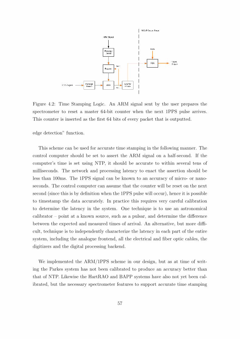
Figure 4.2: Time Stamping Logic. An ARM signal sent by the user prepares the
spectrometer to reset a master 64-bit counter when the next 1PPS pulse arrives.
This counter is inserted as the first 64 bits of every packet that is outputted.
edge detection” function.
This scheme can be used for accurate time stamping in the following manner. The
control computer should be set to assert the ARM signal on a half-second. If the
computer’s time is set using NTP, it should be accurate to within several tens of
milliseconds. The network and processing latency to enact the assertion should be
less than 100ms. The 1PPS signal can be known to an accuracy of micro- or nano-
seconds. The control computer can assume that the counter will be reset on the next
second (since this is by definition when the 1PPS pulse will occur), hence it is possible
to timestamp the data accurately. In practice this requires very careful calibration
to determine the latency in the system. One technique is to use an astronomical
calibrator – point at a known source, such as a pulsar, and determine the difference
between the expected and measured times of arrival. An alternative, but more diffi-
cult, technique is to independently characterize the latency in each part of the entire
system, including the analogue frontend, all the electrical and fiber optic cables, the
digitizers and the digital processing backend.
We implemented the ARM/1PPS scheme in our design, but as at time of writ-
ing the Parkes system has not been calibrated to produce an accuracy better than
that of NTP. Likewise the HartRAO and BAPP systems have also not yet been cal-
ibrated, but the necessary spectrometer features to support accurate time stamping
57

are available to the users.
4.1.2 A 400MHz Fast-readout Dual “Full Stokes” Spectrom-
eter for HartRAO
Figure 4.3 shows the design of the HartRAO spectrometer. This design is based on
that of the Parkes spectrometer. It differs primarily in that it computes both pow-
ers and cross-terms. This extra computation necessitated the reduction of the PFB
length from 1024 channels to 512 channels, and of the FFT precision from 18 bits
to 12 bits. The scaling from the Parkes design, which allows the two polarizations
to be independently scaled directly following the FFT, is retained. An additional
scaling is performed after the power and cross-term calculations, since the power and
cross-term values are expected to differ significantly. Because each set of FFT bins is
used to produce four values (the two powers, and two cross-terms), the vector accu-
mulator produces a total of eight 32 bit values per clock cycle while an accumulation
is being outputted. After bit selection, eight 8 bit values are available per clock cycle,
and hence the concatenated output can be connected directly to the 64-bit 10GbE
controller, without the need for the buffering scheme in the Parkes design.
4.1.3 Test Results
The Parkes power spectrometer design was tested both at the NRAO Green Bank
140ft telescope, and at the Parkes Radio Telescope. Figure 4.4 shows the pulse pro-
file for PSR B1937+21 obtained after a 30 minute observation at NRAO by Glen
Langston and co-workers. PSR B1937+21 is a fast millisecond pulsar, and has a pe-
riod of approximately 1.56ms. It is therefore a demanding test of the spectrometer’s
capabilities. The obtained pulse profile correctly shows the double peak characteristic
of this pulsar.
Figure 4.5 shows the pulse profile (and associated diagnostic plots) obtained from
an observation of PSR J1028-5820 conducted using the Parkes Radio Telescope. The
produced pulse profile shows excellent time resolution.
Figure 4.6 shows the pulse profile obtained from an observation of B0833-45 (Vela)
conducted using the HartRAO telescope. The observation was performed at a centre
frequency of 1668MHz over 20 seconds. The pulse profile produced is very closely
58

Figure 4.3: A Dual “Full Stokes” Spectrometer for the Hartebeesthoek Radio Astron-
omy Observatory.
59

Figure 4.4: Pulse profile of PSR B1937+21 obtained using the Parkes Spectrometer
with the NRAO Green Bank 140ft telescope. Image courtesy Glen Langston, Paul
Demorest and Scott Ransom (NRAO).
60
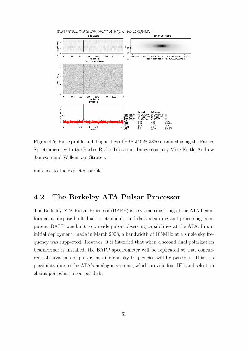
Figure 4.5: Pulse profile and diagnostics of PSR J1028-5820 obtained using the Parkes
Spectrometer with the Parkes Radio Telescope. Image courtesy Mike Keith, Andrew
Jameson and Willem van Straten.
matched to the expected profile.
4.2 The Berkeley ATA Pulsar Processor
The Berkeley ATA Pulsar Processor (BAPP) is a system consisting of the ATA beam-
former, a purpose-built dual spectrometer, and data recording and processing com-
puters. BAPP was built to provide pulsar observing capabilities at the ATA. In our
initial deployment, made in March 2008, a bandwidth of 105MHz at a single sky fre-
quency was supported. However, it is intended that when a second dual polarization
beamformer is installed, the BAPP spectrometer will be replicated so that concur-
rent observations of pulsars at different sky frequencies will be possible. This is a
possibility due to the ATA’s analogue systems, which provide four IF band selection
chains per polarization per dish.
61

Figure 4.6: Pulse profile of PSR B0833-45 (Vela) obtained using the HartRAO Spec-
trometer with the 26m HartRAO dish. Image courtesy Sarah Buchner (HartRAO).
4.2.1 Overall Architecture
Figure 4.7 shows the overall architecture for the Berkeley ATA Pulsar Processor sys-
tem, as it was deployed. Two single polarization 26-antenna beamformers send their
output to a “polarization aligner”, which aligns the two different polarization beams
and outputs the combined dual polarization beam over a XAUI connection. Recall
from Chapter 2 that a beamformer delays the signals from the 26 antenna inputs ap-
propriately so that an effective narrow beam on the sky is formed. The polarization
aligner is effectively a final stage in what can be considered a dual polarization beam-
former – it delays the one polarization beam relative to the other polarization beam
so that they are aligned in time. This dual polarization signal is sent to the BAPP
spectrometer, which is the BAPP subsystem that we are primarily concerned with in
this thesis. (For more details on the ATA beamformer systems, see reference [12].)
The data output from the spectrometer is over a 10GbE connection; this is converted
to a 1GbE connection by an HP 10GbE/1GbE switch (an HP ProCurve 2900-24G),
which is connected to a data recorder computer. The motivation for this wasteful
use of a 10GbE connection to carry a data bandwidth of less than 1Gbps is that a
data rate of greater than 7Mbps is required to get suitable time resolution, but the
IBOB has no Ethernet interfaces other than its 100MbE port and its 10GbE ports.
Since the 100MbE port is not capable of outputting data faster than 7Mbps, a 10GbE
62
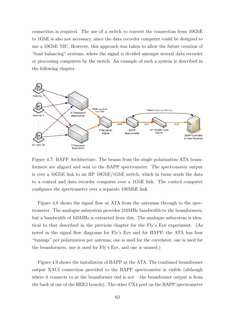
connection is required. The use of a switch to convert the connection from 10GbE
to 1GbE is also not necessary, since the data recorder computer could be designed to
use a 10GbE NIC. However, this approach was taken to allow the future creation of
“load balancing” systems, where the signal is divided amongst several data recorder
or processing computers by the switch. An example of such a system is described in
the following chapter.
Figure 4.7: BAPP Architecture. The beams from the single polarization ATA beam-
formers are aligned and sent to the BAPP spectrometer. The spectrometer output
is over a 10GbE link to an HP 10GbE/1GbE switch, which in turns sends the data
to a control and data recorder computer over a 1GbE link. The control computer
configures the spectrometer over a separate 100MbE link.
Figure 4.8 shows the signal flow at ATA from the antennas through to the spec-
trometer. The analogue subsystem provides 210MHz bandwidth to the beamformers,
but a bandwidth of 105MHz is extracted from this. The analogue subsystem is iden-
tical to that described in the previous chapter for the Fly’s Eye experiment. (As
noted in the signal flow diagrams for Fly’s Eye and for BAPP, the ATA has four
“tunings” per polarization per antenna; one is used for the correlator, one is used for
the beamformers, one is used for Fly’s Eye, and one is unused.)
Figure 4.9 shows the installation of BAPP at the ATA. The combined beamformer
output XAUI connection provided to the BAPP spectrometer is visible (although
where it connects to at the beamformer end is not – the beamformer output is from
the back of one of the BEE2 boards). The other CX4 port on the BAPP spectrometer
63
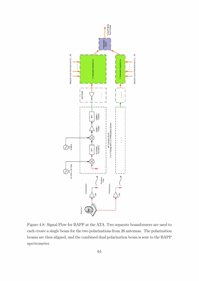
Figure 4.8: Signal Flow for BAPP at the ATA. Two separate beamformers are used to
each create a single beam for the two polarizations from 26 antennas. The polarization
beams are then aligned, and the combined dual polarization beam is sent to the BAPP
spectrometer.
64

IBOB is attached to the HP ProCurve 2900 10GbE/1GbE switch. The 100MbE con-
trol and test connection cable to the IBOB (purple) is also visible. This is connected
to the Data Recorder computer via the switch, although this is not visible, since the
switch is installed with the front panel facing backwards1.
Figure 4.9: BAPP Installation. The rack in which BAPP is installed at the Allen
Telescope Array is shown. The leftmost (partially) visible rack contains the RF
conversion subsystem. The middle rack contains the beamformer (with digitization
at the top, using IBOBs, and processing at the bottom, using BEE2s). The rightmost
rack contains the BAPP hardware, in addition to several other unrelated pieces of
equipment. (Figure compressed to meet arXiv file size requirements.)
4.2.2 A 105MHz Fast-readout Dual Spectrometer with Dig-
ital Beamformer Interface
The spectrometer design for BAPP is based on the Parkes and HartRAO designs.
Because the bandwidth requirement for BAPP was only 105MHz, versus 400MHz for
the Parkes and HartRAO spectrometers, it was possible to fit a Full Stokes 2048-
channel design onto the IBOB FPGA. Instead of processing four (real) parallel data
streams, the BAPP design runs at 105MHz and processes only one (complex) data
stream per polarization. As discussed, the input is a dual polarization beam that is
1This was done to reduce the length of the cable for the 10GbE connection from the IBOB to
the switch, since the 10GbE ports on the switch are at the back.
65

streamed over a XAUI connection from the ATA beamformer system. Figure 4.10
shows the design of the BAPP spectrometer. An implementation detail that appears
in this diagram is that an iADC board is still used, even though the input is digital –
it was necessary to use an iADC to clock the IBOB externally, with a clock frequency
identical to that of the beamformer. The CASPER DSP blocks are designed to
be continuously streaming, so the received XAUI data in the spectrometer had to
produce one sample of data every FPGA clock cycle, and the only way to ensure this
is to have the receiver be clocked at an identical2 rate to the sender.
4.2.3 Test Results
The BAPP system underwent a set of tests to verify its functionality. The first
test was an elementary one designed to verify that the data from the beamformer
was being received correctly: the beamformer was configured to output a tone at a
specific frequency, and the BAPP power spectra outputs were plotted to check that
peaks at the appropriate locations in the spectra were visible. The tone was then
moved and scaled, and the BAPP output was again inspected to make sure that the
peaks had moved and been scaled as expected. With the basic functionality of the
system verified, we proceeded with two astronomical tests.
Detection of the Hydrogen Spectral Line
The first astronomical test was designed as the simplest possible end-to-end verifica-
tion of the BAPP system. The beamformer was calibrated, and then the array was
pointed at a source with a significant Hydrogen content. The power spectra outputs
were integrated for a one-minute observation, and we verified the presence of the
Hydrogen spectral line in the spectra.
Detection of Pulses from PSR B0329+54
The second astronomical test was to observe a pulsar, and form a pulse profile from
that observation. We observed PSR B0329+54, which is sufficiently bright that indi-
vidual pulses from the pulsar can be detected in the beamformed signal. Figure 4.11
shows a set of 100 individual pulses from PSR B0329+54, and the resulting integrated
2As is the standard practice at observatories, the clock sources at the ATA are synchronized via
a distributed 10MHz signal, so all the clock sources are in phase. Therefore the sending BEE2 and
the receiving IBOB in the BAPP system are clocked using sources that are in phase.
66

Figure 4.10: The Berkeley ATA Pulsar Processor Spectrometer: a 105MHz Fast-
readout Dual Spectrometer with Digital Beamformer Interface
67

pulse profile. These pulses are shown after the signal has been dedispersed (with the
appropriate, known, dispersion measure) on the BAPP processing computer.
68

Figure 4.11: Detection of Individual Pulses from PSR B0329+54. Image courtesy
Joeri van Leeuwen. (Figure compressed to meet arXiv file size requirements.)
69

Chapter 5
A Load Balanced Spectrometer for
Coherent Dedispersion
Applications
Coherent dedispersion, as opposed to incoherent dedispersion, is used in experiments
where it is important to reverse completely the dispersive effect of the interstellar
medium [6]. Coherent dedispersion is more computationally intensive than incoher-
ent dedispersion, so typically a cluster of computers will be used to dedisperse a
bandwidth B > 50MHz. The coherent dedispersion algorithm acts on “raw” complex
voltages, not powers, so data cannot be accumulated (as is the case with data pro-
duced for incoherent dedispersion applications). Therefore the output data rate of
a spectrometer for coherent dedispersion applications is directly related to the input
bandwidth and the output sample bitwidth.
5.1 Overall Architecture
Figure 5.1 shows a potential system architecture for an experimental setup to conduct
a coherent dedispersed-based pulsar study. Two polarization signals from an antenna
are provided as real (i.e. not downconverted) voltages with bandwidth 400MHz. A
spectrometer divides the signals into 32 channels each; each polarization’s channels
are outputted over a separate 10GbE connection. Since a single workstation-class
computer is not able to perform coherent dedispersion on a 400MHz bandwidth sig-
nal in real time, the workload needs to be spread over several computers. The 10GbE
70

connections are therefore terminated at a switch, which is connected to 8 computers
using 1GbE connections, and each computer processes 1/8th of the bandwidth.
Figure 5.1: System Architecture for a Coherent Dedispersion Pulsar Study.
Recent investigations into using graphics processing units (GPUs) to accelerate
coherent dedispersion calculations [24, 25] suggest that it will be possible to dedis-
perse coherently a dual polarization signal with a bandwidth of 50MHz using a sin-
gle nVidia GT280 GPU. Four computers each equipped with two such GPUs could
then coherently dedisperse a 400MHz bandwidth. In this case each computer needs
to receive a 100MHz bandwidth; an 8-bit sample bitwidth implies a data rate of
2 polarizations× 200MSa/sec× 1byte/sample = 400Mbytes/sec = 3.2Gb/sec. Either
four 1GbE connections could be supplied to each computer, or a single 10GbE connec-
tion from a 10GbE switch could be used. Due to the use of standard Ethernet output
in the design presented in this chapter, and the availability of both 10GbE/1GbE
and many-port 10GbE switches, both options are possible without any modification
to the spectrometer design.
71

5.2 A Static Load Balancing 400MHz Dual Spec-
trometer
Figure 5.2 shows the overall design of an IBOB-based dual polarization spectrometer
that outputs complex Fourier coefficients (i.e. channelized complex voltages) over two
10GbE ports (one for each polarization). The spectrometer was built for the Nancay
Radio Telescope, which supplies an IF at baseband. Hence the spectrometer accepts
real baseband signals from 0 – 400MHz as input.
Conceptually the design is fairly simple: an input signal is digitized and channel-
ized using a 64-point polyphase filterbank to produce 32 channels. The PFB uses
18 bits of precision, and this is requantized to 8 bits. A scaling function is provided
so that the user can shift the bits to select the most significant toggling ones. This
stream of 8-bit numbers is sent to the 10GbE output stage. The output stage groups
data values by channel (using a reorder block) before transmitting them. The output
is statically load-balanced – the user can set which frequency channels are sent to
which IP address.
The channelization part of this instrument’s design is very similar to that of the
designs described in the previous chapter. The output stages1, however, have sig-
nificant differences. Figure 5.3 shows a high-level view of the output stage in our
prototype design. Every clock cycle the output stage receives four 8-bit values from
the channelization stage: the real and imaginary parts of two consecutive channels.
As is the case with the output stages in our other instruments, we need to buffer
every second set of data because the data bus width of the 10GbE core is 64 bits.
One new feature of this output stage is its support of static load balancing by
allowing the user to specify lists of destination IP addresses and ports. These lists
are each stored in a single shared BRAM. Previously two shared registers, allowing
the user to specify only one IP address and one port, were provided. A fairly simple
design involving a wrapping counter is needed in an “Address Generator” unit to
enable the design to change destination details at appropriate intervals.
1The design includes two identical output stages, one for each polarization.
72
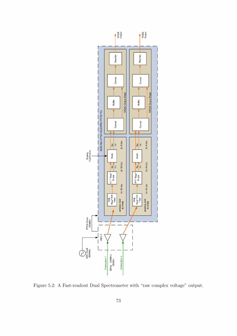
Figure 5.2: A Fast-readout Dual Spectrometer with “raw complex voltage” output.
73

Figure 5.3: The 10GbE Output Stage.
74

A simple approach to implementing static load balancing is to simply send out
packets containing four adjacent spectral bins. Every clock cycle the output stage
receives two new bin values, so every two clock cycles it has four bins (comprising 64
bits) that can be sent over 10GbE. This is a very simple scheme to implement, since it
simply requires that every second clock cycle the Address Generator should increment
to select a new address from the IP and port BRAMs. However, there is a practical
consideration that causes this approach to fail. We performed a set of network tests
on a typical compute server with a 1GbE NIC and found that even with relatively low
data rates (< 50MB/sec) the server would drop a high percentage of packets (> 50%)
if the packet payload size was sufficiently small (due to the high interrupt rate, which
the CPU was apparently unable to satisfactorally service). Packet sizes larger than
100 bytes were found to yield vastly improved packet loss statistics.
This finding about packet sizes suggests that a successful approach to static load
balancing of spectral data will require that each sent packet have a payload of at least
100 bytes. We chose the value 256 bytes, since this is sufficiently large that packet
loss becomes negligible, but not so large that it is not possible to fit the required
buffer into the FPGA design.
It is desirable to perform the load balancing in such a way that the compute servers
receive packets with adjacent spectral bins. It is not desirable to have the spectrom-
eter output different time samples containing all spectral bins to a single compute
server. Therefore the easiest means of increasing the packet payload size – simply in-
creasing the number of clock cycles that the output stage spends on each destination
before moving to the next destination in the list – is not acceptable. What needs to
happen instead is for the output stage to build large (256 byte) packets containing
many time samples of some small set of bins.
If we define the input to the output stage at any one clock cycle as ft(k) ∈ C and
ft(k+1) ∈ C (where t is a time index denoting the spectrum, and k ∈ 0, 2, . . . , 30 are
the channel/bin numbers), what we desire is to form eight packets Pi (i ∈ 0, 1, . . . , 7)whose contents consists of four adjacent spectral bins from 32 spectra. For example,
P0 = ft(0), ft(1), ft(2), ft(3), ft+1(0), . . . , ft+1(3), . . . , ft+31(0), . . . , ft+31(3). More
generally,
75
Pi = ft(4 · i), ft(4 · i+ 1), ft(4 · i+ 2), ft(4 · i+ 3), . . . , ft+31(4 · i), . . . , ft+31(4 · i+ 3)
The order that the output stage receives data in is:
ft(0), ft(1) , . . . , ft(30), ft(31) , ft+1(0), ft+1(1) , . . . , ft+1(30), ft+1(31) , . . .
Braces here denote values that arrive on the same clock cycle. It is now easy to see
that if we wish to create Pi starting with i = 0 and continuing through i = 7 before
returning to i = 0, a simple solution is to reorder the data received by the output
stage. The reorder definition is as follows:
0, 1, . . . , 1024 7−→ 0, 1, 2, 3, 32, 33, 34, 35, . . . , 992, 993, 994, 995, 4, 5, 6, 7, . . .
This reordering can easily be implemented using the CASPER “Reorder” block.
The only further modification required to support the creation of large packets is to
the Address Generator, which needs to only increment the address counter every 64
clock cycles.
The final part of the output stage before the 10GbE interface block is a “header
insertion” stage that, as the name suggests, inserts a header at the start of each
packet to be sent. This header is simply a 64-bit counter value that is used both for
timing purposes and for detecting packet losses.
5.3 Test Results
Time constraints relating to the acquisition of equipment at the Nancay Radio Tele-
scope resulted in us not being able to conduct field tests of our prototype2. However,
we conducted basic functional tests in the lab. Specifically we were able to divide the
spectrum between two computers through a 10GbE/1GbE switch. (The instrument
design allows for 8 different IP addresses (and port numbers) per polarization, so we
2Note added in proof: From 2 – 5 September 2008, a variant of the instrument described in this
chapter was deployed in Nancay. During this week we successfully observed, and produced pulse
profiles for, the pulsars PSR B1237+25 and PSR B1133+16.
76
used each IP address 8 times.) We conducted a “tone test” to verify that the spec-
trometer was working – this involves directly attaching a sine wave source to an ADC
input and verifying that a peak appears in the appropriate bin(s) in the resulting
power spectrum. On the receiving computer end we computed the power spectrum
by squaring the sums of the real and imaginary parts of the Fourier coefficients that
are transmitted by the instrument. Since the channelization portion of the design
has been well tested in several other instruments, we are confident that the prototype
will produce correct results in a production environment. Our tone tests verified the
functionality of the new portion of the design, the load-balancing output stage.
77

Chapter 6
Conclusions
In this thesis we have described the development of and results from several spec-
trometer instruments that were purpose-built for transient and pulsar studies. We
obtained satisfactory field results from our ATA Fly’s Eye, Berkeley ATA Pulsar
Processor, Parkes Spectrometer and HartRAO Spectrometer instruments. We also
presented work on the design of a prototype spectrometer system for coherent dedis-
persion applications, and an investigation into the design of an FPGA-based real-time
coherent dedispersion system.
Throughout we have used the CASPER hardware and tools, as we set out to do,
and we have verified the functionality and ease-of-use of many aspects of the hardware
and the DSP library.
6.1 Results Obtained
We developed four field-tested instruments: the Fly’s Eye, BAPP, the Parkes Spec-
trometer and the HartRAO Spectrometer. Each instrument was tested at at least one
operational radio telescope facility and verified to perform adequately for the tasks
for which they were design.
Specifically the ATA Fly’s Eye instrument was verified through observations of
PSR B0329+54 and the Crab pulsar, and through observations of giant pulses from
the Crab. These giant pulses were detected using the same search mode that is used
to find bright transient pulses, and hence verified the end-to-end capability of the
78
system to detect the class of signal the instrument was designed to find.
The Berkeley ATA Pulsar Processor spectrometer was successfully integrated with
the ATA beamformer. An observation of individual pulses from PSR B0329+54 using
24 dishes forming one beam verified the end-to-end functionality of the system. The
pulse profile obtained using BAPP showed excellent agreement with existing profile
data.
The Parkes spectrometer was tested and verified at both NRAO Green Bank and at
the Parkes Radio Telescope. An observation of the fast millisecond pulsar B1937+21
yielded a correct pulse profile and verified the spectrometer’s functionality for small-
period pulsars. An observation of PSR J1028-5820 with the Parkes Radio Telescope
verified the spectrometer’s functioning in the Parkes Radio Telescope setup (for which
it was designed), and showed excellent time resolution.
The HartRAO spectrometer was tested at HartRAO with observations of Vela and
several other pulsars. The Vela pulse profile was in excellent agreement with existing
profile data.
6.2 Future Work
The CASPER hardware successor to the BEE2 and IBOB, the ROACH board, is
to be released from beta testing in early 2009. We expect that it will be possible
to implement 700MHz dual polarization spectrometer designs on the ROACH board
without considerable effort. The ports of the Parkes and HartRAO spectrometers to
ROACH should be relatively easy, and will not only increase the available bandwidth,
but should allow for improved spectral resolution.
Both the ATA Fly’s Eye and BAPP instruments are bandwidth limited by the
supplied signal, so an upgrade to ROACH would not yield improvements to the
bandwidth. However, improved spectral resolution (and in the case of Fly’s Eye,
time resolution) should be fairly simple to achieve.
Once ROACH is available, it will be interesting to investigate its capabilities with
79

the development of a real-time coherent dedispersion system in mind. An implemen-
tation of the BEE2-based design presented in Appendix A would allow for such an
investigation – the remaining work would be to discover what values of N (num-
ber of channels) and M (FFT length) are achievable in practice. Real-time coherent
dedispersion is a significant computational challenge, and a successful implementation
using ROACH could have a significant impact on the pulsar observing community due
to potential improvements in price/performance by switching from cluster computing
to an FPGA processing approach.
80
Appendix A
Investigation into Building a
FPGA-Based Real-Time Coherent
Dedispersion System
Coherent dedispersion is used when the best possible time resolution is required.
The coherent dedispersion algorithm operates on “complex voltages” (i.e. complex
Fourier coefficients), and hence the data rate prior to dedispersion cannot be re-
duced by accumulation. Therefore observing large bandwidths will result in large
data rates to the coherent dedispersion system. Typically coherent dedispersion is
done in pseudo-real-time using compute clusters, because it is not feasible to store the
complex voltages for later processing. However, the processing demands for current
typical observable bandwidths (100MHz < B < 1GHz) are significant. In order to
dedisperse coherently a dual polarization 1GHz signal, approximately 15 modern dual
quad-core CPU compute servers are necessary [26]. Even next-generation GPUs are
not expected to provide a simple solution: approximately 20 nVidia GT280 GPUs
will be needed to coherently dedisperse 1GHz [25].
One potential alternative to using compute clusters is to use an FPGA-based sys-
tem. Coherent dedispersion is a relatively simple algorithm that involves two discrete
Fourier transforms (the forward and inverse transforms), and multiplication. The
data supplied to the procedure can be streaming, so FPGA implementations offer
much promise.
In this chapter we present a high-level investigation into the design of a real-time
81

coherent dedispersion system using FPGAs. We did not implement the ideas pre-
sented to the point of producing a prototype.
A.1 Coherent Dedispersion on Compute Clusters
Before we can discuss FPGA implementations of coherent dedispersion, we first need
to provide some detail on how this task is performed on conventional compute clusters.
Consider the case where the input bandwidth B is split into N channels using
a polyphase filterbank, and these N channels are sent to N compute servers (one
frequency channel per server). The data Si arriving at each server i can then be
considered as complex samples of a B/N bandwidth signal.
The coherent dedispersion of a discrete signal Si [t] (where t is discrete time) is
calculated as the convolution of Si [t] with a “chirp” function that is designed to re-
verse the dispersion in the signal. Convolution in the time domain is equivalent to
multiplication in the frequency domain – because the discrete Fourier transform (and
its inverse) can be efficiently calculated using the FFT algorithm, it is more efficient
to apply the dedispersion filter in the frequency domain. The filter’s definition [6] is:
H(f0 + f) = ei 2πD(f+f0)f
20
DMf2
Here f0 is the centre frequency, D is the dispersion constant and DM is the disper-
sion measure. The procedure then is to obtain the discrete Fourier transform, Si [f ],
of the signal Si [t], to multiply this with a discrete version of H(f0 + f), and to then
apply the inverse DFT to this result to produce a dedispersed time series of complex
samples.
There is an important practical consideration in this procedure that can greatly
affect the implementation of the algorithm: the length of the chirp function to be
used (i.e. how many values are in its domain). This length determines the number
of points required in the FFTs [25]; specifically there needs to be an overlap between
82

FFTs of at least the chirp length, so the FFT length needs to be the nearest power-
of-two that is at least twice as large as the chirp length.
The chirp length is dependent on the observing frequency f0, the bandwidth of
the channel B/N , and the dispersion measure, DM, to be applied. It can differ quite
significantly, as Table A.1 shows.
Table A.1: Table courtesy Ismael Cognard. Chirp Function and FFT Lengths Re-
quired for Coherent Dedispersion. f0 is the centre frequency, and B/N is the channel
bandwidth.
DM (pc cm−3) Chirp Length FFT Length
f0 = 1.4GHz, B/N = 16MHz
250 193586 512k
500 387172 1M
1000 774344 2M
f0 = 1.4GHz, B/N = 8MHz
250 48396 128k
500 96793 256k
1000 193586 512k
f0 = 1.4GHz, B/N = 4MHz
250 12099 32k
500 24198 64k
1000 48396 128k
In CPU and GPU implementations, the primary limitation that prevents the effi-
cient execution of arbitrarily large FFTs is memory. Since the dedispersion procedure
needs to be performed in real-time, a limit on the coherent dedispersion capabilities
of a particular cluster system is defined partially by the largest FFT the system can
perform and still meet the real-time requirement. We will see that a similar limitation
exists, albeit for a different reason, in FPGA-based systems.
83

A.2 Coherent Dedispersion on CASPER Recon-
figurable Computing Platforms
A real-time coherent dedispersion system implemented using FPGAs needs to first
sample and appropriately channelize the full bandwidth B. Let us again denote by N
the number of channels, and hence each channel has bandwidth B/N . We now need
to consider that the system needs to perform coherent dedispersion on all N channels.
We cannot perform these all in parallel (if, for example, N = 1024 we would need to
implement thousands of large FFTs in parallel!), but fortunately it is not necessary
to do so. Coherent dedispersion is amenable to a “streaming” implementation, where
it is not necessary to have all the data available at the beginning of the computation
– instead the data is streamed through the design as it becomes available. Since the
input data rate to the coherent dedispersion system is equal to the output data rate
(the dedispersed output signals have the same bandwidth as the input signals), it is
clear that so long as a streaming implementation is possible, it is not necessary to
perform the dedispersion on all channels simultaneously.
In the system described in the previous chapter, the FPGA board (an IBOB, in
that case) channelized the data, grouped adjacent channels and sent them as UDP
packets to a set of compute servers. To perform coherent dedispersion, the servers
would then each need to buffer M complex samples from a single channel before
proceeding, where M is the length of the FFT to be performed. In the case of a
streaming FFT implementation, a similar buffering scheme is necessary. However,
whereas the N servers each had a length M buffer and operated independently, an
FPGA implementation needs to buffer M values from all N channels. This implies
the need to use DRAM to store the buffer, since M×N is typically large for practical
applications (see Table A.1).
An important consideration when assessing the capability of FPGA platforms to
perform coherent dedispersion in real-time is determining the maximum length of
FFT that can be implemented. A fully pipelined M -point FFT implementation has
time complexity O(M) and FPGA resource complexity O(log M). In other words,
the amount of resources an FFT implementation uses on an FPGA is proportional
to the log of its length. Because FPGA resources are limited, we can’t produce ar-
bitrarily large FFTs. Therefore our coherent dedispersion capabilities are limited by
84
maximum length of a single FFT that we can fit on a single FPGA.
There are other potential bottlenecks in FPGA platforms that may limit perfor-
mance (such as DRAM availability and memory bandwidth), but in CASPER’s BEE2
and ROACH boards, FFT resource usage sets the limit.
A.2.1 BEE2
A possible high-level system architecture for a real-time coherent dedispersion system
implemented using a BEE2 board is shown in Figure A.1. This system could process
a single polarization with 400MHz bandwidth. Since the BEE2 does not have any
direct ADC capabilities, an IBOB with iADC is needed to sample the input signal.
The IBOB includes an FPGA that is sufficiently large to perform a N = 4096 chan-
nelization, so this capability isn’t wasted. In the presented design, a channelization of
N = 1024 is used, giving B/N = 400MHz/1024 ≈ 0.39MHz bandwidth per channel.
The IBOB and BEE2 FPGAs are clocked at 200MHz, so given a real input of
800MSa/sec, the CASPER streaming FFT implementation will supply two channels
every clock cycle. This requires that two channels be coherently dedispersed in par-
allel. If we reduce the bandwidth to 200MHz (from 400MHz), then only one coherent
dedispersion calculation need be implemented.
The implementation of the dedispersion on the BEE2 is split amongst four FPGAs:
the first FPGA implements two M × N2
buffers in DRAM (called “Corner Turners”
due to their mode of operation, which is explained shortly); the second FPGA im-
plements four FFTs (two biplex FFTs) that convert the single channel’s time series
to the frequency domain; the third FPGA performs the multiplication by the Chirp
function (whose values are stored in DRAM), and the fourth FPGA performs the
inverse FFTs, and merges the data for output.
The “Corner Turn” (or “Corner Turner”) on the first FPGA is a special DRAM
buffer implementation. It effectively performs a matrix transpose operation: the input
to the Corner Turner is written in rows, but the output is read from columns. This is
illustrated in Figure A.2 for an example scenario where an N = 1024 channelization
85

Figure A.1: A High-Level BEE2 Architecture for a Real-Time Coherent Dedisper-
sion System. This proposed design could process a single polarization with 400MHz
bandwidth – an IBOB samples the signal at 800MSa/sec and channelizes it into two
streams (even and odd frequency channels) that are sent to a BEE2 board for coherent
dedispersion.
86

PFB writes its values to the buffer in preparation for an M = 32768-point FFT.
In the BEE2 design example, each Corner Turner uses 32MB of DRAM, which is
easy to supply.
Figure A.2: A Corner Turner for a Real-Time Coherent Dedispersion System. In this
example, a 1K channelization PFB may write values in rows (blue) into a memory
that has 32K rows and 1K columns. A “Corner Turner” reads out the values in
columns (red).
The next FPGA stage, which performs the first FFT in the dedispersion proce-
dure, contains an 8192 clock delay so that an overlap between FFTs of half the points
is calculated. This overlapped data is processed in parallel with the non-delayed data.
The third BEE2 FPGA performs the multiplication of the data streams with the
appropriate chirp function values. Since each of the N = 1024 channels requires a
different 16k chirp values for its dedispersion, the storage requirement for all these
values is non-trivial: a total of 64MB is required, which again necessitates the use of
DRAM. This FPGA’s resources are not heavily taxed, so it may be possible to merge
this stage with the previous one. However, since the BEE2 contains 5 FPGAs, and
no fewer, a design in practice would probably use a separate FPGA for multiplication
to avoid complications.
The final BEE2 FPGA performs an inverse FFT on all four data streams. The
data rate is at this point quite high, so it may be desirable to reduce the data rate
so that the output can be sent to a single computer for storage or further processing.
87

To reduce the data rate, one might compute the power and fold the data.
A.2.2 ROACH
We expect that with ROACH the clock speed of the FPGA will be approximately
doubled versus that on a BEE2, and we expect to have at least twice as much FPGA
resources for implementing large FFTs. The Xilinx Virtex 5 LX155T device (which
is compatible with ROACH) has more than double number of slices than the Virtex
2 Pro VP70 used on the BEE2 contains.
We therefore expect that it will be possible to implement a dual polarization
B = 1GHz real-time coherent dedispersion system using 4 ROACH boards that will
be suitable for many combinations of centre frequency and dispersion measure.
Appropriate I/O, specifically CX4 ports for XAUI connections, is available on the
ROACH boards to support streaming data through a series of 4 boards.
A.3 Conclusions
FPGA-based implementations of coherent dedispersion are possible, and may offer
benefits over CPU or GPU implementations. With CPU/GPU implementations a
static load-balancing spectrometer, such as the one described in the previous chap-
ter, is needed. These systems require a switch. In contrast, a purely FPGA-based
system could replace the switch and the compute server cluster with, potentially, just
3 ROACH boards.
The capabilities of the BEE2 are too limited to provide a price/performance ad-
vantage over current CPU and GPU solutions. A BEE2 and IBOB system can
probably be built to have comparable capability to approximately 3 dual quad-core
compute servers. However, a system using ROACH boards may very well offer a
price/performance and performance/Watt advantage over CPU or GPU implementa-
tions.
88

The most significant relative disadvantage to FPGA approaches to coherent dedis-
persion is that both CPU and GPU approaches offer far more flexibility to the de-
veloper. With an FPGA implementation it is more difficult to make changes, add
features, and so on. The tradeoff between improved price and worse programmability
is one that users will have to consider.
One important issue that we have ignored in our high-level investigation in this
chapter is the matter of required numerical precision. We have assumed that a 16-bit
data path is sufficient, and that we can produce adequate results using fixed-point
multiplication. A study conducted by, or with, an experienced practitioner of coherent
dedispersion methods is necessary for this.
89

Appendix B
Derivation of Expected Noise
Correlation Results
B.1 Introduction
In dual polarization spectrometers we often wish to compute “cross-terms” of the
two polarizations, which in addition to the powers of the polarizations, can be used
to compute the Stokes parameters I,Q, U, V . Specifically, if our spectrometer has
as inputs polarizations A and B, for each frequency channel we compute the powers
|A|2 and |B|2, in addition to the cross-terms <AB∗ and =AB∗ (where X∗ is the
complex conjugate of X ∈ C). If our polarization inputs A and B are from orthogonal
linear polarization channels, the Stokes parameters can be computed as:
I
Q
U
V
=
|A|2 + |B|2
|A|2 − |B|2
2<AB∗2=AB∗
.Similarly if A and B are the left- and right-handed signals from circular feeds, then
the Stokes parameters can be computed as:I
Q
U
V
=
|A|2 + |B|2
2<AB∗2=AB∗|A|2 − |B|2
.
90

We need to know how the statistics of the powers relate to those of the cross-terms
in order to verify correctness during laboratory tests. In the laboratory we use as
inputs independent broadband noise sources with Gaussian statistics; this is done to
realistically simulate the signals received by radio telescopes. It is not possible to
verify that individual integrations have had their cross-terms computed correctly, but
it is possible to verify that the statistics of the polarization powers agree with the
statistics of the cross-terms. These statistics-based tests should be sufficient to gain
confidence that the cross-terms are being computed correctly1.
B.2 A Mathematical Description of a Full Stokes
Spectrometer
The processing chains in our spectrometers for incoherent dedispersion applications
are relatively simple: two input signals, polarizations A and B, are digitized and
then independently Fourier transformed using an M -point Fast Fourier Transform
procedure2. Effectively every sequential set of M samples are transformed together,
and Fourier transforms are carried out continuously on these sets. The resulting
Fourier components from each polarization are, independently for each channel, used
to compute four values. If we denote the Fourier component of polarization A as
Ai(f) ∈ C (let Ai(f) = xi(f) + jyi(f) where xi(f), yi(f) ∈ R and j =√−1) for
the ith Fourier transform, and some channel f (where f ∈ 0, 1, 2, . . . ,M − 1), and
similarly define Bi(f) ∈ C (let Bi(f) = zi(f) + jwi(f) where zi(f), wi(f) ∈ R) for po-
larization B, then the four values that are computed for each frequency channel f and
for each subsequent transform i are: |Ai(f)|2 = Ai(f)A∗i (f), |Bi(f)|2 = Bi(f)B∗i (f),
<Ai(f)B∗i (f) and =Ai(f)B∗i (f). Finally these values are “accumulated” by fre-
quency channel, which is to say that a sum of N values from subsequent Fourier
1These tests can only be applied in processing chains that maintain the relative magnitude of
signals throughout – this is not generally the case when the user selects arbitrary sets of 8 bits from
the integrators’ outputs, or when the output values are independently scaled. In production the user
will typically scale and select bit sets for each of the outputs independently in order to maximize
the number of “useful” bits. When carrying out the statistical tests that we describe, the scaling
and bit selection should be set uniformly for all outputs.2More precisely, the signals are channelized using polyphase filter banks, but this does not sig-
nificantly affect our analysis.
91

transforms is computed3. The value N is known as the accumulation length. These
accumulated values are what the spectrometer outputs.
Specifically the following values are computed for a single accumulation (for each
channel f):
Σ1=
def
N∑i=1
|Ai|2 =N∑i=1
(xi2 + yi
2) (B.1)
Σ2=
def
N∑i=1
|Bi|2 =N∑i=1
(zi2 + wi
2) (B.2)
Σ3=
def
N∑i=1
<AiBi∗ =
N∑i=1
(xizi + yiwi) (B.3)
Σ4=
def
N∑i=1
=AiBi∗ =
N∑i=1
(xiwi + yizi) (B.4)
Here we have dropped the dependence on f as a convenience of notation; when
the dependence is not shown, it should be taken to be implicit that each value is
frequency-dependent. For example, in equation B.1, Ai(f) appears as Ai; xi(f) ap-
pears as xi, and so on.
We wish to know how the statistics of Σ1, Σ2, Σ3 and Σ4 relate, in particular when
the input signals from polarizations A and B are modeled as independent Gaussian
noise sources.
B.3 The Distribution of the Fourier Coefficients of
Real Gaussian-distributed Time-domain Data
Given that the input signal for polarization A is real, we know that its M -point dis-
crete Fourier transform will be symmetric (and hence the second half of the spectrum
can be discarded, since it contains no useful information4). The Fourier components
3The term “accumulated” is often used interchangeably with “integrated”; likewise “accumula-
tion” and “integration” are both used to refer to a single sum.4This is, in fact, what happens in practice in the FPGA implementation of the FFT.
92

Ai(f) of the ith transform are computed by transforming the sampled real values αi(t)
where t ∈ 0, 1, 2, . . . ,M − 1. It is these sampled values αi(t) that are assumed to
be Gaussian distributed, i.e. αi(t) ∼ N(µ, σ2). The discrete Fourier transform is
defined such that:
Ai(f) =M−1∑t=0
αi(t)e−2πjft/M (B.5)
We would like to know what the distributions of the random variables Ai(f) are.
We use the fact that if X ∼ N(µ1, σ21) and Y ∼ N(µ2, σ
22), then for arbitrary a, b ∈ R,
the new random variable Z = aX + bY ∼ N(aµ1 + bµ2, a2σ2
1 + b2σ22). First, we find
the real and imaginary components of Ai(f) using the identity ejθ = cos(θ)+ j sin(θ):
<Ai(f) =M−1∑t=0
αi(t) cos(2πft/M) (B.6)
=Ai(f) =M−1∑t=0
αi(t) sin(−2πft/M) (B.7)
Since cos(2πft/M) ∈ R and sin(−2πft/M) ∈ R, we can use the addition rule for
normal variables given above to write:
<Ai(f) ∼ N(µM−1∑t=0
cos(2πft/M), σ2
M−1∑t=0
cos2(2πft/M)) (B.8)
=Ai(f) ∼ N(µM−1∑t=0
sin(−2πft/M), σ2
M−1∑t=0
sin2(−2πft/M)) (B.9)
If we assume that the input signal has zero mean, i.e. µ = 0, then equations B.8
and B.9 simplify to:
<Ai(f) ∼ N(0, σ2
M−1∑t=0
cos2(2πft/M)) (B.10)
=Ai(f) ∼ N(0, σ2
M−1∑t=0
sin2(−2πft/M)) (B.11)
Now we know that if we input a real signal that is normally distributed with zero
mean, both the real and imaginary parts of each of the output Fourier coefficients
will also be normally distributed, and will have zero mean. We can also see that the
93

variances of the real and imaginary components of the Fourier coefficients Ai(f) have
a non-trivial, but computable, dependence on the frequency f . For any FFT length
M we can easily compute the variance. For example, if we wish to know the variance
of the random variable <Ai(5) (the real part of the 6th Fourier coefficient) when
σ = 1 and M = 1024, we must compute∑1023
t=0 cos2(10πt/1024).
B.4 The Statistics of the Spectrometer Outputs
Σ1, Σ2, Σ3 and Σ4
We would like to determine the means and variances of the variables Σ1, Σ2, Σ3 and
Σ4 given information about the distribution of the input values. Since the definitions
of the output variables Σ1 and Σ2 are defined similarly in equations B.1, B.2, and
likewise Σ3 and Σ4 are defined similarly in equations B.3 and B.4, we will proceed by
analyzing Σ1 and Σ3 and then extend our results to Σ2 and Σ4.
All the proofs in this section were kindly supplied by Dr Rachael Padman [23].
We assume throughout that xi, yi, zi, wi are independent random variables that are
normally-distributed with zero mean and unit variance, i.e. xi, yi, zi, wi ∼ N(0, 1).
This assumption is justified by the previous section, which shows that it is possible
to create Gaussian noise sources to use as inputs that will result in at least one of
the spectrometer’s Fourier coefficients being a Gaussian-distributed random variable
with zero mean and unit variance.
B.4.1 The Mean and Variance of Σ1 and Σ2
Σ1 is defined as∑N
i=1 |Ai|2 =
∑Ni=1(xi
2 +yi2). Calculating its mean and variance from
first principles involves first calculating the mean and variance of xi2 and yi
2. Define
gi = x2i . From Calculus, we know:
p(gi) =dxidgi
p(xi)
where p(gi) is the probability distribution function of gi. Thus:
p(gi) =1
2√gi
1
σ√
2πe−
(√gi−µ)
2
2σ2
94

Substituting for zero mean and unit variance, and multiplying by a factor of 2
to account for folding from both sides of the normal distribution to one side of the
exponential distribution, we get:
p(gi) =1√2πg−1/2i e−gi/2
We can recognize this as the χ2 distribution with one degree of freedom, which is
defined on the interval [0,∞]. The mean and variance of gi are thus:
µgi =
∫ ∞0
gip(gi)dgi =1√2π
∫ ∞0
g1/2i e−gi/2dgi = 1
σ2gi
=
∫ ∞0
(gi − µgi)2p(gi)dgi =1√2π
∫ ∞0
(gi − 1)2g−1/2i e−gi/2dgi = 2
The sum Σ1 is a sum of 2N independent random variables that each have mean
µgi = 1 and variance σ2gi
= 2. Therefore the mean µΣ1 and variance σ2Σ1
of Σ1 can be
derived as:
µΣ1 = E
[N∑i=1
(x2i + y2
i )
]= E
[2N∑i=1
x2i
]=
∫ ∞0
(2N∑i=1
gi
)p(gi)dgi = 2Nµgi = 2N
σ2Σ1
= E
( 2N∑i=1
x2i − µΣ1
)2 = E
( 2N∑i=1
x2i
)2−µ2
Σ1=
∫ ∞0
(2N∑i=1
gi
)2
p(gi)dgi−µ2Σ1
= 4N
These results can be similarly obtained by considering Σ1 as a sum of 2N inde-
pendent squared normal variables, and noting that the distribution of such a sum is
just a χ2 distribution with 2N degrees of freedom.
Because xi and yi are defined in the same way as zi and wi, we can see that the
mean of Σ2 is µΣ2 = 2N and the variance of Σ2 is σ2Σ2
= 4N .
B.4.2 The Mean and Variance of Σ3 and Σ4
We would like to compute the mean and variance of variables of the form Σ3 =∑Ni=1(xizi + yiwi). Given that xi, yi, zi, wi are independent Gaussian-distributed ran-
dom variables with zero mean and unit variance, for the purposes of computing the
mean and variance of Σ3 we can consider this sum instead as:
95
Σ3 =2N∑i=1
(xiyi) (B.12)
First we need to find the mean µxiyi and variance σ2xiyi
of the product random
variable xiyi. These are defined as:
µxiyi =
∫ ∞−∞
∫ ∞−∞
xiyip(xi, yi)dxidyi
σ2xiyi
=
∫ ∞−∞
∫ ∞−∞
(xiyi − µxiyi)2p(xi, yi)dxidyi
Since xi and yi are independent, p(xi, yi) = p(xi)p(yi). Thus:
µxiyi =
∫ ∞−∞
xip(xi)dxi
∫ ∞−∞
yip(yi)dyi = µxiµyi
Here µxi and µyi are the means of the random variables xi and yi respectively,
which we defined to be zero. So µxiyi = 0.
The computation of the variance can also be completed using the facts p(xi, yi) =
p(xi)p(yi) and µxiyi = 0:
σ2xiyi
=
∫ ∞−∞
∫ ∞−∞
x2i y
2i p(xi)p(yi)dxidyi =
∫ ∞−∞
(xi−µxi)2p(xi)dxi
∫ ∞−∞
(yi−µyi)2p(yi)dyi = σ2xiσ2yi
We defined σ2xi
= σ2yi
= 1, so σ2xiyi
= 1. In the redefined equation for Σ3, equation
B.12, we have a sum of independent variables xiyi. We can use the fact that the
variance of the sum of two independent random variables is the sum of their variances
[27] to calculate that the variance σ2Σ3
of Σ3 is 2N . Similarly the mean µΣ3 is calculated
to be 0.
96

Appendix C
User Guide for the Parkes
Spectrometer
The Parkes Spectrometer User Guide provides a representative set of instructions for
setting up and operating an IBOB-based spectrometer. We have written similar guides
for the other deployed instruments described in this thesis, but they have been excluded
from this document in the interests of brevity, since their contents differs only slightly
from that of the Parkes guide reprinted here.
C.1 Introduction
The “Parkes Spectrometer” (henceforth “Parspec”) is based on the IBOB hardware
platform, and was built using the BWRC/CASPER1 Simulink toolflow and DSP li-
braries [13].
This User Guide, as the name suggests, does not include detailed descriptions of
the internals of the spectrometer design. Merely enough detail is given to allow the
user to take advantage of all the features and configuration options that are available.
1The Simulink toolflow for the BEE2 and IBOB boards was developed by the Berkeley Wireless
Research Center, and the DSP libraries were developed by CASPER.
97

C.2 Hardware Setup
Figure C.1 shows an IBOB with labels on the relevant connectors and ports required
for setting up the Parspec. To set up the hardware, perform the following steps:
1. Arrange airflow2 for IBOB FPGA. This can take the form of a fan directly
mounted on the heatsink, or a fan blowing from bottom-to-top or top-to-bottom
over the heatsink (left-to-right, or right-to-left in Figure C.1).
2. Connect the clock, 1PPS and analogue polarization signals (“Polarization 1”
and “Polarization 2”) to the ADC board. The clock should have level 0dBm,
and the signals should ideally have power levels below -10dBm3. The 1PPS
signal should be 0-2V minimum, 0-3V nominal, and 0-5V maximum, with 50Ω
termination. The 1PPS connection is optional.
3. Connect the IBOB’s 100Mbit Ethernet port to a control computer (whose IP
address is modifiable) using standard Ethernet twisted-pair cable.
4. Connect the IBOB’s 10Gbit Ethernet port labeled “XAUI1” to the data recorder
computer – either directly (if the computer has a 10Gbit Ethernet NIC), or via
a 10GbE/1GbE (CX4/RJ45) switch.
5. Connect the power cable to the IBOB. The red wire should be at +5V, and the
black wire should be ground. The power supply should be able to supply at
least 10A.
6. Turn on the power supply. If your board came with a pre-programmed PROM,
then the design should be loaded from the PROM into the FPGA and the board
is ready to be configured. If not, use a Xilinx JTAG programmer to program
the FPGA with the Parspec design bitstream.
2A rule-of-thumb test during operation to verify that the airflow is sufficient is to make sure that
the heatsink is not too hot to hold.3Power levels above 0dBm may damage the hardware, and signals with power higher than -10dBm
may cause overflow in the FFT.
98

Figure C.1: IBOB with labeled connectors and ports.
99

C.3 Software Configuration
There are two main categories of settings that need to be configured to enable suc-
cessful operation of Parspec. These are connectivity settings and spectrometer data
settings. This however is a categorization only for convenience in this guide, and in
practice all configuration options are accessible in the same way on the IBOB.
All configuration of the design is done over a simple telnet terminal known as
TinyShell. TinyShell features a set of commands that lets you interrogate and mod-
ify registers and RAMs in the Parspec design.
Once the IBOB is turned on, it should be possible to connect to the board over
telnet (port 23) by running a telnet client on the control computer (see “Hardware
Setup” section). The IBOB runs a telnet server on port 23. Your IBOB’s IP address
is defined by a set of jumpers on the board; if you don’t know your board’s IP address,
the easiest way to check is to connect to the board using a serial connection4 and type
ifconfig (followed by <enter>).
It is important to note that it is necessary to configure all the settings de-
scribed in this guide – none are optional.
C.3.1 Connectivity Settings
Convincing your IBOB to send data to your data recorder computer requires that the
10GbE connection be configured appropriately. It also may require some configura-
tion changes on your switch (if applicable) and data recorder computer.
IBOB Configuration
You need to set up two IP addresses and two UDP ports: the sending IP address
and port of the 10GbE interface/connection on the IBOB, and the destination IP
address and port (i.e. that of the data recorder computer). You also need to inform
the IBOB of the MAC addresses of both the sending and receiving interfaces (the
4If you don’t know how to do this, please contact your friendly local CASPER representative.
100

sending interface, on the IBOB, is given an almost-arbitrary MAC address, but the
receiving interface MAC address must be correct).
All settings are provided as integers, either in decimal or hexadecimal format,
rather than as strings.
1. Set up the destination IP and UDP port using the following commands: regwrite
reg ip 0x0a000004
regwrite reg 10GbE destport0 4001
This results in a destination IP address of 10.0.0.4 and port of 4001 being set
(note that 0a = 10, and it becomes obvious how the IP address is encoded as
hex).
2. Set up the source interface MAC, source IP, source UDP port, and destination
MAC in an ARP table using the following commands:
line 1: write l xd0000000 xffffffff
line 2: setb x40000000
line 3: writeb l 0 x00000060
line 4: writeb l 4 xdd47e301
line 5: writeb l 8 x00000000
line 6: writeb l 12 x0a000001
line 7: writeb b x16 x0f
line 8: writeb b x17 xa0
line 9: writeb l x3020 x00000030
line 10: writeb l x3024 x486377c1
line 11: writeb b x15 xff
line 12: write l xd0000000 x0
These commands write to memory-mapped registers in the address-space.
line 1 isn’t actually about connectivity at all, but rather the ADC mode. Since
this is the section where we’re describing the hardware commands, it seemed
like an appropriate place to put it. Just enter it and forget about it.
101

line 2 sets the base address from which the remainder of the commands oper-
ate.
line 3 and line 4 set the source MAC address. This is nearly arbitrary – just
make sure it is a valid MAC address (in particular, the first two hex digits should
be zeros). In this example, the MAC address is set to 00:60:dd:47:e3:01.
line 5 sets the gateway IP address. In this example, the gateway IP address
is set to 0.0.0.0. This address does not need to be set correctly unless delivery
to an IP on a different subnet is required.
line 6 sets the source IP address. In this example, the source IP address is set
to 10.0.0.1.
line 7 and line 8 set the source UDP port. In this example, this is set to
4000 (0fa0 is the hexadecimal representation of 4000).
line 9 and line 10 set the ARP table entry for the destination IP address
whose fourth (and final) byte is 04 (the first three bytes are assumed to be the
same as those of the source IP address). In this example 3020 refers to the ad-
dress where the first two bytes of the MAC for address 10.0.0.4 are stored,
and 3024 refers to the address where the final four bytes of the MAC are
stored. In this case, the MAC of the destination machine (IP 10.0.0.4) was
set to 00:30:48:63:77:c1. This needs to be set accurately.
Since the Parspec design only sends data to the single IP address specified using
regwrite reg ip 0xXXYYZZWW, you only need to make sure that you have an
entry for IP XXYYZZWW in your ARP table. Note that it is assumed in the ARP
table that first three bytes of the destination IP address are the same as the
first three bytes of the source (10GbE) IP address. e.g. if you set the source
10GbE IP address to be 10.0.0.1, the destination IP is assumed to be of the
form 10.0.0.x. It is also possible to send data to a destination IP that is not
on the same subnet as the IBOB 10GbE interface. In this case, it is necessary
to set the gateway in line 5 and to create an appropriate ARP table entry for
102

the gateway IP.
Clearly there are scenarios where you may wish to send data to an IP address
whose final byte is not 4. This requires both setting the destination IP reg-
ister accordingly, and creating the appropriate ARP entry. The ARP entries
for the even IP addresses can be set as follows: the IP address x.x.x.2 entry
is stored at address offsets 3010 and 3014; x.x.x.4 at offsets 3020 and 3024;
x.x.x.6 at offsets 3030 and 3034, and so on. The ARP entries for the odd IP
addresses can be set as follows: the IP address x.x.x.1 entry is stored at ad-
dress offsets 3008 and 300c; x.x.x.3 at offsets 3018 and 301c; x.x.x.5 at offsets
3028 and 302c, and so on. The entries from x.x.x.1 to x.x.x.255 are addressable.
10GbE/1GbE Switch Configuration
The switch needs to be set up to allow jumbo packets. The UDP payload size of
Parspec packets is 2056 bytes.
Data Recorder Computer Configuration
The data recorder also needs to be set up to allow jumbo packets. In Linux, it is usu-
ally possible to allow large packets by setting the “MTU” to be sufficiently large with
this command: ifconfig ethX mtu 9000. This sets the MTU on Ethernet interface
ethX (this should be your 10GbE-connected interface) to 9000 bytes.
C.3.2 Spectrometer Data Settings
There are three settings that Parsec provides for manipulating the data output: the
accumulation length (which necessarily constrains the output data rate), post-PFB
(but pre-accumulator) scaling, and (post-accumulator) bit selection.
103

Accumulation Length
You need to set the accumulation length, which defines how many filter bank power
outputs are added to each other before that output is transmitted. When you modify
(including setting for the first time) the accumulation length, you need to modify
what is known as the “sync period” setting too, according to a given formula.
The accumulation length is set using the register reg acclen, with the caveat
that the register value is one less then actual accumulation length: the command
regwrite reg acclen 12 sets the accumulation length to 13. The minimum accu-
mulation length is 2 (i.e. the smallest value you can set reg acclen to is 1).
You need to set another register, reg sync period, to the following value: n ·LCM(1024, k · 512), where k is the accumulation length (i.e. k is reg acclen+1),
LCM(x, y) denotes the least common multiple of numbers x and y, and n is an arbi-
trary integer (we recommend that you use n = 100). For example, if k = 13 and n =
100, then 100·LCM(1024, 13·512) = 100·LCM(1024, 6656) = 100·13312 = 1331200.
So to have an accumulation length of 13, you could call regwrite reg acclen 12
and regwrite reg sync period 1331200.
Incidentally, the accumulation length of 13 results in a spectral dump rate5 of
approximately 30,048 spectra per second, and hence a data rate of approximately
471Mbits/second6. At the minimum accumulation length of 2, the dump rate is ap-
proximately 195,313 spectra per second, and hence the data rate is approximately
2.99Gbits/second.
The maximum accumulation length is 1024 (which corresponds to a dump rate of
approximately 381 spectra per second), but due to the possibility of overflow, it is
only advisable to set such a large accumulation length if the input signal power is
sufficiently low. The maximum accumulation length irrespective of input signal power
is 256 (which corresponds to a dump rate of approximately 1,526 spectra per second).
5These calculations assume a sampling clock rate of 800MHz.6The reader may notice that this data rate is sufficiently low that it can easily be carried by 1GbE.
Why then use an expensive and occasionally troublesome 10GbE connection? Simply because the
100Mbit connection on the IBOB is not sufficient to support the output data rate for 30kHz readout,
and the next fastest Ethernet port available on the IBOB is the 10GbE port.
104

For pulsar studies it is typically important to know the sampling (integration) time
Tsample. This can be calculated directly from the accumulation length. Specifically, as-
suming that the ADC is clocked at 800MHz, Tsample = [((reg acclen + 1)× 512)/200000000]s7.
Scaling and Bit Selection
The ADC samples data with 8-bits of precision, but in the FPGA design, this bitwidth
is gradually increased to 32, which is the bitwidth of the data coming out of the ac-
cumulator. However, not all 32-bits are outputted over the 10GbE connection – in
the final stage, 8 out of the 32 bits are selected. This selection is user-controlled, but
it is not arbitrary: the user must pick one of four bit selection options: bits 0-7, 8-15,
16-23 or 24-31.
Which 8 of the 32 bits you select relies on several factors. You typically want to
select the most significant bits that are not zero (possibly with some allowance for
“room” for RFI), and which collection of 8 bits these most significant non-zero bits will
be in depends primarily on: a. accumulation length, b. input signal power, and c. the
scaling parameter. Since it is difficult to calculate which collection of 8 bits you should
choose to output, and it is time-consuming and error-prone to use a trial-and-error ap-
proach, Parspec provides a quick way to check: type bramdump scope output1\bramto see the full 32-bits for polarization 1, and bramdump scope output3\bram for po-
larization 2.
The command “bramdump” displays the entire contents of a single block RAM.
Without loss of generality let us discuss polarization 1 and scope output1\bram.
The contents of scope output1\bram is the even8 channels of the accumulated spec-
7This formula is derived using the fact that with a sampling clock of 800MHz, the FPGA is
clocked at 800MHz/4=200MHz and a spectrum is produced every 512 clock cycles.8“Why just the even channels?”, you ask. Well, the motivation for this feature is to allow the
user to get a sense of the overall power in the spectrum, and hence which bits the user should select.
For this purpose looking at just one “typical” FFT bin should be sufficient, so being able to look at
many bins is actually just a crutch to help you ensure that you don’t accidentally output the wrong
set of bits because you observed the levels of an atypical bin. We feel that seeing half the bins in the
spectrum is sufficient for this purpose. However, it would be nice to allow the user to read out an
entire spectrum for other reasons, but due to resource constraints on the FPGA this is not possible,
105
trum of polarization 1. With bramdump, each channel value will be outputted on a
new line – the first column will be the address (i.e. channel number), and the third
will be the binary representation. After the 512 even channels have been outputted,
1536 lines containing zeros will be displayed – you can disregard these lines.
Once you know which bits are toggling, you can set the bit selection parameter.
For example, let’s say that you note that the largest value in any bin you see in polar-
ization 1 is 00000000000000000001000100110001. Clearly if you’re forced to output
only 8 bits (you are), you would like to output the most significant non-zero bits.
Therefore in this case, you would want to output the second set of 8 bits, namely bits
8-15 (which are 00010001 for this particular value).
The command to set the output bit selection is regwrite reg output bitselect
X where X ∈ 0, 1, 2, 3. Specifically if X = 0, then the bits 0-7 are selected; X = 1
corresponds to bits 8-15 being selected, and so on. This bit selection setting applies
to both polarizations9.
What happens if the 32-bit test output shows that your bins have values that are
one bit over the boundary of two collections of 8-bits? For example, let’s say you have
a maximum (and fairly typical) bin value of 00000001101101010000101100101001.
There is a single bit in the uppermost bit collection (bits 24-31) – this poses a prob-
lem: if you select the uppermost bits, then you will effectively only have 1 bit of
precision, but if you select the bits 16-23 you will get invalid data (since the most
significant non-zero bit is missing in some, perhaps all, cases!). You clearly wouldn’t
have this problem if you could select which 8 bits you want without any restrictions,
and in this example, you could profitably select the bits 20-27, or some such range.
Unfortunately such arbitrary selections aren’t possible, but it is possible to effectively
shift the bits using scaling to get the same result. Again using the example presented,
suppose you set the bit selection to bits 16-23, and shifted the data to the right by
4 places (i.e. a division by 24 = 16): you would get the same net result as not per-
forming any shifting, and selecting bits 20-27.
and only the readout of half of the spectra of each of the two inputs is possible.9You can use scaling to match polarization powers (it’s assumed that the powers of the input
signals will not be dramatically different).
106

Parspec doesn’t provide a mechanism to shift bits directly, but it provides an equiv-
alent: there is an option to multiple the FFT output by an arbitrary 18-bit number
before the power detection (c.f. the block diagram in Appendix C). Two scaling pa-
rameters are provided: one for polarization 1 and another for polarization 2. To set
the scaling factors use the command regwrite reg coeff polA B where A ∈ 1, 2is the polarization input and B ∈ 0, 1, 2, . . . , 218 − 1 is the scaling value. The 18-
bit scaling value is a fixed point number with binary point at 12, so the coefficient
212 = 4096 corresponds to a scaling of 1 (i.e. don’t change the bits at all). Because
the scaling happens before the power detection, you need to scale by the square-root
of what you would otherwise do. To shift by one bit to the right in the output, you
need to divide by two, and hence a coefficient of 4096/√
2 ≈ 4096/1.414 ≈ 2897
would be used. Similarly shifting one bit to the left corresponds to multiplication by
two, and hence the coefficient would be set to 4096 ×√
2 ≈ 4096 × 1.414 ≈ 5792.
More generally, to shift to the right in the output by n bits, you need to set a scaling
coefficient of 4096/√
2n, and to shift to the left in the output by n bits, you need to
set a scaling coefficient of 4096×√
2n.
Caution should be exercised when setting scaling coefficients, and it is especially
important to watch out for overflow and underflow. The scaling multiplication is
implemented using saturation logic, so if you set a coefficient that is too high and
results in the scaled value being saturated, you should see a saturated output emerge
from the accumulator10. If you set the scaling coefficient too small, and underflow
occurs, you should be able to detect this on the output by the lack of precision. In
any case, suffice to say, you should use the scaling factors as fine-grained control over
your bits – to move them between two adjacent bit collections – and not as a way to
shift by more than 4 binary places. Also note that there is more precision available
on the low-end than at the high-end, so it is better to divide (i.e. multiply by scaling
values less than 1) than it is to increase the values of the data.
A basic plan for setting the bit selection and scaling coefficient parameters
Set your scaling coefficients to 1 (i.e. reg coeff polX=4096). Set your accumu-
lation length to what you will use in practice, and then look at the full 32 bits
10This is true if the accumulation length is less than 256 – if it is more, then there is a possibility
of overflow within the accumulator, and the accumulator does not contain saturation logic.
107

of the accumulator output (for every second bin in a spectrum) using bramdump
scope output1\bram for polarization 1 (and bramdump scope output3\bram for po-
larization 2). Work out which set of 8 bits contains most of the bits you would
like to output (typically a couple of bits preceding, and the remainder of the bits
following the most sigificant non-zero bit). For example, if a typical output is
00000001010010111010011000011101, then you should pick bits 16-23 (in bold).
You can then use the scaling to move the bits 3 places to the right so that 1.) most
importantly, the most significant “1” bit appears in your selected 8-bits and 2.) your
average power is what you want it to be (one might typically aim for an average
power of approximately 40 on the scale of 0 to 255). In this example, you might want
to shift the bits 3 places to the right, so you’d want to divide by 23, which implies
that you should set your scaling coefficient to be 1/√
23. This means you should set
reg coeff polX=4096/√
23 ≈ 4096/2.8284 ≈ 1448. When you do this, the scope for
the same polarization should output something like: 000000000010101101011111011000011.
(Obviously the value won’t be exactly the same, but the point is that the most signif-
icant non-zero bit will have moved to be in the output, and there is room to capture
big pulses that are far above the average power.)
We recommend that you set the scaling coefficients as close to 1 (i.e. reg coeff polX=4096)
as possible to reduce the chance of overflow or underflow. Using the strategy described
here should help you to do this.
C.4 10GbE Packet Format
The output packet format is very simple. The spectrometer outputs UDP packets
whose payloads have the following structure:
Counter
P1(0) P1(1) P2(0) P2(1) P1(2) P1(3) P2(2) P2(3)
· · ·P1(1020) P1(1021) P2(1020) P2(1021) P1(1022) P1(1023) P2(1022) P2(1023)
A single packet contains a single 1024-channel spectrum for both polarizations.
Here the counter is 64-bits wide, and all the remaining (data) entries are 8-bits wide.
108

Thus the total size of a single packet payload is 2056 bytes. Px(y) is the power of
polarization x in bin/channel y.
The counter in the packet is the value of an internal counter in the spectrometer
that is only reset on an ARM/1PPS event (described in the section below). This
counter increments every IBOB clock cycle (i.e. nominally it will increase in value
by 200,000,000 every second). This results in the counter value incrementing by
acclen×512 (where acclen is the accumulation length, and is equal to reg acclen+1)
between each spectrum. Thus it is possible to detect dropped packets by inspecting
the counter value of the most recently received packet, and if has incremented by
an amount other than acclen× 512 compared to the counter value in the next most
recently received packet, then packet loss must have occurred.
C.4.1 Receiving 10GbE/1GbE Packets on the Data Recorder
Computer
The Parspec IBOB will be connected either directly to a computer that has a 10GbE
NIC, or to a 10GbE/1GbE switch via 10GbE, which is in turn connected to a com-
puter using 1GbE. Regardless, the computer will receive a stream of UDP packets
that have the format described in this section.
A quick way to test that the IBOB has been set up correctly and that packets are
being outputted is to run a network protocol analyzer, such as Wireshark [28], on
the data recorder computer. Because the data rate from the IBOB is expected to be
high, you should only need to run a capture for approximately one second to save an
ample amount of test data. To check that everything is working, you should verify
that:
1. There are packets arriving on the Ethernet interface you expect them to.
2. The packet size of the packets is 2056 bytes.
3. The counter in the packet payload is increasing by the correct number (for an
accumulation length of 13, the value the counter should be incremented by is
13× 512 = 6656).
109

4. The payload contains spectral bin values that seem reasonable. To aid in this,
it is helpful to have a test tone attached to one polarization input (and no
signal on the other). Use the 32-bit test mode described in the Scaling and Bit
Selection section to ensure that the 8-bits being outputted are correct, and then
check in the UDP packet payload on the computer that the values appear as
you expect them to (i.e. on a tone test, nearly all values should be zero, with
non-zero values only at the spectral bin(s) corresponding to the tone frequency).
Once you have established that the packets are arriving at the computer reliably,
and contain correct data, the next recommended test step is to capture data with
gulp [29] (a network capture program that stores packets in pcap format) and process
it. The command gulp -i ethX > datadump.log will capture packets directly from
the interface ethX to the file datadump.log until the gulp process is killed. There
is a sample C program that accompanies this User Guide that will process such a
dump file and output the received spectral data as text files. (You would likely never
actually do this in production, due to the increase in data size, but this program
demonstrates nicely how to interpret pcap format packet dumps and the Parspec
packet format. The output text files can easily be graphed in MATLAB to verify the
correctness of the spectrum.)
C.5 Precise Timing using ARM and 1PPS
The purposes of the inclusion of a counter value in output packets are to enable the
detection of packet loss, and to enable accurate timing of spectral data. When the
IBOB is powered up, an internal counter starts counting with every clock cycle (nom-
inally at 200MHz). Because the startup time is in general not known with precision,
the counter value is, on its own, not very useful for time-tagging.
However, we provide a means to reset the counter at a precisely known time, and
this enables the user to determine the time a spectrum arrived very accurately. The
scheme is fairly simple: the control computer (the one connected to the IBOB via the
100MbitE port) must be set up to use NTP so that its clock is accurate to within a
few tens of milliseconds. At approximately half-way through a chosen second (e.g. at
approximately the time 14:26:53.5) the control computer should toggle the register
110

reg arm over telnet (i.e. call the command regwrite reg arm 0, and then imme-
diately follow this with regwrite reg arm 1; the computer should be connected to
the IBOB via telnet before doing this, so that it is guaranteed that this toggle will
happen within approximately 0.4 seconds). This will arm the IBOB, which means
that it is set to a state such that when the next 1PPS signal arrives (i.e. on the next
second), the internal counter will reset to value 0. The counter will then not be reset
until the next time the IBOB is re-armed and another 1PPS signal arrives. In our
example, this means that at precisely (with the accuracy of the 1PPS signal and the
IBOB clock source) the time 14:26:54.0, the counter will be reset. The data recorder
computer can be informed that this is the case, and thus it will be aware of the precise
time-stamp of each spectrum from that point on, based on the counter value.
111

Acknowledgements
The development of the Parkes Spectrometer was funded by the MeerKAT project,
South Africa’s National Research Foundation, and National Science Foundation Grant
No. 0619596. Dan Werthimer was responsible for the conception of this project. We
thank Glen Langston (with help from John Ford, Scott Ransom and Paul Demorest)
at NRAO, and Andrew Jameson and Willem van Straten at Swinburne for beta
testing the design and this documentation.
112

Addendum A: Specifications Sheet for Fast-readout
Dual Spectrometer
Table C.1: Parkes Spectrometer Specifications Sheet
Each Spectrometer
Frequency channels: 1024 (2048 real samples per spectrum)
Signal input:
5MHz - 400MHz or
400MHz - 800MHz (2nd Nyquist zone) or
800MHz - 1.2GHz (3rd Nyquist zone)
-20dBm to -10dBm (-15dBm nominal)
50Ω SMA
Integration time:Minimum: 5.12µs (195kHz spectral dump rate)
Maximum: 655µs (1.5kHz spectral dump rate)
Polyphase filter: 2 taps, Hamming window
Output:Test mode: 100Mbit Ethernet. 32-bits per spectral bin.
Observing mode: 10Gbit Ethernet. 8-bits per spectral bin.
Both Spectrometers
Clock input: 800MHz, 0dBm to +4dBm, 50Ω SMA
1PPS input:0 to 3V pulse nominal (into 50Ω)
2V minimum, 5V maximum. Optional.
Power input: 5V, 7A
Mechanical: 1x IBOB and 1x iADC board on a 6U, 8HP plate.
Control and monitor:
Set up accumulation and corresponding sync period.
Set up IP addresses, ports, MAC addresses, and ARP table.
Set scaling: 18-bits, binary point at 12.
Set output bit selection.
Set ARM (optional).
113

Addendum B: Sample Setup TinyShell Telnet Com-
mands
// Set accumulation length and corresponding sync period
regwrite reg acclen 12
regwrite reg sync period 1331200
// Set bitselection to output bits 8-15
regwrite reg output bitselect 1
// Set scaling coefficients to 1
regwrite reg coeff pol1 4096
regwrite reg coeff pol2 4096
// Set destination IP to 10.0.0.4 and destination port to 4001
regwrite reg ip 0x0a000004
regwrite reg 10GbE destport0 4001
// Move to 10GbE configuration
write l xd0000000 xffffffff
setb x40000000
// Set IBOB 10GbE MAC to 00:60:dd:47:e3:01
writeb l 0 x00000060
writeb l 4 xdd47e301
// Set Gateway IP address to 0.0.0.0
writeb l 8 x00000000
// Set IBOB 10GbE IP address to 10.0.0.1
writeb l 12 x0a000001
// Set IBOB 10GbE source port to 4000
writeb b x16 x0f
writeb b x17 xa0
// Set destination MAC address for IP x.x.x.4 to 00:30:48:63:77:c1
114

writeb l x3020 x00000030
writeb l x3024 x486377c1
writeb b x15 xff
write l xd0000000 x0
115

Addendum C: Block Diagram
Figure C.2: Block diagram of the Parspec FPGA design. The register inputs to the
second spectrometer are shown.
116
Bibliography
[1] B. Burke and F. Graham-Smith. Introduction to Radio Astronomy. Cambridge,
UK: Cambridge University Press (1996).
[2] J. Condon and S. Ransom. Essential Radio Astronomy. ASTR534 Lecture Notes,
National Radio Astronomy Observatory (2007).
[3] G. Reber. Cosmic Static. Astrophysical Journal, 91, pp. 621 (1940).
[4] G. Taylor. Interferometry Fundamentals. Astronomy 423 Lecture Notes, Univer-
sity of New Mexico (2003).
[5] A. Thompson, J. Moran and G. Swenson. Interferometry and Synthesis Imaging
in Radio Astronomy, 2nd Edition. New York, NY: Wiley (2001).
[6] D. Lorimer and M. Kramer. Handbook of Pulsar Astronomy. Cambridge, UK:
Cambridge University Press (2005).
[7] A. Lyne and G. Smith. Pulsar Astronomy, 3rd Edition. Cambridge, UK: Cam-
bridge University Press (2003).
[8] European Pulsar Network database. URL: http://www.mpifr-
bonn.mpg.de/div/pulsar/data
[9] NRAO Green Bank Pulsar Spigot Documentation. URL:
http://www.gb.nrao.edu/GBT/spectrometer/spigot card/
[10] J. Manley, T. Filiba and D. Werthimer. 10GbE Network Card Benchmarking.
CASPER Technical Memo 21 (2007).
[11] C. Chang, J. Wawrzynek and R. Brodersen. BEE2: A high-end reconfigurable
computing system. IEEE Design and Test of Comput., 22, 2, 114–125 (2005).
117
[12] W. Barrott and O. Milgrome. The ATA Beamformer Design. Unpublished
(2008).
[13] A. Parsons, D. Backer, C. Chang, et. al. PetaOp/Second FPGA Signal Processing
for SETI and Radio Astronomy. Proc. 10th Asilomar Conference on Signals,
Systems and Computers, Pacific Grove, CA, November 2006.
[14] C. Chang. Design and Applications of a Reconfigurable Computing System for
High Performance Digital Signal Processing. Ph.D. Thesis, University of Cali-
fornia, Berkeley (2005).
[15] H. So. BORPH: An Operating System for FPGA-Based Reconfigurable Comput-
ers. Ph.D. Thesis, University of California, Berkeley (2007).
[16] IEEE XAUI Standard: 802.3ae-2002, Clause 48.
[17] IEEE 10GbE Standard: 802.3ae-2002
[18] D. Lorimer, M. Bailes, M. McLaughlin, D. Narkevic and F. Crawford. A Bright
Millisecond Radio Burst of Extragalatic Origin. Science, 318, pp. 777–780
(2007).
[19] S. Kulkarni, E. Ofek, J. Neill, M. Juric and Z. Zheng. Giant Sparks at Cosmo-
logical Distances? preprint (2007).
[20] G. Bower, J. Cordes, G. Foster, P. McMahon, A. Siemion, J. van Leeuwen, M.
Wagner and D. Werthimer. A Fly’s Eye Search for Extragalactic Transients.
ATA User Proposal (2008).
[21] A. Parsons, D. Backer and D. Werthimer. The CASPER Pocket Correlator: a
4-input FX Correlator. Unpublished (2006).
[22] G. Nita, D. Gary, Z. Liu, G. Hurford and S. White. Radio Frequency Interference
Excision Using Spectral-Domain Statistics. Publ. Astro. Soc. Pacific, 119, 857,
805–827 (2007).
[23] R. Padman. Personal communications (2007).
[24] P. Demorest. Real-time Digital Signal Processing for Radio Astronomy using
GPUs. AstroGPU 2007, Princeton, NJ (2007).
118

[25] I. Cognard. Personal communications (2008).
[26] M. Bailes. Personal communications (2007).
[27] C. Grinstead and J. Snell. Introduction to Probability. Providence, RI. American
Mathematical Society (1997).
[28] http://www.wireshark.org
[29] http://staff.washington.edu/corey/gulp/
[30] K. Compton and S. Hauck. Reconfigurable Computing: A Survey of Systems
and Software. ACM Comput. Surv., 34, 2, 171–210 (2002).
[31] C. Chang, K. Kuusilinna, B. Richards and R. Brodersen. Implementation of
BEE: a real-time large-scale hardware emulation engine. In Proc. Eleventh ACM
Intl. Symp. on FPGAs, 91–99 (2003).
[32] D. Bertsekas and J. Tsitsiklis. Introduction to Probability. Nashua, NH: Athena
Scientific (2002).
[33] W. Press, S. Teukolsky, W. Vetterling and B. Flannery. Numerical Recipes in C.
Cambridge, England: Cambridge University Press (1992).
119