Master ThesisComputing Science

Adversarial backgroundaugmentation improves objectlocalisation using convolutional

neural networks

Author:Ing. Harm Berntsen

Supervisor Radboud University:Prof. Dr. Tom Heskes

Supervisors Nedap:Daan van Beek, MSc.Dr. Wouter Kuijper

August 2015

Abstract

Deep convolutional neural networks have recently achieved state of the art perfor-mance on image recognition tasks. Instead of manually developing algorithms toextract information from the image pixels, arti�cial neural networks learn to do thisby training on images combined with the expected output of the network. Because theneural network automatically learns to construct the desired output from the input, itis hard to predict how the network will perform on unseen data.

We employ a neural network to localise a speci�c object. We have a model to generatesu�cient images of our object to localise but we do not have a model of the backgroundsthe network will encounter a�er training. We found that the background around theobject ma�ers. A single type of background (e.g. completely white or noise) aroundthe object made the neural network dependant on that type of background. Due to thisdependence, the neural network did not localise the object correctly when it saw otherbackgrounds. As a solution, we generate adversarial backgrounds to train the neuralnetwork. �ose adversarial backgrounds exploit weaknesses of the neural network. Byaugmenting the training data with the adversarial backgrounds the neural network’sperformance was improved.

ii

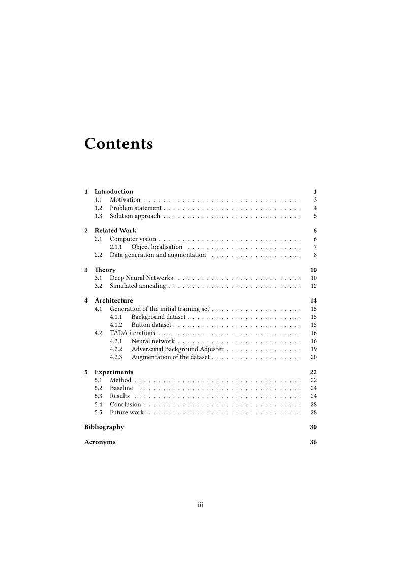
Contents

1 Introduction 11.1 Motivation . . . . . . . . . . . . . . . . . . . . . . . . . . . . . . . . . 31.2 Problem statement . . . . . . . . . . . . . . . . . . . . . . . . . . . . . 41.3 Solution approach . . . . . . . . . . . . . . . . . . . . . . . . . . . . . 5

2 Related Work 62.1 Computer vision . . . . . . . . . . . . . . . . . . . . . . . . . . . . . . 6

2.1.1 Object localisation . . . . . . . . . . . . . . . . . . . . . . . . 72.2 Data generation and augmentation . . . . . . . . . . . . . . . . . . . 8

3 �eory 103.1 Deep Neural Networks . . . . . . . . . . . . . . . . . . . . . . . . . . 103.2 Simulated annealing . . . . . . . . . . . . . . . . . . . . . . . . . . . . 12

4 Architecture 144.1 Generation of the initial training set . . . . . . . . . . . . . . . . . . . 15

4.1.1 Background dataset . . . . . . . . . . . . . . . . . . . . . . . . 154.1.2 Bu�on dataset . . . . . . . . . . . . . . . . . . . . . . . . . . . 15

4.2 TADA iterations . . . . . . . . . . . . . . . . . . . . . . . . . . . . . . 164.2.1 Neural network . . . . . . . . . . . . . . . . . . . . . . . . . . 164.2.2 Adversarial Background Adjuster . . . . . . . . . . . . . . . . 194.2.3 Augmentation of the dataset . . . . . . . . . . . . . . . . . . . 20

5 Experiments 225.1 Method . . . . . . . . . . . . . . . . . . . . . . . . . . . . . . . . . . . 225.2 Baseline . . . . . . . . . . . . . . . . . . . . . . . . . . . . . . . . . . 245.3 Results . . . . . . . . . . . . . . . . . . . . . . . . . . . . . . . . . . . 245.4 Conclusion . . . . . . . . . . . . . . . . . . . . . . . . . . . . . . . . . 285.5 Future work . . . . . . . . . . . . . . . . . . . . . . . . . . . . . . . . 28

Bibliography 30

Acronyms 36

iii

1 | Introduction

�e human visual system is good at localising objects, for computers this is still not atrivial task. Inspired by the neurons in the human brain, Arti�cial Neural Networks(ANNs) were invented to bring the learning power of biological life to computers.�ough initial models of neurons were developed in the mid-twentieth century [MP43,Ros58] it was not until the last decade that ANNs have become e�ective. Be�er networkdesigns, large datasets and the vast increase in computational capabilities of GraphicsProcessing Units (GPUs) improved the performance of ANNs enough to surpass themanually designed computer vision algorithms. �ose algorithms use handcra�edrules to transform the data to another representation, a process called feature extraction.Handcra�ed rules extract features like edges and gradients from images that can thenbe used for further processing to get the desired outcome. �e algorithm is thenprecisely designed to work well for that task. When the task changes, one needs toredesign the whole algorithm. With ANNs, there is no need to precisely de�ne how toextract relevant features from the data. �is is done by a learning procedure. In theprocess of supervised learning, a signi�cant number of inputs and desired outputs froma training set are passed through the network. With enough data, the network is ableto learn by itself what features are relevant to produce the desired output.

�e need for handcra�ing designs is not completely gone with ANNs. �e structureof the network and the learning procedure still need to be adapted to the problemat hand. Because the features themselves are learned, the design task moves to afundamentally higher level of abstraction. Instead of designing algorithms to extractfeatures, the network structure and learning procedure need to be adapted. Existingnetwork structures and learning parameters can be used as a starting point and adaptedto similar tasks. For example, Convolutional Neural Networks (ConvNets) are a specialtype of ANNs and have shown to work well on images, speech and text [KSH12,DYDA12, HZRS15, CW08].

A common task in computer vision is object localisation. Given an image, the task isto annotate the image with the location of an object. ConvNets have been successfullyapplied to the task of object localisation, e.g. [GDDM14, SEZ+14, SZ15, STE13]. AConvNet can be trained end-to-end; that is directly from the raw pixels to the de-sired result. For object localisation, the desired result could be designed as a binarymask [STE13]. �e binary mask annotates the image with the information of whichpixels belong to the object and which pixels do not belong to the object. �e trainingset needs to be su�ciently large and representative for the context the trained networkwill be used in. �e training set contains the images, associated with their correctbinary mask, the ground truth.

1

As ANNs learn to detect the relevant features for the task, the dataset they learnfrom needs to be carefully constructed. In an object localisation task, it is importantthat the neural network learns to localise the object itself without depending on thebackground. If the background in the training set is always white, the network maylearn to rely on the white pixels to decide which pixels are part of the object to localise.�e network will then generalise poorly to other contexts because there might not bea white background around the object.

In this thesis, a novel method is developed which adjusts the background of objectsin the training set to improve the performance of a ConvNet on not previously seenbackgrounds. In our method, the neural network is trained on a trivial background thatis easy to obtain. �e training set is expanded by generating backgrounds speci�callyfor the trained neural network, eliminating the need to manually design a model forthe background.

�e remainder of this chapter will brie�y describe the motivation behind this thesis,introduce our problem statement and describe our proposed solution at a conceptuallevel. Chapter 2 discusses related work regarding object localisation in images and thegeneration of training data. Section 3.1 explains the basics of Deep Neural Networks(DNNs). Readers familiar with DNNs can safely skip this section. Section 3.2 explainsthe details of the optimisation method that will be used in Chapter 4. Chapter 4extends the proposed method by describing precisely which choices we made. �echapter also describes our experimental set-up: how we constructed our dataset, whichnetwork structure we used and how we generate backgrounds. Chapter 5 describes theexperiment around our proposed solution and discusses the results that we obtained.�is chapter also concludes our work and points to ideas for further research.

2

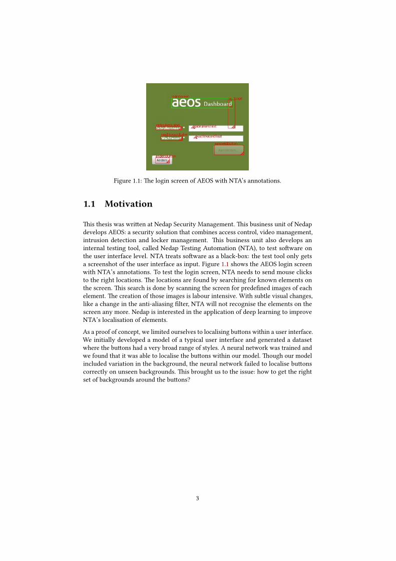
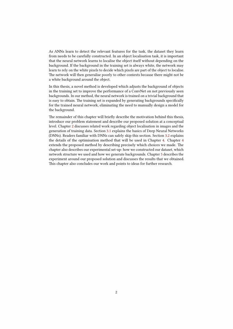
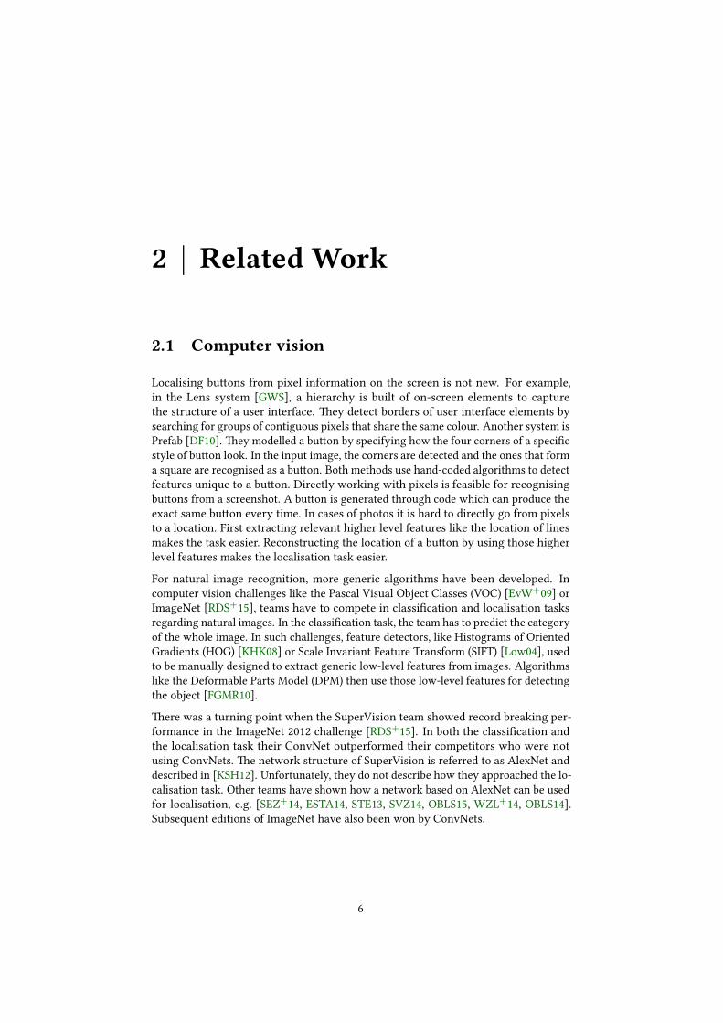
Figure 1.1: �e login screen of AEOS with NTA’s annotations.

1.1 Motivation

�is thesis was wri�en at Nedap Security Management. �is business unit of Nedapdevelops AEOS: a security solution that combines access control, video management,intrusion detection and locker management. �is business unit also develops aninternal testing tool, called Nedap Testing Automation (NTA), to test so�ware onthe user interface level. NTA treats so�ware as a black-box: the test tool only getsa screenshot of the user interface as input. Figure 1.1 shows the AEOS login screenwith NTA’s annotations. To test the login screen, NTA needs to send mouse clicksto the right locations. �e locations are found by searching for known elements onthe screen. �is search is done by scanning the screen for prede�ned images of eachelement. �e creation of those images is labour intensive. With subtle visual changes,like a change in the anti-aliasing �lter, NTA will not recognise the elements on thescreen any more. Nedap is interested in the application of deep learning to improveNTA’s localisation of elements.

As a proof of concept, we limited ourselves to localising bu�ons within a user interface.We initially developed a model of a typical user interface and generated a datasetwhere the bu�ons had a very broad range of styles. A neural network was trained andwe found that it was able to localise the bu�ons within our model. �ough our modelincluded variation in the background, the neural network failed to localise bu�onscorrectly on unseen backgrounds. �is brought us to the issue: how to get the rightset of backgrounds around the bu�ons?

3

Fz6Y1t9EwL

ButtonProperties (label text, possible background colours,max width, etc.) are speci�ed by the model

BackgroundCould be anything

SampleInput to the neural network

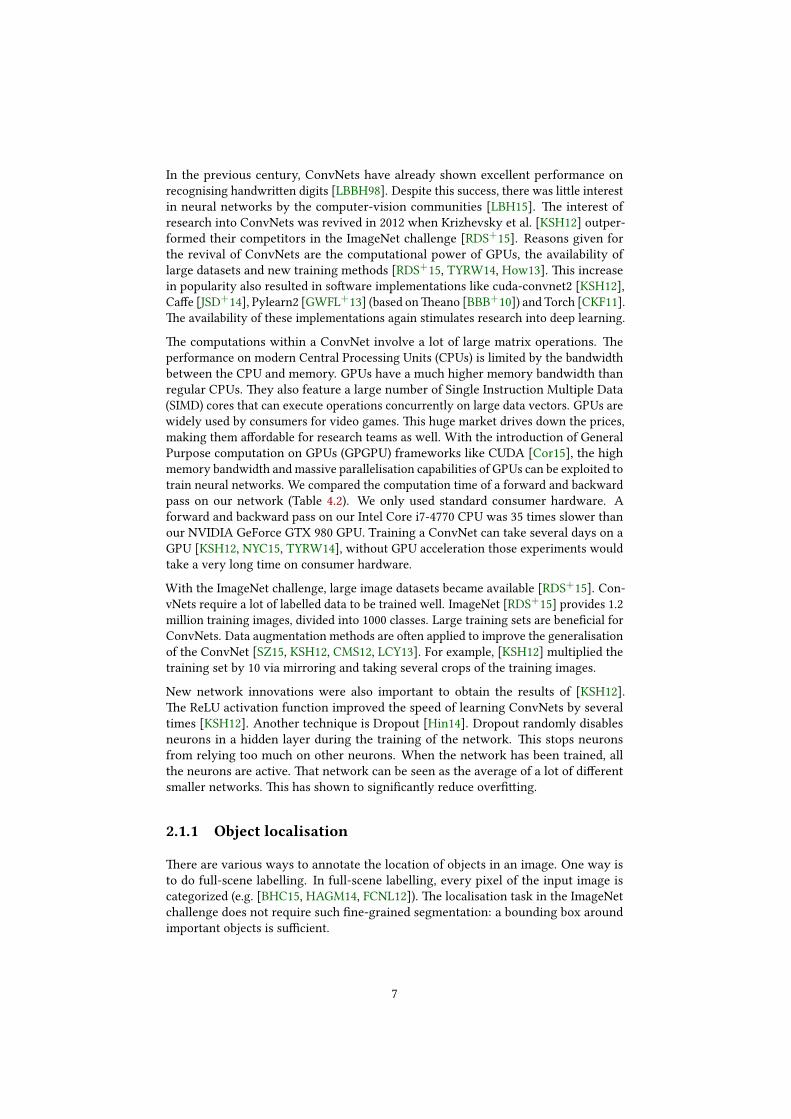
Figure 1.2: Overview of the bu�on localisation task.

1.2 Problem statement

In this thesis we want to localise a bu�on from a single web application. Within anapplication, bu�ons usually have the same design (e.g. always square and a borderaround it) but still vary in properties (e.g. like their text content, size and colour). Wecreated a model of a bu�on that represents one speci�c bu�on style. �e idea behindthis model is that it captures enough variation to let the neural network localise allthe bu�ons that comply to the design speci�ed by our model.

Since ConvNets have shown to work well on images, we want to use their learningpower to learn to localise bu�ons in a screenshot. We do not want to resort todesigning handcra�ed algorithms. With a model of the bu�on, we can generate asu�cient number of bu�ons for the training set. When the trained network is appliedin practice, it will have to localise the bu�ons of the speci�c web application the modelwas designed for. When it encounters such a bu�on, it has already seen a similarone in the training set. �e network should have learned to correctly localise thatbu�on. On the other hand, we do not have a model that describes the backgrounds theneural network will encounter. �e environment around the bu�on could be anything.Training the network on every possible background is infeasible as the number ofpossible backgrounds scales exponentially with the number of pixels. Somehow weneed to make sure the neural network can learn to recognise the bu�on without relyingon the background around it. Figure 1.2 shows an overview of the bu�on localisationtask.

4

TADA iterations

Train CNN

Augment training set

Adversarial Background Adjuster

Initial training set

Final CNN

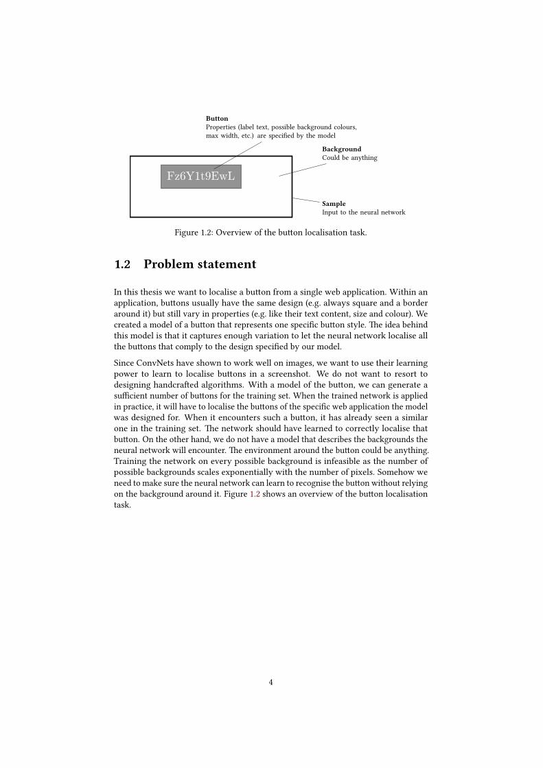
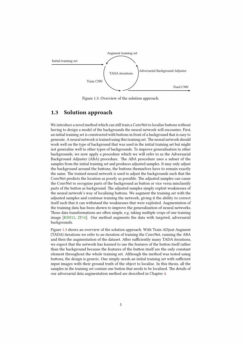
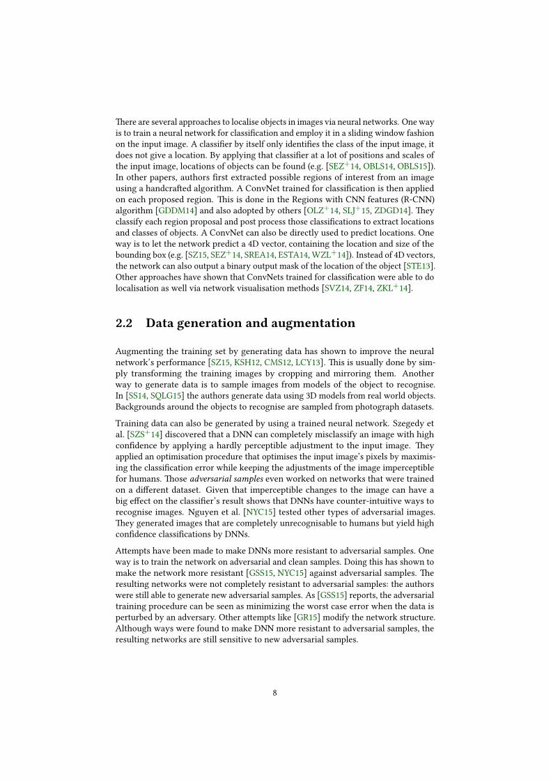
Figure 1.3: Overview of the solution approach.

1.3 Solution approach

We introduce a novel method which can still train a ConvNet to localise bu�ons withouthaving to design a model of the backgrounds the neural network will encounter. First,an initial training set is constructed with bu�ons in front of a background that is easy togenerate. A neural network is trained using this training set. �e neural network shouldwork well on the type of background that was used in the initial training set but mightnot generalise well to other types of backgrounds. To improve generalisation to otherbackgrounds, we now apply a procedure which we will refer to as the AdversarialBackground Adjuster (ABA) procedure. �e ABA procedure uses a subset of thesamples from the initial training set and produces adjusted samples. It may only adjustthe background around the bu�ons, the bu�ons themselves have to remain exactlythe same. �e trained neural network is used to adjust the backgrounds such that theConvNet predicts the location as poorly as possible. �e adjusted samples can causethe ConvNet to recognise parts of the background as bu�on or vice versa misclassifyparts of the bu�on as background. �e adjusted samples simply exploit weaknesses ofthe neural network’s way of localising bu�ons. We augment the training set with theadjusted samples and continue training the network, giving it the ability to correctitself such that it can withstand the weaknesses that were exploited. Augmentation ofthe training data has been shown to improve the generalisation of neural networks.�ose data transformations are o�en simple, e.g. taking multiple crops of one trainingimage [KSH12, ZF14]. Our method augments the data with targeted, adversarialbackgrounds.

Figure 1.3 shows an overview of the solution approach. With Train ADjust Augment(TADA) iterations we refer to an iteration of training the ConvNet, running the ABAand then the augmentation of the dataset. A�er su�ciently many TADA iterations,we expect that the network has learned to use the features of the bu�on itself ratherthan the background because the features of the bu�on itself are the only constantelement throughout the whole training set. Although the method was tested usingbu�ons, the design is generic. One simply needs an initial training set with su�cientinput images with their ground truth of the object to localise. In this thesis, all thesamples in the training set contain one bu�on that needs to be localised. �e details ofour adversarial data augmentation method are described in Chapter 4.

5

2 | Related Work

2.1 Computer vision

Localising bu�ons from pixel information on the screen is not new. For example,in the Lens system [GWS], a hierarchy is built of on-screen elements to capturethe structure of a user interface. �ey detect borders of user interface elements bysearching for groups of contiguous pixels that share the same colour. Another system isPrefab [DF10]. �ey modelled a bu�on by specifying how the four corners of a speci�cstyle of bu�on look. In the input image, the corners are detected and the ones that forma square are recognised as a bu�on. Both methods use hand-coded algorithms to detectfeatures unique to a bu�on. Directly working with pixels is feasible for recognisingbu�ons from a screenshot. A bu�on is generated through code which can produce theexact same bu�on every time. In cases of photos it is hard to directly go from pixelsto a location. First extracting relevant higher level features like the location of linesmakes the task easier. Reconstructing the location of a bu�on by using those higherlevel features makes the localisation task easier.

For natural image recognition, more generic algorithms have been developed. Incomputer vision challenges like the Pascal Visual Object Classes (VOC) [EvW+09] orImageNet [RDS+15], teams have to compete in classi�cation and localisation tasksregarding natural images. In the classi�cation task, the team has to predict the categoryof the whole image. In such challenges, feature detectors, like Histograms of OrientedGradients (HOG) [KHK08] or Scale Invariant Feature Transform (SIFT) [Low04], usedto be manually designed to extract generic low-level features from images. Algorithmslike the Deformable Parts Model (DPM) then use those low-level features for detectingthe object [FGMR10].

�ere was a turning point when the SuperVision team showed record breaking per-formance in the ImageNet 2012 challenge [RDS+15]. In both the classi�cation andthe localisation task their ConvNet outperformed their competitors who were notusing ConvNets. �e network structure of SuperVision is referred to as AlexNet anddescribed in [KSH12]. Unfortunately, they do not describe how they approached the lo-calisation task. Other teams have shown how a network based on AlexNet can be usedfor localisation, e.g. [SEZ+14, ESTA14, STE13, SVZ14, OBLS15, WZL+14, OBLS14].Subsequent editions of ImageNet have also been won by ConvNets.

6

In the previous century, ConvNets have already shown excellent performance onrecognising handwri�en digits [LBBH98]. Despite this success, there was li�le interestin neural networks by the computer-vision communities [LBH15]. �e interest ofresearch into ConvNets was revived in 2012 when Krizhevsky et al. [KSH12] outper-formed their competitors in the ImageNet challenge [RDS+15]. Reasons given forthe revival of ConvNets are the computational power of GPUs, the availability oflarge datasets and new training methods [RDS+15, TYRW14, How13]. �is increasein popularity also resulted in so�ware implementations like cuda-convnet2 [KSH12],Ca�e [JSD+14], Pylearn2 [GWFL+13] (based on �eano [BBB+10]) and Torch [CKF11].�e availability of these implementations again stimulates research into deep learning.

�e computations within a ConvNet involve a lot of large matrix operations. �eperformance on modern Central Processing Units (CPUs) is limited by the bandwidthbetween the CPU and memory. GPUs have a much higher memory bandwidth thanregular CPUs. �ey also feature a large number of Single Instruction Multiple Data(SIMD) cores that can execute operations concurrently on large data vectors. GPUs arewidely used by consumers for video games. �is huge market drives down the prices,making them a�ordable for research teams as well. With the introduction of GeneralPurpose computation on GPUs (GPGPU) frameworks like CUDA [Cor15], the highmemory bandwidth and massive parallelisation capabilities of GPUs can be exploited totrain neural networks. We compared the computation time of a forward and backwardpass on our network (Table 4.2). We only used standard consumer hardware. Aforward and backward pass on our Intel Core i7-4770 CPU was 35 times slower thanour NVIDIA GeForce GTX 980 GPU. Training a ConvNet can take several days on aGPU [KSH12, NYC15, TYRW14], without GPU acceleration those experiments wouldtake a very long time on consumer hardware.

With the ImageNet challenge, large image datasets became available [RDS+15]. Con-vNets require a lot of labelled data to be trained well. ImageNet [RDS+15] provides 1.2million training images, divided into 1000 classes. Large training sets are bene�cial forConvNets. Data augmentation methods are o�en applied to improve the generalisationof the ConvNet [SZ15, KSH12, CMS12, LCY13]. For example, [KSH12] multiplied thetraining set by 10 via mirroring and taking several crops of the training images.

New network innovations were also important to obtain the results of [KSH12].�e ReLU activation function improved the speed of learning ConvNets by severaltimes [KSH12]. Another technique is Dropout [Hin14]. Dropout randomly disablesneurons in a hidden layer during the training of the network. �is stops neuronsfrom relying too much on other neurons. When the network has been trained, allthe neurons are active. �at network can be seen as the average of a lot of di�erentsmaller networks. �is has shown to signi�cantly reduce over��ing.

2.1.1 Object localisation

�ere are various ways to annotate the location of objects in an image. One way isto do full-scene labelling. In full-scene labelling, every pixel of the input image iscategorized (e.g. [BHC15, HAGM14, FCNL12]). �e localisation task in the ImageNetchallenge does not require such �ne-grained segmentation: a bounding box aroundimportant objects is su�cient.

7

�ere are several approaches to localise objects in images via neural networks. One wayis to train a neural network for classi�cation and employ it in a sliding window fashionon the input image. A classi�er by itself only identi�es the class of the input image, itdoes not give a location. By applying that classi�er at a lot of positions and scales ofthe input image, locations of objects can be found (e.g. [SEZ+14, OBLS14, OBLS15]).In other papers, authors �rst extracted possible regions of interest from an imageusing a handcra�ed algorithm. A ConvNet trained for classi�cation is then appliedon each proposed region. �is is done in the Regions with CNN features (R-CNN)algorithm [GDDM14] and also adopted by others [OLZ+14, SLJ+15, ZDGD14]. �eyclassify each region proposal and post process those classi�cations to extract locationsand classes of objects. A ConvNet can also be directly used to predict locations. Oneway is to let the network predict a 4D vector, containing the location and size of thebounding box (e.g. [SZ15, SEZ+14, SREA14, ESTA14, WZL+14]). Instead of 4D vectors,the network can also output a binary output mask of the location of the object [STE13].Other approaches have shown that ConvNets trained for classi�cation were able to dolocalisation as well via network visualisation methods [SVZ14, ZF14, ZKL+14].

2.2 Data generation and augmentation

Augmenting the training set by generating data has shown to improve the neuralnetwork’s performance [SZ15, KSH12, CMS12, LCY13]. �is is usually done by sim-ply transforming the training images by cropping and mirroring them. Anotherway to generate data is to sample images from models of the object to recognise.In [SS14, SQLG15] the authors generate data using 3D models from real world objects.Backgrounds around the objects to recognise are sampled from photograph datasets.

Training data can also be generated by using a trained neural network. Szegedy etal. [SZS+14] discovered that a DNN can completely misclassify an image with highcon�dence by applying a hardly perceptible adjustment to the input image. �eyapplied an optimisation procedure that optimises the input image’s pixels by maximis-ing the classi�cation error while keeping the adjustments of the image imperceptiblefor humans. �ose adversarial samples even worked on networks that were trainedon a di�erent dataset. Given that imperceptible changes to the image can have abig e�ect on the classi�er’s result shows that DNNs have counter-intuitive ways torecognise images. Nguyen et al. [NYC15] tested other types of adversarial images.�ey generated images that are completely unrecognisable to humans but yield highcon�dence classi�cations by DNNs.

A�empts have been made to make DNNs more resistant to adversarial samples. Oneway is to train the network on adversarial and clean samples. Doing this has shown tomake the network more resistant [GSS15, NYC15] against adversarial samples. �eresulting networks were not completely resistant to adversarial samples: the authorswere still able to generate new adversarial samples. As [GSS15] reports, the adversarialtraining procedure can be seen as minimizing the worst case error when the data isperturbed by an adversary. Other a�empts like [GR15] modify the network structure.Although ways were found to make DNN more resistant to adversarial samples, theresulting networks are still sensitive to new adversarial samples.

8

Instead of using existing datasets to use as backgrounds like in [SS14, SQLG15], wegenerate the backgrounds ourselves. �e bu�ons we would like to recognise livein a digital environment instead of a natural environment. �e screenshots fromuser interfaces simply do not look like photos from the real world. It is not trivial tomanually develop a model of this environment to generate backgrounds. �e absence ofa model of the background is resolved by employing the power of adversarial samplesto automatically produce backgrounds. �e adversarial backgrounds are speci�callytargeted towards our trained neural network. In contrast to [GSS15, NYC15, GR15],we do not give the adversary complete control over all the pixels. In our situationthe adversary may only adjust pixels that are not part of the bu�on that needs to belocalised.

9

3 | �eory

3.1 Deep Neural Networks

DNNs are based on a lot of simple processors, called neurons. �ey are inspired by abiological brain in the hope to bring their learning capability to computers. We willbrie�y present some theory for a basic understanding of their workings. More detailscan be found in resources about neural network theory, e.g. [LBH15, Hay99, Sch15].

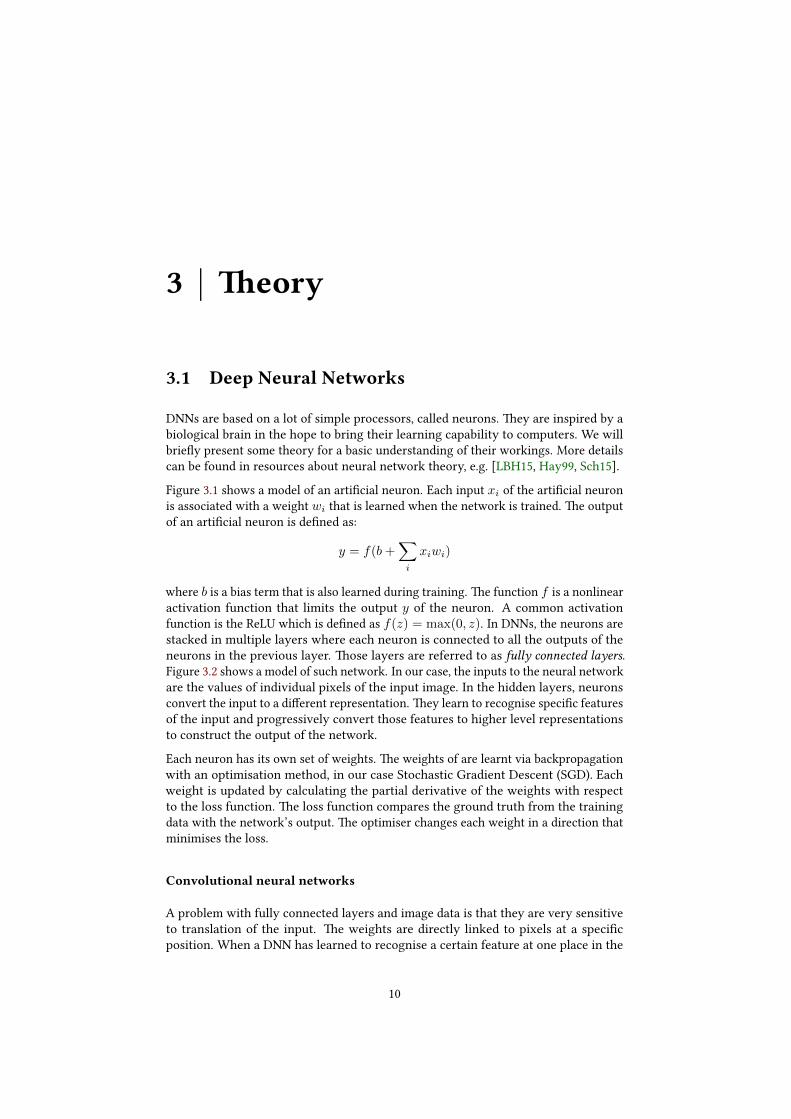
Figure 3.1 shows a model of an arti�cial neuron. Each input xi of the arti�cial neuronis associated with a weight wi that is learned when the network is trained. �e outputof an arti�cial neuron is de�ned as:

y = f(b+∑

i

xiwi)

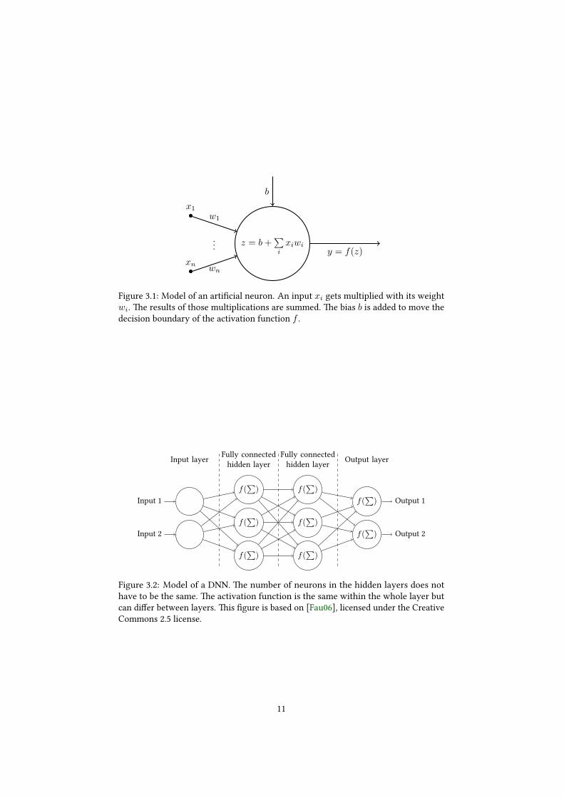
where b is a bias term that is also learned during training. �e function f is a nonlinearactivation function that limits the output y of the neuron. A common activationfunction is the ReLU which is de�ned as f(z) = max(0, z). In DNNs, the neurons arestacked in multiple layers where each neuron is connected to all the outputs of theneurons in the previous layer. �ose layers are referred to as fully connected layers.Figure 3.2 shows a model of such network. In our case, the inputs to the neural networkare the values of individual pixels of the input image. In the hidden layers, neuronsconvert the input to a di�erent representation. �ey learn to recognise speci�c featuresof the input and progressively convert those features to higher level representationsto construct the output of the network.

Each neuron has its own set of weights. �e weights of are learnt via backpropagationwith an optimisation method, in our case Stochastic Gradient Descent (SGD). Eachweight is updated by calculating the partial derivative of the weights with respectto the loss function. �e loss function compares the ground truth from the trainingdata with the network’s output. �e optimiser changes each weight in a direction thatminimises the loss.

Convolutional neural networks

A problem with fully connected layers and image data is that they are very sensitiveto translation of the input. �e weights are directly linked to pixels at a speci�cposition. When a DNN has learned to recognise a certain feature at one place in the

10

z = b+∑i

xiwi

x1

xn

w1

wn

...y = f(z)

b

Figure 3.1: Model of an arti�cial neuron. An input xi gets multiplied with its weightwi. �e results of those multiplications are summed. �e bias b is added to move thedecision boundary of the activation function f .

Input 1

Input 2

f(∑

)

f(∑

)

f(∑

)

f(∑

)

f(∑

)

f(∑

)

f(∑

) Output 1

f(∑

) Output 2

Fully connectedhidden layer

Fully connectedhidden layerInput layer Output layer

Figure 3.2: Model of a DNN. �e number of neurons in the hidden layers does nothave to be the same. �e activation function is the same within the whole layer butcan di�er between layers. �is �gure is based on [Fau06], licensed under the CreativeCommons 2.5 license.

11

623

8

1

48

18

11024

Denseconnections...

33

6

Input Convolutionstride 1

Max Poolingstride 2

Fully connected Output

1

48

18

6

33

46

16

1

1

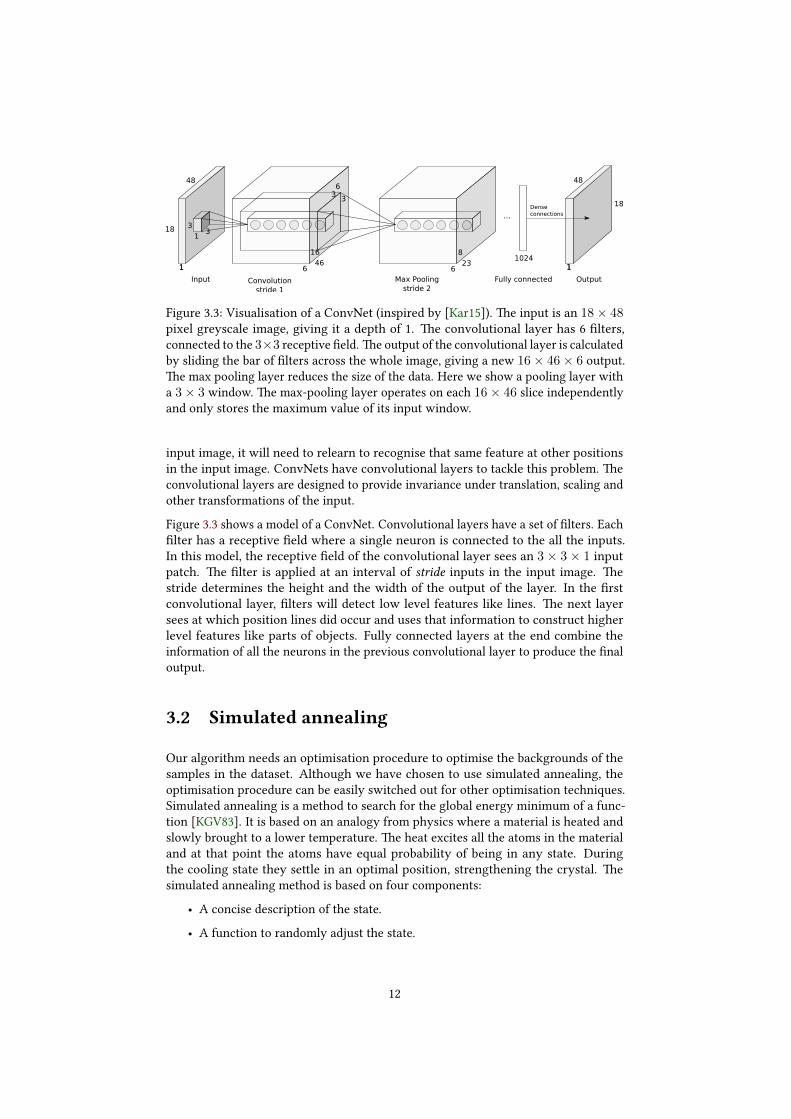
Figure 3.3: Visualisation of a ConvNet (inspired by [Kar15]). �e input is an 18× 48pixel greyscale image, giving it a depth of 1. �e convolutional layer has 6 �lters,connected to the 3×3 receptive �eld. �e output of the convolutional layer is calculatedby sliding the bar of �lters across the whole image, giving a new 16× 46× 6 output.�e max pooling layer reduces the size of the data. Here we show a pooling layer witha 3× 3 window. �e max-pooling layer operates on each 16× 46 slice independentlyand only stores the maximum value of its input window.

input image, it will need to relearn to recognise that same feature at other positionsin the input image. ConvNets have convolutional layers to tackle this problem. �econvolutional layers are designed to provide invariance under translation, scaling andother transformations of the input.

Figure 3.3 shows a model of a ConvNet. Convolutional layers have a set of �lters. Each�lter has a receptive �eld where a single neuron is connected to the all the inputs.In this model, the receptive �eld of the convolutional layer sees an 3 × 3 × 1 inputpatch. �e �lter is applied at an interval of stride inputs in the input image. �estride determines the height and the width of the output of the layer. In the �rstconvolutional layer, �lters will detect low level features like lines. �e next layersees at which position lines did occur and uses that information to construct higherlevel features like parts of objects. Fully connected layers at the end combine theinformation of all the neurons in the previous convolutional layer to produce the �naloutput.

3.2 Simulated annealing

Our algorithm needs an optimisation procedure to optimise the backgrounds of thesamples in the dataset. Although we have chosen to use simulated annealing, theoptimisation procedure can be easily switched out for other optimisation techniques.Simulated annealing is a method to search for the global energy minimum of a func-tion [KGV83]. It is based on an analogy from physics where a material is heated andslowly brought to a lower temperature. �e heat excites all the atoms in the materialand at that point the atoms have equal probability of being in any state. Duringthe cooling state they se�le in an optimal position, strengthening the crystal. �esimulated annealing method is based on four components:

• A concise description of the state.

• A function to randomly adjust the state.

12

• A function to measure the poorness of the state: the loss function.

• An annealing schedule.

Simulated annealing tries to �nd the state for which the loss function gives the lowestoutput. It does so by iterative improvement. �e algorithm starts with an initial state,randomly adjusts it and tests whether the loss of that new state has been improved.It can choose to do a new iteration on this state by randomly adjusting this newlyobtained state again. If it would always do this, the algorithm might get stuck in alocal optimum. Simulated annealing tries to prevent ge�ing stuck in local optima via atemperature, based on the analogy from physics. �e temperature starts o� high and islowered according to the annealing schedule in each iteration. When the temperatureis high, it will accept almost every new state. �e lower the temperature, the lowerthe probability that a worse state is accepted. In each step of the algorithm, the loss Lof the new state is compared with the previous loss. If it is worse (so a higher loss),the new state is accepted when exp(−∆L

T ) ≥ UniformRandomReal(0, 1) holds. Ifthe loss is lower, it is always accepted.

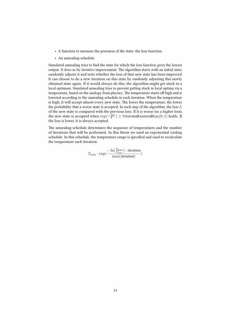
�e annealing schedule determines the sequence of temperatures and the numberof iterations that will be performed. In this thesis we used an exponential coolingschedule. In this schedule, the temperature range is speci�ed and used to recalculatethe temperature each iteration:

Tmax · exp(− ln(Tmax

Tmin) · iteration

max(iteration))

13

4 | Architecture

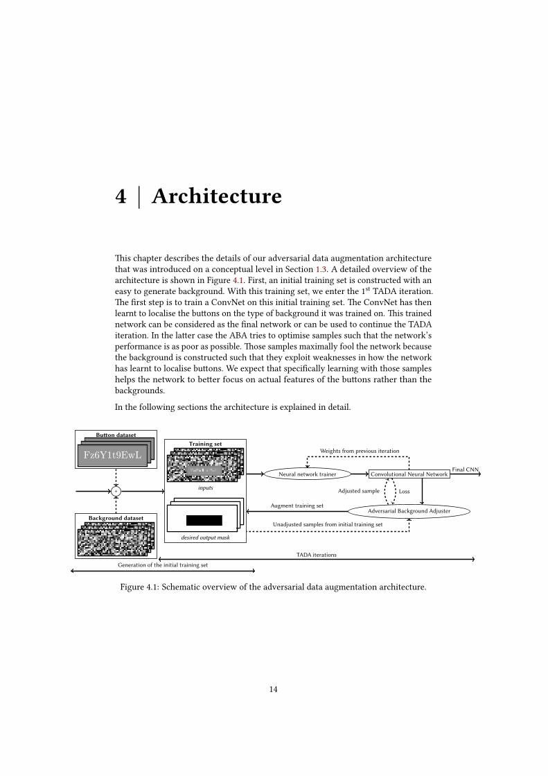
�is chapter describes the details of our adversarial data augmentation architecturethat was introduced on a conceptual level in Section 1.3. A detailed overview of thearchitecture is shown in Figure 4.1. First, an initial training set is constructed with aneasy to generate background. With this training set, we enter the 1st TADA iteration.�e �rst step is to train a ConvNet on this initial training set. �e ConvNet has thenlearnt to localise the bu�ons on the type of background it was trained on. �is trainednetwork can be considered as the �nal network or can be used to continue the TADAiteration. In the la�er case the ABA tries to optimise samples such that the network’sperformance is as poor as possible. �ose samples maximally fool the network becausethe background is constructed such that they exploit weaknesses in how the networkhas learnt to localise bu�ons. We expect that speci�cally learning with those sampleshelps the network to be�er focus on actual features of the bu�ons rather than thebackgrounds.

In the following sections the architecture is explained in detail.

Training set

inputs

desired output mask

+

Bu�on dataset

Fz6Y1t9EwLFz6Y1t9EwLFz6Y1t9EwL

Background dataset

Neural network trainer Convolutional Neural NetworkFinal CNN

Adversarial Background Adjuster

Weights from previous iteration

Adjusted sample Loss

Augment training set

Unadjusted samples from initial training set

Generation of the initial training set

TADA iterations

Figure 4.1: Schematic overview of the adversarial data augmentation architecture.

14

4.1 Generation of the initial training set

�e generation of the initial training set involves two main components: the objectsto localise and the background to put around it. Both the background and bu�on areconverted to greyscale. �e backgrounds have a resolution of 48 × 18 pixels. �ereason for using greyscale (opposed to colour) at a low resolution is to decrease thecomputation time, allowing more experiments to be done in a shorter time frame.

We place the bu�on in front of the background and encode the location of the bu�onas a binary mask. �e mask indicates which pixels belong to the object to localise. �ebu�on is placed at a random location on the background with two restrictions: thewhole bu�on has to �t on that location (no cropping) and the 2 pixel radius aroundthe centre of the background has to be covered by the bu�on. We do this becausehypothetically, the ABA could start drawing actual bu�ons on the background. �epositioning of the bu�on to localise is a unique property that allows the network todistinguish the bu�on to localise from potential bu�ons generated by the ABA. Inthe case that the ABA has drawn actual bu�ons on the background, those bu�onsstill miss the unique property. Without this restriction the ABA has the freedom todraw bu�ons that are indistinguishable from the original bu�on to localise. We wouldthen punish the network for recognising an actual bu�on. �e unique property simplyprevents this situation from occurring because the network should only detect bu�onswith the unique property.

With the model of the object we can create a training set of any arbitrary size. We do notreuse bu�ons or backgrounds in the initial training set. In initial experiments, we foundthat 38000 frames of a NOS (Nederlandse Omroep Stichting, English: Dutch BroadcastFoundation) news broadcast as background was su�cient to obtain a network thatperformed well on another NOS news broadcast as background. Due to this result, thelength of the initial training set was set to 38000 samples with a white background.We did not test with other dataset sizes.

4.1.1 Background dataset

�e initial training set is constructed with a background that is completely white.A�er the �nal ConvNet has been trained, it could encounter any background. Withthe completely white background, the neural network can easily localise bu�ons byclassifying non-white areas to be part of the bu�on. We rely on the ABA to properlyoptimise the backgrounds, preventing the need to construct a representative model ofthe backgrounds the neural network will encounter.

4.1.2 Button dataset

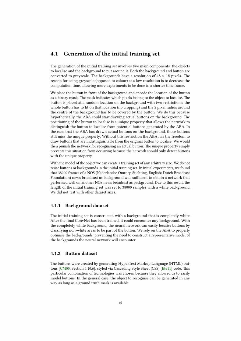
�e bu�ons were created by generating HyperText Markup Language (HTML) but-tons [CM00, Section 4.10.6], styled via Cascading Style Sheet (CSS) [Ete11] code. �isparticular combination of technologies was chosen because they allowed us to easilymodel bu�ons. In the general case, the object to recognise can be generated in anyway as long as a ground truth mask is available.

15

CSS property Valuebackground UniformRandomInteger(50, 200) for each RGB colour

channelborder-color 0.8 · background(text) color #FFF

border-width 2px

min-width UniformRandomInteger(3, 10) · 10pxpadding UniformRandomChoice({5px, 10px})font-family UniformRandomChoice({Andale Mono, Arial,

Arial Black, cmmi10, cmr10, Comic Sans MS,DejaVu Sans, eufm10, Impact})

Table 4.1: CSS properties used to generate bu�ons.

�e bu�ons are characterised by having a solid background with a slightly darkerborder around it, see Figure 4.1. Table 4.1 shows the CSS properties that were usedwith their possible values. Variation of the style of the bu�on was done to makethe localisation task less trivial. �e bu�on is �lled with a random text by randomlysampling from a uniform distribution of le�ers (a-z, upper-case and lower-case), digitsand spaces. �e length of the random text was at least 2 characters and at most 10characters. �e length of the text also in�uences the width of the bu�on. Bu�ons werescaled to 12.5% of their size, rounding to complete pixels. �e downscaling is neededto let the bu�ons �t within the 48× 18 pixel input resolution of the neural network.�e average bu�on covers 22% of this area.

4.2 TADA iterations

4.2.1 Neural network

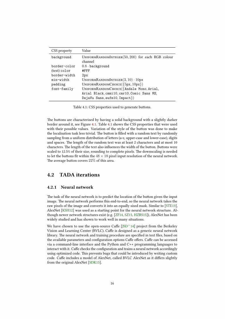
�e task of the neural network is to predict the location of the bu�on given the inputimage. �e neural network performs this end-to-end, so the neural network takes theraw pixels of the image and converts it into an equally sized mask. Similar to [STE13],AlexNet [KSH12] was used as a starting point for the neural network structure. Al-though newer network structures exist (e.g. [ZF14, SZ15, HZRS15]), AlexNet has beenwidely studied and has shown to work well in many situations.

We have chosen to use the open-source Ca�e [JSD+14] project from the BerkeleyVision and Learning Center (BVLC). Ca�e is designed as a generic neural networklibrary. �e neural network and training procedure are speci�ed in text �les, based onthe available parameters and con�guration options Ca�e o�ers. Ca�e can be accessedvia a command-line interface and the Python and C++ programming languages tointeract with it. Ca�e checks the con�guration and trains a neural network accordinglyusing optimized code. �is prevents bugs that could be introduced by writing customcode. Ca�e includes a model of AlexNet, called BVLC AlexNet as it di�ers slightlyfrom the original AlexNet [SDK15].

16

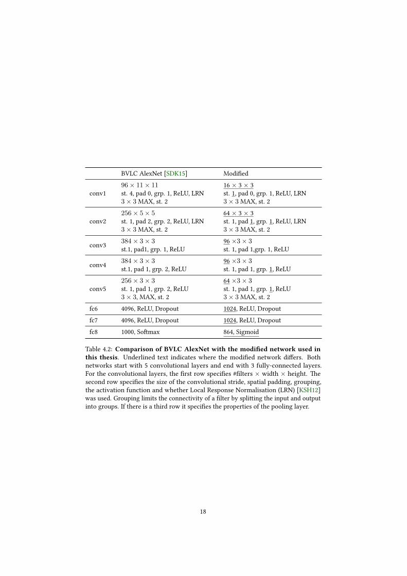
Table 4.2 shows an overview of the layers in the original and the modi�ed networkwe used. For more details about the network structure, see [KSH12]. �e originalAlexNet network was designed for assigning a single class to an image. We optimisedthe network for our localisation task, the most notable changes are:

• �e input resolution was lowered from 3×244×244 to 1×48×18 as describedin Section 4.1.

• �e �nal activation function was changed from a so�max to sigmoid function.

• �e number of �lters in the convolutional layers and units in the fully connectedlayers were lowered. By visualising and experimentally lowering the number of�lters in layers we observed that the computational complexity of the networkcould be reduced without lowering its classi�cation performance too much.

• No spli�ing of convolutional layers (grouping). In the original AlexNet, someconvolutional layers were split across two GPUs due to memory constraints.Some of those layers only communicated with the preceding layer on that GPU.Our hardware had enough available GPU memory so we did not need to usegrouping.

�e original network had a so�max as �nal activation function. �e so�max functionensures that the output is a probability distribution over all the classes: the sum overall the outputs is 1. In our localisation task, similar to [STE13], we want to predict afull binary mask. �e activation function in the last layer of the network cannot bea threshold function because the backpropagation algorithm requires di�erentiablefunctions [Hay99, Section 1.3]. A common activation function is the sigmoid func-tion, de�ned by f(x) = 1

1+e−x . �is is a continuous, di�erentiable function withlimx→∞

f(x) = 1 and limx→−∞

f(x) = 0. A�er learning, a threshold t ∈ (0, 1) can beapplied to the output of the sigmoid function to convert the network’s output to binary.

We lowered the size of the �lters in the �rst layer from 11×11 to 3×3. With our lowerresolution input we lower the size of the convolutional �lters with it. To preservemore detail for our localisation task, the stride was changed from 4 to 1. Zeiler andFergus [ZF14] found that lowering the �lter size and the stride of the �rst layer helpedretaining more information in the 1st and 2nd layer. Simonyan and Zisserman [SZ15]showed even be�er performance by using 3× 3 �lters with stride 1 throughout thewhole network. We observed that the number of �lters could be lowered withoutlowering its classi�cation performance too much.

�e pooling layers remove spatial details by reducing the width and height of aconvolutional layer. Dosovitskiy and Brox [DB15] have reconstructed images basedon feature activations of AlexNet and found that object positions are preserved in theconvolutional layers. Our experiments also show that this network structure is able tolocalise objects with high accuracy and recall.

�is network structure needs to be trained. �e learning parameters are based on theparameters included in BVLC’s AlexNet model [SDK15], see Table 4.3. Most parametersare constant for every TADA iteration, only the learning rate at start and the numberof samples in the training set changes.

17

BVLC AlexNet [SDK15] Modi�ed96× 11× 11 16 × 3 × 3

conv1 st. 4, pad 0, grp. 1, ReLU, LRN st. 1, pad 0, grp. 1, ReLU, LRN3× 3 MAX, st. 2 3× 3 MAX, st. 2256× 5× 5 64 × 3 × 3

conv2 st. 1, pad 2, grp. 2, ReLU, LRN st. 1, pad 1, grp. 1, ReLU, LRN3× 3 MAX, st. 2 3× 3 MAX, st. 2

conv3 384× 3× 3 96 ×3× 3st.1, pad1, grp. 1, ReLU st. 1, pad 1,grp. 1, ReLU

conv4 384× 3× 3 96 ×3× 3st.1, pad 1, grp. 2, ReLU st. 1, pad 1, grp. 1, ReLU256× 3× 3 64 ×3× 3

conv5 st. 1, pad 1, grp. 2, ReLU st. 1, pad 1, grp. 1, ReLU3× 3, MAX, st. 2 3× 3 MAX, st. 2

fc6 4096, ReLU, Dropout 1024, ReLU, Dropoutfc7 4096, ReLU, Dropout 1024, ReLU, Dropoutfc8 1000, So�max 864, Sigmoid

Table 4.2: Comparison of BVLC AlexNet with the modi�ed network used inthis thesis. Underlined text indicates where the modi�ed network di�ers. Bothnetworks start with 5 convolutional layers and end with 3 fully-connected layers.For the convolutional layers, the �rst row speci�es #�lters × width × height. �esecond row speci�es the size of the convolutional stride, spatial padding, grouping,the activation function and whether Local Response Normalisation (LRN) [KSH12]was used. Grouping limits the connectivity of a �lter by spli�ing the input and outputinto groups. If there is a third row it speci�es the properties of the pooling layer.

18

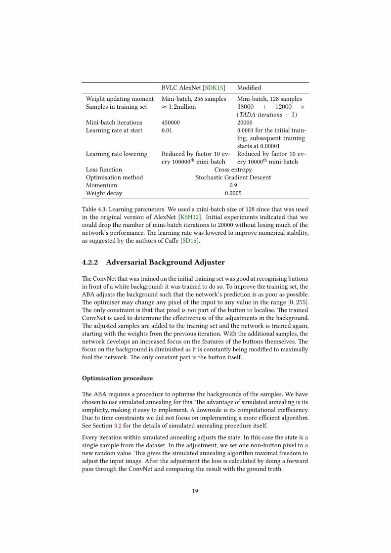
BVLC AlexNet [SDK15] Modi�edWeight updating moment Mini-batch, 256 samples Mini-batch, 128 samplesSamples in training set ≈ 1.2million 38000 + 12000 ×

(TADA-iterations − 1)Mini-batch iterations 450000 20000Learning rate at start 0.01 0.0001 for the initial train-

ing, subsequent trainingstarts at 0.00001

Learning rate lowering Reduced by factor 10 ev-ery 100000th mini-batch

Reduced by factor 10 ev-ery 10000th mini-batch

Loss function Cross entropyOptimisation method Stochastic Gradient DescentMomentum 0.9Weight decay 0.0005

Table 4.3: Learning parameters. We used a mini-batch size of 128 since that was usedin the original version of AlexNet [KSH12]. Initial experiments indicated that wecould drop the number of mini-batch iterations to 20000 without losing much of thenetwork’s performance. �e learning rate was lowered to improve numerical stability,as suggested by the authors of Ca�e [SD15].

4.2.2 Adversarial Background Adjuster

�e ConvNet that was trained on the initial training set was good at recognising bu�onsin front of a white background: it was trained to do so. To improve the training set, theABA adjusts the background such that the network’s prediction is as poor as possible.�e optimiser may change any pixel of the input to any value in the range [0, 255].�e only constraint is that that pixel is not part of the bu�on to localise. �e trainedConvNet is used to determine the e�ectiveness of the adjustments in the background.�e adjusted samples are added to the training set and the network is trained again,starting with the weights from the previous iteration. With the additional samples, thenetwork develops an increased focus on the features of the bu�ons themselves. �efocus on the background is diminished as it is constantly being modi�ed to maximallyfool the network. �e only constant part is the bu�on itself.

Optimisation procedure

�e ABA requires a procedure to optimise the backgrounds of the samples. We havechosen to use simulated annealing for this. �e advantage of simulated annealing is itssimplicity, making it easy to implement. A downside is its computational ine�ciency.Due to time constraints we did not focus on implementing a more e�cient algorithm.See Section 3.2 for the details of simulated annealing procedure itself.

Every iteration within simulated annealing adjusts the state. In this case the state is asingle sample from the dataset. In the adjustment, we set one non-bu�on pixel to anew random value. �is gives the simulated annealing algorithm maximal freedom toadjust the input image. A�er the adjustment the loss is calculated by doing a forwardpass through the ConvNet and comparing the result with the ground truth.

19

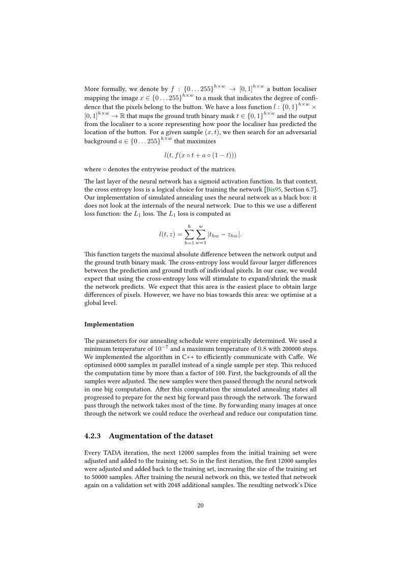
More formally, we denote by f : {0 . . . 255}h×w → [0, 1]h×w a bu�on localiser

mapping the image x ∈ {0 . . . 255}h×w to a mask that indicates the degree of con�-dence that the pixels belong to the bu�on. We have a loss function l : {0, 1}h×w ×[0, 1]

h×w → R that maps the ground truth binary mask t ∈ {0, 1}h×w and the outputfrom the localiser to a score representing how poor the localiser has predicted thelocation of the bu�on. For a given sample (x, t), we then search for an adversarialbackground a ∈ {0 . . . 255}h×w that maximizes

l(t, f(x ◦ t+ a ◦ (1− t)))

where ◦ denotes the entrywise product of the matrices.

�e last layer of the neural network has a sigmoid activation function. In that context,the cross entropy loss is a logical choice for training the network [Bis95, Section 6.7].Our implementation of simulated annealing uses the neural network as a black box: itdoes not look at the internals of the neural network. Due to this we use a di�erentloss function: the L1 loss. �e L1 loss is computed as

l(t, z) =

h∑

h=1

w∑

w=1

|thw − zhw|.

�is function targets the maximal absolute di�erence between the network output andthe ground truth binary mask. �e cross-entropy loss would favour larger di�erencesbetween the prediction and ground truth of individual pixels. In our case, we wouldexpect that using the cross-entropy loss will stimulate to expand/shrink the maskthe network predicts. We expect that this area is the easiest place to obtain largedi�erences of pixels. However, we have no bias towards this area: we optimise at aglobal level.

Implementation

�e parameters for our annealing schedule were empirically determined. We used aminimum temperature of 10−7 and a maximum temperature of 0.8 with 200000 steps.We implemented the algorithm in C++ to e�ciently communicate with Ca�e. Weoptimised 6000 samples in parallel instead of a single sample per step. �is reducedthe computation time by more than a factor of 100. First, the backgrounds of all thesamples were adjusted. �e new samples were then passed through the neural networkin one big computation. A�er this computation the simulated annealing states allprogressed to prepare for the next big forward pass through the network. �e forwardpass through the network takes most of the time. By forwarding many images at oncethrough the network we could reduce the overhead and reduce our computation time.

4.2.3 Augmentation of the dataset

Every TADA iteration, the next 12000 samples from the initial training set wereadjusted and added to the training set. So in the �rst iteration, the �rst 12000 sampleswere adjusted and added back to the training set, increasing the size of the training setto 50000 samples. A�er training the neural network on this, we tested that networkagain on a validation set with 2048 additional samples. �e resulting network’s Dice

20

coe�cient (see Section 5.1) on the additional samples was ≥ 0.92 in every TADAiteration. In the last TADA iteration, we found that the neural network scored ≥ 0.99on all the validation sets we generated. �is indicates that the additional samples addli�le value to the training set as the network already works well on those samples. Wedid not experiment with any other number of samples per TADA iteration.

No samples were deleted from the training set. Deleting samples could cause thenetwork to unlearn a type of background that it has previously learnt. �is couldcause an oscillation in the learning procedure where the network alternates betweenlearning and unlearning a certain type of background.

21

5 | Experiments

5.1 Method

A�er every retraining of the ConvNet, we measure the performance of the network.A common measure for the performance of segmentation algorithms is the Dicecoe�cient [Dic45]. It measures the overlap between two binary annotations and iscomputed as

D(T, P ) =2|T ∩ P ||T |+ |P |

,

with T the ground truth and P the binary output of the network. �e sets T and Ponly contain the locations that are marked as part of the bu�on. With | · | we denotethe cardinality of the set and with ∩ the intersection of the sets. �e value of the Dicecoe�cient ranges between 0 (no overlap) and 1 (full agreement).

�e Dice coe�cient requires a binary output from the network but every output pixelof the neural network has a value in the range (0, 1). We convert the output to binaryby de�ning a threshold. To �nd the optimal threshold, we developed a validation set.�is validation set is only used to determine an optimal threshold. �is thresholdwill be used when assessing the network’s performance on the test set. �e test set isused to determine the network performance when it would be used in practice. �evalidation set consists out of 2048 samples from each TADA iteration and 2048 samplessimilar to the initial training set. �e samples from the validation set and test set werenot used for training.

Another way to express the performance of the neural network’s segmentation is via aprecision-recall curve, originating from the information retrieval community [Van79]but also appropriate for computer vision. A high precision indicates that when theneural network indicates that a pixel is part of a bu�on, it probably is correct. Ahigh recall value indicates that most of the pixels that are part of the bu�on are alsoindicated by the neural network as such. We want both scores to be high. High recallwith low precision means that the network classi�es anything as part of the bu�on. Aresult with high precision and low recall is also easy to obtain by only classifying thepixel in the centre as part of the bu�on (cf. Section 4.1). Precision is de�ned as

P (T, P ) =|T ∩ P ||P |

and recall asR(T, P ) =

|T ∩ P ||T |

.

22

Both functions have a range of [0, 1]. �e precision-recall curve is generated bycalculating the precision and recall for many di�erent threshold values, covering thewhole range of possible thresholds. �e Dice coe�cient represents the harmonic meanof precision and recall, which is also known as the F1 score [O’C13, Appendix 9.1]:

F1 = 2 · P ·RP +R

To be sure that the trained network did not over�t on the bu�ons, additional bu�onswere generated for the testing and validation. To test the �nal performance of thenetwork on di�erent backgrounds, various test sets were generated, each with 8192samples. �e types of test sets that were generated are:

• Solid tint: all the pixels in the background have the same value. As we use8-bit greyscale images, this means that there are 256 possible backgrounds. �isbackground has minimal complexity since all the pixels have the same value.With 8192 samples, every possible background value is generated 32 times.

• Noise: all the pixel values are sampled from a uniform distribution. �e generatedbackgrounds have maximal complexity as the value of every pixel is randomlychosen.

• NOS. Every 4th frame of the NOS news broadcast of 2015-04-15 at 20:00 wasconverted to greyscale and resized to 48× 18 pixels. Compared to the randomand solid tint test sets, the NOS test set contains more natural shapes with a lotof structure. �is gives it a mixture of various complexities across the wholebackground.

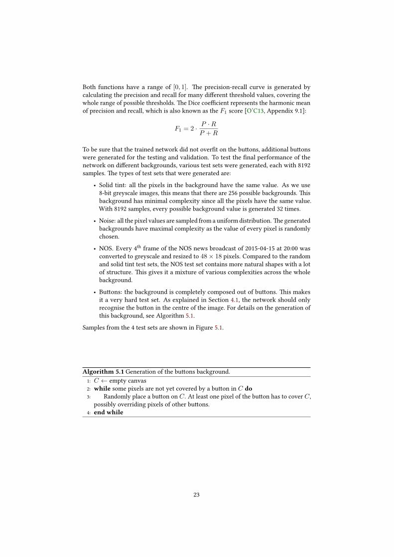
• Bu�ons: the background is completely composed out of bu�ons. �is makesit a very hard test set. As explained in Section 4.1, the network should onlyrecognise the bu�on in the centre of the image. For details on the generation ofthis background, see Algorithm 5.1.

Samples from the 4 test sets are shown in Figure 5.1.

Algorithm 5.1 Generation of the bu�ons background.1: C ← empty canvas2: while some pixels are not yet covered by a bu�on in C do3: Randomly place a bu�on on C . At least one pixel of the bu�on has to cover C ,

possibly overriding pixels of other bu�ons.4: end while

23

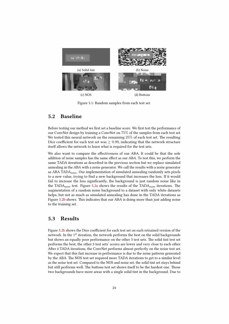
(a) Solid tint (b) Noise

(c) NOS (d) Bu�ons

Figure 5.1: Random samples from each test set.

5.2 Baseline

Before testing our method we �rst set a baseline score. We �rst test the performance ofour ConvNet design by training a ConvNet on 75% of the samples from each test set.We tested this neural network on the remaining 25% of each test set. �e resultingDice coe�cient for each test set was ≥ 0.99, indicating that the network structureitself allows the network to learn what is required for the test sets.

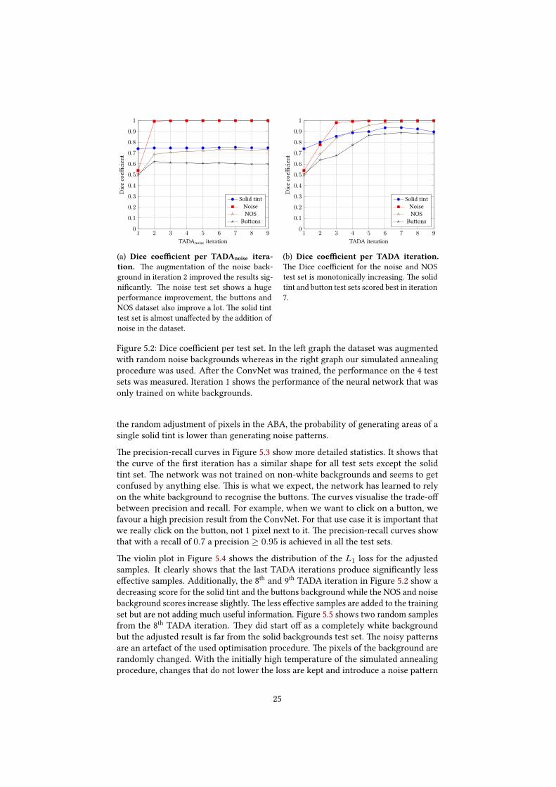
We also want to compare the e�ectiveness of our ABA. It could be that the soleaddition of noise samples has the same e�ect as our ABA. To test this, we perform thesame TADA iterations as described in the previous section but we replace simulatedannealing in the ABA with a noise generator. We call the results with a noise generatoras ABA TADAnoise. Our implementation of simulated annealing randomly sets pixelsto a new value, trying to �nd a new background that increases the loss. If it wouldfail to increase the loss signi�cantly, the background is just random noise like inthe TADAnoise test. Figure 5.2a shows the results of the TADAnoise iterations. �eaugmentation of a random noise background to a dataset with only white datasetshelps, but not as much as simulated annealing has done in the TADA iterations asFigure 5.2b shows. �is indicates that our ABA is doing more than just adding noiseto the training set.

5.3 Results

Figure 5.2b shows the Dice coe�cient for each test set on each retrained version of thenetwork. In the 1st iteration, the network performs the best on the solid backgroundsbut shows an equally poor performance on the other 3 test sets. �e solid tint test setperforms the best, the other 3 test sets’ scores are lower and very close to each other.A�er 4 TADA iterations, the ConvNet performs almost perfectly on the noise test set.We expect that this fast increase in performance is due to the noise pa�erns generatedby the ABA. �e NOS test set required more TADA iterations to get to a similar levelas the noise test set. Compared to the NOS and noise set, the solid tint set stays behindbut still performs well. �e bu�ons test set shows itself to be the hardest one. �osetwo backgrounds have more areas with a single solid tint in the background. Due to

24

1 2 3 4 5 6 7 8 90

0.1

0.2

0.3

0.4

0.5

0.6

0.7

0.8

0.9

1

TADAnoise iteration

Dicecoe�

cient

Solid tintNoiseNOS

Bu�ons

(a) Dice coe�cient per TADAnoise itera-tion. �e augmentation of the noise back-ground in iteration 2 improved the results sig-ni�cantly. �e noise test set shows a hugeperformance improvement, the bu�ons andNOS dataset also improve a lot. �e solid tinttest set is almost una�ected by the addition ofnoise in the dataset.

1 2 3 4 5 6 7 8 90

0.1

0.2

0.3

0.4

0.5

0.6

0.7

0.8

0.9

1

TADA iteration

Dicecoe�

cient

Solid tintNoiseNOS

Bu�ons

(b) Dice coe�cient per TADA iteration.�e Dice coe�cient for the noise and NOStest set is monotonically increasing. �e solidtint and bu�on test sets scored best in iteration7.

Figure 5.2: Dice coe�cient per test set. In the le� graph the dataset was augmentedwith random noise backgrounds whereas in the right graph our simulated annealingprocedure was used. A�er the ConvNet was trained, the performance on the 4 testsets was measured. Iteration 1 shows the performance of the neural network that wasonly trained on white backgrounds.

the random adjustment of pixels in the ABA, the probability of generating areas of asingle solid tint is lower than generating noise pa�erns.

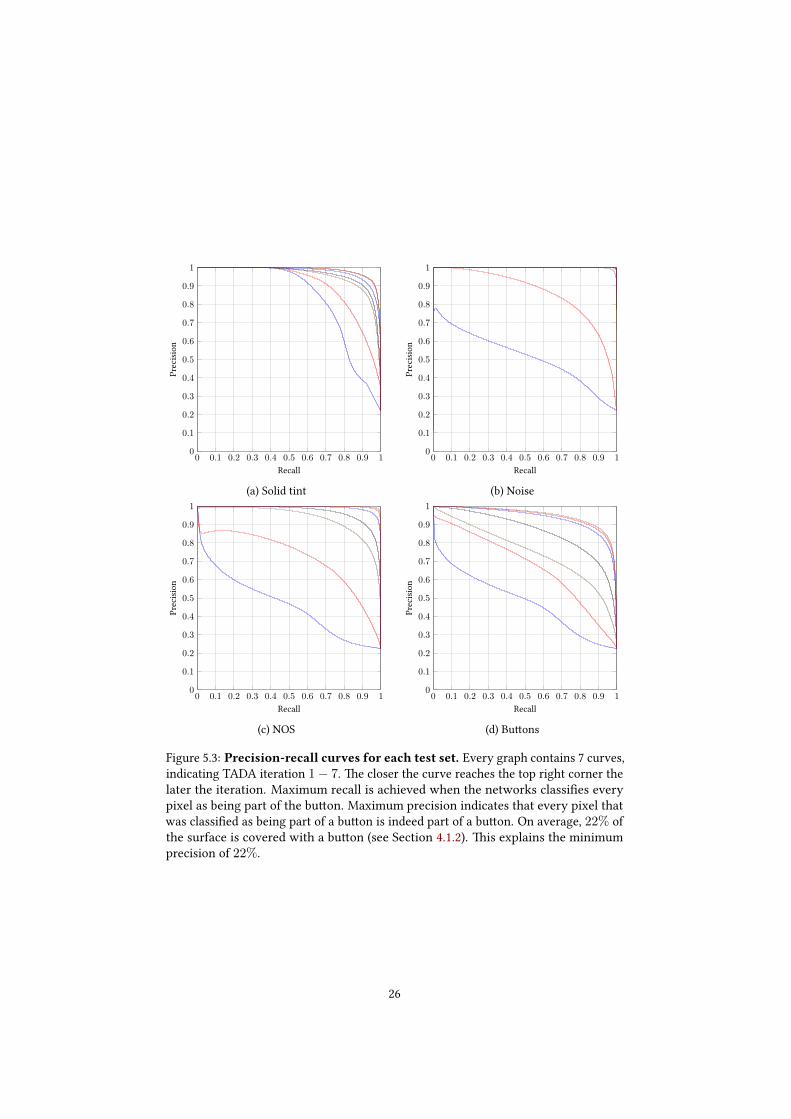
�e precision-recall curves in Figure 5.3 show more detailed statistics. It shows thatthe curve of the �rst iteration has a similar shape for all test sets except the solidtint set. �e network was not trained on non-white backgrounds and seems to getconfused by anything else. �is is what we expect, the network has learned to relyon the white background to recognise the bu�ons. �e curves visualise the trade-o�between precision and recall. For example, when we want to click on a bu�on, wefavour a high precision result from the ConvNet. For that use case it is important thatwe really click on the bu�on, not 1 pixel next to it. �e precision-recall curves showthat with a recall of 0.7 a precision ≥ 0.95 is achieved in all the test sets.

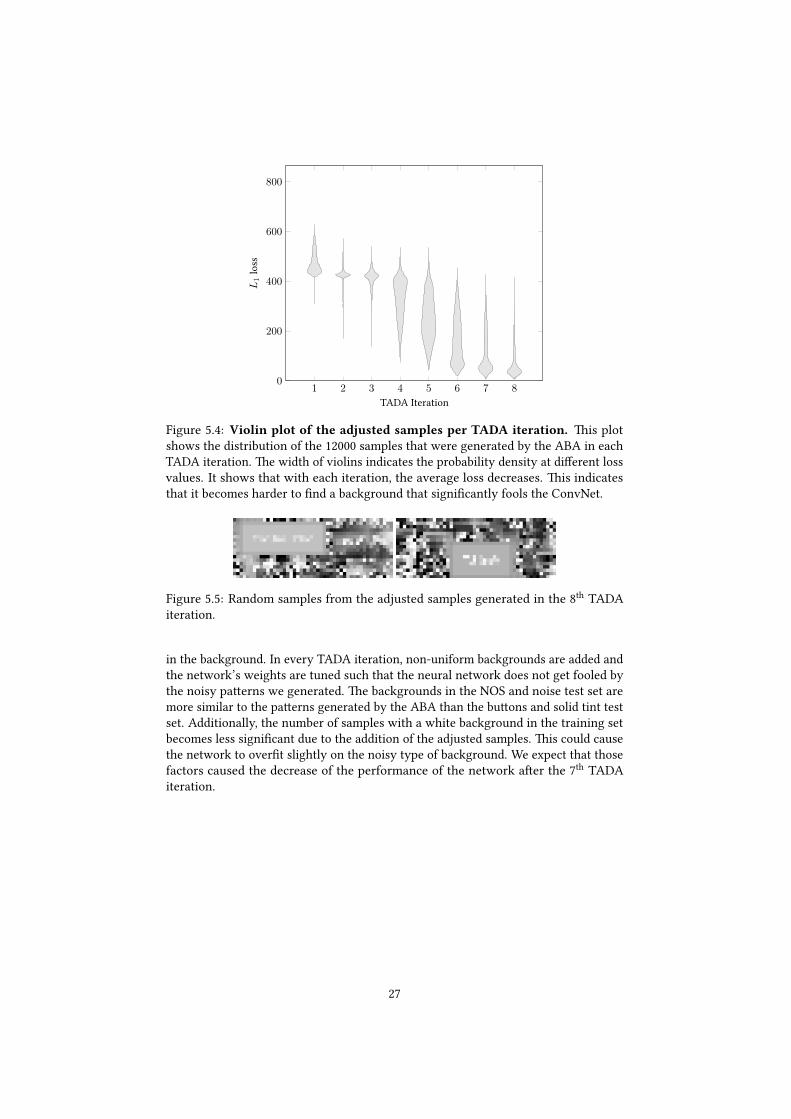
�e violin plot in Figure 5.4 shows the distribution of the L1 loss for the adjustedsamples. It clearly shows that the last TADA iterations produce signi�cantly lesse�ective samples. Additionally, the 8th and 9th TADA iteration in Figure 5.2 show adecreasing score for the solid tint and the bu�ons background while the NOS and noisebackground scores increase slightly. �e less e�ective samples are added to the trainingset but are not adding much useful information. Figure 5.5 shows two random samplesfrom the 8th TADA iteration. �ey did start o� as a completely white backgroundbut the adjusted result is far from the solid backgrounds test set. �e noisy pa�ernsare an artefact of the used optimisation procedure. �e pixels of the background arerandomly changed. With the initially high temperature of the simulated annealingprocedure, changes that do not lower the loss are kept and introduce a noise pa�ern

25

0 0.1 0.2 0.3 0.4 0.5 0.6 0.7 0.8 0.9 10

0.1

0.2

0.3

0.4

0.5

0.6

0.7

0.8

0.9

1

Recall

Precision

(a) Solid tint

0 0.1 0.2 0.3 0.4 0.5 0.6 0.7 0.8 0.9 10

0.1

0.2

0.3

0.4

0.5

0.6

0.7

0.8

0.9

1

Recall

Precision

(b) Noise

0 0.1 0.2 0.3 0.4 0.5 0.6 0.7 0.8 0.9 10

0.1

0.2

0.3

0.4

0.5

0.6

0.7

0.8

0.9

1

Recall

Precision

(c) NOS

0 0.1 0.2 0.3 0.4 0.5 0.6 0.7 0.8 0.9 10

0.1

0.2

0.3

0.4

0.5

0.6

0.7

0.8

0.9

1

Recall

Precision

(d) Bu�ons

Figure 5.3: Precision-recall curves for each test set. Every graph contains 7 curves,indicating TADA iteration 1− 7. �e closer the curve reaches the top right corner thelater the iteration. Maximum recall is achieved when the networks classi�es everypixel as being part of the bu�on. Maximum precision indicates that every pixel thatwas classi�ed as being part of a bu�on is indeed part of a bu�on. On average, 22% ofthe surface is covered with a bu�on (see Section 4.1.2). �is explains the minimumprecision of 22%.

26

1 2 3 4 5 6 7 80

200

400

600

800

TADA Iteration

L1loss

Figure 5.4: Violin plot of the adjusted samples per TADA iteration. �is plotshows the distribution of the 12000 samples that were generated by the ABA in eachTADA iteration. �e width of violins indicates the probability density at di�erent lossvalues. It shows that with each iteration, the average loss decreases. �is indicatesthat it becomes harder to �nd a background that signi�cantly fools the ConvNet.

Figure 5.5: Random samples from the adjusted samples generated in the 8th TADAiteration.

in the background. In every TADA iteration, non-uniform backgrounds are added andthe network’s weights are tuned such that the neural network does not get fooled bythe noisy pa�erns we generated. �e backgrounds in the NOS and noise test set aremore similar to the pa�erns generated by the ABA than the bu�ons and solid tint testset. Additionally, the number of samples with a white background in the training setbecomes less signi�cant due to the addition of the adjusted samples. �is could causethe network to over�t slightly on the noisy type of background. We expect that thosefactors caused the decrease of the performance of the network a�er the 7th TADAiteration.

27

5.4 Conclusion

We found that using our adversarial background augmentation procedure to train aConvNet improves the generalisation performance of that ConvNet. In this thesis,we trained a ConvNet on a training set with a bu�on in front of a completely whitebackground. �is network was retrained on adversarial backgrounds. �e philosophybehind our approach is that adversarial backgrounds exploit weaknesses of the net-work’s way of localising bu�ons. Retraining with adversarial backgrounds gives thenetwork the opportunity to correct those weaknesses.

We precisely de�ned a model that captures how the bu�ons we want to localise maylook. Based on that model we sampled as many bu�ons as we needed for training.�is allows the network to learn to recognise the shared properties of the bu�onsto localise. �e background around the bu�on is also important. A network that istrained on a background that is too simple will get confused when it sees other typesof backgrounds. It becomes dependent on this background instead of the features ofthe bu�on itself. Instead of creating a representative model for the backgrounds thatthe network could ever encounter a�er training, we found that we could generateadversarial backgrounds. �is eliminates the need to manually design a model for thebackground around the bu�on.

We initially trained a ConvNet on bu�ons in front of a completely white background.Via TADA iterations we improved this network by retraining it on adversarial back-grounds. We found that applying multiple TADA iterations helped to improve thenetwork’s performance signi�cantly. �e �nal ConvNet generalised much be�er tounseen backgrounds. Simply using completely white and noise backgrounds to trainthe ConvNet yielded a Dice coe�cient of 0.74 on the NOS test set, our method booststhis score by 34% to 0.99. �is is a close to perfect score.

Our method of adversarial background augmentation opens up ways to easily trainnew object localisers. It has allowed us to develop a bu�on localiser without having todesign a model of the background around it. Our method simply requires su�cientsamples of the object to recognise and a ConvNet structure with a correspondingtraining procedure. �ough we only tested our method on bu�ons, our method is notspeci�cally designed for bu�ons. We expect that our method can be applied to otherobjects as well. �e ConvNet learns from the data and our adversarial backgroundsare adapted to the trained ConvNet.

5.5 Future work

Our implementation of simulated annealing sets a random pixel of the background toa new random value. �is is an ine�cient way to generate adversarial backgrounds.In every TADA iteration, it takes approximately 18 hours to generate the optimisedsamples. Although this time can be shortened by tuning the annealing scheduleand simplifying the neural network structure even more, we could try to infer theadversarial samples directly from the network itself via gradient ascent [EBCV09,SVZ14]. Since the adversarial samples are inferred from the network itself, we expectthose adversarial samples are be�er and faster to generate. A more e�cient ABA could

28

also make using higher input resolutions more practical. �e higher the resolution,the more pixels that can be altered and thus the more e�ort required.

Every sample in our training set always contained a bu�on. �e resulting neuralnetwork cannot cope with samples that do not contain a bu�on at all. In Section 4.1,we explained that the ABA could start drawing actual bu�ons in the background whilewe tell the network that there is no bu�on at that location. �e probability that thesimulated annealing algorithm will generate a bu�on that conforms to our model isvery low. Even if it would occur, we expect that the majority of the samples will stillsteer the network in the right direction. On the other hand, it could cause the networkto be overly conservative in its predictions. We also did not consider the case withmore than one bu�on in the input. We had the requirement that the bu�on was partof the centre of the input (see Section 4.1). To detect bu�ons in a large image, wewould need to apply this network at many positions of that image. Every bu�on ofthe large image has to be part of the centre of the neural network in order for it tobe detected. So when sliding the input of the neural network over the large image,the stride is dependent on the minimum dimensions of the bu�ons. By dropping thisrequirement, the whole input of the neural network can be used to detect bu�ons,saving computation time. It also opens ways to localise multiple bu�ons at once.

Our method uses a binary output mask to give a pixel-wise annotation of the location ofthe bu�on. �is level of detail might not be needed. In our case, a 4D vector with loca-tion of the bu�on could also be su�cient. �e 4D vector can represent the coordinatesof the centre, the width and height of the bu�on (e.g. [SZ15]). Alternatively, the 4Dcoordinate could represent the coordinates of the bounding box (e.g. [WZL+14]). �eMultiBox method [ESTA14, SREA14, HZRS15] uses a 4D vector system and supportslocating a dynamic number of objects via a ConvNet.

We only tested with a square bu�on with limited variety. We would like to knowhow our method would perform on more complex objects to recognise. Our object torecognise could be modelled as a 3D model. �e 3D model gives the required binarymask of its location. Our method can generate the backgrounds around it. Insteadof localisation, this might also help training classi�ers that assign a category to animage. In future work we could test our method on existing datasets to compare theperformance with the state of the art.

In every TADA iteration, we add more samples to the dataset. �e more TADAiterations we do, the lower the impact of the new samples. In every iteration it alsobecomes harder to generate samples that signi�cantly fool the network. Since theimpact of the new samples is also reduced, the learning slows down. Environmentswhere more TADA iterations are required might bene�t from a di�erent augmentationscheme. A di�erent augmentation scheme that drops older samples or favours newersamples during training might speed up learning.

29

Bibliography

[BBB+10] James Bergstra, Olivier Breuleux, Frederic Bastien, Pascal Lamblin,Razvan Pascanu, Guillaume Desjardins, Joseph Turian, David Warde-Farley, and Yoshua Bengio. �eano: a CPU and GPU math expressioncompiler. In Proceedings of the Python for Scienti�c Computing Con-ference (SciPy), 2010. URL: http://www-etud.iro.umontreal.ca/~wardefar/publications/theano_scipy2010.pdf. 7

[BHC15] Vijay Badrinarayanan, Ankur Handa, and Roberto Cipolla. Segnet: Adeep convolutional encoder-decoder architecture for robust semanticpixel-wise labelling. CoRR, abs/1505.07293, 2015. URL: http://arxiv.org/abs/1505.07293. 7

[Bis95] C.M. Bishop. Neural Networks for Pa�ern Recognition. Clarendon Press,1995. 20

[CKF11] Ronan Collobert, Koray Kavukcuoglu, and Clement Farabet. Torch7: Amatlab-like environment for machine learning. In BigLearn, NIPS Work-shop, 2011. URL: http://infoscience.epfl.ch/record/192376/files/Collobert_NIPSWORKSHOP_2011.pdf. 7

[CM00] D. Connolly and L. Masinter. RFC2854: �e ’text/html’ Media Type, 2000.URL: https://tools.ietf.org/html/rfc2854. 15

[CMS12] Dan Ciresan, Ueli Meier, and Jurgen Schmidhuber. Multi-column deepneural networks for image classi�cation. In Computer Vision and Pa�ernRecognition (CVPR), 2012 IEEE Conference on, 2012. URL: http://arxiv.org/abs/1202.2745. 7, 8

[Cor15] Nvidia Corporation. CUDA C Programming Guide, 2015.URL: http://docs.nvidia.com/cuda/cuda-c-programming-

guide/index.html. 7

[CW08] Ronan Collobert and Jason Weston. A uni�ed architecture for naturallanguage processing: Deep neural networks with multitask learning. InInternational Conference on Machine Learning, ICML, 2008. URL: http://ronan.collobert.com/pub/matos/2008_nlp_icml.pdf. 1

[DB15] Alexey Dosovitskiy and �omas Brox. Inverting convolutional networkswith convolutional networks. CoRR, 2015. URL: http://arxiv.org/abs/1506.02753. 17

30

[DF10] Morgan Dixon and James Fogarty. Prefab: Implementing Advanced Be-haviors Using Pixel-Based Reverse Engineering of Interface Structure. InProceedings of the SIGCHI Conference on Human Factors in Computing Sys-tems, pages 1525–1534, 2010. URL: https://homes.cs.washington.edu/~jfogarty/publications/chi2010-prefab.pdf. 6

[Dic45] Lee R. Dice. Measures of the Amount of Ecologic Association BetweenSpecies. Ecology, 26(3):297–302, 1945. URL: http://www.jstor.org/stable/1932409. 22

[DYDA12] George E. Dahl, Dong Yu, Li Deng, and Alex Acero. Context-DependentPre-Trained Deep Neural Networks for Large-Vocabulary Speech Recog-nition. IEEE Transactions on Audio, Speech and Language Processing,20(1):30–42, 2012. URL: http://research.microsoft.com/apps/pubs/default.aspx?id=144412. 1

[EBCV09] Dumitru Erhan, Yoshua Bengio, Aaron Courville, and Pascal Vin-cent. Visualizing higher-layer features of a deep network. Dept.IRO, Universite de Montreal, Tech. Rep, 4323, 2009. URL: http:

//igva2012.wikispaces.asu.edu/file/view/Erhan+2009+

Visualizing+higher+layer+features+of+a+deep+network.pdf.28

[ESTA14] Dumitru Erhan, Christian Szegedy, Alexander Toshev, and DragomirAnguelov. Scalable Object Detection using Deep Neural Networks. InComputer Vision and Pa�ern Recognition (CVPR), 2014 IEEE Conferenceon, pages 2155–2162. IEEE, 2014. URL: http://arxiv.org/abs/1312.2249. 6, 8, 29

[Ete11] Elika J. Etemad. Cascading Style Sheets (CSS) Snapshot 2010, 2011. URL:http://www.w3.org/TR/2011/NOTE-css-2010-20110512/. 15

[EvW+09] Mark Everingham, Luc van Gool, Christopher K. I. Williams, JohnWinn, and Andrew Zisserman. �e Pascal Visual Object Classes(VOC) Challenge. International Journal of Computer Vision, 88(2),September 2009. URL: http://research.microsoft.com/apps/

pubs/default.aspx?id=102944. 6

[Fau06] Kjell Magne Fauske. Example: Neural network, 2006. URL: http://www.texample.net/tikz/examples/neural-network/. 11

[FCNL12] Clement Farabet, Camille Couprie, Laurent Najman, and Yann LeCun.Scene Parsing with Multiscale Feature Learning, Purity Trees, and Op-timal Covers. In Proc. International Conference on Machine learning(ICML’12), 2012. URL: http://arxiv.org/abs/1202.2160. 7

[FGMR10] Pedro F. Felzenszwalb, Ross B. Girshick, David McAllester, and DevaRamanan. Object Detection with Discriminatively Trained Part BasedModels. Pa�ern Analysis and Machine Intelligence, IEEE Transactions on,32(9):1627–1645, 2010. URL: http://cs.brown.edu/~pff/papers/lsvm-pami.pdf. 6

[GDDM14] Ross Girshick, Je� Donahue, Trevor Darrell, and Jitendra Malik. Rich fea-ture hierarchies for accurate object detection and semantic segmentation.In Computer Vision and Pa�ern Recognition (CVPR), 2014 IEEE Conference

31

on, pages 2–9. IEEE, 2014. URL: http://arxiv.org/abs/1311.2524.1, 8

[GR15] Shixiang Gu and Luca Rigazio. Towards Deep Neural Network Ar-chitectures Robust to Adversarial Examples. CoRR, 2015. URL: http://arxiv.org/abs/1412.5068. 8, 9

[GSS15] Ian J Goodfellow, Jonathon Shlens, and Christian Szegedy. Explainingand Harnessing Adversarial Examples. CoRR, 2015. URL: http://arxiv.org/abs/1412.6572. 8, 9

[GWFL+13] Ian J. Goodfellow, David Warde-Farley, Pascal Lamblin, Vincent Du-moulin, Mehdi Mirza, Razvan Pascanu, James Bergstra, Frederic Bastien,and Yoshua Bengio. Pylearn2: a machine learning research library. 2013.URL: http://arxiv.org/abs/1308.4214. 7

[GWS] Kevin Gibbs, Terry Winograd, and Neil Sco�. Lens: A System for Vi-sual Interpretation of Graphical User Interfaces. URL: https://cs.stanford.edu/~kgibbs/lens.pdf. 6

[HAGM14] Bharath Hariharan, Pablo Arbelaez, Ross Girshick, and Jitendra Malik. Si-multaneous Detection and Segmentation. In European Conference on Com-puter Vision (ECCV), 2014. URL: http://www.eecs.berkeley.edu/Research/Projects/CS/vision/papers/BharathECCV2014.pdf.7

[Hay99] Simon S. Haykin. Neural Networks: A Comprehensive Foundation. PrenticeHall, 1999. 10, 17

[Hin14] Geo�rey Hinton. Dropout : A simple way to prevent neural net-works from over��ing. �e Journal of Machine Learning Research,15(1):1929–1958, 2014. URL: http://jmlr.org/papers/volume15/srivastava14a/srivastava14a.pdf. 7

[How13] Andrew G. Howard. Some Improvements on Deep Convolutional NeuralNetwork Based Image Classi�cation. CoRR, 2013. URL: http://arxiv.org/abs/1312.5402. 7

[HZRS15] Kaiming He, Xiangyu Zhang, Shaoqing Ren, and Jian Sun. DelvingDeep into Recti�ers: Surpassing Human-Level Performance on ImageNetClassi�cation. CoRR, 2015. URL: http://arxiv.org/abs/1502.01852.1, 16, 29

[JSD+14] Yangqing Jia, Evan Shelhamer, Je� Donahue, Sergey Karayev, JonathanLong, Ross B. Girshick, Sergio Guadarrama, and Trevor Darrell. Ca�e:Convolutional architecture for fast feature embedding. CoRR, 2014. URL:http://arxiv.org/abs/1408.5093. 7, 16

[Kar15] Andrej Karpathy. Convolutional Neural Networks, 2015. URL:https://github.com/cs231n/cs231n.github.io/blob/

2e3b53f36d524b3c95c1e731c97a7e0c391aa78d/convolutional-

networks.md. 12

[KGV83] S. Kirkpatrick, C. D. Gela�, and M. P. Vecchi. Optimization by simulatedannealing. Science, 220(4598):671–680, 1983. URL: http://www.jstor.org/stable/1690046. 12

32

[KHK08] Takuya Kobayashi, Akinori Hidaka, and Takio Kurita. Selection of his-tograms of oriented gradients features for pedestrian detection. In NeuralInformation Processing, volume 4985 of Lecture Notes in Computer Science,pages 598–607. Springer Berlin Heidelberg, 2008. URL: http://link.springer.com/chapter/10.1007/978-3-540-69162-4_62. 6

[KSH12] Alex Krizhevsky, Ilya Sutskever, and Geo�rey Hinton. In Advancesin Neural Information Processing Systems 25, pages 1097–1105. CurranAssociates, Inc., 2012. URL: http://papers.nips.cc/paper/4824-imagenet-classification-w. 1, 5, 6, 7, 8, 16, 17, 18, 19

[LBBH98] Yann LeCun, Leon Bo�ou, Yoshua Bengio, and Patrick Ha�ner. Gradient-based learning applied to document recognition. Proceedings of the IEEE,86(11):2278–2324, November 1998. URL: http://yann.lecun.com/exdb/publis/pdf/lecun-98.pdf. 7

[LBH15] Yann LeCun, Yoshua Bengio, and Geo�rey Hinton. Deep learning. Nature,521(7553):436–444, 2015. URL: http://go.nature.com/7cjbaa. 7, 10

[LCY13] Min Lin, Qiang Chen, and Shuicheng Yan. Network In Network. CoRR,2013. URL: http://arxiv.org/abs/1312.4400. 7, 8

[Low04] David G Lowe. Distinctive Image Features from Scale-Invariant Keypoints.International journal of computer vision, 60(2):91–110, 2004. URL: http://www.cs.ubc.ca/~lowe/papers/ijcv04.pdf. 6

[MP43] Warren S. McCulloch and Walter Pi�s. A logical calculus of the ideasimmanent in nervous activity. �e bulletin of mathematical biophysics,5(4):115–133, 1943. URL: http://link.springer.com/article/10.1007/BF02478259. 1

[NYC15] Anh Nguyen, Jason Yosinski, and Je� Clune. Deep neural networks areeasily fooled: High con�dence predictions for unrecognizable images. InComputer Vision and Pa�ern Recognition (CVPR), 2015 IEEE Conference on.IEEE, 2015. URL: http://www.evolvingai.org/fooling. 7, 8, 9

[OBLS14] Maxime Oquab, Leon Bo�ou, Ivan Laptev, and Josef Sivic. Learningand Transferring Mid-Level Image Representations using ConvolutionalNeural Networks. In Computer Vision and Pa�ern Recognition (CVPR),2014 IEEE Conference on, 2014. URL: http://www.di.ens.fr/willow/research/cnn/. 6, 8

[OBLS15] Maxime Oquab, Leon Bo�ou, Ivan Laptev, and Josef Sivic. Is objectlocalization for free? – Weakly supervised object recognition withconvolutional neural networks. In Proceedings of the IEEE Confer-ence on Computer Vision and Pa�ern Recognition, 2015. URL: http://www.di.ens.fr/willow/research/weakcnn/. 6, 8

[O’C13] Brendan O’Connor. Learning Frames from Text with an UnsupervisedLatent Variable Model. CoRR, 2013. URL: http://arxiv.org/abs/1307.7382. 23

[OLZ+14] Wanli Ouyang, Ping Luo, Xingyu Zeng, Shi Qiu, Yonglong Tian, Hong-sheng Li, Shuo Yang, Zhe Wang, Yuanjun Xiong, Chen Qian, ZhenyaoZhu, Ruohui Wang, Chen-Change Loy, Xiaogang Wang, and Xiaoou

33

Tang. DeepID-Net: multi-stage and deformable deep convolutional neu-ral networks for object detection. 2014. URL: http://arxiv.org/abs/1409.3505. 8

[RDS+15] Olga Russakovsky, Jia Deng, Hao Su, Jonathan Krause, Sanjeev Satheesh,Sean Ma, Zhiheng Huang, Andrej Karpathy, Aditya Khosla, MichaelBernstein, Alexander Berg C., and Fei-Fei Li. ImageNet Large ScaleVisual Recognition Challenge. International Journal of Computer Vision(IJCV), 2015. URL: http://arxiv.org/abs/1409.0575. 6, 7

[Ros58] Frank Rosenbla�. �e perceptron: a probabilistic model for informationstorage and organization in the brain. Psychological Review, 65(6):386–408,1958. 1

[Sch15] Jurgen Schmidhuber. Deep Learning in Neural Networks: An Overview.Neural Networks, 61:85–117, 2015. URL: http://arxiv.org/abs/1404.7828. 10

[SD15] Evan Shelhamer and Je� Donahue. Ca�e — Solver / Model opti-mization, 2015. URL: https://github.com/BVLC/caffe/blob/

648aed72acf1c506009ddb33d8cace40b75e176e/docs/tutorial/

solver.md. 19

[SDK15] Evan Shelhamer, Je� Donahue, and Sergey Karayev. BVLC’s AlexNetmodel, 2015. URL: https://github.com/BVLC/caffe/tree/

e6c80dac40d4bb13390b56bc18294e6e91b00436/models/bvlc_

alexnet. 16, 17, 18, 19

[SEZ+14] Pierre Sermanet, David Eigen, Xiang Zhang, Michael Mathieu, RobFergus, and Yann LeCun. OverFeat : Integrated Recognition, Lo-calization and Detection using Convolutional Networks. In Inter-national Conference on Learning Representations (ICLR 2014). CBLS,2014. URL: http://openreview.net/document/cb1bf585-d8ae-4de7-aa0c-f47cdc763d8d. 1, 6, 8

[SLJ+15] Christian Szegedy, Wei Liu, Yangqing Jia, Pierre Sermanet, Sco� Reed,Dragomir Anguelov, Dumitru Erhan, Vincent Vanhoucke, and AndrewRabinovich. Going deeper with convolutions. In CVPR 2015, 2015. URL:http://arxiv.org/abs/1409.4842. 8

[SQLG15] Hao Su, Charles R. Qi, Yangyan Li, and Leonidas J. Guibas. Renderfor CNN: Viewpoint Estimation in Images Using CNNs Trained withRendered 3D Model Views. CoRR, 2015. URL: http://arxiv.org/abs/1505.05641. 8, 9

[SREA14] Christian Szegedy, Sco� Reed, Dumitru Erhan, and Dragomir Anguelov.Scalable, High-�ality Object Detection. CoRR, 2014. URL: http://arxiv.org/abs/1412.1441. 8, 29

[SS14] Baochen Sun and Kate Saenko. From Virtual to Reality: Fast Adaptationof Virtual Object Detectors to Real Domains. In Proceedings of the BritishMachine Vision Conference. BMVA Press, 2014. URL: http://www.bmva.org/bmvc/2014/papers/paper062/index.html. 8, 9

34

[STE13] Christian Szegedy, Alexander Toshev, and Dumitru Erhan. Deep neu-ral networks for object detection. In Advances in Neural Informa-tion Processing Systems 26, pages 2553–2561. Curran Associates, Inc.,2013. URL: http://papers.nips.cc/paper/5207-deep-neural-networks-for-object-detection.pdf. 1, 6, 8, 16, 17

[SVZ14] Karen Simonyan, Andrea Vedaldi, and Andrew Zisserman. Deep InsideConvolutional Networks: Visualising Image Classi�cation Models andSaliency Maps. In Workshop at International Conference on LearningRepresentations, 2014. URL: http://arxiv.org/abs/1312.6034. 6, 8,28

[SZ15] Karen Simonyan and Andrew Zisserman. Very Deep ConvolutionalNetworks for Large-Scale Image Recognition. In International Conferenceon Learning Representations, 2015. URL: http://arxiv.org/abs/1409.1556. 1, 7, 8, 16, 17, 29

[SZS+14] Christian Szegedy, Wojciech Zaremba, Ilya Sutskever, Joan Bruna, Du-mitru Erhan, Ian Goodfellow, and Rob Fergus. Intriguing properties ofneural networks. In International Conference on Learning Representations,2014. URL: http://arxiv.org/abs/1312.6199. 8

[TYRW14] Yaniv Taigman, Ming Yang, Marc’Aurelio Ranzato, and Lior Wolf. Deep-Face: Closing the Gap to Human-Level Performance in Face Veri�ca-tion. In Computer Vision and Pa�ern Recognition (CVPR), 2014 IEEE Con-ference on, 2014. URL: http://www.cs.tau.ac.il/~wolf/papers/deepface_11_01_2013.pdf. 7

[Van79] C. J. Van Rijsbergen. Information Retrieval. 1979. URL: http://www.dcs.gla.ac.uk/Keith/Preface.html. 22

[WZL+14] Xiaolong Wang, Liliang Zhang, Liang Lin, Zhujin Liang, and WangmengZuo. Deep Joint Task Learning for Generic Object Extraction. In Advancesin Neural Information Processing Systems 27, pages 523–531. Curran Asso-ciates, Inc., 2014. URL: http://papers.nips.cc/paper/5547-deep-joint-task-learning-for-generic-object-extraction.pdf.6, 8, 29

[ZDGD14] Ning Zhang, Je� Donahue, Ross Girshick, and Trevor Darrell. Part-based R-CNNs for �ne-grained category detection. In Proceedings ofthe European Conference on Computer Vision (ECCV), 2014. URL: http://arxiv.org/pdf/1407.3867.pdf. 8

[ZF14] Ma�hew D Zeiler and Rob Fergus. Visualizing and Understanding Con-volutional Networks. In Computer Vision–ECCV 2014, volume 8689 ofLecture Notes in Computer Science, pages 818–833. Springer InternationalPublishing, 2014. URL: http://arxiv.org/abs/1311.2901. 5, 8, 16,17

[ZKL+14] Bolei Zhou, Aditya Khosla, Agata Lapedriza, Aude Olivia, and AntonioTorralba. Object Detectors Emerge in Deep Scene CNNs. CoRR, 2014.URL: http://arxiv.org/abs/1412.6856. 8

35

Acronyms

ABA Adversarial Background Adjuster. 5, 14, 15, 19, 24, 25, 27–29

ANN Arti�cial Neural Network. 1, 2

BVLC Berkeley Vision and Learning Center. 16–19

ConvNet Convolutional Neural Network. 1, 2, 4–8, 12, 14, 15, 19, 22, 24, 25, 27–29

CPU Central Processing Unit. 7

CSS Cascading Style Sheet. 15, 16

DNN Deep Neural Network. 2, 8, 10, 11

DPM Deformable Parts Model. 6

GPGPU General Purpose computation on GPUs. 7

GPU Graphics Processing Unit. 1, 7, 17, 36

HOG Histograms of Oriented Gradients. 6

HTML HyperText Markup Language. 15

LRN Local Response Normalisation. 18

NOS Nederlandse Omroep Stichting, English: Dutch Broadcast Foundation. 15, 23, 27,28

NTA Nedap Testing Automation. 3

R-CNN Regions with CNN features. 8

SGD Stochastic Gradient Descent. 10

SIFT Scale Invariant Feature Transform. 6

SIMD Single Instruction Multiple Data. 7

TADA Train ADjust Augment. 5, 14, 17, 19–22, 24–29

36