Workshop track - ICLR 2017

ADVERSARIAL EXAMPLES IN THE PHYSICAL WORLD

Alexey KurakinGoogle Brainkurakin@google.com

Ian J. GoodfellowOpenAIian@openai.com

Samy BengioGoogle Brainbengio@google.com

ABSTRACT

Most existing machine learning classifiers are highly vulnerable to adversarialexamples. An adversarial example is a sample of input data which has been mod-ified very slightly in a way that is intended to cause a machine learning classifierto misclassify it. In many cases, these modifications can be so subtle that a humanobserver does not even notice the modification at all, yet the classifier still makesa mistake. Adversarial examples pose security concerns because they could beused to perform an attack on machine learning systems, even if the adversary hasno access to the underlying model. Up to now, all previous work has assumed athreat model in which the adversary can feed data directly into the machine learn-ing classifier. This is not always the case for systems operating in the physicalworld, for example those which are using signals from cameras and other sensorsas input. This paper shows that even in such physical world scenarios, machinelearning systems are vulnerable to adversarial examples. We demonstrate this byfeeding adversarial images obtained from a cell-phone camera to an ImageNet In-ception classifier and measuring the classification accuracy of the system. We findthat a large fraction of adversarial examples are classified incorrectly even whenperceived through the camera.

1 INTRODUCTION

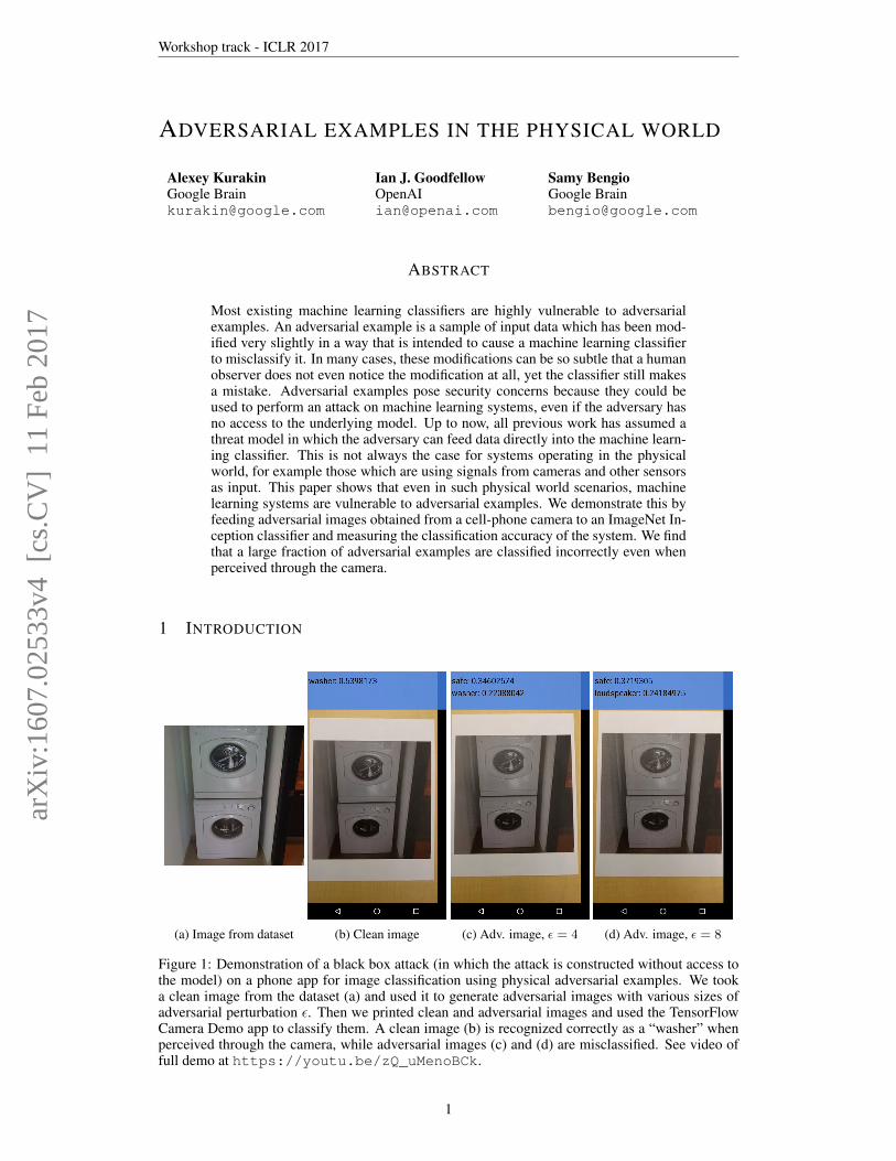
(a) Image from dataset (b) Clean image (c) Adv. image, ε = 4 (d) Adv. image, ε = 8

Figure 1: Demonstration of a black box attack (in which the attack is constructed without access tothe model) on a phone app for image classification using physical adversarial examples. We tooka clean image from the dataset (a) and used it to generate adversarial images with various sizes ofadversarial perturbation ε. Then we printed clean and adversarial images and used the TensorFlowCamera Demo app to classify them. A clean image (b) is recognized correctly as a “washer” whenperceived through the camera, while adversarial images (c) and (d) are misclassified. See video offull demo at https://youtu.be/zQ_uMenoBCk.

1

arX

iv:1

607.

0253

3v4

[cs

.CV

] 1

1 Fe

b 20

17

Workshop track - ICLR 2017

Recent advances in machine learning and deep neural networks enabled researchers to solve multipleimportant practical problems like image, video, text classification and others (Krizhevsky et al.,2012; Hinton et al., 2012; Bahdanau et al., 2015).

However, machine learning models are often vulnerable to adversarial manipulation of their input in-tended to cause incorrect classification (Dalvi et al., 2004). In particular, neural networks and manyother categories of machine learning models are highly vulnerable to attacks based on small modifi-cations of the input to the model at test time (Biggio et al., 2013; Szegedy et al., 2014; Goodfellowet al., 2014; Papernot et al., 2016b).

The problem can be summarized as follows. Let’s say there is a machine learning system M andinput sample C which we call a clean example. Let’s assume that sample C is correctly classified bythe machine learning system, i.e. M(C) = ytrue. It’s possible to construct an adversarial exampleA which is perceptually indistinguishable from C but is classified incorrectly, i.e. M(A) 6= ytrue.These adversarial examples are misclassified far more often than examples that have been perturbedby noise, even if the magnitude of the noise is much larger than the magnitude of the adversarialperturbation (Szegedy et al., 2014).

Adversarial examples pose potential security threats for practical machine learning applications.In particular, Szegedy et al. (2014) showed that an adversarial example that was designed to bemisclassified by a model M1 is often also misclassified by a model M2. This adversarial exampletransferability property means that it is possible to generate adversarial examples and perform a mis-classification attack on a machine learning system without access to the underlying model. Papernotet al. (2016a) and Papernot et al. (2016b) demonstrated such attacks in realistic scenarios.

However all prior work on adversarial examples for neural networks made use of a threat modelin which the attacker can supply input directly to the machine learning model. Prior to this work,it was not known whether adversarial examples would remain misclassified if the examples wereconstructed in the physical world and observed through a camera.

Such a threat model can describe some scenarios in which attacks can take place entirely within acomputer, such as as evading spam filters or malware detectors (Biggio et al., 2013; Nelson et al.).However, many practical machine learning systems operate in the physical world. Possible exam-ples include but are not limited to: robots perceiving world through cameras and other sensors, videosurveillance systems, and mobile applications for image or sound classification. In such scenariosthe adversary cannot rely on the ability of fine-grained per-pixel modifications of the input data. Thefollowing question thus arises: is it still possible to craft adversarial examples and perform adver-sarial attacks on machine learning systems which are operating in the physical world and perceivingdata through various sensors, rather than digital representation?

Some prior work has addressed the problem of physical attacks against machine learning systems,but not in the context of fooling neural networks by making very small perturbations of the input.For example, Carlini et al. (2016) demonstrate an attack that can create audio inputs that mobilephones recognize as containing intelligible voice commands, but that humans hear as an unintelli-gible voice. Face recognition systems based on photos are vulnerable to replay attacks, in which apreviously captured image of an authorized user’s face is presented to the camera instead of an actualface (Smith et al., 2015). Adversarial examples could in principle be applied in either of these phys-ical domains. An adversarial example for the voice command domain would consist of a recordingthat seems to be innocuous to a human observer (such as a song) but contains voice commands rec-ognized by a machine learning algorithm. An adversarial example for the face recognition domainmight consist of very subtle markings applied to a person’s face, so that a human observer wouldrecognize their identity correctly, but a machine learning system would recognize them as being adifferent person. The most similar work to this paper is Sharif et al. (2016), which appeared publiclyafter our work but had been submitted to a conference earlier. Sharif et al. (2016) also print imagesof adversarial examples on paper and demonstrated that the printed images fool image recognitionsystems when photographed. The main differences between their work and ours are that: (1) weuse a cheap closed-form attack for most of our experiments, while Sharif et al. (2016) use a moreexpensive attack based on an optimization algorithm, (2) we make no particular effort to modify ouradversarial examples to improve their chances of surviving the printing and photography process.We simply make the scientific observation that very many adversarial examples do survive this pro-cess without any intervention. Sharif et al. (2016) introduce extra features to make their attacks work

2

Workshop track - ICLR 2017

as best as possible for practical attacks against face recognition systems. (3) Sharif et al. (2016) arerestricted in the number of pixels they can modify (only those on the glasses frames) but can modifythose pixels by a large amount; we are restricted in the amount we can modify a pixel but are free tomodify all of them.

To investigate the extent to which adversarial examples survive in the physical world, we conductedan experiment with a pre-trained ImageNet Inception classifier (Szegedy et al., 2015). We generatedadversarial examples for this model, then we fed these examples to the classifier through a cell-phone camera and measured the classification accuracy. This scenario is a simple physical worldsystem which perceives data through a camera and then runs image classification. We found thata large fraction of adversarial examples generated for the original model remain misclassified evenwhen perceived through a camera.1

Surprisingly, our attack methodology required no modification to account for the presence of thecamera—the simplest possible attack of using adversarial examples crafted for the Inception modelresulted in adversarial examples that successfully transferred to the union of the camera and Incep-tion. Our results thus provide a lower bound on the attack success rate that could be achieved withmore specialized attacks that explicitly model the camera while crafting the adversarial example.

One limitation of our results is that we have assumed a threat model under which the attacker hasfull knowledge of the model architecture and parameter values. This is primarily so that we canuse a single Inception v3 model in all experiments, without having to devise and train a differenthigh-performing model. The adversarial example transfer property implies that our results could beextended trivially to the scenario where the attacker does not have access to the model description(Szegedy et al., 2014; Goodfellow et al., 2014; Papernot et al., 2016b). While we haven’t run detailedexperiments to study transferability of physical adversarial examples we were able to build a simplephone application to demonstrate potential adversarial black box attack in the physical world, seefig. 1.

To better understand how the non-trivial image transformations caused by the camera affect adver-sarial example transferability, we conducted a series of additional experiments where we studiedhow adversarial examples transfer across several specific kinds of synthetic image transformations.

The rest of the paper is structured as follows: In Section 2, we review different methods which weused to generate adversarial examples. This is followed in Section 3 by details about our “physicalworld” experimental set-up and results. Finally, Section 4 describes our experiments with variousartificial image transformations (like changing brightness, contrast, etc...) and how they affect ad-versarial examples.

2 METHODS OF GENERATING ADVERSARIAL IMAGES

This section describes different methods to generate adversarial examples which we have used in theexperiments. It is important to note that none of the described methods guarantees that generatedimage will be misclassified. Nevertheless we call all of the generated images “adversarial images”.

In the remaining of the paper we use the following notation:

• X - an image, which is typically 3-D tensor (width × height × depth). In this paper, weassume that the values of the pixels are integer numbers in the range [0, 255].

• ytrue - true class for the imageX .

• J(X, y) - cross-entropy cost function of the neural network, given image X and classy. We intentionally omit network weights (and other parameters) θ in the cost func-tion because we assume they are fixed (to the value resulting from training the machinelearning model) in the context of the paper. For neural networks with a softmax outputlayer, the cross-entropy cost function applied to integer class labels equals the negative

1 Dileep George noticed that another kind of adversarially constructed input, designed to have no trueclass yet be categorized as belonging to a specific class, fooled convolutional networks when photographed,in a less systematic experiments. As of August 19, 2016 it was mentioned in Figure 6 at http://www.evolvingai.org/fooling

3

Workshop track - ICLR 2017

log-probability of the true class given the image: J(X, y) = − log p(y|X), this relation-ship will be used below.

• ClipX,ε {X ′} - function which performs per-pixel clipping of the image X ′, so the resultwill be in L∞ ε-neighbourhood of the source image X . The exact clipping equation is asfollows:

ClipX,ε {X ′} (x, y, z) = min{255,X(x, y, z)+ε,max

{0,X(x, y, z)−ε,X ′(x, y, z)

}}whereX(x, y, z) is the value of channel z of the imageX at coordinates (x, y).

2.1 FAST METHOD

One of the simplest methods to generate adversarial images, described in (Goodfellow et al., 2014),is motivated by linearizing the cost function and solving for the perturbation that maximizes the costsubject to an L∞ constraint. This may be accomplished in closed form, for the cost of one call toback-propagation:

Xadv =X + ε sign(∇XJ(X, ytrue)

)where ε is a hyper-parameter to be chosen.

In this paper we refer to this method as “fast” because it does not require an iterative procedure tocompute adversarial examples, and thus is much faster than other considered methods.

2.2 BASIC ITERATIVE METHOD

We introduce a straightforward way to extend the “fast” method—we apply it multiple times withsmall step size, and clip pixel values of intermediate results after each step to ensure that they are inan ε-neighbourhood of the original image:

Xadv0 =X, Xadv

N+1 = ClipX,ε

{XadvN + α sign

(∇XJ(Xadv

N , ytrue))}

In our experiments we used α = 1, i.e. we changed the value of each pixel only by 1 on each step.We selected the number of iterations to be min(ε+ 4, 1.25ε). This amount of iterations was chosenheuristically; it is sufficient for the adversarial example to reach the edge of the ε max-norm ball butrestricted enough to keep the computational cost of experiments manageable.

Below we refer to this method as “basic iterative” method.

2.3 ITERATIVE LEAST-LIKELY CLASS METHOD

Both methods we have described so far simply try to increase the cost of the correct class, withoutspecifying which of the incorrect classes the model should select. Such methods are sufficient forapplication to datasets such as MNIST and CIFAR-10, where the number of classes is small and allclasses are highly distinct from each other. On ImageNet, with a much larger number of classes andthe varying degrees of significance in the difference between classes, these methods can result inuninteresting misclassifications, such as mistaking one breed of sled dog for another breed of sleddog. In order to create more interesting mistakes, we introduce the iterative least-likely class method.This iterative method tries to make an adversarial image which will be classified as a specific desiredtarget class. For desired class we chose the least-likely class according to the prediction of the trainednetwork on imageX:

yLL = argminy

{p(y|X)

}.

For a well-trained classifier, the least-likely class is usually highly dissimilar from the true class, sothis attack method results in more interesting mistakes, such as mistaking a dog for an airplane.

To make an adversarial image which is classified as yLL we maximize log p(yLL|X) by mak-ing iterative steps in the direction of sign

{∇X log p(yLL|X)

}. This last expression equals

sign{−∇XJ(X, yLL)

)for neural networks with cross-entropy loss. Thus we have the following

procedure:

4

Workshop track - ICLR 2017

Xadv0 =X, Xadv

N+1 = ClipX,ε{XadvN − α sign

(∇XJ(Xadv

N , yLL))}

For this iterative procedure we used the same α and same number of iterations as for the basiciterative method.

Below we refer to this method as the “least likely class” method or shortly “l.l. class”.

2.4 COMPARISON OF METHODS OF GENERATING ADVERSARIAL EXAMPLES

0 16 32 48 64 80 96 112 128

epsilon

0.0

0.2

0.4

0.6

0.8

1.0

top-1

acc

ura

cy

clean images

fast adv.

basic iter. adv.

least likely class adv.

0 16 32 48 64 80 96 112 128

epsilon

0.0

0.2

0.4

0.6

0.8

1.0

top-5

acc

ura

cy

clean images

fast adv.

basic iter. adv.

least likely class adv.

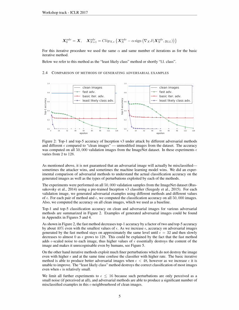
Figure 2: Top-1 and top-5 accuracy of Inception v3 under attack by different adversarial methodsand different ε compared to “clean images” — unmodified images from the dataset. The accuracywas computed on all 50, 000 validation images from the ImageNet dataset. In these experiments εvaries from 2 to 128.

As mentioned above, it is not guaranteed that an adversarial image will actually be misclassified—sometimes the attacker wins, and sometimes the machine learning model wins. We did an exper-imental comparison of adversarial methods to understand the actual classification accuracy on thegenerated images as well as the types of perturbations exploited by each of the methods.

The experiments were performed on all 50, 000 validation samples from the ImageNet dataset (Rus-sakovsky et al., 2014) using a pre-trained Inception v3 classifier (Szegedy et al., 2015). For eachvalidation image, we generated adversarial examples using different methods and different valuesof ε. For each pair of method and ε, we computed the classification accuracy on all 50, 000 images.Also, we computed the accuracy on all clean images, which we used as a baseline.

Top-1 and top-5 classification accuracy on clean and adversarial images for various adversarialmethods are summarized in Figure 2. Examples of generated adversarial images could be foundin Appendix in Figures 5 and 4.

As shown in Figure 2, the fast method decreases top-1 accuracy by a factor of two and top-5 accuracyby about 40% even with the smallest values of ε. As we increase ε, accuracy on adversarial imagesgenerated by the fast method stays on approximately the same level until ε = 32 and then slowlydecreases to almost 0 as ε grows to 128. This could be explained by the fact that the fast methodadds ε-scaled noise to each image, thus higher values of ε essentially destroys the content of theimage and makes it unrecognisable even by humans, see Figure 5.

On the other hand iterative methods exploit much finer perturbations which do not destroy the imageeven with higher ε and at the same time confuse the classifier with higher rate. The basic iterativemethod is able to produce better adversarial images when ε < 48, however as we increase ε it isunable to improve. The “least likely class” method destroys the correct classification of most imageseven when ε is relatively small.

We limit all further experiments to ε ≤ 16 because such perturbations are only perceived as asmall noise (if perceived at all), and adversarial methods are able to produce a significant number ofmisclassified examples in this ε-neighbourhood of clean images.

5

Workshop track - ICLR 2017

3 PHOTOS OF ADVERSARIAL EXAMPLES

3.1 DESTRUCTION RATE OF ADVERSARIAL IMAGES

To study the influence of arbitrary transformations on adversarial images we introduce the notionof destruction rate. It can be described as the fraction of adversarial images which are no longermisclassified after the transformations. The formal definition is the following:

d =

∑nk=1 C(X

k, yktrue)C(Xkadv, y

ktrue)C(T (X

kadv), y

ktrue)∑n

k=1 C(Xk, yktrue)C(X

kadv, y

ktrue)

(1)

where n is the number of images used to comput the destruction rate, Xk is an image from thedataset, yktrue is the true class of this image, and Xk

adv is the corresponding adversarial image. Thefunction T (•) is an arbitrary image transformation—in this article, we study a variety of transfor-mations, including printing the image and taking a photo of the result. The function C(X, y) is anindicator function which returns whether the image was classified correctly:

C(X, y) =

{1, if imageX is classified as y;0, otherwise.

We denote the binary negation of this indicator value as C(X, y), which is computed as C(X, y) =1− C(X, y).

3.2 EXPERIMENTAL SETUP

(a) Printout (b) Photo of printout (c) Cropped image

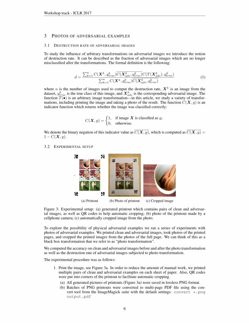
Figure 3: Experimental setup: (a) generated printout which contains pairs of clean and adversar-ial images, as well as QR codes to help automatic cropping; (b) photo of the printout made by acellphone camera; (c) automatically cropped image from the photo.

To explore the possibility of physical adversarial examples we ran a series of experiments withphotos of adversarial examples. We printed clean and adversarial images, took photos of the printedpages, and cropped the printed images from the photos of the full page. We can think of this as ablack box transformation that we refer to as “photo transformation”.

We computed the accuracy on clean and adversarial images before and after the photo transformationas well as the destruction rate of adversarial images subjected to photo transformation.

The experimental procedure was as follows:

1. Print the image, see Figure 3a. In order to reduce the amount of manual work, we printedmultiple pairs of clean and adversarial examples on each sheet of paper. Also, QR codeswere put into corners of the printout to facilitate automatic cropping.(a) All generated pictures of printouts (Figure 3a) were saved in lossless PNG format.(b) Batches of PNG printouts were converted to multi-page PDF file using the con-

vert tool from the ImageMagick suite with the default settings: convert *.pngoutput.pdf

6

Workshop track - ICLR 2017

(c) Generated PDF files were printed using a Ricoh MP C5503 office printer. Each pageof PDF file was automatically scaled to fit the entire sheet of paper using the defaultprinter scaling. The printer resolution was set to 600dpi.

2. Take a photo of the printed image using a cell phone camera (Nexus 5x), see Figure 3b.

3. Automatically crop and warp validation examples from the photo, so they would becomesquares of the same size as source images, see Figure 3c:

(a) Detect values and locations of four QR codes in the corners of the photo. The QRcodes encode which batch of validation examples is shown on the photo. If detectionof any of the corners failed, the entire photo was discarded and images from the photowere not used to calculate accuracy. We observed that no more than 10% of all imageswere discarded in any experiment and typically the number of discarded images wasabout 3% to 6%.

(b) Warp photo using perspective transform to move location of QR codes into pre-definedcoordinates.

(c) After the image was warped, each example has known coordinates and can easily becropped from the image.

4. Run classification on transformed and source images. Compute accuracy and destructionrate of adversarial images.

This procedure involves manually taking photos of the printed pages, without careful control oflighting, camera angle, distance to the page, etc. This is intentional; it introduces nuisance variabilitythat has the potential to destroy adversarial perturbations that depend on subtle, fine co-adaptationof exact pixel values. That being said, we did not intentionally seek out extreme camera anglesor lighting conditions. All photos were taken in normal indoor lighting with the camera pointedapproximately straight at the page.

For each combination of adversarial example generation method and ε we conducted two sets ofexperiments:

• Average case. To measure the average case performance, we randomly selected 102 imagesto use in one experiment with a given ε and adversarial method. This experiment estimateshow often an adversary would succeed on randomly chosen photos—the world chooses animage randomly, and the adversary attempts to cause it to be misclassified.

• Prefiltered case. To study a more aggressive attack, we performed experiments in whichthe images are prefiltered. Specifically, we selected 102 images such that all clean imagesare classified correctly, and all adversarial images (before photo transformation) are clas-sified incorrectly (both top-1 and top-5 classification). In addition we used a confidencethreshold for the top prediction: p(ypredicted|X) ≥ 0.8, where ypredicted is the class pre-dicted by the network for image X . This experiment measures how often an adversarywould succeed when the adversary can choose the original image to attack. Under ourthreat model, the adversary has access to the model parameters and architecture, so theattacker can always run inference to determine whether an attack will succeed in the ab-sence of photo transformation. The attacker might expect to do the best by choosing tomake attacks that succeed in this initial condition. The victim then takes a new photo of thephysical object that the attacker chooses to display, and the photo transformation can eitherpreserve the attack or destroy it.

3.3 EXPERIMENTAL RESULTS ON PHOTOS OF ADVERSARIAL IMAGES

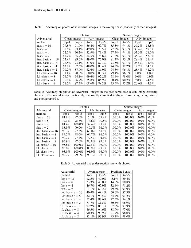
Results of the photo transformation experiment are summarized in Tables 1, 2 and 3.

We found that “fast” adversarial images are more robust to photo transformation compared to itera-tive methods. This could be explained by the fact that iterative methods exploit more subtle kind ofperturbations, and these subtle perturbations are more likely to be destroyed by photo transforma-tion.

One unexpected result is that in some cases the adversarial destruction rate in the “prefiltered case”was higher compared to the “average case”. In the case of the iterative methods, even the total

7

Workshop track - ICLR 2017

Table 1: Accuracy on photos of adversarial images in the average case (randomly chosen images).

Photos Source imagesAdversarial Clean images Adv. images Clean images Adv. imagesmethod top-1 top-5 top-1 top-5 top-1 top-5 top-1 top-5fast ε = 16 79.8% 91.9% 36.4% 67.7% 85.3% 94.1% 36.3% 58.8%fast ε = 8 70.6% 93.1% 49.0% 73.5% 77.5% 97.1% 30.4% 57.8%fast ε = 4 72.5% 90.2% 52.9% 79.4% 77.5% 94.1% 33.3% 51.0%fast ε = 2 65.7% 85.9% 54.5% 78.8% 71.6% 93.1% 35.3% 53.9%iter. basic ε = 16 72.9% 89.6% 49.0% 75.0% 81.4% 95.1% 28.4% 31.4%iter. basic ε = 8 72.5% 93.1% 51.0% 87.3% 73.5% 93.1% 26.5% 31.4%iter. basic ε = 4 63.7% 87.3% 48.0% 80.4% 74.5% 92.2% 12.7% 24.5%iter. basic ε = 2 70.7% 87.9% 62.6% 86.9% 74.5% 96.1% 28.4% 41.2%l.l. class ε = 16 71.1% 90.0% 60.0% 83.3% 79.4% 96.1% 1.0% 1.0%l.l. class ε = 8 76.5% 94.1% 69.6% 92.2% 78.4% 98.0% 0.0% 6.9%l.l. class ε = 4 76.8% 86.9% 75.8% 85.9% 80.4% 90.2% 9.8% 24.5%l.l. class ε = 2 71.6% 87.3% 68.6% 89.2% 75.5% 92.2% 20.6% 44.1%

Table 2: Accuracy on photos of adversarial images in the prefiltered case (clean image correctlyclassified, adversarial image confidently incorrectly classified in digital form being being printedand photographed ).

Photos Source imagesAdversarial Clean images Adv. images Clean images Adv. imagesmethod top-1 top-5 top-1 top-5 top-1 top-5 top-1 top-5fast ε = 16 81.8% 97.0% 5.1% 39.4% 100.0% 100.0% 0.0% 0.0%fast ε = 8 77.1% 95.8% 14.6% 70.8% 100.0% 100.0% 0.0% 0.0%fast ε = 4 81.4% 100.0% 32.4% 91.2% 100.0% 100.0% 0.0% 0.0%fast ε = 2 88.9% 99.0% 49.5% 91.9% 100.0% 100.0% 0.0% 0.0%iter. basic ε = 16 93.3% 97.8% 60.0% 87.8% 100.0% 100.0% 0.0% 0.0%iter. basic ε = 8 89.2% 98.0% 64.7% 91.2% 100.0% 100.0% 0.0% 0.0%iter. basic ε = 4 92.2% 97.1% 77.5% 94.1% 100.0% 100.0% 0.0% 0.0%iter. basic ε = 2 93.9% 97.0% 80.8% 97.0% 100.0% 100.0% 0.0% 1.0%l.l. class ε = 16 95.8% 100.0% 87.5% 97.9% 100.0% 100.0% 0.0% 0.0%l.l. class ε = 8 96.0% 100.0% 88.9% 97.0% 100.0% 100.0% 0.0% 0.0%l.l. class ε = 4 93.9% 100.0% 91.9% 98.0% 100.0% 100.0% 0.0% 0.0%l.l. class ε = 2 92.2% 99.0% 93.1% 98.0% 100.0% 100.0% 0.0% 0.0%

Table 3: Adversarial image destruction rate with photos.

Adversarial Average case Prefiltered casemethod top-1 top-5 top-1 top-5fast ε = 16 12.5% 40.0% 5.1% 39.4%fast ε = 8 33.3% 40.0% 14.6% 70.8%fast ε = 4 46.7% 65.9% 32.4% 91.2%fast ε = 2 61.1% 63.2% 49.5% 91.9%iter. basic ε = 16 40.4% 69.4% 60.0% 87.8%iter. basic ε = 8 52.1% 90.5% 64.7% 91.2%iter. basic ε = 4 52.4% 82.6% 77.5% 94.1%iter. basic ε = 2 71.7% 81.5% 80.8% 96.9%l.l. class ε = 16 72.2% 85.1% 87.5% 97.9%l.l. class ε = 8 86.3% 94.6% 88.9% 97.0%l.l. class ε = 4 90.3% 93.9% 91.9% 98.0%l.l. class ε = 2 82.1% 93.9% 93.1% 98.0%

8

Workshop track - ICLR 2017

success rate was lower for prefiltered images rather than randomly selected images. This suggeststhat, to obtain very high confidence, iterative methods often make subtle co-adaptations that are notable to survive photo transformation.

Overall, the results show that some fraction of adversarial examples stays misclassified even after anon-trivial transformation: the photo transformation. This demonstrates the possibility of physicaladversarial examples. For example, an adversary using the fast method with ε = 16 could expectthat about 2/3 of the images would be top-1 misclassified and about 1/3 of the images would betop-5 misclassified. Thus by generating enough adversarial images, the adversary could expect tocause far more misclassification than would occur on natural inputs.

3.4 DEMONSTRATION OF BLACK BOX ADVERSARIAL ATTACK IN THE PHYSICAL WORLD

The experiments described above study physical adversarial examples under the assumption thatadversary has full access to the model (i.e. the adversary knows the architecture, model weights, etc. . . ). However, the black box scenario, in which the attacker does not have access to the model, isa more realistic model of many security threats. Because adversarial examples often transfer fromone model to another, they may be used for black box attacks Szegedy et al. (2014); Papernot et al.(2016a). As our own black box attack, we demonstrated that our physical adversarial examples fool adifferent model than the one that was used to construct them. Specifically, we showed that they foolthe open source TensorFlow camera demo 2 — an app for mobile phones which performs imageclassification on-device. We showed several printed clean and adversarial images to this app andobserved change of classification from true label to incorrect label. Video with the demo availableat https://youtu.be/zQ_uMenoBCk. We also demonstrated this effect live at GeekPwn2016.

4 ARTIFICIAL IMAGE TRANSFORMATIONS

The transformations applied to images by the process of printing them, photographing them, andcropping them could be considered as some combination of much simpler image transformations.Thus to better understand what is going on we conducted a series of experiments to measure theadversarial destruction rate on artificial image transformations. We explored the following set oftransformations: change of contrast and brightness, Gaussian blur, Gaussian noise, and JPEG en-coding.

For this set of experiments we used a subset of 1, 000 images randomly selected from the validationset. This subset of 1, 000 images was selected once, thus all experiments from this section usedthe same subset of images. We performed experiments for multiple pairs of adversarial methodand transformation. For each given pair of transformation and adversarial method we computedadversarial examples, applied the transformation to the adversarial examples, and then computedthe destruction rate according to Equation (1).

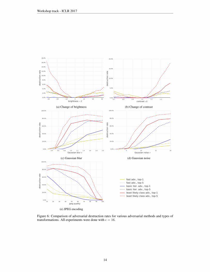
Detailed results for various transformations and adversarial methods with ε = 16 could be found inAppendix in Figure 6. The following general observations can be drawn from these experiments:

• Adversarial examples generated by the fast method are the most robust to transformations,and adversarial examples generated by the iterative least-likely class method are the leastrobust. This coincides with our results on photo transformation.

• The top-5 destruction rate is typically higher than top-1 destruction rate. This can be ex-plained by the fact that in order to “destroy” top-5 adversarial examples, a transformationhas to push the correct class labels into one of the top-5 predictions. However in order todestroy top-1 adversarial examples we have to push the correct label to be top-1 prediction,which is a strictly stronger requirement.

• Changing brightness and contrast does not affect adversarial examples much. The destruc-tion rate on fast and basic iterative adversarial examples is less than 5%, and for the iterativeleast-likely class method it is less than 20%.

2 As of October 25, 2016 TensorFlow camera demo was available at https://github.com/tensorflow/tensorflow/tree/master/tensorflow/examples/android

9

Workshop track - ICLR 2017

• Blur, noise and JPEG encoding have a higher destruction rate than changes of brightnessand contrast. In particular, the destruction rate for iterative methods could reach 80% −90%. However none of these transformations destroy 100% of adversarial examples, whichcoincides with the “photo transformation” experiment.

5 CONCLUSION

In this paper we explored the possibility of creating adversarial examples for machine learning sys-tems which operate in the physical world. We used images taken from a cell-phone camera as aninput to an Inception v3 image classification neural network. We showed that in such a set-up, a sig-nificant fraction of adversarial images crafted using the original network are misclassified even whenfed to the classifier through the camera. This finding demonstrates the possibility of adversarial ex-amples for machine learning systems in the physical world. In future work, we expect that it willbe possible to demonstrate attacks using other kinds of physical objects besides images printed onpaper, attacks against different kinds of machine learning systems, such as sophisticated reinforce-ment learning agents, attacks performed without access to the model’s parameters and architecture(presumably using the transfer property), and physical attacks that achieve a higher success rate byexplicitly modeling the phyiscal transformation during the adversarial example construction process.We also hope that future work will develop effective methods for defending against such attacks.

REFERENCES

Dzmitry Bahdanau, Kyunghyun Cho, and Yoshua Bengio. Neural machine translation by jointlylearning to align and translate. In ICLR’2015, arXiv:1409.0473, 2015.

Battista Biggio, Igino Corona, Davide Maiorca, Blaine Nelson, Nedim Srndic, Pavel Laskov, Gior-gio Giacinto, and Fabio Roli. Evasion attacks against machine learning at test time. In JointEuropean Conference on Machine Learning and Knowledge Discovery in Databases, pp. 387–402. Springer, 2013.

Nicholas Carlini, Pratyush Mishra, Tavish Vaidya, Yuankai Zhang, Micah Sherr, ClayShields, David Wagner, and Wenchao Zhou. Hidden voice commands. In 25thUSENIX Security Symposium (USENIX Security 16), Austin, TX, August 2016. USENIXAssociation. URL https://www.usenix.org/conference/usenixsecurity16/technical-sessions/presentation/carlini.

Nilesh Dalvi, Pedro Domingos, Sumit Sanghai, Deepak Verma, et al. Adversarial classification. InProceedings of the tenth ACM SIGKDD international conference on Knowledge discovery anddata mining, pp. 99–108. ACM, 2004.

Ian J. Goodfellow, Jonathon Shlens, and Christian Szegedy. Explaining and harnessing adversarialexamples. CoRR, abs/1412.6572, 2014. URL http://arxiv.org/abs/1412.6572.

Geoffrey Hinton, Li Deng, Dong Yu, George Dahl, Abdel rahman Mohamed, Navdeep Jaitly, An-drew Senior, Vincent Vanhoucke, Patrick Nguyen, Tara Sainath, and Brian Kingsbury. Deepneural networks for acoustic modeling in speech recognition. Signal Processing Magazine, 2012.

Alex Krizhevsky, Ilya Sutskever, and Geoffrey Hinton. ImageNet classification with deep convolu-tional neural networks. In Advances in Neural Information Processing Systems 25 (NIPS’2012).2012.

Blaine Nelson, Marco Barreno, Fuching Jack Chi, Anthony D Joseph, Benjamin IP Rubinstein,Udam Saini, Charles A Sutton, J Doug Tygar, and Kai Xia. Exploiting machine learning tosubvert your spam filter.

N. Papernot, P. McDaniel, and I. Goodfellow. Transferability in Machine Learning: from Phe-nomena to Black-Box Attacks using Adversarial Samples. ArXiv e-prints, May 2016b. URLhttp://arxiv.org/abs/1605.07277.

10

Workshop track - ICLR 2017

Nicolas Papernot, Patrick Drew McDaniel, Ian J. Goodfellow, Somesh Jha, Z. Berkay Celik, andAnanthram Swami. Practical black-box attacks against deep learning systems using adversarialexamples. CoRR, abs/1602.02697, 2016a. URL http://arxiv.org/abs/1602.02697.

Olga Russakovsky, Jia Deng, Hao Su, Jonathan Krause, Sanjeev Satheesh, Sean Ma, ZhihengHuang, Andrej Karpathy, Aditya Khosla, Michael Bernstein, et al. Imagenet large scale visualrecognition challenge. arXiv preprint arXiv:1409.0575, 2014.

Mahmood Sharif, Sruti Bhagavatula, Lujo Bauer, and Michael K. Reiter. Accessorize to a crime:Real and stealthy attacks on state-of-the-art face recognition. In Proceedings of the 23rd ACMSIGSAC Conference on Computer and Communications Security, October 2016. To appear.

Daniel F Smith, Arnold Wiliem, and Brian C Lovell. Face recognition on consumer devices: Re-flections on replay attacks. IEEE Transactions on Information Forensics and Security, 10(4):736–745, 2015.

Christian Szegedy, Wojciech Zaremba, Ilya Sutskever, Joan Bruna, Dumitru Erhan, Ian J. Goodfel-low, and Rob Fergus. Intriguing properties of neural networks. ICLR, abs/1312.6199, 2014. URLhttp://arxiv.org/abs/1312.6199.

Christian Szegedy, Vincent Vanhoucke, Sergey Ioffe, Jonathon Shlens, and Zbigniew Wojna. Re-thinking the inception architecture for computer vision. CoRR, abs/1512.00567, 2015. URLhttp://arxiv.org/abs/1512.00567.

11

Workshop track - ICLR 2017

AppendixAppendix contains following figures:

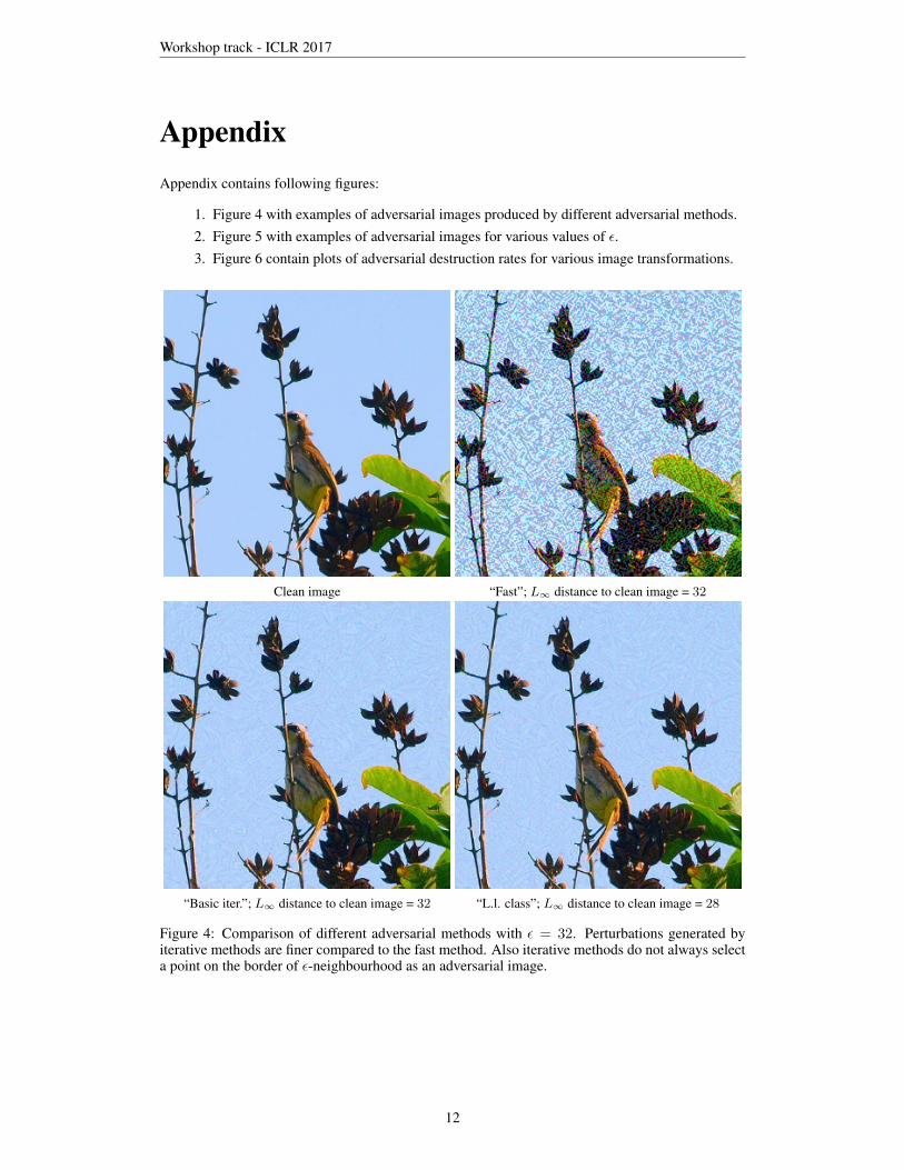
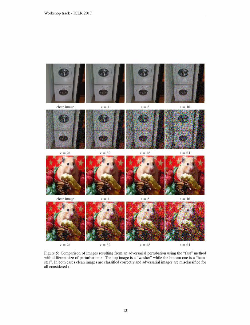
1. Figure 4 with examples of adversarial images produced by different adversarial methods.2. Figure 5 with examples of adversarial images for various values of ε.3. Figure 6 contain plots of adversarial destruction rates for various image transformations.

Clean image “Fast”; L∞ distance to clean image = 32

“Basic iter.”; L∞ distance to clean image = 32 “L.l. class”; L∞ distance to clean image = 28

Figure 4: Comparison of different adversarial methods with ε = 32. Perturbations generated byiterative methods are finer compared to the fast method. Also iterative methods do not always selecta point on the border of ε-neighbourhood as an adversarial image.

12

Workshop track - ICLR 2017

clean image ε = 4 ε = 8 ε = 16

ε = 24 ε = 32 ε = 48 ε = 64

clean image ε = 4 ε = 8 ε = 16

ε = 24 ε = 32 ε = 48 ε = 64

Figure 5: Comparison of images resulting from an adversarial pertubation using the “fast” methodwith different size of perturbation ε. The top image is a “washer” while the bottom one is a “ham-ster”. In both cases clean images are classified correctly and adversarial images are misclassified forall considered ε.

13

Workshop track - ICLR 2017

30 20 10 0 10 20 30

brightness +X

0.0%

2.0%

4.0%

6.0%

8.0%

10.0%

12.0%

14.0%

16.0%

18.0%

dest

ruct

ion r

ate

(a) Change of brightness

0.7 0.8 0.9 1.0 1.1 1.2

contrast ∗X

0.0%

5.0%

10.0%

15.0%

20.0%

dest

ruct

ion r

ate

(b) Change of contrast

0.4 0.6 0.8 1.0 1.2 1.4 1.6 1.8 2.0

Gaussian blur σ

0.0%

20.0%

40.0%

60.0%

80.0%

100.0%

dest

ruct

ion r

ate

(c) Gaussian blur

5 10 15 20

Gaussian noise σ

0.0%

20.0%

40.0%

60.0%

80.0%

100.0%

dest

ruct

ion r

ate

(d) Gaussian noise

10 20 30 40 50 60 70 80 90 100

Jpeg quality

0.0%

20.0%

40.0%

60.0%

80.0%

100.0%

dest

ruct

ion r

ate

(e) JPEG encoding

fast adv., top-1

fast adv., top-5

basic iter. adv., top-1

basic iter. adv., top-5

least likely class adv., top-1

least likely class adv., top-5

Figure 6: Comparison of adversarial destruction rates for various adversarial methods and types oftransformations. All experiments were done with ε = 16.

14