adverse selection and risk aversion in capital...
TRANSCRIPT

FinanzArchiv / Public Finance Analysis vol. 67 no. 4 1
Adverse Selection and Risk Aversion in CapitalMarkets
Luis H. B. Braido, Carlos E. da Costa, and Bev Dahlby*
Received 8 April 2009; in revised form 20 April 2011; accepted 3 September 2011
We generalize Boadway and Keen’s model of adverse selection in capital markets toallow for risk aversion on the part of entrepreneurs. We use the new model to ana-lyze two types of policies. We first consider policies that would allow entrepreneursto use a greater fraction of their total wealth in financing their projects, thus allow-ing them to reduce reliance on debt or equity finance by outside investors. We showthat such policies may not be welfare-improving, because they expose entrepreneurs tomore downside risk. This result highlights the importance of allowing for risk aversion,since policies that aim at alleviating inefficiencies associated with adverse selection mayincrease risk exposure and ultimately reduce welfare. We then consider how the taxtreatment of losses affects social welfare. We show that if a society places a high valueon distributional equity or if entrepreneurs are sufficiently risk-averse, a full-loss-offsetsystem may be desirable even when there is excessive investment.
Keywords: adverse selection, debt, equity, tax policy
JEL classification: H 20, G 14
1. Introduction
Since the 1970s, economists have recognized that capital markets do notalways conform to the model of an idealized market where individuals andfirms can always borrow funds at an interest rate that accurately reflectsthe degree of risk posed by their investment projects. One major sourceof capital market imperfection is asymmetric information between outsideinvestors and entrepreneurs. In many instances, entrepreneurs have betterinformation than outside investors about the probability that the investmentwill be successful, giving rise to a problem of adverse selection.
There is a good deal of controversy concerning the effect of adverse se-lection in economies with simple financial contracts, such as debt and equity.
* The authors are grateful for the helpful comments they received from seminar par-ticipants at the 2009 SBE meeting in Salvador. Carlos E. da Costa acknowledges thehospitality of MIT during the 2009–2010 academic year when part of this project wasdeveloped. He and Luis Braido acknowledge financial support from CNPq.
FinanzArchiv 67 (2011), 1--24 doi: 10.1628/001522111���ISSN 0015-2218 © 2011 Mohr Siebeck
Luis H. B. Braido, Carlos E. da Costa, and Bev Dahlby2
Two key papers in this literature – Stiglitz and Weiss (1981) and de Meza andWebb (1987) – focused on economies with a competitive debt market anddrew conflicting conclusions regarding the implications of adverse selectionfor investment. Stiglitz and Weiss concluded that adverse selection reducesinvestments and that resource allocation can be improved by subsidizingthe interest rates on loans. Using a modified version of that model that al-lows expected returns to vary across projects, de Meza and Webb concludedthat adverse selection results in excessive investment, in the sense that someprojects with an expected return that is below the opportunity cost of capitalwill be financed. Thus, resource allocation could be improved by taxing theinterest on loans.
Whether adverse selection coupled with debt–equity financial marketsleads to excessive or inadequate private investment has potentially import-ant implications for public policies, including tax policies. A symposium inthe February 2002 issue of The Economic Journal contained a number of the-oretical and empirical studies on the implications of asymmetric informationfor capital markets. In summarizing the debate, Cressy (2002) concluded thatgiven our current knowledge about the performance of capital markets, thebest advice that economists can give governments is “to do nothing,” that is,not to intervene by providing subsidies or imposing taxes.
Recent papers by Hellmann and Stiglitz (2000) and Boadway and Keen(2006) have extended the basic framework by allowing entrepreneurs tofinance their projects using either debt or equity from outside investors.1
Boadway and Keen (2006) showed that de Meza and Webbs (1987) excessive-investment result holds in an adverse-selection model with debt and equityfinancing, in which entrepreneurs and outside investors are both risk-neutral.
Boadway and Keen’s excessive-investment result challenges the prevailingview that capital market imperfections result in deficient investment, espe-cially by small startup firms. However, their assumption that entrepreneursare risk-neutral is troubling in that, at least in the conventional view, mostentrepreneurs are risk-averse and not able to hold a diversified portfolio ofassets. Their investment in their own firm represents the bulk of their wealth,and therefore they are exposed to a major source of risk if their firm shouldfail. Essentially, two sources of market failure could be operating at the sametime: adverse selection in a debt–equity capital market structure, which leadsto excessive investment in projects with negative net present values; and the
1 See also Fuest et al. (2003) and Fuest and Tillesen (2005) on adverse selection in cap-ital markets. Whereas Fuest and Tillesen (2005) explore occupational choice questions,Fuest et al. (2003) address the question of whether closed-end subsidies may characterizeoptimal policies when individuals are risk-neutral and markets present adverse-selectionproblems very similar to ours.

Adverse Selection and Risk Aversion in Capital Markets 3
entrepreneur’s inability to diversify risks, which leads to inadequate invest-ment in high-risk projects.
The risk-sharing possibilities in our model are exogenously restricted bythe types of financial contracts allowed in the economy, namely debt andequity. This restricted contract space is sometimes justified by the existenceof transaction costs that would prevent general mechanisms that were con-tingent on truthful announcements about the hidden characteristics of theproductive projects. We believe that our framework is an appropriate onefor representing capital markets in many economies, and that it providesuseful insights regarding economic policies that need to be assessed withinthe context of a model that incorporates those two sources of distortions,adverse selection and nondiversified risk.
There is now a large literature on the determination of entrepreneurship.Early contributions to this literature by Kihlstrom and Laffont (1979) andKanbur (1979) contain models of entrepreneurship where individuals differin their degree of risk aversion. In contrast, individuals in our model exhibitthe same degree of risk aversion and have the same amount of wealth. Theydiffer in the privately observed characteristics of their productive projects.This gives rise to an adverse-selection problem that is not captured in theseearly models of entrepreneurship.
It is not our intention to review the recent literature on entrepreneurship,but we do note that the recent paper by Jaimovich (2010) most closelyresembles our framework.2 In his overlapping-generations model, the onlyform of outside financing is equity investment. It only considers two types ofpotential entrepreneurs. Consequently, although Jaimovich’s model containsan interesting dynamic structure, it does not encompass the wider range offinancing possibilities and investment outcomes that our model considers anddoes not capture the possibility of equilibrium with excessive investment.
The remainder of the paper is organized as follows. In section 2, we gen-eralize Boadway and Keen’s model by allowing agents to be risk-averse.Simulations of the model in section 3 show that their excessive-investmentresult does not necessarily hold in this context. Total investment in riskyprojects declines with increasing degree of risk aversion, and there is a dis-tortion in the mix of projects that are financed. Some projects with relativelylow expected returns and negative net present values are financed, whileothers with positive net present values – but with high risk of failure – arenot undertaken.
In section 4, we consider two types of government policies that affect thevolume of investment and the types of projects that are financed. First, insection 4.1, we use the model to analyze the effects of policies that would
2 See also the recent work by Hopenhayn and Vereshchagina (2009).

Luis H. B. Braido, Carlos E. da Costa, and Bev Dahlby4
enable agents to utilize a larger fraction of their total wealth to financeinvestments. We show that such policies will have an ambiguous effect onthe expected utilities of entrepreneurs in that, while their interest paymentson debt financing will decline, they will be exposed to greater downside riskif their project fails. Agents endowed with high-risk, high-return projects aremost likely to be made worse off when more of their wealth has to be investedin a risky project. Consequently, investment in risky projects may decline,and social welfare may or may not increase. These numerical results arealigned with the theoretical underpinnings in our companion paper, Braidoet al. (2010), which considers an economy with debt financing only.
In section 4.2, we consider how the tax treatment of losses can affect thelevel of investment and compare the social welfare gains of tax systems witha full loss offset. Our simulations show that when entrepreneurs are risk-neutral and there is excessive investment, social welfare can be improvedby a reduction in the rate at which entrepreneurs are compensated for theirlosses combined with a revenue-neutral reduction in the tax on gains. (Thistax policy reduces investment in projects with high risk and low return.)However, our results also indicate that if a society places a high value ondistributional equity or if entrepreneurs are sufficiently risk-averse, a full-loss-offset system may be desirable even when there is excessive investment.
Our main results are then summarized and commented on in section 5,which serves as a conclusion.
2. A Model of Adverse Selection with Risk-Averse Entrepreneurs
The economy is inhabited by a continuum, with measure one, of agents,whose preferences are represented by expected-utility functions with iden-tical constant-relative-risk-aversion Bernoulli functions, given by
u(W) ≡{
W1−σ
1−σ for σ ≥ 0 and σ �= 1 ,
log(W) for σ = 1 ,(1)
where W ∈ R+ represents individual consumption wealth, and σ denotes thecoefficient of relative risk aversion.
All agents are potential entrepreneurs. Each of them is endowed witha project that requires one unit of wealth if it is to be realized. Projects arecharacterized by their probability of success, 0 < p ≤ 1, and by the magnitudeof their return if they are successful, R > 0. If the project is unsuccessful, thereturn is zero. Returns on the individual projects are uncorrelated, and agentsprivately know the characteristics (p, R) of their own projects.
This economy also has a continuum of potential outside investors whoseopportunity cost of capital is given by an exogenous risk-free real rate of

Adverse Selection and Risk Aversion in Capital Markets 5
return, r ≥ 0. Outside investors know the joint distribution of p and R acrossall projects and are aware that each agent is privately informed about thecharacteristics of his project, (p, R).
The agent’s wealth consists of two types of assets. One asset, L, cannotbe used to finance investment in the project. For example, L could be theearning of some family member or an asset that cannot be pledged as securityfor a loan because of legal restrictions or the absence of full property rights.The other asset, K, can be used to finance investment in the risky project.We assume that K < 1 and therefore the agent requires outside financing inorder to make the investment in his project. Define ϕ ≡ 1 − K > 0 as the levelof outside investment that is required to finance a project.
Debt Financing Let us first consider the case in which entrepreneurs canfinance their projects in a competitive debt market. The interest rate on debtfinancing for these projects is i ∈ R+. If the agent invests in the safe asset, hewill have a secure amount of wealth:
Ws ≡ L + (1 + r)K = L + (1 + r)(1 − ϕ) , (2)
where subscript s is used to indicate that the wealth, Ws, is secure.If an agent borrows to finance a project, his wealth is
W1B = max(L, R + L − (1 + i)ϕ) (3)
in case of success, and
W0B = L (4)
in case of failure. Subscript B indicates financing through borrowing; 0 de-notes the failure state, and 1 the success state.
Notice, however, that agents with R < (1 + i)ϕ will never apply for a loan,since this would imply a consumption level below Ws in all scenarios. Theexpected utility of a debt-financed entrepreneur can be written as
EUB = pW1−σ
1B
1 − σ+ (1 − p)
W1−σ0B
1 − σfor 0 ≤ σ �= 1 (5)
and
EUB = p log(W1B) + (1 − p) log(W0B) for σ = 1 . (6)
Agents will prefer debt-financing their projects to investing K in the safeasset if EUB ≥ W1−σ
s /(1 − σ). We can use (2) and (5)–(6) to define a func-tion Z(p) that partitions the space p × R, through (7), into two different sets:the locus (p,R) such that agents opt to become entrepreneurs (through debt-financing their projects); and the locus for which they opt not to do so. Thatis, agents choose debt financing over investing in the safe asset whenever
R ≥ Z(p) − L + (1 + i)ϕ , (7)

Luis H. B. Braido, Carlos E. da Costa, and Bev Dahlby6
where
Z(p) =[
W1−σs − (1 − p)L1−σ
p
] 11−σ
for 0 ≤ σ �= 1 (8)
and
Z(p) = L(
Ws
L
)1/p
for σ = 1 . (9)
The quantity Z(p) − L is always positive.3 Moreover, Z(·) is decreasingin p and increasing in σ. It can be interpreted as the level of wealth thatthe agent needs if the project succeeds in order to make the expected utilitywith a debt-financed investment equal to the utility from investing in the safeasset.
If the agents are risk-neutral, the inequality (7) can be written as
R ≥ (1 + r)(1 − ϕ)p
+ (1 + i)ϕ . (10)
Figure 1Boadway–Keen Equilibrium with Risk-Neutral Agents
In figure 1, which shows the Boadway–Keen equilibrium with risk-neutralagents, the BB′ curve represents the projects with (p, R) values such that
3 For that to be negative, one should have W1−σs
1−σ < p1−σ L1−σ + 1−p
1−σ L1−σ, which is impos-sible, since Ws > L.

Adverse Selection and Risk Aversion in Capital Markets 7
risk-neutral agents are indifferent between investing in their project usingborrowed funds and investing their wealth in the safe asset.
In equilibrium, competition among lending institutions implies that themarket interest rate on debt is determined by the following condition:
p ≡ E[p|R ≥ Z(p) − L + (1 + i)ϕ] = 1 + r1 + i
, (11)
where p is the average probability of success (and therefore repayment ofa loan) of debt-financed projects, r is the risk-free rate of return that thelending institutions pay to their depositors, and E[·] is the mathematical ex-pectation. (It is implicit in this reasoning that lending institutions hold a well-diversified portfolio of loans so that they can be treated as risk-neutral.)
Equity Financing Now consider equity financing by outside investors.Agents endowed with the project (p, R) can issue equity shares against theproject’s return. The number of shares issued by each firm is normalized toone. The price of each share, V, is given by the stock-market value of thefirm. All firms have the same equity value, since they are ex ante identicalfor outside investors.
Equity investors receive min(ϕ/V, 1) of the profits if the project is suc-cessful, and 0 otherwise. Equity-financed entrepreneurs, on the other hand,receive 1 − min(ϕ/V, 1) if the projects succeeds, and 0 otherwise. Their con-tingent wealth is
W1E = R[1 − min(ϕ/V, 1)] + L (12)
in case of success, and
W0E = L (13)
in case of failure. Subscript E denotes equity financing.The entrepreneur’s expected utility with equity financing, labeled E, is
given by
EUE = p1
1 − σW1−σ
1E + (1 − p)W1−σ
0E
1 − σfor 0 ≤ σ �= 1 (14)
and
EUE = p log(W1E) + (1 − p) log(W0E) for σ = 1 . (15)
Agents will use equity to finance their projects (instead of investing all theirresources in the safe asset) whenever
EUE ≥ W1−σs /(1 − σ) . (16)
Notice then that projects such that ϕ/V ≥ 1 will never be equity-financed.The inequality (16) can then be written as
R ≥ VV − ϕ
[Z(p) − L] , (17)
where Z(p) is as defined in (8).

Luis H. B. Braido, Carlos E. da Costa, and Bev Dahlby8
If the agent is risk-neutral, (17) can be written as
R ≥ VV − ϕ
(1 + r)(1 − ϕ)p
. (18)
The EE′ curve in figure 1 shows combination (p, R) values such that risk-neutral entrepreneurs are indifferent between equity financing and investingtheir wealth in the safe asset.
In equilibrium, investors bid up equity shares until
V = E[pR|R ≥ VV−ϕ
[Z(p) − L]]1 + r
. (19)
In words, the value of a firm is equal to the present value of its expectedreturn, conditional on equity financing, discounted at the risk-free rate ofreturn.
The Choice Between Equity and Debt Financing Some entrepreneursthat would be willing to use equity to finance their projects may actuallyprefer debt financing. Notice that, in our model, the entrepreneur’s degreeof risk aversion does not affect the preferred method of financing. This occursbecause entrepreneurs must always invest K > 0 from their own wealth inthe project.4 For the same reason, agents have no motivation for mixing debtand equity to finance a given project.
Debt financing is preferred to equity financing whenever EUE < EUB.From (5)–(6) and (14)–(15), this is equivalent to
pR(1 − (ϕ/V)) < p(R − (1 + i)ϕ) . (20)
From this reasoning, entrepreneurs are indifferent between debt and eq-uity financing when
R = (1 + i)V . (21)
The curve MM′ in figure 1 represents the projects for which agents are indif-ferent between debt and equity financing. An agent with a project whose Rlies below MM′ will prefer equity financing to debt financing.
It is important to notice that the BB′, EE′, and MM′ curves intersect atthe same point, namely,
pMEB = W1−σs − L1−σ
[(V − ϕ)(1 + i) + L]1−σ − L1−σfor 0 ≤ σ �= 1 (22)
and
pMEB = log(Ws) − log(L)log[(V − ϕ)(1 + i) + L] − log(L)
for σ = 1 .
4 This is equivalent to assuming that, in case of bankruptcy, the entrepreneurs are legallyresponsible for debts up to the amount K > 0.

Adverse Selection and Risk Aversion in Capital Markets 9
Moreover, when σ = 0, we have
pMEB = 1 − ϕ
V − ϕp . (23)
Therefore, entrepreneurs with projects whose (p, R) values lie above theline segment BJM′ in figure 1 will finance their projects with debt. Theprojects with relatively high R values are debt-financed so that the owners donot have to share the high returns with outside shareholders. Entrepreneurswith projects in the region JM′E′ will be financed in the stock market. Equityfinancing is attractive for agents with projects with relatively low R valuesand relative high probabilities of success.
The projects where the expected rate of return is greater than or equal tothe rate of return on the safe asset satisfy the condition pR > 1 + r. In figure 1,all of the projects that satisfy this condition lie on or above the FF ′ line. Theseare the projects that would be financed under symmetric information byrisk-neutral investors. The FF ′ line intersects the MM′ line at the probabilitylevel pMF defined by
pMF = pV
, (24)
where pMEB < pMF . Therefore, point A in figure 1 lies to the right of point J.
Market Equilibrium Equilibrium in this economy is given by an allocation– namely, three loci of projects (p,R) that are debt-financed, equity-financed,and not undertaken – and a vector of prices (i, V) such that agents maximizeexpected utility and the debt and equity markets satisfy the zero-profit condi-tions (11) and (19). As previously described, the individual optimal decisionsare summarized by the conditions (7), (17), and (20).
Figure 1 illustrates Boadway and Keen’s overinvestment result with risk-neutral agents. The debt-financed projects in the region BJAF will havea negative expected net present value because the FF ′ and the BB′ curvesintersect at the probability level p and FF ′ is steeper than BB′. Also notethat the EE′ curve is always below the FF ′ curve. In equilibrium, V is greaterthan one. (V can be interpreted as Tobin’s average q.) The equity-financedprojects in the region JE′F ′A will have negative expected present values.Thus, the Boadway–Keen model predicts that all of the projects with positiveexpected net present values will be financed and that some projects withnegative expected net present values will also be financed, either by debt orby equity.
If agents are risk-averse, it is possible that some projects with a positive netpresent value will not be financed. Intuitively, pMEB increases as the degreeof risk aversion increases – holding V and i constant – which shifts point J infigure 1 towards point A. This reduces the region of overinvestment. Note,
Luis H. B. Braido, Carlos E. da Costa, and Bev Dahlby10
however, that as the degree of risk aversion changes and poor projects aredropped, the equilibrium values for i and V will also change. Our intuitionsuggests that i will decrease and V will increase as risk aversion increases,which would have offsetting and therefore ambiguous effects on the positionof J and A. Therefore, an equilibrium analysis is required to assess the fulleffect of an increase in risk aversion on the level of overinvestment.
In addition to that, the slopes of the BB′ and EE′ curves will also changewhen agents become more risk-averse, creating the possibility that the BB′
curve may intersect the FF ′ curve above the MM′ line. Therefore, someprojects with low probabilities of success – but high returns and positivenet present values – will not be undertaken by agents, because they are toorisky.
In summary, when agents are risk-averse, some projects that should notbe undertaken will be undertaken, while some projects that should be un-dertaken will not be undertaken in equilibrium. The first type of inefficiencyoccurs for projects with high probability of success and low conditional re-turn, and the second for projects with low probability of success and highconditional return. Given the complexity of the model, it is not possible topin down the exact conditions leading to under- or overinvestment. We shallrely on numerical exercises to illustrate our results.
3. Equilibria with Excessive and with Inadequate Investment
We present here some numerical exercises in which the equilibrium exhibitseither excessive or inadequate levels of investment for different parame-ters. The model is simulated with the following parameter values: r = 0.05,ϕ = 0.60, L = 0.80, K = 0.40, and Ws = 1.22. The joint density function thatwe use to compute the equilibrium of the model is f (p, R) = θe−θR. With thisdensity, p has a uniform distribution for a given R, and R has an exponen-tial distribution for a given p. With θ = 1.25, we have p(R > 1) = 0.287,p(R > 2) = 0.082, E[p] = 0.5, E[R] = 0.80, E[pR] = 0.40. The area abovethe FF ′ curve is 0.095. This is the proportion of projects with positive netpresent values when they are evaluated at the risk-free rate of return andwould be equal to the proportion of the projects that would be undertakenby risk-neutral entrepreneurs with K = 1.
Table 1 shows the computed values of the key endogenous variables withthree different levels of risk aversion. In the first column, for comparativepurposes, we report the equilibrium values for the case with risk-neutralagents. In this case, the interest rate on debt is 63.1 percent. (One of thereasons why the interest rate is so high in this model is that we have as-sumed that the investment has no scrap value if it fails.) The market value

Adverse Selection and Risk Aversion in Capital Markets 11
Table 1
Equilibrium Simulations
Degree of Risk Aversion σ = 0 σ = 0.9 σ = 2.0
i 0.631 0.497 0.350V 1.109 1.109 1.096p 0.644 0.701 0.778pMEB 0.506 0.623 0.756
Percentage of projects financed by:Debt 7.24 7.23 6.68Equity 5.54 3.80 1.98Debt and Equity 12.8 11.0 8.66
Note: L = 0.8, K = 0.4, φ = 0.6, Ws = 1.22, r = 0.05, f (R) = 1.25e−1.25R
of the shares in the firms that are financed by equity investment is 1.109.The average probability that a debt-financed firm will repay its debt, p, is0.644. In other words, 35.6 percent of the debt-financed projects defaulton their loans. This also explains the high interest rate on debt in thismodel.
To simplify the diagrams we have omitted the part of the BB′ curve thatlies below the MM′ curve and the part of the EE′ curve that lies abovethe MM′ curve, because these sections of the curves are not relevant fordescribing the equilibrium when entrepreneurs can choose between debt andequity financing. We have combined the relevant sections of the BB′ and EE′
curves and relabeled this curve BE′. All of the projects that lie above the BE′
curve are financed either by debt or by equity. In the upper panel of figure 2the MM′ curve intersects the BE′ curve at the 0.506 probability level. Asnoted in the previous sections, excessive investment is a characteristic of theequilibrium with risk-neutral agents. About 7.24 percent of all projects arefinanced by debt, and 5.54 percent are financed by equity. The percentageof projects financed, 12.8 percent, exceeds the 9.5 percent that would befinanced if entrepreneurs were risk-neutral and had enough liquid wealth tofinance their own projects.
The second column presents the case in which the coefficient of relativerisk aversion is 0.90. In this case, the interest rate on debt drops to 49.7 per-cent, because the probability that a debt-financed entrepreneur will repay itsdebt increases to 0.701. The market value of shares in the firms that are fi-nanced by equity investment remains at 1.109. As the middle panel of figure 2shows, the MM′ and the BE′ curves now intersect at a much higher proba-bility level, 0.623. This equilibrium is characterized by both overinvestment

Luis H. B. Braido, Carlos E. da Costa, and Bev Dahlby12
Figure 2Equilibria with Excessive and Inadequate Investment
Adverse Selection and Risk Aversion in Capital Markets 13
and underinvestment. (The FF ′ curve lies above the BE′ curve in the rangeof p-values from about 0.22 to 0.60, and below the BE′ curve for p < 0. 22.)In other words, there is underinvestment in some projects with positive netpresent values and high risk because agents are unable to diversify the pro-ject’s risk. In this equilibrium, 7.23 percent of all projects are debt-financedand 3.80 percent are equity-financed. The percentage of projects financed,11.0 percent, exceeds the percentage that would have been undertaken byrisk-averse entrepreneurs with enough wealth to finance their own projects,5.18 percent.
In the third column, where the coefficient of relative risk aversion is 2.00,the interest rate on debt drops to 35.0 percent, because the probability thata debt-financed project will repay its debt increases to 0.778. The marketvalue of the shares in the firms that are financed by equity investment fallsslightly, to 1.096. As the last panel of figure 2 shows, the MM′ and BE′ curvesnow intersect at a higher probability level, 0.756. Now the equilibrium is char-acterized by underinvestment. The FF ′ curve lies almost completely belowthe BE′ curve, indicating significant underinvestment in projects with posi-tive net present values. Only 6.68 percent of all projects are debt-financed,and only 1.98 percent of projects are equity-financed. The percentage ofprojects funded, 8.66 percent, is less than the percentage with positive netpresent values but much higher than the 1.52 percent of projects that wouldbe taken by risk-averse entrepreneurs with enough liquidity to finance theirown projects. Thus, although the capital market is “imperfect,” more projectsare undertaken than would be if entrepreneurs had enough liquid wealth tofinance their own projects.
These simulations show that the excessive-investment result does not nec-essarily hold in a debt–equity capital market with adverse selection andrisk-averse agents. Our numerical simulations indicate that the number ofprojects that are financed can either exceed or fall short of the number thatwould be financed in a frictionless economy. What the model reveals is a dis-tortion in the mix of projects that are financed – some projects with lowexpected returns are financed, while some high-risk projects with positivenet present values are not.
It is important to emphasize that this is not a calibration exercise. That is,we did not choose parameters to try and match equilibrium values of sometarget variables. Instead, we chose functional forms and parameters that fa-cilitated both our exposition and the numerical computations. In particular,note that our choice of a zero scrap value for the project induces a counter-factually high value for interest rates. We do not believe that any of thesechoices are driving the underinvestment results. Indeed, underinvestment isfundamentally linked to the downside risk faced by entrepreneurs, which isnot directly affected by the equilibrium interest rate.

Luis H. B. Braido, Carlos E. da Costa, and Bev Dahlby14
4. The Welfare Effect of Government Policies
We investigate now the effects on social welfare of two different policies.First, we examine the effects of increasing the fraction of wealth that agentscan use in financing their projects. Our numerical exercise here concerns aneconomy with debt and equity markets.5
Second, we consider how the tax treatment of losses affects the level ofinvestment and social welfare in our setting.6 Many economists have arguedfor generous tax treatment of losses in order to promote risk-taking – seeDomar and Musgrave (1944), Mossin (1968), Stiglitz (1969), Mintz (1981),and Gentry and Hubbard (2000). However, most tax systems treat gains andlosses asymmetrically, with the tax rate on gains exceeding the rate at whichlosses are compensated. As our previous analysis has indicated, it is not clearwhether public policy should promote risktaking or discourage it with thosetypes of capital market distortions.
4.1. Increasing the Proportion of Wealth Available to Invest
An increase in K, with an offsetting reduction in L, has two effects on theincentive to invest in the risky project. First, the opportunity cost of investingin the risky project increases by rdK, and therefore some entrepreneurs withmarginal projects will find investing in the safe asset more attractive. Second,entrepreneurs will not have to borrow as much and their interest paymentswill decline, but at the same time they will face greater downside risk becauseof the reduction in L. Consequently, the expected utility of entrepreneursmay either increase or decrease.
To see this, we can write the expected utility of an entrepreneur witha debt-financed project as EUB = pU [R + L − (1 + i)ϕ]+ (1 − p)U(L), sincein equilibrium debt-financed projects display R > (1 + i)ϕ, as remarked insection 2. Hence, the effect on expected utility of an increase in K – holdingtotal wealth constant – is given by
ddK
EUB
∣∣∣∣W
> 0 iff i − ϕdi
dK>
1 − pp
U ′(R + L − (1 + i)ϕ)U ′(L)
, (25)
where di/dK is the change in the equilibrium interest rate on loans to en-trepreneurs and i − ϕdi/dK is the reduction in the entrepreneur’s interest
5 In a companion work, Braido et al. (2010), we derive similar theoretical results for aneconomy with debt financing only.
6 Kanbur (1982) and Kihlstrom and Laffont (1983) also deal with the effect of taxation onentrepreneurship, but their framework is quite different from ours. In particular, in theirmodels, risk-averse entrepreneurs face an uncertain production shock, but all potentialentrepreneurs face the same ex ante return. Thus, the adverse-selection problem does notarise in their models.

Adverse Selection and Risk Aversion in Capital Markets 15
payments from a small increase in K and an offsetting reduction in L, whichshifts wealth from the loss state to the success state of the world.
An entrepreneur’s marginal rate of wealth substitution between the twostates of the world is given by the right-hand side of the second set of condi-tions in (25). An entrepreneur will be better off if the reduction in his interestpayments exceeds his marginal rate of substitution of wealth between thetwo states of the world. For a given value of R, the entrepreneurs with low-pprojects have a higher marginal rate of substitution of wealth between thetwo states of the world and are more likely to be worse off when K increasesand L declines. Therefore, entrepreneurs with low-p projects are the onesthat are most likely to drop their projects. Consequently, the default rateon loans will decrease, and the interest rate on loans will decline, that is,di/dK < 0.
Holding p constant, the entrepreneurs with projects with higher R-valueswill have a higher marginal rate of wealth substitution, and therefore theyare more likely to be made worse off. Thus, somewhat paradoxically, reducedreliance on outside financing can make some entrepreneurs (with positive-net-present-value projects) worse off. Finally, the greater the degree of riskaversion, the higher is the marginal rate of wealth substitution, and the morelikely that an increase in K will make the entrepreneurs worse off.
It is important at this point to note the crucial role played by our assump-tion that the liability is the same for all entrepreneurs. We are, in this, rulingout the use of different levels of liability as a screening device. From a purelytechnical perspective, leaving the space of contracts to be limited only bythe informational structure of the economy leads to a series of difficultieswith regard to existence, let alone characterization. From a more practicalperspective, very complicated nonlinear contracts do not seem to be thecommon practice, at least for the type of small startup firms that underliesour risk-aversion assumption.
In our model, all individuals who purchase the safe asset have the sameexpected utility, but the entrepreneurs that finance their projects have ex-pected utilities that are greater than or equal to the expected utilities ofnoninvestors. In other words, all entrepreneurs who invest but the marginalones, who are indifferent by definition, get a surplus. Moreover, their utilitiesare increasing in both p and R. Distributional issues thus arise because non-investors and entrepreneurs have different expected utilities, and becausethere are differences in expected utilities among investors. An increase inthe amount of wealth that can be used to finance the projects, or an increasein loss offsets, will, in general, make some entrepreneurs better off and someworse off, because it will change the equilibrium interest rate and the priceof equity. Therefore, we have to be concerned about the distributional ef-fects of policy changes. To evaluate the distributional effects of a policy that

Luis H. B. Braido, Carlos E. da Costa, and Bev Dahlby16
increases K and reduces L, we will use the following social welfare function:
SWF =∫
p
∫R
(1 − �)−1E
[U(W)
]1−�f (p, R)dpdR , (26)
where � is the coefficient of inequality aversion. If � = 0, then the socialwelfare function is utilitarian. Our measure of social welfare is the equallydistributed equivalent (EDE), defined by
SWF = (1 − �)−1[U(EDE)]1−� . (27)
As demonstrated in our simulations in table 2, the level of investment maydecline when K increases and L declines. Entrepreneurs will be exposed tomore risk when they are responsible for financing a higher proportion of theinvestment, and the opportunity cost of investing in the risky project mayincrease.
Table 2
Increasing the Proportion of Wealth Available to Invest
Case I II III IV
Key Parameter Values L = 0.8 L = 0.4 L = 0 L = 0K = 0.4 K = 0.8 K = 1.2 K = 1.162ϕ = 0.6 ϕ = 0.2 ϕ = 0 ϕ = 0
Ws = 1.22 Ws = 1.24 Ws = 1.26 Ws = 1.22
i 0.497 0.308 na naV 1.109 1.165 na nap 0.701 0.803 na napMEB 0.623 0.782 na na
Percentage of projects financed byDebt 7.23 5.49 na naEquity 3.80 1.47 na naTotal 11.00 6.96 5.24 5.01
Equally dist. equivalent wealth� = 0 1.254573 1.267364 1.281950 1.240943� = 0.5 1.254159 1.267005 1.281655 1.240656� = 1.5 1.253357 1.266311 1.281083 1.240101
Note: σ = 0.90, r = 0.05, f (R) = 1.25e−1.25R
In case I, the entrepreneurs’ total wealth is 1.2, where L = 0.8 and K = 0.4.They must then rely on outside investors for 60 percent of the initial invest-ment. Assuming σ = 0.90, r = 0.05, and θ = 1.25, the equilibrium interest
Adverse Selection and Risk Aversion in Capital Markets 17
rate on loans would be 0.497, the value of a firm would be 1.109, and 11percent of the projects would be financed. In case I, with � = 0, the EDEwealth level is 1.254573. To put this figure in perspective, note that thoseentrepreneurs that invest in the safe asset and who have the lowest expectedutility have secure wealth equal to 1.22.
Case II shows the effect of reducing L from 0.8 to 0.4 and simultaneouslyincreasing K from 0.4 to 0.8. One could think of this increase in the amountof wealth that can be used to finance investments as arising from increas-ing property rights in informal housing in a developing country. Note thatthe entrepreneurs would still require outside financing for 20 percent of theproject’s cost. In the new equilibrium, the interest rate on loans would de-cline from 0.497 to 0.308, because the default rate on loans would declineby 10 percentage points (i.e., p would increase from 0.701 to 0.803). The de-cline in the default rate reflects the reduction in investment. In case II, only6.96 percent of the projects would be financed. Investment in the projects de-clines because the entrepreneurs’ secure level of wealth will have increasedto 1.24. Hence, some marginal projects will no longer be financed, becausethe opportunity cost of investing in the risky projects has increased. In add-ition, some entrepreneurs with positive-net-present-value projects will nowface a reduction in their expected utility from investing in their risky projects.
While the expected utilities of some of the entrepreneurs with goodprojects decline in case II, overall social welfare increases with a utilitar-ian or pro-poor social welfare functions because some of the losers wereinitially better off than the winners.
The next two cases analyzed assume that K > 1, so that entrepreneursmust self-finance their projects. In case III in table 2, the total wealth ofthe entrepreneurs is the same as in the previous cases, but they can nowself-finance the projects. Only 5.24 percent of the risky projects are financed,in part because Ws increases to 1.26, but also because of the increase in thedownside risk that the entrepreneurs face now that they finance the entireproject from their own wealth. However, there is an overall social welfaregain because of the increase in Ws to 1.26.
Case IV shows what would happen if in converting L into K, the valueof Ws remains constant, so that there is no gain for those who only invest inthe safe asset. The entrepreneurs can self-finance their investment, becauseK = 1.162. The computations show that only 5.01 percent of the risky projectswould be financed, even though the opportunity cost of the investment re-mains the same as in case I. This occurs because of the greater downsiderisk that the entrepreneurs face. The computed values of EDE wealth alsodecline.
We can use figure 3, which shows the equilibria in case I and case IV,to explain why social welfare declines when entrepreneurs can finance their
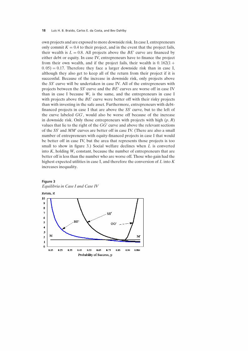
Luis H. B. Braido, Carlos E. da Costa, and Bev Dahlby18
own projects and are exposed to more downside risk. In case I, entrepreneursonly commit K = 0.4 to their project, and in the event that the project fails,their wealth is L = 0.8. All projects above the BE′ curve are financed byeither debt or equity. In case IV, entrepreneurs have to finance the projectfrom their own wealth, and if the project fails, their wealth is 0. 162(1 +0. 05) = 0.17. Therefore they face a larger downside risk than in case I,although they also get to keep all of the return from their project if it issuccessful. Because of the increase in downside risk, only projects abovethe SS′ curve will be undertaken in case IV. All of the entrepreneurs withprojects between the SS′ curve and the BE′ curves are worse off in case IVthan in case I because Ws is the same, and the entrepreneurs in case Iwith projects above the BE′ curve were better off with their risky projectsthan with investing in the safe asset. Furthermore, entrepreneurs with debt-financed projects in case I that are above the SS′ curve, but to the left ofthe curve labeled GG′, would also be worse off because of the increasein downside risk. Only those entrepreneurs with projects with high (p, R)values that lie to the right of the GG′ curve and above the relevant sectionsof the SS′ and MM′ curves are better off in case IV. (There are also a smallnumber of entrepreneurs with equity-financed projects in case I that wouldbe better off in case IV, but the area that represents those projects is toosmall to show in figure 3.) Social welfare declines when L is convertedinto K, holding Ws constant, because the number of entrepreneurs that arebetter off is less than the number who are worse off. Those who gain had thehighest expected utilities in case I, and therefore the conversion of L into Kincreases inequality.
Figure 3Equilibria in Case I and Case IV
Adverse Selection and Risk Aversion in Capital Markets 19
4.2. Tax Policy
Another type of public policy that affects investment decisions is the taxationof the returns on risky investments, and in particular, the tax treatment oflosses. We study next the tax treatment of losses for a simple linear taxsystem. We first provide a brief description of how taxes can be introducedinto our model. We then simulate the effects of varying the tax loss offsetsand compare the welfare gains and losses with a full-loss-offset tax system.
Let investment income be taxed at the rate τ, and investment losses reim-bursed at the rate t. A tax system with full loss offsets is one where τ = t.7
The return on the safe asset is then taxed at the rate τ, and if the individualhas invested in this asset, his wealth will be
W ′s = [1 + (1 − τ)r] (1 − ϕ) + L . (28)
For debt-financed or equity-financed projects, the entrepreneur’s wealthin state 0 (when the project fails) is given by
W ′0B = W ′
0E = L + (1 − ϕ)t . (29)
Note that we assume that the tax loss is restricted to the actual amount thatthe entrepreneur has invested in the project.
If the entrepreneur debt-finances a project that succeeds, his wealth be-comes
W ′1B = max{0, R − (1 + i)ϕ − τ(R − 1 − iϕ)} + L , (30)
where R − (1 + i)ϕ represents the return that the entrepreneur obtains afterpaying the principal and interest on loans, and τ(R − 1 − iϕ) is the tax pay-ment. It is assumed that the tax system allows the investor to fully depreciatethe initial investment and to deduct all of his interest payments. As wewill show later, debt-financed projects will always have the property thatR > 1 + iϕ, and therefore a successful debt-financed project will always be ina taxpaying position.
However, this may not be the case for an equity-financed project, if theproject is successful and R ≥ 1. Then, the entrepreneur’s wealth with anequity-financed project will be
W ′1E =
(V − ϕ
V
)R − τ(R − 1)
(V − ϕ
V
)+ L for R ≥ 1 , (31)
where the first term on the right-hand side is the entrepreneur’s share of thegross return on the project, and the second term is the entrepreneur’s shareof the taxes that have to be paid on the gain from the project. Again, weassume that the full cost of the project can be deducted from the return.
7 In practice, losses are not actually reimbursed, but the government allows the investorto carry them forward to reduce future tax liability. For multiproject firms, one can thinkthat there is loss offset at the project level.

Luis H. B. Braido, Carlos E. da Costa, and Bev Dahlby20
Note that it is also possible for an equity-financed project to be successfulbut incur a loss for tax purposes if 0 < R < 1. Thus, the entrepreneur’s wealthwill be
W ′1E =
(V − ϕ
V
)R + t(1 − R)
(V − ϕ
V
)+ L for 0 < R < 1 . (32)
The rest of the model follows the previous model with the addition of thesetax variables. The BB′ curve is implicitly defined by the equation W ′
1B = Z(p),and the EE′ curve is implicitly defined by W ′
1E = Z(p), where as before
Z(p) =[
W1−σs − (1 − p)[L + (1 − ϕ)t]1−σ
p
] 11−σ
. (33)
The MM′ curve is given by
RM = (1 + i)V − τ(1 + iV)1 − τ
. (34)
By virtue of entrepreneurial selection, the return of a debt-financed project,R, will always exceed RM. Thus, since ϕ < 1 < V, one must have R > 1 + iϕ.
Equilibrium in the debt market requires that the probability of success fora debt-financed project be equal to (1 + r)/(1 + i), while equilibrium in theequity market requires that the expected return of an outside investor equalthe after-tax return (1 − τ)r that it can earn on the safe asset.
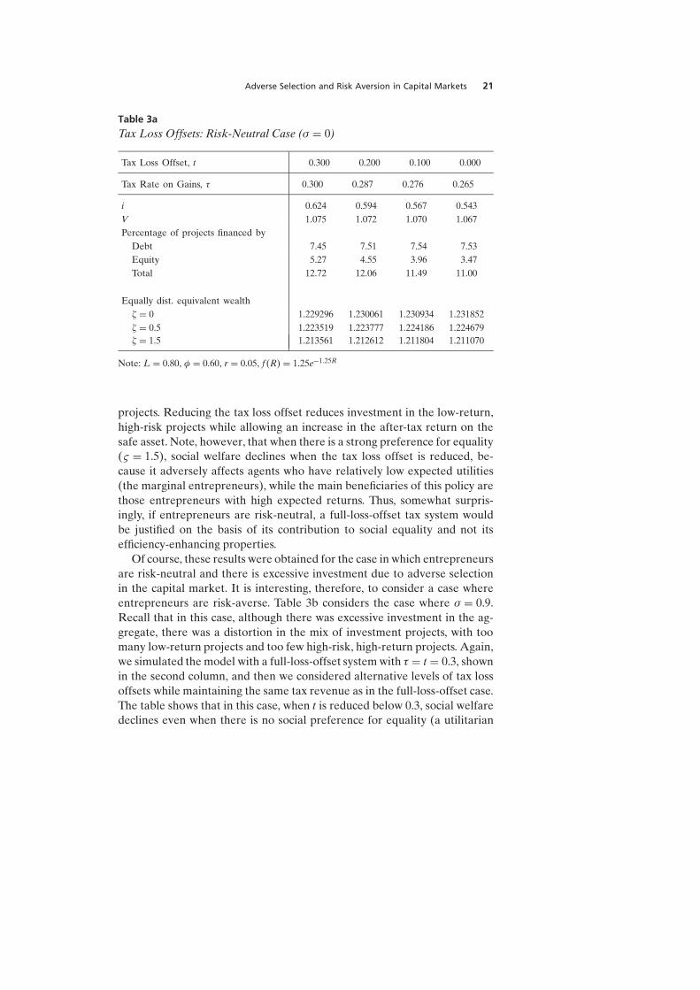
Table 3a illustrates how changes in the tax treatment of losses can affectinvestment in a debt–equity capital market with adverse selection. The firstcolumn shows the values of the key variables if entrepreneurs are risk-neutraland face a full-loss-offset tax system, where τ = t = 0.30. Note that the levelof total investment is virtually the same as in the equivalent no-tax case intable 1. Since there is excessive investment with risk-neutral entrepreneurs,it is interesting to examine the consequences of reducing t while holdingtotal tax revenues constant, which implies a reduction in τ. When the taxloss offset is reduced to 0.2 and the tax rate on gains can be reduced to0.287 while maintaining the same tax revenue as in the tax system with a fullloss offset, the total investment is reduced from 12.72 percent of all potentialprojects to 12.06 percent. (Note that there is a slight increase in the number ofdebt-financed projects, while the number of equity-financed projects declinessharply.) The interest rate and the value of a firm also decline.
We compute the certainty-equivalent wealth to measure the social gainsand losses from each of these revenue-neutral changes in the tax policy.When distributional equality is not important (i.e., ς = 0), social welfareincreases when the tax loss offset is reduced. The same result holds whenthere is a modest preference for distributional equity, namely ς = 0.5. Theimprovement in social welfare from reducing the tax loss offset should notbe surprising, because in this case there is excessive investment in risky
Adverse Selection and Risk Aversion in Capital Markets 21
Table 3a
Tax Loss Offsets: Risk-Neutral Case (σ = 0)
Tax Loss Offset, t 0.300 0.200 0.100 0.000
Tax Rate on Gains, τ 0.300 0.287 0.276 0.265
i 0.624 0.594 0.567 0.543V 1.075 1.072 1.070 1.067Percentage of projects financed by
Debt 7.45 7.51 7.54 7.53Equity 5.27 4.55 3.96 3.47Total 12.72 12.06 11.49 11.00
Equally dist. equivalent wealth� = 0 1.229296 1.230061 1.230934 1.231852� = 0.5 1.223519 1.223777 1.224186 1.224679� = 1.5 1.213561 1.212612 1.211804 1.211070
Note: L = 0.80, φ = 0.60, r = 0.05, f (R) = 1.25e−1.25R
projects. Reducing the tax loss offset reduces investment in the low-return,high-risk projects while allowing an increase in the after-tax return on thesafe asset. Note, however, that when there is a strong preference for equality(ς = 1.5), social welfare declines when the tax loss offset is reduced, be-cause it adversely affects agents who have relatively low expected utilities(the marginal entrepreneurs), while the main beneficiaries of this policy arethose entrepreneurs with high expected returns. Thus, somewhat surpris-ingly, if entrepreneurs are risk-neutral, a full-loss-offset tax system wouldbe justified on the basis of its contribution to social equality and not itsefficiency-enhancing properties.
Of course, these results were obtained for the case in which entrepreneursare risk-neutral and there is excessive investment due to adverse selectionin the capital market. It is interesting, therefore, to consider a case whereentrepreneurs are risk-averse. Table 3b considers the case where σ = 0.9.Recall that in this case, although there was excessive investment in the ag-gregate, there was a distortion in the mix of investment projects, with toomany low-return projects and too few high-risk, high-return projects. Again,we simulated the model with a full-loss-offset system with τ = t = 0.3, shownin the second column, and then we considered alternative levels of tax lossoffsets while maintaining the same tax revenue as in the full-loss-offset case.The table shows that in this case, when t is reduced below 0.3, social welfaredeclines even when there is no social preference for equality (a utilitarian

Luis H. B. Braido, Carlos E. da Costa, and Bev Dahlby22
Table 3b
Tax Loss Offsets: Risk-Averse Case (σ = 0.9)
Tax loss offset, t 0.400 0.300 0.200 0.100
Tax rate on gains, τ 0.313 0.300 0.290 0.282
i 0.570 0.528 0.492 0.460V 1.078 1.075 1.072 1.069Percentage of projects financed by
Debt 7.45 7.46 7.41 7.32Equity 4.96 4.05 3.33 2.76Total 12.41 11.51 10.74 10.08
Equally dist. equivalent wealth� = 0 1.210540 1.209368 1.208325 1.207188� = 0.5 1.209974 1.208678 1.207490 1.206174� = 1.5 1.208842 1.207289 1.205793 1.204090
Note: L = 0.80, φ = 0.60, r = 0.05, f (R) = 1.25e−1.25R
social welfare function). We also show in this table that social welfare in-creases if losses are compensated at a more generous rate than gains aretaxed, even though this implies that the tax rate on gains has to exceed 0.3 inorder to maintain total tax revenues at the full-loss-offset level. Of course,such generous tax treatment of losses would not be practical if losses wereaffected by entrepreneurial effort or if losses could be shifted within a corpo-rate group through transfer prices on intracorporate sales. However, thesecomputations do illustrate how important loss offset provisions can be insheltering entrepreneurs from risk when they are not able to hold diversifiedportfolios.
5. Conclusion
This paper builds on the framework of adverse selection in capital marketsanalyzed by Keen (2006). This class of models restricts the set of availablefinancial contracts to include only debt and equity. We stick with this marketstructure and extend the basic setup to allow for entrepreneurial risk aver-sion. We also introduce a secondary modification into the model – useful forpolicy analysis – that agents are guaranteed to retain the illiquid part of theirwealth in case of failure of their projects.
Boadway and Keen’s main result states that adverse selection coupledwith this capital market structure leads to excessive investment. We show

Adverse Selection and Risk Aversion in Capital Markets 23
that this result does not necessarily hold when entrepreneurs are risk-averse.This occurs because risk aversion introduces a new source of market failureinto the problem: while adverse selection (coupled with the debt–equitymarket structure) leads to excessive investment in projects with negativenet present values, the entrepreneur’s inability to diversify risk leads toinadequate investment in high-risk projects with positive net present values.
This framework is also used to evaluate a policy of varying the wealth thatentrepreneurs can use to finance investments. If institutional restrictionsdetermine the share of individual wealth that can be used as collateral, thena natural policy question is how varying this fraction would affect welfare.We show that freeing more resources need not always be welfare-improving.This may explain why many modern societies maintain restrictions on howone may use one’s own wealth.
We have also investigated the welfare implications of the tax treatment oflosses in this context. In debt–equity capital markets with adverse selection,there may be excessive investment in risky projects. Reducing the compensa-tion for losses may help to discourage investment in such projects, resultingin a social welfare gain if entrepreneurs are not too risk-averse or if societydoes not place an emphasis on distributional equality. However, our simu-lations show that full loss offsets may be justified, even in situations wherethere is excessive investment, if entrepreneurs are sufficiently risk-averse orif society places a high priority on distributional equality.
References
Boadway, R., and Keen, M. (2006), Financing and Taxing New Firms under AsymmetricInformation, FinanzArchiv / Public Finance Analysis 62, 471–502.
Braido, L. H. B., da Costa, C. E., and Dahlby, B. (2010), The Mystery of Capital underAdverse Selection: The Net Effects of Titling Policies, Fundacao Getulio VargasWorking Paper.
Cressy, R. C. (2002), Funding Gaps: A Symposium, Economic Journal 112, F1–F16.
de Meza, D., and Webb, D. (1987), Too Much Investment: A Problem of AsymmetricInformation, Quarterly Journal of Economics 102, 281–292.
Domar, E., and Musgrave, R. (1944), Proportional Income Taxation and Risk Taking,Quarterly Journal of Economics 58, 382–422.
Fuest, C., and Tillesen, P. (2005), Why Do Governments Use Closed Ended Subsidies toSupport Entrepreneurial Investment?, Economics Letters 89, 24–30.
Bernd H., and Tillesen, P. (2003), Tax Policy and Entrepreneurship in the Presence ofAsymmetric Information in Capital Markets, CESifo Working Paper No. 872.
Gentry, W., and Hubbard, G. (2000), Tax Policy and Entrepreneurial Entry, AmericanEconomic Review 90, 283–287.
Hellmann, T., and Stiglitz, J. (2000), Credit and Equity Rationing in Markets withAdverse Selection, European Economic Review 44, 281–304.

Luis H. B. Braido, Carlos E. da Costa, and Bev Dahlby24
Hopenhayn, H., and Vereshchagina, G. (2009), Risk Taking by Entrepreneurs, AmericanEconomic Review 99, 1808–1830.
Jaimovich, E. (2010), Adverse Selection and Entrepreneurship in a Model ofDevelopment, Scandinavian Journal of Economics 112, 77–100.
Kanbur, S. M. R. (1979), Of Risk Taking and the Personal Distribution of Income, Journalof Political Economy 87, 769–797.
Kanbur, S. M. R. (1982), Entrepreneurial Risk Taking, Inequality, and Public Policy: AnApplication of Inequality Decomposition Analysis to the General Equilibrium Effectsof Progressive Taxation, Journal of Political Economy 90, 1–21.
Kihlstrom, R., and Laffont, J. (1979), A General Equilibrium Theory of Firm FormationBased on Risk Aversion, Journal of Political Economy 87, 719–748.
Kihlstrom, R., and Laffont, J. (1983), Taxation and Risk Taking in General EquilibriumModels with Free Entry, Journal of Public Economics 21, 159–181.
Mintz, J. (1981), Some Additional Results on Investment, Risk Taking, and Full LossOffset Corporate Taxation with Interest Deductibility, Quarterly Journal of Economics96, 631–642.
Mossin, J. (1968), Taxation and Risk Taking: An Expected Utility Approach, Economica35, 74–82.
Stiglitz, J. (1969), Effects of Wealth, Income, and Capital Gains Taxation on Risk Taking,Quarterly Journal of Economics 83, 263–283.
Stiglitz, J., and Weiss, A. (1981), Credit Rationing in Markets with Imperfect Information,American Economic Review 71, 393–410.
Carlos E. da CostaFundação Getulio VargasGraduate School of EconomicsPraia de Botafogo, 19022250-900 Rio de [email protected]