Advertising for Attentionin a Consumer Search Model∗

Marco A. Haan† Jose Luis Moraga-Gonzalez‡

This version: March 2010

Abstract

We model the idea that when consumers search for products, they first visit the firm whoseadvertising is more salient. The gains a firm derives from being visited early increase insearch costs, so equilibrium advertising increases as search costs rise. This may resultin lower firm profits when search costs increase. We extend the basic model by allowingfor firm heterogeneity in advertising costs. Firms whose advertising is more salient andtherefore raise attention more easily charge lower prices and obtain higher profits. Asadvertising cost asymmetries increase, consumer surplus falls and aggregate profits rise.

JEL Classification Numbers: D83, L13, M37.

Keywords: consumer attention, consumer search, saliency enhancing advertising.

∗We thank Vaiva Petrikaite, Zsolt Sandor, Bert Schoonbeek, Chris Wilson and Jidong Zhou for theiruseful remarks. The paper has also benefited from seminar presentations at Catholic University Leuven,Copenhagen Business School, Erasmus University Rotterdam, Hebrew University of Jerusalem, IESE Busi-ness School, Tilburg University, University Pompeu Fabra and University of Valencia, and from conferencepresentations at ESEM 2009 (Barcelona), ASSET 2008 (Florence), University of Mannheim’s workshop on“The Economics of Advertising and Marketing” (Frankfurt, June 2008), EARIE 2007 (Valencia), and NAKEDay 2006 (Amsterdam). Moraga gratefully acknowledges financial support from Marie Curie Excellence GrantMEXT-CT-2006-042471.†Department of Economics and Econometrics, University of Groningen. E-mail: m.a.haan@rug.nl.‡ICREA, IESE and University of Groningen. E-mail: jose.l.moraga@gmail.com.

1

1 Introduction

Advertising is an important part of economic activity. In the US, for example, advertising

expenditures constitute around 2.2% of GDP. According to PriceWaterhouseCoopers (2005)

worldwide advertising in 2005 amounted to a staggering $385 billion. This amount is set to

grow to over half-a-trillion dollars in 2010. The outcome of such an impressive investment is

that the average citizen is exposed to hundreds of commercial messages every day.1 However,

very few of these messages are able to get through the clutter and raise the attention of

consumers.2

Part of the empirical marketing literature on advertising acknowledges that the primary

role of advertising is to create firm saliency, that is, the prominence of a brand or a shop in

consumers’ memories. This is more so given the (increasingly) large number of commercial

messages that consumers are confronted with every day. Enhancing the salience of a brand

or shop requires fine-tuning on a number of marketing variables. For example, Keller et

al. (1998) examine the effects of “suggestive” brand names on firm saliency;3 Unnava and

Burnkrant (1991) study the effects of advertising repetition on consumer memorability of a

brand or shop;4 finally, Burke and Srull (1988) and Alba and Chattopadhyay (1986) study

the existence of saliency enhancing advertising externalities and point out that investments

in “salience” of one firm inhibit the recall of alternative firms.

The economics literature (nicely surveyed in Bagwell, 2007) has focused on understanding

the implications of advertising for market outcomes. One branch of the literature considers

advertising as a sunk cost firms incur to enhance consumers’ willingness-to-pay for their

products. This has been coined persuasive advertising (see e.g. Braithwaite, 1928; Kaldor,

1950; Galbraith, 1967). It typically enhances perceived product differentiation and thus

softens competition. Since Telser (1964) and Nelson (1970, 1974), the view of advertising as

1Estimates of this number vary widely (see e.g. http://www.hhcc.com/?p=468 for a discussion). In 1972,Britt et al. (1972) already find between 300 and 600 messages per day. Arens et al. (2007), a popular textbook,even claims that ”as a consumer, you are exposed to hundreds and maybe even thousands of commercialmessages every day” (pg. 6).

2Franz (1986), for example, reports that out of more than 13,000 individuals questioned in 1985 about theadvertisements that were seen, heard or read in the past 30 days, 53 % were unable to remember any specificone.

3They report evidence that product/brand names explicitly conveying a product benefit or characteristicmay increase the recall probability of consumers interested in those characteristics. The name of the motorcycleTriumph Speed Triple may be a good example; this motorcycle is probably recalled more readily by consumersinterested in speedy and agile motorbikes. Another example is Sharp televisions.

4See also Janiszewski et al. (2003), who investigate the relationship between brand rehearsal, advertisingrepetition and advertising medium.

2

a device to transmit information has been gaining support. Through informative advertising,

firms can communicate, either directly or through signalling, their existence, location, price,

or quality. By increasing the information consumers possess, informative advertising typically

enhances competition.5

To the best of our knowledge, the economics of saliency enhancing advertising –i.e. ad-

vertising that increases shop and/or brand memorability without altering willingness-to-pay–

has not been considered so far. To close this gap, this paper proposes a model in which the

main role for the ads of a firm is to “compete” for the “attention” of consumers. The model

features firms that sell horizontally differentiated products and consumers who search shops

sequentially to find a product to their liking (see Wolinsky, 1986; Anderson and Renault,

1999). As search is costly, a consumer stops searching if she finds a deal that is attractive

enough to make an additional visit to a shop not worth her while. It is thus in the interest of a

firm to be visited earlier than the rivals, which gives a firm incentives to invest in saliency. We

assume that the order in which firms are sampled is influenced by how much they advertise.

More precisely, at every stage in the search process the probability that a consumer recalls a

shop and decides to visit it, is proportional to that shop’s share in total industry advertising.

Thus, advertising helps a firm to become more salient and to remind consumers of the kind

of products it sells. Whenever a consumer needs such a product, the firm hopes consumers

remember its shop more readily than those of its rivals.6

This model provides a suitable framework to understand the effects of search costs on

saliency enhancing advertising, product prices and firm profits. In addition, it provides a

rationale as to why consumers would increase their propensity to buy a product when they

see it advertised, without having to make the unsatisfactory assumption that advertising

directly increases willingness to pay, as is common in most models of persuasive advertising.

Finally, the model helps understand why there is so much advertising that conveys little

information about well-known horizontally differentiated brands/products.

5For advertising conveying direct information see e.g. Butters (1977), Shapiro (1980), Grossman and Shapiro(1984), Stahl (1994) and Bester and Petrakis (1995). For advertising as a signal of quality see Nelson (1974),Kihlstrom and Riordan (1984) and Milgrom and Roberts (1986). More recently, Anderson and de Palma(2008) study the effects of consumer limited attention on the production of messages and the emergence ofcongestion.

6In our model, advertising only provides information about the existence and location of shops, not aboutprices. The idea is that consumers have limited memory and by the time they go to the market they aresimply unable to remember all the prices they have seen in advertisements. The best an advertiser can hopefor is that consumers remember its identity and/or its location. In any case, there are many instances in whichadvertising prices is impractical. For example, when shops sell many products (like fashion shops, electronicssuperstores, supermarkets, etc.) it is simply unfeasible to list the prices of all products.

3

We find that both price and advertising expenditures increase in search costs. As search

costs increase, consumers are more reluctant to visit several shops. A typical shop then has

more market power over each consumer that does pay a visit, hence it charges a higher price.

At the same time, it becomes even more important for a firm to be salient and to be visited

early. Once a consumer visits a shop to inspect its product, she is less likely to walk away

to venture another shop. Hence a firm advertises more. The effect of an increase in search

costs on firm profitability is ambiguous. If search costs are relatively small, the price effect

dominates and equilibrium profits increase when search costs increase. However, when search

costs are relatively high, the price effect may be more than offset by the rent-dissipation effect

of increased advertising, so higher search costs may imply lower equilibrium profits. This is

contrary to the received wisdom in the literature on search costs (see e.g. the classic papers

of Reinganum, 1979; Burdett and Judd, 1983 and Stahl, 1989). Our model thus provides an

instance in which firms do not necessarily benefit from higher search costs. In fact, when

search costs are large enough, we show that firm profits can be lower than in a frictionless

world with zero search costs.

In our basic model, firms find themselves in a classic prisoners’ dilemma. If a firm adver-

tised less than the rest of the firms, the chance would be higher that this firm is pushed to

the end of consumers search order. In equilibrium all firms advertise with the same intensity

which implies that consumers end up recalling each firm with the same probability. Firms

would thus be better off if advertising were banned. From a welfare point of view, advertising

is purely wasteful so an advertising ban would be desirable.7

To study the effect of asymmetries, we provide an extension with two firms where one firm

is more efficient in generating saliency than the other. We find that the more efficient firm

advertises more and hence attracts a larger share of consumers on their first visit. This firm

also charges a lower price. By choosing to visit a second firm, consumers (indirectly) reveal

that they do no particularly like the product the first firm offered. Hence, such consumers

are less price-sensitive than consumers who still have the option to visit another shop. As the

less efficient firm’s pool of visitors has a higher share of these less price-sensitive consumers,

it finds it profitable to charge a higher price. Still, equilibrium profits of the more efficient

firm are higher. Advertising now has value for consumers as it helps them channel their first-

visits towards better deals. Nevertheless, because of the price increase of the less efficient

7Of course, if we take into account the advertising industry and we view advertising outlays as mere transfersfrom producers to advertisers, an advertising ban would be inconsequential.

4

firm, total consumer surplus is lower than in the case in which firms are visited randomly.

Savings in advertising outweigh consumer losses and overall welfare increases as advertising

cost asymmetries rise.8

As noted, we assume that the order in which firms are visited is influenced by advertising

efforts. In Hortacsu and Syverson (2004), sampling probability variation across firms is put

forward as a plausible explanation for the observed price dispersion in the mutual funds

industry. The authors use advertising outlays as one proxy for the sampling probability of a

fund in the market. Our model is consistent with that idea. Most theoretical papers in the

search literature assume that consumers sample firms randomly.9 Exceptions include the

following. In Arbatskaya (2007), the order in which firms are visited is exogenously given.

She finds that prices fall in the order in which firms are visited: a consumer that walks away

from a firm reveals that it has low search costs, which gives the next firm an incentive to

charge a lower price. In Wilson (2008), a firm can choose the magnitude of the search cost

consumers have to incur to visit it. In equilibrium, consumers are more likely to first visit

firms with low search cost and prices also fall in the search order. In our model firms sell

differentiated products which implies that prices increase in the (expected) order in which

they are sampled: a consumer that walks away from a firm has fewer (interesting) options

left and is thus less price sensitive. Finally, and more directly related to our specific model,

Armstrong et al. (2009) study a search market with differentiated products where one firm

is always visited first, while the other firms are sampled randomly if a consumer decides not

to buy from the prominent firm. In equilibrium, the prominent firm charges lower prices and

has higher profits than the other firms, for the same reason as in our analysis. Indeed, our

model can be interpreted as one in which firms invest in prominence but where prominence

can only be imperfect.

To capture the inhibition effects of saliency enhancing advertising, we depart from the

classical Butter’s (1977) technology and model advertising as a rent-seeking contest (Tullock,

1980). The theory of contests is extensive (for a survey, see Lockard and Tullock, 2001). In

most of this literature, agents’ valuations of the prize are independent of their efforts. By

8The welfare result is due to cuts in advertising expenditures. Therefore, if we took into consideration thefact that advertising outlays are not lost but transferred to the advertising industry, then overall welfare wouldbe lower than if advertising were banned altogether.

9See the seminal contributions of Rob (1985), Benabou (1993), Burdett and Judd (1983), Carlson andMcAfee (1983), Stahl (1989), Reinganum (1979) and Wolinsky (1986). More recent work includes Andersonand Renault (1999), Janssen and Moraga-Gonzalez (2004, 2007), Janssen et al. (2005) and Rauh (2004, 2007).

5

modeling the consumer search process and the pricing behavior of the firms, our paper adds to

this literature by proposing a game where valuations depend on advertising efforts and prices.

We prove existence of symmetric equilibrium for the n-person game and analyze asymmetric

equilibria in a two-person game.

Across industries, our model predicts a positive correlation between search costs, advertis-

ing expenditures and prices. Firms in an industry with higher search costs set higher prices,

but also advertise more. Within an industry, we predict a negative correlation between prices

on the one hand, and advertising expenditures and market shares on the other. Firms that

are more efficient in generating saliency attract more consumers, set lower prices and make

higher profits. Other papers also predict a negative relationship between advertising and

prices, but for different reasons. In Robert and Stahl (1993) firms can advertise prices on a

search market with homogeneous products, and advertise lower prices more intensively. In

Bagwell and Ramey (1994) advertising is used as a coordination device for firms to attract

more consumers and hence have lower costs, allowing them to charge lower prices. In our

model, firms that advertise more attract a pool of consumers that is more price sensitive, and

therefore charge lower prices.

The remainder of this paper is structured as follows. In section 2 we describe the set-up

of the model. The equilibrium results for symmetric firms are derived in subsection 3, and

the results on the effects of search costs on advertising efforts, prices and profits are given

in subsection 3.3. Section 4 presents results for a market with asymmetric firms. Section 5

concludes.

2 The model

There are n firms that sell horizontally differentiated products. Let N denote the set of

firms. Marginal costs are constant and normalized to zero. For simplicity and without loss

of generality we assume that there is one consumer. She has tastes described by an indirect

utility function

ui(pi) = εi − pi,

if she buys product i at price pi. The parameter εi is a match value between the consumer

and product i. Match values are independently distributed across products. We assume that

εi is the realization of a random variable with distribution F and a continuously differentiable

log-concave density f with support normalized to [0, 1]. No firm can observe εi so practising

6

price discrimination is not feasible. The consumer only learns εi upon visiting firm i. We

denote the monopoly price by pm, i.e., pm = arg maxp{p(1− F (p))}.

The consumer must incur a search cost s in order to learn the price charged by firm i as well

as her match value εi for the product sold by that firm. The consumer searches sequentially

with costless recall. We assume that search cost s is relatively small. In particular, we assume

that even if all firms charged the monopoly price, a consumer would still be willing to search,

that is,

0 ≤ s ≤ s ≡∫ 1

pm(ε− pm) f(ε)dε

Firms engage in an advertising battle to lure consumers to their shops. In particular we

assume that at any moment during the search process, a consumer is more likely to go to firm

i if she has had more exposure to the ads of that firm (or if the ads of firm i have happened

to be relatively more salient than other firms’ ads).10 The set-up of the model ensures that

the equilibrium does not have the consumer necessarily buying in the first shop she enters,

as is the case in most search models. Therefore, it is important for firms to be visited early,

but it is not crucial for making a sale.

Let ai, i = 1, 2, ..., n denote the number of advertisements of firm i. The cost of producing

ai advertisements is φi(ai), with φ′i > 0 and φ′′i ≥ 0. 11 Given an advertising strategy profile

(a1, a2, ..., an), suppose that the consumer has already visited v firms. Let V be the set of

visited firms. We assume that the probability that she will recall firm i ∈ N\V in the next

search is given byai∑

j∈N\V aj.

As opposed to the standard Butter’s (1977) technology, this modelling of the recall probability

captures the inhibition effects that own advertising has on the recall of competing brands (cf.

Burke and Srull (1988) and Alba and Chattopadhyay (1986)). A firm that does not advertise

at all is visited last. If no firm advertises, firms are sampled randomly.

This modelling of the consumer recall process is similar to that in the rent-seeking contest

described by Tullock (1980).12 Intuitively, one can think of each advertisement of a firm as a

10In the marketing and business literatures, the ease with which a brand/shop comes to mind is referred toas “top-of-mind awareness” (see e.g. Kotler, 2000).

11Alternatively, we may assume that firms decide on the amount Ai to spend on advertising, while theamount of ads of firm i is given by ai = τi(Ai). It is easy to see that this specification yields the exact sameoutcomes if we choose φi(·) = τ−1

i (·). The convexity of the advertising cost function is used only to ensureequilibrium existence and uniqueness (cf. Proposition 1); the other results hold for linear advertising costs.

12Schmalensee (1976) uses a similar idea in the context of advertising, but in his model prices are exogenouslygiven. Hortacsu and Syverson (2004), in their empirical study of price dispersion in the mutual fund industry,

7

ball this firm puts in an urn. Each firm can put as many balls in the urn as it likes. Whenever

the consumer needs a product, she draws one ball from the urn and visits the corresponding

firm. If, after the first visit, the consumer decides to visit another firm, she proceeds in the

same way: again draw a ball from the urn and visit the corresponding firm provided it has

not been visited yet; and so forth.13 We assume that the consumer cannot observe the levels

of advertising of firms, i.e. she does not observe how many balls each firm has put in the urn.

She only observes which ball she draws from the urn.

The timing in our model is as follows. First, firms simultaneously decide on advertising

and prices. Second, consumers sequentially search for a satisfactory deal following the recall

process described above. In Section 3.1 we focus on the case where all firms have the same

advertising technology i.e. where φi = φ, i = 1, 2, ..., n. In Section 4 we study a market where

firms differ in their advertising technologies.

3 Symmetric firms

3.1 Analysis

In this section we assume that all firms have the same advertising technology, denoted by φ.

We look for a symmetric Nash equilibrium. Consider firm i. Suppose that all firms different

from i charge price p∗ and set advertising level a∗. A symmetric Nash equilibrium then requires

that the best reply for firm i is to also set (a∗, p∗). To calculate firm i’s payoff, we need to

take into account the order in which firms may be visited, and the probability to make a sale

conditional on being visited.

Suppose that the buyer approaches firm i in her first search. This firm provides her with

net utility εi− pi. If εi− pi < 0, the consumer will search again. Suppose εi− pi ≥ 0. A visit

to some other firm j will yield εj − p∗. This is higher than the utility from buying from firm

i if εj > εi −∆, with ∆ = pi − p∗ ≥ 0. If we define x ≡ εi −∆, the expected benefit from

searching once more thus equals

g(x) ≡∫ 1

x(ε− x)f(ε)dε.

also model the funds’ sampling probabilities in a similar way. Chioveanu (2007) also uses this type ofadvertising technology in the context of persuasive (loyalty-inducing) advertising in a market for homogeneousproducts.

13See Skaperdas (1996) and Kooreman and Schoonbeek (1997) for axiomatizations of Tullock’s contest successfunction. An alternative formulation would be one where firms engage in an advertising race for consumers’attention (akin to the patent race models in the R&D literature). The results in Baye and Hoppe (2003) showthat these two formulations are strategically equivalent.

8

An additional search is worthwhile if and only if these incremental benefits exceed the cost

of search s. The buyer is exactly indifferent between an additional search and accepting the

offer at hand if x ≥ x, with x implicitly defined by

g(x) = s. (1)

The function g is monotonically decreasing. Moreover, g(0) =∫ 1

0 εf(ε)dε and g(1) = 0. It is

readily seen that s <∫ 1

0 εf(ε)dε. Therefore, for any s ∈ [0, s], there exists a unique x ∈ [pm, 1]

that solves (1).

Since any equilibrium necessarily has x ≥ p∗, the probability that a buyer stops searching

at firm i given that firm i is sampled, is equal to14

Pr[x > x and εi > pi] = Pr[x > x] = (1− F (x+ ∆)).

If we denote the probability that a consumer visits firm i in her first search and buys there

right away as λi1(ai, pi; a∗, p∗) we have:

λi1(ai, pi; a∗, p∗) =

aiai + (n− 1)a∗

(1− F (x+ ∆)) (2)

Now consider the case that a consumer goes to firm i in her second search and then decides

to buy there. This implies that she has visited some other firm first, say firm j, but decided

not to buy there. In the symmetric Nash equilibrium, whenever she walks away from a firm,

she expects price to be equal to p∗ in the next shop. The probability that she walks away

from j is thus given by Pr[εj < x ] = F (x). If we denote by λi2(ai, pi; a∗, p∗) the probability

that firm i is visited in second place and the consumer decides to buy from i right away, we

have

λi2(ai, pi; a∗, p∗) =

((n− 1) a∗

ai + (n− 1)a∗

)(ai

ai + (n− 2)a∗

)F (x)(1− F (x+ ∆)) (3)

where we have used the fact that the reservation value x is the same no matter how many

firms the consumer has already visited (see Kohn and Shavell, 1974). More generally, the

joint probability that a consumer visits firm i in her kth, k = 3, . . . , n search and buys there

right away is

λik(ai, pi; a∗, p∗) =

aiai + (n− k) a∗

k−1∏`=1

(n− `) a∗

ai + (n− `) a∗F (x)k−1 [1− F (x+ ∆)] . (4)

14This expression assumes that the deviation price pi is not too high, that is, 1 − F (x + ∆) is strictlypositive. Otherwise, no consumer would ever stop searching at firm i and, as a result, this firm would only sellto consumers who happen to find no acceptable product elsewhere. We come back to this issue in the proof ofProposition 1.

9

There is a probability that the consumer initially decides to walk away from firm i only to

find that, after having visited all firms in the industry, firm i offered the best deal after all. Of

course, the consumer will then return to firm i to buy there. The probability of this occuring

is

Pr[max{x,maxj 6=i{εj}} < x and εi − pi > max

j 6=i{εj − p∗} and εi > pi]

This probability is independent of the order in which firms are visited. We will denote it as

R(pi; p∗). Hence

R(pi; p∗) =

∫ x+∆

pi

F (ε−∆)n−1f(ε)dε. (5)

For pi close to p∗, we can now write firm i’s expected profits as

Πi(ai, pi; a∗, p∗) = pi

[n∑

k=1

λik(ai, pi; a∗, p∗) +R(pi; p

∗)

]− φ(ai). (6)

It is important to note that this expression is only valid for p close enough to p∗, i.e. for small

deviations from the tentative equilibrium (see footnote 14). For large deviations such that

F (x + ∆) = 1 the profit function looks different as the consumer would always walk away

from firm i, perhaps coming back to buy from it. We take this case into account in the proof

of the Proposition 1.15

Upon observing the payoff formulation in (6), it is clear our game differs from standard

rent-seeking games in two important respects. First, advertising is not a winner-takes-all

contest since after a consumer has visited a firm, she may still decide to go to a different

one. Second, because consumer search and prices are endogenous, the prizes obtained by the

winner, second winner, etc., all the way to the loser of the advertising contest depend in an

intricate way on the firms advertising efforts and prices.

Proposition 1 If a symmetric Nash equilibrium exists, advertising levels and prices are given

by the following system of equations:

a∗φ′(a∗)− p∗

n

(1− F (x)n −

n−1∑k=0

F (x)k(1− F (x)n−k

)n− k

)= 0 (7)

1− F (p∗)n

n+ p∗

(−f(x)

n

1− F (x)n

1− F (x)+

∫ x

p∗F (ε)n−1f ′(ε)dε

)= 0 (8)

Suppose that F represents the uniform distribution and that φ′′ is sufficiently large. Then a

symmetric equilibrium exists and is unique.

15Similarly, if a firm were to set an advertising effort arbitrarily close to zero, then the firm would be visitedlast with a probability arbitrarily close to one and then the payoff would be similar. In the Appendix we showthat these cases are not really problematic.

10

The proof of this result proceeds along the following lines. In step 1 we show that the

first order conditions imply the expressions (7) and (8). In step 2, we show that a solution to

this system of equations exists, and that it is unique if for example the distribution of match

values is uniform. Such a solution is indeed a symmetric Nash equilibrium if a firm cannot

profitably deviate when all other firms play (p∗, a∗). For general distributions functions F ,

however, the expression piR(pi; p∗) may not be quasi-concave in pi and so the profit Πi(·) may

be maximized at a pair other than (p∗, a∗). Under log-concavity of the density function f, the

expression piR(pi; p∗) is quasi-concave in pi (see Caplin and Nalebuff, 1991) but this does not

guarantee that Πi(·) is also quasi-concave in pi (since the sum of quasi-concave functions need

not be quasi-concave; see also Anderson and Renault, 1999). In step 3, we therefore focus on

the case where F is the uniform distribution and φ′′ is large. In that case, we show that the

payoff function Πi(·) is globally concave, so the solution to the system of equations(7) and (8)

is indeed the unique symmetric Nash equilibrium. In step 4, we show that large deviations

from (p∗, a∗), for which the profit function (6) is no longer the relevant one, are not profitable

either.

3.2 Comparative Statics

Proposition 2 The comparative statics of the equilibrium described in Proposition 1 are as

follows:

1. An increase in the marginal cost of advertising has no effect on equilibrium prices p∗

and lowers the equilibrium number of ads a∗.

2. If the density of match values is non-decreasing, an increase in search costs s raises

equilibrium price p∗ and raises the equilibrium number of ads a∗.

3. If match values are uniformly distributed, an increase in the number of firms n increases

per-firm advertising for n sufficiently low. In general, per-firm advertising goes to zero

as the number of firms approaches infinity.

Since all firms advertise with the same intensity in a symmetric equilibrium, changes

in advertising costs have no effect on equilibrium prices; these are only affected by relative

differences in advertising levels.16 Naturally, if advertising is more expensive, firms choose to

use less of it.16The fact that advertising costs do not affect equilibrium prices is an artifact of the symmetry of equilibrium.

Later in Section 4 we show how lowering the advertising cost of a firm results in a fall in its equilibrium price.

11

The result on the relationship between prices and search costs is similar to Anderson and

Renault (1999), who study a setting where the market is always fully covered in equilibrium,

in the sense that every consumer buys a product of one of the shops. Our result extends theirs

to a setting where industry demand is elastic. As search costs increase, the probability that a

consumer walks away from a firm to sample another one decreases. This confers market power

to firms that are visited and hence prices increase. The result on the relationship between

search costs and advertising is novel. An increase in search costs increases the market power

of a firm that is visited. Hence it becomes more desirable for a firm to attract that consumer.

As a result, firms advertise with greater intensity as search costs rise.

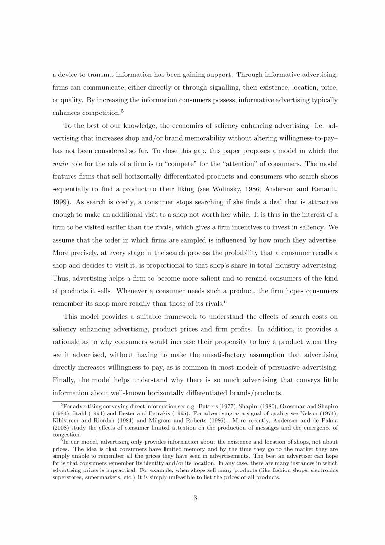
An increase in the number of firms has two effects on firms’ incentive to advertise. First,

if there are more firms that put out ads, the marginal effectiveness of an additional ad of firm

i decreases. This lowers the incentive to advertise. Second, as the number of firms increases,

it becomes more important to attract a consumer early. This raises the incentive to advertise.

If the number of firms is small, the second effect dominates. With many firms, the first effect

does. As the number of firms goes to infinity, a firm’s demand converges to zero so it is

impossible to support an equilibrium with advertising levels above zero. Figure 1 shows that

advertising intensity is non-monotonic in the number of firms for the uniform distribution

case. Prices and profits of the firms also decrease in n.

(a) Advertising intensity (b) Price

Figure 1: Price, advertising intensity and the number of firms

12

3.3 Profits and welfare

Search costs are generally seen as a boon to firms. As search costs increase, firms have more

market power, which leads to higher profits (see e.g. Reinganum, 1979; Burdett and Judd,

1983; or Stahl, 1989). The following result however shows that that is not necessarily true in

our model.

Proposition 3 Assume the advertising technology is linear. Then, the equilibrium effect of

search costs on firm profits is as follows:

1. For sufficiently small search costs s, profits increase in s.

2. For sufficiently large search costs s, profits may decrease in s and eventually fall below

the profits that firms would make in a frictionless world. In particular, this is true with

2 firms and uniformly distributed matching values.

An increase in search costs s has two opposite effects on firm profits. With an increase

in s, firms gain market power over customers that pay them a visit, which allows them to

charge a higher price. This tends to increase profits. But this also implies that it becomes

more attractive for each individual firm to attract consumers, to invest in saliency and try to

beat its rivals in the battle for attention. As a result, firms spend more on advertising, which

tends to lower firm profits. In our model, advertising is a rent-seeking activity that leads to

a dissipation of the rents generated by greater market power. When search costs are small,

the price effect dominates and firms gain from an increase in search costs. When search costs

are large, the advertising effect may dominate and profits decrease with higher search costs.17

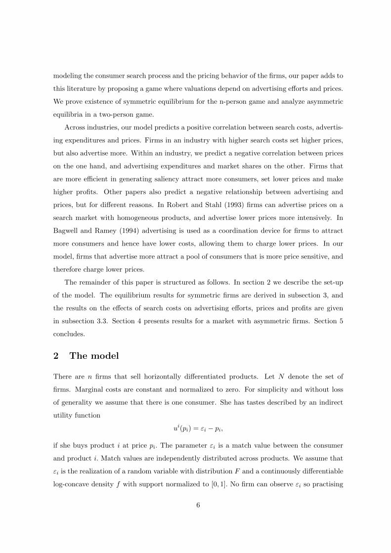
Interestingly, we may even have an overdissipation of rents in the sense firms spend more

resources to capture the additional rents than those rents are actually worth. This effect can

become so severe that firms end up obtaining profits that are lower than those in a world with

zero search costs. In Figure 2 we plot equilibrium profits against search costs. The dashed

lines show the profits firms would make if advertising were banned (a = 0), and the profits

firms would make if search costs were zero (s = 0).

In our model, lowering search costs always increases welfare. If the market were fully

covered, total welfare would be maximized if investments in advertising were minimized.

17It can be shown that this is not only true in the case described in the Proposition. It can also be shownto be true if the market is fully covered, as in Anderson and Renault (1999), or if the first search is costless,regardless of the number of firms and the distribution of matching values. Details are available from theauthors upon request.

13

Figure 2: Equilibrium profits (n = 2, f = 1, φ(a) = αa)

From Proposition 3, we know this to be the case if search costs are zero. Since we consider

a case in which industry demand is not completely inelastic, this result is only reinforced, as

lower search costs imply lower prices and hence a lower deadweight loss.18

Note that, in this model, firms find themselves in a prisoners’ dilemma. If a firm advertised

less than the rest, the chance that this firm is pushed to the end of consumers search order

would be higher. In equilibrium all firms advertise with the same intensity, which implies that

consumers end up recalling each firm with the same probability. Firms would thus be better

off if advertising were banned, while consumers would not be affected. From a welfare point

of view, advertising is purely wasteful.19 That is no longer true if we extend the model to

allow for asymmetric advertising technologies. In that case, the equilibrium will see has one

firm advertising more than the other. This implies that one firm is more likely to be visited

than the other, which in turn affects firms’ pricing incentives. We study this case in the next

section.

4 Asymmetric firms

The analysis in the previous section has ex-ante symmetric firms. This implies that in equi-

librium all firms that have not yet been visited by a given consumer, are always equally likely

18Interestingly, when search costs are sufficiently high, it would even be a Pareto improvement to have lowersearch costs. Consumers are better off as equilibrium prices decrease, while firms are better off as equilibriumprofits increase. Of course, here we are not taking into consideration the advertising industry. If we did,advertisers would lose as search costs fall (advertising expenditures are just transfers from the product marketto the advertising industry).

19Advertising does not add value in the product market. If we take into account the advertising industry andview advertising efforts as transfers from producers to advertisers, an advertising ban would be inconsequential.

14

to be visited next. Yet, it would be interesting to see how results are affected if firms are

no longer symmetric. Do firms that attract more consumers charge higher or lower prices?

More specifically, is higher advertising correlated with higher prices, or with lower ones? How

are consumer welfare and firm profits affected if consumers overwhelmingly visit firms in the

same order? We address such questions in this section.

To generate asymmetries between firms, we assume that they differ in their advertising

technology: for some exogenous reason, one firm is able to raise awareness at lower costs

than the other, for example because it runs a more effective advertising campaign, has a

more memorable shop’s name, or has a higher stock of advertising goodwill inherited from

the past.20 Technically, we assume that advertising cost φ differs between firms, so we write

φi(ai), i ∈ {1, 2}. Moreover, we assume that this is common knowledge.21 It turns out

that introducing asymmetries greatly complicates the analysis. We therefore have to restrict

ourselves to a setting with 2 firms and a uniform distribution of matching values. Even that

simple set-up does not allow us to always find analytical results, so we will partly have to

resort to a numerical analysis.

One complication has to do with consumer search behavior. Suppose that the equilibrium

has one firm charging a low price and one firm charging a high price. Consumers know

which prices are set in equilibrium. Suppose moreover that a consumer observes an out-of-

equilibrium price at her first visit. Her decision whether to continue searching will then be

affected by whether she interprets this out-of-equilibrium price as coming from the low-priced

firm or from the high-priced firm. One way to circumvent such complication is to assume

that, upon visiting a firm, a consumer can observe its advertising technology.22

4.1 Analysis

Let ω ∈ {1, 2, 12, 21} denote which firms a particular consumer visits, and in what order.

Thus ω = 12 implies that the consumer has first visited firm 1, and then firm 2. Let qωi

20Admittedly, there are alternative ways to introduce asymmetries across firms, for example the firms couldhave different marginal costs of production or offer different quality levels. We have chosen differences inadvertising costs because in the absence of advertising the equilibrium is still symmetric; this allows us tofocus on a case where the asymmetry in equilibrium prices stems only from differences in advertising levels.

21We have also explored the properties of an incomplete information game where the parameters of eachfirm’s advertising technology are drawn from the same uniform density function U(α). As shown by Fey (2008)for the simpler case where the prize is independent of the players’ efforts, the incomplete information problemis not tractable and can only be solved numerically.

22For example, from observing the lay-out and the colours in the store, she may realize that she has actuallyseen more ads from the other store and hence this store must be the one with the more costly advertisingtechnology.

15

denote total demand for firm i from such consumers. Thus q121 denotes demand for firm 1

from consumers that visit firm 1 and 2 in that order, while q11 denotes demand for firm 1 from

consumers that only visit firm 1. Denote with (a∗1, p∗1) and (a∗2, p

∗2) the equilibrium strategy

profile of the firms. In general, to study whether (a∗i , p∗i ) is a best reply to (a∗j , p

∗j ), with

i ∈ {1, 2}, j 6= i, we allow firm i to defect to some (ai, pi). Its profits then equal

πi = pi

(qii + qiji + qjii

)− φi(ai), (9)

where we have suppressed the arguments of the demand functions for ease of exposition. To

evaluate these profits, we first have to derive the relevant demand functions. Consider qii.

Suppose a buyer approaches i in her first search. This occurs with probability ai/(ai + a∗j ).

She then observes εi and pi. In equilibrium, she knows that a visit to j will yield utility εj−p∗j .

She benefits from such a visit whenever εj > εi − (pi − p∗j ) ≡ xi. Hence, her expected benefit

is∫ 1xi

(ε−xi)f(ε)dε. Recall that x is the solution to∫ 1x (ε− x)f(ε)dε = s. The probability that

this consumer immediately buys from firm i then equals23 Pr[xi > x] = 1 − F (x + pi − p∗j ).

Hence, using that F is a uniform distribution, we have

qii =ai

ai + a∗j

(1− x− pi + p∗j

). (10)

Next, qiji reflects a consumer that visits i first and finds an acceptable deal there, then decides

to also visit j, only to find that j provides her with a worse deal than i. Conditional on visiting

i first, the probability of this occurring is Pr[xi < x and εi − pi > εj − p∗j and εi > pi], hence

qiji =ai

ai + a∗j

∫ x+pi−p∗j

pi

(εi − pi + p∗j )dεi. (11)

Consider the consumer that visits j first. She observes a deal giving her utility εj − p∗j . At

firm i, this consumer expects to see a price equal to p∗i . If we define x∗j ≡ εj − p∗j + p∗i , the

probability she also visits i is Pr[x∗j < x]. Conditional on visiting j first, the probability that

a consumer buys from i therefore is Pr[x∗j < x and εi− pi > εj − p∗j and εi > pi]. This implies

qjii =a∗j

ai + a∗j

((x+ p∗j − p∗i ) (1− x− pi + p∗i ) +

∫ x+pi−p∗i

pi

(εi − pi + p∗j )dεi

)(12)

23Note that again, we must have x > p∗2, which implies that this probability is well-defined. We also assumethat x+ pi − p∗j ∈ (0, 1). In equilibrium, this is indeed the case.

16

Plugging (10), (11) and (12) into profits (9), we have:

πi = piai

ai + a∗j

(1− x− pi + p∗j +

1

2(x2 − p∗2j )

)+ pi

a∗jai + a∗j

((x+ p∗j − p∗i )(1− x− pi + p∗i ) +

1

2(x− p∗i )(x+ 2p∗j − p∗i )

)− φi(ai).

Taking the first order conditions with respect to own advertising intensity and price, and

imposing pi = p∗i and ai = a∗i we have, respectively:

0 = p∗ia∗j

(a∗i + a∗j )2

(1− x− p∗i + p∗j +

1

2(x2 − p∗2j )

)(13)

− p∗ia∗j

(a∗i + a∗j )2

((x+ p∗j − p∗i )(1− x) +

1

2(x− p∗i )(x+ 2p∗j − p∗i )

)− φ′i(ai)

0 =a∗i

a∗j + a∗j

(1− x− 2p∗i + p∗j +

1

2(x2 − p∗2j )

)(14)

+a∗j

a∗i + a∗j

((x+ p∗j − p∗i )(1− x− p∗i ) +

1

2(x− p∗i )(x+ 2p∗j − p∗i )

)Writing the conditions (13) and (14) for i = 1, 2 and j 6= i yields four nonlinear equalities

that can be solved to find equilibrium advertising levels and prices. From these first-order

conditions, we can prove the following results:

Proposition 4 With 2 firms, a uniform distribution of matching values, and asymmetric

advertising technologies, we have that the firm that advertises more, sets a lower price: a∗i > a∗j

necessarily implies p∗i < p∗j ;

This result can be understood as follows. By choosing to visit a second firm, consumers re-

veal that they do no particularly like the product the first firm offered. Hence, such consumers

are less price-sensitive than consumers who still have the option to visit another shop. The

firm with less advertising has a higher share of these less price-sensitive consumers. There-

fore, it finds it profitable to charge a higher price. This result is in line with the study of

Armstrong et al. (2009) on prominence. In their paper one firm, the prominent one, is visited

first for sure. Should the consumer decide to sample more firms, she does so at random. This

corresponds to the case in our model with advertising levels exogenously set to a∗1 > 0 and

a∗2 = 0.

17

4.2 Linear advertising technologies

To put additional structure on the model, we assume that advertising technologies are linear,

so φi(a) = αia. Moreover, we assume that firm 1 is more advertising-efficient than firm 2, in

the sense that raising additional awareness is always cheaper for firm 1 than it is for firm 2,

so α1 < α2. It is then easy to show that firm 1 will advertise more:

Proposition 5 In equilibrium, the more advertising-efficient firm will advertise more.

4.3 Numerical analysis

To do comparative statics we have to resort to a numerical analysis. We again assume linear

advertising technologies. Without loss of generality, we assume that firm 1 has the more

efficient advertising technology, and normalize α2 to 1, so α1 ≤ α2 < 1. From the analysis

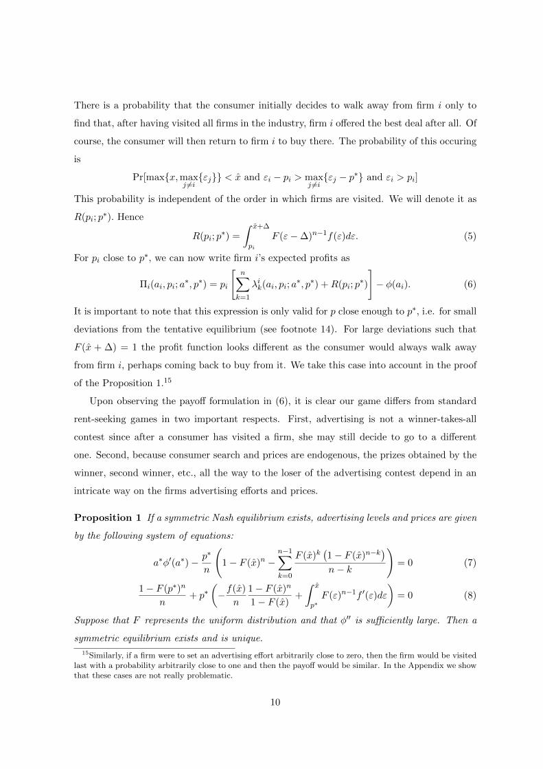
above in Section 4.1 we know that this implies that a∗1 ≥ a∗2 and p∗1 ≤ p∗2. The parameter

α ≡ α1 now reflects the extent of asymmetry between advertising technologies: as α increases,

advertising technologies become more symmetric.

(a) Price (b) Advertising intensity

Figure 3: Price, advertising intensity and the number of firms

In Figure 3 we depict equilibrium prices and advertising levels as a function of α. For the

level of search costs, we have chosen s = 0.08, but changing this value does not affect these

graphs qualitatively.

18

Result 1 With 2 firms, a uniform distribution of matching values, linear advertising tech-

nologies, and firm 1 the more advertising-efficient firm, we have the following:

1. if we denote by (a∗s, p∗s) equilibrium advertising levels and prices in case of equal adver-

tising technologies, then p∗1 < p∗s < p∗2.

2. an increase in the asymmetry in firm advertising efficiency has the following effects:

(a) the price of the cheapest firm decreases, that of the most expensive firm increases,

while average prices also increase;

(b) the advertising level of the cheapest firm increases, that of the most expensive firm

decreases, while average advertising levels also increase.

The first result confirms the intuition behind Proposition 4: the cheaper firm also charges a

lower price than what it charges with equal advertising, while the more expensive firm charges

a price that is also higher than what it charges with equal advertising. Result 2a shows that

the price gap becomes more pronounced as the difference in equilibrium advertising levels

increases. Result 2b implies that, as the asymmetry in firm advertising costs increases, the

difference in advertising efforts will also increase.

Note that a firm that advertises more, is more likely to be visited first by a consumer. As

she knows that this firm charges a lower price than the other firm, she is also less likely to

walk away from this firm. This suggests that the number of equilibrium searches will be lower

when there is more asymmetry between advertising levels of the two firms. The following

result establishes that this is indeed the case.24

Result 2 With 2 firms, a uniform distribution of matching values, and linear advertising

24If we take the results in Result 1 as given, we can also establish this result formally. By construction, eachconsumer searches at least once for sure. If she visits i first, the probability of a second search is F

(x+ p∗i − p∗j

).

If she visits j first, the probability of a second search is F(x+ p∗j − p∗i

). Denote γ ≡ a∗i /

(a∗i + a∗j

). We can

write the expected number of searches as

E(searches) = 1 + γ(x+ p∗i − p∗j

)+ (1− γ)

(x+ p∗j − p∗i

)= 1 + x+ (1− 2γ)

(p∗j − p∗i

)The results in Proposition 1 imply that ∂p∗2/∂γ > 0 and ∂p∗1/∂γ < 0, so

∂E(searches)

∂γ= −2

(p∗j − p∗i

)+ (1− 2γ)

(∂p∗j∂γ− ∂p∗i

∂γ

)< 0.

Hence the number of searches decreases as γ increases, that is, if the asymmetry between equilibrium advertisinglevels increases.

19

technologies, we have that the number of searches, and hence total search costs incurred by

consumers, decreases as the asymmetry in advertising levels increases.

Hence, advertising now has social value as it helps consumers to channel their first-visits

towards better deals.

4.4 Welfare

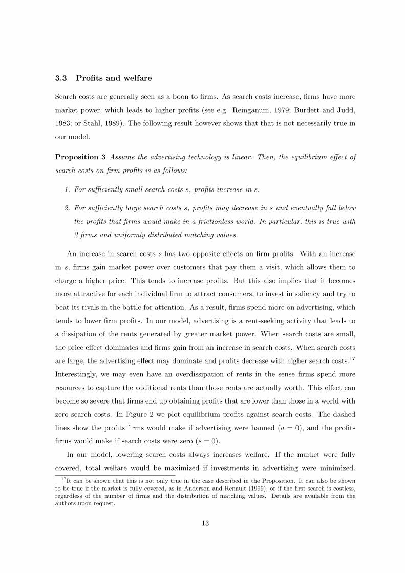
Consumer welfare will depend on where a consumer buys, and which firms she visits. In

Figure 4, we have depicted this in (ε1, ε2)-space. The left-hand panel gives the analysis for

consumers that first visit firm 1, the right-hand panel reflects consumers that first visit firm

2. In the left-hand panel, the dark-shaded area reflects the consumers that immediately buy

from 1. Consumers in the vertically dashed area also buy from 1 – but only after having

visited both firms. Consumers in the horizontally dashed area buy from 2 after having visited

both firms. Consumers in the white bottom-left corner do not buy at all.

(a) First visit firm 1 (b) First visit firm 2

Figure 4: Consumer purchasing behavior

In the right-hand panel, consumers in the vertically dashed area again buy from 1, and

consumers in the horizontally dashed area from 2, both after having visited both firms. Con-

sumers in the lightly shaded area buy from 2, consumers in the white area do not buy at

all.

20

Consider an increase in advertising asymmetry. The first effect of this is that total adver-

tising of firm 1 increases, hence the left-hand panel of firm 1 will become relevant for more

consumers. This effect is beneficial for consumer welfare, as more consumers now visit the

cheaper firm first. Next, p∗1 decreases while p∗2 increases. This implies for the left-hand panel

that the lines ε1 = p∗1 and ε1 = x+ p∗1 − p∗2 move to the left, while the lines ε2 = ε1 + p∗2 − p∗1and ε1 = p∗2 move upwards. Consumers that already bought from 1, or switch their choice to

1, benefit. The total number of searches decreases. Consumers that still buy from 2, however,

are hurt, while numerical simulations show that the total number of non-buyers also increases.

The effects in the right-hand panel are similar.

In sum, as asymmetry between advertising technologies increases (so α1 decreases), the

price of 1 decreases while that of 2 increases. The first effect is good news for consumers,

also as they visit 1 more frequently than 2. However, as 2’s price is higher, consumers who

fail to find a satisfactory product at 1 are forced to accept a (much) higher price more often.

On average consumers search less, which lowers their search costs but also makes them less

exposed to variety. The total number of consumers who buy decreases, which is obviously a

source of inefficiency. The aggregate effect on consumer welfare is therefore complex.

To calculate consumer surplus, we use the same notation as above: we let ω ∈ {1, 2, 12, 21}

denote which firms a consumer has visited, and in what order. Thus ω = 12 implies that

this consumer has first visited firm 1, and then firm 2. Let CSωi denote the total surplus of

such consumers who buy from firm i. Consider, for example, consumers that buy from i that

have only visited i. These consumers each incur total search costs s. Their net surplus thus

is εi − p∗i − s. Moreover, they have εi > x− p∗j + p∗i . Hence

CSii =

∫ 1

0

∫ 1

x−p∗j+p∗i

(εi − p∗i − s)dεidεj

Similarly,

CSiji =

∫ x−p∗j+p∗i

p∗i

∫ εi+p∗j−p∗i

0(εi − p∗i − 2s)dεjdεi

CSijj =

∫ 1

x

∫ x−p∗j+p∗i

0(εj − p∗j − 2s)dεidεj +

∫ x

p∗j

∫ εj−p∗j+p∗i

0(εj − p∗j − 2s)dεidεj

Ex-ante expected consumer surplus then equals:

CS =a∗1

a∗1 + a2(CS1

1 + CS121 + CS12

2 ) +a∗2

a∗1 + a2(CS2

2 + CS212 + CS21

1 )

21

Figure 5: Welfare

and total welfare is W = CS + Π∗1 + Π∗2 as usual.

To fully appreciate the effect of a change in α on welfare, we have to resort to numerical

analysis. In figure 5, we depict the components of total welfare equilibrium profits of firm

1 and 2, as a function of α, for the case that s = 0.08. For different levels of s, the picture

looks qualitatively the same. We can see that profits of firm 1 decrease as firms become

more symmetric, while profits of firm 2 increase – but less so. Total profits thus decrease.

From the figure, it is hardly discernible that consumer welfare increases as firms become more

symmetric. Thus, the net effect of a decrease in α is for consumer welfare to go down, but

this effect is very small.25 Total welfare goes up as firms become more asymmetric. This is

driven by the increase in the profits of firm 1 along with savings in search and advertising

costs.26

Simulations show that the comparative statics with respect to search costs are qualitatively

unaffected by the asymmetry of advertising technologies.27 For given advertising asymmetry

α, total advertising is still increasing in search costs s. Equilibrium advertising levels of both

firms increase in s, as do prices. Profits of firm 1, the most advertising efficient firm, are

non-monotonic in s: initially they increase, but for high enough s they decrease. The same

is true for firm 2. Total welfare decreases in search costs, as does consumer welfare.

25For this particular parametrization, total consumer welfare falls by less than 1% as α changes from 1 to0.1. If we set search costs equal to 0.02 rather than 0.08, exactly the same is true.

26The welfare result is not only driven by the fact that firm 1 has access to a more efficient advertisingtechnology. In fact we obtain also a welfare gain if we introduce asymmetries by increasing rather thandecreasing the marginal cost of advertising of firm 1.

27Details are available from the authors upon request.

22

5 Conclusion

Firms engage themselves in a battle for attention in an attempt to being visited as early

as possible in the course of search of a consumer. Through investments in more appealing

advertising, a firm can achieve a salient place in consumer memories. Consumers will then

visit this firm sooner than the rival firms. We modelled this idea in the framework of a model

of search with differentiated products. In such a framework, advertising is not a winner-takes-

all contest: after a consumer has visited a firm, she may still decide to go to a different one

if she does not sufficiently like the product of the current particular firm.

We found that prices and advertising levels are increasing in consumers’ search costs. Yet,

the effect on profits is ambiguous. If search costs are small to start with, then firms are better

off if search costs increase. Instead, when search costs are already high a further increase in

search costs may lower firm profits. In the latter case, getting the attention of a consumer

becomes so important that firms over-dissipate the rents generated by being visited earlier

than rival firms. This highlights the importance of looking at the interaction of advertising

and search costs, rather than only looking at search costs or advertising in isolation. We

believe this to be a general phenomenon, that applies beyond the scope of this particular

model.

Another interesting finding is that firms with more efficient advertising technologies ad-

vertise more, charge lower prices and obtain greater profits than less efficient rivals. Moreover,

an increase in advertising cost asymmetries leads to a fall in consumer surplus. Even though

advertising serves to direct consumers to better deals on average, less advertising-efficient

rivals increase their prices by so much that ultimately fewer consumers purchase a product in

the market equilibrium. Asymmetries in advertising cost weaken the advertising competition

between firms. This cut in advertising outlays outweigh the loss in consumer surplus and

industry welfare increases.28

Traditionally, persuasive advertising has been modelled as advertising that increases a

consumer’s utility from buying the product. This interpretation is problematic, as it makes

it difficult to perform welfare analysis (see Bagwell, 2007). By combining saliency enhancing

advertising and search costs, our modelling approach may provide a natural way to think

of persuasive advertising. In our model, advertising also increases demand for a product

28If we consider efforts in advertising as mere transfers to the advertising industry, then total welfare wouldbe higher if advertising were banned.

23

that is heavily advertised; however, this is not because consumers derive higher utility from

advertised products but simply because they are more likely to visit shops for which they

see many ads earlier than other shops, and, hence, because search costs are non-negligible,

they are also more likely to buy from such shops. This difference has an implication on the

relationship between prices and advertising outlays. Our model predicts that a firm that

has more persuasive advertising than its competitor, will charge a lower price, as opposed to

earlier work. Intuitively, consumers that only visit a shop because of its persuasive ads will

be more price elastic than consumers that were already interested in the shop without seeing

the ads. This price effect vanishes if both firms have the same level of persuasive advertising.

24

Appendix

Proof of Proposition 1

This proof consists of four steps. First, we show that the first-order conditions for profitmaximization indeed imply (7) and (8). Second, we show that there exists a pair (p∗, a∗) thatsatisfies (7) and (8), and that it is unique if f ′ ≥ 0, a property that is also satisfied by theuniform distribution. Third, we show that (p∗, a∗) is indeed a Nash equilibrium if we restrictattention to a uniform distribution of matching values, relatively small price defections suchthat profits are given by (6), and sufficiently convex advertising cost functions. Fourth, weshow that large defections from (p∗, a∗) are never profitable either.

Step 1 We first derive the expressions (7) and (8) given in the Proposition. Maximizing(6) with respect to ai and pi yields the following first-order conditions:

pi

n∑k=1

∂λik(ai, pi; a∗, p∗)

∂ai− φ′(ai) = 0 (15)

n∑k=1

λik(ai, pi; a∗, p∗) +R(pi; p

∗) + pi

[n∑

k=1

∂λik(ai, pi; a∗, p∗)

∂pi+∂R(pi; p

∗)

∂pi

]= 0. (16)

Using the expressions (2)-(4), we can compute

∂λi1∂ai

=(n− 1) a∗

(ai + (n− 1) a∗)2 (1− F (x+ ∆))

· · ·

∂λik∂ai

=

aiai + (n− k) a∗

k−1∑`=1

− (n− `) a∗

(ai + (n− `) a∗)2

k−1∏m 6=`

(n−m) a∗

ai + (n−m) a∗

+

(n− k) a∗

(ai + (n− k) a∗)2

k−1∏`=1

(n− `) a∗

ai + (n− `) a∗

]F (x)k−1(1− F (x+ ∆))

· · ·

∂λin∂ai

=

n−1∑`=1

− (n− `) a∗

(a+ (n− `) a∗)2

n−1∏m 6=`

(n−m) a∗

a+ (n−m) a∗

F (x)n−1(1− F (x+ ∆))

25

In symmetric equilibrium we have

∂λi1∂ai

=n− 1

n2a∗(1− F (x))

· · ·

∂λik∂ai

=

1

n− k + 1

k−1∑`=1

− (n− `)(n− `+ 1)2 a∗

k−1∏m 6=`

n−mn−m+ 1

+

n− i(n− i+ 1)2 a∗

k−1∏`=1

n− `n− `+ 1

]F (x)k−1 (1− F (x))

· · ·

∂λin∂ai

=

n−1∑`=1

− (n− `)(n− `+ 1)2 a∗

n−1∏m6=`

n−mn−m+ 1

F (x)n−1 (1− F (x)) .

Note thatk−1∏`=1

n− `n+ 1− `

=n− 1

n· n− 2

n− 1· · · · · n+ 1− k

n+ 2− k=n+ 1− k

n.

This allows us to simplify some expressions, in particular:

∂λik∂ai

=

[1

n− k + 1

k−1∑`=1

[−1

(n− `+ 1)2 a∗

(n+ 1− k

n

)(n− `+ 1)

]+

n− k(n− k + 1)na∗

]F (x)k−1 (1− F (x))

=1

na∗

[n− k

n− k + 1−

k−1∑`=1

1

(n− `+ 1)

]F (x)k−1 (1− F (x)) , for all k = 1, 2, ..., n.

Moreovern∑

k=1

λk(a∗, p∗) =1

n(1− F (x)n).

Using these derivations and the expression for R(p∗) in (5) above, the first order conditionsin (15) and (16) can be rewritten as:

p∗n∑

k=1

1

na∗

(n− k

n− k + 1−

k−1∑`=1

1

(n− `+ 1)

)F (x)k−1 (1− F (x))− φ′(a∗) = 0, (17)

1− F (x)n

n+

∫ x

p∗F (ε)n−1f(ε)dε (18)

+ p∗(−f(x)

n

1− F (x)n

1− F (x)−∫ x

p∗(n− 1)F (ε)n−2f(ε)2dε− F (p∗)n−1f(p∗) + F (x)n−1f(x)

)= 0.

Integration by parts of (18) yields (8). To see that (17) implies (7), denote

Ck ≡n− k

n− k + 1−

k−1∑`=1

1

n− `+ 1. (19)

26

so we can write (17) as

a∗φ′(a∗) =p∗

n(1− F (x))

n∑k=1

Ck · F (x)k−1. (20)

Note that

Ck − Ck−1 =

(n− k

n− k + 1−

k−1∑`=1

1

n− `+ 1

)−

(n− k + 1

n− k + 2−

k−2∑`=1

1

n− `+ 1

)

=n− k

n− k + 1− 1

n− k + 2− n− k + 1

n− k + 2=

−1

n− k + 1.

From (19), we have C1 = (n− 1)/n so by induction

Ck =n− 1

n−

k−1∑`=1

1

n− `.

Plugging this back into (20), we have

a∗φ′(a∗) =p∗

n(1− F (x))

n∑k=1

[n− 1

n−

k−1∑`=1

1

n− `

]· F (x)k−1

=p∗

n(1− F (x))

[n− 1

n

n∑k=1

F (x)k−1 −n∑

k=1

k−1∑`=1

1

n− `· F (x)k−1

]

=p∗

n(1− F (x))

[n− 1

n

n∑k=1

F (x)k−1 −n−1∑`=1

(1

n− `

n∑k=`+1

F (x)k−1

)]

=p∗

n(1− F (x))

[n− 1

n

n−1∑k=0

F (x)k −n−1∑`=1

(1

n− `

n−1∑k=`

F (x)k

)],

which can be further simplified to

a∗φ′(a∗) =p∗

n(1− F (x))

[n− 1

n· 1− F (x)n

1− F (x)−

n−1∑`=1

(1

n− `

)F (x)` − F (x)n

1− F (x)

]

=p∗

n

[n− 1

n· (1− F (x)n)−

n−1∑`=1

(1

n− `

)F (x)`

(1− F (x)n−`

)]

=p∗

n

[1− F (x)n −

n−1∑k=0

F (x)k(1− F (x)n−k

)n− k

],

which is exactly (7).

Step 2. We now show that there exists a pair (p∗, a∗) that satisfies (7) and (8). Byinspection of (7), it is immediately clear that for any p∗ there is a unique a∗ that accompanies

27

p∗. We therefore focus on equation (8). To study the existence of a solution in p∗, it is usefulto rewrite it as follows:

1− F (p∗)n

np∗=f(x)

n

1− F (x)n

1− F (x)−∫ x

p∗F (ε)n−1f ′(ε)dε. (21)

Note that the RHS of (21) is finite when p∗ → 0. The LHS is a positive-valued functionthat decreases monotonically in p∗. Moreover, when p∗ → 0 the LHS goes to ∞. Hence, forp∗ → 0 the LHS is larger than the RHS. If p∗ → x, the LHS is smaller than the RHS if andonly if 1 − F (x) < xf(x). Since x > pm > p∗ and by definition 1 − F (pm) − pmf(pm) = 0,logconcavity of monopoly profits implies that this condition always holds. With the LHSlarger that the RHS at p∗ → 0, but smaller at p∗ → x, continuity implies that there must beat least one p∗ ∈ (0, x) such that (21) is satisfied. If also f ′ ≥ 0, we have that the RHS isstrictly increasing in p∗. With the LHS strictly increasing in p∗, this implies that the solutionto (21) is unique.

Step 3 In step 2, we established that there is an (a∗, p∗) that solves equations (7) and(8). Yet, that does not immediately imply that such an (a∗, p∗) is a Nash equilibrium. Forthis to be the case, we need that the payoff function of a firm i is globally quasi-concave on itsdomain. The domain of the payoff function is the set D ≡ {(ai, pi) ∈ [0,∞)×(0, pm)} but it isconvenient to split it as follows: D = D1∪D2∪D3 where D1 ≡ {(ai, pi) ∈ (0,∞)×(0, F−1(1)−x+ p∗)}, D2 = {(ai, pi) ∈ [0,∞)× [F−1(1)− x+ p∗, pm)} and D3 ≡ {(ai, pi) ∈ {0} × (0, pm}.On the set D1, the deviating payoff Πi(ai, pi; a

∗, p∗) is given by (6).29

Claim 1 On D1, the function Πi(ai, pi; a∗, p∗) is strictly concave in ai.

To see this, define the function

yn(ai, a∗) ≡ ai

ai + (n− 1)a∗+

((n− 1) a∗

ai + (n− 1)a∗

)ai

ai + (n− 2)a∗F (x)

+n∑

k=3

aiai + (n− k) a∗

k−1∏`=1

(n− `) a∗

ai + (n− `) a∗F (x)k−1,

so we can write

Πi(ai, pi; a∗, p∗) = piyn(ai, a

∗) (1− F (x+ ∆)) + piR(pi; p∗)− φ(ai).

Note that yn reflects the probability that firm i will be visited given that all other firms stickto the candidate SNE price and advertising level. Also note that

y2 =ai

ai + a∗+

a∗

ai + a∗F (x)

and, moreover

yk+1 =ai

ai + ka∗+

ka∗

ai + ka∗F (x)yk

for any k > 2. Taking the derivative of y2 with respect to ai:

y′2 =a∗

(ai + a∗)2 (1− F (x)) > 0.

29Deviations for which pi ≥ F−1(1)− x+ p∗ are special because in those situations firm i would only sell toconsumers who have walked away from all other rivals; we treat these cases later in step 4.

28

Hence y2 is strictly increasing in ai. For y′k+1, we can write

y′k+1 =ka∗

(ai + ka∗)2 (1− F (x)yk) + F (x)

(ka∗

ai + ka∗

)y′k.

Note that F (x)yk < 1. Hence, sufficient for this expression to be positive is that y′k > 0. Butwe already know that this holds for k = 2. Hence, from this expression, it also holds for k = 3.Induction then implies that it holds for any k.

For the second derivative, we have

y′′2 =−2a∗ (1− F (x))

(ai + a∗)3 < 0.

and

y′′k+1 =−2ka∗

(ai + ka∗)3 (1− F (x)yk) + F (x)

(ka∗

ai + ka∗y′′k − 2

ka∗

(ai + ka∗)2 y′k

)Note that F (x)yk < 1. Hence, sufficient for this expression to be negative is that y′′k < 0 andy′k > 0. But we already know that this holds for k = 2. Hence, from this expression, it alsoholds for k = 3. Induction then implies that it holds for any k. With y′′k+1 < 0, we immediately

have that ∂2Π(·)/∂a2i < 0 for any (weakly) convex function φ(ai).

Claim 2 On D1, the function Πi(ai, pi; a∗, p∗) is not necessarily quasi-concave in pi.

However, when F represents the uniform distribution, then Πi(ai, pi; a∗, p∗) is strictly concave

in pi.To see that Πi(ai, pi; a

∗, p∗) is not generally quasi-concave in pi, consider the case in whichx→ 1, so search costs s go to zero). In that case our model converges to that of Perloff andSalop (1985). From Caplin and Nalebuff (1991), we know that the payoff function

pi

∫ 1

pi

F (ε−∆)n−1f(ε)dε

is quasi-concave if the density f is log-concave. However, with strictly positive search costs(x < 1), our payoff function equals a summation of functions of pi. This sum may not bequasi-concave in pi, even if every summand is. In fact, if one sets ai = a∗ above, our modelapproaches that of Anderson and Renault (1999) and, as they show, with positive search costsstronger conditions are needed for the payoff to be quasi-concave (see their appendix B). Wetherefore focus on the case where F is the uniform distribution. In that case we have

∂2Πi(ai, pi; a∗, p∗)

∂p2i

= −2n∑

k=1

aiai + (n− k) a∗

k−1∏`=1

(n− `) a∗

ai + (n− `) a∗xk−1 < 0,

which implies that Πi(ai, pi; a∗, p∗) is strictly concave in pi

Claim 3 When F is the uniform distribution, and when φ′′ is sufficiently large, thefunction Πi(ai, pi; a

∗, p∗) (defined on D1) is strictly globally concave.The Hessian of Πi is given by the matrix

H ≡

∂2Πi

∂p2i

∂2Πi∂pi∂ai

∂2Πi∂pi∂ai

∂2Πi

∂a2i

.

29

We already know that ∂2Π(·)/∂p2i < 0 and ∂2Π(·)/∂a2

i < 0. Therefore, it suffices to show that

the determinant ofH is strictly positive. That is(∂2Π(·)/∂p2

i

) (∂2Π(·)/∂a2

i

)−(∂2Π(·)/∂pi∂ai

)2>

0, which holds whenever ∂2Π(·)/∂a2i is sufficiently negative.

From Claims 1,2, and 3, we conclude that there do not exist any profitable deviation inthe set D1 if matching valuations are uniformly distributed and the advertising cost functionis sufficiently convex. To complete the proof, we now study deviations outside the set D1.

Step 4 Consider now deviations to pairs (ai, pi) in the sets D2 and D3 defined above,i.e., we need to make sure that a firm i has no interest in deviating by charging a pricesuch that 1 − F (x + ∆) = 0. In that case no consumer would ever stop searching at firm iand the deviant would only sell to the consumers who happen to find no acceptable productsomewhere else. Then, deviating profits would be:

Πi(ai, pi; a∗, p∗) = pi

∫ 1

pi

F (ε−∆)n−1f(ε)dε− φ(ai). (22)

By monotonicity, it is clear that the deviant would find it optimal to accompany the deviatingprice with an advertising effort equal to zero.30 Because of log-concavity of f , this profitsexpression is quasi-concave in pi (see Caplin and Nalebuff, 1991). Taking the derivative withrespect to pi yields:∫ 1

pi

F (ε−∆)n−1f(ε)dε− pi[F (p∗)n−1f(pi) + (n− 1)

∫ 1

pi

F (ε−∆)n−2f(ε−∆)f(ε)dε

]Setting pi = p∗ in this expression we have:∫ 1

p∗F (ε)n−1f(ε)dε− p∗

[F (p∗)n−1f(p∗) + (n− 1)

∫ 1

p∗F (ε)n−2f(ε)2dε

]=

1− F (p∗)n

n− p∗

(f(1)−

∫ 1

p∗F (ε)n−1f ′(ε)dε

). (23)

where the last equality follows from integration by parts. This expression is exactly the limitof the first order condition in (8) when x → 1. We will show in the proof of Proposition 2that the expression

f(x)

n

1− F (x)n

1− F (x)−∫ x

p∗F (ε)n−1f ′(ε)dε. (24)

is increasing in x. This implies that (23) is negative and therefore the profits expression in(22) is decreasing at pi = p∗. This fact along with the quasi-concavity of the expression in(22) implies that deviating profits are monotonically decreasing in pi, for all pi ∈ [pi, p

m], withpi solving 1− F (x+ pi − p∗) = 0. As a result, deviating to a price above p∗ is not profitable.

Taken together, these steps establish the Proposition.

Proof of Proposition 2.

1. The result on prices follows straightforwardly from the equilibrium condition on prices(8), which does not depend on advertising costs. From the equilibrium condition on

30Likewise, notice that if the deviating firm sets an advertising effort equal to zero, the firm would be visitedlast and its profit would be similar to that in (22).

30

advertising (7), we have that a change in advertising costs should leave a∗φ′(a∗) constant.Consider two advertising cost functions φ1 and φ2, with φ′1(a) > φ′2(a) ∀a, hence themarginal cost of advertising are higher in case 1 than in case 2. Equilibrium requiresa∗1φ

′1(a∗1) = a∗2φ

′2(a∗2). As φ′1 > φ′2, we require a∗1φ

′1(a∗1) < a∗2φ

′1(a∗2). Convexity of φ1

implies that aφ′1(a) is strictly increasing in a, hence equilibrium requires a∗1 < a∗2.

2. (a) For the part on prices, we build on the proof of Proposition 1. The equilibriumprice is given by the solution of the following equation:

1− F (p∗)n

np∗=f(x)

n

1− F (x)n

1− F (x)−∫ x

p∗F (ε)n−1f ′(ε)dε. (25)

In this equation the effects of higher search costs are manifested only throughchanges in x. The LHS of (25) decreases in p∗ and does not depend on x. TheRHS is nondecreasing in p∗ for any distribution that has f ′ ≥ 0, and this includesthe uniform. Taking the derivative of the RHS of (25) with respect to x yields:[f ′(x)(1− F (x)n)− nF (x)n−1f2(x)

](1− F (x)) + f(x)2(1− F (x)n)

n(1− F (x))2−F (x)n−1f ′(x)

(26)Collecting terms the expression in (26) can be written as:

1

n

(f ′(x) +

f2(x)

(1− F (x))

)[1− F (x)n

1− F (x)− nF (x)n−1

](27)

The first term is positive because of log concavity of 1 − F . The second term isalso positive because it equals

∑n−1k=0

[F (x)k − F (x)n−1

]and F is a distribution

function. We thus have that the RHS of (25) is increasing in x. From (1), we havethat x is decreasing in s so the result holds.

(b) For the result on advertising intensities, rewrite a∗ as

a∗φ′(a∗) =p∗A

n, (28)

with

A ≡ 1− F (x)n −n−1∑k=0

F (x)k(1− F (x)n−k

)n− k

.

We take the derivative of a∗φ′(a∗) with respect to x. Recall that for a∗ to beincreasing in s, we need it to be decreasing in x. Convexity of φ then implies thatwe need a∗φ′(a∗) to be increasing in s. We thus require:

d

dx(a∗φ′(a∗)) =

A

n

dp∗

dx+p∗

n

dA

dx< 0,

From the discussion in (a) we know that dp∗/dx < 0. Therefore, if we show that

31

dA/dx < 0, the result follows. Dropping subscripts, we have

dA

dx= −nFn−1f + Fn−1f −

n−1∑k=1

kF k−1(1− Fn−k)+ (n− k)F kFn−k−1

n− kf

= −nFn−1f + Fn−1f −n−1∑k=1

kF k−1(1− Fn−k)n− k

f +

n−1∑k=1

Fn−1f

= −n−1∑k=1

kF k−1(1− Fn−k)n− k

f < 0. (29)

(c) Let (an, pn) be the solution to the first order conditions (7) and (8) when thenumber of firms is n. Setting n = 2 in (7) yields a2φ

′(a2) = p2(1− F (x))2/4 whilesetting n = 3 in the same first order condition yields a3φ

′(a3) = p3(1−F (x))2(4 +5F (x))/18. Since aφ′(a) is increasing in a, we have that a2 > a3 provided thatp2(1 − F (x))2/2 > p3(1 − F (x))2(4 + 5F (x))/9. For n = 2 and n = 3, it is stillpossible to solve for equilibrium prices with a uniform distribution of match values.Doing so, some particularly tedious calculations reveal that the required inequalityis indeed satisfied.

(d) We finally prove that an → 0 as n → ∞. First note that an → 0 if and only ifanφ

′(an)→ 0. From equation (28), we have

limn→∞

anφ′(an) = lim

n→∞pn lim

n→∞

A

n

It is easy to see that limn→∞ pn = (1 − F (x))/f(x), which is strictly positive(Wolinsky, 1986). Therefore we need to show that limn→∞A/n = 0. We have

limn→∞

(1

n− F (x)n

n−

n−1∑k=0

F (x)k(1− F (x)n−k

)n(n− k)

)

= − limn→∞

n−1∑k=0

F (x)k(1− F (x)n−k

)n(n− k)

= − limn→∞

1

n

n−1∑k=0

1

(n− k)

where the last equality follows from the fact that F (x)k(1− F (x)n−k

)is strictly

positive and bounded by 1. Consider the sum∑n−1

k=01

(n−k) , which can be rewritten

as∑n

k=11k . It is known that the Euler number γ is given by

γ ≡ limn→∞

n∑k=1

1

k− lnn

Therefore

− limn→∞

1

n

n−1∑k=0

1

(n− k)= − lim

n→∞

γ + lnn

n= 0

which completes the proof.

32

Proof of Proposition 3

First note that the payoff of a typical firm in symmetric equilibrium is:

Πi(a∗, p∗) =

1

np∗(1− F (p∗)n)− φ(a∗)

We are interested in the derivative of Πi with respect to search cost s. We then have

dΠ(·)ds

=

(∂Π

∂p∗dp∗

dx+∂Π

∂a∗da∗

dx

)dx

ds(30)

wheredx

ds= − 1

1− F (x).

Equation (30) shows that search costs do not affect profits directly but via price andadvertising efforts. From Proposition 2, we know that dp∗/dx < 0 and da∗/dx < 0. Inequilibrium it is obvious that all firms gain if they all raise their prices, i.e., ∂Π/∂p∗ > 0.This implies that an increase in search costs tends to raise profits because prices increase;however, since ∂Π/∂a∗ = −φ′(a∗) < 0, an increase in search costs tends to lower profitsbecause advertising efforts go up. As a result, an increase in search costs operates on profitsin two ways that go in opposite directions.

1. To prove (1), we first use the first order condition (7), to rewrite (30) as

dΠ(·)ds

=

(∂Π

∂p∗− φ′(a∗)∂a

∗

∂p∗

)dp∗

dx

dx

ds− φ′(a∗)∂a

∗

∂x

dx

ds. (31)

Second we note that, from (28), we have

∂a∗

∂p∗=

A

n(φ′(a∗) + a∗φ′′(a∗))

Moreover, from Proposition 1, we have that

dp∗

dx= −

1n

(f ′(x) + f2(x)

(1−F (x))

) [1−F (x)n

1−F (x) − nF (x)n−1]

−nF (p∗)f(p∗)p∗+(1−F (p∗)n)np∗2 − F (p∗)n−1f ′(p∗)

.

Consider the case where search costs are very small, that is s → 0, which implies thatx→ 1 and so F (x)→ 1. In this case, since limF→1(1− Fn)/(1− F ) = n, we have that

lims→0

dp∗

ds= lim

s→0

dp∗

dx

dx

ds=∞ and that lim

s→0

∂a∗

∂p∗= 0

As a result the first term in the RHS of (31) goes to ∞ as s → 0. Therefore, if thesecond term is finite, then we are sure the result follows. Using (28) again, we have

∂a∗

∂x=

p∗(∂A/∂x)

n(φ′(a∗) + a∗φ′′(a∗))

Therefore, from (29), we get that

lims→0

∂a∗

∂x

dx

ds= lim

s→0

p∗

n(φ′(a∗) + a∗φ′′(a∗))limF→1

n−1∑k=1

kF k−1(1− Fn−k)

(n− k) (1− F )f.

For linear advertising costs, this is clearly finite by the L’Hopital’s rule.

33

2. Profits need not be increasing in search costs. Here we provide a counter-example.Suppose match values are uniformly distributed and two firms operate in the industry.In this case, the equilibrium of the model is given by:

p∗ =1

2

(√2s− 2 +

√8− 4

√2s+ 2s

),

a∗φ′(a∗) =sp∗

2,

Π∗ =1

2p∗(1− p∗2)− φ(a∗),

where s ranges from 0 to 1/8 in this case. It is straightforward to verify that whenthe advertising function is linear Π∗ is a strictly concave function reaching a maximumat s = 0.0115631. Moreover, equilibrium profits are always lower than profits in africtionless world (zero search cost) as long as search cost is sufficiently large. �

Proof of Proposition 4

Define the probability that i is visited first as γ. Thus γ ≡ a∗i /(a∗i + a∗j

). Rewrite the

equilibrium condition on p∗i , (14), as

h1(γ, p∗1, p∗2) ≡ γ

(1− x− 2p∗1 + p∗2 +

1

2(x2 − p∗22 )

)+ (1− γ)

(1

2(2− x− 3p∗1) (x− p∗1 + p∗2) +

1

2(x− p∗1)p∗2

)= 0.

For the other firm we have

h2(γ, p∗1, p∗2) ≡ (1− γ)

(1− x− 2p∗2 + p∗1 +

1

2(x2 − p∗21 )

)+γ

(1

2(2− x− 3p∗2) (x− p∗2 + p∗1) +

1

2(x− p∗2)p∗1

)= 0

This implies that equilibrium also requires that

h1(γ, p∗1, p∗2) = h2(γ, p∗1, p

∗2)

which we can rewrite as

2γ =4x− 4p∗1 + 6p∗2 − 2xp∗1 + 4p∗21 − 4p∗1p

∗2 − 2x2 − 2

4x+ p∗1 + p∗2 − xp∗1 − xp∗2 + 2p∗21 + 2p∗22 − 4p∗1p∗2 − 2x2 − 2

.

Now suppose that 2γ > 1 and p∗1 > p∗2. This implies that we can write p∗1 = p∗2 + ∆, for some∆ > 0. Then

2γ =4x− 4 (p2 + ∆) + 6p2 − 2x (p2 + ∆) + 4 (p2 + ∆)2 − 4 (p2 + ∆) p2 − 2x2 − 2

4x+ (p2 + ∆) + p2 − x (p2 + ∆)− xp2 + 2 (p2 + ∆)2 + 2p22 − 4 (p2 + ∆) p2 − 2x2 − 2

.

This can only be consistent with equilibrium if the numerator is larger than the denominator,i.e.

−5 (p2 + ∆) + 5p2 − x (p2 + ∆) + 2 (p2 + ∆)2 > −xp2 + 2p22

34

or−5∆− x∆ + 2 (p2 + ∆)2 > 2p2

2

hence∆ (−x+ 2∆ + 4p2 − 5) > 0

This requires −x+ 2∆ + 4p2 − 5 > 0 thus

∆ >1

2(1− x) + 2 (1− p2)

But as p2 < 1/2, the right-hand side is larger than 1, which is infeasible. Hence we have acontradiction. Thus, we have established that γ > 1/2 (and thus a∗1 > a∗2) necessarily requiresp∗1 < p∗2. �

Proof of Proposition 5

We can rewrite the equilibrium condition for advertising levels (13) to read

0 = p∗ia∗j

(a∗i + a∗j )2

[1− x− p∗i + p∗j +

1

2(x2 − p∗2j )

−(x+ p∗j − p∗i )(1− x)− 1

2(x− p∗i )(x+ 2p∗j − p∗i )

]− αi

Suppose that firm 1 is the more advertising-efficient firm, so α1 < α2. From the conditionabove, we then require

p∗1a∗2

[1− x− p∗1 + p∗2 +

1

2(x2 − p∗22 )

−(x+ p∗2 − p∗1)(1− x)− 1

2(x− p∗1)(x+ 2p∗2 − p∗1)

]< p∗2a

∗1

[1− x− p∗2 + p∗1 +

1

2(x2 − p∗21 )

−(x+ p∗1 − p∗2)(1− x)− 1

2(x− p∗2)(x+ 2p∗1 − p∗2)

]Close inspection of the bracketed terms reveals that they are exactly equal. Hence the in-equality simplifies to

p∗1a∗2 < p∗2a

∗1.

Suppose that a∗1 < a∗2. This, by Proposition 4, necessarily implies p∗1 > p∗2, hence p∗1a∗2 > p∗2a

∗1.

But this contradicts the inequality derived above, thus establishing the result. �

References

Alba, J. W., and A. Chattopadhyay (1986): “Salience Effects in Brand Recall,” Journalof Marketing Research, 23(4), 363–369.

Anderson, S., and R. Renault (1999): “Pricing, Product Diversity, and Search Costs: aBertrand-Chamberlin-Diamond model,” RAND Journal of Economics, 30, 719–735.

35

Anderson, S. P., and A. de Palma (2008): “Information Congestion,” Working Paper2008-23, Ecole Polytechnique, CNRS.

Arbatskaya, M. (2007): “Ordered Search,” RAND Journal of Economics, 38, 119–127.

Arens, W. F., M. Weigold, and C. Arens (2007): Contemporary Advertising. McGraw-Hill/Irwin; 11th edition.

Armstrong, M., J. Vickers, and J. Zhou (2009): “Prominence and Consumer Search,”RAND Journal of Economics, 40(2), 209–233.

Bagwell, K. (2007): “The Economic Analysis of Advertising,” in Handbook of IndustrialOrganization, ed. by M. Armstrong, and R. Porter, Handbooks in Economics, chapter 2.North-Holland, Amsterdam.

Bagwell, K., and G. Ramey (1994): “Coordination Economies, Advertising, and SearchBehavior in Retail Markets,” American Economic Review, 84(3), 498–517.

Baye, M. R., and H. C. Hoppe (2003): “The strategic equivalence of rent-seeking, innova-tion, and patent-race games,” Games and Economic Bahavior, 44, 217–226.

Benabou, R. (1993): “Search Market Equilibrium, Bilateral Heterogeneity, and RepeatPurchases,” Journal of Economic Theory, 60, 140–158.

Bester, H., and E. Petrakis (1995): “Price Competition and Advertising in Oligopoly,”European Economic Review, 39(6), 1075–1088.

Braithwaite, D. (1928): “The Economic Effects of Advertising,” Economic Journal, 38,16–37.

Britt, S. H., S. C. Adams, and A. S. Miller (1972): “How Many Advertising ExposuresPer Day?,” Journal ofAdvertising Research, 12(December), 3–9.

Burdett, K., and K. L. Judd (1983): “Equilibrium Price Dispersion,” Econometrica, 51,955–970.

Burke, R. R., and T. K. Srull (1988): “Competitive Interference and Consumer Memoryfor Advertising,” Journal of Consumer Research, 15, 55–68.

Butters, G. (1977): “Equilibrium Distribution of Prices and Advertising,” Review of Eco-nomic Studies, 44, 465–492.

Caplin, A., and B. Nalebuff (1991): “Aggregation and Imperfect Competition: On theExistence of Equilibrium,” Econometrica, 59(1), 25–59.

Carlson, J., and P. R. McAfee (1983): “Discrete Equilibrium Price Dispersion,” Journalof Political Economy, 91, 480–493.

Chioveanu, I. (2008): “Advertising, Brand Loyalty and Pricing,” Games and EconomicBahavior, 64, 68–80.

Fey, M. (2008): “Rent-seeking contests with incomplete information,” Public Choice, 135,225–236.

36

Franz, J. (1986): “$95 Billion for What? Ads Remembered as ’Forgettable’in 1985,” Ad-vertising Age, 57(March 3), 4.

Galbraith, J. K. (1967): The New Industrial State. Houghton Mifflin, Boston.

Grossman, G., and C. Shapiro (1984): “Informative Advertising with Differentiated Prod-ucts,” Review of Economic Studies, 51, 63–82.

Hortacsu, A., and C. Syverson (2004): “Product Differentiation, Search Costs, AndCompetition in the Mutual Fund Industry: A Case Study of S&P 500 Index Funds,”Quarterly Journal of Economics, 119(2), 403–456.

Janiszewski, C., H. Noel, and A. G. Sawyer (2003): “A Meta-analysis of the Spac-ing Effect in Verbal Learning: Implications for Research on Advertising Repetition andConsumer Memory,” Journal of Consumer Research, 30, 138–148.

Janssen, M. C., and J. L. Moraga-Gonzalez (2004): “”Strategic Pricing, ConsumerSearch and the Number of Firms,” Review of Economic Studies, 71, 1089–1118.

(2007): “On Mergers in Consumer Search Markets,” Discussion Papers 07-054/1,Tinbergen Institute.

Janssen, M. C., J. L. Moraga-Gonzalez, and M. R. Wildenbeest (2005): “Trulycostly sequential search and oligopolistic pricing,” International Journal of Industrial Or-ganization, 23, 451–466.

Kaldor, N. (1950): “The Economic Aspects of Advertising,” Review of Economic Studies,18, 1–27.

Kevin L. Keller, S. E. H., and M. J. Houston (1998): “The Effects of Brand NameSuggestiveness on Advertising Recall,” Journal of Marketing, 62, 48–57.

Kohn, M. G., and S. Shavell (1974): “The Theory of Search,” Journal of EconomicTheory, 9, 93–123.

Kooreman, P., and L. Schoonbeek (1997): “The Specification of the Probability Func-tions in Tullock’s Rent-Seeking Contest,” Economics Letters, 56, 59–61.

Lockard, A., and G. Tullock (2001): Efficient Rent-Seeking: Chronicle of an IntellectualQuagmire. Springer, New York.

Nelson, P. (1970): “Information and Consumer Behavior,” Journal of Political Economy,78, 311–329.

(1974): “Advertising as Information,” Journal of Political Economy, 81, 729–754.

Perloff, J., and S. Salop (1985): “Equilibrium with Product Differentiation,” Review ofEconomic Studies, 52, 107–120.

PriceWaterhouseCoopers (2005): “Global Entertainment and Media Outlook: 2006-2010,” Discussion paper.

Rauh, M. T. (2004): “Wage and price controls in the equilibrium sequential search model,”European Economic Review, 48, 1287–1300.

37

(2007): “Nonstandard foundations of equilibrium search models,” Journal of Eco-nomic Theory, 127, 518–529.

Reinganum, J. (1979): “A Simple Model of Equilibrium Price Dispersion,” Journal of Po-litical Economy, 87, 851–858.

Rob, R. (1985): “Equilibrium Price Distributions,” Review of Economic Studies, 52, 457–504.

Robert, J., and D. O. Stahl (1993): “Informative Price Advertising in a Sequential SearchModel,” Econometrica, 61, 657–686.

Schmalensee, R. (1976): “A Model of Promotional Competition in Oligopoly,” The Reviewof Economic Studies, 43(3), 493–507.

Shapiro, C. (1980): “Advertising and Welfare: Comment,” Bell Journal of Economics,11(2), 749–752.

Skaperdas, S. (1996): “Contest success functions,” Economic Theory, 7, 283–290.

Stahl, D. (1994): “Oligopolistic Pricing and Advertising,” Journal of Economic Theory, 64,162–177.

Stahl, D. O. (1988): “Oligopolistic Pricing with Sequential Consumer Search,” AmericanEconomic Review, 78, 189–201.

Telser, L. G. (1964): “Advertising and Competition,” Journal of Political Economy, 72,537–562.

Tullock, G. (1980): “Efficient Rent Seeking,” in Toward a Theory of the Rent SeekingSociety, ed. by G. T. J.M. Buchanan, R. Tollison, pp. 224–232. Texas A&M Press.

Unnava, H. R., and R. E. Burnkrant (1991): “Effects of Repeating Varied Ad Executionson Brand Name Memory,” Journal of Marketing Research, 28, 406–416.

Wolinsky, A. (1986): “True Monopolistic Competition as a Result of Imperfect Informa-tion,” Quarterly Journal of Economics, 101(3), 493–511.

38