aerial suspended cargo delivery through reinforcement...

Aerial Suspended Cargo Delivery throughReinforcement Learning

Aleksandra Faust∗ Ivana Palunko† Patricio Cruz‡ Rafael Fierro‡

Lydia Tapia∗

August 7, 2013

Adaptive Motion Planning Research Group Technical Report TR13-001

Abstract

Cargo-bearing Unmanned aerial vehicles (UAVs) have tremendous potential to assist humans infood, medicine, and supply deliveries. For time-critical cargo delivery tasks, UAVs need to be ableto navigate their environments and deliver suspended payloads with bounded load displacement. As aconstraint balancing task for joint UAV-suspended load system dynamics, this task poses a challenge.This article presents a reinforcement learning approach to aerial cargo delivery tasks in environmentswith static obstacles. We first learn a minimal residual oscillations task policy in obstacle-free envi-ronments that find trajectories with minimized residual load displacement with a specifically designedfeature vector for value function approximation. With insights of learning from the cargo deliveryproblem, we define a set of formal criteria for class of robotics problems where learning can occurin a simplified problem space and transfer to a broader problem space. Exploiting this property, wecreate a path tracking method that suppresses load displacement. As an extension to tasks in environ-ments with static obstacles where the load displacement needs to be bounded throughout the trajectory,sampling-based motion planning generates collision-free paths. Next, a reinforcement learning agenttransforms these paths into trajectories that maintain the bound on the load displacement while fol-lowing the collision-free path in a timely manner. We verify the approach both in simulation and inexperiments on quadrotor with suspended load.

1 IntroductionUnmanned aerial vehicles (UAVs) show potential for use in remote sensing, transportation, and search andrescue missions [10]. One such UAV, a quadrotor, is an ideal candidate for autonomous cargo delivery dueto its trait of high maneuverability, vertical takeoff and landing, single-point hover, and ability to carryloads 50% to 100% of their body weight. For example, cargoes may consist of food and supply deliv-ery in disaster struck areas, patient transport, or spacecraft landing. The four rotor blades of a quadrotor

∗Department of Computer Science, University of New Mexico, Albuquerque, NM 87131, {afaust,tapia}@cs.unm.edu

†Electrical Engineering and Computing, University of Zagreb, Zagreb, Croatia, [email protected]‡Department of Electrical and Computer Engineering, University of New Mexico, Albuquerque, NM, 87131-0001,

{pcruzec, rfierro}@ece.unm.edu

”Aerial Suspended Cargo Delivery ...”, Faust et al., UNM, August 2013 2

make them easier to maneuver than helicopters. However, they are still inherently unstable systems withcomplicated nonlinear dynamics. The addition of a suspended load further complicates the systems’ dy-namics, posing a significant control challenge. Planning motions that control the load position is difficult,so automated learning methods are necessary for mission safety and success.

Recent research has begun to develop control policies for mini UAVs, including approaches that incor-porate learning [10]. Learning system dynamics model parametrization has been successful for adaptationto changes in aerodynamics conditions and system calibration [18, 24]. Other approaches, such as iterativelearning methods for policy development, have been shown to be effective for aggressive maneuvers [13].Another learning method, expectation-maximization, has been applied to the problem of quadrotor trajec-tory tracking with a target trajectory and a linear model [23]. Even the task of suspended load deliveryhas been addressed for UAVs [6, 21, 26, 3]. Our recent work used reinforcement learning (RL) in order togenerate swing-free trajectories for quadrotors between two pre-defined, obstacle-free waypoints [6]. RLprovided several advantages over previous work with dynamic programming [20]: a single learning phaseleading to the generation of multiple trajectories, better compensation for accumulated error resulting frommodel approximation, and lack of knowledge of the detailed system dynamics. A similar problem, sus-pended load trajectory tracking has been performed with both RL [21] and model predictive control [26].However, both of these methods require a pre-defined trajectory and do not automatically handle planningin environments with obstacles.

To accomplish task learning for a rotorcraft with suspended load, we rely on approximate value iter-ation [4] with a specifically designed feature vector for value function approximation. Transfer betweentasks in different state and action spaces can be achieved using a behavior transfer function that transfersthe value function to the new domain [27]. We transfer the learned value function to tasks with state andaction space supersets and changed dynamics. We find sufficient characteristics of the target tasks forlearning transfer to occur successfully. The direct transfer of the value function is sufficient and requiresno further learning. Another approach examines action transfer between the tasks, learning the optimalpolicy and transferring only the most relevant actions from the optimal policy [25]. In obstacle-free spaces,we take the opposite approach; to save computational time, we learn a sub-optimal policy on a subset ofactions, and transfer it to the expanded action space to produce a more refined plan. When creating atrajectory that tracks a path, we work with a most relevant subset of the expanded action space. Partialpolicy learning for fixed start and goal states, manage state space complexity by focusing on states that aremore likely to be encountered [17]. We are interested in finding minimal residual oscillations trajectoriesfrom different start states, but we do have a single goal state. Thus, all trajectories will pass near the goalstate, and we learn the partial policy only in the vicinity of the goal state. Then, we may apply it to anystart state.

Motion planning methods, which define a valid, collision-free path for a robot, are often solved inconfiguration space (Cspace), the space of all valid configurations. The valid, collision-free path lies in thecollision-free portion of Cspace, Cfree. Many planning methods work by either learning and approximatingthe topology of Cspace, e.g., PRMs [8], or by traversing a continuous path in Cfree, e.g., RRT and ESTmethods [12, 7, 9]. One primary difference between PRMs and RRT/EST methods is that PRMs weredesigned to learn Cfree topology once and then use this knowledge to solve multiple planning queries,and RRTs/ESTs expand from a single start and/or goal position for a single planning query. Recently, amodified PRM was shown to work in environments that were noisily modeled [14].

For the problem of suspended load control, we apply RL to automatically generate, test, and followswing-free trajectories for a quadrotor. RL is integrated into both the motion planning and trajectory gener-ation for a rotorcraft robot equipped with a suspended load and in an environment with static obstacles. In[6], we showed that RL could be used to control load displacement at the arrival to the goal state. Here, theagent is placed in a larger context of time-sensitive cargo delivery tasks. In this class of applications, thepayload should be delivered free of collision as soon as possible, possibly tracking a reference path, whilebounded load displacement is maintained throughout the trajectory. Beyond aerial robotics, the methods


(a) Experimental system (b) Position definition (c) Geometric model

Figure 1: Quadrotor carrying a suspended load.

presented here are applicable to any constraint balancing task posed on a dynamical system, because aerialcargo delivery problem is such a task.

The problem of learning controls for minimal residual oscillations falls in a class of learning problemswhere learning in one space and transferring the learned policy to a variety of spaces. For example, oncethe value function is learned, we demonstrate its use to generate any number of trajectories for the samepayload. Relying on Lyapunov stability theory, we find sufficient criteria to allow the transfer of thelearned, inferred policy to a variety of simulators, state, and action spaces. This allows us to implementpath tracking with reduced load displacement by using the learned policy for minimal residual oscillations,and by restricting the action space at each step to maintain proximity to the reference trajectory, identifiedthrough planning. We also demonstrate learning state value function in 2-dimensional action space, andusing it to generate altitude-changing trajectories when the value function is applied in 3-dimensionalaction space.

The result and contribution of this work is fully automated software system that plans and createstrajectories in an obstacle-laden environment for aerial cargo delivery. The RL agent presented, to the bestof our knowledge, is currently the only reinforcement learning agent for creating trajectories with minimalresidual oscillations for a suspended load bearing UAV, and we describe it in detail here. Further, todevelop the automated system, we develop several novel methods: a reinforcement learning path trackingagent that reduces the load displacement, a framework for trajectory generation with constraints that avoidsobstacles, reinforcement learning agent’s integration with sampling-based path planning, and developmentof an efficient rigid body model to represent a quadrotor carrying a suspended load. We test the proposedmethodology both in simulation and experimentally (Figure 1a).

2 PreliminariesThis article is concerned with joint UAV, suspended load systems. The load is suspended from the UAV’scenter of mass with an inelastic cable. A ball joint models the connection between the UAV’s body and thesuspension cable. We now define several terms that are used in this paper extensively: load displacement,swing, swing-free trajectory, a trajectory with minimal residual oscillations, and cargo delivery.

Definition 2.1. (Load displacement or swing): at time t, is load’s position in polar coordinates η(t) =[φ(t) θ(t)]T with the origin in quadrotor’s center of the mass (see Figure 1b).

Definition 2.2. (Minimal residual oscillations trajectory): A trajectory of duration T is a minimal residualoscillations trajectory if for a given constant ε > 0 there is a time 0 ≤ t1 ≤ T , such that for all t ≥ t1, theload displacement is bounded with ε (‖η(t)‖ < ε).


Definition 2.3. (Bounded load displacement or Swing-free trajectory): A trajectory is a swing-free tra-jectory if it is the minimal residual oscillation trajectory for time t1 = 0, in other words if the loaddisplacement is bounded by a given constant throughout the entire trajectory (‖η(t)‖ < ε, t ≥ 0).

Now, we present problem formulation for two aerial cargo delivery tasks, which specify both thetrajectory characteristic, task completion criteria, and dynamical constraints on the system.

Problem 2.1. (Minimal residual oscillations task): Given start and goal positional states xs,xg ∈ Cfree,and a swing-constraint ε, find a minimal residual oscillations trajectory x = τ (t) from xs to xg for aholonomic UAV carrying a suspended load. The task is complete when the system comes to rest at the goalstate: for some εd, εv, at time tg ‖τ (tg) − xg‖ ≤ εd and ‖τ (tg)‖ ≤ εv. The dynamical constraints of thesystem are the bounds on the acceleration vector cl ≤ a ≤ cu.

In contrast, aerial cargo delivery task requires bounded load displacement throughout the trajectory.

Problem 2.2. (Cargo delivery task): Given start and goal positional states xs,xg ∈ Cfree, and a swing-constraint ε, find a swing-free trajectory x = τ(t) from x = τ (t) from xs to xg for a holonomic UAVcarrying a suspended load. The task is complete when the system comes to rest at the goal state: for someεd, εv, at time tg ‖τ (tg) − xg‖ ≤ εd and ‖τ (tg)‖ ≤ εv. The dynamical constraints of the system are thebounds on the acceleration vector cl ≤ a ≤ cu.

3 MethodsOur goal is to develop a fully automated agent that calculates aerial cargo delivery (Problem 2.2) trajec-tories in environments with static obstacles. The trajectory must be collision-free, the load displacementmust be bounded, and the UAV must arrive at the given goal coordinates. Within these constraints, thetask needs to complete in the shortest time given the physical limitations of the system combined with thetask constraints.

Figure 2 presents the proposed architecture. We learn the policy that reduces load displacement sepa-rately from the space geometry, and then combine them to generate trajectories with both characteristics.The swing-free policy performs minimal residual oscillations task (Problem 2.1) and is described in Sec-tion 3.1. Once the policy is learned, it can be used with varying state and action spaces to refine systemperformance according to the task specifications. Based on Lyapunov theory, Section 3.2 discusses thesufficient criteria for these modifications. In Section 3.3, we adapt the policy to track a reference path,by modifying the action space at every step. To enable obstacle-avoidance, we use PRMs to generate acollision-free path. Section 3.4 describes the geometric model of the cargo-bearing UAV that we use forefficient collision detection. After the policy is learned and a roadmap constructed, we generate trajecto-ries. For given start and goal coordinates, the PRM query calculates a collision-free path between them.A trajectory along the path that maintains the acceptable load displacement is calculated using the methoddescribed in Section 3.5.

The architecture has two clear phases: learning and planning. The learning for a particular payloadis performed once, and used many times in any environment. The problem geometry is learned, andPRMs are constructed, once for a given environment and maximum allowed load displacement. Whenconstructed, roadmaps can be used for multiple queries in the environment for tasks requiring the sameor smaller load displacement. The distinct learning phases and the ability to reuse both, the policy andthe roadmap, are desirable and of practical use, because the policy learning and roadmap construction aretime consuming.


Figure 2: Automated aerial cargo delivery software architecture.

3.1 Learning minimal residual oscillations policyIn this section, our goal is to find fast trajectories with minimal residual oscillations for rotorcraft aerialrobots carrying suspended loads in obstacle-free environments. We assume that we know the goal state ofthe vehicle; the initial state may be arbitrary. Furthermore, we assume that we have a black box system’ssimulator (or a generative model) available, but our algorithm makes no assumptions about the system’sdynamics.

The approximate value iteration algorithm (AVI) [4] produces an approximate solution to a MarkovDecision Process (MDP) defined with(S,A,D,R), in continuous state spaces with a discrete action set. Alinearly parametrized feature vector approximates the value function. It is in an expectation-maximization(EM) algorithm that relies on a sampling of the state space transitions, an estimation of the state valuefunction using the Bellman equation [2], and a linear regression to find the parameters that minimize theleast squared error.

In our implementation, the MDP state space S is vector space s = [x y z x y z φL θL φL θL ]T .Vector p = [x y z]T is the position of the vehicle’s center of mass, relative to the goal state. The vehicle’slinear velocity is vector v = [x y z]T . Vector η = [φL θL]

T represents the angles that the suspensioncable projections onto xz and yz planes form with the z-axis (see Figure 1b). The vector of the load’sangular velocities is ηL = [φL θL]

T . L is the length of the suspension cable. Since L is constant in thiswork, it will be omitted. To simplify, we also refer to the state as s = [p v η η]T when we do not need todifferentiate between particular dimensions in s. The action space, A is a set of linear acceleration vectorsa = [x y z]T discretized using equidistant steps centered around zero acceleration.

The reward function, R, penalizes the distance from the goal state, and the load displacement angle.It also penalizes the negative z coordinate to provide a bounding box and enforce that the vehicle muststay above the ground. Lastly, the agent is rewarded when it reaches the goal. The reward functionR(s) = cTr(s) is a linear combination of basis rewards r(s) = [r1(s) r2(s) r3(s)]

T , weighted withvector c = [c1 c2 c3]

T , for some constants a1 and a2, where:

r1(s) = −‖p‖2 r2(s) =

{a1 ‖F (s)‖ < ε

−‖η‖2 otherwiser3(s) =

{−a2 z < 0

0 z ≥ 0

To obtain the state transition function samples D(s0,a) = s, we rely on a simplified model of thequadrotor-load system, where the quadrotor is represented by a holonomic model of a UAV [10, 6, 19].


The simulator returns the next system state s = [p v η η] when an action a is applied to a state s0 =[p0 v0 η0 η0]. Equations

v = v0 +4ta; p = p0 +4tv0 +4t2

2a

η = η0 +4tη; η = η0 +4tη0 +4t2

2η, where

η =

[sin θ0 sinφ0 − cosφ0 L−1 cos θ0 sinφ0

− cos θ0 cosφ0 0 L−1 cosφ0 sin θ0

](a− g′)

(1)

describe the simulator. A vector g′ = [0 0 g]T represents the gravity force vector, L is the length of thesuspension cable, and4t is the duration of the time step.

The state value function V is approximated with a weighted feature vector F (s). The feature vectorchosen for this problem consists of four basis functions: squares of the vehicles distance to the goal, itsvelocity magnitude, and load displacement and velocity magnitude:

V (s) = ΘTF (s), F (s) = [‖p‖2 ‖v‖2 ‖η‖2 ‖η‖2]T (2)

where Θ ∈ R4.To learn the approximation of the state value function, AVI learns parametrization Θ. Starting with

an arbitrary vector Θ, in each iteration, the state space is randomly sampled to produce a set of statesamples M. The samples are uniformly, randomly drawn from a 10-dimensional interval centered in thegoal state at equilibrium. A new estimate of the state value function is calculated according to V (s) =R(s) + γmaxa Θ

TF ◦D(s,a) for all samples s ∈ M . 0 < γ < 1 is a discount factor, and D(s,a) issampled transition when action a is applied to state s. A linear regression then finds a new value of Θthat fits the calculated estimates V (s) into quadratic form ΘTF (s). The process repeats until a maximumnumber of iterations is performed.

3.2 Minimal residual oscillations trajectory generationAn approximated value function, V , induces a greedy policy π : S → A that is used to generate thetrajectory and control the vehicle,

π(s) = argmina∈A

(ΘTF ◦D(s,a)), (3)

where D is the state transition function described in (1) resulting action moves the system to the stateassociated with the highest estimated value. The algorithm starts with the initial state. Then it finds anaction according to (3). The action is used to transition to the next state. The process repeats until the goalis reached or the trajectory exceeds a maximum number of steps.

The Proposition 3.1 gives sufficient conditions that the value function approximation, action state spaceand system dynamics need to meet to guarantee a plan that leads to the goal state.

Proposition 3.1. Let sg be the goal state. If:

1. All components of vector Θ are negative, Θi < 0, for ∀i ∈ {1, 2, 3, 4},

2. Action space, A, allows transitions to a higher-valued state, ∀s ∈ S\{sg},∃a ∈ A that V (πA(s)) >V (s), and

3. sg is global maximum of function V ,


then the sg is an asymptotically stable point. Coincidentally, for an arbitrary start state s ∈ S, greedypolicy (3) with respect to V defined in (2) and A, leads to the goal state sg. In other words, ∀s ∈S, ∃n,πn(s) = sg.

Proof. To show that sq is an asymptotically stable point, we need to find a discrete time Lyapunov controlfunction W (s), such that

1. W (s(k)) > 0, for ∀s(k) 6= 0

2. W (sg) = 0,

3. 4W (s(k)) = W (s(k + 1))−W (s(k)) < 0, ∀k ≥ 0

4. 4W (sg) = 0, where sg = [0 0 0 0 0 0 0 0 0 0]T

Let W (s) = −V (s) = −ΘT [‖p‖2 ‖(v)‖2 ‖η‖2 ‖η‖2]. Then W (0) = 0, and for all s 6= sg, W (s) >0, since Θi < 0.4W (s(k)) = −(V (s(k+1))−V (s(k))) < 0 because of the assumption that for each state there is an

action that takes the system to a state with a higher value. Lastly, since V (sg) is global maxima, W (sg) isglobal minima, and4W (sg) = −(V (sg)− V (sg)) = 0

Thus, W is a Lyapunov function with no constraints on s, and is globally asymptotically stable. There-fore, any policy-following function W (or V ) will lead the system to the unique equilibrium point.

Proposition 3.1 connects the state value approximation with Lyapunov stability analysis theory. If Vsatisfies the criteria, the system is globally approximately stable, i.e. a policy generated under these criteriawill drive the quadrotor-load system from any initial state s to the goal state sg = 0. We empirically showthat the criteria is met. Proposition 3.1 requires all components of vector Θ to be negative. As we willsee in the 4.2, the empirical results show that is the case. These observations lead to several practicalproperties of the induced greedy policy that we will verify empirically:

• The policy is agnostic to the simulator used; the simulator defines the transition function, and alongwith the action space, defines the set of reachable states. Thus, as long as the conditions of Propo-sition 3.1 are met, we can switch the simulators we use. This means that we can train on a simplesimulator and generate a trajectory on a more sophisticated model that would predict the systembetter.

• The policy can be learned on a state space subset that contains the goal state, and the resulting policywill work on the whole domain where the criteria above hold, i.e., where the value function doesn’thave other maxima. We will show this property experimentally in Sections 4.2 and 4.2.2

• The induced greedy policy is robust to noise; as long as there is a transition to a state with a highervalue, the action will be taken and the goal will be attained. Section 4.2 presents the empiricalevidence for this property.

• The action space between learning and the trajectory generation can change, and the algorithm willstill produce a trajectory to the goal state. For example, to save computational time, we can learnon a smaller, more coarse discretization of the action space to obtain the value function parameters,and generate a trajectory on a more refined action space which produces a smoother trajectory. Wewill demonstrate this property during the altitude changing flight experiment in Section 4.2.2. Thisproperty also allows us to create a path tracking algorithm in Section 3.3 by restricting the actionspace only to actions that maintain proximity to the reference trajectory.


Since we use an approximation to represent a value function and obtain an estimate iteratively, the questionof algorithm convergence is twofold. First, the parameters that determine the value function must convergeto a fixed point. Second, the fixed point of the approximator must be close to the true value function.Convergence of the algorithm is not guaranteed in the general case. Thus, we will show empirically thatthe approximator parameters stabilize. To show that the policy derived from a stabilized approximatoris sound, we will examine the resulting trajectory. The trajectory needs to be with minimal residualoscillations at the arrival at the goal state, and be suitable for the system.

Thus far, we used reinforcement learning to learn the minimal residual oscillations task (Problem 2.1).The learning requires a feature vector, and a generative model of system dynamics, to come up with thefeature vector parametrization. Then, in the distinct trajectory generation phase, using the same featurevector, and possibly different simulators, states, and action spaces, we create trajectories. The learning isdone once for a particular payload, and the learned policy is used for any number of trajectories. Once thetrajectory is created, it is passed to the lower-level vehicle controller.

3.3 Swing-free path trackingTo learn how to generate a trajectory that follows a reference path, while maintaining minimal residualoscillations, we develop a novel approach that takes advantage of findings from Section 3.2 by applyingnonholomonic constraints on the system. In particular, we rely on ability to change the action space andstill complete the task.

Let P = [r1, .., rn] be a reference path, given as the list of quadrotor’s center of mass Cartesiancoordinates in 3D space, and let dP (s) be shortest Euclidean distance between the reference trajectoryand the system’s state s = [p v η η]T :

dP (s) = mini‖p− ri‖. (4)

Then we can formulate the swing-free path tracking task, as:

Problem 3.1. (Swing-free path tracking task): Given reference path P , and start and goal positional statesxs,xg ∈ P , find a minimal residual oscillations trajectory from xsto xg that minimizes accumulatedsquared error:

∫∞0(dP (s))

2 dt.

To keep the system in the proximity of the reference path, we restrict the action space As ⊂ A to onlythe actions that transition the system in the proximity of the reference path, using proximity constant δ:

As = {a ∈ A|dP (D(s,a)) < δ}. (5)

In the case As = ∅, we use an alternative action subset that transitions the system to the m closest positionto the reference trajectory,

As = argminm

a∈A(dP (D(s,a))), (6)

where argminm denotes m smallest elements. We call m the candidate action set size constant. Admissi-ble action set As ⊂ A represents a nonholonomic constraints on the system.

The action selection step, or the policy, becomes the search for action that transitions the system to thehighest valued state chosen from the As subset,

π(s) = argmina∈As

(ΘTF ◦D(s,a)). (7)

The policy given in (7) ensures state transitions in the vicinity of the reference path P . If it is not possibleto transition the system within given ideal proximity δ, the algorithm selects m closest positions and


selects an action that produces the best minimal residual oscillations characteristics upon transition (seeAlgorithm 1). Varying δ, which is the desired error margin, controls how close we desire the system to beto the reference path. Parameter m gives the weight to whether we prefer the proximity to the referencetrajectory, or load displacement reduction. Choosing very small m and δ results in trajectories that are asclose to the reference trajectory as the system dynamics allows, at the expense of the load swing. Largervalues of the parameters allow more deviation from the reference trajectory, and better load displacementresults.

Algorithm 1 Swing-free path trackingInput: s0 start state, MDP (S,A,D,R) state space,Input: Θ, F (s),max stepsInput: P , δ, mOutput: trajectory

1: s← s02: trajectory ← empty3: while not(goal reached or max steps reached) do4: As ← {a|d(s′,P ) < δ, s′ = D(s,a),a ∈ A}5: if As == ∅ then6: As ← argminm

a∈A(d(D(s,a), P ))7: end if8: a← argmina∈As

ΘTF ◦D(s,a))9: add (s,a) to trajectory

10: s← D(s,a)11: end while12: return trajectory

3.4 UAV geometric modelIn our method, we use PRMs to obtain a collision-free path. The PRMs require a geometric model ofthe physical space, and of a robot, to construct an approximate model of Cspace. In order to simplifythe robot model, we use its bounding volume. The selection of the robot model has implications for thecomputational cost of the collision detection [11]. The bounding volume can be represented with fewerdegrees of freedom for simplicity, where certain joints are omitted. This has been done successfully forrobot representations of molecular motion [15].

We find a geometric representation of the quadrotor UAV carrying a suspended load that assumes theload displacement is constrained within a given limit. The whole system is a 8-DoF system: two rigidbodies joined with a ball joint. Looking at the quadrotor’s body, we can ignore yaw since the quadrotor issymmetrical along the z-axis. For small linear velocities, pitch and roll are negligible and we can ignorethem as well. Thus the quadrotor’s body can be modeled as a cylinder encompassing its entire body. Thisis a 3-DoF rigid body capable only of translation in the 3-dimensional physical space.

For the load, we need only to consider the set of its possible positions. We assume an inelastic suspen-sion cable and fixed maximum load displacement angle. The set of all allowed load positions is a sphericalsector that remains in fixed position to the quadrotor’s body. This sector is contained in a right circularcone with an apex that connects to the quadrotor’s body, and with its axis perpendicular to quadrotor’sbody. The relationship between the cone’s aperture, ρ, and load displacement η = [φ θ]T that need to besatisfied for collision-free trajectories is cos(ρ/2) > (1 + tan2 φ+ tan2 θ)−0.5. Connecting the cylindricalmodel of the quadrotor body with the cone model of its load gives us the geometrical model of the quadro-tor carrying a suspended load. Since the quadrotor’s body stays orthogonal to the z-axis, the cylinder-cone


model can be treated as a single rigid body with 3 degrees of freedom. Figure 1c shows the fit of theAscTec Hummingbird quadrotor carrying a suspended load fitting into the cylinder-cone bounding vol-ume. The clearance surrounding the quadrotor’s body area needs greater than the maximal path trackingerror, maxt dP (s(t)). The model, will produce paths that leave enough clearance between the obstacles toaccommodate for the maximum allowable load displacement.

3.5 Path planning and trajectory generation integrationFigure 2 shows the flowchart of the trajectory generation process. This method learns the dynamics ofthe system through AVI, as outlined in Section 3.1. Monte Carlo selection picks the best policy out ofthe multiple learning trials. Independently and concurrently, a planner learns the space geometry. Whenthe system is queried with particular start and stop goals, the planner returns a collision-free path. AVIprovides the policy. The trajectory generation module generates a swing-free trajectory along each edge inthe path, using Algorithm 1 and the modified AVI policy. If the trajectory exceeds the maximum allowedload displacement, the edge is bisected, and the midpoint is inserted in the waypoint list (see Algorithm2). The PRM paths in this case are a list of waypoints. The system comes to a stop in all waypoints andstarts the next trajectory from the stop state. All swing-free trajectories are translated and concatenated toproduce the final multi-waypoint, collision-free trajectory. This trajectory is sent to the baseline altitudecontroller that performs trajectory tracking [20]. The result is fully automated method that solves cargodelivery task (Problem 2.2).

Line 12 in Algorithm 2 creates a trajectory segment that tracks the PRM calculated path betweenadjacent nodes (wi, wi+1). The local planer determines the path geometry. Although any local planner canbe used with PRMs, in this setup we choose a straight line local planner to construct the roadmap. Thus,the collision-free paths are line segments. Prior to creating a segment, we translate the coordinate systemsuch that the goal state is in the origin. Upon trajectory segment calculation, the segment is translated sothat it ends in wi+1. The swing-free path tracking corresponds to Algorithm 1. When the reference pathis a line segment with start in s0 and end in the origin, such as in this setup, the distance d calculationdefined in (4), and needed to calculate the action space subsets (5), and (6), can be simplified and dependsonly the start state s0:

ds0(s) =

√‖s‖2‖s0‖2 − (sTs0)2

‖s0‖.

Algorithm 2 leads the system to the goal state. This is an implication of the asymptotic stability ofthe AVI algorithm. It means that the policy will produce trajectories starting in any initial state s0 andwill come to rest at the origin. Because Algorithm 2 translates the coordinate system such that the nextwaypoint is always in the origin, the system will progress through waypoints until the end of the path isreached.

Algorithm 2 is also probabilistically complete, if a suitable trajectory between a pair of states exists,the probability of the algorithm finding it converges to one as the time approaches infinity [11]. The pathfinding through PRMs is probabilistically complete [8]. When a trajectory between two waypoints a andb is created, we check if it exceeds the maximum allowed load displacement, and in that case, add anotherwaypoint c equidistant from waypoints a and b. Since c belongs to an obstacle-free path ab, paths ac and cbwill be in Cfree and half in length. The maximum load displacement in the trajectory depends on its length,as we will see in Section 4.2. Thus trajectories on ac and cb paths will have smaller load displacementthan the ab trajectory. The algorithm repeats the bisecting process until the path is sufficiently small.This process is finite per edge in the path and thus probabilistically complete. Thus, the probability ofAlgorithm 2 finding a trajectory with bounded load displacement as time increases approaches 1, if atrajectory exists.


Algorithm 2 Collision-free cargo delivery trajectory generationInput: start, goal,Input: space geometry, robot model,Input: dynamics generative model, max swingOutput: trajectory

1: if prm not created then2: prm.create(space geometry, robot model)3: end if4: if policy not created then5: policy ← avi.learn(dynamics generative model)6: end if7: trajectory ← []8: path← prm.query(start, goal)9: currentStart← path.pop()

10: while not path.empty() do11: distance← currentStart− currentGoal12: tSegmeent← avi.executeTrack(distance, policy)13: if tSegmeent.maxSwing > max swing then14: midpoint← currentStart+currentGoal

215: path.push(midpoint)16: currentGoal ← midpoint17: else18: tSegment← translate(tSegment, currentGoal)19: trajectory ← trajectory + tSegment20: currentStart← currentGoal21: currentGoal ← path.pop()22: end if23: end while24: return trajectory

4 ResultsTo evaluate the aerial cargo delivery software architecture, we first check each of the components sepa-rately, and then evaluate the architecture as a whole. Section 4.1 validates the learning and its convergenceto a single policy. Section 4.2 evaluates policy for minimal residual oscillation trajectory generation andits performance under varying state spaces, action spaces, and system simulators, as Proposition 3.1 pre-dicts. In Section 4.3, we address the quality of the swing-free tracking algorithm. After results for allcomponents are presented, we verify the end-to-end process in Section 4.4.

All of the computations were performed on a single core of an Intel i9 system with 8GB of RAM,running Linux operating system. AVI and trajectory calculations were obtained with Matlab 2011. Theexperiments are performed using an AscTec quadrotor UAV carrying a small ball or a paper cup filledwith water in a MARHES multi-aerial vehicle testbed [16]. This testbed and its real-time controller aredescribed in detail in [20]. The testbed is equipped with a Vicon [28] high-precision motion capturesystem to collect the results of the vehicle and the load positioning during the experiments. The quadrotoris 36.5cm in diameter, weighs 353 g without a battery, and its payload is up to 350 g [1]. Meanwhile, theball payload used in the experiments weighs 47 g and its suspension link length is 0.62 m. The suspendedload is attached to the quadrotor at all times during the experiments. In experiments where the coffee cupis used, the weight of the payload is 100 g.


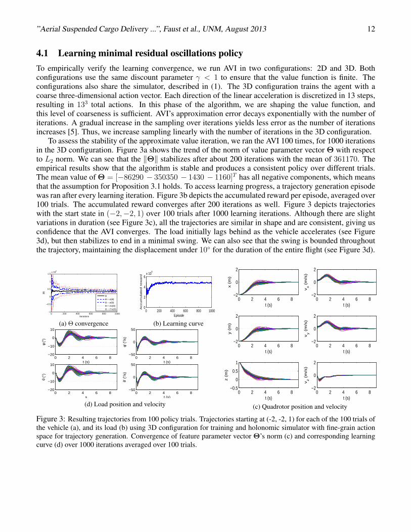
4.1 Learning minimal residual oscillations policyTo empirically verify the learning convergence, we run AVI in two configurations: 2D and 3D. Bothconfigurations use the same discount parameter γ < 1 to ensure that the value function is finite. Theconfigurations also share the simulator, described in (1). The 3D configuration trains the agent with acoarse three-dimensional action vector. Each direction of the linear acceleration is discretized in 13 steps,resulting in 133 total actions. In this phase of the algorithm, we are shaping the value function, andthis level of coarseness is sufficient. AVI’s approximation error decays exponentially with the number ofiterations. A gradual increase in the sampling over iterations yields less error as the number of iterationsincreases [5]. Thus, we increase sampling linearly with the number of iterations in the 3D configuration.

To assess the stability of the approximate value iteration, we ran the AVI 100 times, for 1000 iterationsin the 3D configuration. Figure 3a shows the trend of the norm of value parameter vector Θ with respectto L2 norm. We can see that the ‖Θ‖ stabilizes after about 200 iterations with the mean of 361170. Theempirical results show that the algorithm is stable and produces a consistent policy over different trials.The mean value of Θ = [−86290 − 350350 − 1430 − 1160]T has all negative components, which meansthat the assumption for Proposition 3.1 holds. To access learning progress, a trajectory generation episodewas ran after every learning iteration. Figure 3b depicts the accumulated reward per episode, averaged over100 trials. The accumulated reward converges after 200 iterations as well. Figure 3 depicts trajectorieswith the start state in (−2,−2, 1) over 100 trials after 1000 learning iterations. Although there are slightvariations in duration (see Figure 3c), all the trajectories are similar in shape and are consistent, giving usconfidence that the AVI converges. The load initially lags behind as the vehicle accelerates (see Figure3d), but then stabilizes to end in a minimal swing. We can also see that the swing is bounded throughoutthe trajectory, maintaining the displacement under 10◦ for the duration of the entire flight (see Figure 3d).

0 200 400 600 800 1000−1

−0.5

0

0.5

1

1.5x 10

6

Iterations

|Θ|

ΘΘ + σ(Θ)

Θ − σ(Θ)

Θ + 2σ(Θ)

Θ − 2*σ(Θ)

(a) Θ convergence

0 200 400 600 800 10000

2

4

6x 10

6

Episode

Accu

mu

late

d r

ew

ard

(b) Learning curve

0 2 4 6 8−2

0

2Position

t (s)

x (

m)

0 2 4 6 8−2

0

2

t (s)

y (

m)

0 2 4 6 8−0.5

0

0.5

1

t (s)

z (

m)

0 2 4 6 8−2

0

2Linear Velocity

t (s)v

x (

m/s

)

0 2 4 6 8−2

0

2

t (s)

vy (

m/s

)

0 2 4 6 8−2

0

2

t (s)

vz (

m/s

)

(c) Quadrotor position and velocity

0 2 4 6 8−20

−10

0

10

t (s)

φ (°

)

Angular position over time

0 2 4 6 8−20

−10

0

10

s

θ (°

)

0 2 4 6 8−50

0

50

t (s)

φ’ (°

/s)

Angular speed over time

0 2 4 6 8−50

0

50

θ’ (°

/s)

t (s)

(d) Load position and velocity

Figure 3: Resulting trajectories from 100 policy trials. Trajectories starting at (-2, -2, 1) for each of the 100 trials ofthe vehicle (a), and its load (b) using 3D configuration for training and holonomic simulator with fine-grain actionspace for trajectory generation. Convergence of feature parameter vector Θ’s norm (c) and corresponding learningcurve (d) over 1000 iterations averaged over 100 trials.


4.2 Minimal residual oscillations trajectory generationIn this section we evaluate effectiveness of the learned policy. We show the policy’s viability in theexpanded state and action spaces in simulation in Section 4.2.1. Section 4.2.2 assess the discrepancybetween the load displacement predictions in simulation and encountered experimentally during the flight.The section also compares experimentally the trajectory created using the learned policy to two othermethods: a cubic spline trajectory, which is a C3-class trajectory without any pre-assumptions about theload swing, and, to a dynamic programming trajectory [20], an optimal trajectory for a fixed start positionwith respect to its MDP setup.

4.2.1 State and action space expansion

We assess the quality and robustness of a trained agent in simulation by generating trajectories fromdifferent distances for two different simulators. The first simulator is a generic holonomic aerial vehiclewith a suspended load simulator, the same simulator we used in the learning phase. The second simulatoris a stochastic holonomic aerial vehicle with suspended simulator that adds up to 5% uniform noise tothe predicted state. Its intent is to simulate the inaccuracies and uncertainties of the physical hardwaremotion. We compare the performance of our learned, generated trajectories with model-based dynamicprogramming (DP) and cubic trajectories. The cubic and DP trajectories are generated using methodsdescribed in [20], but instead of relying on the full quadrotor-load system, we use the simplified modelgiven by (1). The cubic and DP trajectories are of the same duration as corresponding learned trajectories.The agent is trained in 3D configuration. For trajectory generation, we use a fine-grain, discretized 3Daction space A = (−3 : 0.05 : 3)3. This action space is ten times per dimension finer, and contains 1213different actions. The trajectories were generated at 50Hz with a maximum duration of 15 seconds. Alltrajectories were generated and averaged over 100 trials. To assess how well a policy adapts to differentstarting positions, we choose two different fixed positions, (-2,-2, 1) and (-20,-20,15), and two variablepositions. The variable positions are randomly drawn from between 4 and 5 meters, and within 1 meterfrom the goal state. The last position measures how well the agent performs within the sampling box. Therest of the positions are well outside of the sampling space used for the policy generation, and assess howwell the method works for trajectories outside of the sampling bounds with an extended state space.

Table 1 presents the averaged results with their standard deviations. We measure the end state andthe time when the agent reaches the goal, the percentage of trajectories that reach the goal state within15 seconds, and the maximum swing experienced among all 100 trials. With the exception of the noisyholonomic simulator at the starting position (-20,-20,15), all experiments complete the trajectory within4 cm of the goal, and with a swing of less than 0.6◦, as Proposition 3.1 predicts. The trajectories usingthe noisy simulator from a distance of 32 meters (-20,-20,15) don’t reach within 5 cm because 11% of thetrajectories exceed the 15-second time limit before the agent reaches its destination. However, we still seethat the swing is reduced and minimal at the destination approach, even in that case. The results show thattrajectories generated with stochastic simulator on average take 5% longer to reach the goal state, and thestandard deviations associated with the results is larger. This is expected, given the random nature of thenoise. However, all of the stochastic trajectories approach the goal with about the same accuracy as thedeterministic trajectories. This finding matches our prediction from Section 3.2.

The maximum angle of the load during its entire trajectory for all 100 trials depends on the inversedistance from the initial state to the goal state. For short trajectories within the sampling box, the swingalways remains within 4◦, while for very long trajectories it could go up to 46◦. As seen in Figure 3, thepeak angle is reached at the beginning of the trajectory during the initial acceleration, and as the trajectoryproceeds, the swing reduces. This makes sense, given that the agent is minimizing the combination of theswing and distance. When very far away from the goal, the agent will move quickly toward the goal stateand produce increased swing. Once the agent is closer to the goal state, the swing component becomesdominant in the value function, and the swing reduces.


Figure 4 shows the comparison of the trajectories with the same starting position (-2, -2, 1) and thesame Θ parameter, generated using the models above (AVI trajectories) compared to cubic and DP trajec-tories. First, we see that the AVI trajectories share a similar velocity profile (Figure 4a) with two velocitypeaks, both occurring in the first half of the flight. Velocities in DP and cubic trajectories have a singlemaximum in the second half of the trajectory. The resulting swing predictions (Figure 4b) shows that inthe last 0.3 seconds of the trajectory, the cubic trajectory exhibits a swing of 10◦, while the DP trajectoryends with a swing of less than 5◦. The AVI generated trajectories produce load displacement within 2◦

in the same time period. To assess energy of the load’s motion and compare different trajectories in thatway, Figure 4 shows one-sided power spectral density of the load displacement angles. We see that theenergy per frequency of the cubic trajectory is above the other three trajectories. Inspecting the averageenergy of AVI holonomic (E([φ θ]) = [0.0074 0.0073]) , noisy AVI (E([φ θ]) = [0.0050 0.0050]), andDP trajectories (E([φ θ]) = [0.0081 0.0081) load position signals, we find that AVI holonomic trajectoryrequires the least amount of energy over the entire trajectory.

0 1 2 3−2

−1

0Position

t (s)

x (m

)

0 1 2 3−2

−1

0

t (s)

y (m

)

0 1 2 30

0.5

1

1.5

t (s)

z (m

)

0 1 2 3−1

0

1

Linear Velocity

t (s)

v x (m

/s)

0 1 2 3−1

0

1

t (s)

v y (m

/s)

0 1 2 3−1

0

1

t (s)

v z (m

/s)

AVI holonomicAVI noisyDynamic programmingCubic

(a) Quadrotor position and velocity

0 1 2 3−10

−5

0

5

10Angular Position over Time

t (s)

φ (°)

0 1 2 3−10

−5

0

5

10

t (s)

θ (°)

0 1 2 3−50

0

50Angular Speed over Time

t (s)

φ (°/

s)

0 1 2 3−50

0

50

t (s)

θ (°/

s)

Linear Velocity


(b) Load position and velocity

0 2 4 6 8 10 12−90

−80

−70

−60

−50

−40

−30

−20

−10

Frequency (Hz)

θ P

ower

/freq

uenc

y (d

B/H

z)


0 2 4 6 8 10 12−100

−80

−60

−40

−20

0

Frequency (Hz)

θ P

ower

/freq

uenc

y (d

B/H

z)


(c) Power spectral density

Figure 4: AVI trajectory comparison to DP and cubic trajectories in simulation. Trajectories of the (a) vehicle, (b) itsload, and (c) load displacement’s power spectral density where the training was performed in 3D configuration, andthe trajectories were generated using generic and noisy holonomic simulators compared to the cubic and dynamicprogramming trajectories of the same duration.

4.2.2 Experimental results

We first trained an agent in 2D configuration. The 2D configuration uses a finer discretization of the actionspace, although only in the x and y directions. There are 121 actions in each direction, totaling to 1212

actions in the discretized space. This configuration uses a fixed sampling methodology. [5] show that theapproximation error stabilizes to a roughly constant level after the parameters stabilize. Once the agentwas trained, we generated trajectories for two experiments: constant altitude flight and flight with changingaltitude. To generate trajectories, we used a fine-grain, discretized 3D action space A = (−3 : 0.05 : 3)3.Trajectories were generated at 50Hz using the generic holonomic aerial vehicle carrying a suspended loadsimulator, the same simulator that was used in the learning phase. These trajectories were sent to thequadrotor with a suspended load weighing 45 grams on a 62 cm-long suspension cable.

In the constant altitude flight, the quadrotor flew from (-1,-1,1) to (1,1,1). Figure 5 compares the vehi-cle and load trajectories for a learned trajectory as flown and in simulation, with cubic and DP trajectories


Table 1: Summary of AVI trajectory results for different starting position averaged over 100 trials: percent com-pleted trajectories within 15 seconds, time to reach the goal, final distance to goal, final swing, and maximum swing.

State Goal reached t (s) ‖ p ‖ (m) ‖ η ‖ (◦) max ‖ η ‖ (◦)Location Simulator (%) µ σ µ σ µ σ µ σ

(-2,-2,1)Deterministic 100 6.13 0.82 0.03 0.01 0.54 0.28 12.19 1.16Stochastic 100 6.39 0.98 0.04 0.01 0.55 0.30 12.66 1.89

(-20,-20,15)Deterministic 99 10.94 1.15 0.04 0.01 0.49 0.33 46.28 3.90Stochastic 89 12.04 1.91 0.08 0.22 0.47 0.45 44.39 7.22

((4,5),(4,5),(4,5))Deterministic 100 7.89 0.87 0.04 0.01 0.36 0.31 26.51 2.84Stochastic 100 7.96 1.11 0.04 0.01 0.44 0.29 27.70 3.94

((-1,1),(-1,1),(-1,1))Deterministic 100 4.55 0.89 0.04 0.01 0.33 0.30 3.36 1.39Stochastic 100 4.55 1.03 0.04 0.01 0.38 0.29 3.46 1.52

0 1 2 3 4 5

−1

0

1

Position

t (s)

x (

m)

0 1 2 3 4 5

−1

0

1

t (s)

y (

m)

0 1 2 3 4 50.5

1

1.5

t (s)

z (

m)

LearnedCubicDPSimulation

(a) Quadrotor position

0 1 2 3 4 5−15

−10

−5

0

5

10

15Angular position of the load

t(s)

φ(°

)

0 1 2 3 4 5−15

−10

−5

0

5

10

15

t (s)

θ (

°)


(b) Load position

0 10 20 30 40 50−120

−100

−80

−60

−40

−20

0

Frequency (Hz)

φ Pow

er/fr

eque

ncy

(dB/

Hz)


0 10 20 30 40 50−120

−100

−80

−60

−40

−20

0

Frequency (Hz)

θ Pow

er/fr

eque

ncy

(dB/

Hz)



Figure 5: AVI experimental trajectories. Quadrotor (a), load (b) trajectories, and power spectral density (c) as flown,created through learning compared to cubic, dynamic programming, and simulated trajectories.


0 0.5 1 1.5 2 2.5 3 3.5 4 4.5−1

0

1Quadrotor Position

t (s)

x (

m)

0 0.5 1 1.5 2 2.5 3 3.5 4 4.5−1

0

1

t (s)

y (

m)

0 0.5 1 1.5 2 2.5 3 3.5 4 4.50

2

4

t (s)

z (

m)

Trail 1Trail 2Trail 3Simulation


0 0.5 1 1.5 2 2.5 3 3.5 4 4.5−10

−505

10

t (s)

φ (

° )

0 0.5 1 1.5 2 2.5 3 3.5 4 4.5−10

−505

10

t (s)

θ (

° )

Trial 1Trail 2Trail 3Simulation

(b) Load position

0 5 10 15 20 25−100

−80

−60

−40

−20

0

Frequency (Hz)

φ Pow

er/fre

quen

cy (d

B/Hz

)

Trial 1Trail 2Trial 3Simulation

0 5 10 15 20 25−100

−80

−60

−40

−20

0

Frequency (Hz)

θ Pow

er/fre

quen

cy (d

B/Hz

)

Trial 1Trail 2Trial 3Simulation


Figure 6: AVI experimental results of altitude changing flight. Quadrotor (a), load (b) trajectories, and powerspectral density (c) as flown and in simulation, over three trials in the altitude changing test trained in planar actionspace.

of the same length and duration. The vehicle trajectories in Figure 5a suggest a difference in the velocityprofile, with the learned trajectory producing a slightly steeper acceleration between 1 and 2.5 seconds.The learned trajectory also contains a 10 cm vertical move up toward the end of the flight. To compare theflown trajectory with the simulated trajectory, we look at the load trajectories in Figure 5b. We notice thereduced swing, especially in the second half of the load’s φ coordinate. The trajectory in simulation neverexceeds 10◦, and the actual flown trajectory reaches its maximum at 12◦. Both learned load trajectoriesfollow the same profile with three distinct peaks around 0.5 seconds, 2.2 seconds, and 3.1 seconds intothe flight, followed by rapid swing control and reduction to under 5◦. The actual flown trajectory natu-rally contains more oscillations that the simulator didn’t model. Despite that, the limits, boundaries, andprofiles of the load trajectories are close between the simulation and flown trajectories. This verifies thevalidity of the simulation results: the load trajectory predictions in the simulator are reasonably accurate.Comparing the flown learned trajectory with a cubic trajectory, we see a different swing profile. The cubicload trajectory has higher oscillation, four peaks within 3.5 seconds of flight, compared to three peaks forthe learned trajectory. The maximum peak of the cubic trajectory is 14

◦ at the beginning of the flight.The most notable difference happens after the destination is reached during the hover (after 3.5 secondsin Figure 5b. In this part of the trajectory, the cubic trajectory shows a load swing of 5 − 12◦, while thelearned trajectory controls the swing to under 4◦. Figure 5b shows that the load of the trajectory learnedwith reinforcement learning stays within the load trajectory generated using dynamic programming at alltimes: during the flight (the first 3.4 seconds) and the residual oscillation after the flight. Power spectraldensity in Figure 5a shows that, during experiments, learned trajectory contains less energy per frequencythan cubic and DP trajectories.

In the second set of experiments, the same agent was used to generate changing altitude trajectoriesthat demonstrate ability to expand action space between learning and planning. Note that the trajectoriesgenerated for this experiment used value approximator parameters learned on a 2D action space, in thexy-plane, and produced a viable trajectory that changes altitude because the trajectory generation phaseused 3D action space. This property was predicted by Proposition 3.1 since the extended 3D action spaceallows transitions to the higher value states. The experiment was performed three times and the resultingquadrotor and load trajectories are depicted in Figure 6. The trajectories are consistent between three trialsand follow closely simulated trajectory (Figure 6a). The load displacement (Figure 6b) remains under 10◦and exhibits minimal residual oscillations. Figure 6c shows that the energy profile between the trialsremains consistent.


4.3 Swing-free path trackingPath tracking with reduced load displacement evaluation compares the load displacement and trackingerrors of the Algorithm 1 with two other methods: a minimal residual oscillations method describedin Section 3.2, and path tracking with no load displacement reduction. The path tracking-only methodchooses actions that transition the system as close as possible to the tracking trajectory in the directionof the goal state with no consideration to the load swing. We use three reference trajectories: a straightline, a two-line segment, and a helix. To generate the trajectory, we use action space discretized in 0.1equidistant steps, and the same value function parametrization, Θ, used in the evaluations in Section 4.2and learned in Section 3.1.

Table 2: Summary of path tracking results for different trajectory geometries: reference path, m, proximity factor(δ), trajectory duration, maximum swing, and maximum deviation from the reference path (error). Best results forreference path are highlighted.

Ref. path m δ (m) t (s) ‖η‖ (◦) Error (m)

Line

100 0.01 11.02 21.94 0.02500 0.01 11.02 20.30 0.03100 0.05 6.64 23.21 0.08500 0.05 7.06 23.22 0.11

Tracking only 100 0.01 11.02 73.54 0.01Minimal residual oscillations - - 6.74 18.20 0.49

Multi-segment line

100 0.01 7.52 20.17 0.04500 0.01 7.52 23.11 0.50100 0.05 7.52 28.24 0.10500 0.05 7.52 26.70 0.88


Helix

100 0.01 5.72 29.86 0.39500 0.01 5.72 26.11 0.44100 0.05 5.76 32.13 0.17500 0.05 5.72 22.20 0.11


Table 2 examines the role of the proximity parameter δ, and candidate actions set size parameterm. Recall that the Algorithm 1 used δ as a distance from the reference trajectory where all actions thattransition the system within δ distance will be considered for load swing reduction. If there were nosuch actions, then the algorithm selects m actions that transition the system the closest to the referencetrajectory, regardless of the actual physical distance. We look at two proximity factors and two action setsize parameters. In all cases, the proposed method, swing-free path tracking, exhibits smaller path trackingerror than minimal residual oscillations method, and smaller load displacement results than tracking-onlymethod. Also for each reference path, there is a set of parameters that provides good balance betweentracking error and load displacement reduction.

Figure 7 presents results of the tracking and load displacement errors for the same three referencepaths: line, multi-segment, and helix. We compare them to tracking-only and minimal residual oscillationsAVI algorithms. Figure 7a displays the trajectories. We see that in all three cases, the minimal residualoscillations algorithm took a significantly different path from the other two. Its goal was to minimize thedistance to the goal state as soon as possible while reducing the swing, and it does not follow the reference


−1

0

1

2

3

−101234

0

0.5

1

1.5

2

yx

z

Path tracking onlyMinimal res. oscillations onlyReduced swing w/ path trackingReference path

−2

0

2

4

−101234

−2

0

2

4

6

yx

z


−1

0

1

2

−2−1.5−1−0.500.5

−2

0

2

4

6

yx

z


(a) Trajectory

0 1 2 3 4 510

−8

10−6

10−4

10−2

100

Trajectory (m)

Accu

mu

late

d S

qu

are

d E

rro

r (m

2)

Path tracking onlyMinimal res. oscillations onlyReduced swing w/ path tracking

0 1 2 3 4 5 6 7 8 910

−8

10−6

10−4

10−2

100

102

Trajectory (m)

Accu

mu

late

d S

qu

are

d E

rro

r (m

2)


0 1 2 3 4 5 6 710

−8

10−6

10−4

10−2

100

102

Trajectory (m)

Accu

mu

late

d S

qu

are

d E

rro

r (m

2)


(b) Line tracking error

0 10 20 30 40 50−100

−80

−60

−40

−20

0

20

Frequency (Hz)

φ P

ow

er/

fre

qu

en

cy (

dB

/Hz)


0 10 20 30 40 50−100

−80

−60

−40

−20

0

20

Frequency (Hz)

θ P

ow

er/

fre

qu

en

cy (

dB

/Hz)


0 10 20 30 40 50−120

−100

−80

−60

−40

−20

0

Frequency (Hz)

φ P

ow

er/

fre

qu

en

cy (

dB

/Hz)


0 10 20 30 40 50−120

−100

−80

−60

−40

−20

0

Frequency (Hz)

θ P

ow

er/

fre

qu

en

cy (

dB

/Hz)


0 10 20 30 40 50−150

−100

−50

0

50

Frequency (Hz)

φ P

ow

er/

fre

qu

en

cy (

dB

/Hz)


0 10 20 30 40 50−120

−100

−80

−60

−40

−20

0

Frequency (Hz)

θ P

ow

er/

fre

qu

en

cy (

dB

/Hz)



Figure 7: Swing-free path tracking for line, multi-segment, and helix reference trajectories, compared to pathtracking only, and to load displacement control only (a). Tracking error (b) is in logarithmic scale, and powerspectral density (c).

path. Figure 7b quantifies the accumulated tracking error. Path tracking error for Algorithm 1 remainsclose to the tracking-only trajectory. For all three trajectories, the accumulated tracking error is one totwo orders of magnitude smaller than for the minimal residual oscillations method. Examining the loaddisplacement characteristics though power spectral analysis of the vector η = [φ θ]T time series, we noticethat frequency profile of the trajectory generated with Algorithm 1 resembles closely that of the minimalresidual oscillations trajectory (Figure 7c). In contrast, power spectral density of tracking only trajectoriescontain high frequencies absent in the trajectories created with the other two methods. Thus, the proposedmethod for swing-free path tracking, with its tracking error characteristics similar to the tracking-onlymethod, and its load displacement characteristics similar to the minimal residual oscillations method,offers a solid compromise between the two extremes.

4.4 Automated aerial cargo deliveryIn this section we evaluate the methods for an aerial cargo delivery task developed in 3.5. Our goal is toverify that the method finds collision-free paths and creates trajectories that closely follow the paths whilenot exceeding the given maximal load displacement. The method’s performance in simulation is discussedin Section 4.4.1, and its experimental evaluation, in Section 4.4.2.

The simulations and experiments were performed using the same setup as for minimal residual oscil-lations tasks in obstacle-free environments, described in Section 4.2. In our PRM set up, we use uniformrandom sampling. Each node in the roadmap is connected to its 10 nearest neighbors using Euclidean dis-tance. A straight line planner with a resolution of 5 cm creates the edges in the graph. The path planningwas done using the Parasol Motion Planning Library from Texas A&M University [22].


(a) Cafe (b) Testbed Environment 1 (c) Testbed Environment 2

Figure 8: Benchmark environments studied in simulation (a) and experimentally (b-c)

4.4.1 Trajectory planning in Cafe

To explore conceptual applications of the quadrotors to domestic and assistive robotics and to test themethod in a more challenging environment, we choose a virtual coffee shop setting for our simulationtesting. In this setting, the cargo delivery tasks (Problem 2.2) include: delivering coffee, delivering checksto the counter, and fetching items from high shelves (see Figure 8a). The UAV needs to pass a doorway,change altitude, and navigate between the tables, shelves, and counters. In all these tasks, both speed andload displacement are important factors. We want the service to be in a timely manner, but it is importantthat the swing of the coffee cup, which represents the load, is minimized so that the drink is not spilled.The Cafe is 30 meters long, 10 meters wide, and 5 meters tall.

We generate the paths, and create trajectories for three different maximal load displacements (1◦, 10◦,and 25◦). Since the path planning is the most complex for the largest bounding volume, and the same pathcan be reused for smaller maximal load displacements, we create the path once using the bounding volumewith a 25◦ cone half aperture, and create trajectories along the path requiring the same or lower maximalload displacement. The proximity factor is δ = 5 cm and the candidate action sets size is m = 500.We evaluate the number of added waypoints to meet the load displacement requirement, the trajectoryduration, the maximum swing, and the maximum path-tracking error.

Table 3 summarizes the results of the trajectory characteristics for the three tasks in the coffee shop fordifferent maximal load displacement. It demonstrates that we can control load and follow the path to anarbitrary small load displacement. The maximum swing along a trajectory always stays under the requiredload displacement bound. The tracking error stays within 10 cm, regardless of the path and decreases as themaximal load displacement bound decreases. Therefore, by designing the bounding volume with 10 cm ofclearance, the quadrotor-load system will not collide with the environment. The delivery time and numberof added waypoints increase with the decrease of the required load displacement bound, as expected.Although, it is common sense that slower trajectories produce less swing, the agent automatically chooseswaypoints so not to needlessly slow down the trajectories.

Figure 9 depicts the trajectory of the quadrotor and the load during the coffee delivery task for requiredmaximal load displacements of 1◦, 10◦, and 25◦. The trajectories are smooth, and the load’s residual oscil-lations are minimal in all of them. The trajectory and path overlay is presented in Figure 10. The numberof inserted waypoints increases for the smaller angles. The tracking error over the trajectory length is dis-played in Figure 10d. The accumulated squared error profiles differ based on the load displacement anglebound, with the 1◦ trajectory having accumulated error significantly smaller than other two trajectories.

4.4.2 Experimental evaluation

The goals of the experiments are to show the discrepancy between the simulation results and the observedexperimental trajectories, and to demonstrate the safety and feasibility of the method by using a quadrotorto deliver a cup of water. To check the discrepancy between the simulation predictions of the maximum


Table 3: Summary of path and trajectory results for different tasks in the Cafe setting: task name and maximumallowed load displacement (‖η‖), obstacle-free path length, and number of waypoints, trajectory waypoints afterbisection, trajectory durations (t), maximum swing (‖η‖), and maximum deviation from the path (error).

Task Path TrajectoryName ‖η‖ (◦) Length (m) Pts. Pts. t (s) ‖η‖ (◦) Error (m)Deliver coffee 25 23.20 3 7 43.02 24.60 0.08

10 23.20 3 17 67.18 9.34 0.061 23.20 3 97 258.62 0.86 0.03

Pay 25 15.21 1 3 25.98 18.23 0.0610 15.21 1 7 28.64 8.94 0.051 15.21 1 63 172.28 0.92 0.01

Special 25 32.57 1 7 52.54 24.11 0.07request 10 32.57 1 22 82.76 9.58 0.05

1 32.57 1 128 349.86 0.92 0.01

0 100 200−10

0

10

t (s)

x (

m)

0 100 200−10

0

10

t (s)

y (

m)

0 100 2000

2

4

t (s)

z (

m)

0 100 200−2

0

2

t (s)

vx (

m/s

)

0 100 200−2

0

2

t (s)

vy (

m/s

)

0 100 200−2

0

2

t (s)

vz (

m/s

)

0 100 200−20

0

20

t (s)

φ (°

)

0 100 200−20

0

20

t (s)

θ (°

)

0 100 200−100

0

100

t (s)

v φ°/s

0 100 200−100

0

100

t (s)

v θ (°/

s)

(a) σ = 1◦

0 20 40 60−10

0

10

t (s)

x (

m)

0 20 40 60−10

0

10

t (s)

y (

m)

0 20 40 600

2

4

t (s)

z (

m)

0 20 40 60−2

0

2

t (s)

vx (

m/s

)

0 20 40 60−2

0

2

t (s)

vy (

m/s

)

0 20 40 60−2

0

2

t (s)

vz (

m/s

)

0 20 40 60−20

0

20

t (s)

φ (°

)

0 20 40 60−20

0

20

t (s)

θ (°

)

0 20 40 60−100

0

100

t (s)

v φ°/s

0 20 40 60−100

0

100

t (s)

v θ (°/

s)

(b) σ = 10◦

0 20 40−10

0

10

t (s)

x (

m)

0 20 40−10

0

10

t (s)

y (

m)

0 20 400

2

4

t (s)z (

m)

0 20 40 60−2

0

2

t (s)

vx (

m/s

)

0 20 40 60−2

0

2

t (s)

vy (

m/s

)

0 20 40 60−2

0

2

t (s)

vz (

m/s

)

0 20 40 60−20

−10

0

10

20

s

φ (°)

Angular position over time

0 20 40 60−20

−10

0

10

20

s

θ (°)

0 20 40 60−100

−50

0

50

100

s

°/s

Angular speed over time

0 20 40 60

−50

0

50

°/s

(c) σ = 25◦

Figure 9: Quadrotor and load trajectories in coffee delivery task in the Cafe for maximal allowed load displacementof 1◦, 10◦, and 25◦. Zero altitude is the lowest point that a cargo equipped quadrotor can fly without the loadtouching the ground.

load displacement in simulation and experimentally, we run queries in two testbed environments to gen-erate trajectories in simulation. The testbed environments are all 2.5 meters by 3 meters, with the ceilingheight varying from 1.5 meters to 2.5 meters. The obstacles are uniform triangular prisms with 60 cmsides. Shorter obstacles are 60 cm tall, while the tall ones are 1.2 meters tall. They differ in numberof obstacles, their sizes, and locations. The first testbed environment contains three obstacles positioneddiagonally across the room and the same landing platform (see Figure 8b). Two obstacles are 0.6 meterstall, while the third one is 1.2 meters tall. The second testbed environment is filled with five 1.2 meterstall obstacles. They are in the corners and in the middle of a 2.5 by 2 meters rectangle centered in theroom (Figure 8c). This is a challenging, cluttered space that allows us to experimentally test an urbanenvironment setting.


−50

510

−5

0

5

100

1

2

3

xy

z

TrajectoryReference

(a) 25◦−5

05

10

−5

0

5

100

1

2

3

xy

z

TrajectoryReference

(b) 10◦−5

05

10

−50

510

0

1

2

3

xy

z

TrajectoryReference

(c) 1◦0 5 10 15 20

0

0.005

0.01

0.015

0.02

0.025

0.03

0.035

Trajectory (m)

Acc

umul

ated

Squ

ared

Err

or (

m2 )

25°

10°

1°

(d) Tracking error

Figure 10: Path bisecting for Deliver coffee task based on the maximum allowed load displacement (a-c). Accu-mulated squared tracking error along the trajectory for different maximum allowed load displacements (d).

Table 4: Summary of path and simulated and experimental trajectory characteristics for different obstacle config-urations:task name and maximum allowed load displacement (η); obstacle-free path length (l), and its number ofwaypoints (#); simulated trajectory: waypoints after bisection (#), planned trajectory durations (t), maximum swing(η), and maximum deviation from the path (error); experimental trajectory: maximum swing (η) and maximumdeviation from the path (error). The experimental results are average over three trials.

Task Path Simulation ExperimentTest. ‖η‖ (◦) l (m) # # t (s) ‖η‖ (◦) Error (m) ‖η‖ (◦) Error (m)Env. 1 10 3.86 3 3 12.64 7.25 0.05 11.32 0.16

5 3.86 3 4 15.68 3.63 0.03 7.99 0.111 3.86 3 16 44.98 0.98 0.04 5.05 0.07

Env. 2 10 3.23 2 2 10.18 5.51 0.05 9.94 0.165 3.23 2 4 15.80 2.66 0.05 6.72 0.111 3.23 2 16 42.24 0.69 0.02 4.98 0.07

Table 4 summarizes the difference in observed versus predicted maximum load displacement for thesetasks over three trials. The observed maximum displacement is between 4◦ an 5◦ higher experimentallythan in simulation. This is expected and due to unmodeled system dynamics, noise, wind influence andother factors and it matches load displacement observed during hover.

Figure 11 shows three trials of the experimentally flown trajectory in Environment 2 (Figure 8c), withthe predicted simulation. The vehicle trajectory matches very closely between trials and the simulation.The load’s trajectories show higher uncertainty over the position of the load at any given time. However,the load displacement is bounded and stays within 10◦.

The demonstration of the practical feasibility and safety of this method was demonstrated by usingthe system to deliver a cup of water to a static human subject. In this demonstration, the quadrotor’s loadis a 250 ml paper cup filled with 100 ml of water. In Environment 1 (see Figure 8b), a quadrotor needsto fly diagonally through the room, avoiding a set of three obstacles. The path and trajectory used forthis demonstration are the same referenced in Table 4. A human subject was seated at the table. As thequadrotor competed the flight, it set the cup of water in front of the human, who detached it from thequadrotor. A video of the human-quadrotor interaction can be found in the enclosed video submission.

5 ConclusionIn this work we proposed an autonomous aerial cargo delivery agent that works in environments with staticobstacles to plan and create trajectories with bounded load displacements. At the heart of the method is thereinforcement learning policy for minimal residual oscillations trajectories. This article showcases how a


0 2 4 6 8 10−2

0

2

t (s)

x (

m)

0 2 4 6 8 10−2

0

2

t (s)

y (

m)

0 2 4 6 8 100.5

1

1.5

t (s)

z (

m)

Trial 1Trial 2Trail 3Simulation


0 2 4 6 8 10−10

−505

10

t(s)

φ(de

gree

s)

0 2 4 6 8 10−10

−505

10

t (s)

θ (d

egre

es)

Trial 1Trial 2Trial 3Simulation

(b) Load position 0 10 20 30 40 50−150

−100

−50

0

Frequency (Hz)

φ P

ow

er/

fre

qu

en

cy (

dB

/Hz)

Trail 1Trial 2Trail 3Simulation

0 10 20 30 40 50−150

−100

−50

0

Frequency (Hz)

θ p

hi P

ow

er/

fre

qu

en

cy (

dB

/Hz)

Trail 1Trail 2Trail 3Simulation


0 2 4 6 8 100

0.05

0.1

t (s)A

ccum

ula

ted e

rror

(m2)

Trial 1Trial 2Trial 3Simulation

(d) Accumulated tracking error

Figure 11: Experimental quadrotor (a) and load (b) trajectories, power spectral density (c), and accumulated pathtracking error (d) in the second testbed configuration.

reinforcement learning policy learned through a single training can be adapted to perform different tasksand impose nonholonomic constraints on the system. We modified the policy by restricting the domain’saction space to track a reference path with a bounded load displacement. Finally, we integrated the swing-free path tracking and sampling-based path planning to solve the aerial cargo delivery task. We evaluatedeach of the modules separately, and showed that learning converges to a single policy, and that performsminimal residual oscillation delivery task, that the policy is viable with expending state and action spaces.The simulations quality is assessed through the comparison with experimental load displacement on aphysical robot. Then we evaluated the swing-free path tracking on three reference paths for varyingvalues of the tacking parameters. The results demonstrated that the proposed method attains both goodtracking and good load displacement characteristics. Lastly, results of the integration with sampling-basedmotion planning shows that the method creates collision-free trajectories with bound load displacementfor arbitrarily small load displacement bounds. We experimentally demonstrated the feasibility and safetyof the method by having a quadrotor deliver a cup of water to a human subject.

This article lays a foundation for aerial cargo delivery in environments with static obstacles. In fur-ther work, trajectory smoothing can be applied to the trajectories generated with this to speed them up.Moving obstacles can be handled through an online trajectory tracking that adapts to dynamical changesin environment.

6 AcknowledgmentsThe authors would like to thank Torin Adamson for creating virtual models of the Cafe, the testbed andthe UAV carrying the suspended load.

References[1] AscTec. Ascending Technologies GmbH, 2013. http://www.asctec.de/.

[2] R. E. Bellman. Dynamic Programming. Dover Publications, Incorporated, 1957.

[3] M. Bernard and K. Kondak. Generic slung load transportation system using small size helicopters. In Roboticsand Automation, 2009. ICRA ’09. IEEE International Conference on, pages 3258 –3264, may 2009.


[4] D. Ernst, M. Glavic, P. Geurts, and L. Wehenkel. Approximate value iteration in the reinforcement learningcontext. application to electrical power system control. International Journal of Emerging Electric PowerSystems, 3(1):1066.1–1066.37, 2005. Download from: http://www.bepress.com/ijeeps/vol3/iss1/art1066.

[5] A. M. Farahmand, R. Munos, and C. Szepesvari. Error propagation for approximate policy and value iteration.In Advances in Neural Information Processing Systems, 2010.

[6] A. Faust, I. Palunko, P. Cruz, R. Feirro, and L. Tapia. Learning swing-free trajectories for uavs with a suspendedload. In IEEE International Conference on Robotics and Automation (ICRA), Karlsruhe, Germany, pages4887–4894, May 2013.

[7] D. Hsu, J.-C. Latombe, and R. Motwani. Path planning in expansive configuration spaces. In ICRA, pages2719–2726, 1997.

[8] L. E. Kavraki, P. Svestka, J. C. Latombe, and M. H. Overmars. Probabilistic roadmaps for path planning inhigh-dimensional configuration spaces. IEEE Trans. Robot. Automat., 12(4):566–580, August 1996.

[9] J. Kuffner, J.J. and S. LaValle. Rrt-connect: An efficient approach to single-query path planning. In Roboticsand Automation, 2000. Proceedings. ICRA ’00. IEEE International Conference on, volume 2, pages 995 –1001vol.2, 2000.

[10] V. Kumar and N. Michael. Opportunities and challenges with autonomous micro aerial vehicles. The Interna-tional Journal of Robotics Research, 31(11):1279–1291, Sept. 2012.

[11] S. M. LaValle. Planning Algorithms. Cambridge University Press, Cambridge, U.K., 2006.

[12] S. M. Lavalle, J. J. Kuffner, and Jr. Rapidly-exploring random trees: Progress and prospects. In Algorithmicand Computational Robotics: New Directions, pages 293–308, 2000.

[13] S. Lupashin and R. DAndrea. Adaptive open-loop aerobatic maneuvers for quadrocopters. In World Congress,volume 18, pages 2600–2606, 2011.

[14] N. Malone, K. Manavi, J. Wood, and L. Tapia. Construction and use of roadmaps that incoroporate worksapcemodeling errors. In To appear IEEE International Conference on Intellignet Robots and Systems (IROS), Nov2013.

[15] K. Manavi, B. S. Wilson, and L. Tapia. Simulation and analysis of antibody aggregation on cell surfacesusing motion planning and graph analysis. In ACM Conference on Bioinformatics, Computational Biology andBiomedicine, October 2012.

[16] MARHES. Multi-agent, robotics, hybrid, and embedded systems laboratory, department of copmuter andelectrical engineering, university of new mexico. http://marhes.ece.unm.edu, February 2013.

[17] H. B. McMahan, M. Likhachev, and G. J. Gordon. Bounded real-time dynamic programming: Rtdp withmonotone upper bounds and performance guarantees. In In ICML05, pages 569–576, 2005.

[18] D. Mellinger, N. Michael, and V. Kumar. Trajectory generation and control for precise aggressive maneuverswith quadrotors. The International Journal of Robotics Research, 31(5):664–674, 2012.

[19] N. Michael, D. Mellinger, Q. Lindsey, and V. Kumar. The grasp multiple micro-uav testbed. Robotics Automa-tion Magazine, IEEE, 17(3):56 –65, sept. 2010.

[20] I. Palunko, P. Cruz, and R. Fierro. Agile load transportation : Safe and efficient load manipulation with aerialrobots. Robotics Automation Magazine, IEEE, 19(3):69 –79, sept. 2012.

[21] I. Palunko, A. Faust, P. Cruz, L. Tapia, and R. Feirro. A reinforcement learning approach towards autonomoussuspended load manipulation using aerial robots. In IEEE International Conference on Robotics and Automa-tion (ICRA), Karlsruhe, Germany, pages 4881–4886, May 2013.


[22] Parasol. Parasol lab, department of computer science and engineering, texas a&m university.https://parasol.tamu.edu/, December 2012.

[23] A. P. Schoellig, F. L. Mueller, and R. DAndrea. Optimization-based iterative learning for precise quadrocoptertrajectory tracking. Autonomous Robots, 33:103–127, 2012.

[24] S. Shen, N. Michael, and V. Kumar. 3D estimation and control for autonomous flight with constrained compu-tation. In In Proc. IEEE Int. Conf. Robot. Autom. (ICRA),, Shanghai, China, may 2011. Submitted.

[25] A. A. Sherstov and P. Stone. Improving action selection in MDP’s via knowledge transfer. In Proceedings ofthe Twentieth National Conference on Artificial Intelligence, July 2005.

[26] K. Sreenath, N. Michael, and V. Kumar. Trajectory generation and control of a quadrotor with a cable-suspended load – a differentially-flat hybrid system. In IEEE International Conference on Robotics and Au-tomation (ICRA), pages 4873–4880, 2013.

[27] M. E. Taylor and P. Stone. Behavior transfer for value-function-based reinforcement learning. In F. Dignum,V. Dignum, S. Koenig, S. Kraus, M. P. Singh, and M. Wooldridge, editors, The Fourth International JointConference on Autonomous Agents and Multiagent Systems, pages 53–59, New York, NY, July 2005. ACMPress.

[28] Vicon. Vicon Motion Systems Limited, 2012. http://www.vicon.com/.

aerial suspended cargo delivery through reinforcement...

Documents