aeronautical voice radio channel modelling and simulation …€¦ · · 2006-05-11aeronautical...
TRANSCRIPT

Aeronautical Voice Radio Channel Modelling andSimulation ndash A Tutorial Review
Konrad Hofbauer12 and Gernot Kubin1
1 Graz University of TechnologySPSC ndash Signal Processing
and Speech Communication Laboratory8010 Graz Austria
konradhofbauertugrazatgernotkubintugrazat
2 Eurocontrol Experimental CentreINO ndash Innovative Research
91222 Breacutetigny-sur-Orge France
Abstractmdash The basic concepts in the modelling and simulationof the mobile radio channel are reviewed The time-variantchannel is dominated by multipath propagation Doppler effectpath loss and additive noise Stochastic reference models in theequivalent complex baseband facilitate a compact mathematicaldescription of the channelrsquos input-output relationship The realisa-tion of these reference models as filtered Gaussian processes leadsto practical implementations of frequency selective and frequencynonselective channel models
Three different small-scale area simulations of the aeronauticalvoice radio channel are presented We demonstrate the practicalimplementation of a frequency flat fading channel Based on ascenario in airground communication the parameters for thereadily available simulators are derived The resulting outputsgive insight into the characteristics of the channel and serve asa basis for the design of digital transmission and measurementtechniques
I INTRODUCTION
Air traffic control (ATC) has relied on the voice radio forcommunication between aircraft pilots and air traffic controloperators since its beginning The amplitude-modulation (AM)radio which is in operation worldwide has basically remainedunchanged for decades Given the aeronautical life cycleconstraints it is expected that the analogue radio will remainin use for ATC voice in Europe well beyond 2020 [1]
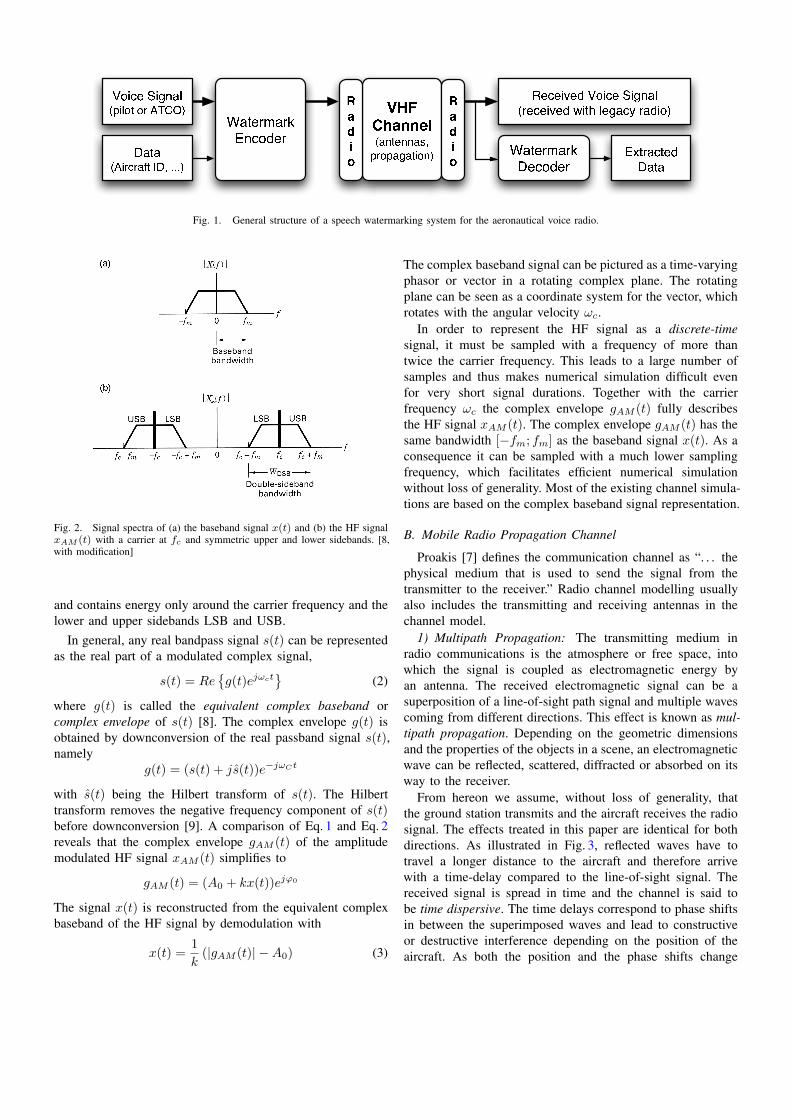
Eurocontrol Experimental Centre (France) and Graz Uni-versity of Technology (Austria) are currently working onembedding supplementary digital data such as the call-sign ofthe aircraft into the voice signal of the analogue airgroundcommunication (see [2] [3] and Fig 1) The radio trans-mission channel has a strong impact on the performance ofsuch a speech watermarking system in terms of data rate androbustness The degradation of the transmitted signal is studiedfor the purpose of system design and evaluation This paperreviews the general concepts of radio channel modelling anddemonstrates the use of simulators for the aeronautical voicechannel
Radio channel modelling has a long history and is a veryactive area of research This is especially the case with respectto terrestrial mobile radio communications and wide-band datacommunications due to commercial interest
However the results are not always transferable to the aero-nautical domain A comprehensive up-to-date literature review
on channel modelling and simulation with the aeronauticalradio in mind is provided in [4] It is highly recommended asa pointer for further reading and its content is not repeatedhere
II BASIC CONCEPTS
This and the following section are based on the work ofPaumltzold [5] and provide a summary of the basic characteristicsthe modelling and the simulation of the mobile radio channelAnother comprehensive treatment on this extensive topic isgiven in [6]
A Amplitude Modulation and Complex Baseband
The aeronautical voice radio is based on the double-sideband amplitude modulation (DSB-AM A3E or simplyAM) of a sinusoidal unsuppressed carrier [7] An analoguebaseband voice signal x(t) which is band-limited to a band-width fm modulates the amplitude of a sinusoidal carrier withamplitude A0 carrier frequency fc and initial phase ϕ0 Themodulated high frequency (HF) signal xAM (t) is defined as
xAM (t) = (A0 + kx(t)) cos(2πfct + ϕ0)
with the modulation depth
m =|kx(t)|max
A0le 1
The real-valued HF signal can be equivalently written usingcomplex notation and ωc = 2πfc as
xAM (t) = Re(A0 + kx(t))ejωctejϕ0
(1)
Under the assumption that fc fm the HF signal canbe demodulated and the input signal x(t) reconstructed bydetecting the envelope of the modulated sine wave Theabsolute value is low-pass filtered and the original amplitudeof the carrier is subtracted
x(t) =1k
([|xAM (t)|]LP minusA0)
Fig 2 shows the spectra of the baseband signal and thecorresponding HF signal Since the baseband signal is bydefinition low-pass filtered the HF signal is a bandpass signal
D a t a( A i r c r a f t I D )V o i c e S i g n a l( p i l o t o r A T C O ) W a t e r m a r kE n c o d e r V H FC h a n n e l( a n t e n n a s p r o p a g a t i o n ) R e c e i v e d V o i c e S i g n a l( r e c e i v e d w i t h l e g a c y r a d i o )W a t e r m a r kD e c o d e r E x t r a c t e dD a t aRad io Rad io
Fig 1 General structure of a speech watermarking system for the aeronautical voice radio
Fig 2 Signal spectra of (a) the baseband signal x(t) and (b) the HF signalxAM (t) with a carrier at fc and symmetric upper and lower sidebands [8with modification]
and contains energy only around the carrier frequency and thelower and upper sidebands LSB and USB
In general any real bandpass signal s(t) can be representedas the real part of a modulated complex signal
s(t) = Reg(t)ejωct
(2)
where g(t) is called the equivalent complex baseband orcomplex envelope of s(t) [8] The complex envelope g(t) isobtained by downconversion of the real passband signal s(t)namely
g(t) = (s(t) + js(t))eminusjωCt
with s(t) being the Hilbert transform of s(t) The Hilberttransform removes the negative frequency component of s(t)before downconversion [9] A comparison of Eq 1 and Eq 2reveals that the complex envelope gAM (t) of the amplitudemodulated HF signal xAM (t) simplifies to
gAM (t) = (A0 + kx(t))ejϕ0
The signal x(t) is reconstructed from the equivalent complexbaseband of the HF signal by demodulation with
x(t) =1k
(|gAM (t)| minusA0) (3)
The complex baseband signal can be pictured as a time-varyingphasor or vector in a rotating complex plane The rotatingplane can be seen as a coordinate system for the vector whichrotates with the angular velocity ωc
In order to represent the HF signal as a discrete-timesignal it must be sampled with a frequency of more thantwice the carrier frequency This leads to a large number ofsamples and thus makes numerical simulation difficult evenfor very short signal durations Together with the carrierfrequency ωc the complex envelope gAM (t) fully describesthe HF signal xAM (t) The complex envelope gAM (t) has thesame bandwidth [minusfm fm] as the baseband signal x(t) As aconsequence it can be sampled with a much lower samplingfrequency which facilitates efficient numerical simulationwithout loss of generality Most of the existing channel simula-tions are based on the complex baseband signal representation
B Mobile Radio Propagation Channel
Proakis [7] defines the communication channel as ldquo thephysical medium that is used to send the signal from thetransmitter to the receiverrdquo Radio channel modelling usuallyalso includes the transmitting and receiving antennas in thechannel model
1) Multipath Propagation The transmitting medium inradio communications is the atmosphere or free space intowhich the signal is coupled as electromagnetic energy byan antenna The received electromagnetic signal can be asuperposition of a line-of-sight path signal and multiple wavescoming from different directions This effect is known as mul-tipath propagation Depending on the geometric dimensionsand the properties of the objects in a scene an electromagneticwave can be reflected scattered diffracted or absorbed on itsway to the receiver
From hereon we assume without loss of generality thatthe ground station transmits and the aircraft receives the radiosignal The effects treated in this paper are identical for bothdirections As illustrated in Fig 3 reflected waves have totravel a longer distance to the aircraft and therefore arrivewith a time-delay compared to the line-of-sight signal Thereceived signal is spread in time and the channel is said tobe time dispersive The time delays correspond to phase shiftsin between the superimposed waves and lead to constructiveor destructive interference depending on the position of theaircraft As both the position and the phase shifts change
Fig 3 Multipath propagation in an aeronautical radio scenario [10]
constantly due to the movement of the aircraft the signalundergoes strong pseudo-random amplitude fluctuations andthe channel becomes a fading channel
The multipath spread Tm is the time delay between the ar-rival of the line-of-sight component and the arrival of the latestscattered component Its inverse BCB = 1
TMis the coherence
bandwidth of the channel If the frequency bandwidth W ofthe transmitted signal is larger than the coherence bandwidth(W gt BCB) the channel is said to be frequency selectiveOtherwise if W lt BCB the channel is frequency nonselectiveor flat fading This means that all the frequency componentsof the received signal are affected by the channel always inthe same way [7]
2) Doppler Effect The so-called Doppler effect shifts thefrequency content of the received signal due to the move-ment of the aircraft relative to the transmitter The Dopplerfrequency fD which is the difference between the transmittedand the received frequency is dependent on the angle of arrivalα of the electromagnetic wave relative to the heading of theaircraft
fD = fDmax cos(α)
The maximum Doppler frequency fDmax which is the largestpossible Doppler shift is given by
fDmax =v
cfc (4)
where v is the aircraft speed fc the carrier frequency andc = 3 middot 108 m
s the speed of lightThe reflected waves arrive not only with different time-
delays compared to the line-of-sight signal but as well fromdifferent directions relative to the aircraft heading (Fig 3) Asa consequence they undergo different Doppler shifts Thisresults in a continuous distribution of frequencies in thespectrum of the signal and leads to the so-called Dopplerpower spectral density or simply Doppler spectrum
3) Channel Attenuation The signal undergoes significantattenuation during transmission The path loss is dependenton the distance d and the obstacles between transmitter andreceiver It is proportional to 1
dp with the pathloss exponent pin the range of 2 le p lt 4 In the optimal case of line-of-sightfree space propagation p = 2
4) Additive Noise During transmission additive noise isimposed onto the signal The noise results among others fromthermal noise in electronic components from atmosphericnoise or radio channel interference or from man-made noisesuch as engine ignition noise
5) Time Dependency Most of the parameters described inthis section vary over time due to the movement of the aircraftAs a consequence the response of the channel to a transmittedsignal also varies and the channel is said to be time-variant
C Stochastic Terms and Definitions
The following section recapitulates some basic stochasticterms in order to clarify the nomenclature and notation usedhere The reader is encouraged to refer to [5] for exactdefinitions
Let the event A be a collection of a number of possibleoutcomes s of a random experiment with the real numberP (A) being its probability measure A random variable micro isa mapping that assigns a real number micro(s) to every outcomes The cumulative distribution function
Fmicro(x) = P (micro le x) = P (s|micro(s) le x)
is the probability that the random variable micro is less or equalto x The probability density function (pdf or simply density)pmicro(x) is the derivative of the cumulative distribution function
pmicro(x) =dFmicro(x)
dx
The most common probability density functions are the uni-form distribution where the density is constant over a certaininterval and is zero outside and the Gaussian distribution ornormal distribution N(mmicro σ2
micro) which is determined by thetwo parameters expected value mmicro and variance σ2
microWith micro1 and micro2 being two statistically independent normally
distributed random variables with identical variance σ20 the
new random variable ζ =radic
micro21 + micro2
2 represents a Rayleigh dis-tributed random variable (Fig 4(a)) Given an additional realparameter ρ the new random variable ξ =
radic(micro1 + ρ)2 + micro2
2
is Rice or Rician distributed (Fig 4(b)) A random variableλ = emicro is said to be lognormally distributed A multiplicationof a Rayleigh and a lognormally distributed random variableη = ζλ leads to the so-called Suzuki distribution
A stochastic process micro(t s) is a collection of randomvariables which is indexed by a time index t At a fixed timeinstant t = t0 the value of a random process micro(t0 s) is arandom variable On the other hand in the case of a fixedoutcome s = s0 of a random experiment the value of thestochastic process micro(t s0) is a time function or signal thatcorresponds to the outcome s0 As in common practise thevariable s is dropped in the notation for a stochastic processand micro(t) written instead With micro1(t) and micro2(t) being tworeal-valued stochastic processes a complex-valued stochasticprocess is defined by micro(t) = micro1(t) + jmicro2(t) A stochasticprocess is called stationary if its statistical properties areinvariant to a shift in time The Fourier transform of theautocorrelation function of such a stationary process defines
(a) Rayleigh PDF
0 1 2 3 40
01
02
03
04
05
06
07
08
09
x
pζ(
x)
σo2=12
σo2= 1
σo2= 2
(b) Rice PDF
0 1 2 3 40
01
02
03
04
05
06
07
x
pξ(
x)
ρ= 0 (Rayleigh)
ρ= 12
ρ= 1 σo2=1
(c) Jakes PSD
-100 -50 0 50 1000
0005
001
0015
002
0025
003
0035
004
f (Hz)
Smicro
imicroi(f
)
r(τ
)
(d) Gaussian PSD
-200 -100 0 100 2000
1
2
3
4
5
6
7x 10⁻³
f (Hz)
Smicro
imicroi(f
)
Fig 4 Probability density functions (PDF) and power spectral densities (PSD fDmax = 91 Hz σ20 = 1) for Rayleigh and Rice channels [5]
the power spectral density or power density spectrum of thestochastic process
III RADIO CHANNEL MODELLING
Sec II-B1 illustrated the effect of multipath propagationfrom a geometrical point of view However geometrical mod-elling of the multipath propagation is possible only to a verylimited extent It requires detailed knowledge of the geometryof all objects in the scene and their electromagnetic propertiesThe resulting simulations are time consuming to set up andcomputationally expensive and a number of simplificationshave to be made Furthermore the results are valid for thespecific situation only and can not always be generalised Asa consequence a stochastic description of the channel andits properties is widely used It focuses on the distribution ofparameters over time instead of trying to predict single valuesThis class of stochastic channel models is the subject of thefollowing investigations
In large-scale areas with dimensions larger than tens ofwavelengths of the carrier frequency fc the local mean ofthe signal envelope fluctuates mainly due to shadowing and isfound to be approximately lognormally distributed This slow-term fading is important for channel availability handover andmobile radio network planning
More important for the design of a digital transmissiontechnique is the fast signal fluctuation the fast-term fadingwhich occurs within small areas As a consequence we focuson models that are valid for small-scale areas where we canassume the path loss and the local mean of the signal envelopedue to shading etc to be constant Furthermore we assumefor the moment a frequency nonselective channel and formathematical simplicity the transmission of an unmodulatedcarrier
A Stochastic Mutlipath Reference Models
The sum micro(t) of all scattered components of the receivedsignals can be assumed to be normally distributed If we letmicro1(t) and micro2(t) be two zero-mean statistically independentGaussian processes with variance σ2
0 then the sum of thescattered components is given in complex baseband represent-ation as a zero-mean complex Gaussian process micro(t) and isdefined by
Scatter micro(t) = micro1(t) + jmicro2(t) (5)
The line-of-sight (LOS) signal component m(t) is given by
LOS m(t) = A0ej(2πfD+ϕ0) (6)
again in complex baseband representationThe superposition microm(t) of both signals is
LOS+Scatter microm(t) = m(t) + micro(t) (7)
Depending on the surroundings of the transmitter and thereceiver the received signal can consists of either the scattercomponents only or of a superposition of LOS and scattercomponents In the first case (Eq 5) the magnitude of the com-plex baseband signal |micro(t)| is Rayleigh distributed Its phaseang(micro(t)) is uniformly distributed over the interval [minusππ) Thistype of a Rayleigh fading channel is predominant in regionswhere the LOS component is blocked by obstacles such as inurban areas with high buildings etc
In the second case where a LOS component and scattercomponents are present (Eq 7) the magnitude of the complexbaseband signal |micro(t) + m(t)| is Rice distributed The Ricefactor k is determined by the ratio of the power of the LOScomponent and the scatter components where k = A2
02σ2
0 This
Rice fading channel dominates the aeronautical radio channelOne can derive the probability density of amplitude and
phase of the received signal based on the Rice or Rayleighdistributions As a further step it is possible to compute thelevel crossing rate and the average duration of fades whichare important measures required for the optimisation of codingsystems in order to address burst errors The exact formulaecan be found in [5] and are not reproduced here
The power spectral density of the complex Gaussian randomprocess in Eq 7 corresponds to the Doppler power spectraldensity when considering the power of all components theirangle of arrival and the directivity of the receiving antenna As-suming a Rayleigh channel with no LOS component propaga-tion in a two-dimensional plane and uniformly distributedangles of arrival one obtains the so-called Jakes power spectraldensity as the resulting Doppler spectrum Its shape is shownin Fig 4(c)
However both theoretical investigations and measurementshave shown that the assumption that the angle of arrival ofthe scattered components is uniformly distributed does inpractise not hold for aeronautical channels This results ina Doppler spectrum which is significantly different from the
Jakes spectrum [11] The Doppler power spectral density istherefore better approximated by a Gaussian power spectraldensity which is plotted in Fig 4(d) For nonuniformly dis-tributed angles of arrival as with explicit directional echosthe Gaussian Doppler PSD is unsymmetrical and shifted awayfrom the origin The characteristic parameters describing thisare the average Doppler shift (the statistic mean) and theDoppler spread (the square root of the second central moment)of the Doppler PSD
B Realisation of the Reference Models
The above reference models are based on coloured Gaussianrandom processes The realisation of these processes is nottrivial and leads to the theory of deterministic processesMostly two fundamental methods are applied in the literaturein order to generate coloured Gaussian processes In the filtermethod white Gaussian noise is filtered by an ideal lineartime-invariant filter with the desired power spectrum In theRice method an infinite number of weighted sinusoids withequidistant frequencies and random phases are superimposedIn practise both methods can only approximate the colouredGaussian process Neither an ideal filter nor an infinite numberof sinusoids can be realised A large number of algorithmsused to determine the actual parameters of the sinusoids inthe Rice method exist The methods approximate the Gaussianprocesses with a sum of a limited number of sinusoidsthus considering the computational expense [5] For the filtermethod on the other hand the problem boils down to filterdesign with its well-understood limitations
C Frequency Nonselective Channel Models
In frequency nonselective flat fading channels all frequencycomponents of the received signal are affected by the channelin the same way The channel is modelled by a multiplicationof the transmitted signal with a suitable stochastic modelprocess The Rice and Rayleigh processes described in Sec III-A can serve as statistical model processes
However it has been shown that the Rice and Rayleighprocesses often do not provide enough flexibility to adaptto the statistics of real world channels This has led to thedevelopment of more versatile stochastic model processessuch as the Suzuki process and its variations (a product ofa lognormal distribution for the slow fading and a Rayleighdistribution for the fast fading) the Loo Model with itsvariations and the generalised Rice process
D Frequency Selective Channel Models
Where channel bandwidth and data rate increase thepropagation delays can no longer be ignored as compared tothe symbol interval The channel is then said to be frequencyselective and over time the different frequency components ofa signal are affected differently by the channel
1) Tapped Delay Line Structure For the modelling of afrequency selective channel a tapped delay line structure istypically applied as reference model (Fig 5) The ellipsesmodel of Parsons and Bajwa [6] shows that all reflections
and scatterings from objects located on an ellipse with thetransmitter and receiver in the focal points undergo the sametime delay This leads to a complex Gaussian distributionof the received signal components for a given time delayassuming a large number of objects with different reflectionproperties in the scene and applying the the central limittheorem As a consequence the tap weights ci(t) of thesingle paths are assumed to be uncorrelated complex Gaussianprocesses It is shown in Sec II-C that the amplitudes ofthe complex tap weights are then either Rayleigh or Ricedistributed depending on the mean of the Gaussian processesAn analytic expression for the phases of the tap weights canbe found in [5]
Fig 5 Tapped delay line structure as a frequency selective and time variantchannel model W is the bandwidth of the transmitted signal ci(t) areuncorrelated complex Gaussian processes [5]
2) Linear Time-Variant System Description The radiochannel can be modelled as a linear time-variant system withinput and output signals in the complex baseband representa-tion The system can be fully subscribed by its time-variantimpulse response h(t τ) In order to establish a statisticaldescription of the inputoutput relation of the above systemthe channel is further considered as a stochastic system withh(t τ) as its stochastic system function
These inputoutput relations of the stochastic channel canbe significantly simplified assuming that the impulse responseh(t τ) is wide sense stationary1 (WSS) and assuming thatscattering components with different propagation delays arestatistically uncorrelated (Uncorrelated Scattering)
Based on these two assumptions Bello proposed in 1963the class of WSSUS models They are nowadays widely usedand are of great importance in channel modelling They arebased on the tapped delay line structure and allow the com-putation of all correlation functions power spectral densitiesand properties such as Doppler and delay spread etc froma given scattering function The scattering function may beobtained by the measurement of real channels by specificationor both For example the European working group lsquoCOST207rsquo published scattering functions in terms of delay powerspectral densities and Doppler power spectral densities for four
1Measurements have shown that this assumption is valid for areas smallerthan tens of wavelengths of the carrier frequency fc
propagation environments which are claimed to be typical formobile cellular communication
E AWGN Channel Model
The noise that is added to the transmitted signal duringtransmission is typically represented as an additive whiteGaussian noise (AWGN) process The main parameter of themodel is the variance σ2
0 of the Gaussian process whichtogether with the signal power defines the signal-to-noiseratio (SNR) of the output signal [7] The AWGN channelis usually included as an additional block after the channelmodels described above
IV VOICE CHANNEL SIMULATION
This section aims to present three different simulators whichimplement the above radio channel models We first define asimulation scenario based on which we show the simulatorsrsquoinput parameters and the resulting channel output We use asexample the aeronautical VHF voice radio channel between afixed ground station and a general aviation aircraft which isflying at its maximum speed
For all simulators the same pre- and post-processing of theinput and output signals is used It is based on a Matlabimplementation of the filtering amplitude modulation anddemodulation in the equivalent complex baseband and receivergain control The input and output signals of all the simulatorsused are represented in the equivalent complex baseband
A Simulation Scenario and Parameters
For air-ground voice communication in civil air trafficcontrol the carrier frequency fc is within a range from 118MHz to 137 MHz the lsquovery high frequencyrsquo (VHF) band The760 channels are spaced 25 kHz apart The channel spacing isreduced to 833 kHz in specific regions of Europe in orderto increase the number of available channels to a theoreticalmaximum of 2280 According to specification the frequencyresponse of the transmitter is required to be flat between03 kHz to 25 kHz with a sharp cut-off below and above thisfrequency range [12]
For the simulation we assume a carrier with amplitudeA0 = 1 frequency fc = 120 MHz and initial phase ϕ0 = π
4 a channel spacing of W = 833 kHz a modulation depth m =08 and an input signal which is band-limited to fl = 300 Hz tofm = 25 kHz For the illustrations we use a purely sinusoidalbaseband input signal x(t) = sin(2πfat) with fa = 500 Hzwhich is sampled with a frequency of fsa = 8000 Hz andbandpass filtered according to the above specification Fig 6shows all values that the amplitude modulated signal xAM (t)takes during the observation interval in the equivalent complexbaseband representation gAM (t) The white circle representsthe unmodulated carrier signal which is a single point inthe equivalent complex baseband A short segment of themagnitude of the signal |gAM (t)| is also given
In the propagation model a general aviation aircraft witha speed of v = 60 m
s is used This results in a maximumDoppler frequency of fDmax = 24 Hz (Eq 4) Given the
0 07 1
0
07
1
InminusPhase Re[g(t)]
Qua
drat
ure
Im[g
(t)]
1 1005 1010
05
1
15
2
Time in s
Mag
nitu
de |
g(t)
|
Fig 6 Sinusoidal AM signal in equivalent complex baseband Left In-phaseand quadrature components The white circle indicates an unmodulated carrierRight The magnitude of g(t)
carrier frequency fc the wavelength is λ = cfc
= 25 mThis distance λ is covered in tλ = 00417 s Furthermore weassume that the aircraft flies at a height of h2 = 3000 m and ata distance of d = 10 km from the ground station The groundantenna is taken to be mounted at a height of h1 = 20 m Thegeometric path length difference ∆l between the line-of-sightpath and the dominant reflection along the vertical plane onthe horizontal flat ground evaluates to
∆l =s
h21+( h1d
h1+h2 )2+
sh22+(dminus h1d
h1+h2 )2minusradic
d2+(h2minush1)2 = 115 m
which corresponds to a path delay of ∆τ = 383 ns In theworst case scenario of Tm = 10∆τ the coherence bandwidthis BCB = 26 MHz With BCB W according to Sec II-B1 the channel is surely frequency nonselective Worst-casemultipath spreads of Tm = 200 micros as reported in [11] cannotbe explained with a reflection in the vertical plane but onlywith a reflection on far-away steep slopes In these rare casesthe resulting coherence bandwidth is in the same order ofmagnitude as the channel bandwidth
We cannot confirm the rule of thumb given in [11] where∆l asymp h2 given d h2 For example a typical case forcommercial aviation where h1 = 30 m h2 = 8000 m and d =100 km results in a path difference of ∆l = 478 m In thespecial case of a non-elevated ground antenna with h1 asymp 0the path delay vanishes The Rician factor k is assumed to bek = 12 dB which corresponds to a fairly strong line-of-sightsignal [11]
B Mathworks Communications Toolbox Model
The Mathworks Communications Toolbox for Matlab [13]implements a multipath fading channel model The simulatorsupports multiple fading paths of which the first is Rice orRayleigh distributed and the subsequent paths are Rayleigh dis-tributed The Doppler spectrum is approximated by the Jakesspectrum As shown in Sec III-A the Jakes Doppler spectrumis not suitable for the aeronautical channel The preferableGaussian Doppler spectrum is unfortunately not supported bythe simulator The toolbox provides a convenient a tool forthe visualisation of impulse and frequency response gain andphasor of the multipath components and the evolution of thesequantities over time
In terms of implementation the toolbox models the channelas a time-variant linear FIR filter Its tap-weights g(m) aregiven by a sampled and truncated sum of shifted sinc functionsThey are shifted by the path delays τk of the kth path weightedby the average power gain pk of the corresponding path andweighted by a random process hk(n) The uncorrelated ran-dom processes hk(n) are filtered Gaussian random processeswith a Jakes power spectral density
g(m) =sum
k
sinc(
τk
1fsaminusm
)hk(n)pk
The equation shows once again that when all path delays aresmall as compared to the sample period the sinc terms coin-cide This result in a filter with only one tap and consequentlyin a frequency nonselective channel
In our scenario the channel is frequency-flat and a modelaccording to Sec III-C with one Rician path is appropriateThe only necessary input parameters for the channel modelare fsa fDmax and k
The output of the channel for the sinusoidal input signalas defined above is shown in Fig 7(a) The demodulatedsignal (see Eq 3 and Fig 7(b)) reveals the amplitude fadingof the channel due to the Rician distribution of the signalamplitude It is worthwhile noticing that the distance betweentwo maxima is roughly one wavelength λ This fast-termfading results from the superposition of the line-of-sightcomponent and the multitude of scattered components withGaussian distribution As mentioned above this is under thesmall-scale area assumption where path loss and shading areassumed to be constant
Fig 7(c) and 7(d) show the demodulated signal after band-pass filtering and after automatic gain control respectivelyAmplitude modulations of the carrier wave with a frequencyof less than fl = 03 kHz are not caused by the input signalas it is band-limited but by the channel These modulationsscale the entire amplitude modulated carrier signal due to thefrequency nonselectiveness of the channel The automatic gaincontrol can therefore detect these low-frequency modulationsand compensate for them This eliminates signal fading withfrequencies of up to fl = 300 Hz
The toolbox also allows a model structure with severaldiscrete paths similar to Fig 5 One can specify the delay andthe average power of each path A scenario similar to the firstone with two distinct paths is shown for comparison We defineone Rician path with a Rician factor of k = 200 This meansthat it contains only the line of sight signal and no scatteringWe furthermore define one Rayleigh path with a relative powerof -12 dB and a time delay of ∆τ = 383 ns both relative tothe LOS path
Due to the small bandwidth of our channel the results areequivalent to the first scenario Fig 8 shows the time-variationof the power of the two components with the total powerbeing normalised to 0 dB
(a) Channel Outpout
0 1 2minus05
0
05
1
15
2
InminusPhase Re[g(t)]
Qua
drat
ure
Im[g
(t)]
(b) Demodulation
0 1 2 3 4 5 6 7 8minus15
minus1
minus05
0
05
1
15
Time in units of tλ=0042s
Am
plitu
de
(c) Bandpass Filter
0 01 02 03minus15
minus1
minus05
0
05
1
15
Time in sA
mpl
itude
(d) Automatic Gain Control
0 01 02 03minus15
minus1
minus05
0
05
1
15
Time in s
Am
plitu
de
Fig 7 Received signal at different processing stages Received signal(channel output of Mathworks Communication Toolbox and an observationinterval of 2 s) in equivalent complex baseband (a) after demodulation (b)after bandpass filtering (c) and after automatic gain control (d)
0 02 04 06minus30
minus25
minus20
minus15
minus10
minus5
0
Time in s
Com
pone
nts
Pow
er in
dB
Fig 8 Power of the line-of-sight component (top) and the Rayleighdistributed scattered components (bottom)
C The Generic Channel Simulator
The Generic Channel Simulator (GCS) is a radio channelsimulator which was developed between 1994 and 1998 undercontract of the American Federal Aviation Administration(FAA) Its source code and documentation is provided in [14]The GCS written in ANSI C and provides a graphical MOTIF-based interface and a command line interface to enter themodel parameters Data input and output files are in a binaryfloating point format and contain the signal in equivalentcomplex baseband representation The last publicly availableversion of the software dates back to 1998 This version
requires a fairly complex installation procedure and a numberof adjustments in order to enable compiling of the source codeon current operating systems We provide some advice on howto install the software on the Mac OS X operating system andhow to interface the simulator with Matlab [15]
The GCS allows the simulation of various types of mobileradio channels the VHF airground channel among othersSimilar to the Mathworks toolbox the GCS simulates the radiochannel by a time-variant IIR filter The scatter path delaypower spectrum shape is approximated by a decaying expo-nential multiplying a zeroth order modified Bessel functionthe Doppler power spectrum is assumed to have a Gaussianshape
In the following example we use a similar setup as in thesecond scenario in Sec IV-B a discrete line-of-sight signal anda randomly distributed scatter path with a power of -12 dBWith the same geometric configuration as above the GCSsoftware confirms our computed time delay of ∆τ = 383 ns
Using the same parameters for speed geometry frequencyetc as in the scenarios described above we obtain a channeloutput as shown in Fig 9
(a) Channel Outpout (b) Demodulation
0 100 200 300minus2
minus1
0
1
2
Time in s
Am
plitu
de
Fig 9 Generic Channel Simulator Received signal in an observationinterval of 300 s (channel output) in equivalent complex baseband (a) andafter demodulation (b)
The time axis in the plot of the demodulated signal is verydifferent as compared to the one in Fig 7(c) The amplitudefading of the signal has a similar shape as before but is in theorder of three magnitudes slower than observed in Sec IV-BThis contradicting result cannot be explained by the differingmodel assumptions nor does it coincide with first informalchannel measurements that we pursued
We believe that the out-dated source code of the GCS haslegacy issues which lead to problems with current operatingsystem and compiler versions
D Direct Reference Model Implementation
The third channel simulation is based on a direct implement-ation of the concept described in Sec III-C with the Matlabroutines provided in [5] We model the channel by multiplyingthe input signal with the complex random process microm(t) asgiven in Eq 7 The random processes are generated with thesum of sinusoids approach as discussed in Sec III-B Fig 10shows the channel output using a Jakes Doppler PSD and a
Rician reference model The result is very similar to the oneobtained with the Mathworks toolbox
(a) Channel Outpout
0 1 2minus05
0
05
1
15
2
InminusPhase Re[g(t)]
Qua
drat
ure
Im[g
(t)]
(b) Demodulation and Filtering
0 01 02 03minus15
minus1
minus05
0
05
1
15
Time in s
Am
plitu
de
Fig 10 Reference channel model with Jakes PSD Received signal (channeloutput) in equivalent complex baseband (a) and after demodulation andbandpass filtering (b)
In a second example a Gaussian distribution is used for theDoppler power spectral density instead of the Jakes modelThe additional parameter fDco describes the width of theGaussian PSD by its 3 dB cut-off frequency The value isarbitrarily set to fDco = 03fDmax This corresponds to afairly small Doppler spread of B = 611 Hz compared tothe Jakes PSD with B = 17 Hz Fig 11 shows the resultingdiscrete Gaussian PSD The channel output in Fig 12 confirmsthe smaller Doppler spread by a narrower lobe in the scatterplot The amplitude fading is by a factor of two slower thanwith the Jakes PSD
minus20 minus10 0 10 200
05
1
x 10minus3
Doppler frequency in Hz
Dop
pler
PS
D
Fig 11 Discrete Gaussian Doppler PSD with fDmax = 24 Hz and a3-dB-cut-off frequency of fDco = 72 Hz
(a) Channel Outpout
0 1 2minus05
0
05
1
15
2
InminusPhase Re[g(t)]
Qua
drat
ure
Im[g
(t)]
(b) Demodulation and Filtering
0 02 04 06minus15
minus1
minus05
0
05
1
15
Time in s
Am
plitu
de
Fig 12 Reference channel model with Gaussian PSD Received signal(channel output) in equivalent complex baseband (a) and after demodulationand bandpass filtering (b)
V CONCLUSION
The channel simulations presented here serve as a basis forthe design of a measurement system to be used in upcomingtests on the aeronautical voice radio channel [16] [17] Thefollowing example illustrates the usefulness of the simulations
Fig 13(a) shows the path gain of the frequency nonselectivechannel from the simulator in Sec IV-B Since the channelis flat fading the path gain corresponds to the amplitudefading of the received signal The magnitude spectrum ofthe path gain in Fig 13(b) reveals that the maximum rateof change of the path gain approximately coincides with themaximum Doppler frequency fDmax = v
c fc of the channelThe amplitude fading is band-limited to the maximum Dopplerfrequency
(a) Path Gain
0 02 04 06minus15
minus10
minus5
0
5
Time in s
Pat
h G
ain
in d
B
(b) Path Gain Spectrum
0 10 24 40 60minus60
minus50
minus40
minus30
minus20
minus10
0
Frequency in Hz
DF
T M
agni
tude
in d
B
Fig 13 Time-variant path gain and its magnitude spectrum for a flat fadingchannel with fDmax = 24 Hz
This fact can also be explained with the concept of beat asknown in acoustics [18] The superposition of two sinusoidalwaves with slightly different frequencies f1 and f2 leads to aspecial type of interference where the envelope of the resultingwave modulates with a frequency of f1 minus f2
The maximum frequency difference f1 minus f2 between ascatter component and the carrier frequency fc with whichwe demodulate in the simulation is given by the maximumDoppler frequency This explains the band-limitation of theamplitude fading
However in a real world system a coherent receiver pos-sibly demodulates the HF signal with a reconstructed carrierfrequency fc which is already Doppler shifted In this casethe maximum frequency difference between Doppler shiftedcarrier and Doppler shifted scatter component is 2fDmax Thismaximum occurs when the aircraft points towards the groundstation so that the LOS signal arrives from in front of the
aircraft and when at the same time a scatter component arrivesfrom the the back of the aircraft [11] We can thereof concludethat the amplitude fading of the frequency nonselective aero-nautical radio channel is band-limited to twice the maximumDoppler frequency fDmax
For a measurement system this now implies that the amp-litude fading of the channel has to be sampled with at leastdouble the frequency to avoid aliasing so with a samplingfrequency of fms ge 4fDmax With the parameters usedthroughout this paper this means that the amplitude scalinghas to sampled with a frequency of fms = 96 Hz or in termsof a signal sampling rate fsa = 8000 Hz every 83 samples Fora measurement system based on maximum length sequences(MLS see eg [8]) this means that the MLS length should beno longer than L = 2n minus 1 = 63 samples
REFERENCES
[1] D van Roosbroek ldquoEATMP communications strategyrdquo EurocontrolTechnical Description Vol 2 (Ed 60) 2006
[2] M Hagmuumlller H Hering A Kroumlpfl and G Kubin ldquoSpeech water-marking for air traffic controlrdquo in Proceedings of the 12th EuropeanSignal Processing Conference (EUSIPCOrsquo04) Vienna Austria Septem-ber 2004
[3] K Hofbauer and H Hering ldquoDigital signatures for the analogue radiordquoin Proceedings of the 5th NASA Integrated Communications Navigationand Surveillance Conference (ICNS) Fairfax USA May 2005
[4] BAE Systems Operations Ltd ldquoLiterature review on terrestrialbroadband VHF radio channel modelsrdquo B-VHF Report D-15 2005[Online] Available httpwwwB-VHForg
[5] M Paumltzold Mobile Fading Channels Modelling Analysis and Simula-tion John Wiley and Sons Ltd 2002
[6] J D Parsons The Mobile Radio Propagation Channel John Wileyand Sons Ltd 2000
[7] J G Proakis and M Salehi Communication Systems Engineering2nd ed Prentice Hall 2001
[8] B Sklar Digital Communications 2nd ed Prentice-Hall 2001[9] J R Barry E A Lee and D G Messerschmitt Digital Communication
3rd ed Springer-Verlag 2004[10] E Haas Communications systems [Online] Available httpwww
kn-sdlrdePeopleHaas[11] mdashmdash ldquoAeronautical channel modelingrdquo IEEE Transactions on Vehicular
Technology vol 51 no 2 2002[12] ARINC ldquoAirborne VHF communications transceiverrdquo Aeronautical
Radio Inc June 2003[13] The MathWorks MATLAB Communications Toolbox 3rd ed 2004[14] K Metzger The generic channel simulator [Online] Available
httpwwweecsumichedugenchansim[15] K Hofbauer The generic channel simulator [Online] Available
httpwwwspsctugrazatpeoplehofbauergcs[16] K Hofbauer H Hering and G Kubin ldquoSpeech watermarking for the
VHF radio channelrdquo in Proceedings of the 4th Eurocontrol InnovativeResearch Workshop Dec 2005
[17] mdashmdash ldquoA measurement system and measurements database for theaeronautical VHF voice channelrdquo Feb 2006 submitted for publication
[18] M Dickreiter Handbuch der Tonstudiotechnik KG Saur 1997 vol 1
- I Introduction
- II Basic Concepts
-
- II-A Amplitude Modulation and Complex Baseband
- II-B Mobile Radio Propagation Channel
-
- II-B1 Multipath Propagation
- II-B2 Doppler Effect
- II-B3 Channel Attenuation
- II-B4 Additive Noise
- II-B5 Time Dependency
-
- II-C Stochastic Terms and Definitions
-
- III Radio Channel Modelling
-
- III-A Stochastic Mutlipath Reference Models
- III-B Realisation of the Reference Models
- III-C Frequency Nonselective Channel Models
- III-D Frequency Selective Channel Models
-
- III-D1 Tapped Delay Line Structure
- III-D2 Linear Time-Variant System Description
-
- III-E AWGN Channel Model
-
- IV Voice Channel Simulation
-
- IV-A Simulation Scenario and Parameters
- IV-B Mathworks Communications Toolbox Model
- IV-C The Generic Channel Simulator
- IV-D Direct Reference Model Implementation
-
- V Conclusion
- References
-