aersys aersys-7011 knowledge unit · knowledge unit aersys-7011 author: ... but using mpc makes it...

AERSYS KNOWLEDGE UNIT

AERSYS-7011

Author: Antonino Vicente Rico Date: 15/05/2014 FEM X HAND LIN NOLIN BUCK FAT STATIC COMP MET

TYPICAL USES OF MPC

1 © AERSYS AERONAUTICA S.L. 2014 – All rights reserved

1. INTRODUCTION The scope of this document is to list and explain some of the main uses of MPC. In the first chapter, some generic topics of the MPC are going to be discussed. Secondly, the use of MPC for connect and disconnect elements is explained. This is really useful when the same structure is analysed with different parts or with different configurations or failure modes. It is possible to analyse different configurations by using only one NASTRAN run if MPC are included on the NASTRAN input file. In the next chapter, the virtual deflections are defined as well as how to use the MPC for this application and how to interpret the displacements obtained. In the last chapter, a virtual deflection example is analysed.

2. THEORETICAL BEHAVIOUR OF MPC The MPC defines a linear relation between all the DOF which are defined in the MPC card. It is important to remember that the DOF of the nodes are referenced to the node analysis coordinate system. An example of an MPC card is displayed below.

MPC 1 3 2 0.7071 3 1 0.7071 2 2 -1.

The equation which relates the different DOF is of the form displayed below.

The equation corresponding to the NASTRAN code example is as follows:

The MPC must be selected in the Case Control section. Therefore, it is possible to use different MPC in the same NASTRAN run by selecting it for each SUBCASE. It is important to take into account the different rules for the MPC:

The first DOF listed is the dependent degree of freedom (DOF 2 of node 3 in the example above).


AERSYS-7011


TYPICAL USES OF MPC


A dependent degree of freedom cannot be specified as dependent more than once on the SUBCASE (on the same MPC or by different MPC/RBE). If it was specified more than once, there would not be a single way to determine its value. NASTRAN removes the dependent degrees of freedom from the stiffness matrix before solving the FEM. Once the solution is attained and the independent DOF are known, the dependent DOF are calculated by means of the equations defined with the MPC. If there are two different equations to calculate the value, it is not clear which one has to be used, and even more, they can be incompatible.

A dependent degree of freedom cannot be set by an SPC. As the dependent degrees of freedom are members of m-set and the degrees of freedom set by SPC are members of s-set. The m-set and s-set are mutually exclusive sets. NASTRAN removes the dependent degrees of freedom from the stiffness matrix before solving the FEM. Once the solution is attained and the independent DOF are known, the dependent DOF are calculated by means of the equations defined with the MPC. The value of this process can be different to the value set by the SPC; this would lead to an absurd.

Contrary to the RBE, the MPC does need to be equilibrated. Therefore, there is no need to choose the independent DOF in such way that they constrain the freebody movement of the MPC.

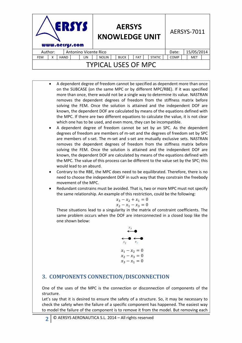
Redundant constrains must be avoided. That is, two or more MPC must not specify the same relationship. An example of this restriction, could be the following:

These situations lead to a singularity in the matrix of constraint coefficients. The same problem occurs when the DOF are interconnected in a closed loop like the one shown below:

3. COMPONENTS CONNECTION/DISCONNECTION One of the uses of the MPC is the connection or disconnection of components of the structure. Let’s say that it is desired to ensure the safety of a structure. So, it may be necessary to check the safety when the failure of a specific component has happened. The easiest way to model the failure of the component is to remove it from the model. But removing each


AERSYS-7011


TYPICAL USES OF MPC


component from the corresponding NASTRAN run would give as a result at least as many NASTRAN files as component failures exist. Therefore, in order to simplify the file management, MPC can be used. This kind of model consists of a main structure and the components that fail. The components are joined with the structure by means of MPC which allow the user to connect and disconnect them calling or not the MPC card in the case control SUBCASE. An example code of this kind of model is shown below:

SOL 101 CEND ... SUBCASE 1 SPC=1 ... SUBCASE 2 SPC=2 MPC=101 ... SUBCASE 3 SPC=3 MPC=102 ... BEGIN BULK $1111111222222223333333344444444555555556666666677777777 GRID 2 100. 5. 0.52 GRID 3 100. 5. 0.52 … MPC 1 3 1 1. 2 1 -1. MPC 1 3 2 1. 2 2 -1. MPC 1 3 3 1. 2 3 -1. MPC 1 3 4 1. 2 4 -1. MPC 1 3 5 1. 2 5 -1. MPC 1 3 6 1. 2 6 -1. ... MPCADD 101 1 5 6 MPCADD 105 5 9 11

In order to join the different MPC, a MPCADD card is used. The use of these cards is needed since most of the time there are more than one failing component. Each MPC


AERSYS-7011


TYPICAL USES OF MPC


normally joins each component with the main structure. Most of the times the MPCADD will contain all the MPC connecting each component except one, as the failure modes are usually defined as the failure of each component (and not the failure of several components together). This kind of MPC are composed by two nodes which are coincident (one of the main structure and one of the component) and whose DOF (all of them) are related with +1 and -1 coefficients. The analysis coordinate frame of both nodes should be the same. This, way it is ensured that:

TXnode3=TXnode2 TYnode3=TYnode2 TZnode3=TZnode2 RXnode3=RXnode2 RYnode3=RYnode2 RZnode3=RZnode2

Meaning, that node 2 (main structure) and node 3 (component) move together (the component is “bonded” to the main structure). It is similar to using an RBE2 between coincident nodes, but using MPC makes it selectable on each SUBCASE whereas the RBE2 is always included on the SUBCASE. The nodes must be coincident because otherwise spurious forces would be generated. An example of spurious forces is shown below:

Figure 1: Spurious forces example

For that structure, the single point constraints expected would be an axial force in the same direction than P and a moment. As a consequence of this, the OLOAD RESULTANT and the SPCFORCE RESULTANT are different. But the difference is taken into account by the MPCFORCE RESULTANT. This MPCFORCE takes or provides extra forces/moments that are not coming from the real structure. So as a consequence, the structure is not analysed properly.


AERSYS-7011


TYPICAL USES OF MPC


4. VIRTUAL DEFLECTION In some structures, there are parts which are moveable, such as the ailerons, the flaps or the rudder of an airplane. When the structure is analysed, there are different load cases in which the moveable components have different positions. So, it must be taken into account in the FEM of the structure. The “easiest” way to take into account the different deflections is to have as many models as needed with the components in their real position. For example, if the rudder positions for the load cases are ±30°, ±15° and 0°, it will be necessary to have 5 different models. This is not the best way to analyse the structure since there will be too many files. And additionally, each of the models will need a modification if there is an update of the properties, which involves a lot of time. So, the best way to solve this situation is the use of virtual deflection. The virtual deflection consists in a MPC which joins the moveable part with the rest of the structure. Thus, there will be only one model with the rudder at 0° (as a reference). Before explaining the MPC implementation, a sketch of the MPC is shown below for clarification.

Figure 2: FEM vs real structure for 0° configuration

51 42


AERSYS-7011


TYPICAL USES OF MPC


Figure 3: FEM vs real structure for θ° configuration

The FEM model is the same for all the possible rotation configurations, no translations of nodes is required to position the moveable component which remains always at 0º (as a reference). In the FEM model, the MPC relates the two nodes which are coincident: One of the main structure (node 42), and one of the moveable component (node 51). If there were only one configuration, the previous nodes would be the same, and the MPC would not be used. Let’s see an example in order to understand how it works: Let’s say that the moveable component has been deflected 15° and the moveable component loads in the hinge (shown on the moveable component axis system) are as the ones shown in the sketch below.

Figure 4: Forces in the moveable component

These forces will be transferred to the main structure by means of the hinge, giving as a result the forces plotted in the following figure (main structure axis system). As the node of the structure has a coordinate system different to the previous one, it is necessary to transform the previous forces to the structure coordinate system.

51 42


AERSYS-7011


TYPICAL USES OF MPC


Figure 5: Forces in the main structure

The transformation process that has been explained above is the transformation that the MPC must perform because the moveable component will not be physically rotated 15º on the FEM. It is easy to see that the relation between the forces must be the same than the relation between the displacements. So, after knowing the relation between the displacements it is possible to step up to the MPC relation. When the component is deflected, the nodes coordinate system would have the following configuration.

Figure 6: Nodes coordinate system for deflected configuration

Therefore the MPC equations would give the code which is displayed below:

MPC 100 51 1 0.5 51 2 -0.866 42 1 -1. MPC 100 51 1 0.866 51 2 0.5 42 2 -1. MPC 100 51 3 1. 42 3 -1.

Therefore, writing down the equation of the MPC:

The MPC equations simulate the transfer of loads from the moveable component to the main structure taking into account the deflection of the component. The relations are

cos(θ)

51 42

sin(θ)

-sin(θ)


AERSYS-7011


TYPICAL USES OF MPC


functions which depend on θ, therefore there must be a set of MPC for each component deflection. After having obtained the MPC for each deflection, it is possible to particularise them to the 0° deflection. In this configuration, the real structure and the FEM structure have the same configuration. Therefore MPC will represent a coincident node relation, that is, like the chapter above. The NASTRAN code for this configuration is shown below.

MPC 100 51 1 1. 42 1 -1. MPC 100 51 2 1. 42 2 -1. MPC 100 51 3 1. 42 3 -1.

Note that the reference coordinate systems of the nodes are as the one shown below.

Figure 7: Nodes coordinate system for non deflected configuration

Therefore, writing down the equations of the MPC:

As it can be seen in the previous code, the MPC 100 relates the DOF 1, 2 and 3 of the nodes 51 and 42. Only the displacements relations (no rotations) have been considered. That is because the nodes are placed in the hinge and therefore the rest of DOF do not have any influence. For other situations it could be possible to take into account more DOF which could be easily added with the idea explained on this chapter. One important topic of the virtual deflection is the interpretation of the displacements of the moveable component. Let’s say that after performing the NASTRAN run, the displacements of the component are obtained, and they are as the ones shown below:

Figure 8: Post-process displacements

51 42

51 42


AERSYS-7011


TYPICAL USES OF MPC


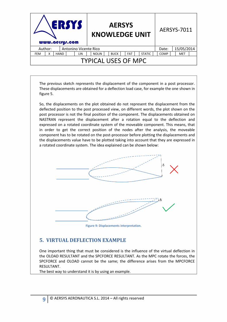
The previous sketch represents the displacement of the component in a post processor. These displacements are obtained for a deflection load case, for example the one shown in figure 5. So, the displacements on the plot obtained do not represent the displacement from the deflected position to the post processed view, on different words, the plot shown on the post processor is not the final position of the component. The displacements obtained on NASTRAN represent the displacement after a rotation equal to the deflection and expressed on a rotated coordinate system of the moveable component. This means, that in order to get the correct position of the nodes after the analysis, the moveable component has to be rotated on the post-processor before plotting the displacements and the displacements value have to be plotted taking into account that they are expressed in a rotated coordinate system. The idea explained can be shown below:

Figure 9: Displacements interpretation.

5. VIRTUAL DEFLECTION EXAMPLE One important thing that must be considered is the influence of the virtual deflection in the OLOAD RESULTANT and the SPCFORCE RESULTANT. As the MPC rotate the forces, the SPCFORCE and OLOAD cannot be the same; the difference arises from the MPCFORCE RESULTANT. The best way to understand it is by using an example.


AERSYS-7011


TYPICAL USES OF MPC


Figure 10: Real structure example

Figure 11: Virtual deflection structure

In the previous structure, there are two beams which are joined by means of MPC in the nodes 2 and 3. The beam 1-2 represents the main structure which is fixed by a clamp at node 1 and the beam 3-4 represents the moveable component which can be deflected an angle θ. The load is applied in the node 4 (moveable component), so the MPC would transform it properly. The structure has been analysed with two different configurations, θ = 0° and 45°. The forces for all the MPC configuration and the non deflected configuration are as follows:

Figure 12: Forces and moments for non-deflected configuration

0° configuration An extract of the NASTRAN code of the MPC case is shown below:

FORCE 1 4 0 100. 1. 1. 1. MOMENT 1 4 0 100. 1. 1. 1. ... MPC 1 2 1 1. 3 1 -1. MPC 1 2 2 1. 3 2 -1. MPC 1 2 3 1. 3 3 -1. MPC 1 2 4 1. 3 4 -1. MPC 1 2 5 1. 3 5 -1. MPC 1 2 6 1. 3 6 -1.


AERSYS-7011


TYPICAL USES OF MPC


The MPC relates directly the corresponding DOF. The structure is loaded with 100 units in each direction. In this case, the MPCFORCE RESULTANT is null, so the SPCFORCE RESULTANT and the OLOAD RESULTANT are coincident (with opposite sign). As the MPC do not deflects the moveable component, the displacements obtained are the same on both sides. That is, it is not necessary to transform the displacements obtained. As it can be seen in the NASTRAN code, all the DOF have been related. So, this represents a rigid joint in which all loads are transferred.

45° configuration Two options will be tested to see the difference: A rotation by using the MPC and a rotation by physically moving the node 4: By physically moving node 4 As the moveable component in the real structure is deflected. The NASTRAN code for the forces if the MPC were not used and the beam 3-4 was moved by translating node 4 with deflection of 45º would be as follows (note the coincidence with the SPCFORCES RESULTANS below, focus on the forces as the moments have additional components due to the offsets):

FORCE 1 4 0 100. 0. 1.4142 1. MOMENT 1 4 0 100. 0. 1.4142 1.

Figure 13: Forces in the real structure

For this configuration: OLOAD+SPCFORCE=0. The displacements for the configuration without the MPC (beam 3-4 physically rotated 45º and external loads properly adjusted) are:

Figure 14: Displacements without MPC


AERSYS-7011


TYPICAL USES OF MPC


By using the MPC The extract of the NASTRAN code of the MPC case is shown below:

FORCE 1 4 0 100. 1. 1. 1. MOMENT 1 4 0 100. 1. 1. 1. ... MPC 1 3 1 0.7071 3 2 -0.7071 2 1 -1. MPC 1 3 2 0.7071 3 1 0.7071 2 2 -1. MPC 1 2 3 1. 3 3 -1. MPC 1 3 4 0.7071 3 5 -0.7071 2 4 -1. MPC 1 3 5 0.7071 3 4 0.7071 2 5 -1. MPC 1 2 6 1. 3 6 -1.

In this case, the MPC relates the DOF to satisfy the relations shown in the previous chapters. For this configuration, as the MPC deflects the moveable component, the MPCFORCE RESULTANT is not null. Therefore, OLOAD+SPCFORCE≠0. In this case, the difference between the OLOAD and the SPCFORCE are created by the MPC. So the MPCFORCE takes into account this difference, giving as a result that OLOAD+SPCFORCE+MPCFORCE=0.


AERSYS-7011


TYPICAL USES OF MPC


Figure 15: OLOAD; SPCFORCE and MPCFORCE for the MPC configuration

As explained above, the displacements have to be interpreted in the correct way.

Figure 16: Displacements with MPC

As it can be seen, for nodes 1 and 2 (main structure) the displacements are the same for both configurations. The displacements of the moveable component (node 4) in the case with MPC are referenced to a different coordinate system. To see it easier, a sketch is displayed below:

Figure 17: Real structure (above) and MPC structure (below)

As it can be seen in the previous sketch, the reference coordinate system for the virtual deflection is not the same as the one used in the real structure. The coordinate system of the MPC is rotated (θ=45°). So, in order to compare the displacements of both configurations, it is necessary to rotate them. The equations of the rotation are plotted below:

Grid

reference

coordinate

system

T1

T2


AERSYS-7011


TYPICAL USES OF MPC


In this case (θ=45°), for the node 4.

It is important to remember that the displacements obtained must be considered as they were also deflected. That is, the displacement for the MPC case will be as follows.

Figure 18: Displacements of the MPC structure

In the previous sketch, the black solid line represents the structure which is introduced in NASTRAN (input of the NASTRAN run) and the blue solid line is the fake final position with the displacements obtained on the NASTRAN run. This is what a post-processor would represent. The dotted black lines represent the real position of the moveable component and the dotted blue line is the real final position with the displacements obtained on the NASTRAN run. This is the correct interpretation of the NASTRAN results.

aersys aersys-7011 knowledge unit · knowledge unit aersys-7011 author: ... but using mpc makes it...

Documents